Download - BUAD306

BUAD306
Chapter 3 – Forecasting

Everyday Forecasting
Weather Time Traffic Other examples???

Forecasting
What is forecasting? How is it used in business? Approaches to forecasting Forecasting techniques

What is Forecasting?
Forecast: A statement about the future
Used to help managers:Plan the systemPlan the use of the system

Use of Forecasts
Accounting Cost/profit estimates
Finance Cash flow and funding
Human Resources Hiring/recruiting/training
Marketing Pricing, promotion, strategy
MIS IT/IS systems, services
Operations Schedules, MRP, workloads
Product/service design New products and services

Forecasting Basics
Assumes causal system past ==> future
Forecasts rarely perfect because of randomness
Forecasts more accurate for groups vs. individuals
Forecast accuracy decreases as time horizon increases
Elements of a Good Forecast
Timely – feasible horizon Reliable – works consistently Accurate – degree should be stated Expressed in meaningful units Written – for consistency of usage Easy to Use - KISS

Approaches to Forecasting
Judgmental – subjective inputs Time Series – historical data Associative – explanatory variables

Judgmental Forecasts
Executive Opinions Accuracy?? Sales Force Feedback Bias??? Consumer Surveys Outside Opinions Industry experts

What would you rather evaluate?
Period A B C
1 30 18 46
2 34 17 26
3 32 19 27
4 34 19 23
5 35 22 22
6 30 23 48
7 34 23 29
8 36 25 20
9 29 24 14
10 31 26 18
11 35 27 47
12 31 28 26
13 37 29 27
14 34 31 24
15 33 33 22
16
0
10
20
30
40
50
60
1 2 3 4 5 6 7 8 9 10 11 12 13 14 15

Time Series Forecasts
Based on observations over a period of time
Identifies:Trend – LT movement in dataSeasonality – ST variationsCycles – wavelike variationsIrregular Variations – unusual eventsRandom Variations – chance/residual
Examples on the board

Forecast Variations
Trend
Irregularvariation
Seasonal Variations
908988
Cycles

Naïve Forecasting
Simple to use Minimal to no cost Data analysis is almost nonexistent Easily understandable Cannot provide high accuracy Can be a standard for accuracy
Examples on the board & HW#1…

HW Problem 1Day Muffins Buns Cupcakes
1 30 18 46
2 34 17 26
3 32 19 27
4 34 19 23
5 35 22 22
6 30 23 48
7 34 23 29
8 36 25 20
9 29 24 14
10 31 26 18
11 35 27 47
12 31 28 26
13 37 29 27
14 34 31 24
15 33 33 22
16

HW Problem 1
0
10
20
30
40
50
60
1 2 3 4 5 6 7 8 9 10 11 12 13 14 15
MuffinsBunsCupcakes

Techniques for Averaging
Moving average Weighted moving average Exponential smoothing

Simple Moving Average
MAn = n
Aii = 1n
Where: i = index that corresponds to periods n = number of periods (data points) Ai = Actual value in time period I MA = Moving Average Ft = Forecast for period t

Period Sales
1 3520
2 2860
3 4005
4 3740
5 4310
6 5001
7 4890
8 ??
Four period moving average for period 7:
Four period moving average for period 8:
Four period moving average for period 9 if actual for 8 = 5025:
Example 1: Moving Average

Weighted Moving Average
Similar to a moving average, but assigns more weight to the most recent observations.
Total of weights must equal 1.
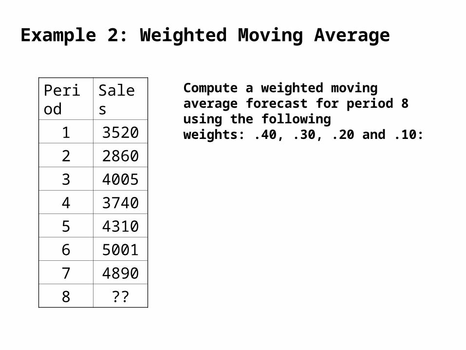
Compute a weighted moving average forecast for period 8 using the following weights: .40, .30, .20 and .10:
Example 2: Weighted Moving Average
Period Sales
1 3520
2 2860
3 4005
4 3740
5 4310
6 5001
7 4890
8 ??
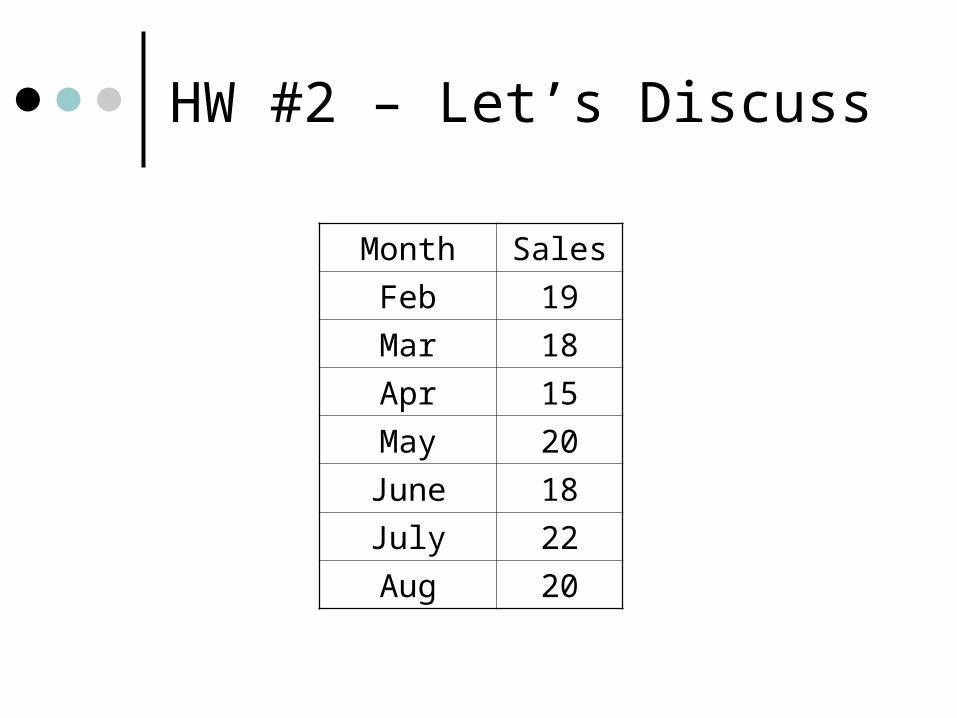
HW #2 – Let’s Discuss
Month Sales
Feb 19
Mar 18
Apr 15
May 20
June 18
July 22
Aug 20

Calculating Error
Mathematically:
et = At - Ft
Let’s discuss examples on board…

Exponential Smoothing
Premise--The most recent observations might have the highest predictive value….
Therefore, we should give more weight to the more recent time periods when forecasting.

Exponential Smoothing
Ft = Ft-1 + (At-1 - Ft-1)
Next forecast = Previous forecast + (Actual -Previous Forecast)
Smoothing Constant

About
= Smoothing constant selected by forecaster
It is a percentage of the forecast error The closer the value is to zero, the
slower the forecast will be to adjust to forecast errors (greater smoothing)
The higher the value is to 1.00, the greater the responsiveness to errors and the less smoothing
READ TEXT

Ft = Ft-1 + (At-1 - Ft-1)
Example 3: Exponential Smoothing
Assume a starting forecast of 4030 for period 3.
Given data at left and = .10, what would the forecast be for period 8?
Period Sales
1 3520
2 2860
3 4005
4 3740
5 4310
6 5001
7 4890
8 ??

Example 3: Exponential Smoothing
Period Act Forecast Calc Fore
3 4005 4030
4 3740
5 4310
6 5001
7 4890
8

HW #2 – Let’s Discuss
Month Sales
Feb 19
Mar 18
Apr 15
May 20
June 18
July 22
Aug 20

Techniques for Seasonality
Seasonal Variations – regularly repeating movements in series values that can be tied to recurring events
Computing Seasonal Relatives: READ THE TEXTLook at HW #12 – don’t have to know this for exam

Using Seasonal Relatives
Allows you to incorporate seasonality or deseasonalize dataIncorporate: Useful when trend and
seasonality are apparentDeseasonalize – Remove seasonal
components to get a clearer picture of non-seasonal components

Example 4: Using Seasonal Relatives
A publisher wants to predict quarterly demand for a certain book for periods 9 and 16, which happen to be in the 3rd and 2nd quarters of a particular year. The data series consists of both trend and seasonality. The trend portion of demand is projected using the equation: yt=12,500 + 150.5t.
Quarter relatives are Q1= 1.3, Q2=.8, Q3=1.4, Q4=.9
Use this information to predict demand for periods 9 and 16.The trend values:
Applying the relatives:

HW #11 – Let’s Discuss
The following equation summarizes the trend portion of quarterly sales of condos over a long cycle. Prepare a forecast for each Q of 2014 and 1Q15.
Ft = 40 – 6.5t + 2t2
Ft = unit salest= 0 at 1Q 2012
Quarter Relative
1 1.1
2 1
3 .6
4 1.3

Assoc. Forecasting Technique:Simple Linear Regression
Predictor variables - used to predict values of variable interest
Regression - technique for fitting a line to a set of points
Least squares line - minimizes sum of squared deviations around the line

Linear Regression Assumptions
Variations around line are randomNo patterns are apparent
Deviations around the line should be normally distributed
Predictions are being made only in the range of observed values
Should use minimum of 20 observations for best results

Suppose you analyze the following data...
0
10
20
30
40
50
0 5 10 15 20 25
X Y7 152 106 134 15
14 2515 2716 2412 2014 2720 4415 347 17

The regression line has the following equation:
y c = a + bx
Where: y c = Predicted (dependent) variablex = Predictor (independent) variableb = slope of the linea = Value of y c when x=0
b = n (xy) - (x)(y)n(x2) - (x)2
a = y - bx n

Example 5 - Linear Regression:
Suppose that a manufacturing company made batches of a certain product. The accountant for the company wished to determine the cost of a batch of product given the following data:
Size of batch203040507080
100120150
Cost of batch (in 1000s)$1.43.44.13.86.76.67.8
10.411.7
Question… which is the dependent (y) and which is the independent (x) variable?
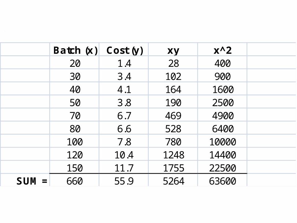
Batch (x) Cost (y) xy x^220 1.4 28 40030 3.4 102 90040 4.1 164 160050 3.8 190 250070 6.7 469 490080 6.6 528 6400
100 7.8 780 10000120 10.4 1248 14400150 11.7 1755 22500
SUM = 660 55.9 5264 63600

We are now ready to determine the values of b and a:
b = n (xy) - (x)(y) = 9 (5264) - (660)(55.9)
n(x2) - (x)2 9(63600) - (660)2
= 47376-36894 = 10482 =
572400-435600 136800
Batch (x) Cost (y) xy x^2SUM = 660 55.9 5264 63600
a = y - bx = 55.9 - .0766(660) = n 9

Our linear regression equation:
y c = a + bx
y c =
What is the cost of a batch of 125 pieces?
y c =

Batch (x) Cost (y)20 1.430 3.440 4.150 3.870 6.780 6.6
100 7.8120 10.4150 11.7 0
24
6
8
1012
14
0 100 200Batch size
Co
st
Series1
Linear (Series1)

Problem #7
Freight car
loadings at a
busy port are as
follows:
Week # Week #
1 220 10 380
2 245 11 420
3 280 12 450
4 275 13 460
5 300 14 475
6 310 15 500
7 350 16 510
8 360 17 525
9 400 18 541

Problem #7Period (t) Loads (y) t^2 t * y
1 220 1 220 2 245 4 490 3 280 9 840 4 275 16 1,100 5 300 25 1,500 6 310 36 1,860 7 350 49 2,450 8 360 64 2,880 9 400 81 3,600
10 380 100 3,800 11 420 121 4,620 12 450 144 5,400 13 460 169 5,980 14 475 196 6,650 15 500 225 7,500 16 510 256 8,160 17 525 289 8,925 18 541 324 9,738
SUM 171 7,001 2,109 75,713
b = n (xy) - (x)(y)
n(x2) - (x)2
a = y - bx n

Correlation (r)
A measure of the relationship between two variables
• Strength• Direction (positive or negative)
Ranges from -1.00 to +1.00• Correlation close to 0 signifies a weak
relationship – other variables may be at play
• Correlation close to +1 or -1 signifies a strong relationship

Calculating a Correlation Coefficient
r = n( xy) - ( x)( y)
n( x2)- ( x)2 * n( y2) - ( y)2

Batch (x) Cost (y) xy x^2 y^2SUM = 660 55.9 5264 63600 439.11
r = n( xy) - ( x)( y)
n( x2)- ( x)2 * n( y2) - ( y)2
r = 9 () - ()()9()- ()2 * 9() - ()2
r = 47376 - 36894 = 10482 = .985 136800 * 827.18 369.86 * 28.76
Example 6: Continued

Coefficient of Determination (r2)
How well a regression line “fits” the data
Ranges from 0.00 to 1.00 The closer to 1.0, the better the fit

0
5
10
15
0 50 100 150 200
Batch size
Co
st
Series1
Linear(Series1)
r = .985r2 = .9852 = .97
Example 6: Continued
Conclusion of Example
R = .985 Positive, close to one
R2 = .9852 = .97Closer to one, the better the fit to the
line

Forecast Accuracy
Error - difference between actual value and predicted value
Mean absolute deviation (MAD)Average absolute error
Mean squared error (MSE)Average of squared error
Why can’t we simply calculate error for each observed period and then select the technique with the lowest error?

Error Example
Period Actual 3PMA 5PMA3P WMA.6, .3, .1 EX SM .2 LR
1 55 55.692 60 55 60.663 75 56 65.634 58 63.33333 68.5 59.8 70.65 80 64.33333 63.3 59.44 75.576 90 71 65.6 72.9 63.552 80.547 70 76 72.6 83.8 68.8416 85.518 92 80 74.6 77 69.07328 90.489 100 84 78 85.2 73.65862 95.45
10 87.33333 86.4 94.6 78.9269 100.42
#errors? 6 4 6 8 9
Does the # of errors calculated impact the "accuracy" comparison???

Calculating Error
Mathematically:
What do the negative errors mean?
How do they affect total error?
et = At - Ft

Calculating MAD and MSE
MAD = Actual forecastn
MSE = Actual forecast)
-1
2n
(

Conclusions with MAD & MSE
The MAD and MSE can be used as a comparison tool for several forecasting techniques.
The forecasting technique that yields the lowest MAD and MSE is the preferred forecasting method.

MAD & MSE Comparison
Tech MAD MSE
3 Period MA 3.6 8.1
Exp Sm .02 2.2 5.6
Exp Sm .04 2.6 6.1
Which technique would you select for your forecast approach?


