BUAD306

Chapter 19 – Linear Programming

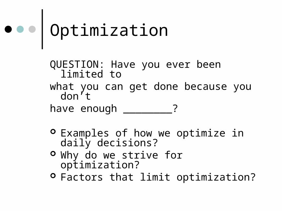
Optimization

QUESTION: Have you ever been limited towhat you can get done because you don’thave enough ________?

Examples of how we optimize in daily decisions?

Why do we strive for optimization? Factors that limit optimization?

What is Linear Programming

A model consisting of linear relationships that represent a firm’s objective and resource constraints

Problems are typically referred to as constrained optimization problems

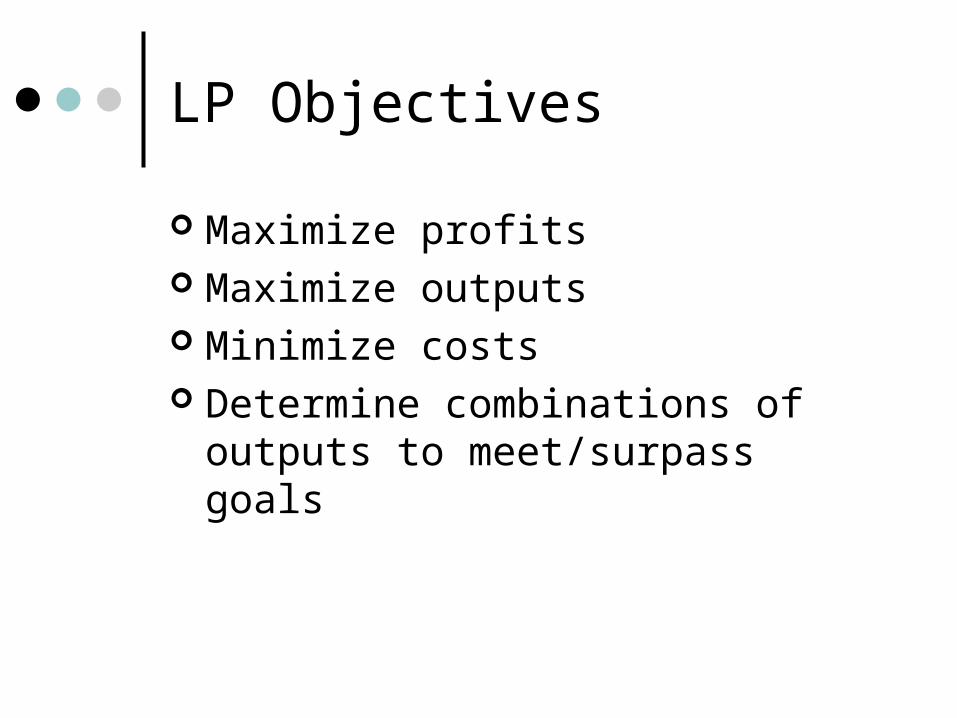
LP Objectives

Maximize profits Maximize outputs Minimize costs Determine combinations of outputs to

meet/surpass goals

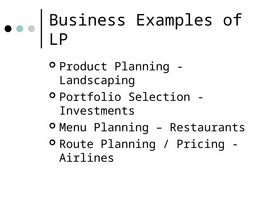
Business Examples of LP

Product Planning - Landscaping Portfolio Selection - Investments Menu Planning – Restaurants Route Planning / Pricing - Airlines

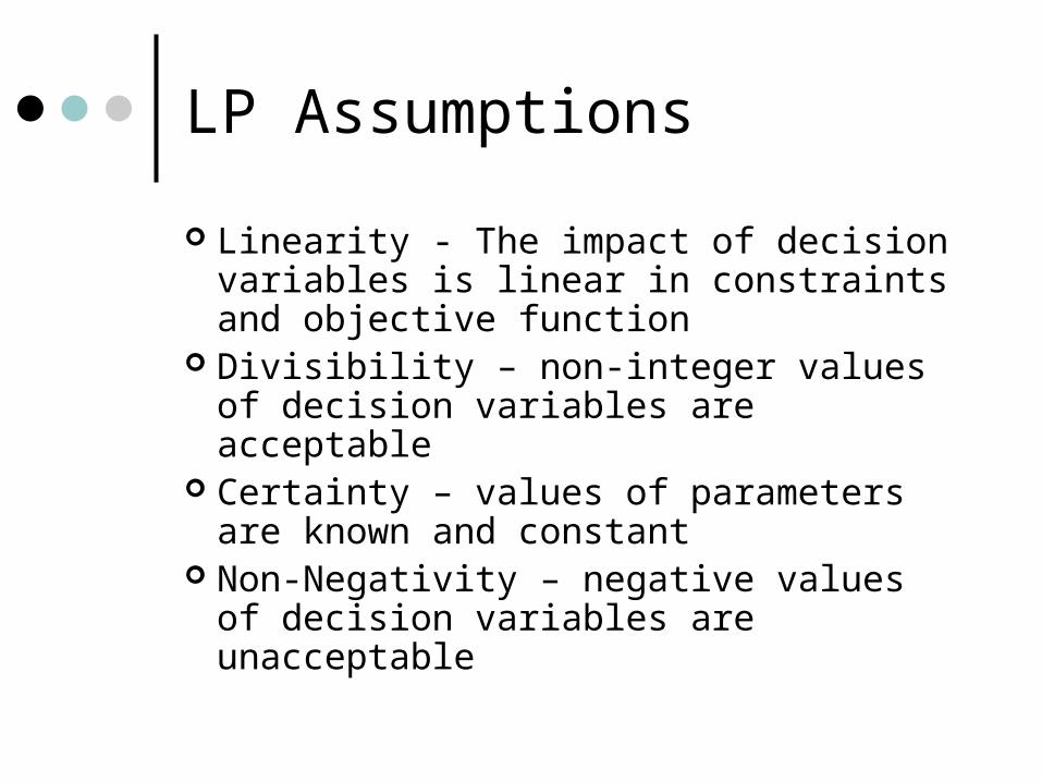
LP Assumptions

Linearity - The impact of decision variables is linear in constraints and objective function

Divisibility – non-integer values of decision variables are acceptable

Certainty – values of parameters are known and constant

Non-Negativity – negative values of decision variables are unacceptable

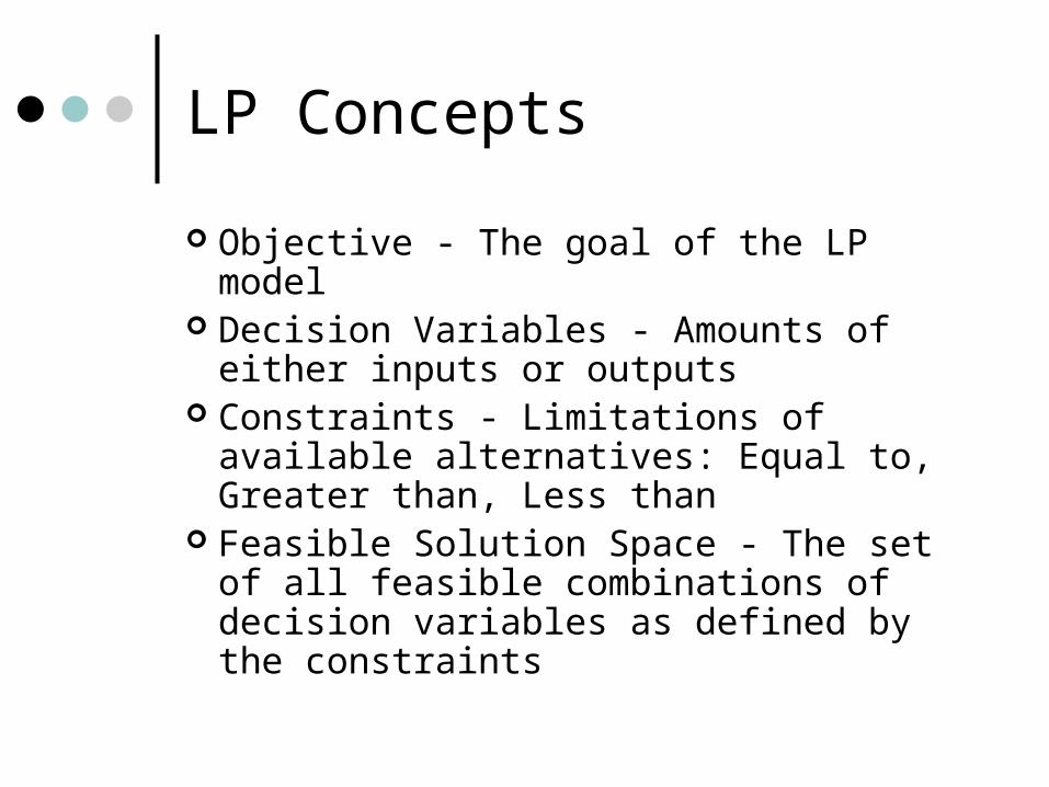
LP Concepts

Objective - The goal of the LP model Decision Variables - Amounts of either

inputs or outputs Constraints - Limitations of available

alternatives: Equal to, Greater than, Less than

Feasible Solution Space - The set of all feasible combinations of decision variables as defined by the constraints

Constraints

Restrictions on the company’s resourcesTimeLaborEnergyMaterialsMoney

Restriction guidelines recipe for making food productsengineering specifications

LP Steps

Step 1: Set up LP model

Step 2: Plot the constraints

Step 3: Identify the feasible solution

space

Step 4: Plot the objective function

Step 5: Determine the optimal solution

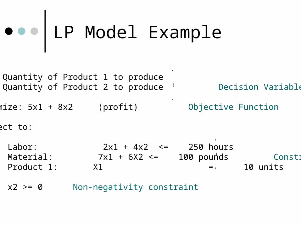
LP Model Example

X1 = Quantity of Product 1 to produceX2 = Quantity of Product 2 to produce Decision Variables

Maximize: 5x1 + 8x2 (profit) Objective Function

Subject to:

Labor: 2x1 + 4x2 <= 250 hoursMaterial: 7x1 + 6X2 <= 100 pounds ConstraintsProduct 1: X1 = 10 units

x2 >= 0 Non-negativity constraint

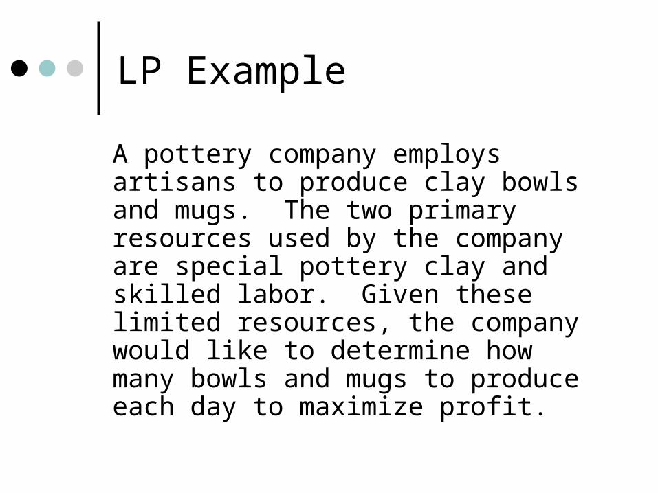
LP Example

A pottery company employs artisans to produce clay bowls and mugs. The two primary resources used by the company are special pottery clay and skilled labor. Given these limited resources, the company would like to determine how many bowls and mugs to produce each day to maximize profit.

The two products have the following resource requirements for production and selling price per item produced:

ProductLabor

(h/unit)Clay

(lb/unit)Revenue($/unit)

Bowl 1 3 20Mug 2 2 20

There are 40 hours of labor and 60 pounds of clay available each day.

Formulate this problem as an LP model.

Decision variables: x1 = # of bowls to produce

x2 = # of mugs to produce

There are 40 hours of labor and 60 pounds of clay available each day. What are the decision variables, objective function & constraints?

Objective: Maximize Z = 20x1 + 20x2

Constraints: Labor: x1 + 2x2 <= 40

Clay: 3x1 + 2x2 <= 60

Non- Neg: x1, x2 >=0

ProductLabor

(h/unit)Clay

(lb/unit)Revenue($/unit)

Bowl 1 3 20Mug 2 2 20

Plot Constraints

Step 1: For each constraint, set x1 = 0, get value for x2

Step 2: For each constraint, set x2 = 0, get value for x1

Step 3: Plot these as coordinates and then draw constraint lines

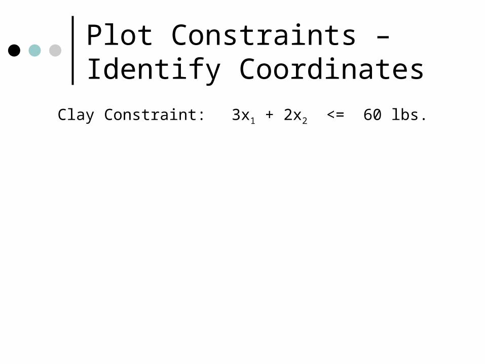
Plot Constraints – Identify Coordinates

Labor Constraint: x1 + 2x2 <= 40 hrs

Plot Constraints – Identify Coordinates

Clay Constraint: 3x1 + 2x2 <= 60 lbs.

Plot Constraints

0

5

10

15

20

25

30

35

40

45

0 10 20 30 40 50

x1

x2

50

Clay

Labor

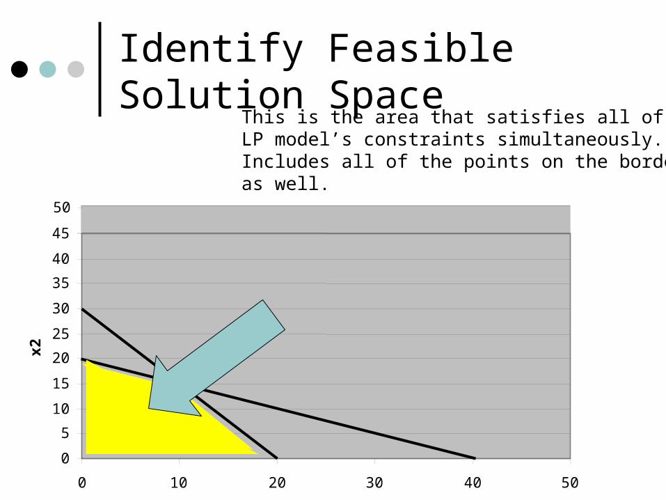
Identify Feasible Solution Space

This is the area that satisfies all of the LP model’s constraints simultaneously. Includes all of the points on the borders as well.

0

5

10

15

20

25

30

35

40

45

0 10 20 30 40 50

x2

50

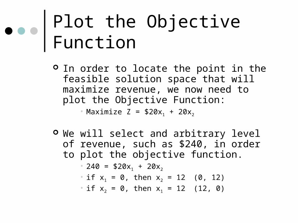
Plot the Objective Function

In order to locate the point in the feasible solution space that will maximize revenue, we now need to plot the Objective Function:

• Maximize Z = $20x1 + 20x2

We will select and arbitrary level of revenue, such as $240, in order to plot the objective function.

• 240 = $20x1 + 20x2

• if x1 = 0, then x2 = 12 (0, 12)• if x2 = 0, then x1 = 12 (12, 0)

Identify Feasible Solution Space Observation: Every point on this

Line in the feasible solution areaWill result in a revenue of $240.(Every combination of X1 and X2on this line in this space will yield an $240 revenue total.)

0

5

10

15

20

25

30

35

40

45

0 10 20 30 40 50

x2

50

Identify Feasible Solution Space

0

5

10

15

20

25

30

35

40

45

0 10 20 30 40 50

x2

50

Shift the objective function line to locate the optimal solution point.

Finding the Optimal Solution

As you increase the revenue from $240, the line will move up and to the right in a parallel manner.

The point where it moves thru the boundary of the feasible space contains the points farthest from the origin– which correspond to the points yielding the greatest revenue.

Note: Once it passes outside the feasible solution area, it’s no longer a feasible revenue line because of constraint limitations.

Finding the Optimal Solution

As we shift the objective function line away from the origin, we search for the farthest point that is still in/on the feasible solution.

As been proven mathematically, the solution point will not only be on the boundary of the feasible solution space, it will be at one of the corners of the boundary where two constraints intersect– the most you can use of those constraints. This is called an extreme point.

Solving for the Optimal Solution

Given our constraint equations:• x1 + 2x2 = 40 (Labor)• 3x1 + 2x2 = 60 (Clay)

We set them equal to each other and solve for the optimal quantities of X1 and X2:

Solving for the Optimal Solution

Thus, the optimal solution is to produce ___ bowls and ____ mugs for a maximized revenue of $___________.

Objective Function: Maximize: 20x1 + 20x2

Z =

Confirm Answer

0

5

10

15

20

25

30

35

40

45

0 10 20 30 40 50

x1

x2

50

(0,0) =

(0,20) =

(20,0) =

(10,15) =

Delstate Jewelers manufacturers two types of semi-precious gems for sale to its wholesale customers, Gem 1 and Gem 2. Delstate realizes revenue of $4.00 for each Gem 1 sold and revenue of $3 per gem for each Gem 2 sold. To produce the gems, the company must cut and polish each gem. The company is limited to a certain number of minutes for each machine that is used in the cutting and polishing process as shown in the table below. Given this information, determine the optimal quantities of Gem 1 and Gem 2 that maximize revenue.

   

Product Cutting Polishing

Gem 1 14 7

Gem 2 6 12

Total Minutes Available 84 84

Example #1

Slack and Surplus

A slack variable is a variable representing unused resources added to a <= constraint to make it an equality.

A surplus variable is a variable representing an excess above a resource requirement that is subtracted from a >= constraint to make it an equality.

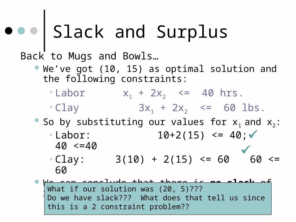
Slack and SurplusBack to Mugs and Bowls…

We’ve got (10, 15) as optimal solution and the following constraints:

• Labor x1 + 2x2 <= 40 hrs.• Clay 3x1 + 2x2 <= 60 lbs.

So by substituting our values for x1 and x2:

• Labor: 10+2(15) <= 40; 40 <=40• Clay: 3(10) + 2(15) <= 60 60 <= 60

We can conclude that there is no slack of resources given our optimal solution

What if our solution was (20, 5)??? Do we have slack??? What does that tell us since this is a 2 constraint problem??

Example #2

A leather shop makes custom, hand-tooled briefcases and luggage. The shop makes a $400 profit from each briefcase and $200 profit from each piece of luggage. The shop has a contract to provide a local store with exactly 30 items each month. A tannery supplies the shop with at least 80 square yards of leather per month. The shop must at least use this amount, but can use more if needed. Each briefcase requires 2 square yards of leather, each piece of luggage requires 8 square yards of leather. From past performance, the shop owner knows that they cannot make more than 20 briefcases per month.

Determine the number of briefcases and luggage to produce each month in order to maximize revenue. Formulate an LP model and solve graphically. Determine the optimal quantities of briefcases and luggage and the maximized revenue amount. Also determine if there is any slack or surplus.

In Class Example

max 5x1 + 6x2

stA 2x1+3x2<=60B 4x1+x2<=80C x1+x2<=50N/N x1, x2 >=0

Add’l LP Considerations

Binding Constraints Redundant Constraints Multiple Optimal Solutions Slack & Surplus

Binding Constraint

When a constraint forms the optimal corner point of the feasible solution space, it is BINDING.

Redundant Constraint

A constraint that does not form a unique boundary of the feasible solution space.

Its removal would not alter the feasible solution space.

Multiple Optimal Solutions

In some instances, you may get an objective function which is parallel to a constraint line

This ends up NOT being tangent to the feasible solution space!

Sensitivity Analysis

Assessing the impact of potential changes to the numerical values of an LP model

• Objective function coefficients

• Right-hand values of constraints

• Constraint coefficients

Max 20x1 + 20x2

S.T.

L: 1x1 + 2x2 <= 40C: 3x1 + 2x2 <= 60

N/N: x1, x2 >=0

LINDO

Computer-based modeling system for solving linear programming problems

All PCs in the Purnell computer lab have LINDO installed

LINDO Steps

Designate functions within LINDOMax/MinConstraints

Solve with Sensitivity Analysis

LINDO AnswersNotice that the resultsprovide the same answerswe obtained in our graphicalapproach.

Objective Function RangesWith this report, we can determine the range in which the objective coefficients can exist before the optimal solution changes:

Revenue coefficient for Bowls can range between 10 and 30 without impacting solution

Revenue coefficient for Mugs can range between 20 and 60 without impacting solution

RHS Ranges With this report, we can determine the range in which the RHS of the constraints can change while yielding the same savings/cost indicated by the Shadow (Dual) Price

RHS for Labor constraint can range between 33.33 and 100

RHS for Clay constraint can range between 20 and 60

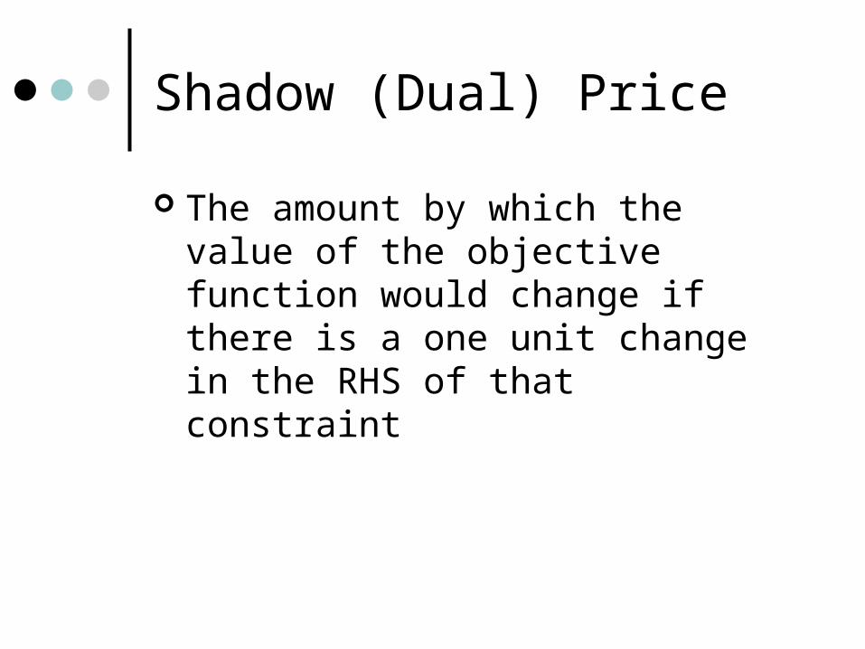
Shadow (Dual) Price

The amount by which the value of the objective function would change if there is a one unit change in the RHS of that constraint

Shadow (Dual) Pricing

If constraint has slack, shadow price = 0 Increasing or decreasing RHS has no

effect - would only increase slack/surplus If constraint is binding, shadow price =

the amount objective function will change for each one unit change in the RHS

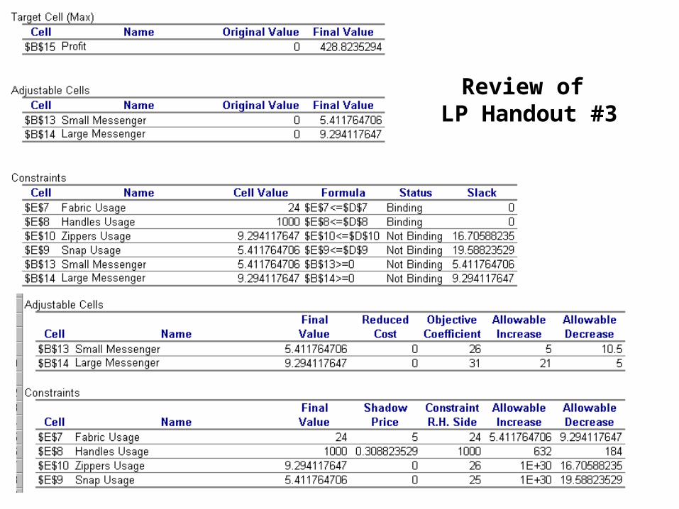
Review of LP Handout #3

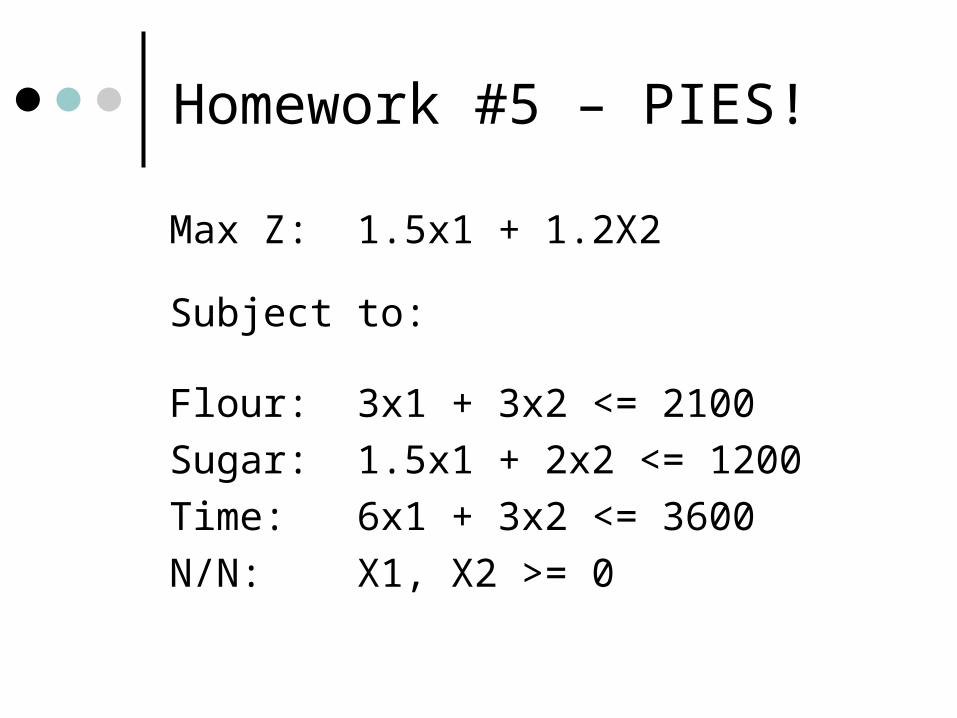
Homework #5 – PIES!

Max Z: 1.5x1 + 1.2X2

Subject to:

Flour: 3x1 + 3x2 <= 2100

Sugar: 1.5x1 + 2x2 <= 1200

Time: 6x1 + 3x2 <= 3600

N/N: X1, X2 >= 0

Homework #5