
Bank Lending and Property Prices: Some International Evidence*
Boris Hofmann
Zentrum für Europäische Integrationsforschung University of Bonn
ABSTRACT
This paper analyses the patterns of dynamic interaction between bank lending and property prices based on a sample of 20 countries using both time series and panel data techniques. Long-run causality appears to go from property prices to bank lending. This finding suggests that property price cycles, reflecting changing beliefs about future economic prospects, drive credit cycles, rather than excessive bank lending being the cause of property price bubbles. There is also evidence of short-run causality going in both directions, implying that a mutually re-enforcing element in past boom bust cycles in credit and property markets cannot be ruled out.
*This paper was written while the author was a Visiting Research Fellow at the Hong Kong Institute for Monetary Research at the Hong Kong Monetary Authority. I am grateful to Stefan Gerlach, Olan Henry, Charles Goodhart, Jürgen von Hagen and seminar participants at the Hong Kong Monetary Authority for helpful comments and Steve Arthur for his help with the data. All remaining errors are my own responsibility.

2
1. Introduction
Over the last couple of years, the coincidence of cycles in credit and property markets has
been widely documented and discussed in the policy oriented literature (IMF, 2000, BIS,
2001). However, the question of the direction of causality between bank lending and property
prices has remained a rather unexplored issue. From a theoretical point of view, causality may
go in both directions. Property prices may affect bank lending via various wealth effects.
First, due to financial market imperfections, households and firms may be borrowing
constrained. As a result, households and firms can only borrow when they offer collateral, so
that their borrowing capacity is a function of their collateralisable net worth1. Since property
is commonly used as collateral, property prices are therefore an important determinant of the
private sector’s borrowing capacity. Second, a change in property prices may have a
significant effect on consumers’ perceived lifetime wealth2, inducing them to change their
spending and borrowing plans and thus their credit demand in order to smooth consumption
over the life cycle3. Finally, property prices affect the value of bank capital, both directly to
the extent that banks own assets, and indirectly by affecting the value of loans secured by
property4. Property prices therefore influence the risk taking capacity of banks and thus their
willingness to extend loans.
On the other hand, bank lending may affect property prices via various liquidity effects. The
price of property can be seen as an asset price, which is determined by the discounted future
stream of property returns. An increase in the availability of credit may lower interest rates
and stimulate current and future expected economic activity. As a result, property prices may
rise because of higher expected returns on property and a lower discount factor. Property can
also be seen as a durable good in temporarily fixed supply. An increase in the availability of
credit may increase the demand for housing if households are borrowing constrained. With
1 Basic references of this literature are Bernanke and Gertler (1989) and Kiyotaki and Moore (1997). For a survey see Bernanke, Gertler and Gilchrist (1998). An early reference is Fisher (1933). 2Data on the composition of household wealth, reported in OECD (2000), show that households hold a large share of their wealth in property. 3 The lifecycle model of household consumption was originally developed by Ando and Modigliani (1963). A formal exposition of the lifecycle model can be found in Deaton (1992) and Muellbauer (1994).
3
supply temporarily fixed because of the time it takes to construct new housing units, this
increase in demand will be reflected in higher property prices.
This potential two-way causality between bank lending and property prices may give rise to
mutually reinforcing cycles in credit and property markets5. A rise in property prices, caused
by more optimistic expectations about future economic prospects, raises the borrowing
capacity of firms and households by increasing the value of collateral. Part of the additional
available credit may also be used to purchase property, pushing up property prices even
further, so that a self-reinforcing process may evolve.
Little empirical research has been done on the relationship between credit and asset prices.
Most studies rely on a single equation set up, focusing either on bank lending or property
prices. Goodhart (1995) finds that property prices significantly affect credit growth in the UK
but not in the US. Hilbers, Lei and Zacho (2001) find that the change in residential property
prices significantly enters multivariate probit-logit models of financial crisis in industrialised
and developing countries. Borio and Lowe (2002) show that a measure of the aggregate asset
price6 gap, measured as the deviation of aggregate asset prices from their long-run trend,
combined with a similarly defined credit gap measure, is a useful indicator of financial
distress in industrialised countries.
Borio, Kennedy and Prowse (1994) investigate the relationship between credit to GDP ratios
and aggregate asset prices for a large sample of industrialised countries over the period 1970-
1992 using annual data. They focus on the determinants of aggregate asset price fluctuations,
hypothesising that the development of credit conditions as measured by the credit to GDP
ratio can help to explain the evolution of aggregate asset prices. They find that adding the
credit to GDP ratio to an asset pricing equation helps to improve the fit of this equation in
4 Chen (2001) develops an extension of the Kiyotaki and Moore (1997) model where an additional amplification of business cycles results from the effect of asset price movements on banks‘ balance sheets. An early reference for this argument is Keynes (1931). 5 The possibility of mutually re-enforcing cycles in credit and asset markets has already been stressed by Kindleberger (1978) and Minsky (1982). 6 Aggregate asset price indices are calculated as a weighted average of residential property prices, commercial property prices and equity prices. The weights are based on the share of each asset in national balance-sheets, which are derived based on national flow-of-funds data or UN standardised national accounts. The index weight of both residential and commercial property prices is on average above 80% so that property price movements dominate the movements of the aggregate asset price index.

4
most countries. Based on simulations they demonstrate that the boom-bust cycle in asset
markets of the late 1980s - early 1990s would have been much less pronounced or would not
have occurred at all had credit ratios remained constant. For a panel of four East Asian
countries (Hong Kong, Korea, Singapore and Thailand), Collyns and Senhadji (2001) find
that credit growth has a significant contemporaneous effect on residential property prices.
Based on this finding, they conclude that bank lending has contributed significantly to the real
estate bubble in Asia prior to the 1997 East Asian crisis.
All these studies potentially suffer from simultaneity problems because the potential two-way
relationship between credit and property prices is not controlled for. In two recent studies,
Hofmann (2001) and Gerlach and Peng (2002) analyse the relationship between bank lending
and property prices based on a multivariate empirical framework. Hofmann (2001) finds for a
set of 16 industrialised countries that including property prices in the empirical model is
imperative for the explanation of the long-run development of bank lending and that long-run
causality goes from property prices and real activity to bank lending. Based on impulse
response analysis Hofmann (2001) finds that property price innovations have a significantly
positive effect on bank lending and vice versa, suggesting a two-way relationship between
credit and property prices. The problem with this paper’s analysis is that the identified
patterns of causality are likely not to be invariant to the indentifying assumptions imposed
upon the estimated VARs. Gerlach and Peng (2002) overcome this problem by analysing the
direction of causality between bank lending and property prices in Hong Kong based on
standard regression techniques, controlling for potential simultaneity problems. They find that
long-run and short-run causality goes from property prices to lending, rather than conversely.
In the following I assess, based on time series and panel data techniques, the patterns of
dynamic interaction between bank lending and property prices for a sample of 20 countries
since the mid 1980s. The plan of the paper is as follows. The following Section 2 describes
the data. Section 3 tests and estimates long-run relationships between bank lending,
economic activity and property prices. In Section 4 I estimate error-correction models and
test for the patterns of long-run and short-run causality between bank lending and property
prices. Section 5 concludes.
5
2. Data
In the following sections I analyse the relationship between real aggregate bank lending, real
GDP as a measure of aggregate economic activity, real residential property prices and real
money market interest rates in 20 countries: the US, Japan, Germany, France, Italy, the UK,
Canada, Switzerland, Sweden, Norway, Finland, Denmark, Spain, the Netherlands, Belgium,
Ireland, Australia, New Zealand, Hong Kong and Singapore. The data for the industrialised
countries were taken from the IMF and the BIS database. Data for Hong Kong and Singapore
are from the CEIC database. Except for the nominal interest rate, all data were seasonally
adjusted using the Census X-12 procedure.
Bank lending, which was transformed into real terms by deflation with the consumer price
index (CPI), is defined as total credit to the private non-bank sector. Cross-country
comparisons of the development of bank lending are flawed by differences in the definition of
total credit across countries. These differences in definition will be reflected in the results of
the empirical analysis. Differences exist, for example, with respect to the treatment of non-
performing loans (NPLs) in national credit aggregates. A drop in property prices will on the
one hand have a negative effect on the extension of new loans. On the other hand it will give
rise to an increase in NPLs. The estimated effect of property prices on bank lending will
therefore depend on whether banks are forced to write off NPLs quickly or not. For instance,
Japan and the Nordic countries experienced severe banking crises in the late 1980s or early
1990s, which were preceded by a collapse in property prices7. While NPLs were quite quickly
cleansed from banks’ balance sheets in the Nordic countries, this was not the case in Japan8.
Quarterly residential property price indices were available for all countries except for Japan,
Italy and Germany. For Japan and Italy semi-annual indices were transformed to quarterly
frequency by linear interpolation. For Germany a quarterly series was generated by linear
interpolation based on annual observations from the first quarter of each year. In order to
7 Drees and Pazarbasioglu (1998) provide a survey on the causes and consequences of the banking crises in the Nordic countries. The literature on the Japanese crisis is of course enormous. See Hoshi and Kashyap (1999) for a recent survey and the references therein. 8 For a more detailed discussion of this issue see BIS (2001b).
6
obtain a measure of real property prices, nominal property prices were deflated with the CPI.
Residential property prices may not fully capture the property price developments which are
relevant for aggregate bank lending. Credit aggregates comprise bank lending to households
and enterprises. The appropriate measure of property prices for the empirical analysis would
therefore be an aggregate property price index, comprising both residential and commercial
property prices. In Hofmann (2001) I construct such an index as a weighted average of
residential and commercial property prices. For most countries, the available commercial
property price data are available only in annual frequency and represent only price
developments in the largest urban area of the country. The use of these data in empirical
analysis is therefore quite problematic. In the few countries where high quality commercial
property price data are available, such as Japan, Hong Kong and Singapore, residential and
commercial property prices are closely correlated, suggesting that residential property prices
may act as a proxy for omitted commercial property prices in the empirical analysis.
The short-term real interest rate is measured as the three months interbank money market rate
less four quarter CPI inflation. The short-term real money market rate serves as a proxy for
real aggregate financing costs. A more accurate measure would be an aggregate lending rate.
Representative lending rates are, however, not available for most countries. Empirical
evidence suggests that lending rates are tied to money market rates9, implying that money
market rates are a valid approximation of financing costs.
3. Unit Roots, Cointegration and Long-run Relationships
The sample period for the following analysis is 1985:1 – 2001:4. This is a rather short-sample
period, implying that the power of unit root and cointegration tests may be low. The results of
these tests should therefore be taken with caution and be regarded as being rather suggestive.
As a tentative attempt to partly overcome this problem I exploit the rather large cross-section
dimension of my analysis to perform panel unit root and cointegration tests.

7
As a first step I perform standard augmented Dickey-Fuller (ADF) unit root tests (Dickey and
Fuller, 1981) to test for the order of integratedness of the time series under investigation. The
ADF test regression is of the form:
(1) ∑=
−− +∆+++=∆k
ititt xxtx
11 εγδµ .
Allowing for a maximum lag order of four, the lag order k was determined by sequential t-
tests eliminating all lags up to the first significant at the 5% level. The test regression for the
level of each variable contained a constant and a trend, the test regression for the first
difference only a constant. The ADF test statistic is the t-statistic of γ . If γ is significantly
smaller than zero, the null hypothesis of a unit root can be rejected. The 1%, 5% and 10%
critical values are respectively -4.10, -3.48 and -3.17 for the level tests and -3.53, -2.90 and -
2.59 for the tests for the first differences10. The results are displayed in Table 1. In the last row
of Table 1 I also report a panel ADF test proposed by Im et al. (2003). They show that the
standardised average of the N individual ADF test statistics
(2) δ
µγ )( −=
tNz ADF
has a standard normal distribution, where γt is the average of the individual ADF test
statistics and µ and δ are respectively the mean and the variance of the distribution of the
ADF test statistic. The appropriate mean and variance adjustment values are tabulated in Im et
al. (2003). The test is one sided. The 1%, 5% and 10% critical values are -1.96, -1.64 and -
1.28. Large negative values therefore imply a rejection of the null of a unit root.
9 See Borio and Fritz (1995) for a large sample of industrialised countries, Hofmann (2002) for euro area countries and Hofmann and Mizen (2002, 2003) for the UK. 10 Critical values were calculated based on the response surfaces reported in MacKinnon (1991).
8
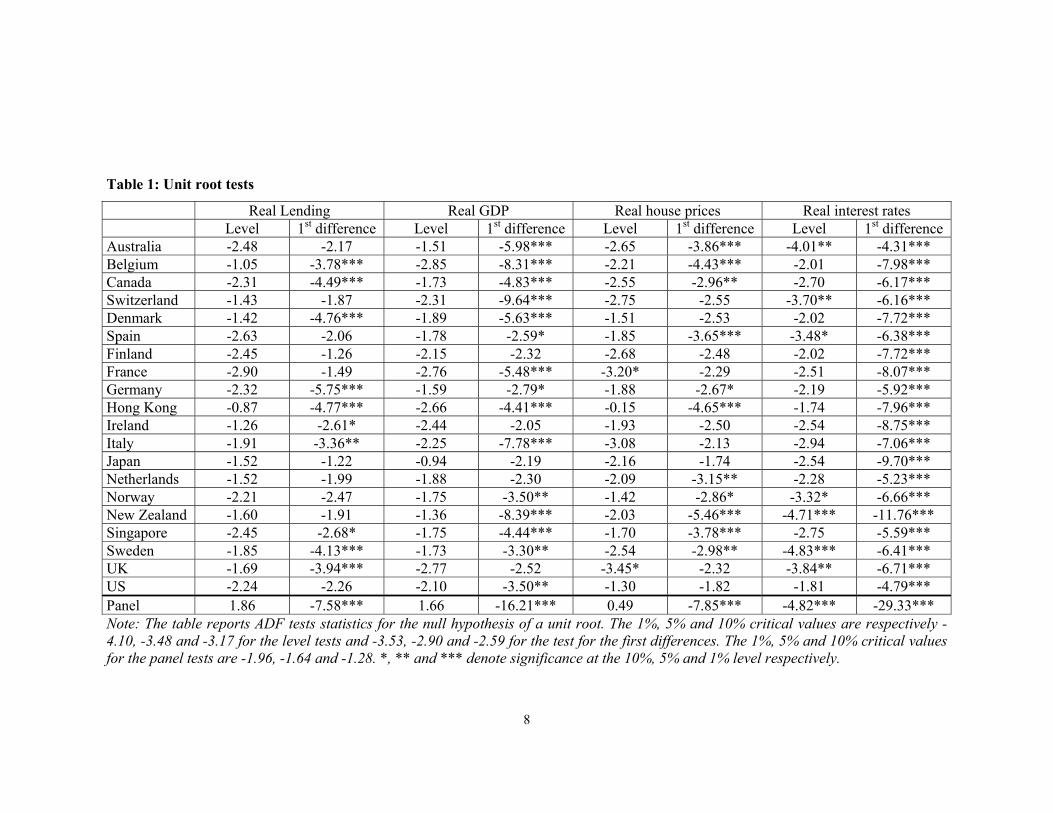
Table 1: Unit root tests
Real Lending Real GDP Real house prices Real interest rates Level 1st difference Level 1st difference Level 1st difference Level 1st difference Australia -2.48 -2.17 -1.51 -5.98*** -2.65 -3.86*** -4.01** -4.31*** Belgium -1.05 -3.78*** -2.85 -8.31*** -2.21 -4.43*** -2.01 -7.98*** Canada -2.31 -4.49*** -1.73 -4.83*** -2.55 -2.96** -2.70 -6.17*** Switzerland -1.43 -1.87 -2.31 -9.64*** -2.75 -2.55 -3.70** -6.16*** Denmark -1.42 -4.76*** -1.89 -5.63*** -1.51 -2.53 -2.02 -7.72*** Spain -2.63 -2.06 -1.78 -2.59* -1.85 -3.65*** -3.48* -6.38*** Finland -2.45 -1.26 -2.15 -2.32 -2.68 -2.48 -2.02 -7.72*** France -2.90 -1.49 -2.76 -5.48*** -3.20* -2.29 -2.51 -8.07*** Germany -2.32 -5.75*** -1.59 -2.79* -1.88 -2.67* -2.19 -5.92*** Hong Kong -0.87 -4.77*** -2.66 -4.41*** -0.15 -4.65*** -1.74 -7.96*** Ireland -1.26 -2.61* -2.44 -2.05 -1.93 -2.50 -2.54 -8.75*** Italy -1.91 -3.36** -2.25 -7.78*** -3.08 -2.13 -2.94 -7.06*** Japan -1.52 -1.22 -0.94 -2.19 -2.16 -1.74 -2.54 -9.70*** Netherlands -1.52 -1.99 -1.88 -2.30 -2.09 -3.15** -2.28 -5.23*** Norway -2.21 -2.47 -1.75 -3.50** -1.42 -2.86* -3.32* -6.66*** New Zealand -1.60 -1.91 -1.36 -8.39*** -2.03 -5.46*** -4.71*** -11.76*** Singapore -2.45 -2.68* -1.75 -4.44*** -1.70 -3.78*** -2.75 -5.59*** Sweden -1.85 -4.13*** -1.73 -3.30** -2.54 -2.98** -4.83*** -6.41*** UK -1.69 -3.94*** -2.77 -2.52 -3.45* -2.32 -3.84** -6.71*** US -2.24 -2.26 -2.10 -3.50** -1.30 -1.82 -1.81 -4.79*** Panel 1.86 -7.58*** 1.66 -16.21*** 0.49 -7.85*** -4.82*** -29.33*** Note: The table reports ADF tests statistics for the null hypothesis of a unit root. The 1%, 5% and 10% critical values are respectively -4.10, -3.48 and -3.17 for the level tests and -3.53, -2.90 and -2.59 for the test for the first differences. The 1%, 5% and 10% critical values for the panel tests are -1.96, -1.64 and -1.28. *, ** and *** denote significance at the 10%, 5% and 1% level respectively.
9
On the whole, the results suggest that the natural logs of real bank lending, real property
prices and real GDP are integrated of order one. This conclusion is suggested both by the
individual country level tests as well as by the panel tests. The short-term real interest rate
appears to be a borderline case. The null of non-stationarity is rejected at least at the 10%
level in seven countries out of 13 countries. The panel unit root test strongly suggests that the
real interest rate is a stationary process.
Given the results of the unit root tests we test in the following for the presence of a long-run
relationship between real bank lending, real GDP and real property prices. The level of the
real interest rate is not allowed to enter the long-run relationship. Since we have more than
two variables in the system and therefore potentially more than one long-run relationship
among these variables, the multivariate Johansen approach (Johansen, 1988, 1991, 1992),
which allows to test for the number of cointegrating relationships in the system, is a natural
starting point for cointegration analysis. The Johansen approach is based on maximum
likelihood estimation of a cointegrating VAR model, which can be formulated in vector error
correction form:
(3) ttktktt xxxx εµ ++Π+∆Γ++∆Γ=∆ −+−−− 11111 ..... .
where x is a vector of endogenous variables comprising the log of real bank lending, real GDP
and real property prices. µ is a vector of constants and ε is a vector of white noise error
terms. Since I want to allow for deterministic time trends in the levels of the data I leave the
constant µ unrestricted. The rank of the matrix Π indicates the number of long-run
relationships between the endogenous variables in the system11. The cointegrating rank
hypothesis for the Johansen trace test is specified as rrankrH ≤Π)(:)( against the
alternative prankpH =Π)(:)( .
The lag order of the VECMs was determined based on sequential Likelihood-ratio tests,
eliminating all lags up to the first lag significant at the 5% level. The results of the trace test
11 For a detailed technical exposition of the Johansen approach see Johansen (1995).

10
are reported in Table 2. The 1%, 5% and 10% critical values are respectively 35.65, 29.68
and 26.79 for 0)(:)0( =ΠrankH , 20.04, 15.41 and 13.33 for 1)(:)0( ≤ΠrankH and 6.65,
3.76 and 2.69 for 2)(:)0( ≤ΠrankH 12. I also report the result of a panel cointegration trace
test proposed by Larsson et al. (2001). The test statistic is the standardised average of the N
individual trace test statistics:
(4) δ
µ)( −=Ψ
LRNLR ,
where LR is the average of the individual trace test statistics and µ and δ are respectively
the mean and the variance of the asymptotic distribution of the trace test statistic, which are
tabulated in Osterwald-Lennum (1992). Larsson et al. (2001) show that the test statistic has a
standard normal distribution. The test is one sided with large positive values of the test
statistics suggesting a rejection of the null hypothesis of no cointgration. The 1%, 5% and
10% critical values are therefore 1.96, 1.64 and 1.28 respectively.
The results suggest that there is a single long-run relationship between bank lending, GDP
and property prices. The null of no cointegration is rejected at least at the 10% level in 15 out
of 20 countries. Two long-run relationships are indicated only for the UK. The panel trace test
rejects the null hypothesis of one long-run relationship against the alternative of no long-run
relationship, but it does not reject the null hypothesis of one long-run relationship against the
alternative of more than one, therefore suggesting that there is a single long-run relationship
in the system.
In order to cross-check the results of the Johansen test I also report in Table 2 the results of
two alternative residual based cointegration tests. Residual based cointegration tests were first
discussed in Engle and Granger (1987) and are based on tests of a unit root hypothesis in the
residuals tε̂ of the estimated cointegrating relationship
(6) tttt xxy εββα ˆˆˆˆˆ 2211 +++= ,
12 Critical values were taken from Osterwald-Lennum (1992).
11
where in our case y is the log of real bank lending, 1x is the log of real GDP and 2x is the log
of real property prices. I calculate the long-run residuals tε̂ based on the dynamic OLS
(DOLS) estimator of the long-run coefficients proposed by Saikkonen (1991) and Stock and
Watson (1993), which controls for regressor endogeneity and serial correlation in the long-run
regression by adding leads and lags of the first difference of the regressors to the estimating
equation. I then apply a standard ADF unit root test and a Lagrange multiplier (LM) test
proposed by Harris and Inder (1994). The former tests the null of no cointegration, while the
latter takes cointegration as the null.
The ADF cointegration test regression is given by:
(6) ∑=
−− +∆++=∆k
itittt
11 ˆˆˆ ςεεγµε
The lag order k was determined by sequential t-tests eliminating all lags up to the first
significant at the 5% level, allowing for a maximum lag order of four. The 1%, 5% and 10%
critical values were calculated based on the response surfaces reported in MacKinnon (1991)
and are respectively -4.50, -3.86 and -3.54. I also report a panel ADF cointegration test
proposed by Pedroni (1999). The test statistic is the standardised average of the N individual
ADF cointegration test statistics:
(7) δ
µγ )( −=Ψ
tNADF ,
which has again a standard normal distribution. The test is again one sided with large negative
values suggesting a rejection of the null. The results, which are reported in the second-last
column of Table 2, clearly suggest that the null of no cointegration cannot be rejected. Not a
single test statistic is statistically significant.
The LM test proposed by Harris and Inder (1994) is a multivariate extension of the unit root
test proposed by Kwiatkowski et al. (1992). The test statistic is given by:

12
(8) 21
2
ˆεσ
∑==
T
ttS
LM
where ∑ == ti itS 1
2 ε̂ is the running partial sum of the residuals and εσ̂ is the estimated residual
variance. The 1%, 5% and 10% critical values are respectively 0.37, 0.22 and 0.16 (Harris and
Inder, 1994). McCoskey and Kao (1998) proposed a panel version of the Harris and Inder
cointegration test. The test statistic is the standardised average of the N individual LM test
statistics:
(9) δ
µ)( −=Ψ
LMNLM .
This test statistic is again one sided with a standard normal distribution. Large positive values
suggest a rejection of the null. The test results are reported in the last column of Table 2 and
suggest that the null of cointegration cannot be rejected for about half of the countries and
also not by the panel test.
What do we make of these results? The Johansen and the Harris and Inder test suggest that
there exists a (single) long-run relationship linking bank lending, GDP and property prices,
while the ADF cointegration test suggests that there is no cointegration. Monte Carlo
evidence on the performance of cointegration tests in small samples, which is summarised in
Maddala and Kim (1998), appears to be inconclusive on which test is more reliable. A priori it
is therefore unclear which test we should trust more. The cointegration test results do not
provide compelling evidence in favour of cointegration, but neither do they provide
compelling evidence against it. With a view to the following section, the main conclusion of
this section is therefore that cointegration tests do not make a clear case against the inclusion
of a long-run relationship between bank lending and property prices in dynamic models of
bank lending and property price interaction.

13
Table 2: Cointegration Test Results
Johansen Test Residual Based Tests 0=r 1≤r 2≤r ADF test LM test Australia 30.48** 9.37 0.74 -2.55 0.14 Belgium 28.5* 8.64 0.42 -1.31 0.19 Canada 27.78* 8.33 0.05 -1.68 0.24** Switzerland 27.45* 9.92 1.7 -0.74 0.20* Denmark 22.94 8.26 0.84 -1.78 0.22** Spain 35.72*** 8.29 0.49 -1.11 0.15 Finland 54.24*** 13.29 0.48 -1.81 0.24** France 32.45** 10.03 0.68 -0.78 0.22** Germany 30.58** 8.73 1.12 -2.52 0.24** Hong Kong 21.13 6.31 0.01 -3.44 0.07 Ireland 25.41 4.76 0.56 -2.56 0.13 Italy 19.22 4.24 0.07 -1.56 0.11 Japan 53.36*** 11.19 1.75 -3.47 0.08 Netherlands 20.88 5.1 0.14 -2.88 0.18* Norway 48.58*** 11.22 5.27 -1.72 0.2 New Zealand 26.96* 9.63 2.99 -2.78 0.17 Singapore 28.48* 3.82 0.1 -3.35 0.11 Sweden 31.05** 13.37 1.92 -2.58 0.24** UK 38.41*** 18.70** 2.95 -1.51 0.23** US 29.49* 10.75 0.34 -2.18 0.19* Panel 9.69*** 1.14 0.44 -0.70 1.02
Note: ‘Johansen test’ displays the test statistics of the Johansen trace test for cointegration. The 1%, 5% and 10% critical values for the cointegration test are 35.65, 29.68 and 26.79 for r=0, 20.04, 15.41 and 13.33 for 1≤r and 6.65, 3.76 and 2.69 for 2≤r (Osterwald-Lennum, 1992). The 1%, 5% and 10% critical values for the panel cointegration test are respectively 1.96, 1.64 and 1.28. ‘ADF test’ reports the ADF cointegration test statistic. The 10% critical value is -3.54 for the individual country tests and -1.28 for the panel test. ‘LM test’ reports the results of the Harris and Inder cointegration test. The 1%, 5% and 10% critical values are 0.37, 0.22 and 0.16 for the individual country tests. The 10% critical value for the panel test is 1.28. *, ** and *** indicates significance of a test statistic at the 10%, 5% and 1% level respectively.
14
As the next step we proceed to estimate the long-run coefficients linking real bank lending,
real GDP and real property prices. Since we have at most one long-run relationship there are
various approaches that are applicable. In Table 3 we present estimates from the Johansen
Maximum Likelihood procedure, which are obtained by imposing identifying restrictions on
the cointegrating vector. We also report estimates obtained from the Fully Modified OLS
(FM-OLS) approach proposed by Phillips and Hansen (1990) and from the DOLS approach
proposed by Saikkonen (1991) and Stock and Watson (1993). The former controls for
regressor endogeneity and serial correlation by applying a non-parametric correction to the
OLS estimators of the long-run coefficients in (6), while the latter adds leads and lags of the
first difference of the regressors to the long-run regression equation. For both the FM-OLS
and the DOLS estimator we also report panel estimates based on fixed effects panel
estimators proposed respectively by Pedroni (1999) and Kao and Chiang (2000).
For each estimator we report the coefficient estimates with t-statistics in parentheses. The
results suggest that in most countries real GDP and real property prices both enter
significantly the cointegrating vector. However, while the estimates obtained from the FM-
OLS and the DOLS estimators are broadly similar, the estimates obtained from the Johansen
procedure are sometimes quite different and counter-intuitive. Monte Carlo studies,
summarised in Maddala and Kim (1998), suggest that the Johansen procedure exhibits larger
variation than single equation estimators in small samples. The Monte Carlo evidence also
suggests that the DOLS approach is preferable to the FM-OLS estimator in small samples.
Kao and Chiang (2000) report Monte Carlo evidence suggesting that also the panel DOLS
estimator outperforms the panel FM-OLS estimator in small samples. For this reason, the
error-correction terms which are included in the error-correction models estimated in the
following section were calculated using the DOLS estimates of the long-run coefficients.

15
Table 3: Long-run Relationships
Johansen ML Fully Modified OLS Dynamic OLS Real GDP Real house
prices Real GDP Real house
prices Real GDP Real house
prices Australia 1.97
(11.16) -0.78
(-2.76) 1.34
(12.10) 0.40
(2.58) 1.41
(12.55) 0.33
(1.92) Belgium 2.67
(2.61) -2.77
(-4.89) 0.24
(0.40) 0.97
(3.00) 0.49
(0.83) 0.85
(2.78) Canada 1.37
(13.38) 0.002 (0.02)
1.42 (15.40)
0.26 (2.13)
1.40 (18.11)
0.28 (4.41)
Switzerland 4.90 (6.46)
0.12 (0.43)
1.92 (11.83)
0.16 (2.49)
2.06 (10.97)
0.19 (3.77)
Denmark 0.80 (2.26)
0.47 (1.89)
0.65 (1.75)
0.24 (1.07)
0.75 (4.38)
0.19 (1.47)
Spain 2.66 (11.18)
-0.56 (-5.03)
1.99 (11.70)
-0.02 (-0.21)
2.04 (12.98)
-0.10 (-0.94)
Finland -0.31 (-1.62)
1.41 (8.64)
0.02 (0.06)
0.32 (1.43)
0.23 (0.71)
0.23 (1.31)
France 0.83 (15.12)
0.92 (13.55)
0.94 (8.86)
0.78 (5.84)
0.95 (26.43)
(0.88 (19.23)
Germany 2.17 (36.06)
-0.69 (-9.86)
2.23 (26.72)
-0.47 (-5.67)
2.22 (66.39)
-0.46 (-8.63)
Hong Kong 2.17 (6.18)
0.001 (0.01)
1.27 (12.96)
0.21 (3.17)
1.31 (13.34)
0.18 (3.06)
Ireland 1.12 (8.74)
0.79 (6.29)
0.95 (10.35)
0.84 (9.05)
0.89 (16.41)
0.88 (19.04)
Italy 2.04 (1.91)
2.36 (3.66)
2.05 (14.32)
0.24 (3.05)
1.98 (26.22)
0.25 (4.49)
Japan 2.73 (12.84)
0.47 (2.49)
1.13 (32.90)
0.53 (12.88)
1.20 (44.03)
0.56 (26.56)
Netherlands 0.26 (1.42)
1.03 (10.09)
0.54 (3.17)
0.87 (10.21)
0.46 (3.11)
0.93 (12.12)
Norway 1.48 (49.04)
0.77 (9.56)
1.57 (9.05)
0.39 (2.76)
1.59 (35.61)
0.44 (7.26)
New Zealand 1.32 (2.69)
0.90 (2.04)
2.12 (7.24)
0.05 (0.17)
1.82 (6.72)
0.28 (1.45)
Singapore 0.83 (16.61)
0.24 (5.34)
0.92 (8.98)
0.14 (1.56)
0.91 (16.83)
0.17 (3.79)
Sweden 0.74 (1.44)
-0.42 (-1.11)
0.42 (1.63)
0.78 (5.14)
0.58 (2.14)
0.78 (6.00)
UK 1.82 (13.53)
0.35 (3.27)
1.98 (9.88)
0.26 (1.69)
1.98 (19.47)
0.35 (2.99)
US 1.49 (25.07)
1.67 (6.79)
1.63 (16.50)
0.97 (3.44)
1.63 (38.43)
1.07 (6.92)
Panel - - 1.27 (48.25)
0.40 (14.71)
1.22 (11.15)
0.26 (5.12)

16
4. Dynamic Interaction
In this section I estimate error-correction models (ECMs) for credit growth and the change in
property prices in order to investigate the patterns of long-run and short-run causality between
bank lending and property prices. The ECMs are of the form:
(10) tttti
ititt rpylCIl εγγγγγ +∆+∆+∆+∆+=∆ −=
−− ∑ 1432
4
0110
(11) tttti
ititt rlypCIp υλλλλλ +∆+∆+∆+∆+=∆ −=
−− ∑ 1432
4
0110 ,
where l∆ is real lending growth, y∆ is real GDP growth, p∆ is the change in real property
prices and r∆ is the change in the short-term real interest rate. CI is the DOLS estimate of the
cointegrating vector linking the levels of real bank lending, real GDP and real property prices
reported in Table 3. Estimating equation (10) and (11) for 20 countries yields two systems of
20 equations each for the change in real lending and the change in real property prices. In
order to prevent simultaneity bias from affecting the estimation the contemporaneous
variables included in each equation were instrumented for using four own lags as instruments.
The systems were estimated by three stage least squares in order to account for potential
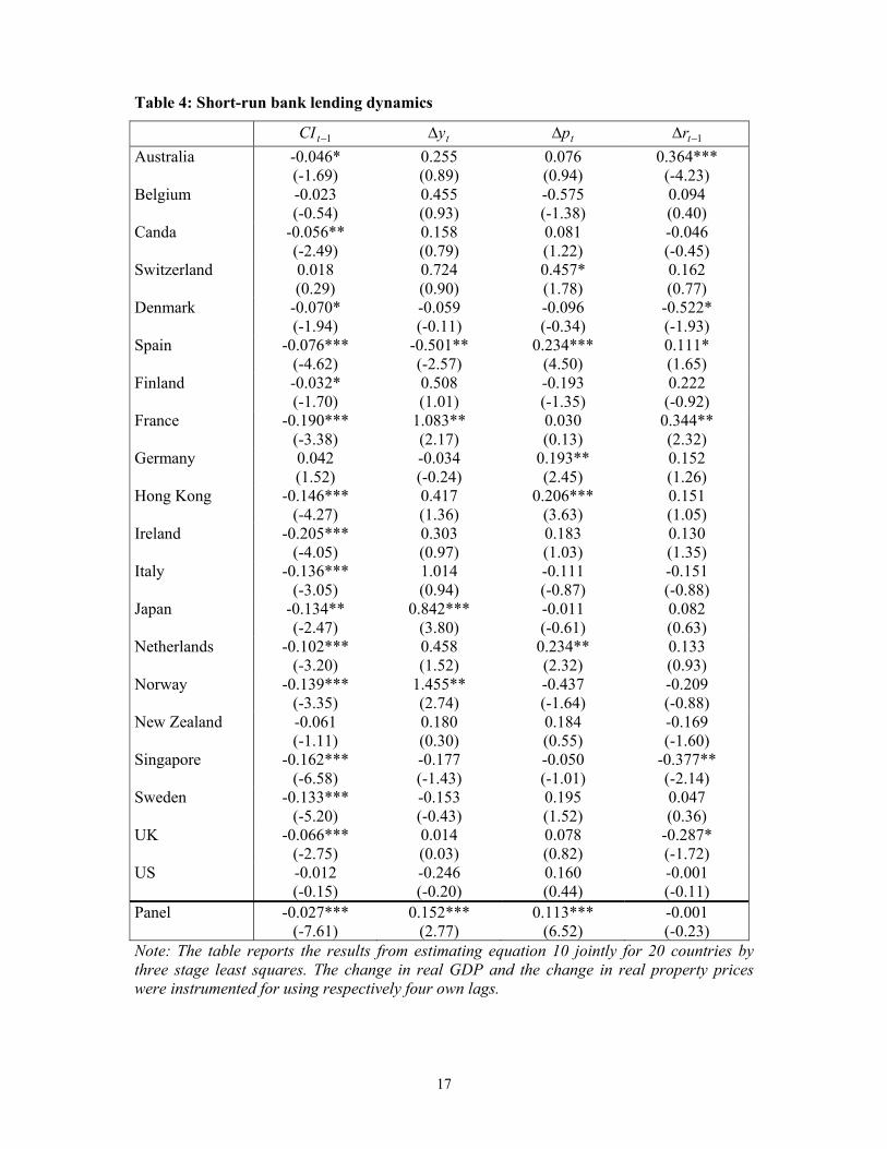
contemporaneous correlation in the errors across equations. Tables 4 and 5 report the
estimation results. Coefficients are reported with t-statistics in parentheses. The last row
reports the results of a pooled fixed effects three-stage least squares regression.
17
Table 4: Short-run bank lending dynamics
1−tCI ty∆ tp∆ 1−∆ tr Australia -0.046*
(-1.69) 0.255 (0.89)
0.076 (0.94)
0.364*** (-4.23)
Belgium -0.023 (-0.54)
0.455 (0.93)
-0.575 (-1.38)
0.094 (0.40)
Canda -0.056** (-2.49)
0.158 (0.79)
0.081 (1.22)
-0.046 (-0.45)
Switzerland 0.018 (0.29)
0.724 (0.90)
0.457* (1.78)
0.162 (0.77)
Denmark -0.070* (-1.94)
-0.059 (-0.11)
-0.096 (-0.34)
-0.522* (-1.93)
Spain -0.076*** (-4.62)
-0.501** (-2.57)
0.234*** (4.50)
0.111* (1.65)
Finland -0.032* (-1.70)
0.508 (1.01)
-0.193 (-1.35)
0.222 (-0.92)
France -0.190*** (-3.38)
1.083** (2.17)
0.030 (0.13)
0.344** (2.32)
Germany 0.042 (1.52)
-0.034 (-0.24)
0.193** (2.45)
0.152 (1.26)
Hong Kong -0.146*** (-4.27)
0.417 (1.36)
0.206*** (3.63)
0.151 (1.05)
Ireland -0.205*** (-4.05)
0.303 (0.97)
0.183 (1.03)
0.130 (1.35)
Italy -0.136*** (-3.05)
1.014 (0.94)
-0.111 (-0.87)
-0.151 (-0.88)
Japan -0.134** (-2.47)
0.842*** (3.80)
-0.011 (-0.61)
0.082 (0.63)
Netherlands -0.102*** (-3.20)
0.458 (1.52)
0.234** (2.32)
0.133 (0.93)
Norway -0.139*** (-3.35)
1.455** (2.74)
-0.437 (-1.64)
-0.209 (-0.88)
New Zealand -0.061 (-1.11)
0.180 (0.30)
0.184 (0.55)
-0.169 (-1.60)
Singapore -0.162*** (-6.58)
-0.177 (-1.43)
-0.050 (-1.01)
-0.377** (-2.14)
Sweden -0.133*** (-5.20)
-0.153 (-0.43)
0.195 (1.52)
0.047 (0.36)
UK -0.066*** (-2.75)
0.014 (0.03)
0.078 (0.82)
-0.287* (-1.72)
US -0.012 (-0.15)
-0.246 (-0.20)
0.160 (0.44)
-0.001 (-0.11)
Panel -0.027*** (-7.61)
0.152*** (2.77)
0.113*** (6.52)
-0.001 (-0.23)
Note: The table reports the results from estimating equation 10 jointly for 20 countries by three stage least squares. The change in real GDP and the change in real property prices were instrumented for using respectively four own lags.

18
Table 5: Short-run property price dynamics
1−tCI ty∆ tl∆ 1−∆ tr Australia 0.151***
(3.18) -0.425 (-0.62)
0.467*** (2.77)
-0.570*** (-2.94)
Belgium 0.119*** (3.55)
-0.595 (-1.05)
0.577* (1.92)
-0.397 (-1.58)
Canda -0.014 (-0.17)
-0.262 (-0.41)
0.269 (0.50)
-0.450** (-2.01)
Switzerland 0.003 (0.05)
0.186 (0.22)
-0.007 (-0.02)
-0.289 (-1.26)
Denmark -0.081*** (-3.74)
-0.203 (-0.61)
0.168 (1.55)
-0.414* (-2.45)
Spain 0.016 (0.40)
-0.723 (-1.21)
0.244 (1.22)
-0.062 (-0.36)
Finland -0.075** (-2.20)
-1.426** (-1.83)
-0.264 (-1.01)
-0.705*** (-2.76)
France -0.027 (-0.51)
-0.162 (-0.54)
0.207 (1.00)
-0.115 (-1.03)
Germany -0.186*** (-5.03)
0.515** (2.68)
0.211 (0.81)
-0.388*** (-2.87)
Hong Kong 0.208* (1.71)
0.773 (1.14)
0.840 (1.45)
-0.186 (-0.39)
Ireland 0.011 (0.10)
1.600*** (4.36)
0.378 (0.89)
-0.127 (-0.90)
Italy 0.025 (0.48)
2.310* (1.65)
0.620** (2.03)
0.068 (0.29)
Japan 0.019 (0.35)
0.427** (2.10)
0.242* (1.78)
0.092 (0.81)
Netherlands 0.234*** (4.77)
0.541 (1.25)
0.532** (2.52)
-0.538*** (-2.63)
Norway -0.022 (-0.29)
-0.015 (-0.03)
0.576* (1.77)
-0.514* (-1.99)
New Zealand -0.04 (-0.81)
0.487 (1.18)
0.018 (0.10)
-0.233** (-2.09)
Singapore -0.241 (-1.58)
1.389** (2.64)
-0.110 (-0.21)
-0.354 (-0.569)
Sweden -0.007 (-0.24)
-0.354 (-1.28)
-0.057 (-0.43)
-0.246** (-2.31)
UK -0.015 (-0.25)
2.349*** (3.00)
0.569 (1.56)
-0.542* (-1.70)
US 0.073*** (4.04)
-0.251 (-0.85)
-0.095 (-1.39)
0.054 (0.41)
Panel -0.003 (-0.71)
0.475*** (6.07)
0.136*** (3.99)
-0.241*** (-6.74)
Note: The table reports the results from estimating equation 11 jointly for 20 countries by three stage least squares. The change in real GDP and the change in real lending were instrumented for using respectively four own lags.

19
The results suggest that long-run causality goes from property prices to bank lending, rather
than conversely. The error-correction term in the ECM for bank lending is significantly
negative in 15 out of 20 cases and the panel estimate is significantly negative at the 1% level.
In the ECM for property prices, the error-correction term is significantly positive in 5 cases,
but significantly negative in three. The pooled estimate is insignificant. Short-run causality
appears to go in both directions. The change in real property prices (real bank lending) has a
significantly positive effect on bank lending (property prices) in five (six) countries and the
pooled estimate is in both ECMs significant at the 1% level. GDP growth and real interest
rates appear to matter more for property prices than for bank lending. GDP growth has a
significantly positive effect on property prices (bank lending) in 3 (6) countries. The pooled
estimate is in both cases significantly positive at the 1% level. The change in real interest rates
has a significantly negative effect on property prices (bank lending) in 10 (2) countries. The
pooled estimate is significantly negative at the 1% level in the property prices ECM but
insignificant in the bank lending ECM13.
5. Conclusions
Over the last couple of years, the coincidence of cycles in credit and property markets has
been widely documented and discussed in the policy oriented literature. In this paper I
analyse the causes of this coincidence. From a theoretical point of view, the relationship
between bank lending and property prices is multifaceted. Property prices may affect credit
via various wealth effects, while credit may affect property prices via various liquidity
effects. Previous empirical studies were not able to disentangle the direction of causality,
since the focus was usually on either effect, but not on both.
13 The finding of bank lending being rather irresponsive to interest rates is consistent with the results of the impulse response analysis in Goodhart and Hofmann (2003).

20
I analyse the patterns of dynamic interaction between bank lending and property prices based
on a sample of 20 industrialised countries using both time series and panel data techniques.
Long-run causality appears to go from property prices to bank lending, rather than
conversely. This finding suggests that property price cycles, reflecting changing beliefs about
future economic prospects, drive credit cycles, rather than excessive bank lending, in the
wake of financial liberalization or overly loose monetary policy, being the cause of property
price bubbles. However, there is also evidence of short-run causality going in both directions,
implying that a mutually re-enforcing element in past boom bust cycles in credit and property
markets cannot be ruled out.
21
References
Ando, A. and F. Modigliani (1963). The ‘Life Cycle’ Hypothesis of Saving: Aggregate
Implications and Tests. American Economic Review, 53, 55-84.
Bernanke, B. and M. Gertler (1989). Agency Costs, Collateral and Business Fluctuations.
American Economic Review, 79, 14-31.
Bernanke, B., M. Gertler and S. Gilchrist (1998). The Financial Accelerator in a Quantitative
Business Cycle Framework. NBER Working Paper No. 6455.
BIS (1999). The Monetary and Regulatory Implications of Changes in the Banking Industry.
BIS Conference Papers No.7.
BIS (2001), 71st Annual Report.
Borio, C. and W. Fritz (1995). The Response of Short-Term Bank Lending Rates to policy
Rates: A Cross-Country Perspective. BIS Working Paper No. 27.
Borio, C., N. Kennedy and S. Prowse (1994). Exploring Aggregate Asset Price Fluctuations
across Countries: Measurement, Determinants and Monetary Policy Implications.
Bank for International Settlements. BIS Working Paper No. 40.
Deaton, A. (1992). Understanding Consumption. Oxford University Press.
Dickey, D. and W. Fuller (1981). Likelihood Ratio Statistics for Autoregressive Time Series
with a Unit Root. Econometrica, 60, 423-433.
Drees, B. and C. Pazarbasioglu (1998). The Nordic Banking Crises. Pitfalls in Financial
Liberalization? IMF Occasional Paper No. 161.

22
Engle, R. and C. Granger (1987). Cointegration and Error-correction: Representation,
Estimation and Testing. Econometrica, 55, 252-276.
Fisher, I. (1933). The Debt-Deflation Theory of Great Depressions. Econometrica, 1, 337-57.
Gerlach, S. and W. Peng (2003). Bank Lending and Property Prices in Hong Kong. HKIMR
Working Paper No. 12/2003.
Goodhart, C. (1995). Price Stability and Financial Fragility. In: K. Sawamoto, Z. Nakajima
and H. Taguchi (Eds.). Financial Stability in a Changing Environment. St. Martin’s
Press.
Goodhart, C. and B. Hofmann (2003). Deflation, Credit, and Asset Prices. Forthcoming in:
P. Siklos and R. Burdekin, The Anatomy of Deflation, Cambridge University Press
Harris, D. and B. Inder (1994). A Test for the Null of Cointegration. In: C. Hargreaves (ed.),
Non-stationary Time-series Analysis and Cointegration. Oxford University Press, Oxford,
133-152.
Hofmann, B. (2001). The Determinants of Private Sector Credit in Industrialised Countries:
Do Property Prices Matter?, BIS Working Paper No. 108.
Hofmann, B. (2002). The Pass-Through of Money Market Rates to Loan Rates in the Euro-
Area. Mimeo, ZEI, University of Bonn.
Hofmann, B. and P. Mizen (2002). Base Rate Pass-Through in UK Banks’ and Building
Societies’ Retail Rates. Bank of England Working Paper No. 117.
Hofmann, B. and P. Mizen (2003). Interest Rate Pass-Through and Monetary Transmission:
Evidence from Individual Financial Institutions’ Retail Rates, Economica,
forthcoming.

23
Hoshi, T. and A. Kashyap (1999). The Japanese Banking Crisis: Where Did it Come from and
How Will it End? NBER Working Paper No. 7250.
Im, K., H. Pesaran and Y. Shin (2003). Testing for Unit Roots in Heterogeneous Panels.
Journal of Econometrics, 115, 53-74.
IMF (2000). World Economic Outlook, May 2000.
Johansen, S. (1988). Statistical Analysis of Cointegration Vectors. Journal of Economic
Dynamics and Control, 12, 231-54.
Johansen, S. (1991). Estimation and Hypothesis Testing of Cointegration Vectors in Gaussian
Vector Autoregressive Models. Econometrica, 59, 1551-1580.
Johansen, S. (1992). Detzermination of Cointegration Rank in the Presence of a Linear Trend.
Oxford Bulletin of Economics and Statistics, 54, 383-397.
Johansen, S. (1995). Likelihood-Based Inference in Cointegrated Vector Autoregressive
Models. Oxford University Press.
Kao, C. and M. Chiang (2000). On the Estimation and Inference of a Cointegrated Regression
in Panel Data. Advances in Econometrics, 15, 179-222.
Keynes, J. (1931). The Consequences for the Banks of the Collapse in Money Values. In:
Essays in Persuasion, Macmillan.
Kindleberger, C. (1978). Manias, Panics and Crashes: A History of Financial Crises. In: C.
Kindleberger and J. Laffarge (Eds.) Financial Crises: Theory, History and Policy,
Cambridge University Press.
Kiyotaki, N. and J. Moore (1997). Credit Cycles. Journal of Political Economy, 105, 211-248.

24
Kwiatkowski, D., P. Phillips, P. Schmidt and Y. Shin (1992). Testing the Null Hypothesis of
Stationarity against the Alternative of a Unit Root. Journal of Econometrics, 54, 159-
178.
Larsson, R., J. Lyhagen and M. Löthgren (2001). Likelihood-based Cointegration Tests in
Heterogeneous Panels. Econometrics Journal, 4, 109-142.
McCoskey, S. and C. Kao (1998). A Residual Based Test of the Null of Cointegration in
Panel Data. Econometric Reviews, 17, 57-84.
Maddala, G. and I. Kim (1998). Unit Roots, Cointegration, and Structural Change. Cambridge
University Press, Cambridge.
Minsky, H. (1982), ‘Can ‘’It’’ happen again?’, Essays on Instability and Finance, M.E. Sharpe
Muellbauer, J. (1994). The Assessment: Consumer Expenditure. Oxford Review of Economic
Policy, 10, 1-41.
OECD (2000), Economic Outlook 68, December 2000.
Osterwald-Lenum, M. (1992). A Note with Quantiles of the Asymptotic Distribution of the
Maximum Likelihood Cointegration Rank Test Statistics, Oxford Bulletin of
Economics and Statistics, 54, 461-472.
Pedroni, P. (1999). Critical Values for Cointegration Tests in Heterogeneous Panels with
Multiple Regressors. Oxford Bulletin of Economics and Statistics, 61, 653-670.
Pedroni, P. (2000). Fully Modified OLS for Heterogeneous Cointegrated Panels. Advances in
Econometrics, 15, 93-130.
Phillips, P. and B. Hansen (1988). Statistical Inference in Instrumetal Variables Regression
with I(1) Processes. Review of Economic Studies, 57, 99-125.

25
Saikkonen, P. (1991). Asymptotically Efficient Estimation of Cointegrating Regressions.
Econometric Theory, 7, 1-21.
Stock, J. and M. Watson (1993). A simple Estimator of Cointegrating Vectors in Higher
Order Integrated Systems. Econometrica, 61, 783-820.


