analyisis of scoring in peer-to- peer lending...peer-to-peer-lending (also known as person-to-person...
TRANSCRIPT
ANALYISIS OF SCORING IN PEER-TO-
PEER LENDING DETERMINANTS OF LOAN DEFAULT
Aantal woorden/ Word count: 12.659
Davy Lust Stamnummer/ Student number : 01201013
Promotor/ Supervisor: Prof. dr. Rudi Vander Vennet
Masterproef voorgedragen tot het bekomen van de graad van:
Master’s Dissertation submitted to obtain the degree of:
Master of Science in Business Engineering
Academiejaar/ Academic year: 2016 - 2017

VERTROUWELIJKHEIDSCLAUSULE/ CONFIDENTIALITY AGREEMENT
PERMISSION
Ondergetekende verklaart dat de inhoud van deze masterproef mag geraadpleegd en/of
gereproduceerd worden, mits bronvermelding.
I declare that the content of this Master’s Dissertation may be consulted and/or reproduced,
provided that the source is referenced.
Naam student/name student:
Davy Lust
Handtekening/signature
II
Dutch summary
Deze thesis is gericht op het bepalen van de kredietwaardigheid van een ontlener in de peer-
to-peer-leningenmarkt. Hierbij wordt in de eerste plaats aandacht besteed aan het bepalen van
de voornaamste determinanten van een ‘loan default’, of de situatie waarbij de ontlener niet
meer aan zijn financiële verplichtingen kan voldoen. Om dit te doen, maken we gebruik van
een dataset van het grootste Amerikaanse P2P-Lending platform, namelijk Lending Club.
Hierin zijn alle gegevens met betrekking tot de op het platform uitgegeven leningen terug te
vinden. Aan de hand van deze dataset stellen we een statistisch model op, dat de status van de
lening (default of niet) op het eind van de looptijd relateert aan de verschillende gegevens met
betrekking tot de ontlener, zoals bijvoorbeeld zijn inkomen, huidige schulden en
betalingsverleden. Op die manier kan worden vastgesteld welke variabelen een invloed
uitoefenen op het zich al dan niet voordoen van een loan default, en hoe deze variabelen aan
deze waarschijnlijkheid zijn gerelateerd.
De thesis vangt aan met een beschrijving van het concept ‘peer-to-peer lending’, waarbij ook
de voor- en nadelen voor zowel de ontlener als de investeerder worden besproken. Vervolgens
wordt de huidige situatie op de Europese, Amerikaanse en Aziatische P2P-Lending markt
besproken, en wordt er dieper ingegaan op hoe ‘credit scoring’ in deze financiële markten
doorgaans in z’n werk gaat.
De paper gaat verder met het beschrijven van de gebruikte data, en hoe deze data is verwerkt
om in het statistisch model opgenomen te kunnen worden. Hierna wordt dieper ingegaan op
het toegepaste statistische model, meer bepaald het logit model, de karakteristieken van dit
model, en welke invloed dit heeft op onze analyse.
Ten slotte worden de resultaten van het onderzoek weergegeven. Deze resultaten worden
vergeleken met de huidige literatuur rond ‘credit scoring’, alsook met gelijkaardige studies, om
zinvolle conclusies te kunnen trekken. Verder worden er voor elk van de bevindingen
economisch gerelateerde verklaringen gezocht.

III
Foreword
This master’s dissertation serves as the conclusion of five years of intensive academic and
personal development, and is the final stepping stone towards a promising future as a graduate
in Business Engineering.
I would like to take this opportunity to first of all thank my parents for their continuous
support, both mentally and financially, during this important period in my life. Secondly, I
want to thank prof. dr. Rudi Vander Vennet, for granting me the opportunity to work on this
fascinating and challenging topic, as well as Thomas Present, for his excellent guidance during
the development of this thesis. Finally, I want to express my heartfelt gratitude towards my
girlfriend, for her everlasting motivation and continuous belief in me.

IV
Table of content
Dutch summary ......................................................................................................................... II
Foreword .................................................................................................................................. III
Table of content ........................................................................................................................ IV
List of used abbreviations ........................................................................................................ VI
List of Figures and Tables ....................................................................................................... VII
1 Introduction ......................................................................................................................... 1
2 Theoretical Background ...................................................................................................... 2
2.1 What is Peer-To-Peer-Lending? .................................................................................. 2
2.2 Advantages of P2P-Lending ........................................................................................ 2
2.2.1 Advantages for the lender ........................................................................................ 3
2.2.2 Advantages for the borrower ................................................................................... 3
2.3 Disadvantages of P2P-Lending ................................................................................... 4
2.4 Market overview .......................................................................................................... 5
2.4.1 American market - USA ........................................................................................... 5
2.4.2 Asian market ............................................................................................................ 6
2.4.3 European market ..................................................................................................... 6
2.5 Credit Scoring .............................................................................................................. 7
2.5.1 Credit Scoring in general ......................................................................................... 7
2.5.2 Credit Scoring in P2P-Lending ................................................................................ 8
3 Data Description ............................................................................................................... 10
3.1 Data set and variables ................................................................................................ 10
3.1.1 Dependent variable .................................................................................................12
3.1.2 Predictor variables ..................................................................................................12
3.2 Descriptive statistics and correlation matrix ............................................................. 15
4 Econometrical Methodology .............................................................................................. 17
4.1 Model selection ........................................................................................................... 17
4.2 Model characteristics ................................................................................................. 18

V
4.2.1 Goodness of Fit .......................................................................................................19
4.2.2 Model significance ................................................................................................. 20
4.2.3 Significance of variables ........................................................................................ 20
4.2.4 Coefficient interpretation .......................................................................................21
5 Specification Adjustments ................................................................................................ 22
5.1 Employment length ................................................................................................... 22
5.2 Open Accounts & Total Accounts .............................................................................. 23
5.3 Public records & Months since last record ................................................................ 23
6 Empirical Results .............................................................................................................. 26
6.1 Non-significant variables .......................................................................................... 26
6.2 Significant variables .................................................................................................. 28
7 Conclusion ........................................................................................................................ 33
8 Further Research .............................................................................................................. 34
References ................................................................................................................................... I
Appendices ............................................................................................................................... IV

VI
List of used abbreviations
Abbreviation
Meaning
P2P-Lending Peer-To-Peer Lending
EU European Union
USA United States of America
UK United Kingdom
SME Small and Medium-sized Enterprises
FICO Fair Isaac Corporation
DTI Debt-To-Income
LC Lending Club
LPM Linear Probability Model
MLE Maximum Likelihood Estimation
LR Likelihood Ratio
OLS Ordinary Least Squares

VII
List of Figures and Tables
Figure 1: FICO-score Components ............................................................................................. 8
Figure 2: VantageScore 3.0 Influences ...................................................................................... 9
Table 1: Model Variables and Description ................................................................................ 11
Table 2: Descriptive statistics of numerical variables ............................................................... 15
Table 3: Correlation matrix of numerical variables ..................................................................16
Table 4: Regression results initial model - coefficients and odds ratios...................................19
Figure 3: Regression coefficients employment length, including linear trendline .................. 22
Table 5: Regression results Final Model .................................................................................. 24
Table 6: Regression coefficients for different specifications ................................................... 25

1
1 Introduction
In today’s ever changing, global society where individualism and self-interest are frowned
upon, and the prosperity of the community and the globe is becoming a core value in the policy
of the future, we can observe the emergence of all kinds of social initiatives. This is also the
case in the financial market, where actors often happily exchange the lack of connectedness or
the institutional and authoritarian structures of mainstream financial institutions for more
social, transparent and relational alternatives (Hulme & Wright, 2006). The emergence of
social lending is a clear example of this current trend.
The main part of this paper aims at analysing the scoring of loans in the peer-to-peer lending
market, based on data provided by Lending Club. This data is used to develop a model relating
the probability of default of borrowers to personal information provided during the loan
application, in order to define the main determinants of loan default in the P2P-Lending
market.
In the first part of this paper, we shortly introduce the concept of P2P-Lending, its
characteristics, advantages and disadvantages compared to traditional investment or
borrowing opportunities, and the influences on the financial market. This allows us to
determine the need for adequate credit scoring in social lending. We further describe the
emergence of P2P-Lending in the financial market, followed by an overview of the American,
Asian and European P2P-Lending markets.
The paper continues with a description and interpretation of the data used in our analysis, and
how this data will be incorporated into our model. We further describe the econometrical
methodology, as well as its characteristics and implications on the use and interpretation of
our model.
Subsequently, the empirical results of this research are described and compared with the
findings in current literature and similar studies on credit scoring in P2P-Lending, in order to
draw meaningful conclusions. Finally, these conclusions, as well as the rest of this paper, are
summarized.

2
2 Theoretical Background
2.1 What is Peer-To-Peer-Lending?
Peer-To-Peer-Lending (also known as person-to-person lending, social lending or P2P-
Lending) is a type of consumer lending where one individual lends money to another
individual, without the intervention of a financial institution acting as an intermediary
(Investopedia, n.d.). Consumer lending generally consists of loans such as debt consolidation
and refinancing, medical loans, auto loans and loans for home improvements or major
purchases (Mateeschu, 2015). More recent trends show that the P2P-Lending market has
broadened in terms of loan types, covering not only consumer loans, but other types of loans
such as small business loans, student loans and real estate loans as well. The P2P-Lending
market generally consists of online marketplaces or platforms (Mateeschu, 2015), acting as
facilitators for both parties in the transaction (Bajpai, 2015). However, it needs to be noted
that technically speaking, the act where one individual lends money to another individual
without the use of an online marketplace or platform can be described as P2P-Lending as well.
In P2P-Lending, both parties often don’t know each other and have no direct relationship
(Renton, 2012). The main reason these individuals engage in the financial transaction with
each other is their matching preferences in terms of the loan characteristics related to the
lending or borrowing of an amount of money. The role of the lending platform in this situation
is limited to the following tasks: (1) authenticating the participants, (2) managing the money
movement and loan repayment, and (3) providing the users of the platform with detailed
reports (Emekter, Tu, Jirasakuldechc, & Lu, 2015). Next to this, the platform can offer certain
services in case of a default.
Loans in the P2P-Lending market are unsecured, which means that there is no collateral to
support the loan in case of a default, and consequently, the security of the loan only depends
on the creditworthiness of the borrower. (Investopedia, n.d.). This implies that the risk for the
investor is often far greater than in the case where he deposits his capital on a bank savings
account, due to the fact that, in most cases, these accounts are protected by a deposit guarantee
scheme in case of default of the financial institution (Directive 2014/49/EU).
2.2 Advantages of P2P-Lending
The reason why P2P-Lending exists, is because it “provides an alternative and more efficient
lending model compared to mainstream financial institutions” acting as an intermediary
(Mateeschu, 2015). In what follows, these advantages are described for both the lender and the
borrower.

3
2.2.1 Advantages for the lender
The lender (or investor) as a first party in the P2P-Lending market has some clear advantages
compared to the traditional investment options provided by mainstream financial institutions.
Firstly, by disintermediation, or cutting out the middle man (in this case the financial
institution), the investors can become a higher interest rate as a return on their investment
(Renton, 2012) & (Mateeschu, 2015). This is due to several reasons. The first reason is that
P2P-Lending takes place online. Therefore, there are no operating costs with respect to
physical locations, as opposed to the traditional financial institutions which most of the time
operate mainly according to a brick-and-mortar business model. The second reason is that
online P2P-Lending platforms often operate in a more efficient and faster way in terms of the
loan application process. This is due to the fact that these platforms operate online, avoiding
slow paperwork and a delaying bureaucratic policy.
A second advantage is that P2P-Lending platforms work in a transparent way (Mateeschu,
2015). Most of the platforms provide their users with all sort of historical and statistical data,
allowing them to conduct their own analysis on the investment opportunities. This gives
investors more authority over their investments, an enables them to gain a better
understanding of what they invest in and what actually happens with their money.
Thirdly, P2P-Lending provides alternative opportunities for the investors to diversify their
investment portfolio and thus reduce the overall risk of their investments (Renton, 2012) &
(Rind, 2016).
Fourthly, the investment process on P2P-Lending platforms is generally much easier, quicker,
and more approachable for individual investors compared to that of mainstream financial
institutions (Rind, 2016). It is easy to create an online investment account and initial
investments often have a very low minimum investment requirement.
Finally, because online P2P-Lending companies use more credit variables than the mainstream
financial institutions when assessing the credit risk of a borrower, this credit risk is claimed to
be presented more accurately in P2P-Lending (Mateeschu, 2015). This benefits the investors
due to the fact that this enables them to base their investment decision on more truthful
information.
2.2.2 Advantages for the borrower
Next to the advantages for the lender, the borrower as well has some clear incentives to enter
the P2P-Lending market.
First of all, the biggest advantage for the borrower is the lower cost of credit compared to the
cost associated with the borrowing options at mainstream financial institutions or credit card
companies (Renton, 2012), (Rind, 2016) & (Mateeschu, 2015). This is mainly due to the same
reasons the investors can obtain a higher rate of return on their investment, namely lower
operating costs and a more efficient processing procedure.

4
A second big advantage for the borrowers is that obtaining a loan is less difficult in the P2P-
Lending market, compared to the financial institutions (Renton, 2012), (Rind, 2016) &
(Mateeschu, 2015). This has several reasons. Firstly, financial institutions are relatively strict
in the loans they grant. Due to the more stringent regulations resulting from the financial crisis,
banks are even more restricted in how much risk they can bear, and this has impacted their
loan granting behaviour over the last couple of years (Finger, 2013). Secondly, financial
institutions often require collateral when granting a loan. A lot of the borrowers are not able to
provide the necessary collateral to get their loan request approved. In the P2P-Lending market,
loans are unsecured, which means they are not backed up by collateral. This makes it easier for
some borrowers to get approval for their loan request (Renton, 2012) & (Rind, 2016).
A third and final advantage is the fact that applying for a loan in the P2P-Lending market does
not affect the credit score of the inquirer. This is because a credit application in the P2P-
Lending market counts as a so called “soft inquiry”, which means the application does not
negatively impact the borrower’s credit score (Woodruff, 2014).
2.3 Disadvantages of P2P-Lending
P2P-Lending doesn’t only have advantages. There are also some disadvantages compared to
the lending or investment options provided by traditional financial institutions.
Firstly, for borrowers with a low credit score, interest rates are often very high (25%-35%),
resulting in a high cost of lending (Rind, 2016). This makes it harder to keep fulfilling
repayment obligations, which may damage the credit score even more in case of missed
payments or loan defaults.
Secondly, unlike in the case where an individual invests his capital in a bank savings account,
the investment of investors in P2P-Lending is definitive, and can’t be reimbursed before the
loan expires.
Thirdly, the loans in a P2P-Lending market are unsecured, and don’t have a deposit insurance,
in contrast to deposits made with most financial institutions (Wright, 2015). Therefore,
inability of the lender to fulfil his payment obligations or a loan default has the effect that the
investor completely loses his investment and incomplete interest payments.
Fourthly, the concept of information asymmetry, or the situation where the parties engaging
in an economic transaction do not possess equal material knowledge on each other or the
transaction details (Investopedia, n.d.), is heavily present in the P2P-Lending market (Lin,
Prabhala, & Viswanathan, 2013). Although some information on the reasons of the borrower
to apply for a loan in the P2P-Lending market is presented to the investors, in most cases this
information is incomplete. This may result in adverse selection, or the situation where one of
the parties engages in an undesired transaction unknowingly, due to this information
asymmetry (Nickolas, 2015). Due to the lack of information on some aspects, combined with
possible wrong or deceiving information (for example the real reason as to why the lender

5
needs money), investors can be misled and invest in a loan request they would normally not
invest in if they were in possession of truthful information (Berger & Gleisner, 2009). Next to
this, the information asymmetry could lead to moral hazard, or the situation where the
borrower changes his behaviour or intentions after the deal has been made, adding risk that
was previously not present or known by the other party. Therefore, investors might invest in
loan request that can possibly harm their investment portfolio in terms of diversification or
desired level of risk.
These disadvantages, and especially the information asymmetry and its consequences, make it
clear that adequate risk evaluation is a crucial but challenging element in the P2P-Lending
market. Individual investors often lack the knowledge necessary to appropriately evaluate the
risk of investing in loans offered on P2P-Lending platforms. This paper therefore tries to
discover signals of possible loan default by identifying its main determinants based on
historical data provided by Lending Club.
2.4 Market overview
The following section first describes the emergence of P2P-Lending in the financial sector,
followed by an overview of the current situation in the American, European and Asian P2P-
Lending market.
The first online P2P-Lending platform, Zopa, was founded in 2004 and launched in 2005 in
the UK. The founders based their company strategy on one simple problem: borrowers were
being charged high borrowing rates and investors were receiving low returns on their
investments (Zopa, 2016). This problem could, by their believe, easily be solved by matching
borrowers and investors directly through an online platform, and like that, Zopa was founded.
Since then, over 100 platforms have risen and fallen in the UK alone (Gurney, 2017), and many
more all over the world adopted the same business idea and entered the peer-to-peer lending
market.
2.4.1 American market - USA
The American peer-to-peer lending market is currently dominated by three players, Lending
Club, SoFi and Prosper, with Lending Club, founded by Renaud Laplanche in 2007, being the
market leader. Lending Club reported at the end of 2016 that the company has funded over
24.5 billion dollars in loans since their launch in 2007, with close to 2 billion dollars in the last
quarter of 2016 alone (LendingClub Corporation, 2017). Prosper on the other hand reports to
have funded over 9 billion dollars in loans (Prosper Marketplace, Inc, 2017), where Sofi claims
to have funded loans for a value of over 18 billion dollars (Social Finance, Inc, 2017). Next to
these three big players, other P2P-Lending platforms are active in the American market,
including Peerform, founded in 2010 by Wall Street executives, Upstart, founded in 2012 by
6
ex-Googlers, and Funding Circle, a company founded in the UK in 2010 with an exclusive focus
on SME’s.
2.4.2 Asian market
The P2P-Lending market in Asia is still in its infancy, but a number of start-ups have emerged,
being active in different regions in the continent (Fintechnews Singapore, 2016). According to
Fintech News, a news outlet focusing on Digital Finance, the following companies are among
the top players in the Asian P2P-Lending market. Crowdo, a Malaysian company founded in
2013, offers various crowdfunding solutions. Funding Societies, an Indonesian company
founded in 2015 and active in Indonesia and Singapore, connects smaller businesses with both
institutional and individual investors. MoolahSense, a Singaporean P2P-Lending platform
founded in 2013, brings investors and local SME’s together on their online platform. WeLab
Holdings, a company founded in Hong Kong in 2013, is the owner of WeLend.hk, an online
lending platform in Hong Kong, and Wolaidai, one of the largest mobile lending platforms in
China. Another big player in China is CreditEase, a P2P-Lending and microfinance platform
founded in 2006, aimed at democratizing credit in China. Next to this, the company is the
owner of the online lending platform Yirendai. In the Japanese P2P-Lending market, Maneo
takes the place of the largest P2P-Lending platform, allowing SME’s to receive funding from
investors. Crowdcredit, another Japanese company launched in 2014, offers the ability to lend
money to SME’s and individuals in countries all over the world, including Estonia, Spain, Italy,
Finland, Cameroon, and Peru.
2.4.3 European market
According to Fintech News, more than 84% of the European P2P-Lending activity is
concentrated in the UK (Fintechnews Switzerland, 2016). Evelyn Bidenko, a finance coach and
mentor with more than 12 years of experience working in the financial industry in London,
states that this market is dominated by three players: Zopa, RateSetter and Funding Circle.
Zopa, as stated above, was the first online P2P-Lending platform to ever have launched. Since
its launch in 2005, it has lent more than 2.25 billion British pounds (equivalent to
approximately 2.9 billion dollars or 2.65 billion euros) to consumers in the UK. RateSetter,
founded in 2010, claims to be the biggest P2P-Lending platform in the UK, and has recorded
over 1.8 billion British pound (approximately 2.3 billion dollars or 2.1 billion euros). The
company states that thanks to their Provision Fund and 100% track record, investors haven’t
lost a single penny. Funding Circle, founded in 2010, focuses on small businesses instead of
individuals, and states to have lent to more than 23 700 businesses, providing close to 2.25
billion British pounds to date.
In other countries in Europe, the P2P-Lending market is far less developed. According to
Frédéric Dujeux, co-founder of the Belgian fintech company Mozenno founded in December

7
2015, this is due to the European Prospectus Law that implies that individuals are prohibited
to raise funds publicly (Dujeux, 2017). This law makes it very difficult for start-ups to set up a
P2P-Lending platform. Nevertheless, some companies have managed to set up a platform and
stay within the laws of their country. In Germany, a company named Auxmoney, is active on
the P2P-Lending market since 2006, and has a user base of over 2.1 million users. Younited
Credit, formerly known as Prét d’Union, is a France fintech company founded in 2009, and
operates the biggest P2P-Lending platform in France. To date, it has funded close to 60 000
loans for a total amount of over 433 million euros, and the company plans to expand to other
countries as well.
2.5 Credit Scoring
2.5.1 Credit Scoring in general
Credit scoring is the act of statistically determining and assigning a score or a grade to an
individual, that represents the creditworthiness of that individual (Investopedia, n.d.).
Subsequently, the score is equivalent with the probability that the individual fulfils his financial
obligations, and per definition not defaults on his payments.
Credit scoring is a widely used technique in almost every financial institution. However, there
is no standardized way of calculating a credit score. Nevertheless, there are a few well-
developed techniques that have gained popularity and are seen as standards in the credit
scoring industry.
Probably the most famous scoring technique is the one developed by the Fair Isaac
Corporation, known as the FICO-score. According to the company, the score is used by 90% of
the lenders. The FICO scoring technique was invented in 1989, and adopted in 1991 by the
three biggest U.S. credit reporting agencies: Equifax, TransUnion and Experian (Fair Isaac
Corporation, 2017). However, each credit reporting agency uses a different version of the
FICO-score, accommodating for the structural differences in the databases of the agencies
(Fair Isaac Corporation, 2017). Due to this difference, it is rather difficult to compare the scores
reported by the agencies.
The FICO-score ranges from 300 to 850, and although the exact calculation of the score is a
well-kept company secret, there is some information on the type of factors that influence the
score, as illustrated by Figure 1. The payment history of the borrower plays the most
important role in calculating the score, with an estimated weight of approximately 35%. The
amount of debt contributes approximately 30% to the score calculation, and the length of the
credit history determines on average 15% of the score. The final two components, new credit
and the credit mix, each have a weight of approximately 10% in the calculation of the score.

8
Figure 1: FICO-score Components
Source: Website FICO
In reaction to the dominant market position of the FICO-score, as well as the inability to
compare their scores with one another, the three previously mentioned U.S. credit reporting
agencies have developed their own credit rating score, the VantageScore, launched in 2006.
The latest version of the score, VantageScore 3.0, released in 2013, uses the same scale as the
FICO-score, ranging from 300 to 850. The factors that influence the score are similar to those
of the FICO-score (VantageScore Solutions, LLC, 2017). From Figure 2 we can learn that
payment history has the biggest impact on your score, followed by the age and type of your
credit, and the percentage of your total credit limit you use. Your balance to debt ratio
moderately influences your VantageScore credit score, and the factors ‘available credit’ and
‘recent credit behaviour and inquiries’ are the least influential when it comes to determining
your credit score according to the VantageScore credit scoring model.
2.5.2 Credit Scoring in P2P-Lending
Credit scoring in the P2P-Lending market is very similar to how mainstream financial
institutions conduct their credit scoring. Lending Club uses the self-reported FICO-score of the
borrower to conduct an initial screening and provide an estimate of the borrowing interest rate.
When the borrower decides to apply for a loan, Lending Club gathers all the information it
deems relevant to truthfully assess the creditworthiness of the borrower. In most cases, critical
information such as yearly reported income is verified by Lending Club before the loan is
approved or declined. An approved loan will be assigned a loan grade ranging from A to G,

9
each of which is subdivided into 5 subgrades, ranging from 1 to 5. Each subgrade corresponds
to an interest rate, where current macroeconomic factors such as the current risk-free rate are
taken into account as well.
Other P2P-Lending platforms such as Zopa and Prosper conduct their credit scoring process
in a similar way, basing their scoring on the information provided by credit rating agencies
such as Equifax, in combination with their own analysis based on provided and self-gathered
information on the borrower.
Figure 2: VantageScore 3.0 Influences
Source: Website VantageScore

10
3 Data Description
3.1 Data set and variables
The goal of this paper is to develop a model that relates the probability of default of a borrower
to certain borrower characteristics, based on the information provided during the loan
application. This enables us to identify the main determinants of loan default in the P2P-
Lending market. We define a defaulted loan as a loan on which the payments are late for more
than 120 days.
To estimate our model, we use a data set provided by Lending Club, which can be found and
downloaded on their website1. The data set contains all the information gathered by Lending
Club during the loan application process, as well as during the maturity of the loan. To develop
our model, we only use the information provided and gathered during the loan application
process. The dependant variable, however, will be the loan status at the end of maturity.
The Lending Club offers loans with a maturity of 36 months and 60 months. For consistency
purposes, we will focus on loans with a maturity of 36 months, and only include loans for which
the maturity has ended. This gives us a sample of 175037 observations (after corrections, see
following sections), consisting of loans initiated between June 2007 and December 2013.
The data set contains for each observation 115 variables, of which the full list can be found in
Appendix 1. However, a big part of these variables can’t be used in our model, due to several
reasons. A first reason is that several variables are introduced during the period the lending
platform was operational and improving, which results in the fact that the early loans have no
information concerning these variables. A second reason is that some variables gather non-
standardized, user-generated info. This is for example the case for the variables ‘job title’ and
‘loan description’. As a result, these variables can’t be included in a statistical model. A third
reason is that some variables are based on information gathered during the duration of the
loan. Our model tries to relate loan default to borrower characteristics based on the
information gathered during the loan application process, and consequently, variables that fall
under the category described above can’t be included in our model. A fourth and final reason
that limits us in the use of the available variables is the fact that some variables in the data set
are variables that have been developed by Lending Club, based on the information the loan
applicant has provided. A few examples of these variables are the loan grade and subgrade, the
interest rate applicable to the loan, and the monthly installment.
All of the limitations described above result in a new data set, consisting of 16 predictor
variables and one dependant variable, as described in Table 1.
1 https://www.lendingclub.com/info/download-data.action

11
Variable Description
Dependent variable
Loan Status Current status of the loan
Predictor variables
Loan Amount The listed amount of the loan applied for by the borrower. If at some point in time, the credit department reduces the loan amount, then it will be reflected in this value.
Employment Length Employment length in years. Possible values are between 0 and 10 where 0 means less than one year and 10 means ten or more years.
Home Ownership The home ownership status provided by the borrower during registration or obtained from the credit report. Our values are: RENT, OWN, MORTGAGE, OTHER
Annual Income The self-reported annual income provided by the borrower during registration.
Debt-to-Income Ratio A ratio calculated using the borrower’s total monthly debt payments on the total debt obligations, excluding mortgage and the requested LC loan, divided by the borrower’s self-reported monthly income.
Delinquencies 2 years The number of 30+ days past-due incidences of delinquency in the borrower's credit file for the past 2 years
Earliest Credit Line The month the borrower's earliest reported credit line was opened
Inquiries last 6 months The number of inquiries in past 6 months (excluding auto and mortgage inquiries)
Months since last delinquency
The number of months since the borrower's last delinquency.
Months since last record
The number of months since the last public record.
Open Accounts The number of open credit lines in the borrower's credit file.
Public Records Number of derogatory public records
Revolving Balance Total credit revolving balance
Revolving Utilization Revolving line utilization rate, or the amount of credit the borrower is using relative to all available revolving credit.
Total Accounts The total number of credit lines currently in the borrower's credit file
Initial Listing Status The initial listing status of the loan. Possible values are – W (whole) , F (fractional)
Table 1: Model Variables and Description
Source: Data Dictionary from Lending Club Statistics webpage

12
3.1.1 Dependent variable
The dependent variable in our model is the status of the loan at the end of maturity. This status
can either be “Fully paid”, which means that all the financial obligations have been fulfilled, or
“Charged off”, meaning that there is no expectation of further payments, and the borrower has
defaulted. We will model this variable as a dummy variable, ‘dummy loan status’, where a value
of 0 indicates a loan status “Fully paid”, and a value of 1 indicates a loan status “Charged off”.
3.1.2 Predictor variables
3.1.2.1 Loan Amount
The variable ‘loan amount’ represents the amount (in US dollar) the borrower applied for in
his loan application, and that has been approved by the credit department of Lending Club.
This is a numerical variable, and will be integrated into the model in this form.
3.1.2.2 Employment Length
The variable ‘employment length’ tells us how many years the borrower is employed in his
current job. The variable ranges from values between 0 and 10, 0 meaning less than one year,
and 10 meaning ten or more years. If there is no value for this variable, or the value is ‘n/a’, the
borrower is unemployed.
To make the interpretation of this variable more meaningful, as well as to allow testing for
multiple relations (linear, exponential, …) between the variable ‘employment length’ and the
dependent variable, we have decided to remodel this variable into 11 dummy variables. These
dummy variables are ‘dummy_<1y’, ‘dummy_1y’, dummy_2y’, … , ‘dummy_9y’,
‘dummy_10+y, where the first dummy variable takes a value of 1 if the borrower is employed
for less than 1 year, and a value of 0 otherwise. The second till tenth dummy variables have a
value of 1 for an employment of 1 till 9 years, respectively, and a value of 0 otherwise. The final
dummy variable, ‘dummy_10+y’, takes a value of 1 if the borrower is employed for 10 or more
years, and a value of 0 otherwise. If all dummy variables have a value of 0, the borrower is
unemployed.
3.1.2.3 Home Ownership
The variable ‘home ownership’ is a qualitative, categorical variable, that takes 5 different values
in the data set, being ‘OWN’, ‘MORTGAGE’, ‘RENT’, ‘NONE’, and ‘OTHER’. The first three
values speak for themselves in terms of meaning, but the values ‘NONE’ and ‘OTHER’ are not
clearly defined. When analysing the observations, we can determine that out of the 175251
observations, 39 have a value ‘NONE’, and 175 have a value ‘OTHER’. For interpretation
purposes, we therefore have decided to omit these observations from the data set.
We again have created dummy variables to transform this qualitative, categorical variable into
a usable form in our model. Two new variables are introduced, ‘dummy home mortgage’ and

13
‘dummy home rent’, taking a value of 1 in the borrower has a mortgage on his home or rents
his home, respectively, and taking a value of 0 otherwise. In the case where both these
dummies take a value of 0, the borrower is the owner of his home.
3.1.2.4 Annual Income
The variable ‘annual income’ is a numerical variable representing the annual income (in dollar)
of the borrower at the time of initiating the loan. No transformation is required to use this
variable in our model.
3.1.2.5 Debt-to-Income Ratio
The variable ‘debt-to-income ratio’ represents, in the words of Lending Club (2017), “a ratio
calculated using the borrower’s total monthly debt payments on the total debt obligations,
excluding mortgage and the requested LC loan, divided by the borrower’s self-reported
monthly income.” This is a numerical variable, defined with an accuracy of two decimals, and
can therefore be integrated into our model without transformation.
3.1.2.6 Delinquency 2 years
The variable ‘delinquency 2 years’ is a numerical variable that represents the amount of
delinquencies reported in the credit file of the borrower for the past 2 years. We define a
delinquency as a payment that is more than 30 days past-due. This numerical variable can be
integrated into our model in this form.
3.1.2.7 Earliest Credit Line
The variable ‘earliest credit line’ is a numerical variable in the form of a date that represents
the month and year in which the borrower has opened his first credit line. Because of the fact
that Stata, the statistical software package used to estimate our model, is capable of correctly
interpreting and using a date variable, no transformation is needed to integrate this variable
into our model.
3.1.2.8 Inquiries last 6 months
The variable ‘inquiries last 6 months’ represents in numerical form the amount of hard
inquiries on the credit report of the borrower during the last 6 months. A hard inquiry is
defined as the situation where a financial institution checks the credit report when it has to
make a lending decision, as a result of a loan application by the borrower (Irby, 2016). This
numerical variable can be integrated into our model without a transformation.
3.1.2.9 Months since last delinquency
The variable ‘months since last delinquency’ represents the number of months since the
borrower had a delinquency for the last time, as reported by his credit history file. A value of 0
means there is no recorded delinquency in the credit file of the borrower. To capture the effect
of having no recorded delinquencies, we introduce an additional dummy variable, labelled

14
‘dummy delinquencies’, which has a value of 1 if there are recorded delinquencies in the credit
file of the borrower, and a value of 0 otherwise.
3.1.2.10 Months since last record
The variable ‘months since last record’ reports the number of months since the last time a
public record was registered in the credit history file of the borrower. A credit report usually
can contain three types of public records, namely (1) bankruptcy filings, (2) tax liens, and (3)
civil judgement (Irby, 2016). Similarly to the previously described variable, a value of 0 means
there are no public records in the credit report of the borrower. We again create an additional
dummy variable, ‘dummy public records’, taking a value of 1 if there are public records in the
credit report, and a value of 0 otherwise.
3.1.2.11 Open Accounts
The numerical variable ‘open accounts’ represents the number of currently open credit lines in
the credit file of the borrower. This variable can be integrated into the model without a
transformation.
3.1.2.12 Public Records
The variable ‘public records’ is a numerical variable that represents the total amount of
derogatory public records in the credit file of the borrower. This variable needs no
transformation to be integrated into our model.
3.1.2.13 Revolving Balance
The variable ‘revolving balance’ is a numerical variable that represents the total credit
revolving balance (in US dollar) over the lifetime of the borrower, as recorded by his credit
history. Revolving balance, or revolving credit, is the amount of credit that goes unpaid at the
end of a billing cycle. This numerical variable can be integrated into our model without a
transformation.
3.1.2.14 Revolving Utilization
The numerical variable ‘revolving utilization’ represents the utilization rate of the total
available credit of the borrower. In other words, this variable is the ratio between the average
monthly credit use to the total available monthly credit, given in a percentage. This variable
can be integrated into our model in this form.
3.1.2.15 Total Accounts
The variable ‘total accounts’ is a numerical variable that represents the total number of credit
lines that are now available to the borrower, or have been available to the borrower in the past,
as currently stated in the credit file. This numerical variable requires no transformations to be
integrated into our model.

15
3.1.2.16 Initial listing status
Finally, the qualitative, categorical variable ‘initial listing status’ represents the listing status
of the loan at the time of approving and listing the loan. The variable can take two values, ‘f’
and ‘w’, where ‘f’ represents a listing status ‘fractional’, and ‘w’ a listing status ‘whole’. A
fractional loan can be funded by multiple investors on the platform whereas a loan with a
listing status ‘whole’ can only be fully funded by one investor. To use the information of this
variable in our model, we introduce a dummy variable, ‘listing status’, which has a value of 1 if
the initial listing status of the loan was ‘fractional’, and a 0 in the case where this status was
‘whole’.
3.2 Descriptive statistics and correlation matrix
In Table 2 we can find for each numerical variable described above some descriptive statistics,
namely the mean, standard deviation, minimum and maximum value.
VARIABLES N Mean Std Dev Min Max
Loan Amount 175,037 11,862 7,202 500 35,000
Employment Length 175,037 5.490 3.644 0 10
Annual Income 175,037 69,423 55,528 1,896 7,141,778
Debt-to-Income Ratio 175,037 16.06 7.604 0 34.99
Delinquencies last 2 years 175,037 0.220 0.675 0 29
Inquiries last 6 months 175,037 0.836 1.147 0 33
Months since last delinquency 175,037 14.66 22.29 0 152
Months since last record 175,037 7.650 25.72 0 129
Open Accounts 175,037 10.53 4.601 1 62
Public Records 175,037 0.101 0.397 0 54
Revolving Balance 175,037 15,012 20,060 0 2,568,995
Revolving Utilization 175,037 0.558 0.245 0 1.404
Total Accounts 175,037 23.45 11.15 1 105
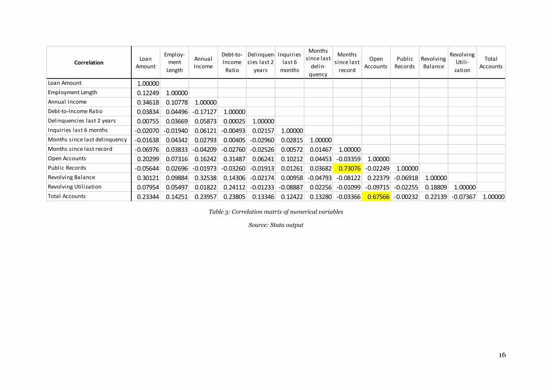
Table 3 represents the correlation matrix for the numerical variables. Variables with a high
correlation can cause some estimation problems. This will be addressed later in this paper.
Table 2: Descriptive statistics of numerical variables
Source: Stata output
16
CorrelationLoan
Amount
Employ-ment
Length
Annual Income
Debt-to-Income
Ratio
Delinquen-cies last 2
years
Inquiries last 6
months
Months since last
delin-
quency
Months since last
record
Open Accounts
Public Records
Revolving Balance
Revolving Util i-
zation
Total Accounts
Loan Amount 1.00000Employment Length 0.12249 1.00000Annual Income 0.34618 0.10778 1.00000Debt-to-Income Ratio 0.03834 0.04496 -0.17127 1.00000Delinquencies last 2 years 0.00755 0.03669 0.05873 0.00025 1.00000Inquiries last 6 months -0.02070 -0.01940 0.06121 -0.00493 0.02157 1.00000Months since last delinquency -0.01638 0.04342 0.02793 0.00405 -0.02960 0.02815 1.00000Months since last record -0.06976 0.03833 -0.04209 -0.02760 -0.02526 0.00572 0.01467 1.00000Open Accounts 0.20299 0.07316 0.16242 0.31487 0.06241 0.10212 0.04453 -0.03359 1.00000Public Records -0.05644 0.02696 -0.01973 -0.03260 -0.01913 0.01261 0.03682 0.73076 -0.02249 1.00000Revolving Balance 0.30121 0.09884 0.32538 0.14306 -0.02174 0.00958 -0.04793 -0.08122 0.22379 -0.06918 1.00000Revolving Util ization 0.07954 0.05497 0.01822 0.24112 -0.01233 -0.08887 0.02256 -0.01099 -0.09715 -0.02255 0.18809 1.00000Total Accounts 0.23344 0.14251 0.23957 0.23805 0.13346 0.12422 0.13280 -0.03366 0.67566 -0.00232 0.22139 -0.07367 1.00000
Table 3: Correlation matrix of numerical variables
Source: Stata output

17
4 Econometrical Methodology
4.1 Model selection
To use our available data and estimate a model relating the probability of default of the loan to
the borrower characteristics, we need to define the model specification and functional form
that best fits this goal and our data. According to Bolton (2009), the first step in this process is
to analyse the dependent variable. In this case, the dependent variable is the loan status at the
end of maturity. This variable can take two values, ‘Fully Paid’ or ‘Charged Off’, and is therefore
by definition a dichotomous or binary dependent variable (Wooldridge, 2002). According to
Wooldridge (2002), the most simple model to estimate and use in this situation is the linear
probability model (LPM), which is basically a multiple linear regression model where the
dependent variable is a binary variable. The model specification is defined by equation 4.1.
𝑃(𝑦 = 1|𝑥) = 𝛽0 + 𝛽1𝑥1 + ⋯ + 𝛽𝑘𝑥𝑘
In this model, the regression coefficient 𝛽𝑗 measures the change in the probability of the
occurrence of the event depicted by the dependent variable, in our case a loan default, for a
change in the predictive variable 𝑥𝑗 of 1 unit, ceteris paribus. The results of this regression can
be found in Appendix 2.
Although this model seems to fit the requirements of our case, there are some limitations that
have to be taken into account. First of all, in this model, the fitted probabilities, or the
probabilities that are a result of filling in variable values based on the observations, can be
greater than 1 and less than 0. Next to this, the partial effect of the predictor variables is
constant (Wooldridge, 2002). Finally, the error terms in the regression usually present
themselves with non-normality and heteroscedasticity, making it difficult to perform truthful
hypothesis tests based on the t-statistics the regression generates (Verbeek, 2012). These three
disadvantages of the model motivate us to explore other options.
Another binary choice model similar to the LPM is the logit model, based on the idea of
applying a transformation G on the linear relation defined by the LPM. This gives us a general
form as depicted by equation 4.2.
𝑃(𝑦 = 1|𝑥) = 𝐺(𝛽0 + 𝛽1𝑥1 + ⋯ + 𝛽𝑘𝑥𝑘)
In a logit model, this transformation G is the logistic transformation, as defined by equation
4.3. This generates a function ranging between 0 and 1 for all real numbers 𝑧 (Wooldridge,
2002).
𝐺(𝑧) = 𝑒𝑧
1 + 𝑒𝑧
(4.1)
(4.2)
(4.3)

18
If we now define 𝜋(𝑥) = 𝑃(𝑦 = 1|𝑥), and 𝑧 = (𝛽0 + 𝛽1𝑥1 + ⋯ + 𝛽𝑘𝑥𝑘), then our model
becomes:
𝜋(𝑥) = 𝑒𝛽0+ 𝛽1𝑥1+⋯+ 𝛽𝑘𝑥𝑘
1 + 𝑒𝛽0+ 𝛽1𝑥1+⋯+ 𝛽𝑘𝑥𝑘
Rearranging this to make the right hand side linear gives us equation 4.5, which is the logit
regression model we will use.
ln (𝜋(𝑥)
1 − 𝜋(𝑥)) = 𝛽0 + 𝛽1𝑥1 + ⋯ + 𝛽𝑘𝑥𝑘
To fit this model, we make use of the Maximum Likelihood Estimation, which is a method to
estimate the regression coefficients of the model by determining the combination of
coefficients or parameters that maximizes the likelihood that these estimated parameters fit
the actual population parameters, based on the observations in the sample (Wooldridge,
2002). This method defines a likelihood function that needs to be optimized iteratively, in
order to obtain the estimated parameters. In practice, we usually work with the log-likelihood
function, as it is more convenient to use (Verbeek, 2012). This log-likelihood function is
defined by equation 4.6, where 𝐹(𝑥′𝑖𝛽) = 𝑃(𝑦𝑖 = 1|𝑥𝑖; 𝛽).
log 𝐿(𝛽) = ∑ 𝑦𝑖log (𝐹(𝑥′𝑖𝛽))
𝑁
𝑖=1
+ ∑(1 − 𝑦𝑖)log (1 − 𝐹(𝑥′𝑖𝛽))
𝑁
𝑖=1
Maximizing this function gives us the estimated parameters of the model.
This model and the corresponding estimation method adequately fit the requirements of our
case. Although other models, like the tobit or probit models, would qualify as well, we decide
to use the logit model, due to the fact that this model is commonly accepted as the standard
model in credit scoring and default prediction.
4.2 Model characteristics
We now use a statistical software package, namely Stata, to estimate this model based on the
dataset we composed. Stata estimates the logit model by executing the MLE method based on
the log-likelihood function, and reports the estimated parameters, as well as some information
with respect to statistical tests. The results can be found in Table 4. The Stata command can
be found in Appendix 3.1.
Before interpreting the results, it’s important to test the characteristics of the model and its
variables.
(4.4)
(4.5)
(4.6)

19
VARIABLES Coeff Std Error
Coeff z p-value Odds Ratio
Std Error OR
Loan Amount 0.0000 0.0000 9.0224 0.000 1.0000 0.0000
Employment Length < 1 year -0.4254 0.0403 -10.5576 0.000 0.6535 0.0263
Employment Length 1 year -0.4722 0.0422 -11.1850 0.000 0.6236 0.0263
Employment Length 2 years -0.4478 0.0397 -11.2851 0.000 0.6390 0.0254
Employment Length 3 years -0.4258 0.0407 -10.4689 0.000 0.6533 0.0266
Employment Length 4 years -0.4471 0.0429 -10.4181 0.000 0.6395 0.0274
Employment Length 5 years -0.4390 0.0412 -10.6594 0.000 0.6447 0.0266
Employment Length 6 years -0.3596 0.0426 -8.4440 0.000 0.6980 0.0297
Employment Length 7 years -0.3590 0.0438 -8.2029 0.000 0.6984 0.0306
Employment Length 8 years -0.3817 0.0465 -8.2153 0.000 0.6827 0.0317
Employment Length 9 years -0.4058 0.0501 -8.0948 0.000 0.6665 0.0334
Employment Length 10+ years -0.3955 0.0342 -11.5521 0.000 0.6734 0.0231
Dummy Home Mortgage -0.1521 0.0274 -5.5406 0.000 0.8589 0.0236
Dummy Home Rent 0.1052 0.0268 3.9247 0.000 1.1109 0.0298
Annual Income 0.0000 0.0000 -21.0859 0.000 1.0000 0.0000
Debt-to-Income Ratio 0.0128 0.0011 11.3438 0.000 1.0129 0.0011
Delinquencies 2 years 0.0557 0.0135 4.1443 0.000 1.0573 0.0142
Earliest Credit Line 0.0000 0.0000 6.9047 0.000 1.0000 0.0000
Inquiries last 6 months 0.2111 0.0059 36.0733 0.000 1.2350 0.0072
Months since last delinquency -0.0005 0.0006 -0.7065 0.480 0.9995 0.0006
Dummy Delinquencies 0.0999 0.0316 3.1591 0.002 1.1051 0.0350
Months since last record 0.0003 0.0010 0.2806 0.779 1.0003 0.0010
Dummy Public Records 0.0844 0.1043 0.8085 0.419 1.0880 0.1135
Open Accounts 0.0248 0.0023 10.8474 0.000 1.0251 0.0023
Public Records 0.0049 0.0326 0.1493 0.881 1.0049 0.0328
Revolving Balance 0.0000 0.0000 -0.5469 0.584 1.0000 0.0000
Revolving Utilization 0.8345 0.0339 24.6008 0.000 2.3037 0.0781
Total Accounts -0.0115 0.0010 -11.0940 0.000 0.9886 0.0010
Listing Status 0.0768 0.0197 3.9060 0.000 1.0798 0.0212
Constant -2.5773 0.0682 -37.7908 0.000 0.0760 0.0052
4.2.1 Goodness of Fit
To estimate the goodness of fit of our model, or how well the model fits the observed data
(Verbeek, 2012), we analyse the pseudo R-squared statistic of the model, which is a statistic
ranging from 0 to 1. There are several ways to calculate the pseudo R-squared of a logit model,
but there is no agreement on which one of them is the preferred one to use.
Table 4: Regression results initial model - coefficients and odds ratios
Source: Stata output

20
The pseudo R-squared of our model, reported by Stata, is 0.0301. Although a single pseudo R-
squared statistic of a logit model can’t be accurately interpreted on its own, this value clearly
indicates that our model performs poorly in its ability to fit the data. This could be the result
of the possibility that the model is incomplete, and that we require other variables to more
accurately predict the probability of default. Unfortunately, we are restricted by our data set,
and therefore, no other variables are available.
However, in logit models, the goodness of fit of the model is relatively unimportant compared
to the statistical and economic significance of the model and its predictor variables
(Wooldridge, 2002). We therefore leave these findings out of account in the remainder of this
analysis, and focus on the estimated regression coefficients and their interpretation.
4.2.2 Model significance
Assessing the significance of a logit model essentially comes down to comparing the full model
to the model where the only predictor variable is a constant, and determining whether the log-
likelihood of the full model is statistically significantly greater than the log-likelihood of the
restricted model. According to the likelihood ratio test, as described by Wooldridge (2002), a
likelihood ratio (LR) test statistic is calculated, as illustrated by equation 4.7.
𝐿𝑅 = 2(ℒ𝑓𝑢𝑙𝑙 − ℒ𝑟𝑒𝑠𝑡𝑟𝑖𝑐𝑡𝑒𝑑)
This test statistic has a chi-square distribution of which the number of degrees of freedom is
equal to the difference between the number of predictor variables in the full model and the
number of predictor variables in the restricted model.
Calculating the LR test statistic of our model gives us a value of 3990.604. The critical chi-
square value with a significance level of 1% and 29 degrees of freedom is approximately 49.59.
The test statistic exceeds this value, and we can therefore conclude that the model is
statistically significant on a significance level of 1%.
4.2.3 Significance of variables
Assessing the significance of the variables in our model can be done by testing whether the
regression coefficient corresponding to each predictor variable is statistically significantly
different from 0. The easiest way to do this is by looking at the p-values of the coefficients. A
p-value represents the strongest significance level on which the null hypothesis of the
coefficient being statistically not significantly different from 0 can be rejected (Wooldridge,
2002). In other words, it represents the strongest significance level on which the coefficient is
significantly different from 0.
Based on the model output in Table 4, we can observe that most of the coefficients are
statistically significantly different from 0, with p-values close to or equal to zero. There are 5
(4.7)

21
coefficients, however, of which the p-value indicates that they are not statistically significantly
different from 0. These coefficients are the ones corresponding to the variables ‘months since
last delinquency’, ‘months since last record’, ‘dummy public records’, ‘public records’ and
‘revolving balance’. The economic implications of these findings will be discussed in a later
section, where the results of this research are analysed.
4.2.4 Coefficient interpretation
The interpretation of the regression coefficients of a logistic regression is rather different from
that of an OLS regression. As can be derived from the model depicted by equation 4.5, a
regression coefficient represents the increase in the logarithmic odds of the occurrence of the
event coded in the dependent variable, in our case a loan default, for an increase of the
predictor variable of 1 unit, all other variables remaining constant (Verbeek, 2012). This
relation is rather difficult to interpret, and we therefore generate odds ratios for each predictor
variable. To do so, we simply raise the mathematical constant e to the power of the coefficient
corresponding to each variable, as illustrated by equation 4.8. This can be done in Stata by
using the ‘logistic’ command, as illustrated in Appendix 3.2. The results have been added to
Table 4.
𝑂𝑅𝑖 = 𝑒𝛽𝑖
In our model, the odds ratio corresponding to a certain predictor variable is the ratio of the
odds that a loan will default to the odds that it will not, for a one-unit increase in the value of
the predictor variable. In other words, it represents the multiplicator that defines the change
in the odds of a loan default for a one-unit increase in the value of the predictor variable.
An odds ratio typically ranges from zero to positive infinity. A value lower than 1 represents a
decrease in the odds of the probability of default, and therefore corresponds to a negative
relation between the dependent variable and the predictor variable. An odds ratio of exactly 1
implies no relation between the dependent variable and the predictor variable. Note that an
odds ratio of 1 corresponds to a regression coefficient of 0, or by definition a statistically
insignificant regression coefficient An odds ratio greater than 1 corresponds to a positive
relation between the dependent variable and the predictor variable.
The odds ratios corresponding to each predictor variable, and their implications in our model,
will be discussed in a following section.
(4.8)

22
5 Specification Adjustments
Before we can correctly interpret the results of our model, some adjustments need to be made
to our initial specification. These adjustments, the reason behind them, and their implications
for our model are discussed in this section.
5.1 Employment length
As previously mentioned, the variable ‘employment length’ has been recoded into 11 dummy
variables, primarily to test for multiple relations between this variable and the probability of
default. The regression coefficients of these dummy variables, including a linear trendline, are
displayed in Figure 3.
At first sight, there seems to be no clear positive or negative relation between the increase or
decrease of employment length of the borrower and his probability of default. The trendline
doesn’t give a definitive answer as well, showing only a marginally positive2 relation. This
initial finding corresponds with the findings in the study conducted by Serrano-Cinca,
Gutiérrez-Nieto & López-Palacios (2015), where no significant relation was found as well. We
can therefore conclude that employment length doesn’t have a significant impact on the
probability of default of the borrower.
2 This positive relation is counter-intuitive, because it indicates that the probability of default is higher when the borrower is employed for a longer time.
Figure 3: Regression coefficients employment length, including linear trendline
Source: Stata output, own calculations
-0.5
-0.45
-0.4
-0.35
-0.3
-0.25
-0.2
-0.15
-0.1
-0.05
0
<1y 1y 2y 3y 4y 5y 6y 7y 8y 9y 10+y
Co
effi
cien
t
Employment Length
Regression coefficients Employment Length

23
However, due to the fact that every regression coefficient is statistically significantly different
from zero, the employment status of the borrower does seem to have an impact. The data points
towards the possibility that a borrower with a job has a significantly lower probability of default
than an unemployed borrower. We can test this by replacing the 11 dummy variables in our
model with a single new dummy variable, ‘employment’, representing whether or not the
borrower is employed. A value of 1 indicates employment, a value of 0 represents
unemployment.
Comparing the new model with the initial model by the use of the LR test will teach us if there
is a statistical difference between these two models. No statistical difference points towards no
loss of information and predictive power of the model, and therefore a valid replacement of
variables.
The LR test statistic, calculated according to equation 4.7, equals 17.82. The critical chi-square
value with a significance level of 1% and 10 degrees of freedom amounts to approximately
23.21. The test statistic doesn’t exceed the critical value, which means the null hypothesis of no
statistical difference between the models can’t be rejected. Our replacement of variables is
therefore valid, and the adjusted specification can be used. The results of this regression can
be found in Table 6, in the column of Model 1.
5.2 Open Accounts & Total Accounts
As can be seen in Table 3, we found a relatively high correlation (0.67566) between the
variables ‘open accounts’ and ‘total accounts’. This high correlation could result in a biased
estimation of the corresponding regression coefficients. We therefore execute the regression
twice, where each of these two variables will be integrated individually. This has given rise to
the results that can be found in Table 6, labelled as Model 2 and Model 3.
Based on these results, we can conclude the following. Both variables remain statistically
significant, and their relation with the dependent variable remains the same as in the initial
model. Only the actual value of the regression coefficients slightly differs from those of the
initial specification, as can be expected. We therefore decide to keep both variables in the
model.
5.3 Public records & Months since last record
Table 3 shows us that the variables ‘public records’ and ‘months since last record’ are highly
correlated as well, with a correlation of 0.73076. We therefore again execute two regressions,
each containing one of the highly correlated variables. The results of these regressions can be
found in Table 6, in the column of Model 4 and Model 5.

24
These results show us that the variable ‘months since last record’ and its corresponding dummy
variable remain statistically not significant, whereas the variable ‘public records’ becomes
significant when integrated separately into our model. We therefore decide to only keep the
significant variable ‘public records’ in our model.
The regression coefficients of each of the models used in this section are summarised in Table
6. Model 1 is the full model, where the dummy variables for employment length have been
replaced with a single dummy variable representing the employment status of the borrower.
This model serves as the basis for the following adaptions. In Model 2, the variable ‘total
accounts’ has been left out, and in Model 3, the same has been done for the variable ‘open
accounts’. In Model 4, the variables ‘months since last record’ and ‘dummy public records’ have
been omitted, and in Model 5, this is the case for the variable ‘public records’.
In conclusion, the final model that will serve as the base for our analysis is the model as
presented in Table 5, where the dummy variable ‘employment’ has been introduced as a
replacement for the dummies of the variable ‘employment length’. Next to this, the variables
‘months since last record’ and ‘dummy public records’ have been omitted due to their high
correlation with ‘public records’ and their statistical insignificance, and the variables ‘months
since last delinquency’ and ‘revolving balance’ have been omitted due to their statistical
insignificance.
VARIABLES Coeff Std Dev z p-value Odds Ratio
Std Dev OR
Loan Amount 0.0000110 1.21e-6 9.0713 0.000 1.0000110 1.21e-6
Employment -0.4142 0.0323 -12.8412 0.000 0.6609 0.0213
Dummy Home Mortgage -0.1475 0.0274 -5.3791 0.000 0.8629 0.0237
Dummy Home Rent 0.1011 0.0267 3.7811 0.000 1.1064 0.0296
Annual Income -0.0000062 2.8e-7 -22.1264 0.000 0.9999938 2.8e-7
Debt-to-Income Ratio 0.0128 0.0011 11.4887 0.000 1.0129 0.0011
Delinquencies 2 years 0.0602 0.0111 5.4421 0.000 1.0620 0.0117
Earliest Credit Line 0.0000216 3.22e-6 6.7201 0.000 1.0000216 3.22e-6
Inquiries last 6 months 0.2104 0.0058 36.0289 0.000 1.2342 0.0072
Dummy Delinquencies 0.0827 0.0164 5.0349 0.000 1.0862 0.0178
Open accounts 0.0243 0.0023 10.7526 0.000 1.0246 0.0023
Public records 0.0622 0.0170 3.6682 0.000 1.0642 0.0180
Revolving utilization 0.8330 0.0332 25.0895 0.000 2.3002 0.0764
Total Accounts -0.0114 0.0010 -11.0754 0.000 0.9887 0.0010
Listing Status 0.0737 0.0196 3.7541 0.000 1.0765 0.0211
Constant -2.5489 0.0675 -37.7650 0.000 0.0782 0.0053
Table 5: Regression results Final Model
Source: Stata output

25
(1) (2) (3) (4) (5)
VARIABLES Model 1 Model 2 Model 3 Model 4 Model 5
Loan Amount 1.12e-05*** 1.07e-05*** 1.15e-05*** 1.11e-05*** 1.12e-05***
(1.22e-06) (1.22e-06) (1.22e-06) (1.22e-06) (1.22e-06)
Employment -0.411*** -0.411*** -0.398*** -0.414*** -0.411***
(0.0323) (0.0323) (0.0322) (0.0323) (0.0323)
Dummy Home Mortgage -0.149*** -0.168*** -0.151*** -0.147*** -0.149***
(0.0274) (0.0274) (0.0274) (0.0274) (0.0274)
Dummy Home Rent 0.100*** 0.105*** 0.104*** 0.101*** 0.100***
(0.0268) (0.0267) (0.0267) (0.0268) (0.0268)
Annual Income -6.13e-06*** -6.64e-06*** -5.99e-06*** -6.14e-06*** -6.13e-06***
(2.91e-07) (2.90e-07) (2.89e-07) (2.91e-07) (2.91e-07)
Debt-to-Income Ratio 0.0130*** 0.0113*** 0.0156*** 0.0129*** 0.0130***
(0.00113) (0.00112) (0.00110) (0.00113) (0.00113)
Delinquencies 2 years 0.0553*** 0.0509*** 0.0561*** 0.0551*** 0.0553***
(0.0134) (0.0134) (0.0134) (0.0134) (0.0134)
Earliest Credit Line 2.18e-05*** 2.98e-05*** 2.54e-05*** 2.13e-05*** 2.18e-05***
(3.27e-06) (3.22e-06) (3.26e-06) (3.26e-06) (3.27e-06)
Inquiries last 6 months 0.210*** 0.206*** 0.211*** 0.210*** 0.210***
(0.00584) (0.00582) (0.00583) (0.00584) (0.00584)
Months since last delinquency -0.000431 -0.000379 -0.000336 -0.000406 -0.000431
(0.000640) (0.000641) (0.000640) (0.000640) (0.000640)
Dummy Delinquencies 0.100*** 0.0702** 0.0876*** 0.0983*** 0.100***
(0.0316) (0.0315) (0.0316) (0.0316) (0.0316)
Months since last record 0.000356 0.00142 0.000881 0.000317
(0.000975) (0.000967) (0.000972) (0.000945)
Dummy public records 0.0816 -0.0245 0.0289 0.0909
(0.104) (0.101) (0.102) (0.0867)
Open accounts 0.0245*** 0.00955*** 0.0245*** 0.0245***
(0.00228) (0.00184) (0.00228) (0.00228)
Public records 0.00527 0.0142 0.0101 0.0617***
(0.0324) (0.0292) (0.0308) (0.0170) Revolving balance -3.15e-07 -2.77e-07 2.98e-07 -4.16e-07 -3.16e-07
(5.87e-07) (5.92e-07) (5.50e-07) (5.91e-07) (5.87e-07)
Revolving utilization 0.838*** 0.854*** 0.773*** 0.838*** 0.838***
(0.0339) (0.0339) (0.0331) (0.0339) (0.0339)
Total Accounts -0.0114*** -0.00494*** -0.0114*** -0.0114***
(0.00103) (0.000827) (0.00103) (0.00103)
Listing Status 0.0753*** 0.0769*** 0.0719*** 0.0739*** 0.0753***
(0.0196) (0.0196) (0.0196) (0.0196) (0.0196)
Constant -2.568*** -2.708*** -2.545*** -2.548*** -2.568***
(0.0678) (0.0670) (0.0679) (0.0675) (0.0678)
Observations 175,037 175,037 175,037 175,037 175,037
Standard errors in parentheses *** p<0.01, ** p<0.05, * p<0.1
Table 6: Regression coefficients for different specifications
Source: Stata output

26
6 Empirical Results
This section analyses the results of the regression by interpreting the regression coefficients
and odds ratios corresponding to the variables incorporated into our model. These results can
be found in Table 5. We compare these findings with those of similar studies and the current
literature on credit scoring in P2P-Lending, and consequently draw conclusions.
As previously described, the model defines a relation between the probability of default of a
loan issued by Lending Club on the one hand, and a set of predictor variables gathered by
Lending Club during the loan application process on the other hand. Therefore, when we talk
about the probability of default, we are referring to the probability of the borrower defaulting
on his loan at Lending Club.
6.1 Non-significant variables
We first take a look at the variables for which we previously found that their regression
coefficients are statistically not significantly different from zero. As mentioned above, these
variables are ‘months since last delinquency’, ‘months since last record’, ‘dummy months since
last record’ and ‘revolving balance’. Note that the variable ‘public records’ has become
statistically significant after the removal of the highly correlated variable ‘months since last
record’ from our model.
Delinquencies
The coefficient of the variable ‘months since last delinquency’ is, according to our model,
statistically not significantly different from zero. This implies that how long ago a borrower
had his last delinquency doesn’t impact his probability of defaulting on his loan at Lending
Club. If we analyse ‘dummy months since last delinquency’, the corresponding dummy variable
we created to capture the effect of the difference between ever having had a delinquency or not,
we can conclude the following. The dummy variable is statistically significantly different from
zero, which implies that whether or not the borrower ever had a delinquency, does impact his
probability of default. The odds ratio of this dummy variable amounts to 1.0862. This points
towards a positive relation between the borrower having a delinquency recorded on his credit
file and the probability of default, and indicates that the odds of default are approximately
8.62% higher if the borrower ever had a delinquency, compared to never having had a
delinquency.
The variable ‘delinquencies 2 years’, representing the amount of delinquencies in the past two
years, has a significant coefficient as well. According to the odds ratio corresponding to this
variable, which is equal to 1.0620, each additional delinquency in the past two years increases
the odds of a default on the loan of the borrower with approximately 6.20%.
27
These findings are in line with what has been found in previous studies. As can be expected,
borrowers who have had delinquencies in the past, are more likely to miss payments or default
on their loan in the future (Nefer, 2010). The Fair Isaac Corporation, developer of the FICO-
score, states that historical payment behaviour determines 35% of a borrower’s credit score
(Fair Isaac Corporation, 2017). Next to this, Serrano-Cinca, Gutiérrez-Nieto and López-
Palacios (2015) also found a positive relation between the amount of delinquencies and the
probability of default, and no statistical relation between the number of months since the
borrower’s last delinquency and his probability of default.
Public records
The next set of variables we will discuss are the variables relating to public records in the credit
file of the borrower. These variables are ‘public records’, ‘months since last record’ and ‘dummy
records’. As previously mentioned, the variables ‘months since last record’ and ‘dummy
records’ appear to have a regression coefficient that is statistically not significantly different
from zero. This implies that the amount of months since the last time a public record was
recorded in the credit file of the borrower has no impact on his probability of default.
The variable ‘public records’ however, does have a regression coefficient that is statistically
significantly different from zero. The amount of public records in the credit file of the borrower
seems to have an impact on the probability of default of the borrower, and, as can be expected,
the relation is positive. With a regression coefficient of approximately 0.0622 and a
corresponding odds ratio of approximately 1.0642, we can state that, according to our model,
each additional public record in the credit file of the borrower increases the odds of defaulting
by approximately 6.42%.
This is more or less in line with what has been found in similar studies. According to Credit
Karma (2012), public records on the credit report of a borrower have a significant negative
impact on his credit score, and subsequently his probability of default. The study conducted by
Serrano-Cinca et al. (2015) shows that the number of public records on the credit file of the
borrower is positively correlated with his probability of default.
This positive relation can easily be explained from an economic point of view. Public records
are the result of serious financial delinquencies, such as bankruptcies or tax liens. In case of a
tax lien, for example, the borrower owes a substantial amount of tax money to the state, who
has a legal claim on the assets of the noncompliant taxpayer. The consequences of these
delinquencies can therefore have a significant impact on the financial status of the borrower.
This places the borrower in a vulnerable position with respect to future financial obligations,
and he therefore has an increased change of not being able to fulfil these obligations in the
future.

28
Revolving balance
The final variable of which the regression coefficient is statistically not significantly different
from zero is the variable ‘revolving balance’. This implies that the total credit revolving balance
over the lifetime of the borrower has no impact on his probability of defaulting on future loans.
This finding is in line with what has been found in the study conducted by Emekter, Tu,
Jirasakuldechc, & Lu (2015). In most of the studies, however, the focus lies on the revolving
line utilization, or the average amount of credit used relative to the total available credit. This
variable is integrated into our model as well, and will be analysed in the following section.
6.2 Significant variables
We now further analyse the variables for which the regression coefficient is statistically
significantly different from zero, and consequently seem to have an impact on the probability
of default of the borrower.
Loan amount
The regression coefficient on the variable loan amount is in our model equal to 0.000011. To
make the interpretation of this coefficient and its corresponding odds ratio more meaningful,
we multiply it by 100, giving us a coefficient of approximately 0.0011. The corresponding odds
ratio is found by raising e to the power of this coefficient, and results in an odd ratio of
approximately 1.001101. Interpreting this odds ratio explains us that according to our model,
the odds of defaulting on the loan increase by approximately 0.11% for every increase in the
loan amount of 100 units (or 100 dollar).
At first sight, this seems logical. The higher the amount the borrower wants to borrow, the
higher his monthly installment, and, ceteris paribus, the bigger the chance the borrower won’t
be able to fulfil these payment obligations. However, the study conducted by Serrano-Cinca et
al. (2015) seems to find no relation between the loan amount and the probability of default.
Similarly, a study by Kočenda and Vojtek (2009), where three models were tested, found that
in two of their models, the loan amount was negatively correlated with the probability of
default, whereas in the third model, a positive relation was found. We can therefore conclude
that, based on these findings, there is generally no clear relation between the loan amount and
the probability of default.
Employment
As previously stated, the length of employment doesn’t seem to have an impact on the
probability of default of the borrower. However, according to our final model, the employment
status does have a statistically significant impact on the probability of default. With an odds
ratio of approximately 0.6609, we can state that for a borrower who has a job, the odds of

29
defaulting are, ceteris paribus, approximately 23.91% lower compared to a borrower without
a job.
From an economic point of view, this finding makes perfect sense. Being employed generally
means having a steady income, which creates certainty for the future. This certainty is very
important for investors, as it indicates that the borrower will remain creditworthy during the
maturity of the loan, and will consequently continue to be able to fulfil his financial obligations.
The length of employment plays a minor role in this certainty. One could state that the longer
the borrower is employed, the more certain he is of keeping his job. This statement, however,
isn’t supported by the data, and we therefore conclude that the employment status of the
borrower plays by far the most important role compared to the employment length.
Home ownership
For the categorical variable ‘home ownership’, the dummy variables ‘dummy house mortgage’
and ‘dummy house rent’ have been created. The first dummy captures the difference in
probability of default between owning a house and having a mortgage on your house, and the
second dummy does this for the difference between owning a house and renting one. Analysing
the odds ratios of these dummies, which are 0.8629 and 1.1064 respectively, allows us to
conclude the following. The odds of defaulting decrease by approximately 13.71% when the
borrower has a mortgage on his house compared to owning a house, ceteris paribus. In the
other case, for a borrower renting his house compared to a borrower owning a house, the odds
of defaulting are approximately 10.64% higher, ceteris paribus. All of this indicates that
borrowers renting a house are more likely to default compared to borrowers owning a house,
whereas borrowers having a mortgage on their home are less likely to default. These findings
are in line with those of Serrano-Cinca et al. (2015).
Annual income
Concerning the variable ‘annual income’, we intuitively expect a negative relation between the
probability of default and the amount of annual income of the borrower. Indeed, the regression
coefficient is negative and the odds ratio is lower than 1. Multiplying the regression coefficient
by 1000 and calculating the corresponding odds ratio, results in an odds ratio of approximately
0.9938. This indicates that for every additional 1000 dollar of annual income, the odds of
defaulting on the loan decrease with approximately 0.62%. Other studies come to the same
conclusion concerning this negative relation.
Debt-to-income ratio
The next variable we analyse is the ‘debt-to-income ratio’ variable. This variable has a
significant regression coefficient and an odds ratio of 1.0128. As can be expected, this implies
a positive relation between the debt-to-income ratio of a borrower and his probability of

30
default. More specifically, the odds ratio indicates that for every increase in the debt-to-income
ratio of one unit, the odds of defaulting on the loan increase with approximately 1.28%. This
positive relation is also found in the studies conducted by Serrano-Cinca et al. (2015),
Carmichael (2014), Ponela & Regner (2016) and Emekter et al. (2015). Intuitively, this relation
makes sense as well. The more debt a borrower has relative to his income, the harder it is for
him to fulfil all of his financial obligations, and the higher his probability of defaulting on these
obligations. This statement is also supported by what can be seen in Figure 1 and Figure 2,
where the main determinants of the FICO-score and VantageScore 3.0 are illustrated. Both
scoring models allocate a substantial weight to the amount of debt of the borrower.
Earliest credit line
The variable ‘earliest credit line’ represents the date on which the borrower has opened his first
credit line. Each unit of this variable represents one day. For interpretation purposes, we
therefore multiply the regression coefficient of 0.000022 with 365, and calculate the
corresponding odds ratio. This odds ratio equals approximately 1.0079, indicating that the
more recent a borrower opened his first credit line, the higher his probability of default. More
precisely, according to this odds ratio, a borrower who has opened his first credit line one year
later than another borrower, has, ceteris paribus, increased odds of defaulting of
approximately 0.79%. This finding is in line with what has been found by Serrano-Cinca et al.
(2015) Polena & Regner (2016) and Carmichael (2014).
Inquiries in the last 6 months
The variable ‘inquiries in the last 6 months’, representing the amount of hard inquiries on the
credit report of the borrower during the last 6 months, has a significant, positive regression
coefficient, and a corresponding odds ratio of approximately 1.2342. This indicates that for
each additional hard inquiry on the credit file of the borrower during the last 6 months, the
odds of defaulting increase with approximately 23.42%. The study conducted by Serrano-Cinca
et al. (2015) confirms this positive relation.
From an economic point of view, this could be explained as follows. A lot of recent inquiries
indicates that the borrower has applied for a loan several times during the last six months. This
could mean that he has either engaged in a lot of loan commitments, or that he has been
rejected several times during a loan application. Both situation indicate an unhealthy financial
situation. On the one hand, a lot of loan commitments result in a lot of payment obligations,
and consequently a higher chance of not fulfilling these obligations. A lot of loan rejections on
the other hand clearly indicate that there is little believe in the creditworthiness of the
borrower. We can therefore conclude that from an economic point of view, a high amount of
inquiries on your credit report corresponds to a higher probability of default.

31
Open accounts
The number of open accounts in the credit file of the borrower has, according to our model, a
significant impact on the probability of default as well. With an odds ratio of approximately
1.0246, we can state that for each additional open account on the credit file of the borrower,
his odds of defaulting increase by approximately 2.46%. However, this finding is not supported
by the similar studies. The study conducted by Serrano-Cinca et al. (2015) finds a significant
negative relation, whereas Polena & Regner (2016) and Emekter et al. (2015) find no significant
relation between the number of open accounts and the probability of default of the borrower.
Reasons for these discrepancies could be the use of different data sets, or the possibility that
previously found relations have changed due to learning effects in the financial market.
Nevertheless, we conclude that we can’t make decisive conclusions on the relation between the
number of open accounts in the credit file of the borrower and his probability of default.
Revolving utilization
As previously mentioned, similar studies have shown that the variable ‘revolving utilization’
has a quite significant impact on the probability of default of a borrower. This statement is
supported by studies conducted by Serrano-Cinca et al. (2015), Emekter et al. (2015) and
Carmichael (2014). With an odds ratio of approximately 2.3, our model tells us that for every
increase in the revolving utilization of the borrower of 1 unit (or 100 percentage points), the
odds of defaulting increase by approximately 130%. Recalculating the odds ratio for an increase
of 10 percentage points gives us an odds ratio of approximately 1.087, indicating that an
increase in the revolving utilization of 10 percentage points results in an increase in the odds
of defaulting of approximately 8.7%. If we again take a look at Figure 2, we can see that the
amount of credit used relative to the available credit plays an important role in the calculation
of the VantageScore 3.0. Indeed, borrowers who use a substantial amount of their available
credit might have more problems repaying that credit, resulting in a higher probability of
defaulting on these and other financial obligations.
Total accounts
According to our model, the total number of accounts, as currently reported by the borrowers
credit file, has a significant impact on his probability of default as well. However, as opposed
to the variable ‘open accounts’, this variable has a negative relation with the probability of
default. The odds ratio of 0.9887 indicates that for every additional account recorded in the
credit file of the borrower, his odds of defaulting decrease by approximately 1.13%. Here as
well, this statement is not in line with what other studies report. For example, Emekter et al.
(2015) find no significant relation. These discrepancies could again be the result of the use of
different data set or learning effects in the financial market, but we are forced to conclude that,
based on this analysis, no clear relation can be determined.

32
Listing status
The last variable discussed in this paper is the dummy variable ‘listing status’. As previously
described, this variable takes a value of 0 for an initial listing status of ‘whole’, and a value of 1
for an initial listing status of ‘fractional’. The odds ratio corresponding to this dummy variable
is 1.0765, which indicates that the odds of defaulting are, ceteris paribus, approximately 7.65%
higher for a ‘fractional’ loan compared to a ‘whole’ loan.
The reason behind this result is difficult to determine, mainly due to the fact that at first sight,
the listing status of the loan has nothing to do with the creditworthiness of the borrower. Other
studies haven’t incorporated this variable in their research either. Therefore, it is likely that
this finding is coincidental, and the listing status has in reality no real economic impact on the
probability of default of the borrower, but merely a statistical correlation with it. Additional
studies where this variable is included could confirm or deny this statement.

33
7 Conclusion
The aim of this dissertation was to define the main determinants of loan default in the P2P-
Lending market, by developing a statistical model that relates the probability of default of a
borrower to several borrower characteristics gathered during the loan application process. For
this analysis, we used a data set provided by Lending Club, the largest P2P-Lending platform
in the US. Based on current literature on credit scoring, in combination with the available data,
we defined several model specifications to correctly determine the significance and impact of
each of the variables under consideration. This has led to a final model, that served as the base
for the analysis of the results. Based on these results, we can conclude the following.
First of all, we concluded that delinquencies and public records registered in the credit file of
the borrower raise his probability of default, and the more delinquencies or public records, the
higher this probability of default. However, the time since the last registered delinquency or
public record seems to have no impact of the default probability.
Next to this, we found that the amount of revolving balance of the borrower has no real impact
on the probability of default as well. The utilization rate of this revolving balance, however,
does have a significant impact. The higher this utilization rate, the higher the probability of
default of the borrower.
With respect to employment, we found that the employment length has no significant impact
on the probability of default, but the employment status does. A borrower with a job has a
substantially lower probability of default compared to a borrower without a job. The annual
income of the borrower plays a significant role as well. As can be expected, the higher the
income, the lower the probability of default.
Continuing with the solvency of the borrower, we can state the following. The ratio of current
debt to total income has proven to be a powerful predictor of future loan default, with a high
debt-to-income ratio corresponding to a high probability of default. The loan amount,
however, has a more unclear relation with the default probability. Our study found a positive
relation, but this is contradicted by other studies, where negative or insignificant relations are
found. We therefore refrain from drawing decisive conclusions with respect to the loan
amount.
The home ownership has a significant impact as well. According to our analysis, a borrower
who has a mortgage on his house has the lowest probability of default, followed by a borrower
who is the owner of his home. A borrower who rents his house has the highest probability of
defaulting on his loan.
Finally, we found that the variables relating to the credit record of the borrower yield some
valuable information as well. First of all, we can state that the more hard inquiries that have
been made on the credit file of the borrower, the higher his probability of default is. Secondly,

34
we found that the longer ago a borrower has opened his first credit line, the lower his
probability of default. The impact of the number of accounts in the credit file of the borrower
is less clear. Based on our analysis, we found a positive relation for the number of open
accounts, and a negative relation with the probability of default for the number of total
accounts. This opposite relation in itself is rather counterintuitive, and similar studies
contradict these findings as well. We therefore again decide to refrain from drawing
conclusions with respect to the accounts registered in the credit file of the borrower.
8 Further Research
The analysis in this paper, and the corresponding results, have been compared with the
findings from several similar studies in order to draw meaningful conclusions. However, it
needs to be noted that this study is insufficient in drawing a truthful image of the determinants
of loan default in the P2P-Lending market. This is due to several shortcomings. First of all, this
study is focused on data from Lending Club, who is only one of the major players in the P2P-
Lending market. Next to this, we focused only on loans with a maturity of 36 months. These
two points show that there is ample opportunity to take further steps in this field of research.
A first step could be to conduct the same analysis with a data set containing the Lending Club
loans with a maturity of 60 months, and comparing those results with the ones found in this
paper. Next to this, similar studies could be conducted with data from other P2P-Lending
platforms, again comparing both results.

I
References
Bajpai, P. (2015). The 7 Best Peer-To-Peer Lending Websites (LC). Investopedia.
Berger, S. C., & Gleisner, F. (2009). Emergence of Financial Intermediaries in. BuR - Business
Research, 39-65.
Credit Karma. (2012, January 12). Public Records on Your Credit Report. Retrieved from
Credit Karma: https://www.creditkarma.com/article/public-records-on-credit-report
Dujeux, F. (2017, February 15). Interview with Frédéric Dujeux, Co-Founder of Mozzeno.
(Wiseclerk, Interviewer)
Emekter, R., Tu, Y., Jirasakuldechc, B., & Lu, M. (2015). Evaluating credit risk and loan.
Applied Economics, 47(1), 54-70.
Fair Isaac Corporation. (2017). Learn About The FICO® Score and its Long History. Retrieved
from Fico: http://www.fico.com/25years/
Fair Isaac Corporation. (2017). Why are my FICO® Scores different for the 3 credit bureaus?
Retrieved from myFICO: http://www.myfico.com/credit-education/questions/why-
are-my-credit-scores-different-for-3-credit-bureaus/
Finger, R. (2013, May 30). Banks Are Not Lending Like They Should, And With Good Reason.
Retrieved from Forbes:
http://www.forbes.com/sites/richardfinger/2013/05/30/banks-are-not-lending-like-
they-should-and-with-good-reason/#348fd0fe44b1
Fintechnews Singapore. (2016, June 29). Asia’s Top 7 Peer-to-Peer Lending Platforms.
Retrieved from Fintechnews: http://fintechnews.sg/3518/crowdfunding/asias-top-7-
peer-peer-lending-platforms/
Fintechnews Switzerland. (2016, July 1). Europe’s Top 11 Peer-to-Peer Lending Platforms.
Retrieved from Fintech News: http://fintechnews.ch/p2plending/europes-top-11-
peer-to-peer-lending-platforms/4960/
Gurney, I. (2017). Companies. Retrieved from p2pmoney:
http://www.p2pmoney.co.uk/companies.htm
Hörkkö, M. (2010). The Determinants of Default in Consumer Credit Market. Aalto University
School of Economics.

II
Hulme, M. K., & Wright, C. (2006). Internet Based Social Lending: Past, Present and Future.
Social Futures Observatory.
Investopedia. (n.d.). Adverse Selection. Retrieved from Investopedia:
http://www.investopedia.com/terms/a/adverseselection.asp
Investopedia. (n.d.). Asymmetric Information. Retrieved from Investopedia:
http://www.investopedia.com/terms/a/asymmetricinformation.asp
Investopedia. (n.d.). Credit Scoring. Retrieved from Investopedia:
http://www.investopedia.com/terms/c/credit_scoring.asp
Investopedia. (n.d.). Moral Hazard. Retrieved from Investopedia:
http://www.investopedia.com/terms/m/moralhazard.asp
Investopedia. (n.d.). Peer-To-Peer Lending (P2P). Retrieved from Investopedia:
http://www.investopedia.com/terms/p/peer-to-peer-lending.asp
Investopedia. (n.d.). Revolving Credit. Retrieved from Investopedia:
http://www.investopedia.com/terms/r/revolvingcredit.asp
Investopedia. (n.d.). Unsecured Loan. Retrieved from Investopedia:
http://www.investopedia.com/terms/u/unsecuredloan.asp
Irby, L. (2016, November 10). Public Records and Your Credit Report. Retrieved from
thebalance: https://www.thebalance.com/public-records-and-your-credit-report-
960740
Irby, L. (2016, September 1). What is a Hard Inquiry? Retrieved from thebalance:
https://www.thebalance.com/what-is-a-hard-inquiry-960549
Kočenda, E., & Bojtek, M. (2009). Default Predictors and Credit Scoring Models. CESifo.
LendingClub Corporation. (2017). Lending Club Statistics. Retrieved from Lending Club:
https://www.lendingclub.com/info/statistics.action
Lin, M., Prabhala, N. R., & Viswanathan, S. (2013). Judging Borrowers by the Company They
Keep: Friendship. Management Science, 17-35.
Mateeschu, A. (2015). Peer-to-Peer Lending. Data&Society, 1-23.
Nefer, B. (2010, November 12). What Does Delinquency on a Credit Report Mean? Retrieved
from Sapling: https://www.sapling.com/7491164/delinquency-credit-report-mean

III
Nickolas, S. (2015, April 24). What is the difference between moral hazard and adverse
selection? Retrieved from Investopedia:
http://www.investopedia.com/ask/answers/042415/what-difference-between-moral-
hazard-and-adverse-selection.asp
Polena, M., & Regner, T. (2016). Determinants of borrowers' default in P2P lending. Jena
Economic Research Papers, No. 2016-023.
Prosper Marketplace, Inc. (2017). About us. Retrieved from Prosper:
https://www.prosper.com/plp/about/
Renton, P. (2012). The Lending Club Story: How the world's largest peer to peer lender is
transforming finance and how you can benefit. Great Britain: Amazon.
Rind, V. (2016, April 26). Pros and Cons of Peer-To-Peer Lending. Retrieved from
GoBankingRates: https://www.gobankingrates.com/personal-finance/5-perks-peer-
to-peer-lending/
Serrano-Cinca, C., Gutiérrez-Nieto, B., & López-Palacios, L. (2015). Determinants of Default
in P2P Lending. Plos One, 1-22.
Social Finance, Inc. (2017). Sofi. Retrieved from Sofi: https://www.sofi.com/
VantageScore Solutions, LLC. (2017). What influences your score. Retrieved from
VantageScore: https://your.vantagescore.com/score-influences
Verbeek, M. (2012). Modern Econometrics. John Wiley & Sons Inc.
Woodruff, M. (2014, August 29). Here's what you need to know before taking out a peer-to-
peer loan. Retrieved from Yahoo Finance: http://finance.yahoo.com/news/what-is-
peer-to-peer-lending-173019140.html
Wooldridge, J. M. (2002). Introductory Econometrics - A Modern Approach. South-Western.
Wright, M. (2015, February 20). Pros and cons of peer-to-peer lending. Retrieved from
MoneySuperMarket: http://www.moneysupermarket.com/c/news/pros-and-cons-of-
peer-to-peer-lending/0085915/
Zopa. (2016). Our Story. Retrieved from Zopa: https://www.zopa.com/about/our-story

IV
Appendices
Appendix 1: List of variables in the original dataset of Lending Club
LoanStatNew Description
acc_now_delinq The number of accounts on which the borrower is now delinquent.
acc_open_past_24mths Number of trades opened in past 24 months.
addr_state The state provided by the borrower in the loan application
all_util Balance to credit limit on all trades
annual_inc The self-reported annual income provided by the borrower during registration.
annual_inc_joint The combined self-reported annual income provided by the co-borrowers during registration
application_type Indicates whether the loan is an individual application or a joint application with two co-borrowers
avg_cur_bal Average current balance of all accounts
bc_open_to_buy Total open to buy on revolving bankcards.
bc_util Ratio of total current balance to high credit/credit limit for all bankcard accounts.
chargeoff_within_12_mths Number of charge-offs within 12 months
collection_recovery_fee post charge off collection fee
collections_12_mths_ex_med Number of collections in 12 months excluding medical collections
delinq_2yrs The number of 30+ days past-due incidences of delinquency in the borrower's credit file for the past 2 years
delinq_amnt The past-due amount owed for the accounts on which the borrower is now delinquent.
desc Loan description provided by the borrower
dti
A ratio calculated using the borrower’s total monthly debt payments on the total debt obligations, excluding mortgage and the requested LC loan, divided by the borrower’s self-reported monthly income.
dti_joint
A ratio calculated using the co-borrowers' total monthly payments on the total debt obligations, excluding mortgages and the requested LC loan, divided by the co-borrowers' combined self-reported monthly income
earliest_cr_line The month the borrower's earliest reported credit line was opened
emp_length Employment length in years. Possible values are between 0 and 10 where 0 means less than one year and 10 means ten or more years.
emp_title The job title supplied by the Borrower when applying for the loan.*
fico_range_high The upper boundary range the borrower’s FICO at loan origination belongs to.
fico_range_low The lower boundary range the borrower’s FICO at loan origination belongs to.
funded_amnt The total amount committed to that loan at that point in time.
funded_amnt_inv The total amount committed by investors for that loan at that point in time.
grade LC assigned loan grade

V
home_ownership
The home ownership status provided by the borrower during registration or obtained from the credit report. Our values are: RENT, OWN, MORTGAGE, OTHER
id A unique LC assigned ID for the loan listing.
il_util Ratio of total current balance to high credit/credit limit on all install acct
initial_list_status The initial listing status of the loan. Possible values are – W, F
inq_fi Number of personal finance inquiries
inq_last_12m Number of credit inquiries in past 12 months
inq_last_6mths The number of inquiries in past 6 months (excluding auto and mortgage inquiries)
installment The monthly payment owed by the borrower if the loan originates.
int_rate Interest Rate on the loan
issue_d The month which the loan was funded
last_credit_pull_d The most recent month LC pulled credit for this loan
last_fico_range_high The upper boundary range the borrower’s last FICO pulled belongs to.
last_fico_range_low The lower boundary range the borrower’s last FICO pulled belongs to.
last_pymnt_amnt Last total payment amount received
last_pymnt_d Last month payment was received
loan_amnt
The listed amount of the loan applied for by the borrower. If at some point in time, the credit department reduces the loan amount, then it will be reflected in this value.
loan_status Current status of the loan
max_bal_bc Maximum current balance owed on all revolving accounts
member_id A unique LC assigned Id for the borrower member.
mo_sin_old_il_acct Months since oldest bank installment account opened
mo_sin_old_rev_tl_op Months since oldest revolving account opened
mo_sin_rcnt_rev_tl_op Months since most recent revolving account opened
mo_sin_rcnt_tl Months since most recent account opened
mort_acc Number of mortgage accounts.
mths_since_last_delinq The number of months since the borrower's last delinquency.
mths_since_last_major_derog Months since most recent 90-day or worse rating
mths_since_last_record The number of months since the last public record.
mths_since_rcnt_il Months since most recent installment accounts opened
mths_since_recent_bc Months since most recent bankcard account opened.
mths_since_recent_bc_dlq Months since most recent bankcard delinquency
mths_since_recent_inq Months since most recent inquiry.
mths_since_recent_revol_delinq Months since most recent revolving delinquency.
next_pymnt_d Next scheduled payment date
num_accts_ever_120_pd Number of accounts ever 120 or more days past due
num_actv_bc_tl Number of currently active bankcard accounts
num_actv_rev_tl Number of currently active revolving trades
num_bc_sats Number of satisfactory bankcard accounts
num_bc_tl Number of bankcard accounts

VI
num_il_tl Number of installment accounts
num_op_rev_tl Number of open revolving accounts
num_rev_accts Number of revolving accounts
num_rev_tl_bal_gt_0 Number of revolving trades with balance >0
num_sats Number of satisfactory accounts
num_tl_120dpd_2m Number of accounts currently 120 days past due (updated in past 2 months)
num_tl_30dpd Number of accounts currently 30 days past due (updated in past 2 months)
num_tl_90g_dpd_24m Number of accounts 90 or more days past due in last 24 months
num_tl_op_past_12m Number of accounts opened in past 12 months
open_acc The number of open credit lines in the borrower's credit file.
open_acc_6m Number of open trades in last 6 months
open_il_12m Number of installment accounts opened in past 12 months
open_il_24m Number of installment accounts opened in past 24 months
open_il_6m Number of currently active installment trades
open_rv_12m Number of revolving trades opened in past 12 months
open_rv_24m Number of revolving trades opened in past 24 months
out_prncp Remaining outstanding principal for total amount funded
out_prncp_inv Remaining outstanding principal for portion of total amount funded by investors
pct_tl_nvr_dlq Percent of trades never delinquent
percent_bc_gt_75 Percentage of all bankcard accounts > 75% of limit.
policy_code publicly available policy_code=1 new products not publicly available policy_code=2
pub_rec Number of derogatory public records
pub_rec_bankruptcies Number of public record bankruptcies
purpose A category provided by the borrower for the loan request.
pymnt_plan Indicates if a payment plan has been put in place for the loan
recoveries post charge off gross recovery
revol_bal Total credit revolving balance
revol_util Revolving line utilization rate, or the amount of credit the borrower is using relative to all available revolving credit.
sub_grade LC assigned loan subgrade
tax_liens Number of tax liens
term The number of payments on the loan. Values are in months and can be either 36 or 60.
title The loan title provided by the borrower
tot_coll_amt Total collection amounts ever owed
tot_cur_bal Total current balance of all accounts
tot_hi_cred_lim Total high credit/credit limit
total_acc The total number of credit lines currently in the borrower's credit file
total_bal_ex_mort Total credit balance excluding mortgage
total_bal_il Total current balance of all installment accounts
total_bc_limit Total bankcard high credit/credit limit

VII
total_cu_tl Number of finance trades
total_il_high_credit_limit Total installment high credit/credit limit
total_pymnt Payments received to date for total amount funded
total_pymnt_inv Payments received to date for portion of total amount funded by investors
total_rec_int Interest received to date
total_rec_late_fee Late fees received to date
total_rec_prncp Principal received to date
total_rev_hi_lim Total revolving high credit/credit limit
url URL for the LC page with listing data.
verification_status Indicates if income was verified by LC, not verified, or if the income source was verified
verified_status_joint Indicates if the co-borrowers' joint income was verified by LC, not verified, or if the income source was verified
zip_code The first 3 numbers of the zip code provided by the borrower in the loan application.

VIII
Appendix 2 – Regression results LPM
(1)
VARIABLES Coeff
Loan amount 4.96e-07***
(1.22e-07)
Employment Length < 1 year -0.0586***
(0.00476)
Employment Length 1 year -0.0640***
(0.00492)
Employment Length 2 years -0.0617***
(0.00467)
Employment Length 3 years -0.0595***
(0.00477)
Employment Length 4 years -0.0617***
(0.00498)
Employment Length 5 years -0.0610***
(0.00481)
Employment Length 6 years -0.0523***
(0.00500)
Employment Length 7 years -0.0525***
(0.00511)
Employment Length 8 years -0.0550***
(0.00535)
Employment Length 9 years -0.0574***
(0.00568)
Employment Length 10+ years -0.0566***
(0.00412)
Dummy Home Mortgage -0.0192***
(0.00296)
Dummy Home Rent 0.0115***
(0.00297)
Annual Income -2.33e-07***
(1.65e-08)
Debt-to-Income Ratio 0.00191***
(0.000119)
Delinquencies 2 years 0.00611***
(0.00156)
Earliest Credit Line 2.65e-06***
(3.45e-07)
Inquiries last 6 months 0.0252***
(0.000696)
Months since last delinquency -1.11e-05
(7.02e-05)
Dummy Delinquencies 0.00707**
(0.00347)
Months since last record 5.98e-05
(0.000105)
Dummy public records 0.00666
(0.0111)
Open accounts 0.00226***
(0.000244)

IX
Public records 3.33e-05
(0.00350)
Revolving balance -1.28e-07***
(4.49e-08)
Revolving utilization 0.0787***
(0.00347)
Total Accounts -0.00141***
(0.000106)
Listing Status 0.00877***
(0.00207)
Constant 0.0625***
(0.00728)
Observations 175,037
R-squared 0.021
Standard errors in parentheses *** p<0.01, ** p<0.05, * p<0.1

X
Appendix 3: Stata commands
3.1: Initial model – regression coefficients
logit dummy_loan_status loan_amnt dummy_lessthan1y dummy_1y dummy_2y
dummy_3y dummy_4y dummy_5y dummy_6y dummy_7y dummy_8y dummy_9y
dummy_10y dummy_house_mortgage dummy_house_rent annual_inc dti delinq_2yrs
earliest_cr_line inq_last_6mths months_since_last_delinq
dummy_months_since_last_delinq months_since_last_record
dummy_months_since_last_record open_acc pub_rec revol_bal revol_util total_acc
dummy_listing_status
3.2: Initial model – odds ratios
logistic dummy_loan_status loan_amnt dummy_lessthan1y dummy_1y dummy_2y
dummy_3y dummy_4y dummy_5y dummy_6y dummy_7y dummy_8y dummy_9y
dummy_10y dummy_house_mortgage dummy_house_rent annual_inc dti delinq_2yrs
earliest_cr_line inq_last_6mths months_since_last_delinq
dummy_months_since_last_delinq months_since_last_record
dummy_months_since_last_record open_acc pub_rec revol_bal revol_util total_acc
dummy_listing_status