Download - Advanced Topics in Experimental Design

Advanced Topics in
Experimental Design
Jason Anderson
6/11/2015

1
Table of Contents Introduction ................................................................................................................................................... 2
Chapter 1: Mixture Designs .......................................................................................................................... 3
Introduction ............................................................................................................................................... 3
Brief History ............................................................................................................................................. 3
Design Space ............................................................................................................................................. 3
Model ........................................................................................................................................................ 4
Simplex-Lattice Design ............................................................................................................................ 5
General Structure .................................................................................................................................. 5
Example ................................................................................................................................................ 6
Simplex-Centroid Design .......................................................................................................................... 8
Mixture Design Augmentation.................................................................................................................. 9
Computer Analysis of Mixture Designs .................................................................................................. 10
Chapter 2: Optimal Designs ........................................................................................................................ 12
Introduction ............................................................................................................................................. 12
Brief History ........................................................................................................................................... 12
Why Use Optimal Design? ..................................................................................................................... 12
Optimal Design Criteria .......................................................................................................................... 13
2k Factorial Designs Are Optimal ........................................................................................................... 13
Generating an Optimal Design ................................................................................................................ 15
Initial Steps ......................................................................................................................................... 15
Computer Generation of Optimal Designs .......................................................................................... 15
Example .............................................................................................................................................. 16
Appendix A1: Yarn Elongation Example using Matrix Mathematics ........................................................ 19
Appendix A2: Yarn Elongation Example in R ........................................................................................... 23
Appendix A3: Yarn Elongation Example in SAS ....................................................................................... 26
Appendix B: Optimal Design Analysis in SAS .......................................................................................... 27
Works Cited ................................................................................................................................................ 30

2
Introduction
There are so many types of experimental designs to help answer questions under study that it is not
possible for a student to see the full slate of designs that are available in undergraduate experimental
design courses. Two such classes of designs that are not normally introduced early on in experimental
design are mixture designs and optimal designs. The ultimate goal here is to provide the reader with an
introduction, or at least a stepping stone, to explore these two designs at greater length and to utilize their
unique properties for their own experimental purposes.
Mixture designs are a special form of response surface methodology such that the factors of interest are
components of a whole. The Scheffé canonical models are introduced and examined, including an
explanation of model fitting, the interpretation of the model coefficients, and what the two major types of
mixture designs are. Examples of each type of mixture design and augmentation is included and
explained, followed by the implementation of those examples in SAS and R.
Optimal designs are a class of experimental designs used to optimize some statistical criterion of interest,
which allows model parameters to be estimated without bias and have minimum variance. D-optimal and
G-optimal designs will be given special consideration and examined, out of the many types of optimal
designs available. The mathematical models and matrix mathematics for each optimal design are
introduced and analyzed. Examples will include a demonstration to show that factorial designs are already
optimal by utilizing optimal design and to show how a constrained design can be optimized by each type
of optimal design.

3
Chapter 1: Mixture Designs
Introduction
Factorial design experiments consider multiple factors that may have some influence on a response of
interest that are completely independent of each other, but what if a researcher desires to run such an
experiment but where the factors are components in a mixture? Mixture designs are analyzed based on the
proportions of the components in a mixture, rather than actual amounts. This implies that the sum of the
proportions of the components is one. The goal of mixture designs is to optimize the response of interest
with respect to the proportions of the components, where optimization entails minimizing, maximizing, or
targeting a value of the response of interest (National Institute of Standards and Technology).
Brief History
Mixture designs developed as an outgrowth of response surface methodology in the 1950s. However,
there was no unifying mathematical framework for mixture designs. Through the 1950s, there were only
two studies released that dealt with mixture designs within the narrow context of each study (Cornell). It
was not until 1958 that Henry Scheffé released his paper on what would be called simplex-lattice mixture
designs that gave mixture designs any sort of method of study and analysis (Scheffe, Experiments With
Mixtures). Scheffé came out with another paper in 1963 that dealt with another type of mixture design
called simplex-centroid (Scheffe, The Simplex-Centroid Design for Experiments with Mixtures). Both
types will be looked at closer later in this paper.
Design Space
Mixture designs are unique response surface designs where each of the components is bounded in value
between zero and one and that the sum of the components must equal one. If there are 𝑝 components in a
mixture, only 𝑝 − 1 components are needed to determine the value of the last component. These
constraints give rise to a (𝑝 − 1)-dimensional design space called a simplex. That is, the dimension of the
design space is always one less than the number of components (Borkowski, John's Home Page). As an
example, in a three component mixture (𝑝 = 3), the design space is a single two-dimensional triangle
where:
Vertices represent the pure blend of a mixture.
Points along the boundary represent mixtures with two components (binary blends).
Interior points represent mixtures where the proportions of the components are nonzero.
The centroid is the point where there is an equal proportion of all the components.
Figure 1-1 on the next page depicts a three-component mixture design space. Note that the dashed lines
are the axis of a component and the base point for the axis is located on a side of the design space where
that component is not present in a mixture.

4
Figure 1-1: Three component mixture design space.
Model
Due to the constraint that the components of a mixture are bounded and must sum to one, the model
coefficients are not uniquely determined. Rather than eliminate one of the component coefficients, it is
better to eliminate the intercept term, which does not yield useful information compared to the component
coefficients (Scheffe, Experiments With Mixtures). In order to find the underlying polynomial mixture
design model, consider a full second-order response surface design model for only two factors:
𝐸(𝑦) = 𝛽0 + 𝛽1𝑥1 + 𝛽2𝑥2 + 𝛽12𝑥1𝑥2 + 𝛽11𝑥12 + 𝛽22𝑥2
2
Since the components must sum to one, the following must by true:
∑𝑥𝑖
2
𝑖=1
= 1
𝑥1 = 1 − 𝑥2 and 𝑥2 = 1 − 𝑥1
Then, the quadratic terms 𝑥12 and 𝑥2
2 can be rewritten as follows:
𝑥12 = 𝑥1𝑥1 = 𝑥1(1 − 𝑥2) = 𝑥1 − 𝑥1𝑥2
𝑥22 = 𝑥2𝑥2 = 𝑥2(1 − 𝑥1) = 𝑥2 − 𝑥1𝑥2
Since the components must sum to one, the intercept term can be re-expressed as such:
𝛽0 = 𝛽0(𝑥1 + 𝑥2)
Using the new representations of the quadratic and intercept terms, substitute those into the second-order
response surface methodology model:
𝐸(𝑦) = 𝛽0 + 𝛽1𝑥1 + 𝛽2𝑥2 + 𝛽12𝑥1𝑥2 + 𝛽11𝑥12 + 𝛽22𝑥2
2
= 𝛽0(𝑥1 + 𝑥2) + 𝛽1𝑥1 + 𝛽2𝑥2 + 𝛽12𝑥1𝑥2 + 𝛽11(𝑥1 − 𝑥1𝑥2) + 𝛽22(𝑥2 − 𝑥1𝑥2)
= 𝛽0𝑥1 + 𝛽1𝑥1 + 𝛽11𝑥1 + 𝛽0𝑥2 + 𝛽2𝑥2 + 𝛽22𝑥2 + 𝛽12𝑥1𝑥2 − 𝛽11𝑥1𝑥2 − 𝛽22𝑥1𝑥2
= (𝛽0 + 𝛽1 + 𝛽11)𝑥1 + (𝛽0 + 𝛽2 + 𝛽22)𝑥2 + (𝛽12 − 𝛽11 − 𝛽22)𝑥1𝑥2
= 𝛽1∗𝑥1 + 𝛽2
∗𝑥2 + 𝛽12∗ 𝑥1𝑥2

5
The resulting second-order mixture design model eliminates the quadratic and intercept terms. A first-
order mixture model consists of only the linear terms (i.e. no interaction term). There are higher-order
models beyond the quadratic model, but those will not be discussed in this paper. The collection of
mixture design models are known as canonical or Scheffé mixture models (Borkowski, John's Home
Page). By convention, the asterisks are dropped from the coefficients in the canonical models. In general
notation, the first- and second-order models are as follows:
First-order model: 𝐸(𝑦) = ∑ 𝛽𝑖𝑥𝑖𝑝𝑖=1
Second-order model: 𝐸(𝑦) = ∑ 𝛽𝑖𝑥𝑖𝑝𝑖=1 + ∑∑ 𝛽𝑖𝑗𝑥𝑖
𝑝𝑖<𝑗 𝑥𝑗
where 𝑝 is the number of mixture components.
The lower-order terms of the canonical mixture models have fairly straightforward interpretations:
Each 𝛽𝑖 represents the expected response of a pure blend mixture of the component 𝑥𝑖, where 𝑥𝑖 = 1,
𝑥𝑗 = 0, and 𝑖 ≠ 𝑗. In terms of the response surface, each represents the expected height of the surface
at the vertex of each of the components.
∑ 𝛽𝑖𝑥𝑖𝑝𝑖=1 is the linear blending portion of the mixture design. This represents a mixture where the
blending of the components is purely additive.
Each 𝛽𝑖𝑗 represents the effect of blending between two mixture components and is present due to
curvature in the response surface. If it is positive, the components work better together (synergism). If
it is negative, the components do not work better together (antagonism).
A researcher may be interested in only using the first-order model if there is prior knowledge that there
are no synergistic or antagonistic effects between components of the mixture and has no desire to gain
any insight to the interior of the simplex where blends of all three components occur. A second-order
model may be of interest if the researcher wants to determine if there are any effects with blends between
components (Borkowski, John's Home Page).
Simplex-Lattice Design
General Structure
Simplex-lattice designs were the first standard mixture designs, as laid out by Scheffé in his paper
released in 1958. In general, a {𝑝,𝑚} simplex-lattice mixture design contains 𝑝 components and 𝑚 spaces
between design points per side of the simplex. Generate all the design points from the following rule:
𝑥𝑖 ∈ (0,1
𝑚,2
𝑚,3
𝑚,… ,
𝑚 − 1
𝑚, 1) , 𝑖 = 1, 2,… , 𝑝
and the total number of design points can be found by the following formula:
𝑁 = (𝑝 + 𝑚 − 1
𝑚) =
(𝑝 + 𝑚 − 1)!
𝑚! (𝑝 − 1)!
Figure 1-2 below depicts some simplex-lattice designs:

6
Figure 1-2: Simplex-lattice designs.
For example, suppose there is a {3, 2} simplex-lattice mixture design experiment. Then, the design points
are:
(𝑥1, 𝑥2, 𝑥3) ∈ {(1, 0, 0), (0, 1, 0), (0, 0, 1), (1
2,1
2, 0) , (
1
2, 0,
1
2) , (0,
1
2,1
2)}
and the total number design points is:
𝑁 = (3 + 2 − 1
2) = (
4
2) =
4!
2! 2!= 6
The triangle in the upper-left of Figure 1-2 depicts the {3, 2} simplex-lattice design (Montgomery,
Mixture Experiments).
Example
A researcher is interested in developing a yarn to be used in making fabric for draperies. The three
materials considered are polyethylene (𝑥1), polystyrene (𝑥2), and polypropylene (𝑥3). The researcher is
interested in developing a yarn that uses only two out of the three materials. The goal is to find a blend of
two of the materials that maximizes the elongation of the yarn when a force is applied (Cornell).
The researcher determined that he will use a {3, 2} simplex-lattice mixture design based on an underlying
quadratic canonical model. There will be replication in the experiment, with three replicates of the pure
blends and two replicates of the binary blends.
The Figure 1-3 below shows a contour plot of the expected yarn elongation. Elongation increases from
blue regions to red regions. The contour plot shows that the greatest expected yarn out of any of the
materials is polypropylene, followed by polyethylene and polystyrene. The greatest expected yarn
elongation occurs with a blend of approximately 30% polyethylene and 70% polypropylene. Figure 1-4 is
a wire plot of the response surface from a three-dimensional perspective, and it can be seen that the
surface reaches its highest with a blend between polyethylene and polypropylene.

7
Figure 1-3: Contour plot of response surface from the yarn elongation experiment.
Figure 1-4: Wire plot of the response surface from the yarn elongation experiment.

8
After collecting data from the experiment and analyzing the data in a statistical software package, the
researcher found an empirical model for the mixture data:
�̂� = 11.7𝑥1 + 9.4𝑥2 + 16.4𝑥3 + 19.0𝑥1𝑥2 + 11.4𝑥1𝑥3 − 9.6𝑥2𝑥3
From the empirical model, the following can be concluded:
𝑥3 has the largest coefficient, meaning if it were the only component in the yarn then it would
generate the longest expected elongation out of the three materials.
The signs on the coefficients for the binary blend between 𝑥1 and 𝑥2 and the other blend between 𝑥1
and 𝑥3 are positive, meaning the blends work better together than in unison in producing longer
expected elongation (synergism).
The sign on the last binary blend between 𝑥2 and 𝑥3 is negative, meaning that those two do not work
better together to produce longer expected elongation (antagonism).
This example is worked out fully in matrix notation in Appendix A1.
Simplex-Centroid Design
Henry Scheffé proposed this standard mixture design so that experimental data from the interior of the
design space could be collected (Scheffe, The Simplex-Centroid Design for Experiments with Mixtures).
A design point is added at the centroid of the simplex, where an equally-proportioned blend of all
components takes place. In general, a simplex-centroid design with 𝑝 components has the following
characteristic design points:
𝑝 permutations of (1, 0, … , 0).
(𝑝2) permuations of (
1
2,1
2, 0, … , 0).
(𝑝3) permutations of (
1
3,1
3,1
3, 0,… , 0).
In general, take (𝑝𝑘) permutations of (
1
𝑘, … ,
1
𝑘, 0, … , 0) until 𝑘 = 𝑝.
When 𝑘 = 𝑝, this is the centroid of the simplex: (1
𝑝, … ,
1
𝑝).
The total number of design points is ∑ (𝑝𝑖)
𝑝𝑖=1 = 2𝑝 − 1.
Figure 1-5 below depicts examples of simplex-centroid design spaces:

9
Figure 1-5: Simplex-centroid designs.
For example, a simplex-centroid mixture design with three components will have the following design
points:
(𝑥1, 𝑥2, 𝑥3) ∈ {(1, 0, 0), (0, 1, 0), (0, 0, 1), (1
2,1
2, 0) , (
1
2, 0,
1
2) , (0,
1
2,1
2) , (
1
3,1
3,1
3)}
and the total number of design points is:
𝑁 = 23 − 1 = 7
This example is depicted by the triangle to the right in Figure 1-5.
Mixture Design Augmentation
A major drawback of the standard simplex-lattice and simplex-centroid designs is that the design points
are primarily found along the boundary of the designs. Other than the centroid, there are no other design
points in the interior of the simplex. Augmenting a design allows a researcher (1) to make predictions
about the properties of complete mixtures and (2) to conduct a lack-of-fit in the case of model selection
and model fit.

10
If interior design points are desired, then it is recommended to include axial points and an overall centroid
(if not already present) (Myers and Montgomery). Axial points are located on an axis of a component,
where the axis runs from the vertex of some component to the base point where that component is zero.
The axial point is located on this axis between the vertex of the component and the centroid some distance
Δ from the centroid. The maximum value of Δ = (𝑝 − 1) 𝑝⁄ . The recommended distance is half way
between the centroid and a component’s vertex, which is Δ = (𝑝 − 1) 2𝑝⁄ . Figure 1-6 below is a
depiction of an augmented design.
Figure 1-6: Augmented mixture design space depicting the location of axial runs.
Computer Analysis of Mixture Designs
There is no straight-forward method of analyzing mixture designs, unlike other response surface designs.
In SAS, there is no procedure that handles the analysis of mixture designs. PROC GLM is usually used as
a catch-all procedure for analyzing designs that fall within the realm of generalized linear models, such as
response surface designs. Due to the unique characteristics of mixture designs, PROC GLM is unable to
analyze this type of design. However, SAS has a built-in point-and-click interface called ADX that can
analyze non-constrained (i.e. proportions are bounded only from 0 to 1) mixture designs. Data collected
from an experiment can be uploaded to a SAS data file using a DATA step in SAS and that data file can
be imported into the ADX system (SAS Institute Inc.). See SAS Online Documentation for the exact
details on how to utilize its ADX system for analyzing mixture designs and Appendix A3 for an example
of SAS code.
Mixture designs are not easily analyzed in R, as well. There are no functions built into R that readily
analyze this type of experiment. However, there are three packages that can help in designing a mixture
experiment and providing graphical displays of the data. R packages AlgDesign (Wheeler) and mixexp
(Lawson and Willden) provide functions that aid in generating basic mixture designs. Both packages
work generally with basic simplex-lattice or simplex-centroid designs. Constrained or augmented designs

11
are not considered. The package qualityTools (Roth) offers a way to visually display data from mixture
experiments, including augmented designs. See Appendix A2 for R code to implement qualityTools.
None of the packages explicitly provide statistical analyses. Building your own code will be required to
produce statistical analyses. See Appendix A1 for using matrix mathematics in R code to find the
statistics generated in a standard ANOVA table. See the vignettes of each of the R packages to get further
information on how to utilize them for mixture designs (R Core Team).

12
Chapter 2: Optimal Designs
Introduction
Optimal experimental designs are a class of experimental designs that are optimal with respect to some
statistical criterion of choice. The statistical criterion will be in relation to some type of variance that is
minimized, such as the generalized variance in the model parameter estimates or variance in predicted
values of the response variable. Optimizing with respect to some statistical criterion allows the parameters
to be estimated without bias with minimum variance or increase the precision of predicted values. The
goal of optimal design is to eliminate the option of conducting a non-optimal experimental design, which
would result in an increased number of experimental runs to estimate parameters with the same amount of
precision compared to an optimal design (Wikipedia contributors).
Brief History
The first study of optimal designs began almost a century ago. While working under Karl Pearson, a
woman from Denmark named Kirstine Smith released a paper in 1918 that explored optimal designs for
polynomial regression models. Her paper detailed what would later be called G-optimal design
(Wikipedia contributors).
It was not until the 1930s that a unifying theoretical framework for optimal designs became a reality. A
Finn named Gustav Elfving worked for the government of Denmark and was sent to Greenland to help
map a part of the island. Once in Greenland, he was caught in a rain storm that lasted for three days,
preventing him from making measurements. In the interval, he developed mathematics that would allow
him to make as few measurements as possible while getting the same information he was needing to get.
His mathematics would fully develop into the theory behind optimal designs. In the late 1950s, he
refereed a foundational paper in its peer-review stage on the optimal designs that are known today that
was written by Kiefer and Wolfowitz (Wikipedia contributors).
Why Use Optimal Design?
When possible, researchers will use traditional experimental designs since they are supported by research
from over the years by having very nice properties that make analysis of experimental data
straightforward. However, traditional designs require a certain number of experimental runs and factor
combinations to be run. For example, a 3 × 4 factorial design experiment with two repetitions requires 24
runs. Real-world applications of these traditional designs can be complicated because of reasons that
don’t allow the fitting of these designs, which result in loss of orthogonality found in these designs. Some
of these reasons include (National Institute of Standards and Technology):
A large number of experimental runs required by a traditional design may be impractical (e.g. budget
and time constraints may limit the number of experimental runs).
Certain factor combinations may be impossible to run, such as restrictions due to physical properties
of factors or equipment settings and function.
The underlying model may be too complicated with the necessary inclusion of exotic terms (e.g.
terms that model complex curvature that cannot be accounted for in traditional designs).
Sometimes, an experiment has been designed already when researchers discover that some experimental
runs will not work. Optimal designs can be used to find new points to “fix” the broken traditional design,
while retaining design points that are feasible.

13
Optimal Design Criteria
There are many types of optimal design criteria available to generate experimental designs in lieu of a
traditional design. In general, the criteria each deal with some aspect of either generalized variance of the
model parameters or with the variance of predicted values. Since there are so many types of optimal
criteria, only two will be discussed in this paper: D- and G-optimal designs.
D-optimal designs maximize the determinant of the information matrix, |𝐗′𝐗|. It turns out that the
information matrix is inversely proportional to the variance-covariance matrix of the least squares
estimates of the linear parameters of a model. Thus, by maximizing the information matrix, the
generalized variance of the model parameters is minimized (Borkowski, John's Home Page).
G-optimal designs minimize the maximum variance of the predicted values of a model. In relation to the
information matrix, this optimal design seeks to minimize the maximum entry in the diagonal of the hat
matrix, or 𝐗(𝐗′𝐗)−1𝐗′ (Borkowski, John's Home Page). The hat matrix contains design information and
when multiplied by the response vector, 𝐲, they produce a vector of predicted response values. This type
of optimal design is useful when a researcher is more interested in predicting values of a response, such as
in an experiment that uses a response surface design.
2k Factorial Designs Are Optimal
So far, optimal designs have been discussed as an alternative to traditional designs that cannot be utilized,
for whatever reasons that may be. Traditional and optimal designs are not mutually exclusive, but one in
the same. In order to illustrate this idea, consider a two factor 2k factorial design experiment with
interaction and no replication (Montgomery, Computer-Generated (Optimal) Designs). That is, an
experiment where each factor has two levels, low and high, for a total of four experimental runs. The
underlying model for this experiment is:
𝐸(𝑦) = 𝛽0 + 𝛽1𝑥1 + 𝛽2𝑥2 + 𝛽12𝑥1𝑥2 + 𝜀
where 𝑥1 and 𝑥2 are the main effects of the two factors on a scale from -1 to 1 and 𝑥1𝑥2 is an interaction
term. Each of the four runs can be expressed as follows:
𝑦1 = 𝛽0 + 𝛽1(−1) + 𝛽2(−1) + 𝛽12(−1)(−1) + 𝜀1
𝑦2 = 𝛽0 + 𝛽1(1) + 𝛽2(−1) + 𝛽12(1)(−1) + 𝜀2
𝑦3 = 𝛽0 + 𝛽1(−1) + 𝛽2(1) + 𝛽12(−1)(1) + 𝜀3
𝑦4 = 𝛽0 + 𝛽1(1) + 𝛽2(1) + 𝛽12(1)(1) + 𝜀4
The runs can be expressed in matrix notation using the matrix form of the multiple regression equation:
𝐲 = 𝐗𝜷 + 𝜺
where
𝐗 = [
1 −11 1
−1 1−1 −1
1 −11 1
1 −11 1
] and 𝐲 = [
𝑦1
𝑦2𝑦3
𝑦4
].

14
The model parameter estimates are calculated using the least squares method, which minimizes the sum
of squares of the model errors, 𝜀𝑖. In matrix notation, the least squares estimates of the model parameters
are
�̂� = (𝐗′𝐗)−1𝐗′𝐲.
In order to find the least squares estimates, calculate (𝐗′𝐗)−1 and 𝐗′𝐲:
𝐗′𝐗 = [
1 1−1 1
1 1−1 1
−1 −11 −1
1 1−1 1
] [
1 −11 1
−1 1−1 −1
1 −11 1
1 −11 1
] = [
4 00 4
0 00 0
0 00 0
4 00 4
]
(𝐗′𝐗)−1 = [
4 00 4
0 00 0
0 00 0
4 00 4
]
−1
= [
0.25 00 0.25
0 00 0
0 00 0
0.25 00 0.25
]
𝐗′𝐲 = [
1 1−1 1
1 1−1 1
−1 −11 −1
1 1−1 1
] [
𝑦1
𝑦2𝑦3
𝑦4
] = [
𝑦1 + 𝑦2 + 𝑦3 + 𝑦4
−𝑦1 + 𝑦2 − 𝑦3 + 𝑦4
−𝑦1 − 𝑦2 + 𝑦3 + 𝑦4
𝑦1 − 𝑦2 − 𝑦3 + 𝑦4
].
Thus, the least squares estimates of the parameters in the experimental model are
�̂� = [
0.25 00 0.25
0 00 0
0 00 0
0.25 00 0.25
] [
𝑦1 + 𝑦2 + 𝑦3 + 𝑦4
−𝑦1 + 𝑦2 − 𝑦3 + 𝑦4
−𝑦1 − 𝑦2 + 𝑦3 + 𝑦4
𝑦1 − 𝑦2 − 𝑦3 + 𝑦4
] =
[
𝑦1 + 𝑦2 + 𝑦3 + 𝑦4
4−𝑦1 + 𝑦2 − 𝑦3 + 𝑦4
4−𝑦1 − 𝑦2 + 𝑦3 + 𝑦4
4𝑦1 − 𝑦2 − 𝑦3 + 𝑦4
4 ]
The variance of all regression model parameter estimates is found by the following:
𝑉(�̂�) = 𝜎2(𝑑𝑖𝑎𝑔𝑜𝑛𝑎𝑙 𝑒𝑙𝑒𝑚𝑒𝑛𝑡 𝑜𝑓(𝐗′𝐗)−1) =𝜎2
4
Thus, all model parameter estimates have the same variance and there is no other four-run design that can
make the variance any smaller like the design used in this example. In general, the variance of any model
parameter estimates in 2k factorial design is 𝜎2 𝑁⁄ , where 𝑁 is the total number of design runs. Thus, the
four-run design achieves this minimum variance.
In D-optimal designs, the goal is to minimize the generalized variance of the regression model parameter
estimates. This is achieved by maximizing the determinant of the information matrix, |𝐗′𝐗|. The reason
why is that the volume of the joint confidence region of the model coefficients is inversely proportional to
the square root of 𝐗′𝐗, hence to minimize the joint confidence region, |𝐗′𝐗| must be maximized. For the
experiment in this example, |𝐗′𝐗| = 256. Since this represents the largest value, the model coefficients
are at their smallest. By virtue of the design being a 2k factorial, the variance of the model coefficients are
at their smallest. Thus, the 2k factorial design is D-optimal.

15
In G-optimal designs, the goal is to minimize the maximum prediction variance over the design space.
This is achieved by considering the variance of the predicted response in the four-run experiment:
𝑉[�̂�(𝑥1, 𝑥2)] = 𝑉(�̂�0 + �̂�1𝑥1 + �̂�2𝑥1 + �̂�12𝑥1𝑥2)
2k factorial designs are orthogonal, which means that the estimates of the model parameter estimates are
independent from each other. Orthogonality can be seen by the fact that 𝐗′𝐗 is a diagonal matrix. As
shown above, the variances of the model parameter estimates are the same. So for the four-run
experiment, the prediction variance simplifies to
𝑉[�̂�(𝑥1, 𝑥2)] =𝜎2
4(1 + 𝑥1
2 + 𝑥22 + 𝑥1
2𝑥22).
By observation, the largest prediction variance occurs when 𝑥1 = ±1 and 𝑥2 = ±1. This yields a
maximum prediction variance of 𝜎2. It turns out that the smallest possible value of the maximum
prediction variance over a 2k factorial design space is 𝑝𝜎2 𝑁⁄ , where 𝑝 is the number of model parameters
and 𝑁 is the total number of design runs. For the four-run experiment, the maximum prediction variance
is 𝜎2. Thus, the 2k factorial design is G-optimal.
Generating an Optimal Design
Initial Steps
Creating an optimal design is computationally intensive, so statistical software is necessary to construct
these designs (Borkowski, John's Home Page). There are a few general steps that are required before
generating an optimal design:
(1) Specify a model. The optimality criteria are dependent on 𝐗′𝐗. A fair amount of certainty that the
model is correct is imperative to generate an optimal design.
(2) Determine a region of interest. The design space of an experiment should be known so that when the
optimal design is generated, it knows where the design points will be located.
(3) Select the number of experimental runs.
(4) Select the optimality criterion. More often than not, D-optimality is the criterion of choice and is the
default choice in statistical programs, but other criteria can be selected.
(5) Select design points from a set of candidate points that are supplied to an optimal design generator.
These points are in the form of a grid that spans the feasible design space of an experiment. The
selection of design points is contingent on identifying the design space in step (2) above.
Although it is desirable to optimize a design criterion over a continuous region, it is computationally
intensive for a computer to calculate. The set of candidate points discretizes the design space that
approximates the results from an optimization over a continuous region. It turns out that the
approximation matches closely to theoretical results. The grid formed by the set of candidate points can
be made finer in order to approximate better the theoretical results, but it comes at the expense of
increased computing time.
Computer Generation of Optimal Designs
There are two general algorithms for selecting the design points that optimize the design criterion of
choice.
Point Exchange Algorithm: An initial design is randomly selected from the set of candidate points.
Points in the grid not already in the design are swapped out with points in the design in a bid to

16
improve the selected design criterion. There is no guarantee that an optimal design is found since not
every possible permutation of a design is evaluated. Instead, several initial designs are randomly
selected and the process repeats to locate the optimal design criterion and overcome the problem of
local optima in the design space.
Coordinate Exchange Algorithm: The algorithm searches over each coordinate of a design point in
the initial design recursively until no more improvement is found. This process is repeated several
times with each cycle, beginning with a new randomly generated initial design. Similar to the point
exchange algorithm, several initial designs are used to find the optimal design criterion and overcome
the problem of local optima.
Out of the generation of these designs, statistical programs often list all the designs generated by the
algorithm and provide the optimal design criterion score for the most-used design criteria and their
efficiency scores. The scores have no practical interpretation, but are a function of 𝐗′𝐗 and represent the
largest value achieved for optimization. The efficiency score is a comparison of the traditional design to a
theoretically optimal design. The efficiency score is a percentage, interpreted as the percentage that the
non-optimal traditional design achieves in precisions of estimation compared to the optimal design.
Another way to interpret the score is to invert the percentage and find the number of times a non-optimal
design would have to be run to achieve the same amount of precision in estimation compared to an
optimal design. See Appendix ? for examples of optimal design computer output.
In SAS, optimal designs can be generated using the Proc Optex procedure. A set of candidate points must
be supplied to the procedure. The candidate set can be built using a Data step, such as from a file upload
to a SAS file, loops, or Proc Factex for factorial designs. D is the default criterion, but can be changed to
other popular criteria. The search algorithm for selecting design points can be chosen according to how
computationally intensive the user wants the search to be to optimize the design criterion. In the case that
a traditional design is broken or certain points need to be in a design, the procedure can be forced to
accept these points (SAS Institute Inc.). See SAS Online Documentation for further details on procedure
options and implementation.
In R, the package AlgDesign (Wheeler) generates optimal designs. Like SAS, a set of candidate points
can be built using data from a file, loops, or the package’s gen.factorial function for generating factorial
designs. D is the default criterion, but can also choose A or I. It is more limited in the choice of algorithms
compared to SAS. See the package vignette for more details on functionality and implementation (R Core
Team).
Example
Suppose process engineers at a manufacturing company are trying to improve an industrial process that
they know has three variables (National Institute of Standards and Technology). The process engineers
believe and propose that the following expression models how the process works:
𝐸(𝑦) = 𝛽0 + 𝛽1𝑥1 + 𝛽2𝑥2 + 𝛽3𝑥3 + 𝛽11𝑥12 + 𝜀
Each of the process variables has certain settings (factor levels), which are provided below in coded units:
𝑥1: 5 levels (−1,−0.5, 0, 0.5, 1)
𝑥2: 2 levels (−1, 1)
𝑥3: 2 levels (−1, 1)

17
Since this is a factorial design experiment, there are a total of 5 × 2 × 2 = 20 design runs for this
experiment. However, there are only enough resources on hand to allow no more than 12 design runs. The
researcher on the project team proposes a D-optimal design experiment to fix the problem of limited
design runs in the factorial design. The design space can be fully utilized, so the set of candidate points
given to the design algorithm will consist of the 20 design runs from the full factorial design. From the
candidate set, the 12 design runs that best minimize the generalized variance of the model parameter
estimates will be used. Table 2-1 contains the set of candidate points.
𝑥1 𝑥2 𝑥3
-1 -1 -1
-1 -1 1
-1 1 -1
-1 1 1
-0.5 -1 -1
-0.5 -1 1
-0.5 1 -1
-0.5 1 1
0 -1 -1
0 -1 1
0 1 -1
0 1 1
0.5 -1 -1
0.5 -1 1
0.5 1 -1
0.5 1 1
1 -1 -1
1 -1 1
1 1 -1
1 1 1
Table 2-1: Candidate set of 20 points for the experiment with only 12 experimental runs maximum.
After supplying the set of candidate points to a statistical program to generate a D-optimal design, the
following 12 design points in Table 2-2 were chosen that maximized the D-value of the design.
𝑥1 𝑥2 𝑥3
-1 -1 -1
-1 -1 1

18
-1 1 -1
-1 1 1
0 -1 -1
0 -1 1
0 1 -1
0 1 1
1 -1 -1
1 -1 1
1 1 -1
1 1 1
Table 2-2: The 12 experimental runs that maximizes the D-value of the optimal design experiment.
The efficiency score of this design is De = 38.8%, which means that if the non-optimal full factorial
design experiment were carried out, it would be only 38.8% as efficient in the precision of the model
parameter estimates as the D-optimal design generated. Another way to interpret this is that the non-
optimal full factorial design would have to be run 1 0.388⁄ = 2.6 times to get the same precision in the
model parameter estimates as the D-optimal design generated. An example of SAS output of optimal
design generation is located in Appendix B.

19
Appendix A1: Yarn Elongation Example using Matrix Mathematics
This appendix includes R code to analyze and visualize the yarn elongation example from a simplex-
lattice mixture design. The code includes relevant output immediately after the function call.
# Read in yarn elongation experiment data from a CSV file.
# Make sure the file you are reading is in the current working directory.
data <- read.csv(file = "YarnElongation.csv")
# Convert the data structure to matrices.
Y <- cbind(data$Y)
X <- cbind(data$X1, data$X2, data$X3)
> Y
[,1]
[1,] 11.0
[2,] 12.4
[3,] 15.0
[4,] 14.8
[5,] 16.1
[6,] 8.8
[7,] 10.0
[8,] 10.0
[9,] 9.7
[10,] 11.8
[11,] 16.8
[12,] 16.0
[13,] 17.7
[14,] 16.4
[15,] 16.6
# Construct and add the higher model terms to the X matrix.
X1X2 <- X[, 1] * X[, 2]
X1X3 <- X[, 1] * X[, 3]
X2X3 <- X[, 2] * X[, 3]
X <- cbind(X, X1X2, X1X3, X2X3)
> X
X1X2 X1X3 X2X3
[1,] 1.0 0.0 0.0 0.00 0.00 0.00
[2,] 1.0 0.0 0.0 0.00 0.00 0.00
[3,] 0.5 0.5 0.0 0.25 0.00 0.00
[4,] 0.5 0.5 0.0 0.25 0.00 0.00
[5,] 0.5 0.5 0.0 0.25 0.00 0.00
[6,] 0.0 1.0 0.0 0.00 0.00 0.00
[7,] 0.0 1.0 0.0 0.00 0.00 0.00
[8,] 0.0 0.5 0.5 0.00 0.00 0.25
[9,] 0.0 0.5 0.5 0.00 0.00 0.25
[10,] 0.0 0.5 0.5 0.00 0.00 0.25
[11,] 0.0 0.0 1.0 0.00 0.00 0.00
[12,] 0.0 0.0 1.0 0.00 0.00 0.00
[13,] 0.5 0.0 0.5 0.00 0.25 0.00
[14,] 0.5 0.0 0.5 0.00 0.25 0.00
[15,] 0.5 0.0 0.5 0.00 0.25 0.00

20
# Solve the normal equations to find the estimated model coefficients.
Xt <- t(X) # Transpose of the X matrix
XtX <- Xt %*% X # Matrix multiplication between X and X-transpose
XtY <- Xt %*% Y # Matrix multiplication between Y and X-transpose
invXtX <- solve(XtX) # Calculate the inverse of X-transpose X matrix
b <- invXtX %*% XtY # Calculate the estimated model coefficients
> XtX
X1X2 X1X3 X2X3
3.500 0.750 0.750 0.3750 0.3750 0.0000
0.750 3.500 0.750 0.3750 0.0000 0.3750
0.750 0.750 3.500 0.0000 0.3750 0.3750
X1X2 0.375 0.375 0.000 0.1875 0.0000 0.0000
X1X3 0.375 0.000 0.375 0.0000 0.1875 0.0000
X2X3 0.000 0.375 0.375 0.0000 0.0000 0.1875
> XtY
[,1]
71.700
57.500
73.900
X1X2 11.475
X1X3 12.675
X2X3 7.875
> invXtX
X1X2 X1X3 X2X3
5.000000e-01 -4.758099e-17 0.0 -1.000000e+00 -1.000000e+00 1.268826e-16
-1.513940e-18 5.000000e-01 0.0 -1.000000e+00 -9.974196e-17 -1.000000e+00
8.578996e-18 0.000000e+00 0.5 -6.863197e-17 -1.000000e+00 -1.000000e+00
X1X2 -1.000000e+00 -1.000000e+00 0.0 9.333333e+00 2.000000e+00 2.000000e+00
X1X3 -1.000000e+00 1.235784e-16 -1.0 2.000000e+00 9.333333e+00 2.000000e+00
X2X3 3.238150e-17 -1.000000e+00 -1.0 2.000000e+00 2.000000e+00 9.333333e+00
> b
[,1]
11.7
9.4
16.4
X1X2 19.0
X1X3 11.4
X2X3 -9.6
# Calculating model SSE, SSR and SST.
Yt <- t(Y) # Transpose of response vector Y
ONE <- matrix(1, nrow = 15, ncol = 1) # Column vector of 1's
ONEt <- t(ONE) # Transpose of the 1's vector
N <- length(Y) # Total number of observations
SST <- crossprod(Y) - ((crossprod(ONE, Y))^2) / N
SSE <- crossprod(Y) - crossprod(b, XtY)
SSR <- SST - SSE
> N
[1] 15

21
> SST
[,1]
[1,] 134.856
> SSE
[,1]
[1,] 6.56
> SSR
[,1]
[1,] 128.296
# Model degrees of freedom.
p <- length(b) # Number of model parameters
dfR <- p - 1 # Regression degrees of freedom
dfT <- N - 1 # Total degrees of freedom
dfE <- dfT - dfR # Error degrees of freedom
> p
[1] 6
> dfR
[1] 5
> dfT
[1] 14
> dfE
[1] 9
# Model MSR and MSE.
MSR <- SSR / dfR
MSE <- SSE / dfE
> MSR
[,1]
[1,] 25.6592
> MSE
[,1]
[1,] 0.7288889
# Vector of standard errors of the model coefficients.
SEb <- sqrt(MSE * diag(invXtX))
> SEb
[1] 0.6036923 0.6036923 0.6036923 2.6082490 2.6082490 2.6082490
# Model Utility Test
F <- as.numeric(MSR / MSE)
pValue <- as.numeric(pf(F, dfR, dfE, lower.tail = FALSE))
> F
[1] 35.20317
> pValue
[1] 1.202383e-05

22
# R-Square Adjusted
Rsq <- 1 - (SSE / (N - p)) / (SST / (N - 1))
> Rsq
[,1]
[1,] 0.9243308
### END ###
Note: Different types of mixture designs, such as simplex-centroid and augmented designs will follow the
same general format of the code above. Only the design matrix 𝐗 needs to be adjusted by the number of
runs, combinations, and model parameters.
23
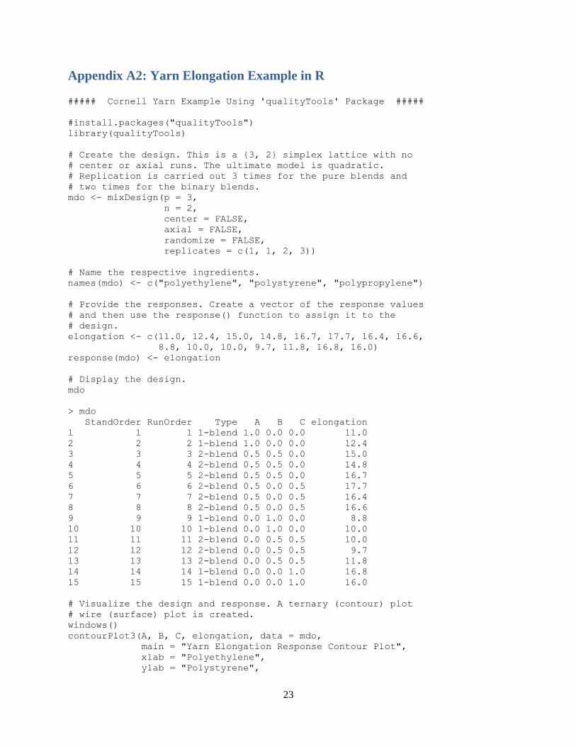
Appendix A2: Yarn Elongation Example in R
##### Cornell Yarn Example Using 'qualityTools' Package #####
#install.packages("qualityTools")
library(qualityTools)
# Create the design. This is a {3, 2} simplex lattice with no
# center or axial runs. The ultimate model is quadratic.
# Replication is carried out 3 times for the pure blends and
# two times for the binary blends.
mdo <- mixDesign(p = 3,
n = 2,
center = FALSE,
axial = FALSE,
randomize = FALSE,
replicates = c(1, 1, 2, 3))
# Name the respective ingredients.
names(mdo) <- c("polyethylene", "polystyrene", "polypropylene")
# Provide the responses. Create a vector of the response values
# and then use the response() function to assign it to the
# design.
elongation <- c(11.0, 12.4, 15.0, 14.8, 16.7, 17.7, 16.4, 16.6,
8.8, 10.0, 10.0, 9.7, 11.8, 16.8, 16.0)
response(mdo) <- elongation
# Display the design.
mdo
> mdo
StandOrder RunOrder Type A B C elongation
1 1 1 1-blend 1.0 0.0 0.0 11.0
2 2 2 1-blend 1.0 0.0 0.0 12.4
3 3 3 2-blend 0.5 0.5 0.0 15.0
4 4 4 2-blend 0.5 0.5 0.0 14.8
5 5 5 2-blend 0.5 0.5 0.0 16.7
6 6 6 2-blend 0.5 0.0 0.5 17.7
7 7 7 2-blend 0.5 0.0 0.5 16.4
8 8 8 2-blend 0.5 0.0 0.5 16.6
9 9 9 1-blend 0.0 1.0 0.0 8.8
10 10 10 1-blend 0.0 1.0 0.0 10.0
11 11 11 2-blend 0.0 0.5 0.5 10.0
12 12 12 2-blend 0.0 0.5 0.5 9.7
13 13 13 2-blend 0.0 0.5 0.5 11.8
14 14 14 1-blend 0.0 0.0 1.0 16.8
15 15 15 1-blend 0.0 0.0 1.0 16.0
# Visualize the design and response. A ternary (contour) plot
# wire (surface) plot is created.
windows()
contourPlot3(A, B, C, elongation, data = mdo,
main = "Yarn Elongation Response Contour Plot",
xlab = "Polyethylene",
ylab = "Polystyrene",

24
zlab = "Polypropylene",
form = "quadratic")
windows()
wirePlot3(A, B, C, elongation, data = mdo,
main = "Yarn Elongation Response Wire Plot",
xlab = "Polyethlyene",
ylab = "Polystyrene",
zlab = "Polypropylene",
form = "quadratic",
theta = -170)

25
### END ###

26
Appendix A3: Yarn Elongation Example in SAS
The following code is used to upload the yarn elongation experimental data into a SAS data file.
Thereafter, use the built-in ADX system to analyze the mixture data. Other types of mixture designs, such
as simplex-centroid and augmented designs follow the same general setup.
***** Mixture Design: Simplex Lattice Yarn Elongation Experiment *****;
* Load the data into a SAS data file for anlaysis in ADX;
DATA YarnElongation;
INFILE 'C:\Users\Owner\Desktop\YarnElongation.csv'
DLM = ',' FIRSTOBS = 2;
INPUT X1 X2 X3 Elongation;
RUN;
/***********************************************************************/
/* Start ADX by going to Solutions > Analysis > Design of Experiments. */
/* You have to import the data into ADX to create your design and */
/* analysis. When in ADX, go to File > Import Design and follow the */
/* prompts. */
/***********************************************************************/

27
Appendix B: Optimal Design Analysis in SAS ***** Optimal Design: D-Optimal Experiment *****;
* Create a candidate set of 125 points using do loops.;
DATA In;
DO X1 = -1 TO 1 BY 0.5;
DO X2 = -1 TO 1 BY 0.5;
DO X3 = -1 TO 1 BY 0.5;
OUTPUT;
END;
END;
END;
/*
Run the Optex procedure with the candidate set. The model, design point ;
method, criterion, and maximum iterations per cycle are specified.
The design with the highest D-value is displayed in the output window.
*/
PROC OPTEX DATA = In;
EXAMINE DESIGN;
MODEL X1 | X2 | X3@2 X1*X1 X2*X2 X3*X3;
GENERATE METHOD = FEDOROV CRITERION = D ITER = 32;
RUN;

28
The OPTEX Procedure
Average
Prediction
Design Standard
Number D-Efficiency A-Efficiency G-Efficiency Error
ƒƒƒƒƒƒƒƒƒƒƒƒƒƒƒƒƒƒƒƒƒƒƒƒƒƒƒƒƒƒƒƒƒƒƒƒƒƒƒƒƒƒƒƒƒƒƒƒƒƒƒƒƒƒƒƒƒƒƒƒƒƒƒƒƒƒƒƒƒƒƒƒ
1 46.3992 25.3479 90.8665 0.6681
2 46.3992 25.3479 90.8665 0.6681
3 46.3992 25.3479 90.8665 0.6681
4 46.3992 25.3479 90.8665 0.6681
5 46.3992 25.3479 90.8665 0.6681
6 46.3992 25.3479 90.8665 0.6681
7 46.3992 25.3479 90.8665 0.6681
8 46.3992 25.3479 90.8665 0.6681
9 46.3992 25.3479 90.8665 0.6681
10 46.3992 25.3479 90.8665 0.6681
11 46.3992 25.3479 90.8665 0.6681
12 46.3992 25.3479 90.8665 0.6681
13 46.3992 25.3479 90.8665 0.6681
14 46.3992 25.3479 90.8665 0.6681
15 46.3992 25.3479 90.8665 0.6681
16 46.3992 25.3479 90.8665 0.6681
17 46.3992 25.3479 90.8665 0.6681
18 46.3992 25.3479 90.8665 0.6681
19 46.3992 25.3479 90.8665 0.6681
20 46.3992 25.3479 90.8665 0.6681
21 46.3992 25.3479 90.8665 0.6681
22 46.3992 25.3479 90.8665 0.6681
23 46.3992 25.3479 90.8665 0.6681
24 46.3992 25.3479 90.8665 0.6681
25 46.3074 26.1841 81.3198 0.6590
26 46.3074 26.1841 81.3198 0.6590
27 46.3074 26.1841 81.3198 0.6590
28 46.3074 26.1841 81.3198 0.6590
29 46.3074 26.1841 81.3198 0.6590
30 46.3074 26.1841 81.3198 0.6590
31 46.3074 26.1841 81.3198 0.6590
32 46.3074 26.1841 81.3198 0.6590

29
The OPTEX Procedure
Examining Design Number 1
Log determinant of the information matrix 2.2278E+01
Maximum prediction variance over candidates 0.6056
Average prediction variance over candidates 0.4464
Average variance of coefficients 0.1973
D-Efficiency 46.3992
A-Efficiency 25.3479
Point
Number X1 X2 X3
ƒƒƒƒƒƒƒƒƒƒƒƒƒƒƒƒƒƒƒƒƒƒƒƒƒƒƒ
1 -1 -1 -1
2 -1 -1 0
3 -1 -1 1
4 -1 0 0
5 -1 1 -1
6 -1 1 -1
7 -1 1 1
8 -1 1 1
9 0 -1 -1
10 0 -1 1
11 0 0 -1
12 0 1 0
13 1 -1 -1
14 1 -1 0
15 1 -1 1
16 1 0 -1
17 1 0 1
18 1 1 -1
19 1 1 0
20 1 1 1

30
Works Cited Borkowski, John J. John's Home Page. n.d. Web. 3 October 2014. <www.math.montana.edu/~jobo/>.
—. John's Home Page. n.d. Web. 29 March 2015.
<http://www.math.montana.edu/~jobo/thaidox/sec14.pdf>.
Cornell, John A. "An Historical Perspective." Cornell, John A. Experiments with Mixtures: Designs,
Models, and the Analysis of Mixture Data. 2nd. New York: John Wiley & Sons, Inc., 1990. 16-
18. Print.
Lawson, John and Cameron Willden. mixexp: Design and Analysis of Mixture Experiments. R package
version 1.2.1. 2015. Software. <http://CRAN.R-project.org/package=mixexp>.
Montgomery, Douglas C. "Computer-Generated (Optimal) Designs." Montgomery, Douglas C. Design
and Analysis of Experiments. 7th. Hoboken, NJ: John Wiley & Sons, Inc., 2008. 450-459. Print.
Montgomery, Douglas C. "Mixture Experiments." Montgomery, Douglas C. Design and Analysis of
Experiments. 7th. Hoboken: John Wiley & Sons, Inc., 2008. 466-475. Print.
Myers, Richard H. and Douglas C. Montgomery. "Augmentation of Simplex Designs with Axial Runs."
Myers, Richard H. and Douglas C. Montgomery. Response Surface Methodology: Process and
Product Optimization Using Designed Experiments. New York: John Wiley & Sons, Inc., 1995.
551-558. Print.
National Institute of Standards and Technology. "I've heard some people refer to 'optimal' designs,
shouldn't I use those?". n.d. Web. 13 October 2014.
—. D-Optimal designs. n.d. Web. 13 October 2014.
—. What is a mixture design? 27 June 2012. Web. 3 October 2014.
<http://www.itl.nist.gov/div898/handbook/pri/section5/pri54.htm%5B6/27/2012>.
R Core Team. R: A language and environment for statistical computing. Vienna: R Foundation for
Statistical Computing, 2014. Software. <http://www.R-project.org/>.
Roth, Thomas. qualityTools: Statistics in Quality Science. R package version 1.54. 2012. Software.
<http://www.r-qualitytools.org>.
SAS Institute Inc. SAS OnlineDoc 9.3. Cary: SAS Institute Inc., 2011. Software.
Scheffe, Henry. "Experiments With Mixtures." Journal of the Royal Statistical Society. Wiley, 1958.
Electronic. 29 December 2014. <http://www.jstor.org/stable/2983895>.
—. "The Simplex-Centroid Design for Experiments with Mixtures." Journal of the Royal Statistical
Society. Wiley, 1963. Electronic. 29 December 2014. <http://www.jstor.org/stable/2984294>.
Wheeler, Bob. AlgDesign: Algorithmic Experimental Design. R package version 1.1-7.3. 2014. Software.
<http://CRAN.R-project.org/package=AlgDesign>.

31
Wikipedia contributors. Optimal design. Wikipedia, The Free Encyclopedia, 4 May 2015. Web. 29 March
2015. <http://en.wikipedia.org/w/index.php?title=Optimal_design&oldid=660748843>.


