Impact of Sources and Destinations

on the Observed Properties of the Internet Topology

Frederic Ouedraogoa,b,c, Clemence Magniena,b,∗

aUPMC Univ Paris 06, UMR 7606, LIP6, F-75016, Paris, FrancebCNRS, UMR 7606, LIP6, F-75016, Paris, France

cUniversity of Ouagadougou, LTIC, Ouagadougou, Burkina Faso

Abstract

Maps of the internet topology are generally obtained by measuring the routesfrom a given set of sources to a given set of destinations (with tools such astraceroute). It has been shown that this approach misses some links andnodes. Worse, in some cases it can induce a bias in the obtained data, i.e.the properties of the obtained maps are significantly different from those ofthe real topology. In order to reduce this bias, the general approach consistsin increasing the number of sources. Some works have studied the relevanceof this approach. Most of them have used theoretical results, or simulationson network models. Some papers have used real data obtained from actualmeasurement procedures to evaluate the importance of the number of sourcesand destinations, but no work to our knowledge has studied extensively theimportance of the choice of sources or destinations. Here, we use real data frominternet topology measurements to study this question: by comparing partialmeasurements to our complete data, we can evaluate the impact of addingsources or destinations on the observed properties.

We show that the number of sources and destinations used plays a role inthe observed properties, but that their choice, and not only their number, alsohas a strong influence on the observations. We then study common statisticsused to describe the internet topology, and show that they behave differently:some can be trusted once the number of sources and destinations are not toosmall, while others are difficult to evaluate.

1. Introduction

The mapping of the internet topology has received a lot of interest from theresearch community recently. Obtaining accurate maps of this topology is in-deed of key importance for several applications, including protocol simulations.

∗Corresponding authorEmail addresses: frederic.ouedraogo@univ-ouaga.bf (Frederic Ouedraogo),

clemence.magnien@lip6.fr (Clemence Magnien)

Preprint submitted to Elsevier May 5, 2010

No exact map is available due to the internet’s distributed construction andadministration, and obtaining one through measurements is a challenging task.

Efforts have been made to discover the topology at the router or ip levelby using tools such as traceroute: one collects routes from a given set ofsources to a given set of destinations, and merges them to obtain a view of thetopology. Such views give much information on the global shape of the internet.It has been shown that the internet topology has some statistical propertieswhich make it very different from most models used previously. This inducedan intense activity in the acquisition of such maps, see for instance [25, 3, 24, 12]and in their analysis, see for instance [11, 4, 12, 20, 26].

It must be clear that the image obtained in such a way is partial (somenodes and links are not seen) and may be biased by the exploration process.Several experimental and formal studies have been conducted to evaluate theaccuracy of the obtained maps of the internet, as well as the benefit of usingmore than one source (both concerning the quantity of data gathered and thebias reduction) [1, 2, 5, 7, 9, 10, 13, 14, 15, 16, 17, 21, 23, 26]. All these studiesgive good arguments of the fact that maps of the internet collected from a singlesource are very incomplete, and that there probably is a bias induced by theexploration process. This bias is greatly reduced when using more sources forthe measurement.

Using real data [18, 22] coming from recent measurements, we study in depththe differences between the ip-level maps that can be obtained from differentsources and destinations. Following a methodology introduced in [14, 15], westudy the impact of the number of sources and destinations on a number ofclassical graph properties, which allows us to determine to which extent theseproperties are biased by the exploration process. We thus confirm results previ-ously established on models. We also study the impact of the choice of sourcesand destinations on the quality of the obtained view.

We first present the data set we use and our methodology in Section 2. Wethen present in Section 3 how the choice of sources and destinations, and notonly their number, can influence the obtained view and its statistical properties.Section 4 presents our detailed analysis of the impact of the number and choiceof sources and destinations on the obtained view of the ip-level topology, bystudying classical graph properties. We discuss related work in Section 5, andpresent our conclusions in Section 6.

2. Data set and methodology

The data we use was collected in [18] and is publicly available [22]. Mea-surements were conducted from more than 150 monitors. To each monitor wasassociated a destination set that stayed the same for the whole duration of themeasurements. The measurements then consisted in periodically running thetracetree tool, which collects the routes from a given monitor to a set of des-tinations in a traceroute-like manner, but much more quickly, and imposinga far smaller load on the network. The measurements were conducted with a

2

high frequency (typically leading to about one hundred measurement rounds perday), for a long period of time (from weeks to several months, depending on themonitor). For a more comprehensive description of the measurement procedureand the obtained data, see [18].

In this original data set, all sources do not use the same destination set. Tostudy the impact of adding sources and destinations, we need to have a set ofsources running measurements towards the same destinations. In this paper, wetherefore use a data set consisting of a set S of 11 sources, which are associatedto the same set D of 3 000 destinations.

For each source j and destination k, we call gj,k the graph composed of theunion of paths from source j to destination k 1 (the union keeps only one copy ofeach link; all graphs we consider have no loops or multiple edges; moreover, alllinks are undirected and unweighted). The nodes are the ip addresses observedon the paths from source j to destination k, and the links represent the hopsat the ip level from node to node. The part of the ip-level topology observedfrom source j is then the union of what was seen from this source towards alldestinations:

gj =⋃

k

gj,k.

Notice that, in each measurement round, if a machine did not reply to aprobe, it is represented as a star (*). In a given measurement round, all starsare different. A problem arises when we perform the union of several mea-surement rounds: we cannot know if stars appearing at the same location atdifferent rounds correspond to a same machine or not. The solution we havechosen consists of not taking into account the stars or the links associated tothem in the original data set. This causes the paths from the source to somedestinations to be disconnected, and therefore the graphs gj,k may not be con-nected. However, this is not a problem for our purpose, because the graphs gjare almost connected: in all cases, the largest connected component contains atleast 92% of nodes.

All sources are not equivalent, and the sizes of the graphs gj vary. Thesmallest has 16 469 nodes, and the largest has 26 447 nodes. More details aboutthis can be found in Section 3.

From this we define the graph G to be the topology observed with all sources:G =

⋃j gj . It has n = 42 141 nodes and m = 165 438 links. Note that the nodes

of G are ip addresses and not routers, as we do not perform alias resolution.

Our approach consists generally in studying views of G obtained by exploringit using only subsets of the sources and destinations. The important point inthis study is that our data provides us with the actual paths from sources todestinations. We therefore do not rely on modeling to obtain the partial views.

1i.e. the union of the nodes and links appearing on paths from j to k in all measurementrounds. Because of load balancing and other phenomena, this path is generally not constantthroughout the whole measurement period.

3

If we denote by S′ a subset of sources and by D′ a subset of destinations,GS′D′ is the view of G obtained with theses sources and destinations, definedby:

GS′D′ =⋃

j∈S′

k∈D′

gj,k.

In the rest of the paper, we will therefore evaluate the impact of the choiceof sources and destinations by comparing different views GS′D′ , for differentsubsets S′ and D′ of the sources and destinations, with different sizes.

3. Impact of the choice of sources and destinations

In this section we evaluate the impact of both the choice and the number ofsources and destinations on the obtained view. We focus first on the number ofnodes and links of the obtained view, then on more elaborate properties.

3.1. Number of nodes and links

We focus here on the observed number of nodes and links. We will see thatthe choice of sources and destinations has a strong impact on the observations.

Studying a large number of views obtained with randomly chosen sets ofsources and destinations is computationally expensive. To solve this problemwe use the following method. When studying the impact of the choice andnumber of sources (resp. destinations), we will always build a view obtained byk sources and all destinations (resp. k destinations and all sources) by addingone source (resp. destination) to a view obtained with k − 1 sources and alldestinations (resp. k − 1 destinations and all sources). Starting with a singlesource (resp. destination) and adding sources (resp. destinations) one by oneallows us to study the impact of the number of sources (resp. destinations).Changing the order in which we consider sources (resp. destinations) allows usto study the impact of the choice of sources (resp. destinations).

A good way of evaluating the impact of the choice of sources is to investigate,given a number k of sources, what are the largest and smallest sizes (in termsof the number of nodes) of the graphs it is possible to obtain by considering ksources. We denote by Ms(k) the maximum size of a graph we can obtain withk sources:

Ms(k) = maxS′⊆S,|S′|=k

|GS′D|,

and by ms(k) the minimum size of such a graph:

ms(k) = minS′⊆S,|S′|=k

|GS′D|.

We define dually Md(k) and md(k), which are the maximum and minimumsizes of graphs that can be obtained with k destinations.

Obtaining the maximum or minimum function is too computationally ex-pensive. We therefore propose a greedy heuristic for approximating it: at each

4

0

5000

10000

15000

20000

25000

30000

35000

40000

45000

0 500 1000 1500 2000 2500 3000

M’d(k)Random maxRandom avg.Random min

m’d(k) 15000

20000

25000

30000

35000

40000

45000

0 2 4 6 8 10 12

M’s(k)Random maxRandom avg.Random min

m’s(k)

Figure 1: Left: Impact of the choice of destinations on the observed number of nodes. Right:Impact of the choice of sources on the number of nodes of the obtained view.

step we consider the graph obtained in the previous step, and choose the source(resp. destination) that adds the most nodes to this graph. We denote the sizeof the graph obtained at the k-th step by M ′

s(k) (resp. M ′d(k)). Conversely,

we approximate the minimum by starting with the source (resp. destination)that discovers the fewest nodes, and choose at each time step the source (resp.destination) that adds the least nodes to the current graph. We denote the sizeof the graph obtained at the k-th step by m′

s(k) (resp. m′d(k)).

We have no guarantee of how closeM ′s(k) andm′

s(k) are toMs(k) andms(k),but we know that they are lower and upper bounds for them, respectively.

In order to get an intuition about what we obtain when we select sources ordestinations at random, we also computed the number of nodes and links seenwith 1 000 random orders. For these orders, we computed for each number k ofsources (resp. destinations) the maximum, the minimum and the average valueobserved with the first k sources (resp. destinations).

The behaviors observed for the number of discovered nodes and links werevery similar, therefore we only present the figures concerning the number ofnodes.

Figure 1 (left) presents the impact of the chosen destinations on the observednumber of nodes. We observe several things. First, there is a high differencebetween the approximated maximum and minimum sizes M ′

d(k) and m′d(k).

For 500 destinations for instance, the observed number of nodes varies fromapproximately 7 500 to more than 25 000. This shows that, for a same numberof destinations, the choice of these destinations may have a dramatic influenceon the observed topology.

This difference is not so clear however when we consider random orders: theplots for the average, the minimum and the maximum among 1 000 orders areboth close to each other and far from the estimated maximum and minimumorders. This seems to indicate that, concerning the number of nodes, there aresome atypical orders yielding very different results from the average, but thatmost orders are close to the average and that it is therefore representative.

Figure 1 (right) shows the impact of the chosen sources on the observed

5

number of nodes. As for the destinations, the difference between the minimumand the maximum is important: when considering 4 sources, the number ofobserved nodes varies from 64% to 91% of the whole graph.

However, we can see that the maximum value observed for 1 000 randomorders is equal to M ′

d(k); in the same way, the minimum value observed isequal to m′

d(k). The fact that we consider a small number of sources plays animportant role in this. Though the number of orders we consider is very smallcompared to the total number of possible orders on 11 sources (1 000 comparedto 11! ∼ 40 · 106), the probability of observing the actual maximum for smallnumbers of sources is very high. For k = 3 sources for instance, the probabilityof not observing Ms(3) is equal to 0.2% approximately 2.

Our observations are in accordance with previous work [5] about the impactof the number of sources and destinations on the observed number of nodesand links. However, the authors had considered the greedy maximum order forsources, and a random order for destinations. Their conclusions were that thereis a diminishing returns effect concerning sources: adding sources provides lessand less additional information. Adding destinations, on the other hand, givesan approximately constant benefit.

The authors of [26] have mitigated the diminishing returns effect. They arguethat, even though adding sources brings less additional information on average,the benefit of adding many sources is far from negligible. They considered alarge number of sources, and sorted them by decreasing order of the numberof links they discover. Notice however that this order is naturally close to thegreedy maximum order.

By comparing the greedy maximum and minimum orders as well as ran-dom orders, both for sources and destinations, we conclude that the effect ofadding sources and destinations is similar. We observe a strong diminishingreturns effect for the greedy maximum orders: in this case, the last sources ordestinations bring very little new information. This effect does not appear forthe greedy minimum orders, for which the plots are approximately linear. Thequestion of whether we would observe a diminishing returns effect for the greedyminimum order if more sources or destinations were used remains open, but weconjecture that the linear shape of the plot is caused by an intrinsic hetero-geneity in the number of nodes each source or destination discovers. Finally,the average orders represent what one may expect to observe in practice. Thediminishing returns effect is present, but much less striking than for the greedymaximum orders. In particular, while the first sources or destinations discovermore nodes that the others, adding more sources or destinations still brings anapproximately linear benefit. Extreme behaviors, leading to the observation ofmuch more (or much less) nodes than expected, happen much more often forsources than destinations. This is linked in part to the fact that we use less

2The probability for a given order to not select the three sources that give Ms(3) is p =1 − 3!/(11 ∗ 10 ∗ 9), and p1000 ∼ 0.2%. The same probability applies when considering 8sources.

6

Average degree # sources # dest. Global Clust. # sources # dest.

7.852343 11 2993 0.160401 1 2447.856401 11 2976 0.256501 1 57.855130 11 2975 0.125881 3 3587.853955 11 2914 0.496428 1 3537.852128 11 2997 0.152805 5 287.854578 11 2976 0.250000 1 17.854771 11 2984 0.154679 2 2447.891898 11 2934 0.131765 4 3967.853233 11 2973 0.185765 2 37.853207 11 1996 0.136787 3 503

Original graph G7.851641 11 3 000 0.101155 11 3 000

Table 1: Maximum values of the average degree and the global clustering reached with 10different orders on sources and destinations. For each order, we report the maximal valuesobserved over all graphs GS′D′ obtained with the first |S′| sources and |D′| destinations inthe order.

sources than destinations.Finally, we conclude that the number of sources and destinations as well as

their choice plays an important role on the size of the observed topology.

3.2. Other properties

We now study the impact of the choice of sources and destinations on otherproperties. Given an order on sources and one on destinations, we build allgraphs GS′D′ obtained with the first |S′| sources and |D′| destinations in theorders. We then compare the observations for different orders.

Table 1 shows the maximum values observed for the average degree 3 and theglobal clustering 4 for 10 different random orders on sources and destinations.We observe that the maximum is different for all orders. In the case of the globalclustering, the difference can be quite high: the observed values vary from 0.13to 0.5. Moreover, the number of sources and destinations for which it is reachedvaries also. This means that, for a given number of sources and destinations,their actual choice can have a strong impact on the observed properties. Thoughthe maximal value is not representative of all that can be observed for a givenorder, this already brings to light strong differences in the observations fordifferent orders.

Notice that the average degree presents much less variation: the maximalvalues observed are all close to each other, and are obtained for similar numbers

3d◦ = 2m/n, see Section 4.1.4gc is equal to three times the number of triangles, divided by the number of connected

triples, see Section 4.2.

7

of sources and destinations. This shows that not all properties are affected in thesame way by the choice of sources and destinations, and that some propertiescan probably be trusted more than others.

4. Grayscale plots

We now turn to a more detailed study of the impact of the choice of sourcesand destinations on the observed properties. To study this impact on a givenproperty 5 p, we use grayscale plots as introduced in [14, 15]. We consider arectangle of width |D| and height |S|. Given an order on sources and one ondestinations, each point (d, s) of the rectangle corresponds to the graph GS′D′

such that S′ contains the first s sources in the order, and D′ contains the firstd destinations. The point is drawn using a grayscale representing the value ofp: from black for p = 0 to white for the maximal observed value of p (whichmight be greater than the value obtained for the whole graph G). The pointsdarker than the upper-right point correspond to conditions where the value p isunderestimated, whereas lighter points correspond to conditions in which it isover-estimated. The gray variation is linear: if a dot is twice as dark as anotherdot, then the associated value is twice as large.

Finally, to improve readability, we represent level lines. The l-level line isdefined as the set of points where the value of p over its maximal value is betweenl − 0.01 and l + 0.01. The 0.1-level line is represented in white, the 0.5-levelline alternates black and white segments, and the 0.9-level line is represented inblack 6.

The fact that the graph corresponding to the point (d−1, s−1) is included inthe one corresponding to (d, s) quickens considerably the computations neededto produce such plots.

Since, as already discussed, the choice of sources and destinations has aninfluence on the observed properties, different orders will produce differentgrayscale plots. Generating plots for different orders, as well as the averageplot obtained with several orders, will therefore help us in evaluating this im-pact.

We now turn to the study of important graph statistical properties. For eachproperty, we will recall its definition, then study grayscale plots corresponding todifferent orders to evaluate the impact of the number of sources and destinations(and the impact of their choice) on the observations.

4.1. Average degree and density

The degree d◦(v) of a node v is its number of links, or equivalently, itsnumber of neighbors. The average degree d◦ of a graph is the average of the

5All properties we consider in this paper are real-valued and non-negative.6Notice that on some plots these lines do not appear, because the variation of the value of

the observed property is not large enough.

8

0.0001

0.001

0.01

0.1

1

0 500 1000 1500 2000 2500 3000

nb of srces 123456789

1011

2

3

4

5

6

7

8

0 500 1000 1500 2000 2500 3000

Figure 2: Density (left) and average degree (right) as a function of the number of destinationsconsidered (the order on destinations is a random order). Each plot corresponds to a differentnumber of sources considered. The keys for both plots are the same.

degree over all nodes:

d◦ =1

n

∑

v

d◦(v) =2m

n.

The density is the number of links in the graph divided by the total number ofpossible links:

δ =2m

n(n− 1).

The density indicates up to which extent the graph is fully connected (all linksexist). Equivalently, it gives the probability that two randomly chosen nodesare linked in the graph. There is a trivial relation between the average degreeand the density: δ = d◦

(n−1) .

This relation implies that, when the average degree is constant with respectto the graph size, the density tends to 0 when n grows.

Figure 2 (left) presents the density as a function of the number of desti-nations considered, for different number of sources. The order chosen for thedestinations is a random order. For small numbers of destinations, the numberof sources plays an important role: for 100 destinations for instance, the den-sity varies by a factor of approximately 5, depending on the number of sources.When the number of destination grows, however, the difference quickly becomesvery small. We observed the same behavior for a significant number of differentorders on the sources (figures not presented here), which indicates that theseobservations do not depend on the order in which the sources are considered.

Figure 2 (right) presents the average degree as a function of the number ofdestinations considered, for different numbers of sources. After a rather stronginitial variation, these plots seem to reach a plateau. Notice that they are notquite constant however: the plots corresponding to a small number of sourcesseem to decrease slightly as the number of destinations increases, while the plotscorresponding to a large number of sources seem to increase slightly.

A similar change is observed for the corresponding densities: for a smallnumber of destinations, considering all sources lead to a smaller density than

9

Figure 3: Average degree. Three random orders.

Figure 4: Left: number of nodes. Middle: number of links. Right: average degree. Averagegrayscale plots for 10 different random orders.

considering a smaller number of sources. Then this trend is inverted as the num-ber of destination grows, and when all destinations are considered, consideringmore sources leads to a denser graph.

This is probably due to the fact that the observed topology from one sourceto several destinations is tree-like. When one adds destinations, this addsbranches to this tree-like structure, therefore the average degree does not changemuch, but the density decreases 7. When the number of destinations is low,sources and destinations play similar roles, and adding sources or destinationsleads to a decrease of the density. When the number of destinations is high, how-ever, adding sources leads to a densification of the tree-like structure (whereasadding destinations still leads to a decrease in the density).

Figure 3 shows three grayscale plots for the average degree, correspondingto three different (random) orders on sources and destinations. As we can see,they are not identical: the gray is more uniform for the middle plot than for theother two (the 0.5-level line does not appear), which means that the estimationis more accurate: the difference between the maximum and minimum observedaverage degree is low. The number of sources and destinations needed to achievea certain precision of the estimation also varies: the left and middle plots reachthe 0.9 level line with less sources and destinations than the right plot.

Figure 4 shows the average grayscale plots on 10 different random ordersfor the number of nodes (left), the number of links (middle) and the average

7In a tree, the average degree tends to 2 as the number of nodes grows, whereas the densitytends to 0.

10

degree (right). We first observe that the plot for the average degree is similarto the plots for single orders (Figure 3), which are themselves similar to eachother (though not identical). This means that in this case, the obtained valuedoes not strongly depend on the choice of sources and destinations: for a givennumber of sources and destinations, the obtained values are more or less thesame for the three plots of Figure 3. In this case, the grayscale plot for theaverage value over 10 random orders is therefore meaningful, and representativeof what one may expect to observe in practice.

The number of nodes, links, and the average degree all increase as the numberof sources and destinations grows. This is obvious for the number of nodes andthe number of links: more sources and destinations lead to the observation ofmore nodes and links. The case of the average degree is different, as increasingthe number of sources and destinations may increase the number of links lessthan the number of nodes, causing a decrease in the average degree. Figure 2(right) shows indeed that, for a small number of sources, the average degreedecreases when the number of destinations increases. However, once at least 3sources are considered, the average degree increases both with the number ofsources and destinations.

We can see that the average degree is better estimated than the numberof nodes or links. The fact that the average degree is obtained by dividingtwo other properties (number of nodes and links) which are improved by theuse of more sources and destinations has important consequences. If the twoproperties have the same kind of bias, the quotient may not suffer from thisbias: the estimation of the average degree is good whenever the ratio betweenthe number of links and the number of nodes is accurate, even if these numbersthemselves are poorly estimated. This is in accordance with the observationsmade on models in [14, 15].

4.2. Global and local clustering

The clustering of a graph can be defined in two ways. The first definition isthe global clustering, also named transitivity ratio. This is the probability thattwo nodes are linked, given that they are both connected to a same third node:

gc =3N▽

N∨,

where N▽ denotes the number of triangles (a triangle consists of three nodesconnected by 3 links) and N∨ denotes the number of connected triples (i.e. threenodes connected by at least two links) in the graph.

The second definition is the local clustering. The local clustering of a nodev (of degree at least 2) is the probability for any two neighbors of v to be linkedtogether:

lc(v) =2.|EN(v)|

d(v).(d(v)− 1),

where EN(v) is the set of links between neighbors of v. Notice that it is thedensity of the neighborhood of v, and in this sense it captures the local density.

11

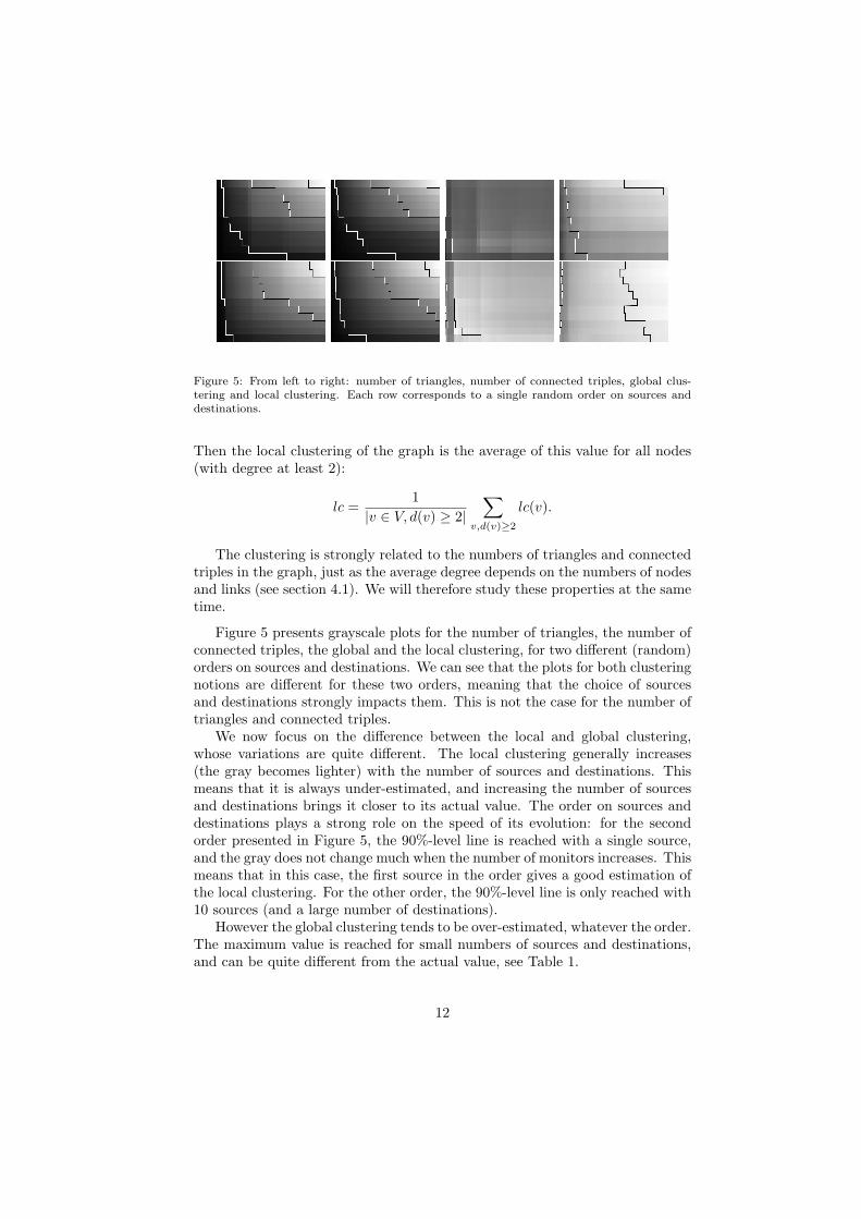
Figure 5: From left to right: number of triangles, number of connected triples, global clus-tering and local clustering. Each row corresponds to a single random order on sources anddestinations.

Then the local clustering of the graph is the average of this value for all nodes(with degree at least 2):

lc =1

|v ∈ V, d(v) ≥ 2|

∑

v,d(v)≥2

lc(v).

The clustering is strongly related to the numbers of triangles and connectedtriples in the graph, just as the average degree depends on the numbers of nodesand links (see section 4.1). We will therefore study these properties at the sametime.

Figure 5 presents grayscale plots for the number of triangles, the number ofconnected triples, the global and the local clustering, for two different (random)orders on sources and destinations. We can see that the plots for both clusteringnotions are different for these two orders, meaning that the choice of sourcesand destinations strongly impacts them. This is not the case for the number oftriangles and connected triples.

We now focus on the difference between the local and global clustering,whose variations are quite different. The local clustering generally increases(the gray becomes lighter) with the number of sources and destinations. Thismeans that it is always under-estimated, and increasing the number of sourcesand destinations brings it closer to its actual value. The order on sources anddestinations plays a strong role on the speed of its evolution: for the secondorder presented in Figure 5, the 90%-level line is reached with a single source,and the gray does not change much when the number of monitors increases. Thismeans that in this case, the first source in the order gives a good estimation ofthe local clustering. For the other order, the 90%-level line is only reached with10 sources (and a large number of destinations).

However the global clustering tends to be over-estimated, whatever the order.The maximum value is reached for small numbers of sources and destinations,and can be quite different from the actual value, see Table 1.

12

Figure 6: From left to right: number of connected triples, number of triangles, global clusteringand local clustering. Average for 10 different random orders.

Figure 6 shows (from left to right) the average grayscale plots for the numberof triangles, the number of connected triples, the global and the local clustering.The grayscale plot for the global clustering is quite uniform, which means thatthe values are very close to each other 8, independently of the number of sourcesand destinations. Therefore the global clustering seems to be well-estimated(notice that it is slightly over-estimated, as it tends to decrease when the numberof sources or destinations increase). Observations made in [14, 15] show thatthe global clustering is overestimated in graphs with low clustering when thenumber of sources is low compared to the number of destinations. In this case,explorations discover proportionally more triangles than connected triples. Thisover-estimation is not a very important one, though, therefore we expect theclustering of a topology measured with more sources and destinations to have ahigher global clustering than a random graph. We also noticed that the observedvalue for the global clustering depends strongly on the choice of sources anddestinations. Therefore, the grayscale plot for the global clustering in Figure 6is not representative of what one may obtain in practice for a single order, andthis conclusion must therefore be considered with care.

The average grayscale plot for the local clustering shows that increasing thenumber of sources and destinations makes its estimation better, as was alreadythe case for single random orders. The average behavior is therefore similarto the behaviors observed for single orders. The wide difference between theplots obtained for different orders however shows that the average plot is onlyrepresentative of the global behavior of this statistics.

In conclusion, the choice of sources and destinations influences the local andglobal clustering differently. The local clustering depends more on the numberof sources and destinations than the global clustering. Therefore it can beimproved by adding sources and destinations, even though the influence of theorder on this is very high. The global clustering is more influenced by the choiceof the sources and destinations than by their number, meaning that it is verydifficult to estimate it accurately.

The authors of [14, 15] considered only the global clustering coefficient, anddid not study the impact of the order on sources and destinations. Our observa-

8The value of the gray represents the difference with the maximum value observed for theten considered orders, which is why no white point appears.

13

Figure 7: Average distance. Left and middle: two different random orders. Right: average of10 random orders.

tions concerning average grayscale plots for the global clustering are consistentwith theirs.

4.3. Average distance

We denote by d(u, v) the distance between two nodes u and v, i.e. thenumber of links on a shortest path between them. We denote by:

d(u) =1

n− 1

∑

v 6=u

d(u, v)

the average distance from u to all nodes, and by:

d =1

n

∑

u

d(u)

the average distance in the graph.Notice that these definitions only make sense for connected graphs. In prac-

tice, if the graph is not connected (as in the present case) one generally restrictsthe computation to the largest connected component, which is reasonable sincethe vast majority of nodes are in this component. The average distance is oneof the most classical properties used to describe real-world complex networksand the internet topology in particular. Computing it is however time-costly.To quicken the computations, we use here the heuristics proposed in [17]. Itconsists in approximating the average distance by choosing at each step i a ran-dom node vi, computing its average distance to all other nodes d(vi) in timeO(m) and space O(n), and using it to improve the current approximation. The

i-th approximation of the average distance is di = 1/i∑i

j=1 d(vj). We stopas soon as the variation in the estimations becomes less than a given ǫ, i.e.|dj+1 − dj | < ǫ. The variable ǫ is a parameter allowing to tune the quality ofthe approximation vs. the computation time. We use here ǫ = 0.1.

Figure 7 presents grayscale plots for the average distance. We can see that,when one uses few sources, the average distance is over-estimated. The evalua-tion becomes more accurate when the number of sources and destinations grows.This can be understood as follows: with few sources the graph is close to a tree,

14

1

10

100

1000

10000

1 10 100 1000 1

10

100

1000

10000

1 10 100 1000 1

10

100

1000

10000

1 10 100 1000

Figure 8: Impact of the choice of sources and destinations on the degree distribution. Eachplot presents the degree distributions for three graphs GS′D′ obtained with different choicesof sources and destinations. Left: S′ contains 18% of sources and D′ 6% of destinations.Middle: S′ contains 45% of sources and D′ 26% of destinations. Right: S′ contains 81% ofsources and D′ 67% of destinations.

and the average distance is therefore over-estimated. It changes quickly whenone adds more sources.

We observe some fluctuations of the gray level for small numbers of sourcesand destinations. Once a certain number of sources and destinations is reached,the gray color becomes almost uniform, which means that the average distancedoes not vary much after this point, and that it is well estimated.

Finally, the impact of the order on sources and destinations on the averagedistance is very small. There is a strong similarity between the results fordifferent single orders. Figure 7 (left and middle) presents the grayscale plotsfor two different random orders. We can see that they are very similar, whichis also the case for other random orders we considered (not represented here).This means that the choice of sources and destinations has little impact on theobserved average distance, and that the average grayscale plot is representativeof what one may obtain in practice.

In conclusion we obtain a good estimation of the average distance as soon asa certain number of sources (and destinations) is reached. After this, the averagedistance becomes accurate and close to the original one. We also showed thatthe impact of the choice of sources and destinations on the average distance isnot important.

This is in accordance with the observations made in [14, 15] on differenttypes of graph models.

4.4. Degree distribution

The degree distribution of a graph is the fraction pk of nodes of degree ex-actly k in the graph, for all k 9. Degree distributions may be homogeneous (allthe values are close to the average, like in Poisson and Gaussian distributions),or heterogeneous (there is a huge variability among degrees, with several ordersof magnitude between them). When a distribution is heterogeneous, it makessense to try to measure this heterogeneity rather than the average value. In

9Equivalently, one may study the number of nodes with degree k.

15

1e-05

0.0001

0.001

0.01

0.1

1

1 10 100 1000

50100300500800

1000150020002500

orginal

1e-05

0.0001

0.001

0.01

0.1

1

1 10 100 1000

123456789

10original

1e-05

0.0001

0.001

0.01

0.1

1

1 10 100 1000

1-502-1003-3004-5005-800

6-10007-15009-2000

10-2500original

Figure 9: Impact of the number of sources and destinations on the degree distribution. Left:degree distributions of graphs GSD′ for which the number of destinations d = |D′| variesfrom 100 to 3 000 (all 11 sources are considered). Middle: degree distributions of graphsGS′D for which the numbers of sources s = |S′| varies from 1 to 11 (all 3 000 destinationsare considered). Right: degree distributions of graphs GS′D′ for which both the number ofsources and the number of destinations vary.

some cases, this can be done by fitting the distribution by a power-law, i.e. adistribution of the form pk ∼ k−α. The exponent α may then be consideredas an indicator of how heterogeneous the distribution is. As fitting distribu-tions to power-law leads to disputable results when the distribution is not aperfect power-law, we will however not attempt it here. We will therefore studywhether the observed distributions are heterogeneous or not, and whether theyare similar to each other.

The degree distribution of the internet is one of the properties for which thebias induced by the exploration has been the most widely studied [1, 2, 6, 7, 8, 9,10, 16, 17, 21, 23]. Certainly one of the most surprising results is from [16] whichshows that power-law distributions can be observed by performing traceroute

explorations on graphs with an underlying topology following a Poisson degreedistribution. The authors of [14, 15] deepen this result by considering severalnetwork models and varying the number of sources and destinations. They showthat this observation depends of 2 parameters: the underlying topology and thenumber of sources used to explore it. The exploration of a random graph witha few sources may indeed lead to the observation of a heterogeneous degreedistribution. This effect tends to disappear quickly when the number of sourcesgrows. However even a small number of sources in a topology with a power-lawdegree distribution provides a power-law degree distribution.

We first show to which extent the choice of sources and destinations influ-ences the observed degree distribution. Figure 8 shows the degree distributionsfor different numbers of sources and destinations. For each case, we presentthe distributions obtained with three different random choices of sources anddestinations. For small numbers of sources and destinations (Figure 8, left), weobserve a difference only for degrees larger than ten, whereas for low degrees thedistributions are almost identical. When the number of sources and destinationsincreases (Figure 8, middle and right), these distributions tend to become verysimilar for all values of the degree. This shows that the choice of sources anddestinations does not influence much the observed degree distribution, providedtheir number is not too small.

16

Since the choice of sources and destinations does not influence much theobtained degree distribution, we can now study the impact of the number ofsources and destinations, without worrying about their choice. We increase thenumber of sources and destinations separately to show their impact on the degreedistribution. Figure 9 shows the degree distributions for graphs in which we varythe number of destinations (left), the number of sources (middle), and both atthe same time (right). The first observation is that these degree distributionare all heterogeneous and do not vary greatly. This confirms observations madeby simulations in [14, 15].

The distributions of Figure 9 (left) coincide more precisely than the others.This indicates that the degree distribution is more accurately estimated whenthe number of sources is high. In this case, changing the number of destinationsdoes not alter the distribution much.

The distributions of Figure 9 (middle and right) converge to the degree dis-tribution of the final graph as the number of sources and destinations increases.Since we saw that the number of destinations does not play a great role in thedegree distributions, this means that the change is driven by the number ofsources.

In summary, we have a good approximation of the degree distributions, evenwith a small number of sources and destinations. It becomes even more accurateas the number of sources grows. It is important to notice that in all cases, theobserved degree distribution is heterogeneous. This confirms observations madeby simulations [14, 15].

5. Related work

Since a few years, many works have conducted experimental and formalstudies to evaluate the accuracy of the obtained maps of the internet. Most ofthese studies focus on the impact of the measurement procedure on the obtaineddegree distribution, and use models for the topology and the traceroute ex-ploration to evaluate this [1, 2, 6, 7, 8, 9, 10, 14, 15, 21, 23]. They give goodarguments for the fact that the maps of the internet collected with a singlesource are very incomplete, and probably suffer from an important bias. Manyof these works agree that increasing the number of sources quickly reduces thisbias, at least concerning the degree distribution.

Some works have addressed specifically the question of the impact of thenumber of sources and destinations on the obtained data: [5] and [26] study thenumber of nodes and links discovered as a function of the number of sourcesand destinations used for the exploration. They both exhibit a diminishingreturns effect, each new source adding less information than the previous one.As explained in Section 3, both papers added sources approximately in the ordergiven by the greedy maximum heuristics. Studying also random orders allowedus to moderate their observations. [14, 15] study the impact of the degrees ofsources and destinations on the observed number of nodes and links.

17

The authors of [26] study the impact of the number of sources on a number ofgraph properties, using data collected from the distributed measurement projectDimes [24]. They consider sources by decreasing order of the number of linksthey discover, and do not consider the impact of the choice of sources on theseproperties.

The grayscale plots were introduced in [14, 15] in order to obtain an in-depthunderstanding of the impact of the number of sources and destinations on a num-ber of widely studied graph properties. They used models for different types ofnetworks in order to study the impact of the network topology on the observa-tions. [5] also used contour plots, which are somewhat similar to grayscale plots,for studying the impact of the number of sources and destinations on the ob-served number of nodes and links. Our contribution is complementary to theseworks in two ways: first, we use real data, whereas these works study modelsboth for the networks and the traceroute exploration ([5] uses real data butonly studies the observed number of nodes and links); second, in this paper westudy not only the impact of the number of sources and destinations, but alsotheir choice.

Finally, some works propose empirical criteria for identifying whether theobserved properties can be trusted [17, 14, 15, 26, 16]. This is similar to ourapproach.

6. Conclusion

We conducted an extensive set of experiments aimed at evaluating the impactof the sources and destinations used in traceroute-like measurements on theproperties of the observed topology. Our goal was to estimate whether theobserved properties are the actual properties of the topology, or if they arebiased by measurement artifacts.

We used real data obtained from traceroute-like measurements, so ourresults do not rely on simulations. This has the advantage that we did notneed to rely on models, either for the internet topology, of for the traceroute

measurements.As expected from previous work in this area, we showed that the number

of sources and destinations plays a strong role on the observed properties. Wealso studied in depth the impact of the choice of sources and destinations onthe observed properties, and showed that it is important. When one uses twodifferent sets of sources and destinations with the same size, one may obtaingraphs which are very different from each other. This is true even for basicproperties such as the number of nodes and links.

We studied various graph statistics which are widely used for graph descrip-tion. We showed that they do not behave in the same way with respect tochanges in the sources and destinations used for the exploration. Some of themare strongly dependent on the choice of sources and destinations and/or theirnumber. Such properties can therefore not be trusted, since performing mea-surements with different sets of sources and destinations would lead to very

18

different results. This is the case for instance for the clustering coefficient. Onthe other hand, some properties are very resilient to changes in the sets of sourcesand destinations, and are therefore probably accurate descriptions of the actualinternet topology. This is the case for instance for the average distance and thedegree distribution.

This works could be extended in several directions. We showed that one maytrust in some properties more than in others: the average distance is probablyaccurately evaluated, while the clustering coefficient most probably is not, forinstance. This should be compared to observations on other data sets. We alsoshowed that some properties which are the ratio of two other properties maysometimes be well estimated, even if the two base properties are not accurate:if they suffer from the same bias, this bias is removed by the ratio. It wouldbe beneficial to detect other properties that can be accurately estimated. Suchproperties would probably not be ones that are classically used, since we studiedmost of these in this paper. However the fact that they can be accuratelyestimated, while more classical properties cannot be trusted, would increasetheir interest. In particular, the authors of [17] noted that the ratio betweenthe clustering coefficient and the density was probably more accurate than anyof these properties. This idea should be explored further.

We observed that different sets of sources and destinations lead to statis-tically different views of the topology. Designing methods for deciding whichsources and destinations will provide a representative view of the topology beforethe measurements start is therefore an interesting goal. This would however stillprobably require some preliminary experimental measurements, as some priorknowledge seems necessary in order to know how different sources will comple-ment each other. Since the choice of sources is limited by the fact that onemust have access to the corresponding computers, a relevant approach might beto assign different destination sets to different sources, in order to increase thecontribution of each source to the global representativeness.

Finally, the internet topology is not a static object, and it evolves with time,see for instance [19]. Performing several rounds of measurements, as was done forthe data we use here, therefore aggregates up-to-date data with obsolete data.This has certainly an impact on the properties of the obtained topology (forinstance, one may expect that it increases the density of the obtained graphs).Taking this dynamics into account in the evaluations of the properties of theobserved topology is therefore an important question.

References

[1] D. Achlioptas, A. Clauset, D. Kempe, and C. Moore. On the bias of tracer-oute sampling; or, power-law degree distributions in regular graphs. InACM Symposium on Theory of Computing (STOC2005), 2005.

[2] D. Achlioptas, A. Clauset, D. Kempe, and C. Moore. On the bias of tracer-oute sampling. Journal of the ACM, 56(4):1–28, 2009.

19

[3] Caida – archipelago project. http://www.caida.org/projects/ark/.

[4] A.-L. Barabasi and R. Albert. Emergence of scaling in random networks.Science, 286:509–512, 1999.

[5] Paul Barford, Azer Bestavros, John Byers, and Mark Crovella. On themarginal utility of network topology measurements. In Proceedings of the1st ACM SIGCOMM Workshop on Internet Measurement, in conjunctionwith Internet Measurement Conference, 2001.

[6] Qian Chen, Hyunseok Chang, Ramesh Govindan, Sugih Jamin, ScottShenker, and Walter Willinger. The Origin of Power-Laws in InternetTopologies Revisited. In IEEE Infocom. IEEE, 2002.

[7] A. Clauset and C. Moore. Accuracy and scaling phenomena in internetmapping. Phys. Rev. Lett, 2005.

[8] R. Cohen, M. Gonen, and A. Wool. Bounding the bias of tree-like samplingin IP topologies. Networks and Heterogeneous Media, 3:323 – 332, 2008.

[9] R. Cohen and D. Raz. The Internet Dark Matter - on the Missing Links inthe AS Connectivity Map. In Proceedings of IEEE INFOCOM 2006. 25THIEEE International Conference on Computer Communications, pages 1–12,April 2006.

[10] L. Dall’Asta, J.I. Alvarez-Hamelin, A. Barrat, A. Vazquez, and A. Vespig-nani. A statistical approach to the traceroute-like exploration of networks:theory and simulations. In Workshop on combinatorial and AlgorithmicAspects of Networking (CAAN), 2004.

[11] Michalis Faloutsos, Petros Faloutsos, and Christos Faloutsos. On power-lawrelationships of the Internet topology. In SIGCOMM. ACM, 1999.

[12] R. Govindan and H. Tangmunarunkit. Heuristics for internet map discov-ery. In IEEE INFOCOM 2000, pages 1371-1380, Tel Aviv, 2000.

[13] J.-L. Guillaume and M. Latapy. Complex networks metrology. In Complexsystems, 2005.

[14] J.-L. Guillaume and M. Latapy. Relevance of massively distributed ex-plorations of the internet topology: Simulation results. In IEEE infocom,2005.

[15] Jean-Loup Guillaume, Matthieu Latapy, and Damien Magoni. Relevanceof massively distributed explorations of the internet topology: Qualitativeresults. Computer Networks, 50 (16):3197–3224, 2006.

[16] A. Lakhina, J. Byers, M. Crovella, and P. Xie. Sampling biases in IPtopology measurements. In IEEE INFOCOM, 2003.

20

[17] M. Latapy and C. Magnien. Complex network measurements: Estimatingthe relevance of observed properties. In IEEE infocom, 2008.

[18] M. Latapy, C. Magnien, and F. Ouedraogo. A radar for the inter-net. In Proc. first International Workshop on Analysis of Dynamic Net-works (ADN), in conjunction with IEEE ICDM 2008, 2008. Available athttp://arxiv.org/abs/0807.1603.

[19] Clemence Magnien, Frederic Ouedraogo, Guillaume Valadon, and MatthieuLatapy. Fast Dynamics in Internet Topology: Observations and First Ex-planations. In 2009 Fourth International Conference on Internet Monitor-ing and Protection, pages 137–142. IEEE, 2009.

[20] Damien Magoni and Mickael Hoerdt. Internet core topology mapping andanalysis. Computer Communications, 28(5):494–506, 2005.

[21] T. Petermann and P. De Los Rios. Exploration of scale-free networks. Eur.Phys. J. B, 38(2), 2004.

[22] Radar program and data. http://www-rp.lip6.fr/~latapy/Radar.

[23] P. De Los Rios. Exploration bias of complex networks. In Proceedings of the7th conference on Statistical and Computational Physics Granada, 2002.

[24] Y. Shavitt and E. Shir. DIMES: Let the internet measure itself. ACMSIGCOMM Computer Communication Review, 35(5), 2005. See http:

//www.netdimes.org.

[25] Caida – skitter project. http://www.caida.org/tools/measurement/

skitter/.

[26] Udi Weinsberg and Yuval Shavitt. Quantifying the importance of vantagepoints distribution in internet topology measurements. In Proceedings ofIEEE Infocom, 2009.

21