dorothea bahns- the shuffle hopf algebra and quasiplanar wick products

8/3/2019 Dorothea Bahns- The shuffle Hopf algebra and quasiplanar Wick products

http://slidepdf.com/reader/full/dorothea-bahns-the-shuffle-hopf-algebra-and-quasiplanar-wick-products 1/16

a r X i v : 0 7 1 0

. 2 7 8 7 v 1

[ m a t h . Q A

] 1 5 O c t 2 0 0 7

The shuffle Hopf algebra and quasiplanar Wick

products

Dorothea Bahns ∗

October 15, 2007

Abstract

The operator valued distributions which arise in quantum field theory

on the noncommutative Minkowski space can be symbolized by a general-

ization of chord diagrams, the dotted chord diagrams. In this framework,

the combinatorial aspects of quasiplanar Wick products are understood

in terms of the shuffle Hopf algebra of dotted chord diagrams, leading to

an algebraic characterization of quasiplanar Wick products as a convolu-

tion. Moreover, it is shown that the distributions do not provide a weight

system for universal knot invariants.

1 Introduction

Tensor products of the operator valued distributions that appear in quantum

field theory are in general ill-defined when pulled back to the diagonal, andthe process of renormalization is necessary to define products which are well-defined distributions. For products of free field operators, the renormalizationprocedure leads to what is called the Wick product of quantum fields.

In [1], the quasiplanar Wick products were defined as a generalization of Wick products which is suitable for products of quantum fields on the noncom-mutative Minkowski space. The definition is based on a certain notion of localityand it is the first step towards a full renormalization theory in the Minkowskiannoncommutative framework. This paper elaborates on the quasiplanar Wickproducts’ combinatorial and algebraic aspects, leaving the functional analyticaspects aside. Its first aim is to clarify that the graphs we used in [1, 2] tohandle the combinatorics of quasiplanar Wick products, are a generalization of the classic chord diagrams studied e.g. in knot theory [3, 4].

Chord diagrams carry a cocommutative Hopf structure, and it is natural totry to reformulate the combinatorial aspects of quasiplanar Wick products inthis algebraic language, much in the spirit of [5]. So, the paper’s second aim is to

∗Department Mathematik, Universitat Hamburg, Bundesstr. 55, D - 20146 Hamburg,Germany — [email protected]

1

http://arxiv.org/abs/0710.2787v1






































reformulate the combinatorial aspects of quasiplanar Wick products as provedin [1, 2] in this algebraic setting and to show that the Hopf structure with the

shuffle product and deconcatenation coproduct is the natural one in our context.A completely algebraic characterization of quasiplanar Wick products in termsof a convolution in the shuffle Hopf algebra is given in section 4. Section 5is devoted to explicitely relating these algebraic objects and relations to theoperator valued distributions which arise in quantum field theory on the non-commutative Minkowski space. In the last section, it is shown that, althoughthese distributions bear some similarity with weight systems [4], they do notfulfill the 4T relation.

2 Dotted chord diagrams

Let us first recall the notion of a chord diagram. Let L denote a directed simplepolygonal arc in [0, 1] × R, let ∂L denote its boundary, that is, the set of itstwo endpoints. A chord diagram on L is a finite set of ordered pairs of distinctpoints on L\∂L. The pairs of points are usually symbolized by connecting lines,

the chords of the chord diagram, whose shape is irrelevant, e.g. q q q q- forthe set {(x1, x3), (x2, x4)}, where x1, x2, x3, x4 appear on the arc from left toright in that order.

Definition 1 Let L be an arc. A dotted chord diagram on L is a finite set of ordered pairs of points on L \ ∂L.

Observe that in this definition, we admit pairs (x, x) of nondistinct points.We refer to such pairs as dots. We continue to symbolize a pair of distinct pointsby its connecting line and symbolize a pair (x, x) on the arc simply by the point

x itself, e.g. q q q q q- for a set {(x1, x3), (x2, x5), (x4, x4)} with xi = xj fori = j and where x1, x2, x3, x4, x5 appear on the arc from left to right in thatorder. Observe that a dotted chord diagram that only contains pairs of distinctpoints is indeed a chord diagram in the usual sense. These diagrams thus appearas special cases of dotted chord diagrams and will be called diagrams withoutdots. Likewise, we will call the dotted chord diagrams containing only pairs of non-distinct points diagrams without chords or chordless diagrams.

We say that a dotted chord diagram has dot-degree m, and write ddeg(D) =m, if its pairs are built from m distinct points on the arc. For example, the twodotted diagrams above have dot-degree 4 and 5, respectively. Note that usually,the degree of a chord diagram is the number of its chords, hence, the dot-degreeof a chord diagram without dots is twice the ordinary degree.

Let V m denote the finite dimensional vector space that is spanned overC

byall dotted chord diagrams of dot-degree m, and let V = m≥0 V m with V 0 = C.

It is well known that the vector space of chord diagrams forms a Hopf algebra,see for instance [4]. We will generalize this structure to the vector space of dottedchord diagrams. The unique way to glue together two directed arcs L1 and L2

(in that order from left to right), such that the resulting arc is again directed,

2



extends by linearity to an associative product µ : V ⊗V → V . Usually, we writea

·b or ab for µ(a

⊗b). The unit for this product is the empty diagram -

which we also denote by ∅ or 1. Now consider the coproduct ∆ : V → V ⊗ V ,defined on diagrams as

∆(D) =

∅⊂D′⊂D

D′ ⊗ (D \ D′)

where the sum runs over all subdiagrams (including the empty diagram as wellas D itself). Its counit is the map ǫ that is equal to 1 on the empty diagram and

0 elsewhere, and the primitive elements in V are q- and q q- It is standardto check that (V,µ, ∆) is a bialgebra, and since V is graded and connected,it follows that V is a Hopf algebra. Its antipode is given inductively on thedot-degree of a diagram by S (∅) = ∅, and for D = ∅,

S (D) = −D − ∅D′D

S (D′) · (D \ D′)

We have, for example,

S ( q q q q-) = q q q q-+ q q q q-− q q q q-

S is an algebra-antihomomorphism, that is, S (ab) = S (b)S (a), and since ∆ iscocommutative, we have S 2 = idV , see [3].

3 The Quasiplanar Wick map

Let us recall and extend some definitions from [6] and [1], respectively. Thelabelled intersection graph of a chord diagram without dots is a graph whosevertices are the chords of D, numbered from 1 to ddeg(D)/2 in the order inwhich their starting points appear along the arc, and where two vertices areconnected by an edge iff the corresponding two chords in D intersect.

To extend this definition to dotted chord diagrams, we first establish how tolabel dotted chord diagrams. Let D be a dotted chord diagram, then we labelits chords and dots on the same footing in the order as they appear along thearc, e.g.

q q q q

3 q q q q

5

1 2 4-

Definition 2 The labelled intersection graph of a dotted chord diagram D is a

graph with coloured vertices. It is composed of the labelled intersection graph(with, say, white vertices) of the diagram D with all dots removed but keepingthe original labels of the diagram D, and an additional set of, say, black vertices,one for each dot in D, also with the labels from D. An edge connects a blackvertex with a white vertex provided that on the arc, the dot corresponding tothe black vertex is between the two endpoints of the chord corresponding to

3



the white vertex. The adjacency matrix of the labelled intersection matrix of adotted chord diagram was called the extended incidence matrix in [1]. A dotted

chord diagram is called connected if its labelled intersection graph is connected.

Example The labelled intersection graph of the dotted chord diagram q q q q q q q q- is the graph

b

1 b

2 r

3 b

4 r

5 Its adjacency matrix isa symmetric 5 × 5-matrix J with J 12 = 1, J 23 = 1.

Before reformulating the definition of quasiplanar Wick products from [1]in the present context, we need some more definitions. We first extend thedefinition of regular chord diagrams [7].

Definition 3 A dotted chord diagram is called regular , if for any two pairs of distinct points (x, y) and (w, z) in the diagram whose chords do not intersect,both x and y appear either on the right hand side or on the left hand side of

both z and w on the arc.For example, the diagram q q q q- is regular (and connected), while the

diagram q q q q- is not regular.

Definition 4 A dotted chord diagram is called quasiplanar , if for any two pairsof points (x, y) and (z, z) in the diagram, both x and y appear either on theright hand side or on the left hand side of z on the arc.

Observe that a diagram is quasiplanar if and only if its labelled intersectiongraph does not contain any edges between back and white vertices. For exam-ple, the diagram q q q q q q q q- is quasiplanar (regular, not connected),

while the diagram q q q q q q q q- is not quasiplanar (but still regular).Observe that any diagram without dots and any diagram without chords is

quasiplanar. In particular, the diagramq q q q-

is quasiplanar (but notregular).

We will now consider regular quasiplanar diagrams, and denote by V rqn thesubspace of V n that is spanned by regular quasiplanar dotted chord diagramsof dot-degree n. We also use the notation V rq =

V rqn .

Remark 5 It is not difficult to see that a product of connected quasiplanardiagrams is regular quasiplanar and that any regular quasiplanar diagram canbe written in a unique way as a product of nontrivial connected quasiplanardiagrams. More generally, any regular diagram can be written in a unique wayas a product of nontrivial connected diagrams.

For this reason, connected quasiplanar diagrams will turn out to be impor-

tant. Observe in particular, that a connected quasiplanar dotted chord diagramD is either the diagram q- or it does not contain any dots. Unless it is of dot-degree 1, a connected quasiplanar dotted diagram therefore has even dot-degree. We will denote by Dcq

n the set of all connected quasiplanar dotted chorddiagrams of dot-degree n, and by Dcq the set of all connected quasiplanar dottedchord diagrams.

4



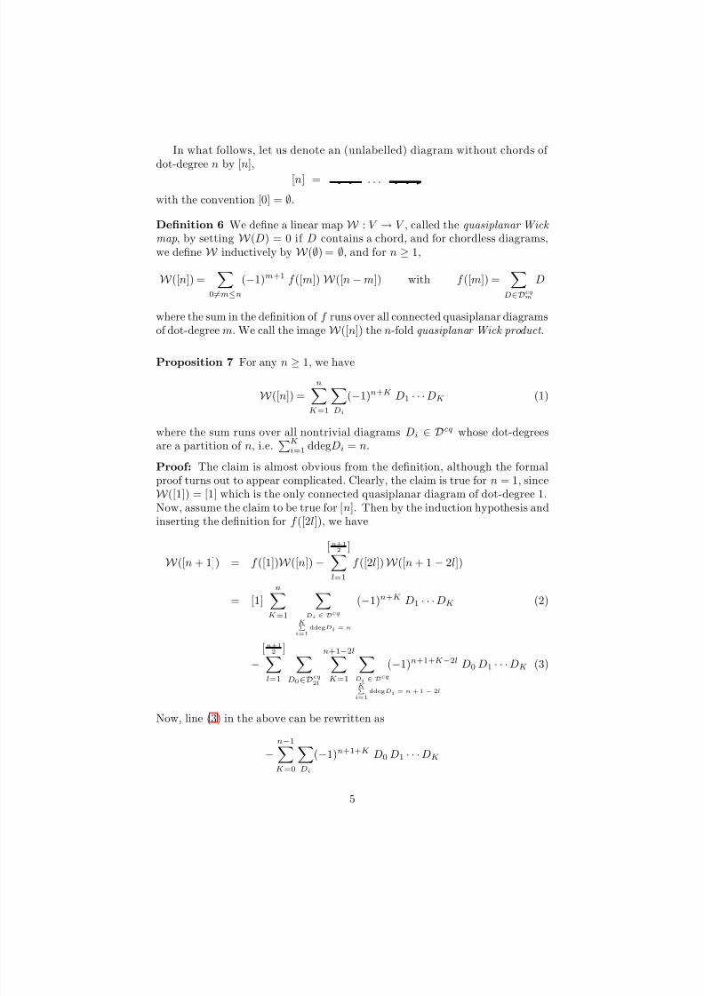
In what follows, let us denote an (unlabelled) diagram without chords of dot-degree n by [n],

[n] = q q . . . q q-

with the convention [0] = ∅.

Definition 6 We define a linear map W : V → V , called the quasiplanar Wick

map, by setting W (D) = 0 if D contains a chord, and for chordless diagrams,we define W inductively by W (∅) = ∅, and for n ≥ 1,

W ([n]) =

0=m≤n

(−1)m+1 f ([m]) W ([n − m]) with f ([m]) =

D∈Dcqm

D

where the sum in the definition of f runs over all connected quasiplanar diagramsof dot-degree m. We call the image W ([n]) the n-fold quasiplanar Wick product .

Proposition 7 For any n ≥ 1, we have

W ([n]) =n

K=1

Di

(−1)n+K D1 · · · DK (1)

where the sum runs over all nontrivial diagrams Di ∈ Dcq whose dot-degreesare a partition of n, i.e.

Ki=1 ddegDi = n.

Proof: The claim is almost obvious from the definition, although the formalproof turns out to appear complicated. Clearly, the claim is true for n = 1, sinceW ([1]) = [1] which is the only connected quasiplanar diagram of dot-degree 1.Now, assume the claim to be true for [n]. Then by the induction hypothesis and

inserting the definition for f ([2l]), we have

W ([n + 1]) = f ([1])W ([n]) −[n+1

2 ]l=1

f ([2l]) W ([n + 1 − 2l])

= [1]n

K=1

Di ∈ Dcq

KP

i=1ddegDi = n

(−1)n+K D1 · · · DK (2)

−[n+1

2 ]l=1

D0∈D

cq

2l

n+1−2lK=1

Di ∈ D

cq

KP

i=1

ddegDi = n + 1 − 2l

(−1)n+1+K−2l D0 D1 · · · DK (3)

Now, line (3) in the above can be rewritten as

−n−1K=0

Di

(−1)n+1+K D0 D1 · · · DK

5



where the second sum runs over all nontrivial diagrams D0, D1, . . . , DK ∈ Dcq

with Ki=0 ddegDi = n + 1 and ddegD0

≥2. Observe that for n even, the sum

actually starts with K = 1, since for K = 0, the second sum is empty (we wouldhave ddegD0 = n + 1, in contradiction with the fact that the dot-degree of D0

has to be even). Shifting the summation index by one, we then find that line (3)is equal to

−n

M =1

Di

(−1)n+M D1 · · · DM

where the second sum now runs over all nontrivial diagrams D1, . . . , DM ∈ Dcq

withM

i=1 ddegDi = n + 1 and ddegD1 ≥ 2. Observe that this sum can beextended to include the case M = n+1, since the sum over the diagrams is emptyin that case (since the conditions ddegD1 ≥ 2 and ddegD1 + · · · + ddegDn+1 =n + 1 cannot be fulfilled simultanously). Using that the diagram [1] is in factthe sum over all diagrams D0

∈ Dcq with ddegD0 = 1, and again shifting the

summation index, we now rewrite line (2) in the above as follows

n+1M =2

Di

(−1)n+M +1 D1 · · · DM

where the second sum runs over all nontrivial diagrams D1, . . . , DM ∈ Dcq withM i=1 ddegDi = n + 1 and ddegD1 = 1. This sum can in fact be extended to

include M = 1, since for n ≥ 1, the sum over the diagrams is empty in this caseanyway. Putting both sums together proves the proposition.

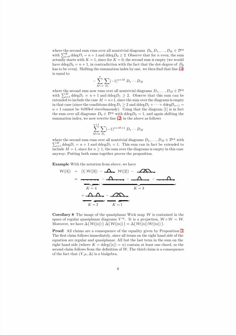
Example With the notation from above, we have

W ([4]) = [1] W ([3]) − q q- W ([2]) − q q q q-

= q q q q- K = 4

− q q q q- − q q q q- − q q q q- K = 3

+ q q q q- K = 2

− q q q q- K = 1

Corollary 8 The image of the quasiplanar Wick map W is contained in thespace of regular quasiplanar diagrams V rq . It is a projection, W ◦ W = W .Moreover, we have ∆

W ([n])

∆W ([m])

= ∆

W ([n]) W ([m])

.

Proof: All claims are a consequence of the equality given by Proposition 7.

The first claim follows immediately, since all terms on the right hand side of theequation are regular and quasiplanar. All but the last term in the sum on theright hand side (where K = ddeg([n]) = n) contain at least one chord, so thesecond claim follows from the definition of W . The third claim is a consequenceof the fact that (V,µ, ∆) is a bialgebra.

6



Proposition 9 For the product of two quasiplanar Wick products W ([n]) and

W ([m]), we find the relation

W ([n])W ([m]) = W ([n + m]) +

n+mK=1

Di

(−1)n+m+K+1 D1 · · · DK (4)

where the sum runs over all nontrivial diagrams D1, . . . , DK ∈ Dcq such thatKi=1 ddegDi = n+m but where no 1 ≤ S ≤ n+m exists, such that

Si=1 ddegDi =

n andK

i=S+1 ddegDi = m.

Proof: We write down the expressions for W ([n]), W ([m]), and W ([n + m]) ac-cording to Proposition 7. It is then not difficult to establish that all terms whichappear in the product W ([n])W ([m]) also appear in W ([n+m]). The converse isnot true; the diagrams that appear in W ([n + m]) but not in W ([n])W ([m]) arethe regular diagrams which contain chords connecting some of the first n pointswith some of the last m−n+1 points. These diagrams are of the form D1 · · · DK

with Di ∈ Dcq such thatK

i=1 ddegDi = n + m but where no 1 ≤ S ≤ n + m ex-

ists, such thatS

i=1 ddegDi = n andK

i=S+1 ddegDi = m. They each appear

with prefactor (−1)n+m+K. Subtracting all such diagrams (with their prefac-tors) from W ([n + m]) therefore yields the product W ([n])W ([m]). This provesthe proposition.

The signs which appear in equation (4) above can also be given in terms of the number of connected diagrams with dot-degree strictly larger than 1. Moregenerally, we have:

Remark 10 For any product D1 · · · DK with nontrivial diagrams Di ∈ Dcq,

and ddegDi = n, we have

(−1)n+K D1 · · · DK = (−1)d2 D1 · · · DK

where d2 is the number of connected quasiplanar diagrams in D1 · · · DK withdot-degree strictly greater than 1. To see that this is true, observe that (−1)n+K =(−1)n−K , and that K = d1 + d2, where d1 counts the number of connected dia-grams of dot-degree 1. Now, any quasiplanar connected diagram of dot-degree> 1 has even dot-degree, hence n − d1 is even, and the claim follows.

Example We have

W ([2]) W ([2]) = W ([4]) + q q q q-

K = 1

+ q q q q-

K = 3

7



and

W ([2]) W ([3]) = W ([5]) + q q q q q- + q q q q q- K = 2

− q q q q q- K = 3

+ q q q q q- K = 4

For reasons inherent to quantum field theory, it is desirable to rewrite all termson the right hand side of equation (4) in terms of the quasiplanar Wick mapW . This is achieved by first extending W to diagrams with chords. The imageof this extension is contained in the vector space of quasiplanar diagrams, butin general no longer in the vector space of regular quasiplanar diagrams. The

construction is not yet fully understood in algebraic terms and is not necessaryto understand the results presented in the remaining sections of this paper.By Proposition 7, a dotted diagram without chords [n] can obviously be

rewritten as follows

[n] = W ([n]) −n−1K=1

Di

(−1)n+K D1 · · · DK

where the sum runs over all nontrivial diagrams Di ∈ Dcq withK

i=1 ddegDi =n. We would like to iterate this process of replacing dots by Wick productsalso in diagrams containing chords (such as the terms of the sum over K in theabove).

The map

W itself cannot be used to that end, since it maps any diagram

containing a chord to 0. We now define an extension W ′ of W which is equal toW on diagrams without chords and on quasiplanar diagrams with chords actsas W on the diagram’s dots while leaving the rest of the diagram unchanged.Observe that W ′ takes values in the vector space of quasiplanar, but not neces-sarily regular diagrams, i.e. the image of W ′ is not in general contained in V rq .We again call a term of the form W ′(D), where D is a diagram, a quasiplanarWick product.

Example We have

W ′( q q q q q q- ) = q q q q q q- − q q q q q q-

− q q q q q q- − q q q q q q-

+ q q q q q q-

−q q q q q q-

Compare this with the quasiplanar Wick product W ([4]) given on page 6.

Iterating the procedure of replacing products of dots by quasiplanar Wickproducts using W ′, we can rewrite any quasiplanar dotted chord diagram D interms of elements of the image of W ′ and of diagrams without dots. This means

8



that the image of W ′ together with diagrams without dots provides a basis forquasiplanar dotted chord diagrams. The algebraic meaning of this, however,

remains to be understood.

Example The diagram q q q q q q- is equal to the sum

= W ′( q q q q q q- ) − q q q q q q- + q q q q q q-

+ q q q q q q- + q q q q q q- + q q q q q q-

= W ′( q q q q q q- ) − q q q q q q- + q q q q q q-

+ W ′( q q q q q q- ) − q q q q q q-

+ W ′( q q q q q q- ) − q q q q q q-

+ W ′( q q q q q q- ) − q q q q q q-

In particular, we can use the map W ′ to rewrite all terms on the right handside of equation (4) from Proposition 9 in terms of quasiplanar Wick products.The resulting equation is what is called the quasiplanar Wick theorem in [ 1, 2].

4 The shuffle Hopf algebra

By Corollary 8, the image of the quasiplanar Wick map W is contained inthe space of quasiplanar regular diagrams V rq . We will now consider a Hopf structure on V rq such that the quasiplanar Wick map can be understood asa convolution in this Hopf algebra. Incidentally, the ordinary Hopf algebra of chord diagrams does not seem to be natural in this context, but instead we haveto consider the Hopf structure.

By remark 5, any regular quasiplanar diagram can be uniquely written as aproduct of connected quasiplanar diagrams. We use this to endow V rq with acommutative product, the so-called shuffle product µ# : V rq ⊗ V rq → V rq ,

µ#(D ⊗ D′) =

σ∈Shn,m

Dσ(1) · · · Dσ(n+m)

where D = D1 · · · Dn and D′ = Dn+1 · · · Dn+m with Di nontrivial, quasiplanar,and connected, and where Shn,m = S n+m/S n × S m is the set of shuffle per-mutations, that is all elements σ of S n+m which leave the order of the first nelements and that of the last m elements unchanged, i.e. σ(1) < σ(2) < . . . σ(n)

and σ(n + 1) < σ(n + 2) < · · · < σ(n + m). We will usually write a#b forµ#(a ⊗ b). It is known that the shuffle product allows for a Hopf structure withthe deconcatenation product as coproduct ∆dc : V rq → V rq ⊗ V rq ,

∆dc(D) = 1 ⊗ D + D ⊗ 1 +

n−1k=1

D1 · · · Dk ⊗ Dk+1 · · · Dn

9



for D = D1 · · · Dn with Di nontrivial, quasiplanar and connected. Here, 1 de-notes the empty diagram

∅= [0] which is the unit for the shuffle product. The

counit is the map ǫ that is equal to 1 on the empty diagram and 0 elsewhere. Theantipode of this Hopf algebra is S (D1 · · · Dn) = (−1)nDn · · · D1 where the dia-grams Di are nontrivial, quasiplanar, and connected. Observe that (V, µ#, ∆dc)is a commutative non-cocommutative graded connected Hopf algebra.

Example We have

q q q q- # q q q q- =

= q q q q q q q q- + q q q q q q q q-

+ q q q q q q q q- + q q q q q q q q-

and

∆dc(q q q q q q q q-

) == 1 ⊗ q q q q q q q q- + q q q q q q q q- ⊗ 1

+ q q q q- ⊗ q q q q- + q q q q q- ⊗ q q q-

+ q q q q q q q- ⊗ q-

By definition, the primitive elements of this Hopf algebra are the connectedquasiplanar diagrams.

Proposition 11 Let h : V → V be the map defined by h([0]) = 1, h(D) = 0 forany diagram D containing chords and for any diagram of the form D = [2k +1],and let

h([n]) =

n

K=1(−1)

K Di

D1 · · · DK

for even n, where the second sum runs over all connected quasiplanar diagramsof dot-degree strictly greater than 1 with

ddegDi = n. Then the quasiplanar

Wick product on diagrams without chords is the convolution of the identity mapwith h with respect to the shuffle Hopf algebra,

W ([n]) = id ⋆ h ([n]) = µ# ◦ (id ⊗ h) ◦ ∆dc ([n])

Proof: By the definition of ∆dc, and observing that h([0]) = 1, we find

µ# ◦ (id ⊗ h) ◦ ∆dc ([n]) = µ#n

r=0

[r] ⊗ h([n − r])= µ#

1 ⊗ h([n]) + [n] ⊗ 1 +

n−1r=1

[r] ⊗ h([n − r])

10



Now, inserting the definition of h, we find for the third term

n−1r=1

[r] ⊗ h([n − r]) =n−1L=1

Di

(−1)d2 D1 . . . Dr ⊗ Dr+1 · · · DL

Here, the sum runs over all nontrivial quasiplanar connected diagrams D1, . . . , DL

with

ddegDi = n where at least one and at most n − 1 diagrams are of dot-degree 1, d2 denotes the number of diagrams with dot-degree ≥ 2, and moreover,all diagrams Di of dot-degree 1 are in the tensor product’s first entry. Observethat this last condition fixes the value of r in the above.

Application of the shuffle product µ# then yields h([n]) + [n] for the firsttwo terms and for the sum above it distributes the diagrams of dot-degree 1, i.e.the dots [1] from the tensor product’s first entry, in all possible orders betweenthe connected components of higher dot-degree. This yields all the terms that

appear on the right hand side of equation (1) in Proposition 7, and by remark 10,also the signs (−1)d2 match those appearing in equation (1). This proves theproposition.

Example For the diagram [4], we have indeed

µ#(id ⊗ h)∆dc ([4]) = µ#(id ⊗ h)(1 ⊗ q q q q- + q- ⊗ q q q- +

+ q q- ⊗ q q- +

+ q q q- ⊗ q- + q q q q- ⊗ 1)

= µ#(− 1 ⊗ q q q q- + 1 ⊗ q q q q- + 0

−q q-

⊗q q- + + 0 + q q q q-

⊗1)

= W ([4])

There is reason to hope that the extension W ′ of W can be understood in alge-braic terms in a similar manner, and that an algebraic version of the quasiplanarWick theorem can be given.

5 Relation to quantum fields on the noncommu-

tative Minkowski space

Let me now recall from [1, 2] how the graphical language of the previous sectionsencodes certain operator valued distributions of quantum field theory on thenoncommutative Minkowski space. The noncommutative Minkowski space

M θ := Cq0, q1, q2, q3/Rθ

11



is a quotient of the free algebra of 4 generators Cq0, q1, q2, q3, where Rθ is theideal defined by qµqν

−qνqµ

−iθµν I for µ, ν

∈ {0, 1, 2, 3

}with a nondegenerate

antisymmetric matrix (θµν) ∈ M (4 × 4,R). In order to define quantum fieldson M θ, it is convenient to work with the corresponding Weyl algebra generatedby the Weyl operators

eikq , where kq =3

µ=0kµ qµ with k ∈ R4 , kµ =

3ν=0

kν ηνµ , η = diag(+, −, −, −)

such that for p, k ∈ R4,

eikq eipq = e−i2kθp ei( p+k)q with kθp =

3µ,ν=0

kµ θµν pν

The signs in the symmetric form η above (the Minkowski metric) are at this

point merely a convention with no important consequences. The signature of η will, however, play a decisive role when the partial differential operators thatare relevant in field theory are considered. In fact, questions of renormalizationsubstantially depend on the signature of η, as I will show elsewhere [9].

Consider the operator valued distribution ϕ given by the free massive scalarreal Klein Gordon field. Let ω be a state (i.e. a positive linear functional) on theWeyl algebra, and let ψω denote its associated Wigner function whose Fouriertransform is ψω(k) = ω(eikq). Then the free massive scalar real Klein Gordonfield φ on quantum spacetime E is defined as an affine functional on a dense setof the state space of the Weyl algebra, with values in the endomorphisms of adense subset of Fock space, see [8], by the equation

φ(ω) = ϕ(ψω) . (5)

Let n > 0, let f be a Schwartz function on R4n, let ψnω(k1, . . . , kn) := ω(

nj=1 eikjq),

and let × denote the convolution. Then the regularized power of φ is defined by

φnf (ω) = ϕ⊗n(ψn

ω × f ) . (6)

where ϕ⊗n is the operator valued distribution in n variables, formally definedby its integral kernel ϕ⊗n(x1, . . . , xn) =

ni=1 ϕ(xi) as usual. In our graphical

language, the regularized power φnf is symbolized by a dotted diagram of dot-

degree n without chords,

φnf ↔ [n] = q q . . . q q-

We have defined a renormalization procedure [1, 2] for such powers of fields,based on a certain notion of locality, which has lead to the definition of quasi-planar Wick products. In [8] we will complete the proof that this procedure leadsto operator valued distributions that are still well-defined when the Schwartzfunction f is replaced by a δ-distribution. The functional analytic details how-ever, are not our concern here.

12



Instead, I will take the definition of quasiplanar Wick products for grantedand merely recall how the distributions which appear in that definition can be

symbolized in terms of dotted chord diagrams.Let D be a dotted chord diagram whose labelled intersection graph G has

adjacency matrix J . Let N denote the set of labels in G, let U ⊂ N and A ⊂ N denote the subsets which label the black vertices (dots) and the white vertices(chords) in G, respectively. Let f be a Schwartz function f ∈ S (R4n) which issymmetric in its arguments, f (x1, . . . , xn) = f (xπ(1), . . . , xπ(n)) for any π ∈ S n.Then the labelled intersection graph G of D determines a Schwartz functionf G ∈ S (R4u) where u = |U | by setting its Fourier transform to

f G(kU ) =

a∈A

dµ(ka) exp− i

s<t ∈N

J st ksθkt

f (kA, −kA, kU )

with the Lorentz invariant measure on the positive mass shell dµ(k), and where

for an index set I , the symbol kI abbreviates the tuple (ki)i∈I and where eachki is an element of R4. The explicit form of these integrals is

dµ(k)f (k) =

d3 p

p2 + m2−1

f (

p2 + m2 , p) for f ∈ S (R4), p ∈ R3. We extend the

correspondence D ↔ f G by linearity.The operator valued distribution corresponding to G, evaluated in a test-

function f , is then given as follows

φuf G

(ω) which by (6) is equal to ϕ⊗u(ψuω × f G) .

Observe that the socalled twisting exp − i

s<t ∈N J st ksθkt

contains prod-

ucts kuθka or kaθku where u ∈ U and a ∈ A, if and only if the dotted diagramis not quasiplanar.

Translating all graphs from Definition 6 according to the above indeed yields

the definition of quasiplanar Wick products from [1, 2]. The quasiplanarity of all terms on the right hand side of the equation in Proposition 7 means that thecorresponding distributions fulfill the locality condition requested in [1, 2].

Note that in the investigation of quantum fields on the noncommutativeMinkowski space, we also considered non-regular diagrams. It is known thatonce we admit for non-regular diagrams, a chord diagram is no longer uniquelydetermined by its labelled intersection graph. For example, the labelled inter-section graph of q q q q- is the same as that of q q q q- To distinguishsuch diagrams, we used a slightly more complicated definition of f G than the onegiven above. It is based on the use of arbitrary Schwartz functions f (which arein general not symmetric under reordering their arguments), where for a ∈ A,

the positions of the arguments ±ka in f encode the starting and end point of the chords. For instance, for the two examples above we would have

dµ(k1)dµ(k2) f (k1, k2, −k2, −k1) and

dµ(k1)dµ(k2) f (k1, −k1, k2, k2) ,

respectively. In this manner, the diagram itself, not only its labelled intersectiongraph is encoded,

D ↔ f D

13



and in particular, non-regular graphs can be distinguished. This more gen-eral definition coincides with the one given above when we consider Schwartz

functions that are symmetric under rearranging their arguments.

6 Knots

By a theorem of Kontsevich, universal properties of knot invariants of finitedegree are captured in terms of the vector space of chord diagrams modulocertain ideals given by the so-called framing independence and the 4T relation.An important tool in this framework are weight systems.

A weight system of degree m is a linear functional on the quotient of chorddiagrams of degree m modulo the framing independence and the 4T relation. Itis natural to ask whether in the special special case of diagrams without dots,the correspondence D

↔f D

, extended by linearity, defines a weight system.Unfortunately, this does not seem to be the case, as the correspondence

is not well-defined on the quotient, as the 4T relation apparently cannot besatisfied, even for modifications of the correspondence above. Let us recall thatthe framing independence relation is that an arbitrary chord diagram containingan isolated chord (i.e. one that does not intersect any other chord) is 0, andthat the 4T relation in terms of diagrams reads

q q q q- − q q q q - = q q q q - − q q q q -

= q q q q - − q q q q -

where arbitrary chords may be added in all 6 diagrams in the same positions insuch a way that the two points which are underlined remain neighbours.

We now consider the framing independence relation. Let D be a diagram(without dots) of degree n (i.e. of dot-degree 2n), let J denote the adjacencymatrix of the corresponding labelled intersection graph G. Let f ∈ S (R3n) besymmetric under reordering its arguments, and consider the map

G → n

i=1

dµ( pi) exp − i

s<t

J st psθpt

f (p1, . . . , pn) (7)

where p = (

p2 + m2 , p). The right hand side is very similar to the definition

of f G, the sole difference being that we use a function f (k) in place of f (k, −k)where k = (

√k2 + m2 , k). Now, let j be the label of an isolated chord in D. By

definition, we have J jk = 0 and J kj = 0 for all k. Hence, the integral above iszero on diagrams with isolated chords as desired provided we choose a Schwartzfunction f with total integral 0.

We now try to implement the 4T relation as well. To that end, we useLemma XX.3.1. from [3]: Let D be a diagram (without dots) containing atleast 2 chords, let x be the point on the arc that is furthest to the left, let (x, y)

14



be the corresponding chord. Consider a point x′ to the right hand side of D onthe arc. Then the diagram D′ = (D

\(x, y))

∪(y, x′) and D coincide modulo

the 4T relation.In order to define a weight system, the correspondence (7) must therefore

yield the same result for any two diagrams

q

x

q

y

- q

y

q

x′

-

with an arbitrary number of additional chords placed in the same positions inthe two diagrams, as indicated by the dotted chords.

Now label the first of these diagrams starting with the label 0. Then themap (7) gives the integral

dµ( p0)n−1i=1

dµ( pi) exp − i 0<t≤n−1

J 0t p0θpt ·

· exp− i

0<s<t≤n−1

J st psθpt

f (p0, . . . , pn−1)

Labelling the second diagram with labels 1, . . . , n, on the other hand yields theintegral

ni=1

dµ( pi) exp−i

0<s<t≤n−1

J st psθpt

exp

−i

0<t≤n−1

J tn ptθpn

f (p1, . . . , pn)

As the matrix θ is antisymmetric, one might think of changing the variables

pn = −p0, but this would leave a wrong sign in the exponentials which involvethe component

p2n + m2 of pn = (

p2n + m2 , pn). We conclude that the

map (7) cannot well defined on the quotient given by the 4T relation.One might therefore try to slightly change the map (7) by considering inte-

grals over R2n or R4n, instead of integrals over the mass shell1,

G → n

i=1

d4 pi exp− i

s<t

J st psθpt

f ( p1, . . . , pn) (8)

where f ∈ S (R4n). In order to accomodate the framing independence relation,we would again ask that the total integrals

dpif ( p1, . . . , pn) vanish.

The attempt to also implement the 4T relation however, leaves no otherpossibility than to choose f = 0, thus producing the trivial weight system. To

see this, observe that according to the discussion of the map ( 7) this wouldrequire that

f ( p1, . . . , pn−1, − p0) = f ( p0, p1, . . . , pn−1)

1Observe that an antisymmetric matrix has even rank, so even if θ has maximal rank, atwisting exp(−ikθp) would be independent of one component of k ∈ R2k+1.

15



in contradiction with the framing independence relation.A last loophole might be to consider the map that is 0 on diagrams containing

isolated chords and is otherwise given by (8). However, even in this case, the4T relation does not hold. To see this, suffice to calculate the twisting for

q q q q- − q q q q -

and

q q q q- − q q q q -

Notwithstanding, it remains worthwhile to investigate whether some weight sys-tem can be associated with distributions from noncommutative field theories.

References

[1] Bahns D, Doplicher S, Fredenhagen K and Piacitelli G 2005 Phys. Rev. D71 025022 (Preprint hep-th/0408204)

[2] Bahns D 2004 PhD Thesis DESY-THESIS-2004-004

[3] Kassel C 1995 Quantum Groups (New York: Springer)

[4] Bar-Natan D 1995 Topology 34 423

[5] Connes A and Kreimer D 1999 Eur. Phys. J. C 7 697 (Preprint

hep-th/9808042)

[6] Bar-Natan D and Garoufalidis S 1996 Inv. Math. 125 103

[7] Stoimenow A 1998 PhD Thesis FU Berlin

[8] Bahns D, Doplicher S, Fredenhagen K and Piacitelli G, in preparation

[9] Bahns D, in preparation

16

http://arxiv.org/abs/hep-th/0408204




dorothea bahns- the shuffle hopf algebra and quasiplanar wick products

Documents