don’t expect too much - high income expectations and over

Don’t Expect Too Much -

High Income Expectations and Over-Indebtedness∗

Theres Kluhs† Melanie Koch‡ Wiebke Stein§

23rd September 2019

WORK IN PROGRESS. PLEASE DO NOT CITE OR CIRCULATE WITHOUT PERMISSION.

Abstract

Household indebtedness is increasing worldwide. This study investigates one possi-

ble driver of this increase: high income expectations. Thereby, we refer to permanent

income hypotheses, which predict that individuals borrow more today if they expect

a higher income in the future. We collect data from an emerging country as (over-

)indebtedness in markets with incomplete financial infrastructure and social security

can be devastating. Furthermore, our sample of poor, rural households in Thailand

is exposed to a high degree of uncertainty, which makes expectation formation prone

to behavioral biases. Controlling for various household characteristics, while also

employing several distinct measures for the accuracy of income expectations and

over-indebtedness, we find a strong and robust relationship between the two. In an

additional lab-in-the-field experiment, we explicitly find that biased expectations in

the form of overconfidence are related to overborrowing.

Keywords: Household debt; Lab-in-the-field experiment; Emerging markets

JEL: D14; D84; D91

∗We thank Jana Friedrichsen, Antonia Grohmann, Stefan Klonner, Friederike Lenel, Lukas Menkhoff,Lisa Spantig, Susan Steiner, Sidiki Soubeiga, Stephan Thomsen, Andreas Wagener, Georg Weizsacker,and seminar participants in Berlin, Gottingen, Hannover and Potsdam for helpful comments. The paperalso profited from discussions with conference participants at the ESA World Meeting 2018 (Berlin),GLAD Conference 2018 (Gottingen), 2019 AEL-FHM Doctoral Meeting (Mannheim), the 6th AnnualPhD Workshop Experimental Development Economics: Lab in the Field at UEA (Norwich), the SSESAnnual Congress 2019 (Geneva), the 18th NCDE (Kopenhagen), the 5th Dial Conference on DevelopmentEconomics (Paris), the 34th EEA/ESEM Congress (Manchester), and the 2019 IAREP/SABE conference(Dublin). We are grateful to Hanh Le Van, Inka Nozinski and Theerayuth Labooth, who provided excel-lent research assistance. Financial support by the German Research Foundation (DFG) via the ResearchTraining Group 1723 and the Collaborative Research Center TRR 190 is gratefully acknowledged.

†Leibniz University of Hanover, Germany; Email: [email protected]‡DIW Berlin and Humboldt-University Berlin, Germany; Email: [email protected]§Leibniz University of Hanover, Germany; Email: [email protected]

1 Introduction

For households, taking out debt is a valuable tool to smooth consumption and often a

necessary precursor of private investments. However, as consumer indebtedness is signifi-

cantly increasing worldwide, there is widespread concern about when it turns detrimental.

Specifically, when households have increasing difficulties to repay their debts, household

well-being and consumption are threatened. Moreover, household over-indebtedness poses

a serious threat to the stability of the financial system as a whole; for example, as expe-

rienced during the U.S. financial crisis in 2007-08.

Emerging market economies are especially at risk of low growth and even financial

crises when the level of household debt is high, as their institutions and financial regula-

tions are weaker and income inequality is higher (IMF, 2017). Therefore, understanding

the factors and reacting to the consequences of over-indebtedness are crucial for improv-

ing living conditions while also ensuring a stable development of emerging economies.

The determinants of over-indebtedness are, however, not well understood. Building on

“permanent income hypotheses”, where income expectations determine current consump-

tion and borrowing, this paper studies one potential driver of over-indebtedness: too high

income expectations.

We investigate the relationship between the accuracy of expectations and over-indebtedness

using extensive survey data on the financial situation and financial behavior of one of the

most vulnerable populations in Thailand: rural households in the North-East. In our re-

gression analysis, we control for various household characteristics and shocks that house-

holds faced, which reduces reverse causality concerns. A crucial part of our survey was to

collect objective and subjective data on potential symptoms of over-indebtedness. This

allows us to construct different objective and subjective over-indebtedness indicators.1 A

major contribution to the literature is that we relate these indicators to a sophisticated

measure for the accuracy of subjective income expectations. Instead of relying on a qual-

itative Likert scale measures to capture a potential forecast error, we elicit individual

distributions of expected household income and set these in relation to actual income.

Hence, we are able to quantify the forecast error households make when estimating their

future income. Further, we carried out a lab-in-the-field experiment to explore the effect

of truly biased expectations on overborrowing.

Thailand is, on the one hand, exemplary for an emerging market but, on the other,

outstanding when it comes to household finances: Financial inclusion is comparatively

high, with four out of five persons participating in the formal financial system. However,

simultaneously, outstanding household debt has increased to over 78.03% of the country’s

1 It is still a highly debated topic how to measure over-indebtedness and there is no clear-cut answer onthe right method of elicitation.

1

GDP. This makes it the emerging market with the highest household debt to GDP ratio

in the world (see Figure A.1). Given these numbers, it is hardly surprising that both local

policy makers and international institutions agree that over-indebtedness is a growing

problem in Thailand (Tambunlertchai, 2015). Additionally, our study sample faces higher

uncertainty regarding their future incomes in two ways: through the generally high level

of macroeconomic volatility in emerging markets and through individual, mostly weather-

related shocks common for poor, small-scale agricultural households (see Loayza et al.,

2007; Klasen and Waibel, 2015). These circumstances make this part of the population

especially vulnerable to become over-indebted and to struggle with financial hardship.

Our survey results show that there is a strong and robust relationship between inac-

curately high expectations and over-indebtedness. Interestingly, most of our households

have negative and not positive income expectations but those with positive expectations

are more likely to be over-indebted than those with neutral or negative expectations. The

results vary with respect to different debt indicators. The relationship between too high

expectations and the objective over-indebtedness indicator is much more pronounced in

comparison to the subjective indicator. Our results indicate that the subjective indicator

is not only driven by actual debt levels but also by personal characteristics and perceived

financial distress. In an additional exercise, we can furthermore show that the subjective

over-indebtedness indicator is highly correlated to a qualitative measure for the accuracy

of expectations. Eventually, we find that being more certain about the future income

realization, which can be another form of forecast error, is also related to our objective

over-indebtedness indicator. Rural households are exposed to a highly uncertain environ-

ment, hence, being too certain may actually harm them. The results are robust to various

specifications and become more precise if we exclude parts of the sample that may had

difficulties understanding the questions on eliciting future income expectations.

In the supplemental experiment, we exogenously bias income expectations via two

treatments that vary the level of self-confidence of the respondents. We find that over-

confidence is related to more spending and overborrowing in our experimental setting.

However, most probably due to “noise,” our treatments themselves have no impact on

overborrowing, which is why we cannot claim a causal relationship of biased expectations

on overborrowing. These results are not driven by presumably confounding factors that

the treatments could have affected and are relatively robust. Rather, we find evidence for

“sticky” overconfident beliefs, which also points to a high level of perceived certainty in

our sample. Furthermore, participants who overspend in the lab are also the ones who

rather experience over-indebtedness in real life. This might be a hint that inaccurately

high income expectations in our sample are actually driven by a systematic confidence

bias.

2

Households’ borrowing behavior around the world is still puzzling in various aspects

and often hard to reconcile with standard neoclassical and behavioral models. Zinman

(2015) argues that one reason for many unresolved puzzles is the fact that household debt

is vastly under-researched within household finance (which itself is under-researched in

financial economics). Recently, a vibrant literature on measuring over-indebtedness has

emerged (e.g. D’Alessio and Iezzi, 2013; Keese, 2012; Schicks, 2013). In contrast, the

determinants are still mostly unidentified. Our paper contributes to closing this gap by

focusing on too high income expectations as one likely cause.

Specifically, our study touches on three strands of literature: First, the literature

on households’ (over-)indebtedness in emerging economies, second, research on potential

behavioral biases in financial decision-making and debt illiteracy, and, third, the literature

on eliciting and using subjective expectations data. There are at least two reasons why

the relationship between too high expectations and over-indebtedness should be explicitly

studied in an emerging market setting and why findings from “WEIRD”2 populations

might not translate to those rural populations. First, financial literacy is substantially

lower, which implies lower debt literacy and, thus might hamper expectation formation

on financial matters. For example, Lusardi and Tufano (2015) find that debt illiteracy is

related to higher debt burdens and the inability to evaluate the own debt position. Burke

and Manz (2014) experimentally show that economic illiteracy increases financial forecast

errors. Second, because of the aforementioned higher uncertainty our respondents are

facing. A more volatile economic environment requires more individual belief formation,

which makes biased expectation formation more likely (see for example Johnson and

Fowler, 2011) and at the same time more dangerous. To the best of our knowledge, we

are the first who study the relationship between inaccurately high income expectations

and over-indebtedness in an emerging market.

Our work is most closely related to Hyytinen and Putkuri (2018) and Grohmann et

al. (2019). The former establish a correlation between Finnish households’ overborrowing

and extreme positive forecast errors. They show that households exhibiting high positive

forecast errors are more likely to overborrow than households exhibiting smaller errors.

The errors are constructed using Likert scales regarding the future financial situation in

comparison to the current. Furthermore, they elicit households’ forecast errors regarding

their financial situation in general not regarding their future income, which gives rise to

issues of reverse causality. Grohmann et al. (2019) conduct a very similar experiment to

ours in Germany and underpin their results with data from the German Socio-Economic

Panel (GSOEP). They find a causal link between overconfidence and overborrowing in

the lab within a student sample and a relation between overconfidence in ability and

2 Western, educated, industrialized, rich and democratic

3

the level of household debt in the panel sample. As our study differs from these two,

it contributes to the literature by (i) analyzing the research question in a setting where

expectation formation is generally more difficult and over-indebtedness bears more severe

consequences; and (ii) eliciting income expectations and over-indebtedness much more

precisely.

The paper proceeds as follows: Section 2 presents the survey data we use and explains

how our variables of interest are constructed. In section 3, the estimation strategy is

outlined and survey results are presented. Section 4 describes the experiment and its

results, while section 5 concludes.

2 Data

This section introduces the data elicited during the survey and explains how the main

variables of interest are derived. We develop a measure that approximates inaccurate

perceptions about the future development of household income in negative and positive

direction. However, we are mostly interested in inaccurately high income expectations.

Then, we turn to explain the debt measures used in the analysis. As such, the con-

cept and measurement of over-indebtedness is debated, with no consensus on a single

indicator that measures it precisely. This would indeed be very hard to achieve given the

multifaceted ways over-indebtedness can occur. Hence, we provide an overview on the dis-

tinct debt measures used as dependent variables and argue that they portray households’

financial situations accurately in our sample.

2.1 The Thailand Vietnam Socio Economic Panel

The survey was conducted in Thailand in November 2017 and is an add-on project of the

Thailand Vietnam Socio Economic Panel (TVSEP).3 The TVSEP has been conducting

yearly panel surveys in rural Thailand and Vietnam on a regular basis since 2007, with

so far recurrent surveys in 2008, 2010, 2011, 2013, 2016, and 2017.

The TVSEP survey captures the living conditions of households in rural areas that

are largely engaged in agricultural businesses. It focuses on factors affecting households’

vulnerability to poverty. Among others, the survey includes socio-economic characteristics

of every household member, sections on household consumption and savings, crop farming,

livestock rearing, and, in particular, questions on exposure to shocks and anticipated risks.

Furthermore, each wave captures additional topics of current research interest. About

4000 rural households in 440 villages across six provinces in Thailand and Vietnam are

3 See https://www.tvsep.de/overview-tvsep.html

4

https://www.tvsep.de/overview-tvsep.html

interviewed for the survey. The sample is set to represent the rural population in these two

countries while households living in urban areas are deliberately excluded. To obtain a

representative sample, a three-stage cluster sampling is used. The procedure is described

in Hardeweg et al. (2013).

Our study is conducted in only one of the TVSEP provinces in Thailand, Ubon

Ratchathani, which borders Cambodia and Laos (see Figures 1 and 2). The sample

consists of about 750 households in 97 villages. For the majority of our analysis, we con-

centrate on our own survey, adding data from the 2016 and 2017 general TVSEP survey

if necessary.

Figure 1: Study Site, Ubon RatchathaniThailand

Figure 2: Sampled Subdistricts

With our study, we want to gain new insights into debt induced financial distress

within a vulnerable population. Therefore, our survey includes extensive question batter-

ies on objective and subjective over-indebtedness (see Sub-Section 2.4), savings, financial

literacy, borrowing behavior in general, and income expectations (see Sub-Section 2.3). In

addition, we collect data on health, subjective well-being, personality traits, and risk pref-

erences. We use established items to assess these data. For example, personality traits are

measured using the short version of the Big Five Inventory “BFI-S” (John and Srivastava,

1999; Gerlitz and Schupp, 2005). We develop a broad financial literacy score, which not

only encompasses numeracy but also questions on financial behavior and attitude. The

score is similar in style to that developed by the OECD (OECD, 2018). Furthermore,

we construct a score for risk preference out of two questions: The first one asks whether

5

the person is in general fully prepared to take risks and the second question specifically

asks for risk-taking behavior in financial decision-making (i.e. investing and borrowing).

Self-control is assessed using the well-established scale by Tangney et al. (2004).Adjusted

to the low numeracy within the sample, we add a phrase to each numerical value on

questions involving scales.

We use a restricted sample for the analysis in Section 3 and exclude outliers by the

following means: First, we trim the 1 percent highest and lowest monthly household

incomes in 2016 and 2017. Second, we exclude households whose income is negative

and who have a debt service to income ratio either smaller than zero or greater than

four. These restrictions all downward bias our results because we cut extremely high

debt service ratios as well as those households who have negative debt service ratios and

whose incomes are already negative. For the latter case, we trim them as we do not know

whether a negative income itself means that these households are in financial distress.

In our trimmed sample, our average respondent is 57 years old, female, the spouse of

the household head, and has 5.7 years of education. Our financial literacy index indicates

a relatively low level of financial literacy. On average, respondents answered four out of

seven knowledge questions correctly, reached five out of nine possible points concerning

financial behavior, and three out of seven possible points with regard to financial atti-

tude. This is in line with findings from the OECD/INFE study for Thailand from 2016

(OECD, 2016). While 57.27% of our respondents are the sole financial decision makers

in their households, 28.05% share this task with someone else. Hence, while capturing

some respondent specific characteristics, we are still confident that these individual traits

determine the household’s state of indebtedness because the majority of respondents is in

charge of making financial decisions.4

2.2 The Thai Rural Credit Market

In Thailand, over 80% of the population have a bank account and over 60% use them

for digital payments. The gaps in financial inclusion between women and men as well as

between the rural and urban population have declined and are relatively small (Demirguc-

Kunt et al., 2018). Financial inclusion in our sample is similar: 78.34% of our sample

households have an account with a formal banking institution.

Simultaneously, the rural credit market has evolved extensively, providing manifold

loan options for consumers. This is mainly due to heavily subsidized government pro-

grams. The market is dominated by government-financed institutions (Chichaibelu and

Waibel, 2017). The most important ones are the Bank for Agriculture and Agricultural

4 Still, as a robustness check, we re-run the analysis without respondents who are not at all in charge offinancial decision-making within the household.

6

Cooperatives (BAAC) and the Village and Urban Community Fund (VF) program,5 with

the former reaching approximately 95% of all farm households (Terada and Vandenberg,

2014). This massive expansion can also be observed in our sample, where the majority

(73.4%) of households have a loan that is either still owed or has been paid back within the

last 12 months. Figure 3 exhibits a graphic overview of the loan situation. Conditional

on having a loan, households have on average 2.4 loans. Households borrow from formal

and informal sources alike. In fact, loan sources are diverse, with the two most impor-

tant credit sources being the BAAC and the VF, which is in line with the general rural

credit market. Moreover, households also borrow from other sources, as, for example,

from agricultural cooperatives, business partners, money lenders, relatives, and friends.

Households take out loans for various reasons. Most loans are primarily used for buying

agricultural related goods like fertilizer or pesticides (23.96%), for buying consumption

goods (22.39%), and for agricultural investments e.g. farm land or agricultural machines

(16.58%). Loans are also used for paying back another loan (9.87%), buying durable

household goods (6.72%), and education (3.15%).

010

2030

Perc

ent

0 1 2 3 4 5 6 7 8 9 10 11 12

Figure 3: Number of Loans

2.3 The Accuracy of Income Expectations

In order to obtain an income expectation accuracy measure, we must elicit income ex-

pectations in the first place. Expectations play a central role in the economic theory

of household decision-making, for example, determining saving, borrowing, consumption

(Friedman, 1957), and occupation choices (Becker, 1964). Manifold research has tried to

5 The aim of the VF is to improve financial access in rural areas in Thailand. It is one of the largestmicrofinance programs in the world (Kislat and Menkhoff, 2013)

7

predict this choice behavior based on expectations, yet these are challenging to empirically

elicit correctly.

2.3.1 Eliciting Income Expectations

Expectations from Former Income Realizations The traditional way of elicitation -

referred to as revealed preference analysis - assumes that individuals have rational expec-

tations (Dominitz and Manski, 1997; Manski, 2004) and infers expectations from data

on past income realizations. For this approach, strong assumptions on the expectation

formations process are needed and both the researcher and the respondent would have to

have the same information set (Guiso et al., 2002). Given these strong assumptions, we

decide for two alternative elicitation methods, which are explained in what follows.

Qualitative Expectations Questions The first way is to elicit expectations via qual-

itative questions, e.g. using Likert scales for questions on future expected events. We

use such a measure in the appendix of this paper to replicate the results of Hyytinen and

Putkuri (2018), who use Likert scales to construct their forecast error in predicting future

income. However, this approach suffers from two main drawbacks: First, answers might

not be comparable across respondents and, second, response options are too coarse and

leave room for responses different from what is proposed.

Subjective Probabilistic Income Expectations Dominitz and Manski (1997) suggest to

elicit probabilistic expectations. This approach is particularly useful for calculating indi-

vidual cumulative distribution functions and moments of the relevant variable (Attanasio,

2009). By allowing researchers to retrieve different moments of the expected income dis-

tribution, it becomes possible to algebraically study the internal consistency of elicited

expectations (e.g. apply the laws of probability) and to use these probabilistic expecta-

tions as actual probabilities describing how respondents assess future outcomes. As we

elicit expectations within a rural sample in an emerging economy, we rephrase our per-

cent change questions in a way similar to “how sure are you” and use visual aids to make

the concept of probability more comprehensible.6 Thereby, we address the concerns of

Attanasio (2009) and Delavande et al. (2011), who state that the concept of probability

might be hard to convey in contexts where people have low levels of education.7

To check whether respondents adhere to the basic laws of probability, we first ask

6 Studies dealing with these kind of expectation elicitation include, among others, Attanasio and Augs-burg (2016), who study income processes in India, McKenzie et al. (2013), who investigate incomeexpectations of Tongans if they were to migrate to New Zealand, and Attanasio and Kaufmann (2014),who elicit income expectations among high school students in Mexico.

7 The average respondent in our sample only attended school for six years.

8

them how sure they are that it will rain tomorrow and how sure they are that it will rain

within the next two weeks. They can indicate their answer by putting between zero and

ten of the marbles that we gave them beforehand into a cup, with zero marbles meaning

they are absolutely sure it will not rain and ten marbles meaning they are absolutely sure

it will rain. There are 182 out of 748 respondents (24.33 %) who do not answer based

on what the laws of probability would tell us. This is a substantial share of respondents,

most likely caused by the low educational level in our sample. In the subsequent analysis,

we run our regression both with and without these individuals.

After this “warm-up” exercise, we ask respondents how certain they are that their

monthly household income in the next twelve months will be in a predefined range. We

use income quartiles from the 2013 TVSEP wave to predetermine the four bins to which

respondents allocate their ten marbles. The four bins range between 0 - 3,300 Thai Baht

(THB), 3,300 - 8,100 THB, 8,100 - 16,590 THB, and 16,590 - 921,000 THB.8 Respondents

distribute their ten marbles based on how certain they are that their future monthly

income will lie in each specific bin.9 We assume that respondents do not give random

answers just for the sake of finishing the interview, but provide reasonable estimates

for their expected future monthly income. Hence, with this information, we are able to

calculate the individual cumulative distribution function (CDF) for the expected monthly

income as we interpret the number of marbles distributed between the cups as points on

their individual CDFs.

We then fit a subjective income distribution following Attanasio and Augsburg (2016)

and assume a piecewise (i.e. per cup) uniform probability distribution. This enables us to

calculate a specific expected mean and median income, as well as the standard deviation,

for each household.

Table 1: Probabilities Assigned to Sections of the Income Distribution

Observations Minimum Maximum Median Mean S.D.

0-3300 THB 737 0 100 20 32.18 35.1

3301-8100 THB 737 0 100 30 30.71 29.27

8101-16590 737 0 100 20 24.03 28.38

16591-300000 737 0 100 0 13.08 24.08

Respondents allocate the number of marbles to the cups as a function of their un-

8 The range of the last bin is very broad. Compared to the maximum monthly income respondents state,we find that only two respondents expect an income as high as 921,000 THB. All other maximum incomeguesses range between 0 - 300,000 THB. In order to avoid artificially high expected median incomes,we restrict the range of the last bin in our calculation of expected median income to a maximum of300,000 THB.

9 The enumerator places four cups in front of them, each labelled with a different income range andmakes sure that all marbles are allocated at the end of the exercise.

9

derlying subjective probability to earn income in the specific income range. The average

distribution of marbles per cup, i.e. the average implied probabilities to earn income in

the respective income quartile is shown in Table 1. Additionally, Figure 4 presents the

probability density function of expected income in our sample. The average respondent’s

expected income distribution is skewed to the right; that is, on average, respondents

believe it is more probable that their average monthly future income is in the lower cups.

020

4060

8010

0PD

F - P

iece

wis

e U

nifo

rm D

istri

butio

n

0 - 3300 THB 3300 - 8100 THB8100 - 16590 THB 16590 - 300000 THB

Figure 4: Probability Density Function of Expected Income

We must ensure that the elicited expected income is not at odds with actual realized

income. As measure for income, we use the actual realized income in 2016 and an income

measure averaging the perceived income in a very bad and a very good month. Correla-

tions between these measures are always statistically significant and range between 0.27

and 0.33, which is encouragingly high given that the correlation between actual income

in 2016 and 2017 is only 0.48. As Attanasio (2009) proposes, we check how the subjective

expected median income covaries with respondents’ observed characteristics in our sam-

ple, particularly with the household composition, educational achievement, and realized

income. Beyond the already stated influence of income, household total education affects

the elicited median income significantly and positively. A little ambiguous, however, is

the effect of the household composition on elicited income: While a higher number of

elders in the household is associated with a decrease in income (albeit not significant),

more workers in the household also seem to decrease elicited household income (results

available upon request).10

10 Reflecting on this last result, we assume that households with more working members are, in general,

10

2.3.2 Defining Income Expectation Accuracy

We develop a new kind of income expectation accuracy which is based on the subjectively

elicited expected future monthly income. To derive this quantitative forecast error (Quant.

FE), we first calculate the percentage change between actual monthly income generated

in t and future expected monthly income in t + 1, which is elicited by the procedure

explained in Section 2.3.1. Specifically, t refers to the year 2017 for which we also have

actual income data. Consequently, t+ 1 considers income expectations for 2018.

Quantitative Forecast Error (Quant. FE) =Et(Inci,t+1) − Inci,t

Inci,t× 100 (1)

In a second step, we divide the quantitative forecast error into quintiles such that our

outcome measure allows for five categories ranging from a very negative, negative, mildly

negative forecast error, via a “neutral” forecast error to a positive quantitative forecast

error. Thus, the negative (positive) errors capture households that expect relatively less

(more) future monthly income as compared to their actual earned income in the current

year. Each quintile enters the regression via a dummy variable where households with a

mildly negative quantitative forecast error serve as the omitted group.

In general, respondents seem to be rather pessimistic with regard to their future

income. The distribution of changes in expected future income ranges from -98.6% to

19528.6% whereas the maximum is a clear outlier and might also be driving the average

increase of expected future income of about 35%.11 However and importantly, the median

household expects a 51% decrease of future income relative to actual income, thus the

distribution is shifted to the right. In fact, 75% of the sample expect their future income

to be lower than what they received in the year of the survey. This also explains why

three of the quintiles clearly range in the negative scope of the distribution and are thus

coined “negative forecast” error and only the highest quintile is composed of households

that have a clearly positive outlook on their future income.

While we cannot formally test rationality of expectations with our subjective expected

income data,12 we assume that a high and positive relative difference between expected

income in 2018 and realized income in 2017 is partly due to respondents being overcon-

fident of what they will earn in the future. This assumption is based on studies finding

poorer and have less stable incomes. There is a tendency in Thailand to abolish multi-generationalhouseholds in favor of small family homes, which is however only possible if income is high enough andstable.

11 The corresponding household has a very low income in 2017, but - during the cup game - placed allavailable balls into the bin with the highest income range. We suspect the household may have notfully grasped the elicitation game.

12 For example, because we lack data about realized income in 2018, the year after we asked for expectedincome, and we do not know (yet) about shocks households endured during that time.

11

that expectations about various future outcomes may tend toward being positively biased

(see for example Zinman, 2015). Furthermore, considering the median household’s neg-

ative expectation on future monthly income, we are confident to capture very confident

households with regard to income development in the highest quintile of the distribution.

We derive a second measure of expectation accuracy following Souleles (2004) and

Hyytinen and Putkuri (2018) in Appendix A. It is based on a more coarse assessment of

the household’s future income, which is why we call this measure the qualitative forecast

error. The exact derivation and estimation results can be found in Appendix A.

Last, we also account for perceived income uncertainty in our analysis. In addition

to asking respondents how they think that their income will develop over the next 12

months, we ask how certain they are that this income development will truly become

reality. Being potentially too certain about future realizations of stochastic processes can

be a form of biased expectation called “overprecision” (Moore and Healy, 2008).

Figure 5 provides a graphic overview of the results on our measure for perceived income

certainty: 55.56% of respondents are at least somewhat certain about their income devel-

opment and 28.44% are very certain. The survey took place during the harvest season, so

that respondents might have an idea about the harvest outcome and therefore perceive

their expected future income as rather certain or they truly suffer from overprecision.

020

4060

Perc

ent

Very uncertain Uncertain Somewhat certain Very certain

Figure 5: Income Certainty

2.4 Over-indebtedness Indicators

There is no consensus regarding a single set of indicators measuring indebtedness13 pre-

cisely, even less so for over-indebtedness. In general, all measures share economic, social,

13 Among others, D’Alessio and Iezzi (2013) provide a summary on different indebtedness indicators, theirusage, and possible drawbacks.

12

temporal and psychological dimensions such as that the amount of debt exceeds income

over a medium- to long-term time horizon and the household is not able to fulfill its

debt commitments without increasing its income or lowering its standard of living, which

might lead to stress and worry (D’Alessio and Iezzi, 2013). Furthermore, so-called objec-

tive debt measures relate to the household’s debt service capacity, subjective measures

rather emphasize the psychological consequences of being indebted (Keese, 2012).

Following this line of argument, we decide to construct two measures of over-indebtedness.

The first index captures different dimensions of being “objectively” over-indebted (based

on best practices from the literature) while the second index rather refers to “subjectively”

felt factors related to financial distress.

Objective Over-Indebtedness Index The objective over-indebtedness measure is an

aggregated and standardized index and combines four dummy variables. We include the

following components in the index: an indicator variable if the debt service to income ratio

(DSR) is greater than 0.4, another indicator variable if the overall remaining debt service

to income ratio exceeds 0.4, a dummy variable for whether the household holds more than

two loans at the same time and a dummy for whether the household paid late or defaulted

on a loan in the last 12 months. Each component is well established in the literature (see,

for example D’Alessio and Iezzi, 2013). Among these variables, the DSR is especially

widely recognized as standard measure to capture indebtedness. The threshold we set

for the DSR to indicate over-indebtedness is based on considerations from the literature

where a range between 0.3 and 0.5 is used (Chichaibelu and Waibel, 2017; D’Alessio and

Iezzi, 2013). In constructing the objective over-indebtedness index we follow Kling et al.

(2007). We explain how the index and its components are derived in Appendix II. When

deriving our debt measures, we include all types of loans that households report. Those

can be formal or informal loans, as well as loans taken from friends and family members.

During the interview, respondents were highly encouraged to report all loans regardless

of the loan source. We are therefore confident that we capture a household’s true debt

level.

Subjective Over-Indebtedness Index While objective debt indicators may provide

numerically accurate debt measures, they are criticized for various reasons, such as fail-

ing to account either for the reasons why households overborrow or for the household’s

undisclosed ability to pay back debt. Therefore, we also include subjective “respondent

driven” over-indebtedness measures in our analysis. As before, we derive a standardized

index aggregating different components of subjective over-indebtedness. The components

include an assessment of whether the household feels it has too much debt, whether it

has difficulties paying them off, and the so-called “sacrifice index.”14 The index and its

14 We closely follow Schicks (2013) in constructing the sacrifice index.

13

components are explained in detail in Appendix II. Schicks (2013) prefers to use subjec-

tive debt measures over objective ones in her work analyzing over-indebtedness from a

customer-protection point of view in microfinance. D’Alessio and Iezzi (2013) also rely

heavily on a subjective measure to study over-indebtedness in Italy. In line with Keese

(2012) and Lusardi and Tufano (2015), we argue that these measures describe a situation

of severe financial distress for the respective households such that the subjective over-

indebtedness index should not be used without considering objective debt indicators as

well. All indices derived point to accumulating more debt the higher the household scores.

Table 2 depicts the corresponding summary statistics of the objective and subjective

over-indebtedness indices. The objective index ranges from -1 to 3 with higher values

indicating a more severe level of over-indebtedness. While the average DSR lies at 0.23,

about 18% of the households have a DSR which is higher than 0.4. More strikingly, about

23% of our sample households have more than two loans. The subjective index’ range is

between -2 and 3 again oriented in a way that higher numbers point to higher indebtedness.

On average, households state that they have the “right amount of debt” (Mean = -0.02

for the debt position variable) and that they have no difficulties paying off debt. However,

the average household admits to have made at least some sacrifices regarding household

needs due to lack of money as the average value is -0.08 and a household with no sacrifices

would be found at the lowest end of the sacrifice index distribution.

Table 2: Summary Statistics - Over-Indebtedness Variables

Mean S.D. Min Max Observ.

Objective Index 0.00 1 −1 3 688

DSR > 0.4 (=1) 0.18 0.39 0 1 688

Holds > 2 Loans (=1) 0.23 0.42 0 1 688

RDSR > 0.4 (=1) 0.40 0.49 0 1 688

Paid Late/Default 0.15 0.36 0 1 685

Subjective Index 0.00 1 −2 3 688

Debt Position −0.02 0.87 −2 1 688

Diff. Paying Debt 1.37 0.60 1 3 686

Sacrifice Index −0.08 1.19 −2 4 688

Note: The debt index variables are standardized. The components of the indices are given in non-standardized real terms.

Furthermore, Table A.1 presents correlations between all our debt indicators. Natu-

rally, the objective and subjective indices are significantly correlated with their respective

sub-indicators. However, our objective and subjective measures also correlate significantly

with each other. This is encouraging, since it rebuts criticism with respect to objective

over-indebtedness measures neglecting important dimensions of financial distress.

14

3 Survey Results

This research examines the link between the accuracy of income expectations and over-

indebtedness. In the following, we relate the derived quantitative forecast error to the

over-indebtedness indices. We run simple OLS regressions estimating correlations between

the variables in question.

3.1 Estimation Strategy

The regressions we run take the following form:

Over − Indebtedness Indexi = β0 + β1Quant.FEi +X′

iβ2 + εi (2)

The dependent variable Over− Indebtedness Indexi represents the debt measures we

apply to mirror the financial situation of the household as clearly as possible. It contains

the objective over-indebtedness index,15 and the subjective over-indebtedness index.16

The main variable of interest is Quant.FEi. It represents the income accuracy measure

(quantitative forecast error) we derived in Section 2.3. We cluster our standard errors at

the district level.17

The vector Xi controls for household and respondent specific characteristics that are

likely to determine over-indebtedness of the household. Precisely, these are occupation

dummies for farming, self-employment, and wage employment, monthly household income

in 2016 and 2017, the number of children between 0-6 years, 7-10 years, and 11-16 years

old, the number of elders and of working members in the household, total household

education (sum of all educational levels of its members), age and age squared of the

respondent, and respondent’s financial literacy score. The vector Xi also captures the

monetary loss from past shocks. We use detailed information from the past year about

monetary losses directly related to a shock. We differentiate between losses from farming

related shocks, environmental shocks, economic shocks, crime shocks and other shocks.

15 Standardized average of a dummy turning one if the debt service to income ratio is greater than 0.4,a dummy turning one if the remaining debt to income ratio is greater than 0.4, a dummy regardingwhether the household paid late or defaulted on a loan and a dummy turning one if the household hasmore than two loans

16 Standardized average of the sacrifice index, answers to questions on debt position and whether thehousehold has difficulties paying off debt

17 Cameron and Miller (2015) advice to cluster at least at the primary sampling unit, which is the districtlevel in our case. Since this gives us a small number of clusters, as a robustness check, we use wildcluster bootstrap. This does not change our main findings. Results are available on request.

15

3.2 Main Results

To begin with, we relate the quantitative forecast error to each over-indebtedness index

(OI-Index). In a second step, we add the aforementioned control variables to our regression

as the indices depend on other respondent and household specific characteristics as well.

Tables 3 and 4 provide results for the objective and subjective OI-Indices. The tables

show results for the four forecast error categories as well as for the shock loss control

variables. Tables presenting results for all covariates included in the regression analysis

can be found in the Online Appendix I. Results for the qualitative forecast error are

presented in Appendix A. The first column in each table represents the standardized

and averaged index whereas the subsequent columns depict results for the single non-

standardized components of the indices.

Objective Over-Indebtedness We find a strong, statistically significant relation be-

tween a positive forecast error and the objective OI-Index. Households having very high

future income expectations compared to their actual income are more likely to be over-

indebted. The over-indebtedness index increases by 0.29 - 0.31 points if respondents ex-

hibit positive income expectations based on their expected future median income (columns

(1) and (2), Table 3). This effect is mainly driven by the remaining debt ratio and the

dummy on whether the household paid late or defaulted on a loan. The debt service to

income ratio has a minor effect on the OI-Index and having more than two loans has

no significant effect at all. The RDSR increases by 18.7 - 20.7 percentage points for

households with a positive forecast error (columns (5) and (6)) and the probability that a

household paid late or defaulted on a loan increases by 10.9 - 12.4 percentage points if a

household’s expected future median income is greater than the current income (columns

(7) and (8)). Furthermore, the variable indicating a DSR greater than 0.4 increases by

8.4 - 9.8 percentage points (columns (3) and (4)) for those households.

With regards to the other forecast error categories we do not find consistent results.

Having a very negative, negative or a neutral forecast error seems to have no significant

lasting impact on the over-indebtedness index. While the probability of a household

defaulting on a loan or paying late slightly increases for households with a negative forecast

error, overall results for the non-positive forecast error categories are insignificant if not

showing a negative sign. Therefore, a significant and robust effect on over-indebtedness

can only be found for households with high positive future income expectations.

16

Table 3: Objective Over-Indebtedness

Obj. Index DSR > 0.4 (=1) RDSR > 0.4 (=1) Paid Late/Default > 2 Loans (=1)

(1) (2) (3) (4) (5) (6) (7) (8) (9) (10)

Very Negative –0.125 –0.004 –0.097* –0.020 –0.073 0.016 0.017 –0.010 0.001 0.014

(0.151) (0.143) (0.047) (0.050) (0.081) (0.078) (0.033) (0.035) (0.059) (0.059)

Negative 0.050 0.065 –0.067 –0.052 0.075 0.103* 0.081** 0.068** –0.029 –0.036

(0.134) (0.133) (0.045) (0.048) (0.058) (0.058) (0.032) (0.028) (0.057) (0.059)

Neutral 0.153 0.130 0.025 0.002 0.079 0.067 0.074 0.092* –0.002 –0.012

(0.153) (0.166) (0.050) (0.059) (0.058) (0.063) (0.045) (0.050) (0.061) (0.062)

Positive 0.289** 0.314** 0.098** 0.084* 0.187** 0.207*** 0.109*** 0.124*** –0.054 –0.044

(0.134) (0.135) (0.042) (0.046) (0.072) (0.068) (0.038) (0.040) (0.055) (0.059)

Farming Shocks –0.000 –0.000 0.000 –0.000 0.000

(0.002) (0.000) (0.001) (0.001) (0.001)

Environ. Shocks 0.005*** –0.000 0.002*** 0.002* 0.002***

(0.001) (0.001) (0.000) (0.001) (0.001)

Economic Shocks 0.003*** 0.000 0.002*** 0.001* 0.000

(0.001) (0.000) (0.001) (0.001) (0.001)

Crime Shocks –0.015 –0.003 –0.012*** –0.002 –0.001

(0.009) (0.002) (0.003) (0.004) (0.004)

Other Shocks –0.000 –0.000 –0.000 0.000** –0.000

(0.000) (0.000) (0.000) (0.000) (0.000)

Constant –0.073 –1.731*** 0.189*** 0.074 0.343*** –0.678** 0.099*** –0.139 0.245***–0.404

(0.144) (0.537) (0.048) (0.285) (0.072) (0.278) (0.019) (0.255) (0.063) (0.242)

Controls No Yes No Yes No Yes No Yes No Yes

Observations 688 680 688 680 688 680 685 677 688 680

Adj. R-squared 0.014 0.096 0.025 0.048 0.025 0.128 0.007 0.038 -0.003 0.050

Note: *, **, and *** denote significance at the 10, 5, and 1 percent levels. Clustered standard errors in parentheses. Households with a mildly

negative forecast error serve as the reference group. Additional controls: Monthly Household Income 2017, Age, Age sqaured, Financial Literacy

Score, Risk Aversion, Self-control, Main Income Farming, Main Income Employed, Main Income Self-Employment, Main Income Remittances,

Children (0-6), Children (7-10), Children (11-16), Number of Elders in HH, Number of Working Members in HH, Total HH Education

We account for monetary losses from various shock events, specifically because a shock

might influence both the level of over-indebtedness and income expectations at the same

time (i.e. positive expectation to return to pre-shock-level income). The results indicate

that higher losses are associated with higher debt levels. However, while we find some

statistically significant effects, these effects are economically rather small. For example,

if an environmental shock loss increases by 1000 Thai Baht18, the objective OI-Index

increases by 0.05 points. The main take away is the following: We account for monetary

losses induced by shocks, but the relationship between positive forecast errors and over-

indebtedness remains significant, confirming a robust relationship between the two.

18 1000 Thai Baht equalled around 31 U.S. Dollar in November 2017

17

Concerning additional control variables, household income significantly affects house-

hold over-indebtedness. Furthermore, age and age squared are both highly significant,

suggesting a hump-shaped pattern in line with life-cycle-income-smoothing. Furthermore,

over-indebtedness remains largely unaffected by household composition and education.

Subjective Over-Indebtedness Our analysis of subjective over-indebtedness only re-

veals a mildly positive relationship to the positive quantitative forecast error. However,

as shown in Appendix A, the qualitative forecast error is more consistently related to the

subjective OI-Index. This hints at two possible explanations:

Table 4: Subjective Over-Indebtedness

Subj. Index Debt Position Diff. Pay off Debt Sacrifice Index

(1) (2) (3) (4) (5) (6) (7) (8)

Very Negative 0.123 0.170 0.043 0.038 0.084 0.087 0.118 0.250**

(0.113) (0.129) (0.106) (0.111) (0.069) (0.081) (0.106) (0.103)

Negative 0.118 0.119 0.056 0.011 0.072 0.073 0.108 0.171

(0.157) (0.139) (0.122) (0.130) (0.082) (0.066) (0.174) (0.157)

Neutral –0.038 –0.006 –0.029 –0.008 0.014 0.034 –0.098 –0.077

(0.124) (0.114) (0.089) (0.090) (0.070) (0.067) (0.128) (0.102)

Positive 0.131 0.189* 0.088 0.139* 0.066 0.086 0.113 0.167

(0.084) (0.095) (0.074) (0.079) (0.053) (0.055) (0.120) (0.122)

Farming Shocks –0.001 0.001 –0.001 –0.002

(0.001) (0.001) (0.001) (0.002)

Environmental Shocks 0.005*** 0.003*** 0.004** 0.003

(0.001) (0.001) (0.001) (0.002)

Economic Shocks 0.001 0.003** –0.000 –0.000

(0.001) (0.001) (0.001) (0.002)

Crime Shocks –0.003 –0.008 0.002 –0.003

(0.014) (0.009) (0.007) (0.016)

Other Shocks 0.001*** 0.000 0.001** 0.002***

(0.000) (0.000) (0.000) (0.000)

Constant –0.087 –1.341** –0.056 –1.971*** 1.324*** 1.011** –0.131 –0.426

(0.093) (0.607) (0.085) (0.494) (0.047) (0.372) (0.111) (0.732)

Controls No Yes No Yes No Yes No Yes

Observations 688 680 688 680 686 678 688 680

Adj. R-squared -0.001 0.089 -0.004 0.083 -0.003 0.051 -0.001 0.084

Note: *, **, and *** denote significance at the 10, 5, and 1 percent levels. Clustered standard errors in parentheses.

Households with a mildly negative forecast error serve as the reference group. Additional controls: Monthly Household

Income 2017, Age, Age sqaured, Financial Literacy Score, Risk Aversion, Self-control, Main Income Farming, Main Income

Employed, Main Income Self-Employment, Main Income Remittances, Children (0-6), Children (7-10), Children (11-16),

Number of Elders in HH, Number of Working Members in HH, Total HH Education

18

One, the subjective OI-Index is rather a concept of perceived financial distress and thus

more related to the more “subjectively” elicited qualitative forecast error and two, finan-

cial distress may not only be determined by the household’s true debt situation but more

so by respondent characteristics. When analyzing the control variables, we, for example,

find that risk seeking is positively related to the subjective OI-Index. Delving deeper

into respondent characteristics, we run regressions including the Big Five measures19 as

additional controls (results can be found in the Online Appendix). If a respondent scores

high on openness and neuroticism, her subjective OI-Index and the underlying compo-

nents are affected positively.20 Furthermore, shocks affect subjective over-indebtedness in

a similar way as objective over-indebtedness: if households experience an environmental

shock, their perceived debt level rises significantly.

Income Certainty In an additional exercise, we add our income certainty measure

(i.e. overprecision) to investigate whether certainty about future household income devel-

opment is related to over-indebtedness. Tables 5 and 6 present results.

Table 5: Certainty Measure - Objective Over-Indebtedness

Obj. Index DSR > 0.4 RDSR > 0.4 Paid Late > 2 Loans

(1) (2) (3) (4) (5)

Very Negative –0.008 –0.021 0.014 –0.013 0.016

(0.145) (0.050) (0.079) (0.035) (0.062)

Negative 0.048 –0.061 0.104* 0.058* –0.035

(0.131) (0.044) (0.055) (0.029) (0.058)

Neutral 0.111 –0.004 0.060 0.088* –0.018

(0.165) (0.059) (0.063) (0.050) (0.062)

Positive 0.294** 0.079 0.196*** 0.121*** –0.049

(0.138) (0.049) (0.068) (0.042) (0.060)

Overprecision 0.108* 0.048** 0.042 –0.015 0.053**

(0.061) (0.022) (0.027) (0.024) (0.021)

Constant –1.834*** 0.024 –0.758** –0.031 –0.518**

(0.507) (0.290) (0.270) (0.280) (0.238)

Controls Yes Yes Yes Yes Yes

Observations 667 667 667 664 667

Adj. R-squared 0.096 0.054 0.128 0.035 0.055

Note: *, **, and *** denote significance at the 10, 5, and 1 percent levels. Clustered standard errors

in parentheses. Households with a mildly negative forecast error serve as the reference group.

19 The Big Five comprise the following personality traits: openness, conscientiousness, extraversion, agree-ableness, and neuroticism. More details on their construction are found in the Online Appendix II.

20 Openness is the only trait of the Big Five that is related to over-indebtedness in almost all specifications.Individuals with a high level of openness are potentially also over-confident persons.

19

There is no effect of certainty about future income on subjective over-indebtedness.

However, we find that higher income certainty is related to objective over-indebtedness:

If a respondent is very certain about the development of future household income, this is

linked to an augmented over-indebtedness index. This result is mainly driven by the debt

to service ratio and by having more than two loans (columns (2) and (5), Table 5). Thus,

certainty is likely to constitute a part of the forecast error we derived.

Table 6: Certainty Measure - Subjective Over-Indebtedness


(1) (2) (3) (4)

Very Negative 0.172 0.042 0.085 0.252**

(0.138) (0.120) (0.085) (0.107)

Negative 0.104 0.006 0.062 0.155

(0.141) (0.132) (0.069) (0.151)

Neutral –0.012 –0.008 0.033 –0.091

(0.117) (0.094) (0.068) (0.104)

Positive 0.156 0.128 0.060 0.140

(0.102) (0.092) (0.057) (0.122)

Overprecision 0.000 0.088 –0.053 –0.019

(0.092) (0.071) (0.053) (0.097)

Constant –1.335** –2.318*** 1.207*** –0.305

(0.624) (0.541) (0.378) (0.827)

Controls Yes Yes Yes Yes

Observations 667 667 665 667

Adj. R-squared 0.087 0.086 0.054 0.080

Note: *, **, and *** denote significance at the 10, 5, and 1 percent levels. Clustered standard errors in

parentheses. Households with a mildly negative forecast error serve as the reference group.

Overall, we conclude, (i) that there is indeed a significant positive and robust relation-

ship between making a positive quantitative forecast error and objective over-indebtedness;

(ii) We are also reassured that, although correlated to each other, subjective and objec-

tive over-indebtedness indicators measure different dimensions of indebtedness. While the

“hard” objective OI-Index is clearly related to the quantitative forecast error, the sub-

jective OI-Index is only mildly related to very positive future income expectations. (iii)

Certainty about the household’s income development is also related to over-indebtedness,

primarily objective over-indebtedness.

20

3.3 Robustness

Excluding Possibly Confounding Observations. Before eliciting the subjective expected

income of respondents, we ask two questions testing the understanding of the concept

of probability. We re-run the analysis for only those respondents that correctly answer

the probability probing question and examine whether our main results hold. Results are

presented in Tables A.2 and A.3 in the Appendix. The effects for this sub-sample stay

highly significant and almost all coefficients increase in size emphasizing the link between

a positive forecast error and objective over-indebtedness.

In order to verify that respondents have an actual understanding of their household’s

finances, we again re-run the regressions, including only those individuals who are in

charge of the household’s financial decisions either alone or together with someone else

(see Tables A.4 and A.5). Overall, the results stay virtually unchanged with regard to

the significance of our coefficients of interest. Point estimates change slightly.

Interacting the Bias with Personality Traits. We do not claim to show a causal effect

because among other reasons we acknowledge that the relation between over-indebtedness

and inaccurate income expectations may also work in the reverse. For example, if people

are indebted, they might have a great bias regarding future expected income as they plan

to work harder in the future to pay down their debt. We expect such people to exhibit

a high level of conscientiousness, the personality marker describing achievement oriented

(McClelland et al., 1953), hard-working, effective, and dutiful characters (Barrick and

Mount, 1991). Hence, we interact our forecast error measure with this character trait,

expecting to find significant effects for conscientious people. Results for the aggregated

indices as dependent variables are presented in Table A.6. The interaction is not significant

for the positive forecast error and any of the OI-Indices. This counteracts the assumption

that the achieving respondents with distorted expectations drive the relationship between

our forecast error and debt status. Hence, the results from the interaction show that

reversed causality issues are highly unlikely.

4 The Experiment

The preceding section shows that inaccurately high expectations and over-indebtedness

are strongly related to each other, even when controlling for important socio-economic

characteristics and shocks. However, methodologically, the implemented regression anal-

ysis only represents correlations. Furthermore, we are interested whether overconfidence,

a systematic behavioral bias that might be responsible for having too high expectations

in the first place, can actually cause overborrowing. In what follows, we try to prove that

21

biased expectations are one potential cause why persons in our sample spend more than

they can actually pay for.

4.1 Experimental Design

As final part of the survey, we play a market game in which respondents can buy different

kinds of goods for a discounted price with money they earn in the experiment. They can

buy packs of coffee, chips, dried mango, or detergent for 10 THB (ca. 25 euro cents) each

instead of the 20 THB list price.21 Each participant receives an endowment of 40 THB.

Additional money can be earned by answering questions in a trivia game. The amount

earned depends on how many questions the participant answers correctly in comparison to

the other participants. We rank them from 1-10, where rank ten corresponds to answering

the most questions correctly and rank one to answering the least number of questions

correctly.22 Participants ranked 1-4 do not earn anything additionally to their endowment,

those ranked 5-6 earn 10 THB, those ranked 7-8 20 THB and those ranked 9-10 earn 40

THB additionally. Thus, participants can earn up to 80 THB and can buy at most eight

goods.

We make expectations a crucial factor in the game by requiring participants to decide

how much and what to buy before they take the pay-off relevant quiz, i.e. before they

know their final payoff. We divide participants in two treatment groups; one group faces a

“hard” quiz and the other one an “easy” trivia quiz. To convey the difficulty of each quiz

and to exogenously vary expectations about relative performance, participants do a test

quiz with seven questions upfront where difficulty again depends on treatment. Based on

the test quiz participants infer how good they will be in the pay-off relevant main quiz

and form expectations about the performance of the others and, thereby, their relative

rank. They are ranked within each treatment group and they are told that everybody

they are ranked against took the exact the same quiz. With this design, we can exploit the

so-called hard-easy gap analogous to Dargnies et al. (n.d.) and very similar to Grohmann

et al. (2019). Much research finds that people tend to overplace themselves in easy

21 At least for the bag of chips, it is common knowledge that they usually cost 20 THB as, for a longtime, they had the price printed on their front. To further convince participants that the products aretruly discounted, we attached “20 THB” price tags to each product.

22 In the field, participants from the first villages were ranked against participants from our pilot villagesand our interviewers who also took the quizzes. For later villages, we replaced our interviewer datawith data from the previous villages and told participants that they are ranked against ten personswho live in a village similar to theirs. For the final analysis, we use all the observations to create aranking. In each treatment, we have two accumulation points in the number of correctly answeredquestions that are next to each other and around the mean. We set these two points as rank five andsix. Each one point deviation in correctly answered question then constitutes a one point deviationin rank (e.g. if rank five means nine questions answered correctly, rank four means eight questionsanswered correctly). Since there are more questions than possible ranks, we have some bunching ofcorrectly answered questions around rank one and rank ten, the boundaries of the ranking.

22

tasks and to underplace themselves in hard tasks (for example Merkle and Weber, 2011;

Hartwig and Dunlosky, 2014; Benoit et al., 2015). Over-(under-)placing is a form of over-

(under-)confidence in which individuals over-(under-)estimate their relative performance

in comparison to others. Thus, by assigning participants to two different treatments, we

exogenously vary their expectations through varying self-confidence (see Figure 6).23 We

subsequently measure confidence as difference between expected rank and actual rank:

confidence = rankexp − rankact (3)

Theoretically, upward biased expectations can arise for two reasons; either an individual is

overly optimistic or overly confident. We follow Heger and Papageorge (2018) in defining

overoptimism as the tendency to overestimate the probability of preferred outcomes and

overconfidence as the tendency to overestimate one’s own performance. For our exper-

iment, we decide to concentrate on overconfidence because numerous studies show that

overconfidence is related to important life and financial decisions.24

1. Round:

Test quiz

Prime self

confidence

Consumption

decision using

expectations

2. Round:

Payoff

relevant quiz

Consumption

decision

realized

Figure 6: Experimental Flow

Except for the difference in difficulty, the procedure is the same for every participant: If

participants agree to play the game, the interviewer prepares the set-up and starts reading

out the instructions. The instructions include comprehension questions to test whether

participants understand how their rank is determined and how much they can earn. If

participants do not answer these questions correctly, the interviewer does not continue

with the instructions.25 After they have finished the instructions, the participants start

23 The exogenous variation is one of the reasons why we do not include this measure for self-confidencein our survey regressions as an measure for expectation bias. Another reason is that self-confidence isdomain dependent, which can also later be seen comparing the on average observed under-confidencein financial literacy and the overconfidence we find here.

24 For example, Camerer and Lovallo (1999), who experimentally test the effect of overconfidence onentrepreneurial decision-making (this relationship is a well-researched field of study), conclude thatexcess entry in a market game is strongly related to overconfidence and not to overoptimism.

25 Still, there are participants who had serious difficulties in understanding the game such that we excludethem from the main analysis

23

to answer the test quiz, which has seven trivia questions. They have five minutes to

answer all the questions. For each question, four possible answers are given. When the

time is up or participants have finished answering, they receive a decision sheet. On the

decision sheet, they first have to write down the rank and the earnings they expect to

reach in the following main quiz. Then, they have to indicate their buying decision based

on their expected earnings. Afterwards, participants continue with the main quiz where

they have to answer 15 questions in ten minutes. Following the quiz, there are three

debriefing questions including a question on the expected rank after the second quiz has

actually been taken (such that we can check for belief updating). Finally, the interviewer

calculates the rank and earnings, then hands over the products and money, if applicable.

In most cases, participants could read, write, and answer the quizzes on their own.

Sometimes, especially older people needed assistance in reading and writing, which was

provided by the interviewer. The supplemental material for the experiment can be found

in Appendix III in English (for the experiment everything was translated to Thai).

Rational Decisions

If participants want to buy more than they can afford, including their endowment, their

consumption has to be restricted. They receive at most as many goods as they can buy

with their earnings and nothing beyond that amount. Participants are aware of that fact.

We implicitly assume that expectations influence buying decisions. If this does not

hold, the aforementioned design feature seriously distorts our results as follows. If it

was the case that “rational” participants strictly prefer goods over money because, for

example, they are cheaper than list price and can be stockpiled, expectations would

become meaningless for the consumption decision. Indicating to buy eight goods is weakly

dominating any other number of goods for this kind of participants, since they clearly

prefer goods over money independent of the budget.26

Eventually about 4% of our participants decided to buy eight goods even though they

expect to earn less. An additional 3% wanted to buy more than they expected to earn

but less than eight goods. In our main analysis, these observations are excluded because

i) we already know that expectations do not impact consumption in this setting for them

and ii) they could artificially inflate our results. We present additional analyses on this

sub-sample in the Appendix Section “The Rationals” (A.14) and discuss whether they

truly acted in a rational way or rather had difficulties understanding the game.

For the other 93%, we still assume that in general respondents prefer a bundle out

of products and cash. The exact composition depends on individual preferences but also

26 If the participant expects less than 80 THB, there is a potential loss in indicating to buy less thaneight goods because the prediction might be under-confident. However, given our setting, there is noloss if she indicates to buy eight goods but actual earnings are lower than 80 THB.

24

expected earnings. Thus, being overconfident (or underconfident) creates a distortion in

utility. Following these reflections, we derive the following hypotheses:

Hypothesis 1: On average, individuals in the easy treatment will buy more than indi-

viduals in the hard treatment.

Hypothesis 2: A great level of overconfidence will lead to excessive spending.

Hypothesis 1 is implied by the finding on the hard-easy gap. Hypothesis 2 follows from

the fact that we define respondents to be overconfident if their expected rank is higher

than their actual rank, which implies that they earn less than expected. Since we cannot

allow respondents to pay from personal money if experimental money is insufficient, re-

stricting consumption in some cases is necessary. Therefore, they cannot accumulate debt.

Nevertheless, this is what would actually happen in real life and, therefore, we opted for

this experimental design to estimate the effect of overconfidence on (over-)indebtedness.

4.2 Experimental Results

Overall, 604 respondents participated in the game. Since participation is self-selected,

participants and non-participants are compared in Table A.11 in the Appendix. As can

be seen, participants and non-participants significantly differ in some variables.27 In all

these variables, the difference is in the expected direction: female, older, less occupied, less

educated, financial illiterate and less numerate and more financial risk averse respondents

are less likely to participate in the game. Several of these variables are significantly

correlated with each other. Running a simple regression on the likelihood to participate,

we find that some of these variables are insignificant and that the time of day is one of the

strongest predictors of game participation (see A.12). Since the time of day at which we

visited households for the interviews is mostly exogenous,28 self-selection into the game is

less pronounced than initially expected.

Out of the 604, seven observations are excluded because either treatments for them

are mixed up, personal information is missing, or a third person helped them answer the

questions. We exclude 44 observations that are also excluded from the survey regression

analysis because they are outliers in income or the debt service to income ratio (see Section

2.1).29 Additionally, 84 observations are excluded because it can be inferred from the data

27 A complete list of all variables and their explanation is provided in the Online Appendix II.28 We interviewed households according to a schedule we designed together with our interview team

manager, which tried to minimize travel distances for each interview team. Hence, this schedule wasexogenous to individual household characteristics, except for the village that the household resides in.However, a few houses were empty the first time we visited them and we had to reschedule anotherdate with the household itself.

29 The results are robust to this exclusion.

25

that comprehension was insufficient30 or because they want to buy more than they expect

to earn in total (see previous Sub-Section on these special cases). Those 84 cases differ

only in their number of children between 7-10 years.

In Table 7 characteristics of the remaining 471 participants are compared across treat-

ments. The significantly unequal number of participants per treatment is due to fact that

we slightly over-sampled the easy treatment. Results from previous studies suggest that

the effect of easy tasks on self-confidence is generally stronger than the effect of hard

tasks (see for example Dargnies et al., n.d.). The characteristics depicted here might be

important for the general level of self-confidence and the willingness to buy products.

Table 7: Descriptive Statistics across Treatments

(1) (2) (3) (4)

Full Sample Hard Treatment Easy Treatment Difference

Sex 1.64 1.60 1.67 −0.07

Age 56.16 55.23 56.93 −1.70

Relation to HH Head 1.70 1.69 1.71 −0.02

Marital Status 2.13 2.09 2.16 −0.07

Main Occupation 4.79 4.29 5.20 −0.90

Years of Schooling 5.92 6.08 5.79 0.28

Children (0-6 years) 0.33 0.37 0.29 0.08

Children (7-10 years) 0.26 0.26 0.26 0.01

Numeracy 2.14 2.09 2.19 −0.10

Health Status 1.38 1.32 1.43 −0.11∗∗

BMI 23.58 23.25 23.86 −0.61

Fin. Decision Maker 1.57 1.55 1.59 −0.03

Self Control 20.94 21.19 20.75 0.44

Risk Taking 4.02 3.96 4.07 −0.12

Fin. Risk Taking 4.06 3.99 4.12 −0.13

FL-Score 5.66 5.55 5.75 −0.20

Monthly Inc. 2017 18653.06 20802.79 16893.44 3909.35∗∗

Obj. OI-Index 0.01 −0.09 0.09 −0.18∗∗

Subj. OI-Index −0.04 −0.03 −0.05 0.03

Morning 0.53 0.51 0.54 −0.03

Midday 0.27 0.26 0.28 −0.02

Read Alone 1.44 1.44 1.44 −0.00

Difficulties in Game 1.14 1.15 1.13 0.01


Note: *, **, and *** denote significance at the 10, 5, and 1 percent levels.

30 For example, one participant writes that he expects to earn 30 Baht from the game, which is, however,not an possible option. Another one wants to buy 35 products although the maximum affordablenumber is eight.

26

Given the sample size and the number of variables analyzed, randomizing partici-

pants into the treatments worked well; the two groups only significantly differ with re-

gard to their health status, their monthly household income, and their (objective) over-

indebtedness index. Controlling for these variables leaves our results virtually unchanged.

Shift in Beliefs

On average, participants answered 9.07 out of 15 trivia questions correctly in the easy

treatment and 5.09 out of 15 in the hard treatment. Thus, it can be assumed that for

our sample the easy treatment is truly “easier” than the hard treatment. The average

expected rank in the hard treatment is 6.89 whereas the average expected rank in the easy

treatment is 7.22. In Figure 7 the cumulative distribution functions of the expected ranks

for both treatments are plotted. It seems that there is only a small shift in beliefs, since

the distributions are still almost overlapping.31 Indeed, if we compare the distributions

of the “second” expectations that are elicited after respondents actually took the main

quiz, we find a much larger shift (see Appendix Figure A.2). Thus, either our test quizzes

are not as hard or easy as the main quizzes and, therefore, the shift in first beliefs is

smaller or participants have such strong beliefs that they only gradually update their

beliefs. Still, the distributions of first beliefs are significantly different from each other

(Kolmogorov-Smirnov one-sided p=0.056; Wilcoxon rank-sum two-sided p=0.041). The

t-test for mean expectations is significant at the 5% level (one-sided) as well (see Figure

10).

0

.2

.4

.6

.8

1

Cu

mu

lative

Pro

ba

bili

ty

0 2 4 6 8 10Expected Rank

Hard Easy

Figure 7: Cumulative Density Distribution of Expected Rank by Treatment

31 We focus on the expected rank in our analysis but everything holds analogously for expected earnings.

27

The difference in self-confidence is larger than the difference in expected rank (see

Figure 8). This might be driven by our ranking procedure or by the fact that the easy

quiz is not a perfect shift of the hard quiz with respect to the number of questions answered

correctly. In any case, this suggests that our manipulation via the treatments to shift the

level of beliefs and thereby self-confidence worked.

0

.2

.4

.6

.8

1

Cu

mu

lative

Pro

ba

bili

ty

−10 −5 0 5 10Predicted Rank

Hard Easy

Figure 8: CDFs of Self-Confidence

0.0

5.1

.15

Re

sp

on

de

nts

−9 −8 −7 −6 −5 −4 −3 −2 −1 0 1 2 3 4 5 6 7 8 9Expected Rank − Actual Rank

Figure 9: Histogram for Self-Confidence

As seen in Figure 9, across both treatments the mean and median respondents are

slightly overconfident (even in the hard treatment). The whole distribution is a little bit

skewed to the left but still resembles a normal distribution. Over 14% of the sample have

perfectly accurate beliefs and have a self-confidence of “0.” Small deviations from 0 could

be considered accurate as well because they could present a form of Bayesian updating.32

Still, a substantial fraction of participants seems to be tremendously overconfident.

Buying Decision

We find a significant positive correlation between expected rank (earnings) and the amount

of goods participants want to buy. However, there is no significant relation between the

treatment itself and mean desired consumption as presented in Figure 11.

32 On this discussion see Merkle and Weber (2011).

28

6.6

6.8

77

.27

.4M

ea

n E

xp

ecte

d R

an

k

Treatment

Hard Easy

Figure 10: Mean Expected Rank byTreatment

2.2

2.4

2.6

2.8

Me

an

Am

ou

nt

Go

od

s

Treatment

Hard Easy

Figure 11: Mean Consumption byTreatment

If we run regressions where we can control for the variables that are unbalanced across

treatments, the picture stays the same: the treatment is positively related to the expected

rank, the expected rank is positively related to the desired amount of goods, but the

treatment is not related to the amount of goods (see Table 8).

Table 8: Consumption Decision

Exp. Rank No. Goods

(1) (2) (3) (4)

Treatment 0.377** –0.133 –0.189

(0.175) (0.173) (0.171)

Exp. Rank 0.144*** 0.149***

(0.046) (0.046)



Note: *, **, and *** denote significance at the 10, 5, and 1 percent levels. Robust standard errors in parentheses.

Treatment: 0=Hard Quiz, 1=Easy Quiz; A higher expected rank corresponds to a higher expected performance. Controls:

Health Status, Monthly HH income and Objective OI-Index.

A similar pattern emerges if we look explicitly at spending behavior (see Table 9). We

distinguish overborrowing, meaning buying more than actual earnings including endow-

ment can pay for, from overspending, meaning buying more than actual game earnings

can pay for, but the spending can still be paid with the endowment. The expected rank

as well as confidence have a significant effect on both variables, but treatment does not.33

33 The level of significance is higher not lower when we exclude possibly “rational” participants who wantto buy more than they expect to earn in total.

29

Table 9: Overborrowing and Overspending

Overconfidence Overborrowing Overspending

(1) (2) (3) (4)

Treatment 1.217*** 0.010 –0.007 –0.034

(0.284) (0.019) (0.019) (0.045)

Overconfidence 0.014*** 0.044***

(0.004) (0.007)




Treatment: 0=Hard Quiz, 1=Easy Quiz; Controls: Health Status, Monthly HH income and Objective OI-Index.

A supplementary result we find worth mentioning is that being over-indebted in “real

life” is actually related to spending behavior in our experiment (see Table 10). Likewise,

our regressions results from Section 3.2 on over-indebtedness become more precise if we

only look at the persons who overspend in the game. Thus, those respondents who have

problems controlling their spending in real life are also those who spend less carefully in

the game. We see this as evidence that our experiment, although highly artificial, still

captures aspects of real life behavior.

Table 10: Overborrowing in the Game and in Real Life

No. Goods Overborrowing Overspending

(1) (2) (3) (4) (5) (6)

Obj. OI-Index –0.018 0.001 0.033

(0.081) (0.009) (0.022)

Subj. OI-Index 0.138* –0.010 0.054**

(0.080) (0.009) (0.022)

Controls Yes Yes Yes Yes Yes Yes

Observations 465 465 465 465 465 465


Controls: Treatment and all variables listed in Table 7.

Summarized, our treatments shifted expectations in hypothesized directions; expecta-

tions are positively related to spending behavior, but the treatment has no impact on the

latter. Therefore, we cannot claim that there is a causal link between expectations and

overborrowing with our experiment.

30

4.3 Confounding Factors

The previous findings are exceptionally robust to various restrictions. For example, they

are not driven by participants who are very old or have mild comprehension difficulties (we

already excluded those with large difficulties in the main analysis). It is also not the case

that the treatments only affect expected ranks but not expected earnings.34 This suggest

that there are confounding factors or “noise” interfering with our treatments. We run

further analyses to rule out that the treatments affected factors other than expectations:

Frustration and Gratification. One of the most likely confounds could be that partici-

pants in the hard treatment feel frustrated because of the difficult questions and want to

treat themselves with “shopping.” In contrast, some others might be proud of master-

ing such a hard quiz and also want to reward themselves. Both motives should lead to

the result that especially participants with extreme expectations behave differently across

treatments. Participants who are frustrated should rank themselves rather low whereas

participants that are proud should rank themselves rather high. Subsequently, the buy-

ing behavior of participants with the same expected rank across treatments should be

significantly different for the lowest and highest ranks. However, the only (marginally)

significant difference we can detect is for the five participants who expected to reach rank

two: here, participants in the hard treatment want to buy more than participants in the

easy treatment. Excluding these observations does not change our results. For all other

ranks participants in both treatments exhibit the same spending pattern. This finding is

not in favor of frustration and gratification being possible confounding factors.

Temptation. Another possibility is that participants in the hard treatment are more

susceptible to temptation goods. They have to exercise more cognitive effort, which

decreases their self-control, so-called “ego depletion” (see, for example, Hagger et al.,

2010). Running separate regressions on each product, we find a significantly different

treatment effect only for dried mango. Still, self-control (measured with the scale from

Tangney et al., 2004) and BMI do not have significant effects on buying mango, which

opposes the ego depletion interpretation. We also do not find evidence that frustrated

(more depleted) participants are more likely to buy mango. Furthermore, detergent is the

most popular product and the share of detergent in all goods desired is not different across

treatments, whereas mango is the least popular. Detergent is the one product we would

expect to be least related to self-control issues. Summarized, we do not find convincing

evidence that persons in the hard treatment are more likely to give in to temptation.

34 This could happen if there is a piecewise treatment effect (shifting expectations only within the sameearnings category) because earnings are only piecewise increasing in ranks and not equidistant.

31

Based on the tests above, we argue that we can rule out the most probable confounding

factors interfering with the treatments. We believe that the reason we do not find a

treatment effect on spending and borrowing is that the induced shift in beliefs was not

strong enough to eventually be reflected in spending. We can only speculate why the

well-established hard-easy gap is so small in our setting. Consulting our interviewers

and the data, we have no reason to believe that participants did not perceive the test

quizzes as either hard or easy when they should. Several other studies find larger shifts

in beliefs although participants had less exposure to manipulation.35 The rural Thai

population may have more persistent beliefs than Western populations, which makes

changing these beliefs more difficult. Given the tremendous level of overconfidence we find,

this circumstance might not be beneficial for our participants. It relates to our regression

result that being too certain about the future income is related to over-indebtedness.

“Sticky,” biased expectations bear implications for policy making. They must be taken

into account when measures to reduce household over-indebtedness are designed.

5 Conclusion

Over-indebtedness can pose a serious threat to households’ welfare and the financial sta-

bility of a country, especially in emerging markets. However, the determinants of the

worldwide high level of over-indebtedness are, so far, not well understood. Theoretically,

as modelled in various permanent income hypotheses theories, higher income expectations

should lead to a higher level of borrowing.

In this study, we analyze the relationship between inaccurately high income expecta-

tions and over-indebtedness using data from an extensive household survey and a lab-in-

the-field experiment. Little financial knowledge and high income uncertainty demand for

explicit research in emerging countries and not to rely on results for Western populations.

Our sample belongs to a panel survey of relatively poor and rural households in Thailand.

Indeed, we can confirm a low level of financial literacy in several dimensions and find sub-

stantial uncertainty in income expectations for our sample. While over-indebtedness is

increasingly recognized as a growing problem in Thailand, our study sheds light on its

potential drivers.

In our regression analysis, we find a strong and robust positive relationship between

high expectations concerning future income and over-indebtedness controlling for var-

ious household characteristics and shocks. This finding holds for various measures of

over-indebtedness but especially for objective measures, if we use a quantitative elici-

35 For example, Grohmann et al. (2019) only use four questions they frame as “example questions” andfind larger treatment effects on expectations.

32

tation method for expectation accuracy based on probabilistic expectations. Subjective

over-indebtedness is much more related to a qualitative, more subjective forecast error,

which reflects that subjective over-indebtedness indicators are likely to be influenced more

heavily by the respondent’s judgments on the household’s financial situation and by her

personality traits. Eventually, higher certainty about the future household income devel-

opment is also related to more household over-indebtedness. The results are robust to a

diverse set of different specifications.

We attempt to establish a causal relationship between biased expectations and over-

borrowing in our experiment by exogenously biasing self-confidence via the so called hard-

easy gap. Thereby, we change expectations about the future payout in the game. Our

results show that in the experiment, overconfidence is related to more spending and over-

borrowing but we cannot claim causality. The most probable reason why our treatments

do not affect spending behavior are too “sticky” beliefs. This also suggests that rural

households are too certain about their income expectations. Interestingly, we find that

overspending in the experiment is related to overspending in real life, which we interpret

as inaccurately high income expectations potentially being caused by behavioral biases.

Two caveats of our study warrant mentioning: First, all our results are correlations

and do not show causality. Still, by accounting in detail for shocks households experi-

enced, we can reduce the concern that over-indebtedness drives very high expectations or

that both are spuriously correlated to each other. Second, although we have supportive

experimental evidence, we cannot test whether inaccurately high income expectations are

actually systematically biased expectations. As we will never know the true income gen-

erating process, we cannot know whether the expectations of our respondents are truly

biased or inaccurate for other reasons. A systematic overestimation of future income

would have much more devastating effects than a random, one-shot, inaccurate guess.

Nevertheless, we find reassuring evidence that even onetime too high expectations

can lead to household over-indebtedness, thus pushing households into severe poverty.

One of the potential channels why too high expectations are related to over-indebtedness

is being too certain about own expectations in the highly uncertain environment that

rural households in emerging markets are living in. Given the supplemental evidence

for sticky beliefs from our experiment, changing beliefs or their certainty seems to be

challenging. More appropriate policy measures would reduce vulnerability and uncertainty

with the expansion of assistance and insurance schemes, especially for households engaged

in agriculture.

33

References

Attanasio, Orazio and Britta Augsburg, 2016, “Subjective Expectations and Income Processes in

Rural India.” Economica, 83 (331), 416–442.

Attanasio, Orazio P., 2009, “Expectations and Perceptions in Developing Countries: Their Measure-

ment and Their Use.” American Economic Review, 99 (2), 87–92.

Attanasio, Orazio P. and Katja M. Kaufmann, 2014, “Education Choices and Returns to Schooling:

Mothers’ and Youths’ Subjective Expectations and Their Role by Gender.” Journal of Development

Economics, 109, 203 – 216.

Barrick, Murray R. and Michael K. Mount, 1991, “The Big Five Personality Dimensions and Job

Performance: A Meta-Analysis.” Personnel Psychology, 44 (1), 1–26.

Becker, Gary, Human Capital: A Theoretical and Empirical Analysis, with Special Reference to Edu-

cation, University of Chicago Press, 1964.

Benoit, Jean-Pierre, Juan Dubra, and Don A. Moore, 2015, “Does the Better-than-Average

Effect Show that People are Overconfident?: Two Experiments.” Journal of the European Economic

Association, 13 (2), 293–329.

Burke, Mary A. and Michael Manz, 2014, “Economic Literacy and Inflation Expectations: Evidence

from a Laboratory Experiment.” Journal of Money, Credit and Banking, 46 (7), 1421–1456.

Camerer, Colin and Dan Lovallo, 1999, “Overconfidence and Excess Entry: An Experimental Ap-

proach.” The American Economic Review, 89 (1), 306–318.

Cameron, A. Colin and Douglas L. Miller, 2015, “A Practitioner’s Guide to Cluster-robust Infer-

ence.” Journal of Human Resources, 50 (2), 317–372.

Chichaibelu, Bezawit Beyene and Hermann Waibel, 2017, “Borrowing from “Pui” to Pay “Pom”:

Multiple Borrowing and Over-Indebtedness in Rural Thailand.” World Development, 98, 338 – 350.

D’Alessio, Giovanni and Stefano Iezzi, “Household Over-indebtedness: Definition and Measurement

with Italian Data.” Questioni di Economia e Finanza (Occasional Papers) 149, Bank of Italy, Economic

Research and International Relations Area 2013.

Dargnies, Marie-Pierre, Rustamdjan Hakimov, and Dorothea Kubler, “Self-Confidence and

Unraveling in Matching Markets.” Management Science. Forthcoming.

Delavande, Adeline, Xavier Gine, and David McKenzie, 2011, “Measuring Subjective Expec-

tations in Developing Countries: A Critical Review and New Evidence.” Journal of Development

Economics, 94 (2), 151–163.

Demirguc-Kunt, Asli, Leora Klapper, Dorothe Singer, Saniya Ansar, and Jake Hess, Global

Findex Database 2017 : Measuring Financial Inclusion and the Fintech Revolution, Washington, DC:

World Bank, 2018.

Dominitz, Jeff and Charles F. Manski, 1997, “Using Expectations Data To Study Subjective Income

Expectations.” Journal of the American Statistical Association, 92 (439), 855–867.

34

Friedman, Milton, A Theory of the Consumption Function, National Bureau of Economic Research,

Inc, 1957.

Georgarakos, Dimitris, Adriana Lojschova, and Melanie E. Ward-Warmedinger, “Mortgage

Indebtedness and Household Financial Distress.” ECB Working Paper 1156, European Central Bank

2010.

Gerlitz, Jean-Yves and Jurgen Schupp, 2005, “Zur Erhebung der Big-Five-basierten Persoen-

lichkeitsmerkmale im SOEP.” DIW Research Notes, 4, 2005.

Grohmann, Antonia, Lukas Menkhoff, Christoph Merkle, and Renke Schmacker, “Earning

More Tomorrow: Overconfident Income Expectations and Consumer Overindebtedness.” 2019. Mimeo.

Guiso, Luigi, Tullio Jappelli, and Luigi Pistaferri, 2002, “An Empirical Analysis of Earnings and

Employment Risk.” Journal of Business and Economic Statistics, 20 (2), 241–53.

Hagger, Martin S., Chantelle Wood, Chris Stiff, and Nikos L.D. Chatzisarantis, 2010, “Ego

Depletion and the Strength Model of Self-Control: A Meta-Analysis.” Psychological Bulletin, 136 (4),

495–525.

Hardeweg, Bernd, Lukas Menkhoff, and Hermann Waibel, 2013, “Experimentally Validated

Survey Evidence on Individual Risk Attitudes in Rural Thailand.” Economic Development and Cultural

Change, 61 (4), 859–888.

Hartwig, Marissa K. and John Dunlosky, 2014, “The Contribution of Judgment Scale to the

Unskilled-and-Unaware Phenomenon: How Evaluating Others Can Exaggerate Over-(and Under-)

Confidence.” Memory and cognition, 42 (1), 164–173.

Heger, Stephanie A. and Nicholas W. Papageorge, 2018, “We Should Totally Open a Restaurant:

How Optimism and Overconfidence Affect Beliefs.” Journal of Economic Psychology, 67, 177 – 190.

Hyytinen, Ari and Hanna Putkuri, 2018, “Household Optimism and Overborrowing.” Journal of

Money, Credit and Banking, 50 (1), 55–76.

IMF, Global Financial Stability Report: Is Growth at Risk?, Washington, DC: International Monetary

Fund, 2017.

John, Oliver P. and Sanjay Srivastava, 1999, “The Big Five Trait Taxonomy: History, Measurement,

and Theoretical Perspectives.” Handbook of Personality: Theory and Research, 2 (1999), 102–138.

Johnson, Dominic D. P. and James H. Fowler, 2011, “The Evolution of Overconfidence.” Nature,

477, 317–320.

Keese, Matthias, 2012, “Who Feels Constrained by High Debt Burdens? Subjective vs. Objective

Measures of Household Debt.” Journal of Economic Psychology, 33 (1), 125 – 141.

Kislat, Carmen and Lukas Menkhoff, “The Village Fund Loan Pogramme: Who Gets It, Keeps

It and Loses It?” in Stefan Klasen and Herrmann Waibel, eds., Vulnerability to Poverty: Theory,

Measurement and Determinants, Basingstoke, Hampshire: Palgrave Macmillan, 2013, chapter 11,

pp. 283–304.

35

Klasen, Stephan and Hermann Waibel, 2015, “Vulnerability to Poverty in South-East Asia: Drivers,

Measurement, Responses, and Policy Issues.” World Development, 71, 1 – 3.

Kling, Jeffrey R., Jeffrey B. Liebman, and Lawrence F. Katz, 2007, “Experimental Analysis of

Neighborhood Effects.” Econometrica, 75 (1), 83–119.

Kolenikov, Stanislav and Gustavo Angeles, 2009, “Socioeconomic Status Measurement with Dis-

crete Proxy Variables: Is Principal Component Analysis a Reliable Answer?” Review of Income and

Wealth, 55, 128–165.

Loayza, Norman V., Romain Ranciere, Luis Serven, and Jaume Ventura, 2007, “Macroeco-

nomic Volatility and Welfare in Developing Countries: An Introduction.” The World Bank Economic

Review, 21 (3), 343–357.

Lusardi, Annamaria and Peter Tufano, 2015, “Debt Literacy, Financial Experiences, and

Overindebtedness.” Journal of Pension Economics and Finance, 14 (04), 332–368.

Manski, Charles F., 2004, “Measuring Expectations.” Econometrica, 72 (5), 1329–1376.

McClelland, David C., John W. Atkinson, Russell A. Clark, and Edgar L. Lowell, The

Achievement Motive., East Norwalk, CT, US: Appleton-Century-Crofts, 1953.

McKenzie, David, John Gibson, and Steven Stillman, 2013, “A Land of Milk and Honey with

Streets Paved with Gold: Do Emigrants Have Over-Optimistic Expectations About Incomes Abroad?”

Journal of Development Economics, 102, 116 – 127.

Merkle, Christoph and Martin Weber, 2011, “True Overconfidence: The Inability of Rational

Information Processing to Account for Apparent Overconfidence.” Organizational Behavior and Human

Decision Processes, 116 (2), 262–271.

Moore, Don A. and Paul J. Healy, 2008, “The Trouble with Overconfidence.” Psychological Review,

115 (2), 502–517.

OECD, OECD/INFE International Survey of Adult Financial Literacy Competencies, Paris: Organisa-

tion for Economic Co-operation and Development, 2016.

OECD, OECD/INFE Toolkit for Measuring Financial Literacy and Financial Inclusion, Paris: Organi-

sation for Economic Co-operation and Development, 2018.

Scheier, Michael F., Charles S. Carver, and Michael W. Bridges, 1994, “Distinguishing Opti-

mism From Neuroticism (and Trait Anxiety, Self-Mastery, and Self-Esteem): A Reevaluation of the

Life Orientation Test.” Journal of Personality and Social Psychology, 67, 1063–78.

Schicks, Jessica, 2013, “The Sacrifices of Micro-Borrowers in Ghana - A Customer-Protection Perspec-

tive on Measuring Over-Indebtedness.” The Journal of Development Studies, 49 (9), 1238–1255.

Smits, Joeri and Isabelle Gunther, “Financial Distress in Microcredit Borrowers: Overindebtedness

or a Symptom of Poverty?” 2017. Mimeo.

36

Souleles, Nicholas, 2004, “Expectations, Heterogeneous Forecast Errors, and Consumption: Micro

Evidence from the Michigan Consumer Sentiment Surveys.” Journal of Money, Credit and Banking,

36 (1), 39–72.

Tambunlertchai, Kanittha, “Financial Inclusion, Financial Regulation, and Financial Education in

Thailand.” ADBI Working Paper 537, Asian Development Bank Institute, Tokyo 2015.

Tangney, June P., Roy F. Baumeister, and Angie Luzio Boone, 2004, “High Self-Control Predicts

Good Adjustment, Less Pathology, Better Grades, and Interpersonal Success.” Journal of Personality,

72 (2), 271–324.

Terada, Yuka and Paul Vandenberg, “Thailand’s State-Led Approach to Financial Inclusion.” in

Asian Development Bank Institute, ed., Financial Inclusion in Asia: Country Surveys, Tokyo: Asian

Development Bank Institute, 2014, chapter 5, pp. 89–110.

Zinman, Jonathan, 2015, “Household Debt: Facts, Puzzles, Theories, and Policies.” Annual Review of

Economics, 7 (1), 251–276.

37

A Appendix

Survey Appendix

Figure A.1: Household Debt to GDP Ratio, Selected Emerging Markets

38

Tab

leA

.1:

Cor

rela

tion

Mat

rix

-O

ver-

Indeb

tednes

sV

aria

ble

s

Ob

ject

ive

Ind

exD

SR>

0.4

(=1)

RD

SR>

0.4

(=1)

Hold

s>

2L

oan

s(=

1)

Paid

Late

/D

efau

ltS

ub

ject

ive

Ind

exD

ebt

Posi

tion

Diff

.P

ay.

Deb

tS

acr

ifice

Ind

ex

Ob

ject

ive

Ind

ex1

DS

R>

0.4

(=1)

0.73

3∗∗∗

1

RD

SR>

0.4

(=1)

0.77

1∗∗∗

0.48

1∗∗∗

1

Hol

ds>

2L

oan

s(=

1)0.

725∗∗∗

0.42

6∗∗∗

0.430∗∗∗

1

Pai

dL

ate/

Def

ault

0.52

9∗∗∗

0.11

1∗∗∗

0.212∗∗∗

0.1

41∗∗∗

1

Su

bje

ctiv

eIn

dex

0.50

2∗∗∗

0.20

9∗∗∗

0.396∗∗∗

0.3

55∗∗∗

0.4

26∗∗∗

1

Deb

tP

osit

ion

0.51

6∗∗∗

0.27

3∗∗∗

0.458∗∗∗

0.3

91∗∗∗

0.3

00∗∗∗

0.7

97∗∗∗

1

Diff

.P

ayin

gD

ebt

0.42

8∗∗∗

0.13

0∗∗∗

0.307∗∗∗

0.2

71∗∗∗

0.4

74∗∗∗

0.8

32∗∗∗

0.5

44∗∗∗

1

Sac

rifi

ceIn

dex

0.24

0∗∗∗

0.08

81∗∗

0.169∗∗∗

0.1

74∗∗∗

0.2

33∗∗∗

0.7

38∗∗∗

0.3

33∗∗∗

0.4

23∗∗∗

1

∗p<

0.05

,∗∗p<

0.0

1,∗∗∗p<

0.00

1.T

he

over

ind

ebte

dn

ess

ind

exan

dth

efi

nan

cial

dis

tres

sin

dex

are

stan

dard

ized

wit

hm

ean

zero

an

dst

an

dard

dev

iati

on

of

on

e.

39

Table A.2: Subsample Probability Question: Objective OI-Indicators

Obj. Index DSR > 0.4 RDSR > 0.4 Paid Late Holds > 2 Loans

(1) (2) (3) (4) (5)

Very Negative –0.087 –0.066 –0.024 –0.003 –0.007(0.165) (0.052) (0.093) (0.042) (0.061)

Negative 0.063 –0.071 0.075 0.080** –0.008(0.177) (0.064) (0.075) (0.037) (0.065)

Neutral 0.104 0.010 0.032 0.087 –0.015(0.196) (0.076) (0.066) (0.060) (0.068)

Positive 0.362** 0.103** 0.217*** 0.136*** –0.028(0.138) (0.047) (0.063) (0.044) (0.058)

Constant –2.117** –0.126 –0.929*** –0.080 –0.487(0.813) (0.311) (0.313) (0.315) (0.353)

Controls Yes Yes Yes Yes YesObservations 525 525 525 522 525Adj. R-squared 0.092 0.055 0.126 0.042 0.040

Note: *, **, and *** denote significance at the 10, 5, and 1 percent levels. Clustered standard errors inparentheses.

Table A.3: Subsample Probability Question: Subjective OI-Indicators


(1) (2) (3) (4)

Very Negative 0.202 0.048 0.105 0.288**(0.127) (0.110) (0.086) (0.104)

Negative 0.112 0.008 0.038 0.217(0.147) (0.154) (0.079) (0.156)

Neutral 0.008 0.063 0.010 –0.095(0.131) (0.113) (0.079) (0.102)

Positive 0.315*** 0.234*** 0.128** 0.305**(0.088) (0.079) (0.050) (0.129)

Constant –1.410* –2.073*** 0.991** –0.432(0.786) (0.621) (0.455) (0.748)

Controls Yes Yes Yes YesObservations 525 525 523 525Adj. R-squared 0.085 0.067 0.049 0.096


40

Table A.4: Subsample Financial Decision Makers: Objective OI-Indicators

Obj. Index DSR > 0.4 RDSR > 0.4 Paid Late > 2 Loans

(1) (2) (3) (4) (5)

Very Negative –0.087 –0.022 –0.028 –0.024 –0.028(0.159) (0.055) (0.086) (0.038) (0.068)

Negative 0.007 –0.059 0.084 0.052 –0.061(0.147) (0.051) (0.066) (0.034) (0.074)

Neutral 0.089 0.001 0.042 0.081 –0.025(0.195) (0.069) (0.067) (0.059) (0.077)

Positive 0.331** 0.089 0.208*** 0.126*** –0.032(0.153) (0.053) (0.072) (0.042) (0.064)

Constant –1.782** 0.002 –0.737** –0.030 –0.454(0.693) (0.343) (0.289) (0.250) (0.279)

Controls Yes Yes Yes Yes YesObservations 579 579 579 576 579Adj. R-squared 0.088 0.040 0.143 0.042 0.040

Note: *, **, and *** denote significance at the 10, 5, and 1 percent levels. Clustered standard errorsin parentheses.

Table A.5: Subsample Financial Decision Makers: Subjective OI-Indicators


(1) (2) (3) (4)

Very Negative 0.076 –0.042 0.033 0.199(0.138) (0.133) (0.087) (0.116)

Negative 0.098 –0.076 0.058 0.260(0.153) (0.144) (0.068) (0.207)

Neutral –0.090 –0.075 –0.025 –0.108(0.148) (0.113) (0.085) (0.137)

Positive 0.179* 0.107* 0.069 0.216(0.094) (0.061) (0.055) (0.155)

Constant –0.844 –1.688*** 1.203*** 0.216(0.632) (0.509) (0.368) (0.884)

Controls Yes Yes Yes YesObservations 579 579 577 579Adj. R-squared 0.096 0.082 0.057 0.109


41

Table A.6: Interaction of Over-Indebtedness Indiceswith Conscientiousness

Obj. Index Subj. Debt Index

(1) (2)

Very Negative –0.307 1.480

(0.756) (0.907)

Negative –0.763 0.468

(0.503) (0.639)

Positive –0.173 0.276

(0.800) (0.539)

Very Positive –0.053 1.177*

(0.750) (0.585)

Conscientiousness –0.111 0.095

(0.069) (0.081)

Very neg. x Conscient. 0.052 –0.229

(0.129) (0.148)

Negative x Conscient. 0.144* –0.062

(0.076) (0.099)

Neutral x Conscient. 0.053 –0.049

(0.126) (0.090)

Positive x Conscient. 0.065 –0.172

(0.118) (0.102)

Constant –1.111 –1.884**

(0.759) (0.773)

Controls Yes Yes

Observations 680 680

Adj. R-squared 0.093 0.089


Clustered standard errors in parentheses.

42

The Qualitative Forecast Error

Deriving the Qualitative Forecast Error

We develop an alternative measure of expectation accuracy closely following Souleles (2004) and Hyytinen

and Putkuri (2018), which enables us to replicate the latter authors’ results. We make use of the available

panel data and combine categorical answers to the question on “How do you think your average monthly

income will develop in the next twelve months?” (Et−1(Inci,t)) asked in 2016 (one year prior to our

survey) with responses to the question “Do you think your household is better off than last year” asked

in 2017 (A(Inci,t)).36 We coin the difference between these two questions qualitative forecast error:

Qualitative Forecast Error = A(Inci,t) − Et−1(Inci,t) (4)

A positive qualitative forecast error occurs if the expected household situation is better than the realized

one and a negative if the opposite is true. We form five categories ranging from a very negative to a very

positive qualitative forecast error, which enter the regression analysis as dummy variables. The category

with households making no forecast error serves as omitted group.

As the qualitative forecast error is derived at the household level, the respondent may not be the

same for all three data points. Therefore, we re-run the analysis for a sub-sample with only identical

respondents, which does not change the results. We assume that the household’s qualitative assessment

regarding its own development stays similar for a time period of two years and, thus, is able to explain

indebtedness in 2017. There are two reasons encouraging this view: We are able to control for a rich

set of socio-economic variables that capture household formation and, as incomes are rather stationary,

expectations may change slowly, too.

Results for the Qualitative Forecast Error

The regressions we run for the qualitative forecast error take the same form as the ones for the quantitative

forecast error (standard errors are clustered at the district level):

Over − Indebtedness Indexi = β0 + β1Qual.FEi +X′

iβ2 + εi (5)

Results for the objective and subjective over-indebtedness indices are presented in Tables A.7 and

A.8. With regards to the relationship between the objective OI-Index and the qualitative forecast error,

we find that over-indebtedness increases by 0.42 points, if respondents exhibit a very positive forecast

error. The results are driven by two components: the remaining debt to service ratio (columns (5) and

(6), Table A.7) and the probability of whether people paid late or defaulted on a loan (columns (7) and

(8)). The results are similar to those of the quantitative forecast error. We again find that very positive

forecast errors are related to a higher probability of being objectively over-indebted. Point estimates are

slightly higher for results from the qualitative forecast error. Regarding the impact of losses from shocks

36 Answer options range on a scale from 1-5. For the question asked in 2016, one means “increase alot” and five “decrease a lot”. The question asked in 2017 ranges from one being “much better off”to five “much worse off”. A valid criticism regarding the measure asked in 2017 is that it does notexplicitly refer to the financial situation of the household. However, we informally ask how respondentsunderstand the question and the majority of them think about household development in economicterms. The variable is also significantly related to the household income, which further strengthensour argument.

43

as well as additional control variables, results are similar to those of the quantitative forecast error.

Overall, results from the qualitative forecast error confirm the findings from the quantitative forecast

error: positive future income expectations are related to increasing objective over-indebtedness.

Table A.7: Qualitative Forecast Error - Main Results Objective OI-Indicators

Obj. Index DSR > 0.4 (=1) RDSR > 0.4 (=1) Paid Late/Default > 2 Loans

(1) (2) (3) (4) (5) (6) (7) (8) (9) (10)

Very negative 0.267 0.198 –0.187** –0.070 0.146 0.150 0.104 0.117 0.271 0.042

(0.397) (0.243) (0.066) (0.066) (0.277) (0.143) (0.226) (0.102) (0.258) (0.065)

Negative –0.205 –0.056 –0.121 –0.030 –0.088 0.008 0.054 –0.004 –0.096 –0.035

(0.286) (0.066) (0.092) (0.035) (0.089) (0.043) (0.184) (0.031) (0.147) (0.045)

Positive 0.071 0.077 –0.010 –0.007 0.090 0.043 –0.057 0.018 0.082 0.039

(0.193) (0.071) (0.074) (0.034) (0.103) (0.040) (0.068) (0.036) (0.072) (0.038)

Very Positive 0.564 0.422*** 0.117 0.053 0.168** 0.183*** 0.159 0.154** 0.206 0.098

(0.399) (0.143) (0.143) (0.068) (0.080) (0.049) (0.154) (0.067) (0.166) (0.057)

Farming Shocks 0.000 0.000 –0.000 0.000 0.000

(0.001) (0.000) (0.000) (0.000) (0.000)

Environ. Shocks 0.003** –0.000 0.002*** 0.001 0.001**

(0.001) (0.001) (0.001) (0.001) (0.001)

Economic Shocks 0.003*** 0.001** 0.001*** 0.001** 0.000

(0.001) (0.000) (0.000) (0.000) (0.000)

Crime Shocks –0.012** –0.003*** –0.006** –0.002 –0.003

(0.004) (0.001) (0.002) (0.002) (0.002)

Other Shocks –0.000 –0.000** –0.000 0.000 –0.000

(0.000) (0.000) (0.000) (0.000) (0.000)

Constant –0.031 –1.494** 0.188** 0.155 0.354*** –0.520* 0.146*** –0.039 0.229***–0.463*

(0.167) (0.533) (0.066) (0.303) (0.086) (0.284) (0.042) (0.240) (0.070) (0.234)

Controls No Yes No Yes No Yes No Yes No Yes

Observations 135 680 135 680 135 680 135 677 135 680

Adj. R-squared 0.021 0.120 0.003 0.046 -0.005 0.127 0.012 0.048 0.015 0.062


We find interesting results for subjective over-indebtedness. Contrary to the results of the quantitative

forecast error, we find a significant relationship between positive qualitative forecast errors and subjective

over-indebtedness. Again, we only find robust effects for households in the group with the largest positive

forecast error. The subjective OI-Index increases by 0.42 points if respondents exhibit very positive

forecast errors (columns (1) and (2), Table A.8). Mainly, this is due to the positive effect the forecast

error has on the “debt position” component of the index and the “diff. pay off debt” component.

Households with a very positive error tend to state more frequently that they “have too much debt right

now” (columns (3) and (4)) or that they “have difficulties paying off their debts” (column (5) and (6)).

We conclude that the nature of the qualitative forecast error being more “subjectively” elicited than the

calculated quantitative forecast error per se, might be reflected in more pronounced results regarding

subjectively “felt” debt. This is also in line with our analysis from the quantitative forecast error that

44

subjective over-indebtedness may rather be a concept of perceived financial distress affected by not only

the household’s true debt situation but also by respondent characteristics.

Table A.8: Qualitative Forecast Error - Main Results Objective OI-Indicators


(1) (2) (3) (4) (5) (6) (7) (8)

Very negative 0.108 0.105 –0.087 –0.062 0.091 0.076 0.243 0.227

(0.259) (0.298) (0.258) (0.313) (0.134) (0.148) (0.214) (0.214)

Negative –0.105 –0.028 –0.123* –0.028 –0.021 0.005 –0.096 –0.061

(0.115) (0.109) (0.066) (0.057) (0.077) (0.079) (0.153) (0.145)

Positive 0.196** 0.104 0.135* 0.059 0.050 0.019 0.265* 0.171

(0.087) (0.088) (0.078) (0.074) (0.045) (0.050) (0.150) (0.136)

Very Positive 0.415** 0.415** 0.286* 0.296** 0.214* 0.215** 0.352* 0.339*

(0.182) (0.158) (0.147) (0.127) (0.106) (0.094) (0.187) (0.165)

Farming Shocks –0.000 –0.000 0.000 –0.000

(0.001) (0.001) (0.001) (0.001)

Environ. Shocks 0.002 0.001 0.002 0.001

(0.002) (0.001) (0.001) (0.001)

Economic Shocks 0.001 0.002*** –0.000 0.001

(0.001) (0.001) (0.000) (0.001)

Crime Shocks –0.004 –0.003 –0.001 –0.006

(0.007) (0.007) (0.004) (0.006)

Other Shocks 0.001** –0.000 0.001*** 0.001**

(0.000) (0.000) (0.000) (0.000)

Constant –0.096 –1.315* –0.062 –1.902*** 1.338*** 1.008** –0.176** –0.446

(0.058) (0.678) (0.046) (0.527) (0.038) (0.415) (0.072) (0.762)

Controls No Yes No Yes No Yes No Yes

Observations 688 680 688 680 686 678 688 680

Adj. R-squared 0.018 0.099 0.013 0.095 0.006 0.056 0.012 0.083


Furthermore, we again add an income certainty measure to the regression. Results are presented

in Tables A.9 and A.10. There is no effect of future income certainty on objective and subjective over-

indebtedness. For the subjective OI-Indicators, results are in line with those from the quantitative forecast

error. However, they differ for objective over-indebtedness. While we find that higher income certainty

leads to higher objective over-indebtedness with respect to the quantitative forecast error, we do not

find that relationship with the qualitative error. This may be due to the more subjective nature of the

qualitative forecast error.

45

Table A.9: Objective Over-Indebtedness - Income Certainty

Obj. Index DSR > 0.4 RDSR > 0.4 Paid Late Holds > 2 Loans

(1) (2) (3) (4) (5) (6)

Very negative 0.197 –0.073 0.151 –0.073 0.117 0.043

(0.247) (0.066) (0.145) (0.066) (0.103) (0.065)

Negative –0.056 –0.029 0.008 –0.029 –0.004 –0.035

(0.065) (0.035) (0.044) (0.035) (0.031) (0.046)

Positive 0.076 –0.009 0.043 –0.009 0.018 0.039

(0.069) (0.034) (0.040) (0.034) (0.035) (0.038)

Very Positive 0.477*** 0.094 0.186*** 0.094 0.158** 0.110*

(0.161) (0.078) (0.058) (0.078) (0.073) (0.059)

Overprecision 0.041 0.029 0.007 0.029 0.002 0.009

(0.049) (0.020) (0.017) (0.020) (0.019) (0.024)

Constant –1.669*** –0.023 –0.630** –0.023 –0.017 –0.406*

(0.510) (0.280) (0.287) (0.280) (0.263) (0.223)

Controls Yes Yes Yes Yes Yes Yes

Observations 667 667 667 667 664 667

Adj. R-squared 0.119 0.052 0.126 0.052 0.044 0.056


parentheses.

46

Table A.10: Subjective Over-Indebtedness - Income Certainty


(1) (2) (3) (4)

Very negative 0.115 –0.058 0.078 0.247

(0.295) (0.311) (0.147) (0.209)

Negative –0.031 –0.030 0.003 –0.062

(0.110) (0.057) (0.079) (0.147)

Positive 0.111 0.062 0.021 0.180

(0.092) (0.076) (0.051) (0.139)

Very Positive 0.550*** 0.404** 0.279** 0.445**

(0.177) (0.156) (0.114) (0.170)

Overprecision –0.051 –0.008 –0.013 –0.114

(0.059) (0.041) (0.038) (0.072)

Constant –1.062 –1.763*** 1.142** –0.174

(0.675) (0.541) (0.437) (0.811)



Adj. R-squared 0.105 0.098 0.058 0.091


parentheses.

Overall, results from the qualitative forecast error confirm the main findings from the quantitative

forecast error: very positive forecast errors are related to a higher level of over-indebtedness. There is no

such relationship for negative forecast errors and over-indebtedness. The results also support the analysis

from the quantitative forecast error that subjective and objective over-indebtedness indicators measure

different dimensions of indebtedness. Finally, our results from the qualitative forecast error are in line

with those of Hyytinen and Putkuri (2018). They report that households with a very positive forecast

error are more likely to be over-indebted and that such a pattern cannot be found for households with

negative forecast errors. Our results show the same relationship.

47

Experiment Appendix

Table A.11: Descriptive Statistics by Participation in Game

(1) (2) (3) (4)Full Sample Participating Non-Participating Difference

Sex 1.66 1.63 1.76 0.12∗∗∗

Age 57.01 56.35 59.78 3.43∗∗∗

Relation to HH Head 1.67 1.66 1.71 0.05Marital Status 2.15 2.14 2.22 0.09Main Occupation 4.97 4.66 6.29 1.64∗

Years of Schooling 5.74 5.83 5.33 −0.51∗

Children (0-6 years) 0.32 0.32 0.33 0.01Children (7-10 years) 0.24 0.23 0.25 0.02Numeracy 2.05 2.13 1.69 −0.45∗∗∗

Health Status 1.40 1.38 1.46 0.08BMI 23.64 23.70 23.41 −0.28Fin. Decision Maker 1.57 1.56 1.60 0.03Self Control 21.26 21.02 22.26 1.24Risk Taking 3.95 3.99 3.78 −0.21Fin. Risk Taking 3.94 4.04 3.57 −0.47∗∗

FL-Score 5.50 5.63 4.95 −0.68∗∗∗

Monthly Inc. 2017 19197.02 19313.71 18704.57 −609.14Obj. OI-Index 0.00 0.00 −0.00 −0.00Subj. OI-Index 0.00 −0.01 0.03 0.04Morning 0.53 0.53 0.53 0.00Midday 0.24 0.26 0.17 −0.09∗∗∗



Table A.12: Linear Probability Model Participation in Game

Participation

Sex –0.078**(0.036)

Age –0.003**(0.002)

Fin. Risk Taking 0.024**(0.010)

FL-Score 0.020**(0.010)

Morning 0.083**(0.040)

Midday 0.144***(0.043)

Observations 717

Note: *, **, and *** denote significance at the 10, 5, and 1 percent levels. Only significant variables reported, remainingvariables are the same as in Table A.11.

48

Table A.13: Descriptive Statistics for Excluded Sample

(1) (2) (3) (4)Full Sample In Out Difference

Sex 1.65 1.64 1.67 −0.03Age 56.40 56.16 57.75 −1.59Relation to HH Head 1.68 1.70 1.56 0.14Marital Status 2.14 2.13 2.24 −0.11Main Occupation 4.68 4.79 4.08 0.71Years of Schooling 5.87 5.92 5.60 0.32Children (0-6 years) 0.31 0.33 0.25 0.08Children (7-10 years) 0.24 0.26 0.13 0.13∗∗∗

Numeracy 2.13 2.14 2.04 0.11Health Status 1.38 1.38 1.38 0.00BMI 23.69 23.58 24.27 −0.68Fin. Decision Maker 1.56 1.57 1.52 0.05Self Control 21.05 20.94 21.62 −0.67Risk Taking 3.98 4.02 3.74 0.28Fin. Risk Taking 4.03 4.06 3.90 0.15FL-Score 5.62 5.66 5.40 0.26Monthly Inc. 2017 18523.65 18653.06 17798.04 855.02Obj. OI-Index 0.01 0.01 −0.02 0.03Subj. OI-Index −0.03 −0.04 0.03 −0.07Read Alone 1.45 1.44 1.49 −0.04Difficulties 1.15 1.14 1.21 −0.08



49

0

.2

.4

.6

.8

1

Cu

mu

lative

Pro

ba

bili

ty

0 2 4 6 8 10Predicted Rank

Hard Easy

CDF of 2. Round Expected Ranks by Treatment

Figure A.2: CDF for the Expected Rank by Treatment, After the Main Quiz

The Rationals

As mentioned above, so far we have excluded experiment participants who want to buy more than they

expect to earn. We refer to these persons as “rationals.” In this section, we discuss whether these

participants are actually rational or had difficulties in understanding the experiment and how including

these observations change our results. Comparing our main sample against all rationals does not yield

results that differ substantially from those presented in Table A.13. However, if we divide the rationals

into those participants who want to buy more than expected earnings could pay for but less than eight

goods and those who want to buy exactly eight goods (which would be the “truely” rational decision), we

find interesting differences. The former group has significantly lower education, numeracy, and financial

literacy than the main sample (see Table A.14). We see this as evidence that they may have had difficulties

understanding the game (we will refer to them as non-rationals from here on). It does not seem to be

the case, however, that these are persons who generally have problems controlling their own spending

behavior (also outside the lab) because their debt to service ratio is significantly smaller compared to the

main sample.

Table A.14: Descriptive Statistics for Non-Rationals (only significant effects reported)

(1) (2) (3) (4)Full Sample Others Non-Rationals Difference

Years of Schooling 5.84 5.91 5.00 0.91∗∗∗

Children (7-10 years) 0.24 0.26 0.12 0.14∗∗

Numeracy 2.10 2.13 1.76 0.36∗

FL-Score 5.60 5.64 5.10 0.54∗



The remaining rationals, however, not only have significantly higher numeracy and financial literacy,

as perceived by the interviewers, but also thought to have a better understanding of the game (see Table

A.15) (for non-rationals the difference is in the opposite direction, but not significant). Thus, these

50

participants might have taken advantage of the set-up and reasoned that it is optimal for them to buy

as many goods as possible because of the large discount.

Table A.15: Descriptive Statistics for Rationals (only significant effects reported)

(1) (2) (3) (4)Full Sample Others Rationals Difference

Main Occupation 4.70 4.76 3.48 1.28∗

Numeracy 2.16 2.13 2.78 −0.66∗

FL-Score 5.66 5.64 6.22 −0.58∗

Difficulties in Game 1.15 1.16 1.00 0.16∗∗∗



Including these two groups into the analysis, the results change as anticipated: the effect of expected

rank on goods turns insignificant and negligible (see Table A.16). All other effects are almost unchanged.

Table A.16: Consumption Decision including Rationals

Exp. Rank No. Goods

(1) (2) (3) (4)

Treatment 0.373** –0.234 –0.254

(0.168) (0.199) (0.199)

Exp. Rank 0.048 0.054

(0.052) (0.052)



Note: *, **, and *** denote significance at the 10, 5, and 1 percent levels. Standard errors in parentheses. Treatment:

0=Hard Quiz, 1=Easy Quiz; A higher expected rank corresponds to a higher expected performance.Controls: Health Status,

Monthly HH income and Objective OI-Index.

51

Online Appendix to accompany

“Don’t Expect Too Much:High Income Expectations and Over-Indebtedness”

Contents:

I: Additional Regression Tables

II: Description of Variables

III: Instructions and additional Material for the Experiment

1

I Additional Regression Tables

Table A.17: Full Regression Output for Main Regression - Objective Over-Indebtedness


(1) (2) (3) (4) (5) (6) (7) (8) (9) (10)

Very Negative –0.125 –0.004 –0.097* –0.020 –0.073 0.016 0.017 –0.010 0.001 0.014(0.151) (0.143) (0.047) (0.050) (0.081) (0.078) (0.033) (0.035) (0.059) (0.059)

Negative 0.050 0.065 –0.067 –0.052 0.075 0.103* 0.081** 0.068** –0.029 –0.036(0.134) (0.133) (0.045) (0.048) (0.058) (0.058) (0.032) (0.028) (0.057) (0.059)

Neutral 0.153 0.130 0.025 0.002 0.079 0.067 0.074 0.092* –0.002 –0.012(0.153) (0.166) (0.050) (0.059) (0.058) (0.063) (0.045) (0.050) (0.061) (0.062)

Positive 0.289** 0.314** 0.098** 0.084* 0.187** 0.207*** 0.109*** 0.124*** –0.054 –0.044(0.134) (0.135) (0.042) (0.046) (0.072) (0.068) (0.038) (0.040) (0.055) (0.059)

Monthly Inc. –0.000 –0.000* –0.000*** 0.000 –0.000(0.000) (0.000) (0.000) (0.000) (0.000)

Age 0.060*** 0.007 0.031*** 0.015* 0.019***(0.017) (0.008) (0.009) (0.008) (0.007)

Age Squared –0.001*** –0.000 –0.000*** –0.000** –0.000***(0.000) (0.000) (0.000) (0.000) (0.000)

FL-Score 0.018 0.007 0.017** –0.011* 0.010(0.018) (0.008) (0.006) (0.006) (0.008)

Risk Aversion 0.052** 0.013* 0.026*** 0.011 0.013(0.019) (0.007) (0.008) (0.008) (0.008)

Self-Control 0.001 –0.002 –0.001 0.003 0.001(0.005) (0.002) (0.002) (0.002) (0.002)

Inc. Farming –0.135 –0.067 –0.009 –0.095 0.026(0.154) (0.058) (0.089) (0.057) (0.044)

Inc. Employed –0.219 –0.110* –0.038 –0.031 –0.072(0.158) (0.057) (0.073) (0.056) (0.052)

Inc. Self-Emp. –0.173 –0.088 –0.028 –0.029 –0.056(0.213) (0.089) (0.099) (0.067) (0.062)

Inc. Remitt. –0.164 –0.070 –0.019 –0.075 –0.020(0.143) (0.059) (0.056) (0.059) (0.037)

Children (0-6) –0.076 –0.011 –0.055** 0.010 –0.042*(0.047) (0.018) (0.025) (0.026) (0.020)

Children (7-10) 0.093 0.012 0.078** 0.009 0.019(0.080) (0.047) (0.033) (0.022) (0.036)

Children (11-16) 0.032 –0.017 0.017 0.025 0.011(0.041) (0.020) (0.021) (0.021) (0.019)

Elders 0.035 0.003 0.037* 0.033 –0.032(0.041) (0.024) (0.018) (0.020) (0.023)

Working Mem. 0.064 0.021 0.006 –0.001 0.048**(0.040) (0.015) (0.019) (0.018) (0.020)

HH Education –0.000 –0.000 0.002 0.000 –0.003(0.005) (0.002) (0.003) (0.002) (0.002)

Farming Shocks –0.000 –0.000 0.000 –0.000 0.000(0.002) (0.000) (0.001) (0.001) (0.001)

Environ. Shocks 0.005*** –0.000 0.002*** 0.002* 0.002***(0.001) (0.001) (0.000) (0.001) (0.001)

Economic Shocks 0.003*** 0.000 0.002*** 0.001* 0.000(0.001) (0.000) (0.001) (0.001) (0.001)

Crime Shocks –0.015 –0.003 –0.012*** –0.002 –0.001(0.009) (0.002) (0.003) (0.004) (0.004)

Other Shocks –0.000 –0.000 –0.000 0.000** –0.000(0.000) (0.000) (0.000) (0.000) (0.000)

Constant –0.073 –1.731*** 0.189*** 0.074 0.343*** –0.678** 0.099*** –0.139 0.245***–0.404(0.144) (0.537) (0.048) (0.285) (0.072) (0.278) (0.019) (0.255) (0.063) (0.242)

Controls No Yes No Yes No Yes No Yes No YesObservations 688 680 688 680 688 680 685 677 688 680Adj. R-squared 0.014 0.096 0.025 0.048 0.025 0.128 0.007 0.038 -0.003 0.050


2

Table A.18: Full Regression Output for Main Regression - Subjective Over-Indebtedness


(1) (2) (3) (4) (5) (6) (7) (8)

Very Negative 0.123 0.170 0.043 0.038 0.084 0.087 0.118 0.250**(0.113) (0.129) (0.106) (0.111) (0.069) (0.081) (0.106) (0.103)

Negative 0.118 0.119 0.056 0.011 0.072 0.073 0.108 0.171(0.157) (0.139) (0.122) (0.130) (0.082) (0.066) (0.174) (0.157)

Neutral –0.038 –0.006 –0.029 –0.008 0.014 0.034 –0.098 –0.077(0.124) (0.114) (0.089) (0.090) (0.070) (0.067) (0.128) (0.102)

Positive 0.131 0.189* 0.088 0.139* 0.066 0.086 0.113 0.167(0.084) (0.095) (0.074) (0.079) (0.053) (0.055) (0.120) (0.122)

Monthly Inc. 2017 –0.000 –0.000 –0.000 –0.000**(0.000) (0.000) (0.000) (0.000)

Age 0.058*** 0.062*** 0.021* 0.038**(0.016) (0.017) (0.011) (0.018)

Age Squared –0.001*** –0.001*** –0.000*** –0.000**(0.000) (0.000) (0.000) (0.000)

FL-Score –0.029** 0.005 –0.017* –0.054***(0.013) (0.011) (0.009) (0.018)

Risk Aversion 0.053*** 0.057*** 0.029** 0.015(0.015) (0.018) (0.012) (0.021)

Self-Control 0.010** 0.004 0.004 0.016***(0.004) (0.004) (0.003) (0.005)

Main Inc. Farming –0.144 –0.087 0.036 –0.349**(0.108) (0.120) (0.065) (0.141)

Main Inc. Employed –0.012 –0.007 0.081 –0.184(0.143) (0.141) (0.075) (0.177)

Main Inc. Self-Emp. –0.029 0.012 0.045 –0.188(0.178) (0.155) (0.107) (0.175)

Main Inc. Remitt. –0.163 –0.140 –0.038 –0.197(0.133) (0.117) (0.083) (0.155)

Children (0-6 yrs) –0.029 –0.068 0.021 –0.025(0.059) (0.049) (0.038) (0.063)

Children (7-10 yrs) –0.062 0.070 –0.061 –0.160*(0.066) (0.063) (0.043) (0.092)

Children (11-16 yrs) 0.063 0.040 –0.004 0.129*(0.063) (0.042) (0.047) (0.069)

No. of Elders 0.006 0.027 0.019 –0.055(0.042) (0.049) (0.028) (0.056)

No. of Working Mem. 0.120** 0.112*** 0.013 0.160***(0.042) (0.036) (0.030) (0.046)

Total HH Education –0.011** –0.006* –0.002 –0.017***(0.004) (0.003) (0.003) (0.005)

Farming Shocks –0.001 0.001 –0.001 –0.002(0.001) (0.001) (0.001) (0.002)

Environmental Shocks 0.005*** 0.003*** 0.004** 0.003(0.001) (0.001) (0.001) (0.002)

Economic Shocks 0.001 0.003** –0.000 –0.000(0.001) (0.001) (0.001) (0.002)

Crime Shocks –0.003 –0.008 0.002 –0.003(0.014) (0.009) (0.007) (0.016)

Other Shocks 0.001*** 0.000 0.001** 0.002***(0.000) (0.000) (0.000) (0.000)

Constant –0.087 –1.341** –0.056 –1.971*** 1.324*** 1.011** –0.131 –0.426(0.093) (0.607) (0.085) (0.494) (0.047) (0.372) (0.111) (0.732)

Controls No Yes No Yes No Yes No YesObservations 688 680 688 680 686 678 688 680Adj. R-squared -0.001 0.089 -0.004 0.083 -0.003 0.051 -0.001 0.084


3

Table A.19: Additional Regression on Big5 Meausures - Objective Over-Indebtedness


(1) (2) (3) (4) (5) (6) (7) (8) (9) (10)

Very Negative –0.125 –0.019 –0.097* –0.024 –0.073 0.011 0.017 –0.016 0.001 0.012(0.151) (0.137) (0.047) (0.050) (0.081) (0.075) (0.033) (0.034) (0.059) (0.059)

Negative 0.050 0.064 –0.067 –0.050 0.075 0.101* 0.081** 0.065** –0.029 –0.034(0.134) (0.133) (0.045) (0.049) (0.058) (0.056) (0.032) (0.027) (0.057) (0.061)

Neutral 0.153 0.107 0.025 –0.002 0.079 0.060 0.074 0.084 –0.002 –0.021(0.153) (0.159) (0.050) (0.057) (0.058) (0.059) (0.045) (0.050) (0.061) (0.062)

Positive 0.289** 0.294** 0.098** 0.081* 0.187** 0.205*** 0.109*** 0.120*** –0.054 –0.056(0.134) (0.134) (0.042) (0.044) (0.072) (0.070) (0.038) (0.039) (0.055) (0.060)

Openness 0.094*** 0.027*** 0.039** 0.024* 0.020(0.029) (0.007) (0.015) (0.012) (0.015)

Conscientiousn. –0.092*** –0.018 –0.037** –0.028* –0.024*(0.031) (0.013) (0.016) (0.016) (0.012)

Extraversion –0.003 0.013 –0.013 –0.017 0.014(0.038) (0.013) (0.020) (0.015) (0.014)

Agreeableness 0.044 0.008 –0.006 0.011 0.035*(0.047) (0.018) (0.019) (0.020) (0.018)

Neuroticism 0.037 0.001 0.009 0.004 0.030*(0.035) (0.010) (0.018) (0.018) (0.015)

Constant –0.073 –1.770** 0.189*** 0.005 0.343*** –0.519 0.099*** –0.042 0.245***–0.631**(0.144) (0.764) (0.048) (0.354) (0.072) (0.350) (0.019) (0.281) (0.063) (0.284)

Controls No Yes No Yes No Yes No Yes No YesObservations 688 680 688 680 688 680 685 677 688 680Adj. R-squared 0.014 0.105 0.025 0.048 0.025 0.132 0.007 0.040 -0.003 0.058


4

Table A.20: Additional Regression on Big5 Meausures - Subjective Over-Indebtedness


(1) (2) (3) (4) (5) (6) (7) (8)

Very Negative 0.123 0.165 0.043 0.030 0.084 0.082 0.118 0.259**(0.113) (0.120) (0.106) (0.101) (0.069) (0.078) (0.106) (0.104)

Negative 0.118 0.097 0.056 –0.004 0.072 0.063 0.108 0.150(0.157) (0.137) (0.122) (0.127) (0.082) (0.066) (0.174) (0.159)

Neutral –0.038 –0.036 –0.029 –0.028 0.014 0.018 –0.098 –0.104(0.124) (0.107) (0.089) (0.083) (0.070) (0.065) (0.128) (0.106)

Positive 0.131 0.155* 0.088 0.116 0.066 0.073 0.113 0.129(0.084) (0.086) (0.074) (0.072) (0.053) (0.054) (0.120) (0.117)

Openness 0.112*** 0.071* 0.059*** 0.101**(0.034) (0.037) (0.015) (0.047)

Conscientiousness –0.009 –0.005 –0.022 0.023(0.055) (0.050) (0.034) (0.060)

Extraversion –0.081* –0.055 –0.042 –0.070*(0.043) (0.036) (0.027) (0.038)

Agreeableness 0.009 0.022 –0.000 –0.009(0.040) (0.042) (0.022) (0.048)

Neuroticism 0.089** 0.036 0.033 0.138**(0.040) (0.032) (0.027) (0.048)

Constant –0.087 –1.560* –0.056 –2.115*** 1.324*** 1.057** –0.131 –0.905(0.093) (0.765) (0.085) (0.664) (0.047) (0.429) (0.111) (0.970)

Controls No Yes No Yes No Yes No YesObservations 688 680 688 680 686 678 688 680Adj. R-squared -0.001 0.112 -0.004 0.090 -0.003 0.063 -0.001 0.106


5

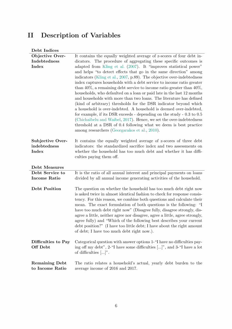
II Description of Variables

Debt Indices

Objective Over-IndebtednessIndex

It contains the equally weighted average of z-scores of four debt in-dicators. The procedure of aggregating these specific outcomes isadapted from Kling et al. (2007). It “improves statistical power”and helps “to detect effects that go in the same direction” amongindicators (Kling et al., 2007, p.89). The objective over-indebtednessindex captures households with a debt service to income ratio greaterthan 40%, a remaining debt service to income ratio greater than 40%,households, who defaulted on a loan or paid late in the last 12 monthsand households with more than two loans. The literature has defined(kind of arbitrary) thresholds for the DSR indicator beyond whicha household is over-indebted. A household is deemed over-indebted,for example, if its DSR exceeds - depending on the study - 0.3 to 0.5(Chichaibelu and Waibel, 2017). Hence, we set the over-indebtednessthreshold at a DSR of 0.4 following what we deem is best practiceamong researchers (Georgarakos et al., 2010).

Subjective Over-indebtednessIndex

It contains the equally weighted average of z-scores of three debtindicators: the standardized sacrifice index and two assessments onwhether the household has too much debt and whether it has diffi-culties paying them off.

Debt Measures

Debt Service toIncome Ratio

It is the ratio of all annual interest and principal payments on loansdivided by all annual income generating activities of the household.

Debt Position The question on whether the household has too much debt right nowis asked twice in almost identical fashion to check for response consis-tency. For this reason, we combine both questions and calculate theirmean. The exact formulation of both questions is the following: “Ihave too much debt right now” (Disagree fully, disagree strongly, dis-agree a little, neither agree nor disagree, agree a little, agree strongly,agree fully) and “Which of the following best describes your currentdebt position?” (I have too little debt; I have about the right amountof debt; I have too much debt right now.).

Difficulties to PayOff Debt

Categorical question with answer options 1-“I have no difficulties pay-ing off my debt”, 2-“I have some difficulties [...]”, and 3-“I have a lotof difficulties [...]”.

Remaining Debtto Income Ratio

The ratio relates a household’s actual, yearly debt burden to theaverage income of 2016 and 2017.

6

Sacrifice Index This index is adapted by Schicks (2013), which asks for several sac-rifices households may make because they lack money. Like them,we combine these indicators into one “sacrifice index” applying poli-choric principal component analysis such that a continuous index iscreated giving more weight to more serious sacrifices people have tomake and transforming the categorical responses into a continuousmeasure (Kolenikov and Angeles, 2009; Smits and Gunther, 2017).In total, we ask respondents about ten possible sacrifices both for ashorter term (i.e. twelve months) and for a longer term (five years).Unlike Schicks (2013), we do not pose questions about the accept-ability of sacrifices made but ask only for the frequency of distressevents that occurred in the household. We added two questions in-troduced by Smits and Gunther (2017) and two new questions thatare more context-specific to the rural setting in North-East Thai-land. Depending on the question asked, respondents could answeron a scale from 1-3 (e.g. had to work much more, more, not more)or from 1-5 (e.g. had to buy less food: never, sometimes, regularly,often, almost always, always).

Forecast Errors

QuantitativeForecast Error

Relative change between expected median income from the proba-bilistic expectations elicitation and the actual income in 2017.

QualitativeForecast Error

Difference between expected income in 2016 and actual welfare of thehousehold as evaluated in 2017.

ExpectationMeasures

Actual welfare ofthe household

Answer to “Do you think your household is better off than last year?”,from 1-“much worse off” to 5-“much better off”.

Certainty Answer to “How certain are you that this income development willtruly become reality?”. The scale ranges from 1-“Very uncertain” to4 “Very certain”.

Expected income Answer to “How do you think your average monthly income willdevelop in the next twelve months?”, from 1-“Decrease a lot” to 5-“Increase a lot”.

Probabilisticexpectations

Probabilities assessing how individuals assess future outcomes.

7

ExperimentMeasures

Treatment 1=Hard Quiz, 2=Easy Quiz.

Expected Rank Rank that participant expects to reach after taking the test quizfrom 1-“Least questions answered correctly” to 10-“Most questionsanswered correctly”.

Number of Goods Amount of goods participant wants to buy.

Overconfidence Difference between expected and actual rank of participant.

Overborrowing Dummy variable, that takes the value 1 if participant wants to buymore than earnings including endowment can pay for.

Overspending Dummy variable, that takes the value 1 if participant wants to buymore than earnings excluding endowment can pay for.

Controls

Age Age of respondent in years.

Age Squared Squared term of age.

BMI Respondent’s Body Mass Index as of 2017.

FinancialDecision Maker

Answer to question “Who is responsible for making day-to-day de-cisions about money in your household?” where means 1-“Myself”,2-“Myself and someone else” and 3-“Someone else”.

Financial LiteracyScore

Our index is based on seven questions eliciting financial knowledge,on nine assessments concerning financial behavior, and on three ques-tions regarding financial attitude. The overall index is composed ofthe sum of the sub indices and ranges between 0 and 22 with highernumbers indicating a higher level of financial literacy.

Financial RiskTaking

Answer to “Attitudes towards risk change in different situations.When thinking about investing and borrowing are you a person who isfully prepared to take risk or do you try and avoid taking risk?”, from1-“Fully unwilling to take risks” to 7-“Fully willing to take risks”.

Health Status Health status of the respondent in 2017: 1-“Good”, 2-“Can manage”,3-“Sick”

8

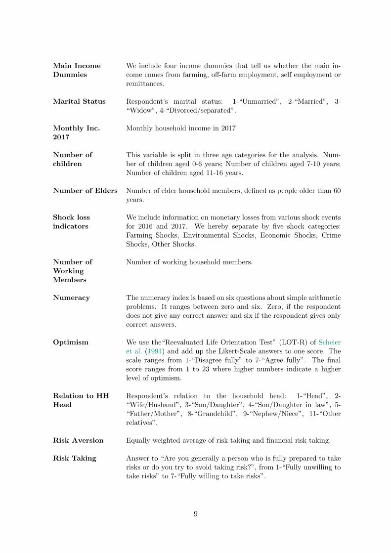
Main IncomeDummies

We include four income dummies that tell us whether the main in-come comes from farming, off-farm employment, self employment orremittances.

Marital Status Respondent’s marital status: 1-“Unmarried”, 2-“Married”, 3-“Widow”, 4-“Divorced/separated”.

Monthly Inc.2017

Monthly household income in 2017

Number ofchildren

This variable is split in three age categories for the analysis. Num-ber of children aged 0-6 years; Number of children aged 7-10 years;Number of children aged 11-16 years.

Number of Elders Number of elder household members, defined as people older than 60years.

Shock lossindicators

We include information on monetary losses from various shock eventsfor 2016 and 2017. We hereby separate by five shock categories:Farming Shocks, Environmental Shocks, Economic Shocks, CrimeShocks, Other Shocks.

Number ofWorkingMembers

Number of working household members.

Numeracy The numeracy index is based on six questions about simple arithmeticproblems. It ranges between zero and six. Zero, if the respondentdoes not give any correct answer and six if the respondent gives onlycorrect answers.

Optimism We use the“Reevaluated Life Orientation Test” (LOT-R) of Scheieret al. (1994) and add up the Likert-Scale answers to one score. Thescale ranges from 1-“Disagree fully” to 7-“Agree fully”. The finalscore ranges from 1 to 23 where higher numbers indicate a higherlevel of optimism.

Relation to HHHead

Respondent’s relation to the household head: 1-“Head”, 2-“Wife/Husband”, 3-“Son/Daughter”, 4-“Son/Daughter in law”, 5-“Father/Mother”, 8-“Grandchild”, 9-“Nephew/Niece”, 11-“Otherrelatives”.

Risk Aversion Equally weighted average of risk taking and financial risk taking.

Risk Taking Answer to “Are you generally a person who is fully prepared to takerisks or do you try to avoid taking risk?”, from 1-“Fully unwilling totake risks” to 7-“Fully willing to take risks”.

9

Self-Control We use the questions introduced by Tangney et al. (2004) and addup the Likert-Scale answers to one score. The scale ranges from 1-“Disagree fully” to 7-“Agree fully”. The final score ranges from 0 to49 where lower numbers indicate a higher level of self-control.

Sex Sex of respondent: 1-“Male”, 2-“Female”.

Total HHEducation

Sum of years all working household members went to school.

Years ofSchooling

Years respondent went to school.

Big Five -Personality Traits

Agreeableness A person, who scores high on Agreeableness (Item scale ranges from1 to 7 for all items) has a forgiving nature, is considerate and kindand not rude to others.

Conscientiousness A person, who scores high on Conscientiousnes does a thorough job,works efficiently and is not lazy.

Extraversion A person, who scores high on Extraversion is communicative,talkative, outgoing and not reserved.

Neuroticism A person, who scores high on Neuroticism worries a lot, gets nervouseasily and is not relaxed.

Openness A person, who scores high on Openness values artistic experiences, isoriginal and has an active imagination.

AdditionalControlsExperiment

Difficulties inGame

Answer to “Did the respondent have difficulties answering ques-tions?” with 1-“Not at all”, 2-“Yes, a little bit”, 3-“Yes, very much”.Filled in by the enumerator.

Morning Dummy variable that takes the value 1 if the interview took place inthe morning, i.e. before 11am.

Midday Dummy variable that takes the value 1 if the interview took placearound noon, i.e. between 12am and 2pm.

Read Alone Dummy variable that takes the value 1 if the participant could readthe experimental instructions without help. Filled in by the enumer-ator.

10

III Experimental Material

Material II.i: Instructions Experiment

Read out:

I want you to ask some test question to check whether the procedure of the ranking is clear to you. If not, I will explain it again.

After you answered this first set of questions, you have to decide how many goods you want to buy. The 40 THB that are already in your account are given you as a credit that you can use to buy the goods. With the money you earn in the second round in the quiz you will pay back your credit. If you spend more money than you earned we will keep the money from your account and give you the goods you have bought. If you earned more than you bought, you pay back your credit and can keep the rest of the money and goods.

[Hand respondent the first quiz (green paper). If respondent cannot read, assist in all tasks]

If you don’t have any further questions we start with the first round. [FAQ]

In the first round, you will get 7 test questions, which are very similar to the questions you will get in the second round. But again, you can ONLY earn money in the second round.

[Show picture of ranks, payoffs and people]

Test Question 1: What does it mean to be ranked 6? [Open answer; enumerator please continue if you think the respondent gave a correct answer]

Test Question 2: How much money do you earn if you are ranked 6? [Answer: 10 THB]

Test Question 3: How many goods you can buy for 10 THB? [Answer: 1]

The money you earn, will be put on your game account which already has 40 THB in it. As you can see from the picture, you can earn up to additional 40 THB. The quiz for which you will receive money will be played in the second round.

Experiment Script

We want to play a market game with you. In this game you can earn money and buy goods. The kind of goods you can buy are placed right next to you. Each piece has a value of 20 THB, but we offer them to you for a discounted price of 10 THB. You don’t have to buy one kind of product, but can buy different kinds (for example 2 chocolate bars and 1 bag of chips). If you don’t like to buy anything you can keep the money you earn.

To earn money, you have to play a quiz which consists of 15 questions. 10 persons from another village, which is similar to your village, took the same quiz before. The amount of money you earn is dependent on how many questions you answered right in comparison to these villagers. In this picture, the person who has given the most correct answers is ranked 10, the person who has given the second most correct answers is ranked 9, the person who has given the third most correct answers is ranked 8, and so on. In the picture you can also see how much money you will earn dependent on your ranking. For example, if you are ranked 7 you will earn 20 THB. Please take your time to understand how you can earn money in this game.

11

[Please note which goods were finally kept]

Thank you very much for your participation, we hope you enjoyed the game. I will now calculate your earnings and inform my STL which will bring you your payment and goods.

Question 3 [Only ask if expected earning of respondent was more than 0 THB]: Would you have buy less goods, if you thought your earnings would be lower?

[Calculate rank, earnings and cash/goods payoff. Wait for STL to hand the money/goods]

{In the very unlikely case, that more goods were wanted than earnings are generated:}

I calculated your earnings and you cannot afford all the goods you want to buy. You want to buy […] goods but can only afford […] goods. Please, choose which goods you want to keep.

[Hand the second quiz, set your alarm clock to 10 minutes and tell respondent to start]

The time is up. Please, hand me the second quiz. Before we conclude, I have some final questions for you.

Question 1: After taking the quiz, when 1 is the villager who gave the least correct answers and 10 is the villager who gave the most correct answers, where do you see yourself in this picture?

Question 2 [Only ask if expected earning of respondent was smaller than 40 THB]: Would you have buy more goods, if you thought your earnings would be higher?

[Set your alarm clock to 5 minutes and tell the respondent to start]

The 5 minutes are over. Please, stop answering the test quiz and make your decisions on the white sheet of paper. Give me a sign when you have made your decisions, then I will collect the white paper.

[During the time the respondent takes the second quiz, evaluate the white sheet of paper and enter the numbers on the tablet]

Now, in the second round, you play the quiz that decides how much money you earn. You have 10 minutes to answer the questions. Afterwards, I will collect the quiz, calculate your earnings and hand you the goods and money.

Please read through the questions on the green sheet of paper and try to answer as many questions as you can. You have 5 minutes to answer the questions. I will tell you when the 5 minutes are over. After you have finished the quiz, please have a look on the white piece of paper and answer these questions and make your buying decision. When you have finished the first round, I will collect the white piece of paper. You can keep the green paper with the test quiz. It is only for you, so that you know what kind of questions to expect in the quiz of the second round.

12

Material II.ii: Guideline for Interviewers to Answer Questions from Participants

Frequently Asked Questions

Respondent: “What if I don’t want to buy anything?”You: “You don’t have to buy anything, you can also keep the money.”

Respondent: “Can I spend all my money on buying products?”You: “Yes you can, but if you do not earn enough money to pay all the products you wanted tobuy, you will only get the part of the products you can afford.”

Respondent: “Can I change my buying decision after I took the second quiz?”You: “No, your decision is fixed. Only in the case where you wanted to buy more products thanyou have money available, you can decide on which products to keep”

Respondent: “What happens if I spend more money on products than I earn?”You: “Then we will take the money from the 40 THB that are already on your virtual bankaccount for the game. If even this is not enough, you only get as many products as you havemoney. We will NOT take any out of your pocket and we will NOT take money from the 50 THByou get for the questionnaire. We only count the money you get in the game.”

Respondent: “Does being on rank 7 means that I need to get 7 questions correct?”You: “No! It means that three persons have answered more questions correctly than you and sixpersons have answered less questions correctly than you. The rank is always dependent on howmany questions you have correct in comparison to the other 10 villagers. In this case you are asgood as the villager who was ranked 7.”

Respondent: “Does it make a difference which questions I answer correctly?”You: “No, all questions count the same.”

Respondent: “Do the products really cost 20 THB per piece?”You: “Yes, if you buy them as presented here, they cost 20 THB.”

[Respondent: “What if I don’t know the answer to a question at all?”You: “Just take a guess. You don’t receive some sort of minus points for wrong answers.”]

Respondent: “What if I cannot finish the quiz in time?”You: “That is no problem. Please, try to answer as many questions as you can in the given timeframe. There will be no minus points for unanswered questions.”

Respondent: “Who are the other 10 persons who have answered the quiz before?”You: “They are just some randomly selected persons from another village, that is similar to yourvillage.”

13

Material II.iii: Quiz-Hard Treatment

Ottawa O positive

Vancouver AB positive

Montreal B positive

Toronto A positive

Chicken Pineapple

Duck Mango

Penguin Banana

Squirrel Passion Fruit

144 Leo

94 Pisces

88 Dragon

126 Scorpio

Hokkaido and Kyushu

Shikoku and Hashima

Okinawa and Okinoshima

Hiroshima and Nagasaki

2. What is the most common blood type in the world?

7. Which are the Japanese cities that were hit by atomic bombs of the U.S. army during WWII?

5. How many days does Mercury need to orbit the sun?

3. Which animal cannot fly? 4. Which fruit contains the most amount of Vitamin C per 100g?

6. Which animal is not part of the Zodiac?

1. What is the biggest city in Canada by population?

Test Quiz

14

Tiger Euro

Eagle US. Dollar

Lion Pound

Panda Deutsche Mark

47 provinces Grasshopper

48 provinces Spider

49 provinces Beetle

50 provinces Centipede

Austria Coca Cola

France Beer

Sweden Tea

Poland

Italy Lungs

France Heart

Spain Liver

Portugal Brain

5. Which of these countries does NOT border Germany?

6. Which is the most drank beverage in the world?

Coffee

1. What is the national animal of China?

7. Which country is the origin of pizza?

8. Which of these four is the biggest organ of the human body?

Quiz

2. If Thai currency is THB, what is the currency of Germany?

3. How many provinces does Japan have currently?

4. Which is the heaviest insect in the world?

15

Susilo Bambang Yudhoyono Red

Joko Widodo Gold

Abdurrahman Wahid Green

Megawati Sukarnoputri Pink

Black, Blue and Gold Blueberry

Black, Red and White Pear

Black, Red and Gold Apple

Black, Red and Blue Kiwi

Grey

Dark green

Black

Brown 2 seasons including rainy and winter

Nabi Muhammad

Yahweh

Allah

Moses QID:

3 seasons including rainy, winter and spring

2 seasons including summer and winter15. Who is the God of Islam?

10. What color is traditionally not associated with Christmas Day?

13. What color will you get if you mix blue, red and yellow?

14. How many seasons are there in Germany? And which ones?

11. Of which colors is the flag of Germany composed of?

12. Which fruit is blue?

4 seasons including spring, summer, autumn and winter.

9. Who is the president of Indonesia?

16

Material II.iv: Quiz-Easy Treatment

Ubon Ratchathani Grey

Chiang Mai Green

Bangkok White

Surat Thani Pink

Asian Buffalo Banana

Dog Papaya

Elephant Durian

Tiger Apple

Vietnam Monkey

Laos Horse

Cambodia Cat

Myanmar Dragon

Blue

Brown

Green

Hazel

3. Which animal cannot jump? 4. Which fruit is prohibited in public transport around South-East Asia?

6. Which animal is not part of the Chinese Zodiac?

Test Quiz

5. Which of these countries does NOT border Thailand?

2. What color will you get if you mix blue and yellow?

7. What is the most common eye color in the world?

1. What is the biggest city in Thailand?

17

Elephant Euro

Eagle US Dollar

Lion Pound

Naga (Thai Dragon) Franc

76 provinces Blue Shark

77 provinces Killer Whale

78 provinces Blue Whale

79 provinces Elephant

6 3 seasons including summer, rainy and winter

5 2 seasons including summer and rainy

4 2 seasons including rainy and winter

7

Coconut Milk Skin

Tomatoes Eyes

Oyster Sauce Mouth

Chili Paste Ears

5. How many months have 31 days?

6. How many seasons are there in Thailand? And which ones?

4 seasons including summer, rainy, autumn and winter

1. What is the national animal of Thailand?

7. Which of these do you need to make traditional Som Tam Thai?

8. Which is the biggest sense organ of the human body?

Quiz

2. If Thai currency is THB, what is the currency of USA?

3. How many provinces does Thailand have currently?

4. Which is the biggest animal in the world?

18

Donald Trump Red

Barack Obama Pink

Angela Merkel Green

Bill Clinton Light blue

Green, White and Red Durian

Green, White and Blue Jackfruit

Blue, White and Red Rambutan

Blue, Red and Yellow Salak

4th Reign Thailan

5th Reign

6th Reign Cambodia

7th Reign

Nabi Muhammad

Jesus

Guanyin

Vishu QID:

China

15. Who is the son of god of Christianity?

10. What is the color of the day on Wednesday?

13. Which reign of Thailand abolished slavery?

Germany

14. Which country has the highest total rice consumption?

11. Of which colors is the flag of Thailand composed of?

12. Which fruit does not have thorns?

9. Who is currently the president of the United States of America?

19

Material II.v: Decision Sheet

Question 2: We told you that the money you will earn in the secondquiz depends on how you actually are ranked in this picture above. Forexample if you are ranked 7, which means that 3 villagers gave morecorrect answers than you and 6 villagers gave less correct answersthan you, you will get 20 THB. What do you think, how much moneywill you earn?

7

฿

Before you take the second quiz where you can earn money, we havesome questions for you and you have to decide which goods and howmany you want to buy.

8 9 100 ฿ 10 ฿ 20 ฿ 40 ฿

1 2 3 4 5 6

Question 1: As mentioned before, 10 persons from another villagetook the same quiz as you will have to take now. After taking the testquiz and knowing the second quiz will be similar: When the villager onthe left side of this picture is the one who gave the least correctanswers and the villager on the right side of this picture is the onewho gave the most correct answers, where do you see yourself in thispicture? Please cross the respective box.

20

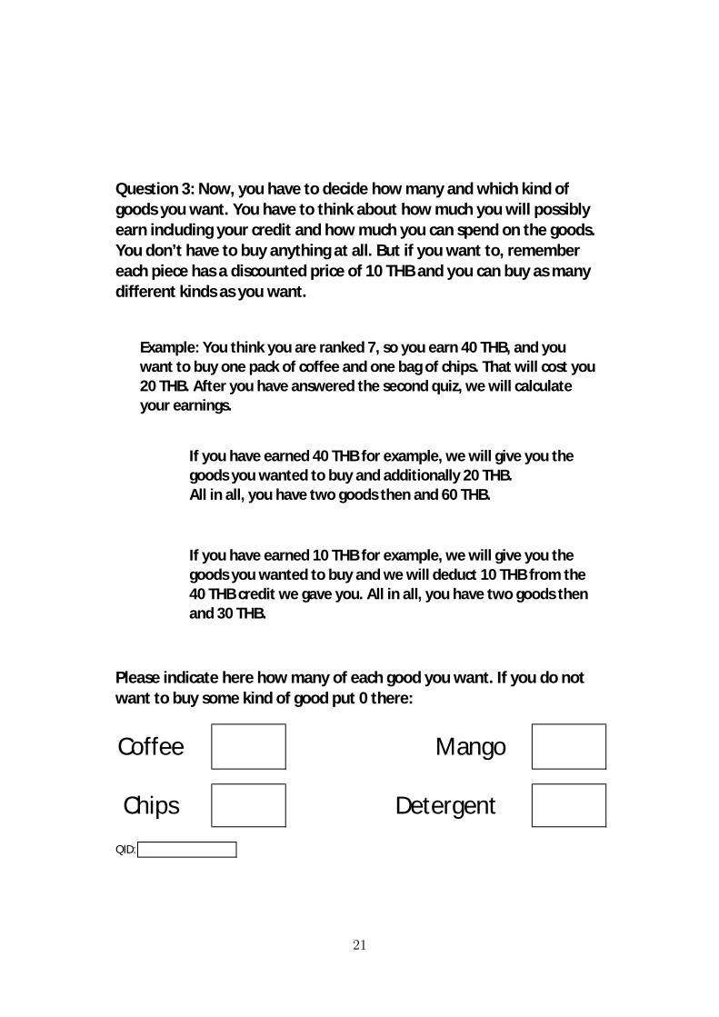
Detergent

QID:

MangoCoffee

Chips

If you have earned 10 THB for example, we will give you thegoods you wanted to buy and we will deduct 10 THB from the40 THB credit we gave you. All in all, you have two goods thenand 30 THB.

Please indicate here how many of each good you want. If you do notwant to buy some kind of good put 0 there:

Example: You think you are ranked 7, so you earn 40 THB, and youwant to buy one pack of coffee and one bag of chips. That will cost you20 THB. After you have answered the second quiz, we will calculateyour earnings.

If you have earned 40 THB for example, we will give you thegoods you wanted to buy and additionally 20 THB.All in all, you have two goods then and 60 THB.

Question 3: Now, you have to decide how many and which kind ofgoods you want. You have to think about how much you will possiblyearn including your credit and how much you can spend on the goods.You don’t have to buy anything at all. But if you want to, remembereach piece has a discounted price of 10 THB and you can buy as manydifferent kinds as you want.

21

don’t expect too much - high income expectations and over

Documents