donald uncertainty qmra

8/12/2019 Donald Uncertainty QMRA

http://slidepdf.com/reader/full/donald-uncertainty-qmra 1/17

Incorporating parameter uncertainty into Quantitative

Microbial Risk Assessment (QMRA)

Margaret Donald, Kerrie Mengersen, Simon Toze, Jatinder P.S. Sidhu

and Angus Cook

ABSTRACT

Modern statistical models and computational methods can now incorporate uncertainty of

the parameters used in Quantitative Microbial Risk Assessments (QMRA). Many QMRAs use

Monte Carlo methods, but work from fixed estimates for means, variances and other parameters.

We illustrate the ease of estimating all parameters contemporaneously with the risk assessment,

incorporating all the parameter uncertainty arising from the experiments from which theseparameters are estimated. A Bayesian approach is adopted, using Markov Chain Monte Carlo

Gibbs sampling (MCMC) via the freely available software, WinBUGS. The method and its ease of

implementation are illustrated by a case study that involves incorporating three disparate datasets

into an MCMC framework. The probabilities of infection when the uncertainty associated with

parameter estimation is incorporated into a QMRA are shown to be considerably more variable

over various dose ranges than the analogous probabilities obtained when constants from the

literature are simply ‘plugged’ in as is done in most QMRAs. Neglecting these sources of

uncertainty may lead to erroneous decisions for public health and risk management.

Key words 9999 MCMC, parameter uncertainty, Quantitative Microbial Risk Assessment (QMRA)

recycled water, risk assessment, Salmonella spp.

INTRODUCTION

In Australia, Quantitative Microbial Risk Assessment

(QMRA) is recommended as the method of choice for asses-

sing health risks from exposure to pathogens in recycled

water, e.g. NRMMC (2006). The particular application exam-

ined in this paper is the risk of microbial infections associatedwith exposure to recycled water.

This paper presents a modification to the standard

QMRA methodology, in which the risk assessor typically

finds various quantities of interest, such as dose–response,

die-off and/or log-reduction parameters and plugs these

quantities into the risk assessment model. There is often little

acknowledgement of the fact that these quantities are uncer-

tain. We contrast this ‘plug-in’ approach with an approach

based on a Bayesian risk assessment model, in which all the

data which have been used to produce the quantities of

interest necessary to the risk assessment are included. Theuncertainty associated with the model parameters is therefore

propagated throughout the analysis. This may be considered

an extension of the standard QMRA model.

To illustrate the approach, we consider the probability of

a person becoming infected with Salmonella spp. after being

exposed to recycled wastewater. The scenario is not drawn

Margaret Donald (corresponding author)

Kerrie Mengersen

Queensland University of Technology,

George Street,

Brisbane, QLD 4000,

Australia

Tel.: þ 617 3138 1292

E-mail: [email protected]

Simon Toze

Jatinder P.S. Sidhu

CSIRO Land and Water,

Queensland Biosciences Precinct,

306 Carmody Road,

St Lucia, QLD 4067,

Australia

Simon Toze

School of Population Health,

University of Queensland,

Herston Road,

Herston,

Brisbane, QLD 4006,

Australia

Angus Cook

School of Population Health,

University of Western Australia,

35 Stirling Highway,

Crawley, WA 6009,Australia

doi: 10.2166/wh.2010.073

10 & Queensland University of Technology 2011 Journal of Water and Health 9999 09.1 9999 2011



from actuality but is designed to illustrate the extension of the

standard QMRA methodology. In the illustration, we ignore

the problems of dose estimation, and investigate the part of

risk estimation for which we have data available.

This paper is arranged as follows. First a standard QMRA

method is outlined, followed by a brief description of the

extended method, together with the datasets which will be

used to illustrate it. The conceptual and statistical models into

which these data are incorporated are then detailed, and the

results are compared with those one would obtain without

the incorporation of parameter uncertainty. This case study

demonstrates that considerable uncertainty is induced in the

probability of infection when this Bayesian approach is

adopted. In the discussion, we elaborate the differences

seen between the two methods and note the simplicity of

our method.

METHODS

Standard QMRA methodology

A QMRA requires a knowledge of pathogen numbers at some

stage of the treatment process, generally in the influent.

Estimates for log reductions for various water treatment

processes from pilot or other studies are then needed toestimate pathogen numbers in the treated water. A mechan-

ism of ingestion and an amount of the treated recycled water

ingested must be postulated or found. This, together with the

pathogen numbers in the treated water, allows estimation of

possible microbial doses. Finally, specification of a dose–

response curve for the microbe of interest is needed to

allow estimation of the probability of infection given a

particular dose. A natural representation for a QMRA is via

a graphical model such as Figure 1.

The QMRA of Figure 1 shows the steps for assessing the

risk associated with eating a crop irrigated with recycled water.

In such a figure, nodes without parents need information

in order to run the risk assessment. Thus, for a standard

QMRA, reading down the figure and from left to right, we

need:

1. A description of the microbe numbers in either the waste-

water or in the final treated water. Typically, if Salmonella

spp. is sampled at all, it is sampled in the wastewater and

may be described as coming from a log normal distribution

with mean, m, and possibly a standard deviation s.

2. ‘Log reductions’ in order to estimate the microbial num-

bers in the treated water. Water treatments are generally

thought to reduce the numbers of pathogens at a rate

proportional to the influent numbers of the pathogen in

the water. This may be expressed in terms of log base 10,

when it may be referred to as ‘log reduction’ or a decimal

elimination capacity (DEC); see, for example, Hijnen et al.

(2004, 2007). However, the DEC is typically given by a

single number, e.g. 3, which would mean that log10C influent -

log10C effluent ¼ 3, where C influent is the number/L in the

influent and C effluent is the number/L in the effluent. Such a

log reduction would imply that the effluent numbers are

Figure 1 9999 Model for a QMRA for surface vegetable irrigated with treated wastewater.

Observed data nodes shown in white, parameter nodes in dark grey and

outcome nodes in a lighter shade of grey.

11 M. Donald et al . 9999 Incorporating parameter uncertainty into QMRA Journal of Water and Health 9999 09.1 9999 2011



one thousandth those of the influent. To find these, pub-

lished or grey literature involving the particular treatment

type for a particular plant is searched.

3. A die-off constant k or T 90 (time to 90% die-off). In the

case study, where a field is irrigated with recycled waste-

water, it is expected that sunlight will kill particular

microbes at a rate proportional to their number, i.e.

d N /dt p N or N t ¼ N 0e-kt , where k is sometimes referred

to as the die-off constant. Other equations may be used,

but this is a reasonably common approximation to die-off

for some organisms, and is a good fit for the data used in

this case study. Sinton et al. (2007) use a ‘shoulder’

equation (100[1[1exp(kT )]n]), but, as is common,

the quantities in their various equations are given as

constants, with no error indicated.

4. Sunlight and shade hours, for the locality in which the

recycled water is to be used.

5. A suitable amount of crop/water ingested by a person. One

may use survey data if available, or use choices made by

other researchers, for example, Tanaka et al. (1998). (Typi-

cally such data are supplied as constants.)

6. An equation and the parameters which describe the dose–

response, i.e. the probability of becoming infected, having

ingested a particular dose of the microbe. For Salmonella,

the equation usually used is beta-Poisson, and from p 401

of Haas et al. (1999), the risk assessor would select

a¼ 0.3126 and N 50 ¼ 2.36 104, to give the probability of

infection, P , from a given dose D, where D is the number

of microbes ingested, as: P ¼ 1[1 þ ( D/ N 50)(21/a1)]a.

In an alternative parameterization, we have P ¼ 1[1 þ

( D/b)]a, where b ¼ N 50(21/a1)D193 120, and N 50 is the

number of microbes which give a 50% probability of

infection.

Thus, to perform a risk assessment, the risk assessor

performs a Monte Carlo simulation, working through the

graphical model (Figure 1). Starting at some stage in the

water processing cycle, an initial number/L of the pathogen is

drawn from the water treatment distribution described by

constants m0, s0. This number is then reduced by either the

value obtained by drawing a log-reduction value from the

DEC distribution, described by m1, s1, or, if no distribution is

given or able to be inferred, then reduced by the DEC, m1, for

the process or processes. In the scenario considered, sunlight

is expected to reduce pathogen numbers, so the die-off

equation is used to give a final pathogen number in water

which, then, together with a draw for the quantity of water

ingested, gives the number of pathogens ingested. Finally, the

probability of infection is calculated, via a dose–response

equation, and a final draw made from a Bernoulli distribution

to simulate the person’s infection status. This is repeated

many times to simulate the risk, resulting in a distribution

of the simulated endpoint risk.

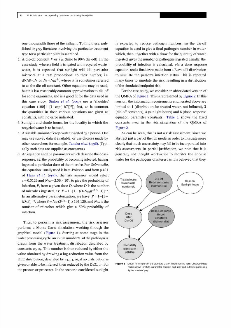
For the case study, we consider an abbreviated version of

the QMRA of Figure 1. This is represented by Figure 2. In this

version, the information requirements enumerated above are

limited to 1 (distribution for treated water, not influent), 3

(die-off constants), 4 (sunlight hours) and 6 (dose–response

equation parameter constants). Table 1 shows the fixed

constants used in the risk simulation of the QMRA of

Figure 2.

As can be seen, this is not a risk assessment, since we

abstract just a part of the full model in order to illustrate more

clearly that much uncertainty may fail to be incorporated into

risk assessments. In partial justification, we note that it is

generally not thought worthwhile to monitor the end-use

water for the pathogens of interest as it is believed that they

Figure 2 9999 Model for the part of the standard QMRA implemented here. Observed data

nodes shown in white, parameter nodes in dark grey and outcome nodes in a

lighter shade of grey.




will be present in such small quantities and will be so diffuse

within the water body that substantive positive results would

only be obtained by processing impractically large samples.

Data on pathogen reductions or log reduction studies exist

but have been collected from typically small-scale, short-run

experiments, usually in countries with very different climatic

conditions. Moreover, such data may be owned by private

utilities and are either not publicly available, or provided with

minimal details. Thus, often only summary statistics or

incomplete statistics (at best) filter into the public domain.

If the risk of a particular health outcome needs to be

estimated, available data are even more limited. For example,

Salmonella spp. have been linked with a number of outbreaks

in the USA, Europe and Japan (Marks et al. 1998). In

Australia, limited data for Salmonella spp. numbers and

their inactivation by various wastewater treatment processes

are available. The few studies available are those of Gibbs and

others, and these focus on Salmonella spp. in sludge, rather

than within the water fraction (Gibbs & Ho 1993; Gibbs 1995;

Gibbs et al. 1995).

Thus, this study takes a small part of the risk assessment

process and shows how it may be extended, by embedding

data within a Bayesian framework to estimate the corre-

sponding parameters, and thereby give better uncertainty

estimates. The extended model for doing this is described in

the next section.

The extended QMRA model

In the extended model, the small experiments which lead to

the various required constants are incorporated directly into

the risk assessment process, allowing the uncertainty asso-

ciated with the estimates to be automatically incorporated

into the risk assessment. Thus, Figure 3, the extended model,

contains two additional nodes (1 and 7) in comparison with

Figure 2, the standard QMRA. These nodes represent the data

which give rise to the ‘constants’ fed into the QMRA assess-

ment of Figure 2, but in the extended model are used to derive

estimates of the random quantities that describe these data.

The starting point for the extended model is the graphical

representation of the QMRA which is seen to be a directed

acyclic graph or DAG. Thus, a risk assessment may be

embedded in a Bayesian framework, thereby allowing para-

meters to be estimated simultaneously with the risk assess-

ment. In the extended model (Figure 3), parameters (supplied

as constants under Figure 2) are both estimated and used for

the derivation of other quantities. Thus, the model descrip-

tions at nodes (2) and (6) are the explanatory models of the

data at the new nodes (1) and (7), and also the means for

estimation of dose after die-off (node 5) and estimation of the

probability of a person becoming infected (node 8). In this

Bayesian framework ‘prior’ probabilities (prior beliefs) for the

parameters of the explanatory models are needed and unin-

formative priors are used in order that the parameter esti-

mates and the uncertainty associated with them will closely

approximate the maximum likelihood solutions for each set

of parameters and data.

As with the standard QMRA model, a Monte Carlo

approach is taken to analyse the extended model. Here,

however, given the Bayesian setup and additional informa-

tion, a more formal Markov chain Monte Carlo approach is

used to estimate posterior distributions of the various quan-

tities of interest such as dose–response parameters, die-off

parameters and the risk of infection. The Bayesian framework

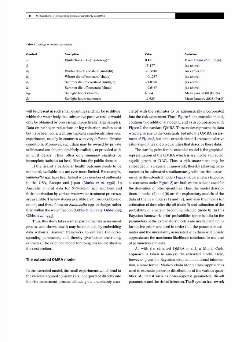
Table 1 9999 Settings for constant parameters

Constant Description Value Derivation

a P (infection) ¼ 1(1 þ dose/b)-a 0.451 From Teunis et al. (1996)

b 15 177 (as above)

k1 Winter die-off constant (sunlight) 0.3010 An earlier run

k2 Winter die-off constant (shade) 0.1237 (as above)

k3 Summer die-off constant (sunlight) 1.0390 (as above)

k4 Summer die-off constant (shade) 0.6457 (as above)

SW Sunlight hours (winter) 6.584 Mean June 2008 (Perth)

SS Sunlight hours (summer) 11.625 Mean January 2008 (Perth)




used was the freely available WinBUGS (Lunn et al. 2000).

This is described in more detail later in the context of the case

study.

We now give a more detailed description of the data and

the models used to explain them.

Data for the extended model

Three disparate sources of information are integrated into the

model described above: die-off data for S. typhimurium,

dose–response data for S. anatum (Teunis et al. 1996) and a

short run of weather data from an Australian city, Perth

(Bureau of Meteorology 2010, pers. comm), giving the number

of hours of sunlight in a summer and a winter month. We also

use a fictitious pathogen distribution for the treated water

with a range which allows the possibility of a 100% infection

rate. These datasets and distributions are now described in

more detail.

Salmonella dose-response data (Figure 3, node 7)

In considering the risks of Salmonella spp. poisoning, we

chose to use the S. anatum data presented in the report

by Teunis et al. (1996), in which infection curves were fitted

by strain and species. These authors concluded that for

S. anatum the three strains could be grouped together to

determine a single dose–response curve, using a likelihood

ratio test. Others have made different choices; thus Haas et al.

(1999) used all 13 species and strains detailed in Teunis et al.

(1996) and discarded some ‘outliers’, after similar testing, as

did Oscar (2004). Each of these authors’ strategies gives a

different set of quantities which the risk-assessor may use, but

whatever parameter estimates he/she uses, they are used

without any error being associated with them. Our purpose

was not to determine a best model for dose–response for

Salmonella, but to show how to incorporate the uncertainty

associated with the estimation of such model parameters into

a risk assessment.

A further reason for using Salmonella dose–response data

is that the data are best summarised by a beta-Poisson dose–

response curve, where the probability of infection for a given

dose of D microbes, is given as P (infection) ¼ 1(1 þ D/b)a,

which is characterised by two parameters (a, b) which are

highly correlated.

Hence, there are two issues here in using these para-

meters in a risk assessment. Firstly, they are typically included

as point estimates without acknowledgment of uncertainty of

specification or of their correlation. However, even if this

uncertainty were included, it is preferable to use the posterior

distribution of the two parameters directly instead of making

the standard assumption of bivariate normality, which Teunis

et al. (1996) have shown does not hold.

Figure 3 9999 Schematic model for the directed acyclic graph implemented in WinBUGS for estimation of parameters and risk. Observed data nodes (1, 3, 4, 7) are shown in white. Unknown

parameter nodes to be estimated (2, 6) are in dark grey and outcome nodes (5, 8) are in a lighter shade of grey.




Salmonella typhimurium die-off data (Figure 3, node 1)

Salmonella typhimurium die-off data from Sidhu et al. (2008)

were supplied by the authors. These data allow the estimation

of die-off rates with uncertainty for S. typhimurium under

several conditions, winter/summer, sun/shade and grass/

thatch. The available dataset consists of 34 observations.

The summer observations were taken over all the combina-

tions of conditions, but the winter data were for grass only

and measured die-off in light and shade, thereby giving six

sets of experimental conditions, and potentially six die-off

constants. In the experiment, grass irrigated with sterile

effluent was seeded with known numbers of S. typhimurium

and samples of the grass and thatch were then harvested at

1, 2, 4, 6, 7.3 and 9.3 h after the initial seeding (in summer).

Microbial numbers were counted and averaged for the sam-

ples taken at each harvest time and sample type (sun/shade,

grass/thatch). For the winter samples, harvest times were 1, 2,

4, 6, and 8 h and grass and thatch were not separated. For

further details of the experiment, see Sidhu et al. (2008).

Die-off over time is expected to be proportional to the

number of organisms. Thus, d N /dt p N . This equation has the

solution N t ¼ N 0ekt , where k is positive. One can use any base

for exponentiation and this changes the constant, k, often

referred to as the ‘die-off’ constant. To avoid confusion about

bases for exponentiation, the constant used to express this

equation may be given as T 90 or the time to 90% die-off. Solving

0.10 ¼ exp(kT 90) gives T 90 in terms of k and vice versa.

Microbial count numbers are usually thought to be log

normally distributed. Hence, the die-off distribution equation

takes the form log(Nt)B N (log(N0) kt, s2) or, alternatively,

log( N t / N 0)B N (kt , s2). We fit the second version of this

equation for each set of experimental conditions. This was

done because greater effort (in terms of replicates) had gone

into finding the value of the initial seedings. The original

complete data had shown differences in the die-off rates for

all combinations of sun/shade and winter/summer, but none

for thatch. Hence, we fit four die-off constants, k1,y,k4 to the

model log( N i,t / N i,0)B N (kit , s2), where i references the

summer/winter, sun/shade combination, and a common

(pooled) variance s2 is used. Natural logs were used and

the die-off value was not constrained to be negative; indeed,

14% of the posterior estimates for die-off in winter and in the

shade were positive. When this occurred, a zero was sub-

stituted in the corresponding decay equation in the risk

modelling (see below), although some evidence exists for

the regrowth of Salmonella spp. on lettuce leaves under the

right circumstances (Brandl & Amundson 2008).

The posterior estimates for die-off act on the treated water

pathogen number node (node 3 of Figure 3), together with the

sunlight hours of node 4, to produce the dose after die-off at

node 5. The die-off calculation uses the maximum 17 h

period for winter and summer available for die-off, based

on the irrigation regime for the sports ovals in Perth where

the experimental die-off data were collected. Note that the

various values of k are the die-off constants of item 3 in the

description of standard QMRA methodology.

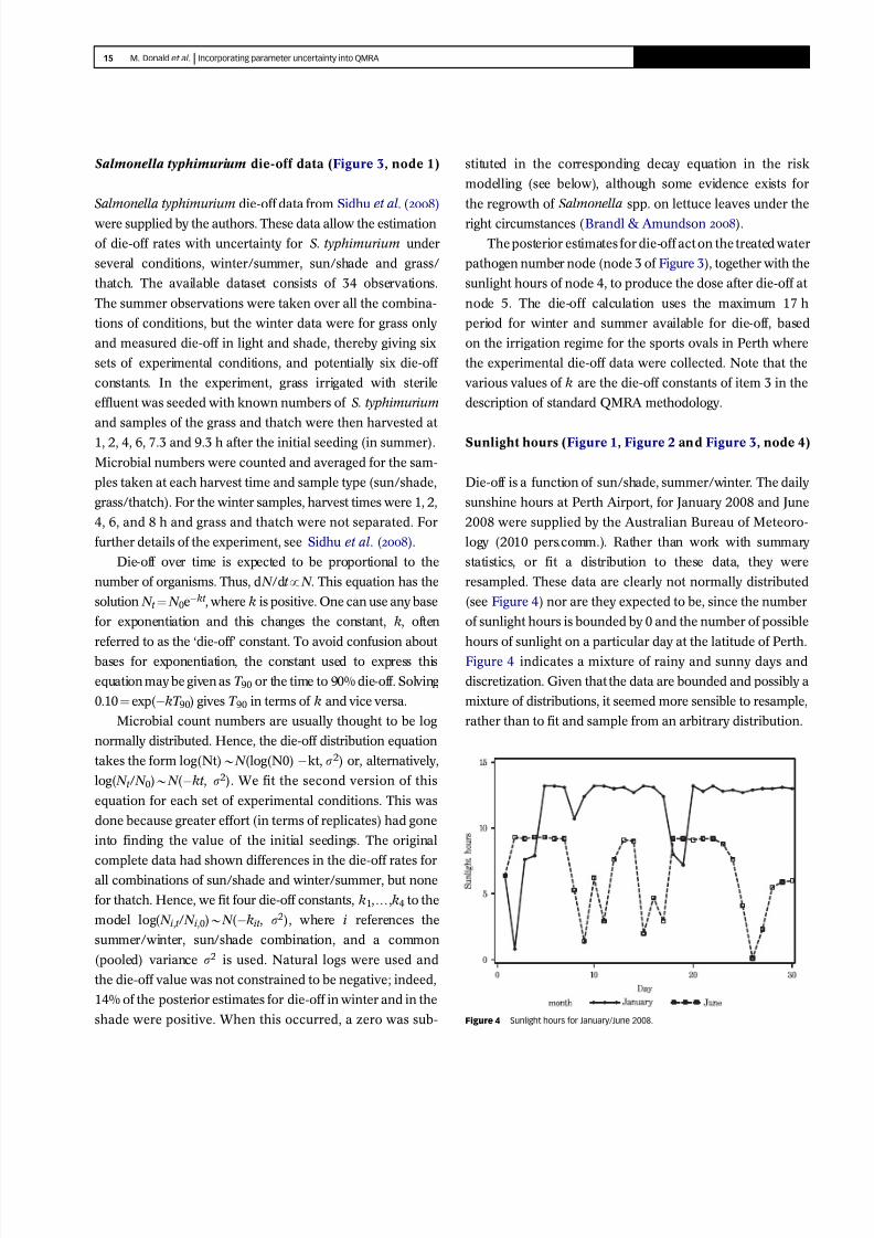
Sunlight hours (Figure 1, Figure 2 and Figure 3, node 4)

Die-off is a function of sun/shade, summer/winter. The daily

sunshine hours at Perth Airport, for January 2008 and June

2008 were supplied by the Australian Bureau of Meteoro-

logy (2010 pers.comm.). Rather than work with summary

statistics, or fit a distribution to these data, they were

resampled. These data are clearly not normally distributed

(see Figure 4) nor are they expected to be, since the number

of sunlight hours is bounded by 0 and the number of possible

hours of sunlight on a particular day at the latitude of Perth.

Figure 4 indicates a mixture of rainy and sunny days and

discretization. Given that the data are bounded and possibly a

mixture of distributions, it seemed more sensible to resample,

rather than to fit and sample from an arbitrary distribution.

Figure 4 9999 Sunlight hours for January/June 2008.




Doses (item 5, standard QMRA methodology sectionand Figure 1)

No data were used for the person’s dose. This node is not

included in the case study (Figures 2 and 3).

The Salmonella dose–response curve (Figure 5) shows

that very high doses of S. anatum are required for infection.

(Using the point estimates found by Teunis et al. (1996), a

dose of 400 S. anatum gives a probability of infection of 0.01,

while for a dose of 1000 the probability of infection becomes

0.03.) Given the probabilities of infection, it appears that the

dose–response curve applies largely to healthy adults. Since

small children and the elderly are more likely to become ill

under the same dosing regime, a range of doses was induced

(via the treated water pathogen numbers distribution) in

order to see the effect of parameter uncertainty over the full

dose–response curve.

Under the models used in this case study, the node

‘person’s microbe dose’ of Figure 1 is equated to ‘dose after

die-off’ (Figure 2 and node 5 of Figure 3).

Treated water numbers

This node is a derived node in Figure 1 but an initial node in

Figures 2 and 3. The pathogen numbers’ distribution in

treated water was ascribed a (natural) log-uniform distri-

bution over the range (-1, 30). Thus, in this study, both

consumption rates and numbers per L of the pathogen

in the recycled or the influent source water were igno-

red. Instead, an arbitrary distribution was chosen for the

Salmonella spp. numbers distribution in treated water, to

allow the possibility of seeing the effect of the uncertainty

in die-off rates and the uncertainty in the dose–response

parameters on the estimate of the probability of infection,

under many possible scenarios.

Putting it all together

Conceptual model

The directed acyclic graph for the extended model (the

‘conceptual model’) is given by Figure 3. Here, the Sidhu

et al. (2008) data (node 1) are explained by the regression

model (Equation (3)) of node 2 which estimates the die-off

parameters. For each iteration of the MCMC algorithm, the

four die-off rates are estimated; a dose sample is drawn from

node 3; and a sample is drawn from the sunlight hour data of

node 4. At node 5, the die-off constants for this iteration are

applied using Equations (4)–(8) for a 17 h day with the

sunlight and shade hours from node 4. When the draw for

the winter shade or sunlight die-off parameter is negative, it is

replaced by zero.

Independently, the Teunis etal. (1996) dose–response data

for S. anatum(node 7) areexplained by thecurrent estimates of

(a,b) (node6, and fitted using Equations (1) and (2)), which are

used in the same MCMC iteration (at node 8, using Equations

(9) and (10)) to calculate the probability of infection,

thus allowing a single estimate of the probability of infection

(and the infection status of an individual) at each iteration.

Statistical model

Node 7 contains the dose–response data from Teunis et al.

(1996) which may be represented as ( Di, N i, X i), i ¼ 1,y,19,

where Di is the ith dose, N i is the number of subjects given the

ith dose and X i is the number of subjects infected by the ith

dose.

These are explained by the dose–response equation (node

6, Equations (1) and (2)) with parameters (a, b). Uninforma-

tive log-uniform priors are given for (a, b), and after burn-

in, the posteriors for (a, b) are essentially identical to theFigure 5 9999 Dose–response curve with uncertainty for S. anatum: P ¼ 1-(1 þ Dose/b)-a. The

bounding curves are the 95\% credible intervals from the MCMC simulation.




maximum likelihood estimates. Thus, nodes 6 and 7 are

described by

X iBBinð pi; N iÞ ð1Þ

pi ¼ 1 1 þ Di

b

a

: ð2Þ

with priors for (a, b) given by

lnðaÞBU ð10; 15Þ

lnðbÞBU ð6; 20Þ:

The current MCMC simulation of the posteriors for (a, b)

is passed to node 8, again using Equations (1) and (2) (but

now in the form of (9) and (10)), to give a value for the

probability of infection (and whether an individual is

infected) after sunlight die-off.

Node 1 represents the die-off data, which may be con-

sidered as (L j, t j, N 0( j), N t ( j)), j ¼ 1,y,34. j references each data

point, while L j ¼ 1,y,6, represents the line and experimental

condition to which the jth point belongs, and there are 6 of

these corresponding to the number of different conditions of

the experiment, t j is the number of hours elapsed from the

initial seeding (with count N 0( j) on line L j) and N t ( j) is the

count at time t j for line L j. The die-off constants kL( j) ¼ kl,L j ¼ 1,y,6, j ¼ 1,y,34.

However, as discussed earlier, different values of k are

fitted for summer/winter and sun/shade, since the grass/

thatch in combination with sun/shade for summer did not

need separate fits. The die-off regression equations (node 2)

which explain the die-off data are given by

ln N t ð jÞ N 0ð jÞ

B N t jkl;s

2

ð3Þ

with uninformative priors for kl (l ¼ 1,y,4) and s2, given by

klB N ð0; 1000Þ

s2BIGð0:01; 0:01Þ:

The posterior estimates for kl and s2 in the MCMC

simulation are used at node 5, to estimate the dose after

die-off from sunlight, based on the dose from node 3, and the

sunlight hours from node 4.

At node 4 the season sunlight hours are sampled directly

from the data (Sm, hm), where Sm is the season (winter/

summer) and hm are the sunlight hours for the day of that

season.

Let D0 be the initial number of pathogens drawn from the

treated water distribution (node 3) and the number of hours

of sunlight drawn in winter/summer be h (node 4). Then D17,

the number of pathogens 17 h after irrigation, is drawn from

logð D17= D0ÞB N ðk1h k2ð17 hÞ;s2Þ Winter;k1;k2Z0 ð4Þ

B N ðk2ð17 hÞ;s2Þ where k1o0;k2Z0 ð5Þ

B N ðk1h;s2Þ where k1Z0;k2o0 ð6Þ

B N ð0;s2Þ where k1;k2o0 ð7Þ

logð D17= D0ÞB N ðk3h k4ð17 hÞ;s2Þ Summer ð8Þ

where k1, y, k4 and s2 are posterior draws from node 2.

(Note that, although there may be a possibility of bacterial

growth, this possibility was not permitted in the risk estima-

tion since where an estimate for any winter die-off k value

was negative, it was replaced by zero.) D0, the initial dose

(node 3: treated water/effluent distribution), is drawn from a

log uniform distribution which allows the full curve for the

probability of infection to be seen:

lnð D0ÞBU ð1; 30Þ:

D17 then passes to node 8, where the probability of

infection is calculated using the current posterior estimates

for a and b (from node 6). Then pinf , the probability

of infection, and I (whether an individual is infected or

not, taking a value of 1 for infected, 0 for not infected), are

given by

pinf ¼ 1 1 þ D17

b

a

ð9Þ

I BBinð pinf ; 1Þ: ð10Þ

As noted earlier, the model described above and in

Figure 3 was implemented in WinBUGS (Lunn et al. 2000).

The initial distribution of the dose is drawn from a log uniform

distribution to allow the consequences of parameter uncer-

tainty at any dose to be explicitly included. In the simulation,

for the draw of each dose, each parameter is drawn condi-

tional on the data and all other associated parameters.




For the final results, a burn-in of 30 000 was used to reach

the target distributions for dose and die-off, with a further

10 000 iterations used for the ‘risk’ estimation. Two chains

and Gelman–Rubin statistics (Lunn et al. 2000) for each of

the quantities of interest were used to verify convergence to

the stationary distribution.

Further extensions to the model

The model described above can be extended in a number of

ways. We present here two further conceptual models, which

again can be expressed as DAGs: an errors-in-variables

(Fuller 1987; Wand 2009) model for the estimation of the

dose–response model (Figure 6) and a DAG for the incor-

poration of the errors-in-variables model into the QMRA

presented here (Figure 7). The errors-in-variables model

estimates the parameters of the dose–response equation on

the assumption that the doses are measured with error, and is

detailed below. Not surprisingly, the additional uncertainty

postulated in this model increases the uncertainty associated

with the estimation of the probability of infection. This

approach is appropriate: dose is measured with error and

this should be taken into account when estimating the dose–

response curve, though this example is intended to be illus-

trative rather than definitive. The second model, Figure 7,

expands node 7 of Figure 3 and shows how the errors-in-

variables dose–response model would be integrated into the

‘risk assessment’ carried out in this paper. That such a model

can be easily fit and incorporated into a risk assessment

further justifies the data-based risk assessment approach

used here.

Estimating dose–response assuming errors in dose

McCullough & Eisele (1951) prepared batches of S. anatum for

which the S. anatum count was measured. In the model we

present below, we recognise the difficulty of ascertaining such

dosages. Thus, we assume that the batch dose is measured with

error and that the individual’s true dose from the batch is not

the true batch dose. The individual then becomes infected or

not infected. In the model, the status of infected/not infected

has been assumed to be measured with no error. Figure 6

shows a schematic directed acyclic graph for this model.

Let the unobserved true dose of batch b be Zb, the

unobserved true dose for individual i subjected to batch b

be Y i(b), the observed dose for batch b be X b and the infected

Figure 6 9999 Graphical model for dose–response estimated with error in measurement and

error in individual dosage: measured dose is the observed batch dose, batch

dose is the unobserved true batch dose and individual dose is the true

unobserved individual dose. The observation of an individual’s infection status is

assumed to be without error.

Figure 7 9999 Graphical model for a risk assessment which includes the parameters for dose–response based on the errors-in-variables concept.




status of individual i be I i. There were 19 dosage batches, and

114 individuals each received a dose from a particular batch.

Then letting i(b) reference the individual i receiving a dosage

from batch b and pi be the probability of individual i becom-

ing infected, we have

logðZbÞB N ð0;s2Þ

logð X bÞB N logðZbÞ; 0:001ð Þ

where b ¼ 1, y, 19 and 1/s2BG(0.1, 0.1).

log Y iðbÞ

B N logðZbÞ; 0:001ð Þ

pi ¼ 1 1 þ Y iðbÞ=b a

I iBBernouillið piÞ

where i ¼ 1, y, 114. (All measured batch doses were divided

by 1000 prior to fitting.)

The assumed errors in measurement used here are pos-

sibly unrealistic, with the variance of the errors for the true

batch dose, and for the true individual dose being set at 0.001,

but they do affect the model and particularly the width of its

credible intervals. (When we consider the rounding of

McCullough and Eisele’s S. anatum numbers, it is, however,

more likely that we have underestimated the variance.)

RESULTS

Figure 8 shows the bivariate posterior distribution of the

dose–response parameters (a, b); as indicated earlier, this is

unlikely to be bivariate normal and indeed this is apparent

from the figure. The parameters are highly correlated and the

surface of the loglikelihood at the point of convergence is

fairly flat (not shown), which means that the values of the

parameters estimated using conventional maximum likeli-

hood methods are somewhat dependent on the stopping

rule for convergence. In terms of the methods advocated in

this paper, it would seem that the dose–response curve

parameters are not distributed as a bivariate normal, and

that to simulate such a distribution via some summary para-

meters would be relatively difficult.

Figure 5 shows the dose–response curve distribution

given by these parameters’ posterior distribution. This curve

is created from the outputs of nodes 1 and 2 and shows the

estimates of the probability of infection based solely on

the Teunis et al. (1996) data. The considerable variation of the

probability at low doses should be noted (not shown

in the graph, but noted from the MCMC data). P (infection)

between e0 and e10 (2 105) ranges from almost zero to

occasionally 0.5 for the same dose. Even for a dose of 20

bacteria (e3) some realisations show a probability of infection

of 0.2. For extremely high dose values, the majority of

probabilities of infection are close to one, but occasionally

the probability is considerably less.

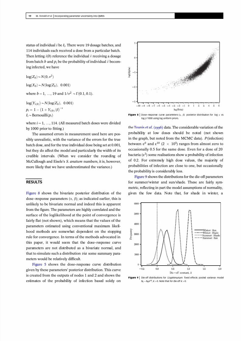
Figure 9 shows the distributions for the die-off parameters

for summer/winter and sun/shade. These are fairly sym-

metric, reflecting in part the model assumptions of normality,

given the few data. Note that, for shade in winter, a

Figure 8 9999 Dose–response curve parameters (a, b): posterior distribution for log a vs

log b/1000 using log uniform priors.

Figure 9 9999 Die-off distributions for S.typhimurium: fixed effects pooled variance mode

Nt ¼ N0e-kt , k 40. Note that for die-off k 40.




substantial proportion (14%) of the posterior die-off values

are negative, which could lead to the inference of no die-off

under these conditions.

Figure 4 shows the daily sunlight data for winter or

summer, and for both periods it can be seen that the majority

of days were neither cloudy, overcast or rainy, but attained

the maximum possible number of sunlight hours.

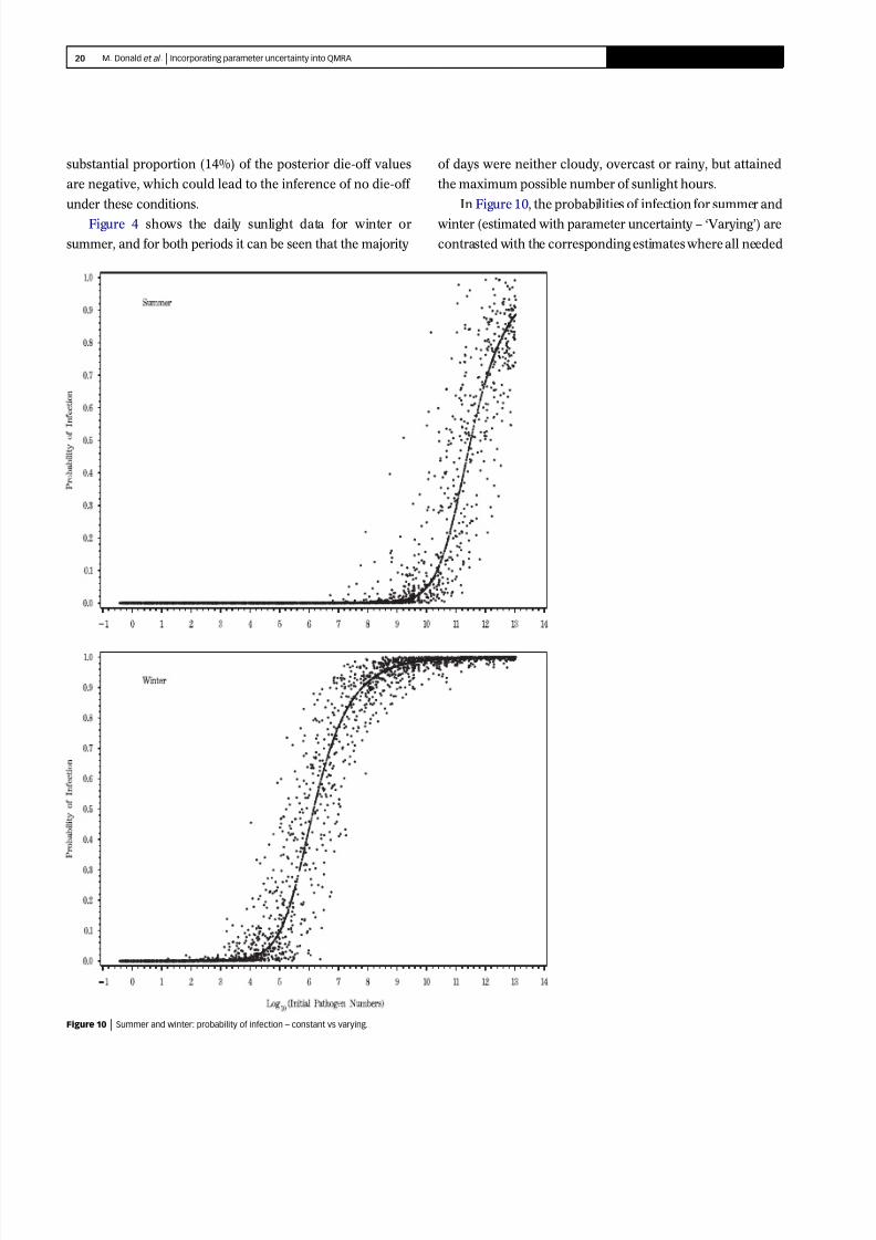
In Figure 10, the probabilities of infection for summer and

winter (estimated with parameter uncertainty – ‘Varying’) are

contrasted with the corresponding estimates where all needed

Figure 10 9999 Summer and winter: probability of infection – constant vs varying.




values have been plugged in as constants (‘Constant’). This

figure shows the addition of considerable variation when the

underlying data and their model are incorporated in the risk

assessment model. When most of the probabilities lie below

0.5, the additional uncertainty increases the range of prob-

abilities, thereby giving an increased likelihood of infection.

When most of the probabilities lie above 0.5, the added

uncertainty again gives a wider range and therefore includes

lower probabilities of infection in comparison with the model

using a constant.

Box plots for the probability of infection for 15 initial dose

groups (Figure 11) indicate that, if the infection probabilities

are not close to zero or one, the uncertainty is very greatly

increased. Thus, including parameter uncertainty could make

a very great difference to conclusions about risk. Table 3 gives

summary statistics for the initial doses by grouping. Table 2

gives summary statistics for the probability of infection for

each of these groupings shown in the graphs (Figure 11).

Thus, in Table 2, in dose grouping 8, the mean probability of

infection for winter when the constants are used is 0.82 with a

90% CI (0.73, 0.89), compared with 0.78 (0.43, 0.96) for

the varying parameters, again more than double the spread.

Table 3 shows that the initial dose range for dose grouping 8

is 6.4 106 to 5.52 107 with a median dose of 1.89 107

cells. Looking at the summer scenarios for dose grouping 12

(Table 2), the mean probability of infection is 0.25 with 90%

CI (0.12, 0.40) using constants, compared with a mean

probability of infection of 0.30 (0.04, 0.72), when parameters

are drawn with uncertainty from their distributions. This

equates to a difference in interval width of 0.68 versus 0.28.

That is, using varying parameters the credible interval covers

two-thirds of the probability scale, whereas using constants

the interval is one-third of the scale, constituting a very

substantial difference.

The effect of the uncertainty induced by the uncertainty of

the die-off parameters was so great that it seemed useful to

estimate the probability of infection for the initial dose

(divided by 1000) allowing no die-off, to show the effect of

the uncertainty induced by the dose–response parameters

alone. Figure 12 shows the effect of including the uncertainty

of the parameter estimates for dose–response when no die-off

is considered. The results for each grouping are shown in

Tables 2 and 3. Thus, for dose grouping 8, using constants

only, the 90% interval is (0.16, 0.48), but (0.12, 0.56) with

varying parameters, a difference in width of 0.32 to 0.44. This

is a considerable difference when the response lies between 0

and 1. From Table 3, this group is seen to encompass doses

from 6.4 103 to 5.5 104 cells.

Figure 13 shows the additional uncertainty in the prob-

abilities of infection from the dose–response model which

results from the errors-in-variables model. The 95% credible

intervals for the probability of infection when error is

assumed in the dose are considerably wider, but also the

mean probability of infection has moved to the left, indicating

a higher probability of infection for a dose than when the

probability is estimated without recognising that the dose is

measured with error. The additional uncertainty operates to

make the probability of infection markedly higher at lower

doses. (Note that none of the results discussed in the ‘riskFigure 11 9999 Summer and winter: probability of infection – constant vs varying by ranked

initial pathogen number groups.




Table 2 9999 Summary statistics for P(infected) over groupings

Group Period Type Mean Std. Median q5 q95

7 No die-off Constant 0.07 0.001 0.06 0.03 0.14

Varying 0.10 0.003 0.07 0.02 0.27

Summer Constant 0.00 0.000 0.00 0.00 0.00

Varying 0.00 0.000 0.00 0.00 0.00

Winter Constant 0.57 0.004 0.58 0.41 0.71

Varying 0.54 0.009 0.56 0.11 0.85


Varying 0.34 0.005 0.33 0.12 0.56

Summer Constant 0.00 0.000 0.00 0.00 0.00

Varying 0.00 0.000 0.00 0.00 0.00

Winter Constant 0.82 0.002 0.83 0.73 0.89

Varying 0.78 0.006 0.82 0.43 0.96


Varying 0.67 0.004 0.68 0.49 0.81

Summer Constant 0.00 0.000 0.00 0.00 0.00

Varying 0.01 0.001 0.00 0.00 0.04

Winter Constant 0.93 0.001 0.93 0.90 0.95

Varying 0.91 0.003 0.93 0.76 0.99


Varying 0.85 0.002 0.86 0.76 0.94

Summer Constant 0.01 0.000 0.01 0.00 0.01

Varying 0.04 0.004 0.01 0.00 0.20

Winter Constant 0.97 0.000 0.97 0.96 0.98

Varying 0.95 0.002 0.97 0.87 1.00


Varying 0.94 0.001 0.95 0.87 0.99

Summer Constant 0.05 0.001 0.04 0.02 0.10

Varying 0.12 0.006 0.05 0.01 0.48

Winter Constant 0.99 0.000 0.99 0.98 0.99

Varying 0.98 0.001 0.99 0.93 1.00


Varying 0.97 0.001 0.98 0.93 1.00

Summer Constant 0.25 0.003 0.24 0.12 0.40

Varying 0.30 0.008 0.26 0.04 0.72

Winter Constant 1.00 0.000 1.00 0.99 1.00

Varying 0.99 0.001 1.00 0.96 1.00

q5: 5th percentile of posterior distribution.

q95: 95th percentile of posterior distribution.




assessment’ include this modification to nodes 6 and 7 of

Figure 3.)

DISCUSSION

The extended QMRA model was expressed as a Bayesian

model and analysed using a simulation-based approach,

namely Markov chain Monte Carlo (MCMC) to estimate

distributions of the probability of infection, thereby taking

into account the uncertainty associated with parameter esti-

mates needed in the risk assessment, automatically and more

satisfactorily. In general, when parameter uncertainty is taken

into account, it is typical to assume that the parameter

estimate is normally distributed, which it may well not be.

The manner in which uncertainty is incorporated in

Table 3 9999 Summary statistics for groupings: group initial pathogen numbers/doses

Group Mean pathogens Std. Median Min. Max.

0 1.21 100 2.70 10-2 1.06 100 3.70 10-1 2.81 100

1 8.53 100 1.80 10-1 7.37 100 2.82 101 1.99 101

2 7.41 101 1.71 100 6.17 101 1.99 101 1.74 102

3 5.68 102 1.23 101 4.81 102 1.75 102 1.28 103

4 4.29 103 9.65 101 3.59 103 1.30 103 1.03 104

5 3.89 104 9.36 102 3.20 104 1.03 104 9.64 104

6 3.38 105 7.61 103 2.87 105 9.70 104 7.97 105

7 2.75 106 6.19 104 2.31 106 8.00 105 6.40 106

8 2.29 107 5.32 105 1.89 107 6.40 106 5.52 107

9 1.83 108 3.96 106 1.59 108 5.53 107 4.14 108

10 1.52 109 3.63 107 1.27 109 4.14 108 3.67 109

11 1.16 1010 2.50 108 9.88 109 3.68 109 2.69 1010

12 8.35 1010 1.72 109 7.28 1010 2.70 1010 1.89 1011

13 6.09 1011 1.35 1010 5.01 1011 1.90 1011 1.38 1012

14 4.57 1012 1.0 1011 3.93 1012 1.38 1012 1.07 1013

For the no die-off results, the doses are 1/1000th of these.

Figure 12 9999 Probability of infection (no die-off): using constant vs varying parameters for

beta-binomial distribution.

Figure 13 9999 Comparison of the dose–response curves for S. anatum with 95% credible

intervals, estimated with and without ‘errors-in-variables’.




the extended model allows the experimental data to dictate the

distribution of the parameter uncertainty and allows the

possibility of asymmetry and long tails. The Bayesian frame-

work permits embedding of several unrelated models in a

single risk assessment, via directed acyclic graphs (DAGs),

and may be compared with more conventional risk assess-

ments, where parameter estimates and their associated dis-

tributional assumptions are used. As examples of such risk

assessments, see, for example, Whiting & Buchanan (1997),

Tanaka et al. (1998), Pouillot et al. (2004) and Gerba et al.

(2008).

This approach may be compared with that proposed by

other researchers (Teunis et al. 1997; Haas et al. 1999) who

prepare a bootstrap sample of parameter estimates for the

dose–response curve, thereby allowing for non-normality,

prior to running the risk assessment. However, despite this

being the method recommended in Haas et al. (1999), most

risk assessments take their dose–response parameters as

constants. It would seem that bootstrapping, choosing a size

for the bootstrap sample and incorporating the resultant

bootstrap sample into the simulation framework is generally

discouraging for most practitioners. When the interest in a

risk assessment involves tails of distributions or upper per-

centiles, it is critical not to ignore the tail behaviours of the

fitted distributions. The method we propose permits all such

asymmetries and uncertainties to be easily incorporated. In

this particular case, where the dose–response parameters are

correlated, the problem of simulation is particularly difficult,

since the two parameters are not bivariate normal. Hence,

when the dose–response curve is a beta-Poisson, some

appropriate method must be used to capture the bivariate

behaviour. Haas (1999) proposes a further method based on

rank coefficients. This method is again complex to imple-

ment, whereas here we argue that using MCMC via Win-

BUGS is not.

There are so little data used in the estimation of the die-

off coefficients that there is little evidence of asymmetry.

Nonetheless, using data rather than previously estimated

constants ensures that uncertainty is propagated properly

throughout the simulation. Had the ‘shoulder’ equation of

Sinton et al. (2007) been considered appropriate, the same

problem of correlated parameter estimates for the curve fit

would again be as strongly evident as they are for the dose–

response equation.

MCMC simulation and estimation has been available for

some time, but is rarely used in the context of risk assessment

as described here. Kelly & Smith (2009) present a simple

primer of MCMC methods for this purpose and, in particular,

discuss its use in fitting hierarchical models and in dealing

appropriately with missing and uncertain data. Messner et al.

(2001) use an MCMC approach to perform a meta-analysis

using hierarchical MCMC modelling to develop a dose–

response curve for C. parvum. The same approach is taken

by Qian et al. (2004) who use MCMC to fit a hierarchical

model to perform a meta-analysis for various studies of

protozoan inactivation by UV light. Delignette-Muller et al.

(2006) used a complex hierarchical model to describe the

growth of Listeria in cold-smoked salmon and then used this

to develop a further model for the time necessary to reach

particular pathogen numbers, with the second model import-

ing the uncertainty implicit in the original data.

Paulo et al. (2005) undertook a risk assessment, which

closely parallels our approach: the parameter estimation for

various submodels and the assessment of dietary exposure to

pesticides (as a final node) was accomplished in the one

MCMC model. Like the models of Paulo et al. (2005), the

model presented in this paper differs substantially from the

majority of risk assessments in two main ways. Firstly, it

embeds the primary data (for dose–response, Salmonella die-

off and doses) within the simulation itself, thus incorporating

directly the uncertainties of the data, together with the

(unknown) correlation structures. That is, no summary data

are used and no process is represented by a constant. Sec-

ondly, by putting these together in a directed acyclic graph

(DAG) and using MCMC, the model allows us to simulta-

neously estimate all the parameters currently used in a

QMRA, together with the risks in which we are interested.

Here, every parameter, however disparate, is estimated

simultaneously with the risk simulation. This permits all

parameter uncertainty to be propagated throughout the risk

assessment by incorporating all relevant data seamlessly into

the one directed acyclic graph. Thus, ideally, the data nodes

might consist of microbial cell numbers post-treatment, dose–

response data and microbial numbers prior to treatment

(thereby allowing estimation of the log-reduction constants

and a potential comparison of the two methods of estima-

tion), die-off data and users’ consumption behaviour data.

This method means that there is no necessity for prior boot-




strap simulations, as in Cullen & Frey (1999)’s ‘two-dimen-

sional’ approach to fitting ‘uncertainty’ and ‘variability’: the

models and the methods are explicit and transparent.

In summary, we have demonstrated a method for incor-

porating parameter uncertainty, which does not require com-

plex simulation methods. Where a risk assessor is trying to do

more than arrive at a point estimate, and is running Monte

Carlo simulations such as offered by @Risk (Palisade 2008),

this method allows risk uncertainty to be satisfactorily

described without resorting to two-step estimation proce-

dures. It is also far more transparent than a spreadsheet

approach where operations and their sequencing can be

difficult to discern. This method incorporates all the original

data used to derive the required parameters for a QMRA into

the QMRA, whereas in the more traditional approach these

parameters are derived prior to undertaking the risk assess-

ment and are ‘plugged’ into the assessment. We would

recommend it as a simple, transparent method which should

be incorporated into a risk assessor’s armoury.

CONCLUSIONS

The aim of the study was twofold: (i) to indicate the potential

problems arising from failure to include the uncertainty of

parameter estimates in risk assessments and (ii) to illustrate

the superiority of estimating the parameters to be used in the

risk assessment simultaneously with the risk assessment.

When one considers the ‘banana-shaped’ bivariate graph for

the dose–response parameters (a, b) and its long left tail

presented in Figure 8, there is little doubt that the simulta-

neous estimate of all parameters of interest is a better meth-

odology to use. The techniques and programs used to derive

such estimates are now readily available.

Our analysis indicated that, where dose ranges are either

extremely large or small, estimating risk by including the

uncertainty in the underlying parameters makes little differ-

ence in the possible ranges for the probability of infection.

However, when the dose is within the range where the risk is

neither very close to one nor zero, the inclusion of uncer-

tainty in the parameters may make a marked difference in the

possible ranges for the probability of infection.

However, the results of this study highlight the superiority

of models developed directly from data for finding more

realistic estimates of uncertainty. In practical terms, we

would advocate that workers in this field report comprehen-

sive data. Commonly, reported results only include a range

and a mean, occasionally a standard deviation, and often not

even the number of observations used. These are generally

insufficient to permit adequate estimation of risk. In addition,

there is a failure to acknowledge, let alone include, the

uncertainty which results from small experiments. For the

methodology advanced in this paper, we would recommend,

firstly, that all data from experiments leading to parameters

needed in a risk assessment be in the public domain, parti-

cularly when their interpretation may have important impli-

cations for public health. A major limitation imposed on this

study was the inability to access data collected by, or on

behalf of, any Australian water utility, much of which is

mandated by law or regulation. Thus, our final recommenda-

tion is that such data be made publicly available. Journals

may make a difference in the short term by insisting on this

for data forming the basis of a published paper.

REFERENCES

Brandl, M. T. & Amundson, R. 2008 Leaf age as a risk factor

in contamination of lettuce with Escherichia coli o157: H7

and Salmonella enterica. Appl. Environ. Microbiol. 74(8),

2298–2306.

Bureau of Meteorology 2010 (e-mail) 2010jr12235*** student/request

for data, forecasts or other services/wa/climate and past

weather*** (jr- [sec¼ unclassified]. e-mail: climate.wa@bom.

gov.au. http://www.bom.gov.au.

Cullen, A. C. & Frey, H. C. 1999 Probabilistic Techniques in Exposure

Assessment: A Handbook for Dealing with Variability and Uncer-

tainty in Models and Inputs. Plenum Press, New York.

Delignette-Muller, M. L., Cornu, M., Pouillot, R. & Denis, J. B. 2006 Use

of Bayesian modelling in risk assessment: application to growth of

listeria monocytogenes and food flora in cold-smoked salmon. Int.

J. Food Microbiol. 106(2), 195–208.

Fuller, W. A. 1987 Measurement Error Models. Wiley, New York.Gerba, C. P., Campo, N. C.-d., Brooks, J. P. & Pepper, I. L. 2008 Expo-

sure and risk assessment of salmonella in recycled residuals. Wat.

Sci. Technol. 57(7), 1061–1065.

Gibbs, R. A. 1995 Die-off of Human Pathogens in Stored Wastewater

Sludge and Sludge Applied to Land. Technical report, Urban

Water Research Association of Australia, Water Services Associa-

tion of Australia, Melbourne.

Gibbs, R. A. & Ho, G. E. 1993 Health risks from pathogens in untreated

wastewater sludge: implications for australian sludge management

guidelines. Water 20(1), 17–22.


http://dx.doi.org/10.1128/AEM.02459-07





http://www.bom.gov.au/

http://dx.doi.org/10.1016/j.ijfoodmicro.2005.06.021



http://dx.doi.org/10.2166/wst.2008.235


http://dx.doi.org/10.1016/0273-1223(95)00247-K

http://dx.doi.org/10.1016/0273-1223(95)00247-K

http://dx.doi.org/10.1016/0273-1223(95)00247-K

http://dx.doi.org/10.1016/0273-1223(95)00247-K

http://dx.doi.org/10.1016/0273-1223(95)00247-K

http://dx.doi.org/10.1016/0273-1223(95)00247-K






http://www.bom.gov.au/






Gibbs, R. A., Hu, C. J., Ho, G. E., Phillips, P. A. & Unkovich, I. 1995

Pathogen die-off in stored wastewater sludge. Wat. Sci. Technol.

31(5–6), 91–95.

Haas, C. N. 1999 On modeling correlated random variables in risk

assessment . Risk Anal. 6, 1205–1214.

Haas, C. N., Rose, J. B. & Gerba, C. P. 1999 Quantitative Microbial Risk

Assessment . Wiley, New York.

Hijnen, W. A., Beerendonk, E., Smeets, P. & Medema, G. 2004

Elimination of Micro-organisms by Water Treatment Processes.

Technical report. Kiwa NV, Nieuwegein.

Hijnen, W. A., Dullemont, Y. J., Schijven, J. F., Hanzens-Brouwer, A. J.,

Rosielle, M. & Medema, G. 2007 Removal and fate of cryptospor-

idium parvum, clostridium perfringens and small-sized centric

diatoms (stephanodiscus hantzschii) in slow sand filters. Wat.

Res. 41, 2151–2162.

Kelly, D. L. & Smith, C. L. 2009 Bayesian inference in probabilistic risk

assessment–the current state of the art . Reliab. Engng. Syst. Safety.

94(2), 628–643.

Lunn, D. J., Thomas, A., Best, N. & Spiegelhalter, D. J. 2000 A Bayesian

modelling framework: concepts, structure and extensibility.

Statist. Comput. 10(4), 325–337.

Marks, H. M., Coleman, M. E., Lin, C. T. J. & Roberts, T. 1998 Topics in

microbial risk assessment: dynamic flow tree process. Risk Anal.

18(3), 309–328.

McCullough, N. B. & Eisele, C. W. 1951 Experimental human Salmo-

nellosis: I. Pathogenicity of strains of Salmonella meleagridis and

Salmonella anatum obtained from spray-dried whole egg. J. Infect.

Dis. 88(3), 278–289.

Messner, M. J., Chappell, C. L. & Okhuysen, P. C. 2001 Risk assessment

for cryptosporidium: a hierarchical Bayesian analysis of human

dose response data. Wat. Res. 35(16), 3934–3940.

National Resource Management Ministerial Council and Environment

Protection and Heritage Council (NRMMC) 2006 Australian

Guidelines for Water Recycling: Managing Health and Environ-

mental Risks (Phase1) 2006. Australian Government. Available

online: http://www.ephc.gov.au/taxonomy/term/39

Oscar, T. 2004 Dose-response model for 13 strains of Salmonella. Risk

Anal. 24(1), 41–49.

Palisade Corporation 2008 @Risk5.0. Available at: http://www.palisa

de.com/risk/.

Paulo, M. J., Voet, H. v. d., Jansen, M. J.W., Braak, C. J. F. t. & Klaveren,

J. D. v. 2005 Risk assessment of dietary exposure to pesticides using

a Bayesian method. Pest Mngmnt. Sci. 61(8), 759–766.

Pouillot, R., Beaudeau, P., Denis, J.-B. & Derouin, F. 2004 A quantita-

tive risk assessment of waterborne cryptosporidiosis in France

using second-order Monte Carlo simulation. Risk Anal. 24(1),

1–17.

Qian, S. S., Donnelly, M., Schmelling, D. C., Messner, M., Linden, K. G.

& Cotton, C. 2004 Ultraviolet light inactivation of protozoa

in drinking water: a Bayesian meta-analysis. Wat. Res. 38(2),

317–326.

Sidhu, J. P. S., Hanna, J. & Toze, S. G. 2008 Survival of enteric

microorganisms on grass surfaces irrigated with treated effluent .

J. Wat. Health. 6(2), 255–262.

Sinton, L., Hall, C. & Braithwaite, R. 2007 Sunlight inactivation of

campylobacter jejuni and salmonella enterica, compared with

escherichia coli, in seawater and river water. J. Wat. Health

5(3), 357–365.

Tanaka, H., Asano, T., Schroeder, E. D. & Tchobanoglous, G. 1998

Estimating the safety of wastewater reclamation and reuse

using enteric virus monitoring data. Wat . Environ. Res. 70(1),

39–51.

Teunis, P. F. M., Medema, G. J., Kruidenier, L. & Havelaar, A. H. 1997

Assessment of the risk of infection by cryptosporidium or gia-

rdia in drinking water from a surface water source. Wat. Res. 31,

1333–1346.

Teunis, P. F. M., van der Heijden, O., van der Giessen, J. W. B. &

Havelaar, A. H. 1996 The Dose–Response Relation in Human

Volunteers for Gastro-intestinal Pathogens. Report no.

2845500002. National Institute of Public Health and the Environ-

ment (RIVM), Bilthoven, The Netherlands.

Wand, M. P. 2009 Semiparametric regression and graphical models.

Austral. NZ J. Statist. 51(1), 9–41.

Whiting, R. C. & Buchanan, R. L. 1997 Development of a quantitative

risk assessment model for salmonella enteritidis in pasteurized

liquid eggs. Int. J. Food Microbiol. 36, 111–125.

First received 20 July 2009; accepted in revised form 18 May 2010. Available online 20 October 2010


http://dx.doi.org/10.1023/A:1007047014741

http://dx.doi.org/10.1023/A:1007047014741

http://dx.doi.org/10.1016/j.watres.2007.01.056



http://dx.doi.org/10.1016/j.ress.2008.07.002


http://dx.doi.org/10.1023/A:1008929526011

http://dx.doi.org/10.1023/A:1008929526011

http://dx.doi.org/10.1111/j.1539-6924.1998.tb01298.x


http://dx.doi.org/10.1016/S0043-1354(01)00119-1

http://dx.doi.org/10.1016/S0043-1354(01)00119-1

http://dx.doi.org/10.1016/S0043-1354(01)00119-1

http://www.ephc.gov.au/taxonomy/term/39

http://dx.doi.org/10.1111/j.0272-4332.2004.00410.x

http://dx.doi.org/10.1111/j.0272-4332.2004.00410.x

http://www.palisade.com/risk/


http://dx.doi.org/10.1002/ps.1060


http://dx.doi.org/10.1111/j.0272-4332.2004.00407.x

http://dx.doi.org/10.1111/j.0272-4332.2004.00407.x

http://dx.doi.org/10.1111/j.0272-4332.2004.00407.x



http://dx.doi.org/10.2166/wh.2008.029

http://dx.doi.org/10.2166/wh.2008.029

http://dx.doi.org/10.2166/wh.2008.029

http://dx.doi.org/10.2166/wh.2007.031

http://dx.doi.org/10.2166/wh.2007.031

http://dx.doi.org/10.2166/wh.2007.031

http://dx.doi.org/10.2175/106143098X126874

http://dx.doi.org/10.2175/106143098X126874

http://dx.doi.org/10.2175/106143098X126874

http://dx.doi.org/10.1016/S0043-1354(96)00387-9

http://dx.doi.org/10.1016/S0043-1354(96)00387-9

http://dx.doi.org/10.1111/j.1467-842X.2009.00538.x


http://dx.doi.org/10.1016/S0168-1605(97)01262-2

http://dx.doi.org/10.1016/S0168-1605(97)01262-2

http://dx.doi.org/10.1016/S0168-1605(97)01262-2

http://dx.doi.org/10.1016/S0168-1605(97)01262-2

http://dx.doi.org/10.1016/S0168-1605(97)01262-2

http://dx.doi.org/10.1016/S0168-1605(97)01262-2


http://dx.doi.org/10.1016/S0043-1354(96)00387-9

http://dx.doi.org/10.1016/S0043-1354(96)00387-9

http://dx.doi.org/10.2175/106143098X126874

http://dx.doi.org/10.2175/106143098X126874

http://dx.doi.org/10.2166/wh.2007.031

http://dx.doi.org/10.2166/wh.2007.031

http://dx.doi.org/10.2166/wh.2007.031

http://dx.doi.org/10.2166/wh.2008.029

http://dx.doi.org/10.2166/wh.2008.029



http://dx.doi.org/10.1111/j.0272-4332.2004.00407.x

http://dx.doi.org/10.1111/j.0272-4332.2004.00407.x

http://dx.doi.org/10.1111/j.0272-4332.2004.00407.x





http://dx.doi.org/10.1111/j.0272-4332.2004.00410.x

http://www.ephc.gov.au/taxonomy/term/39

http://dx.doi.org/10.1016/S0043-1354(01)00119-1

http://dx.doi.org/10.1016/S0043-1354(01)00119-1

http://dx.doi.org/10.1016/S0043-1354(01)00119-1



http://dx.doi.org/10.1023/A:1008929526011

http://dx.doi.org/10.1023/A:1008929526011






http://dx.doi.org/10.1023/A:1007047014741

http://dx.doi.org/10.1023/A:1007047014741

donald uncertainty qmra

Documents