does school quality matter? returns to education and...

Does School Quality Matter? Returns to Education and the Characteristics ofPublic Schools in the United States

David Card; Alan B. Krueger

The Journal of Political Economy, Vol. 100, No. 1. (Feb., 1992), pp. 1-40.

Stable URL:

http://links.jstor.org/sici?sici=0022-3808%28199202%29100%3A1%3C1%3ADSQMRT%3E2.0.CO%3B2-U

The Journal of Political Economy is currently published by The University of Chicago Press.

Your use of the JSTOR archive indicates your acceptance of JSTOR's Terms and Conditions of Use, available athttp://www.jstor.org/about/terms.html. JSTOR's Terms and Conditions of Use provides, in part, that unless you have obtainedprior permission, you may not download an entire issue of a journal or multiple copies of articles, and you may use content inthe JSTOR archive only for your personal, non-commercial use.

Please contact the publisher regarding any further use of this work. Publisher contact information may be obtained athttp://www.jstor.org/journals/ucpress.html.

Each copy of any part of a JSTOR transmission must contain the same copyright notice that appears on the screen or printedpage of such transmission.

The JSTOR Archive is a trusted digital repository providing for long-term preservation and access to leading academicjournals and scholarly literature from around the world. The Archive is supported by libraries, scholarly societies, publishers,and foundations. It is an initiative of JSTOR, a not-for-profit organization with a mission to help the scholarly community takeadvantage of advances in technology. For more information regarding JSTOR, please contact [email protected].

http://www.jstor.orgTue Jul 3 19:14:12 2007

http://links.jstor.org/sici?sici=0022-3808%28199202%29100%3A1%3C1%3ADSQMRT%3E2.0.CO%3B2-U

http://www.jstor.org/about/terms.html

http://www.jstor.org/journals/ucpress.html

Does School Quality Matter? Returns to Education and the Characteristics of Public Schools in the United States

David Card and Alan B. Krueger Princetor1 Ur~iversity

This paper estimates the effects of school quality-measured by the pupillteacher ratio, average term length, and relative teacher pay- on the rate of return to education for men born between 1920 and 1949. Using earnings data from the 1980 census, we find that men who were educated in states with higher-quality schools have a higher return to additional years of schooling. Rates of return are also higher for individuals from states with better-educated teachers and with a higher fraction of female teachers. Holding constant school quality measures, however, we find no evidence that parental income or education affects average state-level rates of return.

Beginning with the highly influential Coleman report (Coleman et al. 1966), researchers have found little, if any, association between the quality of schools and student achievement on standardized tests (see Hanushek [I9861 for a recent survey). On the basis of these findings, it is now widely argued that increases in public school funding have few important benefits for students. This conclusion, although politi- cally popular, contradicts two other strands of evidence on the quality of schooling. On one hand, the small number of studies that have directly correlated school quality and earnings have found a significantly positive relationship between them (Welch 1966; Morgan and

We are grateful to Michael Boozer and Dean Hyslop for outstanding research assis- tance. We have also benefited from the comments of Richard Freeman, Claudia Goldin, Jean Grossman, James Heckman, Lawrence Katz, Robert Margo, Sherwin Rosen, an anonymous referee, and seminar participants at several institutions. Financial support from the Princeton Industrial Relations Section is gratefully acknowledged.

[Journal of Pohtccal Economy, 1992, vol. 100, no. I] O 1992 by The University of Chicago. All rights reserved. 0022-3808/92/0001-0003$01.50

2 JOURNAL OF POLITICAL ECONOMY

Sirageldin 1968;Johnson and Stafford 1973; Wachtel 1976; Rizzuto and Wachtel 1980). On the other hand, much of the gain in black- white relative earnings over the past century has been attributed to growth in the relative quality of black schooling (Welch 1967, 1973a, 19736; Freeman 1976; Smith and Welch 1989).

There are several possible explanations for the conflicting evidence. Studies of earnings and school quality typically focus on the correlation between school characteristics (such as per capita expenditure) and the average earnings of students educated in a school district. One can easily argue that family background variables affect both education expenditures and labor market earnings. In this case, the correlation of school quality and earnings is potentially spurious. From the opposite perspective, one can argue that test scores are an imperfect measure of school performance. Indeed, although earnings and test scores are correlated, they are by no means identical.' Factors that affect subsequent labor market achievement may have a much smaller impact on test scores. Furthermore, the relation between school quality and test scores at the eighth or twelfth grade fails to capture any effects of school quality on subsequent learning.

This paper presents an extensive analysis of the relation between earnings and school quality for cohorts of men born between 1920 and 1949. We use the relatively large samples available from the 1980 census to estimate rates of return to education by state of birth and cohort. We then relate rates of return to schooling to objective measures of school quality, including pupillteacher ratios, relative wages of teachers, and the length of the school term.2

Our procedures overcome at least some of the objections to earlier studies of earnings and school quality. First, our statistical models include unrestricted state of birth effects and therefore control for any differences in the mean earnings of men born in different states. T o the extent that differences in family characteristics raise or lower earnings for all levels of schooling attainment, our estimated rates of return are purged of any effects of differential family background. Second, we control for systematic differences in the returns to education associated with an individual's current region of residence. We thereby eliminate relative supply or demand effects that raise or lower the returns to education in different parts of the country. Fi- nally, in much of our analysis we incorporate permanent state-specific

For example, the addition of test score information to the earnings models reported by Griliches and Mason (1972, table 3) improves the explanatory power of their models by less than one-half of a percentage point.

Our approach is conceptually similar to that of Behrman and Birdsall (1983), who relate the returns to schooling among young Brazilian men to the average years of education of teachers in each individual's region of residence.

3 RETURNS TO EDUCATION

effects in the return to education and use only the within-state variation among consecutive cohorts to identify the effects of school quality on the returns to education.

Our results indicate that there is substantial variation in the rate of return to education across individuals born in different states and at different times. Much of this variation is associated with differences in the quality of schooling. We find that rates of return are higher for individuals who attended schools with lower pupillteacher ratios and higher relative teacher salaries. For example, our estimates suggest that a decrease in the pupillteacher ratio by five students is associated with a 0.4-percentage-point increase in the rate of return to schooling. Similarly, a 10 percent increase in teachers' pay is associated with a 0.1-percentage-point increase in the rate of return to schooling. We also find that returns are linked to higher education among teachers. Controlling for measures of school quality, however, we find no evidence that returns to education are related to the income or schooling levels of the parents' generation.

Our main focus is on the relation between school quality and the rate of return to education. Changes in the slope of the earnings- schooling relation, however, do not necessarily raise average earnings. For example, the earnings gains of better-educated workers may come at the expense of the less educated. On the other hand, changes in the quality of schooling may affect the average level of education as well as the marginal return to added years of schooling. T o address these issues we present some simple "reduced-form" evidence on the relationship between school quality and the mean levels of education and earnings. Controlling for any permanent differences across individuals born in different states, we find significant positive effects of school quality on both the average years of schooling and mean earnings of students. The reduced-form results suggest that increases in school quality affect subsequent earnings by increasing the number of years of completed education and by increasing the return to each year of schooling.

I. An Empirical Framework for Modeling Returns to Schooling

Our goal is to relate the returns to education earned by individuals educated in different states to the characteristics of the public school system during the time they attended school. To fix ideas it is useful to assume that individuals attend school in their state of birth and to ignore private schooling. (The effects of these simplifications are explored below.) Let yii, represent the logarithm of weekly earnings for individual i, born in state j in cohort c and currently living in state


k of region r , and let Eqk, represent the years of education completed by individual i. Suppose that earnings are determined by an equation of the form

where 9, represents a (cohort-specific) fixed effect for each state of birth, kkc represents a (cohort-specific) fixed effect for each state of residence, Xgkc represents a set of measured covariates (years of labor market experience, marital status, and an indicator for whether i lives in a standard metropolitan statistical area [SMSA]), and eijk, represents a stochastic error term. Equation (1) assumes a linear specification of the return to education, consisting of two components: a cohort and state of birth effect (y,,) and a cohort and region of residence effect (P , ) .~ These components allow observed rates of return to schooling to vary because of differences in the return to education across different regional labor markets (i.e., variation in p,,) and because of differences in the rate of return to education earned by individuals in a given state of birth and cohort group in any labor market (i.e., variation in yt).

Notice that when we include interactions between state of birth dummies and education and another set of interactions between region of residence dummies and education, the state of birth-specific contribution to the return to education is identified by individuals who are educated in one state and move to another region. I t is the shift i n the return to education attributable to schooling i n a particular state that we seek to explain by differences in school quality across states and over tzme.

Specifically, we hypothesize that the state of birth components in the return to education depend on the quality of the public schools, and possibly on a set of state-specific constants:

where Q,, is a vector of measures of the quality of the education system in state j during the time that cohort c attended school. In this specification any permanent differences in the returns to education arising, for example, from differences in the distributions of ability across states are absorbed by the state of birth effects (a,) in (2).

Under these assumptions, the effects of a particular measure of education quality can be obtained in one step by estimating a log- linear earnings function that includes state of birth effects, state of residence effects, interactions of region of residence with education,

We normalize the coefficients y,, and p,, by setting C,f,,p,, = 0, where f,, is the fraction of cohort c living in one of the nine census regions.


and interactions of education with state of birth effects and the quality measures for state j and cohort c. However, we prefer to proceed in two steps: first, estimating the average rate of return to education for individuals born in cohort c in state j , controlling for state of birth, state of residence, and any regional differences in the return to education; and then using a second-step regression to relate the estimated rates of return (by cohort and state of birth) to the quality variables.

The two-step procedure has several important advantages. In the first place, it provides a convenient reduction of the data and allows us to illustrate the diversity in the returns to education and their relation to measures of school quality. A two-step procedure also facilitates extremely general models of the earnings function (I) , including models with cohort-specific state of birth and state of residence effects, and models with permanent state of birth effects in the return to education. In addition, we can incorporate a simple correction for the interstate mobility of children. A disadvantage of the two-step procedure is that cohorts must be defined fairly broadly to obtain reliable estimates of the state- and cohort-specific returns to education. In the analysis below we use 10-year intervals of births. This aggregation eliminates any within-cohort variation in school quality or the returns to education and leads to some efficiency loss. Since individuals are assigned the mean levels of school quality for their state of birth and cohort, however, aggregation does not intro- duce classical measurement error into the quality measures (see Gril- iches 1986, p. 1478).

A. Functional Form

The assumption of a linear relation between schooling and (log) earnings is widely used in applied studies of earnings and is often found to perform as well as or better than simple alternatives (e.g., Heckman and Polachek 1974). However, most studies pool samples of individuals from different states and birth cohorts with no allowance for regional or cohort differences in returns. It is conceivable that the log earnings-schooling relation is approximately linear in pooled samples but is nonlinear for particular subsamples. It is also conceivable that changes in the quality of public schooling shift the returns to elementary or secondary education more (or less) than the returns to college. If so, then the specification of the return to education function should allow for kinks at 12 years of education.

In an effort to obtain some simple evidence on these issues, we estimated a series of unrestricted earnings-schooling models using narrowly defined subsamples of individuals in the 1980 census. These models include a complete set of dummy variables for 0-20 years of


a

0 2 4 6 8 10 12 14 16 18 Yeors of Comoleted Educotion

0 2 4 6 8 10 12 14 16 18 2o Years of Completed Education

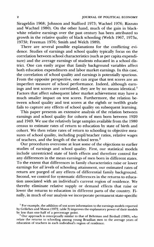
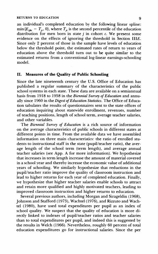
FIG. 1.-Wages vs. schooling, by cohort and state of birth: a, white men born in Alabama or Georgia; b, white men born in California.

education, as well as controls for potential labor market experience, marital status, state of residence, and residence in an SMSA.4 Figure 1 graphs the estimated return to education relationships for six of the subsamples: three cohorts of white men born in Alabama or Georgia (1920-29, 1930-39, and 1940-49) and three cohorts of white men born in California. Figure 2 graphs the estimated return to education

Specifically, the models include linear and quadratic terms in potential experience, a dummy variable for being married with spouse present, a dummy variable for residence in an SMSA, and unrestricted dummy variables for residence in each of the 50 states. Additionally, dummy variables indicating state of birth were included if the sample combined observations from more than one state. The models are estimated on subgroups of the sample described in App. B.

20

a

0 - 1 Std. Enor

A + 1 Std. Enor

0 2 1 8 10 32

r a a c0W.l.a -by

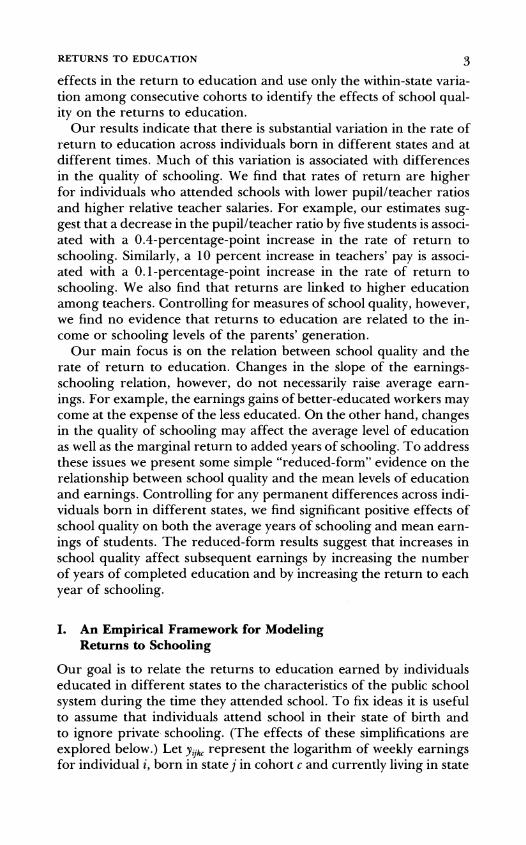
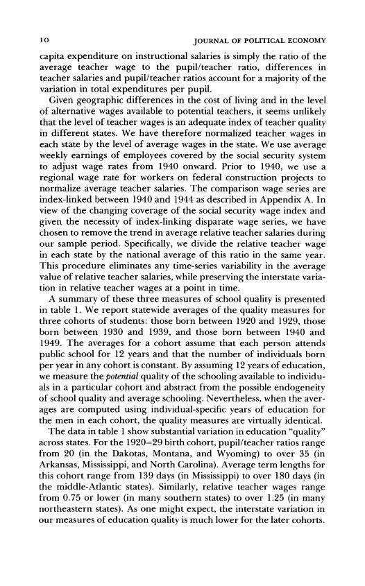
FIG. 2.-Return to single years of education: a, white men born 1920-29, nationwide; b, white men born 1930-39, nationwide; c, white men born 1940-49, nationwide.

20


relationships (together with their standard error bounds) for national samples of white men in the same three cohorts.

The figures illustrate three general findings. First, for a particular cohort and state of birth group, the earnings-education relation is approximately log-linear for levels of education above a minimum threshold. Although there is some evidence of a college graduation effect, departures from log-linearity above the threshold level are small. Second, the threshold varies widely across states and over time within states. It is relatively low for older cohorts and for individuals from states with lower average educational attainment. This phenom- enon is also evident in the national samples in figure 2: the threshold is at approximately 2 years of education for men born between 1920 and 1929, at 3 years of education for those born during 1930-39, and at 5 years for those born in 1940-49. Third, the rate of return to education (for years of education above the threshold level) is higher for later cohorts.

The positive correlation between the average educational attainment of a state of birth and cohort group and the kink or threshold point in their return to education function led us to investigate the determinants of this threshold more carefully. For each of 13 larger states (or pairs of contiguous states) and each of three 10-year birth cohorts, we first estimated a nonparametric version of the return to education function (using 20 unrestricted dummy variables) and found the approximate threshold point in the return to education relation. We then compared this point to various percentiles of the education distribution in each state-cohort group. This comparison led us to a simple empirical relation: across different cohorts and states of birth and different race groups, the threshold point corre- sponds approximately to the grade level attained by the second percentile of the education distribution of workers. For example, a simple linear regression of the estimated threshold point on the grade attained by the second percentile of the education distribution has an estimated coefficient of 0.88 with an estimated standard error of 0.13 and an R' of .57.'

Given the pattern of the nonparametric estimates of the return to education function for the larger states, in the remainder of the paper we concentrate on measuring the return to education for years of schooling above the second percentile of the education distribution of an individual's state of birth and cohort. Specifically, we replace

Further details of our investigation, including tabulations of the estimated threshold points and education percentiles, are available on request. The 13 state groups include 11 individual states (California, New York, Ohio, Texas, Pennsylvania, Illinois, Michigan, New Jersey, Massachusetts, North Carolina, and Virginia) and two pairs of states (AlabamaiGeorgia and KentuckyiTennessee).

9 RETURNS T O EDUCATION

an individual's completed education by the following linear spline: min{E+ - T,,, 0), where T,, is the second percentile of the education distribution for men born in state j in cohort c. We present some evidence on the effects of ignoring the threshold in Section I I IE. Since only 2 percent of those in the sample have levels of education below the threshold point, the estimated rates of return to years of education above the threshold turn out to be quite similar to the estimated returns from a conventional log-linear earnings-schooling model.

11. Measures of the Quality of Public Schooling

Since the late nineteenth century the U.S. Office of Education has published a regular summary of the characteristics of the public school systems in each state. These data are available on a semiannual basis from 1918 to 1958 in the Biennial Survey of Education and annu- ally since 1960 in the Digest of Education Statistics. The Office of Educa- tion tabulates the results of questionnaires sent to the state offices of education inquiring about statewide enrollment, revenues, number of teaching positions, length of school term, average teacher salaries, and other variables.

The Biennial Survey of Education is a rich source of information on the average characteristics of public schools in different states at different points in time. From the available data we have assembled information on three main characteristics: the ratio of enrolled students to instructional staff in the state (pupillteacher ratio), the average length of the school term (term length), and average annual teacher salaries (see App. A for more information). We hypothesize that increases in term length increase the amount of material covered in a school year and thereby increase the economic value of additional years of schooling. We similarly hypothesize that reductions in the pupillteacher ratio improve the quality of classroom instruction and lead to higher returns for each year of completed education. Finally, we hypothesize that higher teacher salaries enable schools to attract and retain more qualified and highly motivated teachers, leading to improved classroom instruction and higher returns to education.

Several previous authors, including Morgan and Sirageldin (1968), Johnson and Stafford (1973), Wachte1(1976), and Rizzuto and Wach- tel (1980), have used total expenditures per pupil as an index of school quality. We suspect that the quality of education is more directly linked to indexes of pupillteacher ratios and teacher salaries than to total expenditures per pupil, and indeed this is suggested by the results in Welch (1966). Nevertheless, roughly 60 percent of total education expenditures go for instructional salaries. Since the per


capita expenditure on instructional salaries is simply the ratio of the average teacher wage to the pupillteacher ratio, differences in teacher salaries and pupillteacher ratios account for a majority of the variation in total expenditures per pupil.

Given geographic differences in the cost of living and in the level of alternative wages available to potential teachers, it seems unlikely that the level of teacher wages is an adequate index of teacher quality in different states. We have therefore normalized teacher wages in each state by the level of average wages in the state. We use average weekly earnings of employees covered by the social security system to adjust wage rates from 1940 onward. Prior to 1940, we use a regional wage rate for workers on federal construction projects to normalize average teacher salaries. The comparison wage series are index-linked between 1940 and 1944 as described in Appendix A. In view of the changing coverage of the social security wage index and given the necessity of index-linking disparate wage series, we have chosen to remove the trend in average relative teacher salaries during our sample period. Specifically, we divide the relative teacher wage in each state by the national average of this ratio in the same year. This procedure eliminates any time-series variability in the average value of relative teacher salaries, while preserving the interstate variation in relative teacher wages at a point in time.

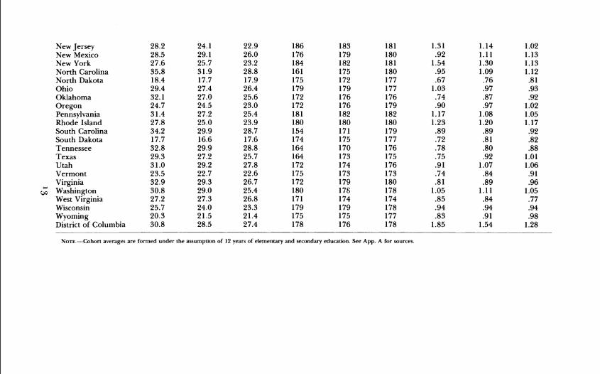
A summary of these three measures of school quality is presented in table 1. We report statewide averages of the quality measures for three cohorts of students: those born between 1920 and 1929, those born between 1930 and 1939, and those born between 1940 and 1949. The averages for a cohort assume that each person attends public school for 12 years and that the number of individuals born per year in any cohort is constant. By assuming 12 years of education, we measure the potential quality of the schooling available to individuals in a particular cohort and abstract from the possible endogeneity of school quality and average schooling. Nevertheless, when the averages are computed using individual-specific years of education for the men in each cohort, the quality measures are virtually identical.

The data in table 1 show substantial variation in education "quality" across states. For the 1920-29 birth cohort, pupillteacher ratios range from 20 (in the Dakotas, Montana, and Wyoming) to over 35 (in Arkansas, Mississippi, and North Carolina). Average term lengths for this cohort range from 139 days (in Mississippi) to over 180 days (in the middle-Atlantic states). Similarly, relative teacher wages range from 0.75 or lower (in many southern states) to over 1.25 (in many northeastern states). As one might expect, the interstate variation in our measures of education quality is much lower for the later cohorts.

1 1 RETURNS TO EDUCATION

This is particularly true of the term length variable, which falls in a narrow range for individuals born in the latest cohort.

The trends in school quality during our sample period vary widely across states. Most of the southern states show uniform improvements in quality. Other states, such as Michigan and Missouri, show almost no change in the quality variables, and some states show declines in certain dimensions of quality. The differences are most pronounced in relative teacher wages. For example, teachers in Alabama and Georgia show strong relative wage gains, and teachers in Massachu- setts, New Jersey, and New York show relative wage losses during our sample period.

111. Returns to Education by Cohort and State of Birth for White Men

In this section we present estimates of the average rates of return to education for white men born in the 48 mainland states and the District of Columbia between 1920 and 1949. We divide the samples of men born in these states into three 10-year birth cohorts and obtain estimated rates of return for 147 separate state and cohort groups. We then perform a second-step analysis of the relation between rates of return to schooling and the school quality measures in table 1. We explore the effects of some other characteristics of the school systems in each state and contrast these to the effects of some measures of family background. We also discuss the results of a simple correction for the measurement error induced by the interstate mobility of children. Finally, we present a brief analysis of the rates of return to education obtained from models that ignore the minimum thresholds highlighted in figures 1 and 2.

A. Rates of Return to Education by State and Cohort

Our estimated rates of return to education are obtained from three cohort-specific regressions fitted to individual data on log weekly earnings for 1979. The data samples are taken from the 5 percent Public-Use A Sample of the 1980 census (see App. B for details). Following the specification of equation (I) , the explanatory variables in each regression include a set of 50 indicator variables for an individual's current state of residence, a set of 48 indicator variables for an individual's state of birth, and controls for potential experience and its square, marital status, and residence within an SMSA. T o control for differences in the rate of return to education across different labor markets in the country, the models also include interactions between nine current region of residence dummies and com-

-- --

AVERAGES QUALITY FOR BORN 1920-29, 1930-39, 1940-49 (Black and White Students Combined) OF SCHOOL VARIABLES COHORTS IN AND

Alabama Arizona Arkansas California Colorado Connecticut Delaware Florida Georgia Idaho Illinois Indiana Iowa Kansas Kentucky Louisiana Maine Maryland Massachusetts Michigan Minnesota Mississippi Missouri Montana Nebraska Nevada New Hampshire

-- .- --- .-

PUPILITEACHERRATIO TERM LENGTH (Days) RELATIVETEACHERWAGE

1920-29 1930-39 1940-49 1920-29 1930-39 1940-49 1920-29 1930-39 1940-49

New Jersey New Mexico New York North Carolina North Dakota Ohio Oklahoma Oregon Pennsylvania Rhode Island South Carolina South Dakota Tennessee Texas Utah Vermont Virginia,- Washington West Virginia Wisconsin Wyoming District of Columbia

NOTE.-Cohort averages are formed under the assumption of 12 years of elementary and secondary education. See App. A for sources

'4 JOURNAL OF POLITICAL ECONOMY

pleted e d ~ c a t i o n . ~ Finally, the models include state of birth-specific interactions with individual education, where, as described in Section I, individual education is modeled as the maximum of zero and years of education over and above the second percentile of the education distribution in an individual's state of birth and cohort. These interactions are interpreted as estimates of the rate of return to education for individuals from a particular cohort and state.

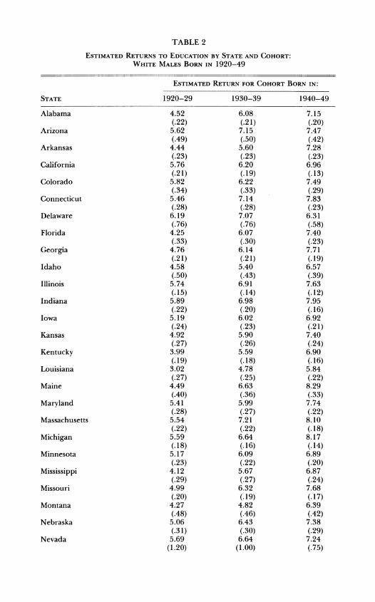
The estimated rates of return, together with their estimated sampling errors, are presented in table 2. The lower panel of the table reports the weighted means and standard deviations of the estimated returns across the 49 states, together with their correlations with the three cohort-specific quality measures. Despite the fact that the estimates are obtained from highly parameterized models (there are 158 explanatory variables in the regression equation for each cohort), the estimates are relatively precise, with standard errors in the range of 0.1-0.3 percent for most states. As the patterns in figures 1 and 2 suggest, average rates of return to education are much lower for older workers: 5.1 percent per year for the oldest cohort (age 50-59 in 1979) versus 7.4 percent for the youngest cohort (age 30-39 in 1979). The interstate dispersion in returns (corrected for sampling error) shows the opposite trend, being largest for the oldest cohort and smallest for the youngest.

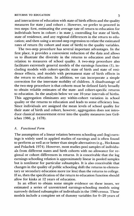
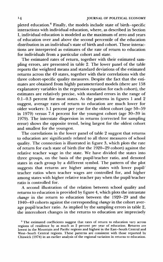
The correlations in the lower panel of table 2 suggest that returns to education are significantly related to all three measures of school quality. The connection is illustrated in figure 3, which plots the rate of return for each state of birth (for the 1920-29 cohort) against the relative teacher wage in the state. We have divided the states into three groups, on the basis of the pupillteacher ratio, and denoted states in each group by a different symbol. The pattern of the plot suggests that returns are higher among states with lower pupil1 teacher ratios when teacher wages are controlled for, and higher among states with higher relative teacher pay when the pupillteacher ratio is controlled for.

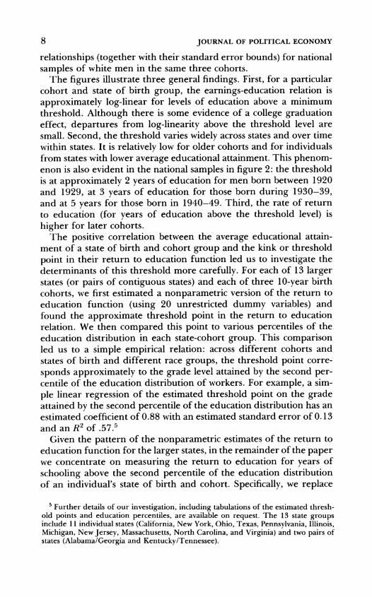
A second illustration of the relation between school quality and returns to education is provided by figure 4, which plots the intrastate change in the return to education between the 1920-29 and the 1940-49 cohorts against the corresponding change in the cohort average pupillteacher ratio. As implied by the sampling errors in table 2, the intercohort changes in the returns to education are imprecisely

The estimated coefficients suggest that rates of return to education vary across regions of residence by as much as 2 percent per year of education. Returns are lowest in the Mountain and Pacific regions and highest in the East-South Central and West-South Central regions. These patterns are consistent with those reported by Chiswick (1974) in an earlier analysis of the regional variation in returns to education.

Alabama

Arizona

Arkansas

California

Colorado

Connecticut

Delaware

Florida

Georgia

Idaho

Illinois

Indiana

Iowa

Kansas

Kentucky

Louisiana

Maine

Maryland

Massachusetts

Michigan

Minnesota

Mississippi

Missouri

Montana

Nebraska

Nevada

TABLE 2 (Continued)

New Hampshire

New Jersey

New Mexico

New York

North Carolina

North Dakota

Ohio

Oklahoma

Oregon

Pennsylvania

Rhode Island

South Carolina

South Dakota

Tennessee

Texas

Utah

Vermont

Virginia

Washington

West Virginia

Wisconsin

Wyoming

District of Columbia

Mean over all states Standard deviation Correlation with:

Pupillteacher ratio Term length Relative teacher wage

NOTE.--Column entries are estimated rates of return to education, based on samples in the 1980 census. The estimated standard deviation of returns is adjusted for the expected contribution of sampling variability. Standard errors are in parentheses.

16

0.02 1 I I I I I I I I I I I I

0.6 0.8 1 1.2 1.4 1.6 1.8

Relative Teacher Wage

FIG. 3.-Relative teacher wage vs. return to school, with high, low, and medium pupillteacher ratio indicated.

I I I I I I

Change I n Pupl l /Teacher Ra t lo -8 -6 -4 -2 0 2

FIG. 4.-Change in returns vs. change in pupillteacher ratio, 1940s cohort minus 1920s cohort.


estimated for some of the smaller states. We have therefore plotted each state observation with a circle that is proportional to the inverse sampling variance of the estimated change in returns. We have also plotted the weighted-least-squares regression line (weighted by the inverse sampling variance of the change in the estimated return) re- lating the intrastate changes in returns to the corresponding changes in the pupillteacher ratio. The figure indicates that rates of return to education rose more quickly between the 1920-29 cohort and the 1940-49 cohort in states that experienced a larger reduction in pupil1 teacher ratios.

B . Rates of Return and the Quality of Schools

Table 3 presents estimation results for a series of regression models fitted to the estimated rates of return presented in table 2. The models are estimated by weighted least squares, using as weights the inverse sampling variances of the estimated return^.^ The first set of models, in columns 1-5, excludes any state-specific information other than the measured quality variables; the second set, in columns 6- 1 1 , includes a set of 49 unrestricted state effects. These models therefore rely on the within-state covariation between rates of return to education and measured school quality to estimate the effect of the quality variables.

The model in column 1 includes only dummy variables for the second and third cohorts. These two variables alone explain 71 per-cent of the (weighted) variance in the returns to education.' The estimated coefficients show significantly higher returns for the later cohorts: approximately 1.2 percent per decade. The three quality variables are introduced individually into the regression model in columns 2-4 and jointly in column 5. Individually, all three variables are strongly correlated with returns to education, with t-statistics of -3.3, 7.0, and 7.2 for the pupillteacher ratio, term length, and the relative teacher wage, respectively. When the three quality variables are entered jointly, however, the effects of term length and the pupil1

An optimal second-step estimation scheme should take account of the covariances between the estimated returns for different states. We have experimented with such a procedure and found few differences from the simpler weighting scheme described in the text. The reason for this is that the estimated returns by state of birth are "almost" independent. The only source of covariation between them arises from the fact that the same regression parameters are used to adjust for other control variables in the first-stage regressions.

The R' coefficients in row 6 can be used to form x2 test statistics for the hypothesis that the included explanatory variables explain all the nonsampling variation in the state and cohort returns. The X2 test statistic for the model in col. 1 is 1,164, with 144 degrees of freedom. On the other hand, the test statistic for the model in col. 10 is 165.5, with 93 degrees of freedom.


teacher ratio are smaller and less precisely determined, presumably as a result of the multicollinearity among the quality variables.

The models with state effects lead to conclusions broadly similar to those of the models in columns 1-5, although the estimated coefficient of the pupillteacher ratio is larger in absolute value when state effects are included, and the estimated coefficients of the other two quality measures are smaller. When the three quality variables are included jointly (in col. lo), the estimated coefficient of the term length variable falls to zero. Evidently, only two dimensions of school quality can be identified in the data once state-specific effects are i n c l ~ d e d . ~

The magnitudes of the estimated school quality coefficients suggest a quantitatively important effect of school quality on the return to education. For example, the estimates in column 10 show that a decrease in the pupillteacher ratio by 10 students is associated with a 0.9 percent increase in the return to years of schooling above the threshold level. If the threshold is 8 years of schooling (and is unaffected by the change in school quality), this reduction in the pupil1 teacher ratio will raise the earnings of high school graduates by 3.6 percent. A 30 percent increase in relative teacher salaries is similarly predicted to raise the rate of return to education by roughly 0.3 percent, and the earnings of high school graduates by 1.2 percent (again, if the threshold level of education is constant at 8 years).

Despite the joint significance of the quality variables, they explain relatively little of the intercohort trend in returns to education. When the models in columns 5 and 1 are compared, for example, the quality measures explain only 12 percent of the increased return to education between the earliest and the middle cohorts, and 6 percent of the increase between the middle and latest cohorts. In the models with state effects, the quality variables explain more of the intercohort trend in returns to education: about 20 percent of the increase between the 1920-29 cohort and the 1930-39 cohort, and 10 percent of the increase between the 1930-39 and 1940-49 cohort. Neverthe- less, the cohort dummies are highly significant, and their omission leads to a substantial overstatement of the quality effects. For example, when the cohort effects are excluded in column 11, the coefficient of the pupillteacher variable rises to -50.1.

One possible difficulty with the term length variable is that teachers would prefer a shorter term. This suggests that teacher quality may decline with term length, with teacher wages held constant. We have reestimated the models in table 3 using the teacher wage expressed in terms of days worked per year (using term length as days worked). This change has the effect of raising the coefficient on the term length variable by about 0.5, with little or no effect on the other coefficients in the model. Even with this adjustment, the term length effects in col. 10are insignificantly different from zero.

RETURNS TO EDUCATION 2 1

The higher average rates of return for younger workers do not necessarily reflect true cohort effects. If there is any relation between age and the return to education, the estimated cohort dummies in table 3 confound cohort and age effects. To provide some crude evidence on the relative importance of age and cohort effects, we used the 1970 census to estimate rates of return to education for our two older cohorts 10 years earlier. The following table shows the estimated rates of return for the two cohorts in 1970 and 1980:

If we assume that the 1930-39 cohort had the same (or only slightly better) quality schooling as the earlier cohort, these data indicate an overall decline in the average return to education between 1970 and 1980 of at least 0.50 percent (when the 6.73 percent return for the 1920-29 cohort in 1970 is compared to the 6.25 percent return far the 1930-39 cohort in 1980). With this estimate of the relative period effect, the implied age effects indicate a 1.2-percentage-point decline in the return to education between the ages of 40-49 and 50-59 and a 0.7-percentage-point decline between ages 30-39 and 40-49. Together with our finding that school quality variables explain relatively little of the cohort effects, these results suggest that most of the higher return to education observed for younger workers in the 1980 cross section is attributable to age effects.

Finally, we note that the estimated state effects in table 3 are highly significant. For example, a comparison of the models in columns 5 and 10 leads to a X 2 statistic of 642 for the joint significance of the state effects (with 48 degrees of freedom). This suggests that some important state-specific determinants of the return to education are missing from our analysis. Examination of the estimated state effects indicates that returns to education are relatively low (when measured quality is controlled for) for men born in the South and in the North CentralINorthwest regions and relatively high in the Midwest and Northeast.

A finding of relatively low returns for white men from the southern states may be somewhat surprising, given that the quality measures in our analysis refer to the entire school system in each state. States that operated segregated school systems before 1954 typically had lower pupillteacher ratios, longer term lengths, and higher teacher salaries in white schools than in black schools (see Card and Krueger

2 2 JOURNAL OF POLITICAL ECONOMY

1992). As a result, average quality measures based on total student enrollments understate the quality of the white schools in these states. Nevertheless, when a dummy variable for the segregated states is added to the model in column 5 of table 3, it has an estimated coefficient of -0.41 (with a standard error of 0.13). Furthermore, when the segregated states are stratified into those with 20 percent or higher black enrollment and those with less than 20 percent black enrollment, the returns to education are even lower in the states with higher black enrollments (0.42 percent vs. 0.31 percent lower in states with less than 20 percent black enrollment). These findings are incon- sistent with a simple mismeasurement hypothesis for the quality of white schools in the South. Rather, they suggest that other dimensions of quality were significantly lower in the South or that other characteristics of the southern states affect the returns to education.

C. Other Characteristics of Schools and States

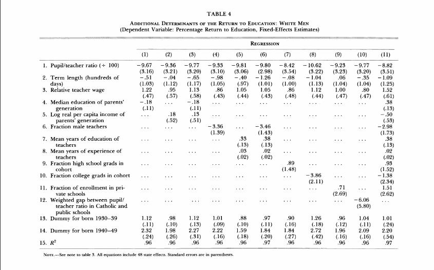
We have analyzed the effects of several other school and state-level characteristics on the returns to education. Table 4 summarizes our main findings. In each case we have included the three basic measures of school quality as well as state-specific fixed effects. To preview the results, we find that the estimated coefficients of the school quality variables are largely unaffected by the addition of controls for other characteristics, including characteristics of teachers, average income in the state, educational attainment, and characteristics of private schools.

Columns 1-3 of table 4 address the effect of family background characteristics on the return to education. A number of previous studies (including Coleman et al. [1966]) have found a strong association between family background factors, such as parental education and income, and student performance on standardized tests. If these family background characteristics are correlated with school quality and if these characteristics change substantially over time within states (SO they are not absorbed by the state fixed effects), our estimates of the effect of school quality may be confounded by the effect of family background variables.

Although the census lacks direct information on the education of individuals' parents, we can at least partially control for differences in parental education by including the median level of education among adults who lived in the state when the men in our sample attended school (row 4). Likewise, we include the log of real per capita income in the state at the time the cohorts in our sample entered school (row 5).1°Regardless of whether they are included sepa-

' O These and subsequent covariates are described in App. A.

ADDITIONAL OF THE RETURN WHITE MEN DETERMINANTS TO EDUCATION: (Dependent Variable: Percentage Return to Education, Fixed-Effects Estimates)

-

1. Pupillteacher ratio ( t 100)

2. Term length (hundreds of days)

3. Relative teacher wage

4. Median education of parents' generation

5. Log real per capita income of parents' generation

6. Fraction male teachers

7. Mean years of education of teachers

8. Mean years of experience of teachers

9. Fraction high school grads in cohort

10. Fraction college grads in cohort

11. Fraction of enrollment in private schools

12. Weighted gap between pupil1 teacher ratio in Catholic and public schools

13. Dummy for born 1930-39

14. Dummy for born 1940-49

NOTE-See note to table 3 All equations ~nclude48 slate effects Standard errors are m parentheses

JOURNAL OF POLITICAL ECONOMY *4

rately or jointly, each of these variables has a relatively small and statistically insignificant effect on the return to education. Moreover, the estimated effects of the three main school quality variables (pupil1 teacher ratio, term length, and relative teacher wage) are unaffected by the inclusion of these family background variables.

Teacher Characteristics

Columns 4-6 explore the role of teacher characteristics on the returns to schooling. The fraction of male teachers is included because, holding constant the level of teacher salaries, one might expect the quality of the teaching staff to vary with the fraction of male teachers. For example, assuming that female teachers were paid less than oth- erwise identical males during the period 1926-66, one can view the percentage of male teachers as a proxy for lower-quality teachers. Alternatively, one can view the fraction of male teachers as an indicator of higher nonwage compensation or better working conditions within the schools, which would be likely to attract relatively more men into the teaching profession, with relative wages held constant.

The results indicate that an increase in the fraction of male teachers in the state has a substantial negative impact on students' return to education. An increase in the fraction of male teachers from 19 to 42 percent, which is the range observed across states in 1966, is associated with an 0.8-percentage-point reduction in the return to years of education above the threshold. Whether the fraction of male teachers influences the return to education because males are less effective teachers, or through some other channel, is difficult to ascertain.

Columns 5 and 6 add the mean years of education of teachers in the state to the regression equation. The estimated coefficient of mean teacher education is positive and statistically significant, whereas the estimated effect of teachers' experience is negligible. No- tice that the pupillteacher ratio and relative teacher wage continue to be significant determinants of the return to education when these teacher quality variables are included; in fact, their estimated coefficients are hardly affected by the addition of the teacher quality variables. Furthermore, the addition of controls for the average education and experience of teachers hardly changes the estimated coefficient of the fraction of male teachers.

Educational Distribution

Estimates of the high school completion rate and the college completion rate for each state of birth and cohort group are included in the models in columns 8 and 9. These variables are added to control for


biases that may arise as more schooling is acquired by a higher fraction of a given cohort. For example, suppose that more schools are built in a state, leading to a decrease in the travel time for students and a reduction in the pupillteacher ratio. Suppose further that individuals differ in their expected returns to education and that as more schools are built some students with lower expected returns to education stay in school longer. In this case, one might expect increases in school quality to be correlated with lower returns to education, re- flecting a negative correlation between the average rate of return to education and the fraction of individuals with higher education. In our data there is a strong positive correlation (both in a cross section and within particular states over time) between average educational attainment and measures of education quality.11 Therefore, if rates of return vary systematically across the population and if individuals with higher expected returns choose more schooling, there is a possible downward bias in our estimates of the effect of schooling quality on returns to education. This can be controlled in part by including measures of the fraction of individuals at higher education levels in each cohort.

Neither the high school graduation rate nor the college graduation rate has a statistically significant effect on the return to education. Moreover, the high school graduation rate has a negative coefficient, and the college graduation rate has a small, positive coefficient. These results provide no evidence that students sort themselves into different education levels on the basis of different expected returns to schooling.

We have also explored the effect of the dispersion in educational attainment in a state on the return to education. As discussed further below, improvements in school quality are associated with lower dispersion in the distribution of education. Some models of ability bias in the estimated return to schooling predict that a reduction in the dispersion in the educational distribution is associated with higher returns to education. We find little support for this hypothesis in our data. For example, the standard deviation of years of education has a small and statistically insignificant ( t = -0.59) negative effect if it is added to the model in column 10 of table 3. The inclusion of this variable hardly changes the impact of the school quality variables.

Private Schools

Our measures of school quality are based on the characteristics of the public school system in each state. Not all students attend public

" For example, across our three cohorts and 49 states of birth, the correlation between the fraction who completed high school and the pupillteacher ratio is - .71.


schools, however. During the period 1920-60, the fraction of students enrolled in private schools grew from 7.5 percent to 13.6 percent. The fraction of private school enrollment also varies across states: in 1938, for example, the share of private enrollments ranged from less than 2 percent in many southern states to over 20 percent in New Hampshire and Rhode Island. The presence of private schools introduces two potential sources of unobserved variation in school quality. First, private schools may be more or less effective than public schools.12 Second, private schools may have different staffing levels, teacher salaries, and term lengths than the public schools. In an effort to examine these issues, we collected information on private school enrollments and pupillteacher ratios by state and cohort. Our information on the pupillteacher ratio in private schools is limited to Cath- olic schools, but 90 percent of private-school students attended Cath- olic schools during our sample period.

Evidence on the effect of accounting for private school enrollment is presented in columns 9 and 10 of table 4. In column 9 we include the fraction of students enrolled in all private schools as an additional explanatory variable for the rate of return to education. When pupil1 teacher ratios, term length, and relative teacher salaries in the public schools are controlled for, the coefficient of the private school enrollment variable is numerically small and statistically insignificant. These results suggest that increases in private school enrollment do not by themselves affect returns to education.

The specification in column 10 is an attempt to measure the biases created by using data for the public schools to proxy pupillteacher ratios for the state as a whole. The average pupillteacher ratio in a state is a weighted average of ratios in the public and private systems. Hence, the measurement error in using the public school ratio as a proxy for the overall state average is the product of the fraction of enrollment in private schools and the gap between the private and public school ratios.13 An estimate of this error component is included in the model in column 10. As predicted by a naive model of attenua- tion bias, the addition of this control variable raises the estimated coefficient of the pupillteacher ratio. Furthermore, the estimated coefficient of the error component is (roughly) equal to the estimated

Coleman, Hoffer, and Kilgore (1982) present data on standardized test scores that indicate higher achievement levels among students in private (mainly Catholic) schools. The interpretation of these data is an issue of some dispute: see Goldberger and Cain (1982), Murnane (1984), and San Segundo (1988).

l3 Let p represent the pupillteacher ratio for all students, p l the ratio in the public school system, p2 the ratio in the private school system, and f the fraction of enrollment in private schools. Then p = (1 - f ) . pl + f .p2. Hence p - p i = f . ( p 2 - P I ) .

RETURNS TO EDUCATION 2 7 coefficient of the pupillteacher ratio in the public schools. Neverthe- less, the relatively modest changes in the coefficients of the public school quality variables suggest that the biases introduced by measuring only the quality of public schools are small.

Up to this point we have proceeded by considering individually extensions to the basic quality variables (family background, teacher quality, educational attainment, and private schools). In column 1 1 we include several of the additional variables jointly. With the excep- tion of the term length variable, the school quality variables have their expected signs and are statistically significant. In contrast, the variables measuring family background characteristics, student educational achievement, and private school attendance generally have insignificant and small effects. The data seem to accord a greater role to school quality than to other variables in determining the return to education.

Evidence for Black and White Men Born in the South

Despite the limited evidence of family background effects in the return to education, the wide variation in school quality for men from different states and cohorts presumably reflects differences in incomes and tastes for education over time and across states. T o the extent that unmeasured differences in family incomes and tastes affect individuals' returns to education, the estimated school quality effects in tables 3 and 4 may be overstated. A potentially better test of the effects of school quality is based on the earnings experiences of blacks. The rapid improvements in school quality that occurred in the black schools of the segregated southern states between 1920 and 1960 provide an arguably exogenous experiment for studying the effects of school quality.

In a related paper (Card and Krueger 1992), we have examined the effects of school quality on the returns to education for southern- born black and white men who worked in northern cities in 1960, 1970, or 1980. Our results are qualitatively and quantitatively similar to those in tables 3 and 4. For example, the estimated coefficient of the pupillteacher ratio in a model similar to the one in column 7 of table 3 is -5.9, with a standard error of 2.39. The estimated coefficients of term length and teacher wages are also similar to those in table 3. We believe that our findings for southern-born black and white men provide additional support for a causal interpretation of the school quality effects in tables 3 and 4.


D. Adjustments for Mobility of Preschool and School-Age Children

In our analysis so far, we have implicitly assumed that an individual attends public school in his state of birth. Interstate mobility of preschool and school-age children introduces a problem similar to measurement error in the interpretation of the returns to education for individuals born in a particular state. To proceed, it is useful to concentrate on a single cohort and to assume that individuals are educated in only one state. Let yj represent the estimated rate of return to education for individuals born in state j (in a particular cohort), and let y t represent the rate of return for individuals educated in state i. Finally, let pij represent the probability that an individual attended school in state i , given that he was born in state j. Then

Let P represent a matrix whose i ,j element is p,,. Then the vector of coefficients y is related to the vector of true returns y* by y = Py*. Given estimates of y and P,one can obtain an estimate of y* by y* = P-'y.Notice that if individuals are always educated in their state of birth, then P is an identity matrix and y* = y.

We obtained an estimate of the matrix P by cross-tabulating state of birth with current state of residence for white children aged 6-12 (both male and female) in the Public-Use Sample of the 1940 census. For most states, the probability that a 6-12-year-old is living in his or her state of birth is around 90 percent, although it is lower for children born in the District of Columbia (62 percent). In principle, this estimate of the matrix P is appropriate only for children born between 1928 and 1934, and only for those with 1-6 years of schooling. Nonetheless, we used this transition matrix to transform the estimated rates of return for each of the three birth cohorts into estimates of the rate of return for attending school in different states. We then reestimated the regression models in table 3, using the corrected rates of return as dependent variables.14

The mobility-adjusted results are qualitatively similar to those in table 3. The correction has the effect of expanding the standard deviation of the estimated returns by 19 percent for the 1920-29 birth cohort, 11 percent for the 1930-39 cohort, and 8 percent for the 1940-49 cohort. As a consequence, the magnitudes of the estimated coefficients for the school quality variables are typically 5-15

l4 We also used the estimated P matrix to obtain estimated sampling variances for the corrected returns. These sampling variances were used to weight the regressions. A table containing these results is available on request.


percent larger than in the uncorrected model, although the associated standard errors rise by roughly the same proportion. On balance, the results suggest that adjustments for interstate mobility have a relatively minor impact on the qualitative and quantitative conclusions in table 3. This reflects the relatively low mobility rates of preschool and school-age children and the absence of a strong connection between interstate mobility and the geographic pattern of the measured quality of education.

E . Log-Linear SpeciJicatzon

The preceding estimates examine the relationship between school quality and the return to education for years of schooling beyond the level attained by the second percentile of the education distribution. This specification of the education variable was selected for its ability to capture the nonlinear return structure illustrated in figures 1 and 2. Compared to a conventional log-linear specification, the linear- spline specification provides a slightly better fit to the micro data: the difference in maximized log likelihoods between the spline model and a conventional linear return to education model is 99.0 for the 1920-29 cohort, 150.0 for the 1930-39 cohort, and 315.1 for the 1940-49 cohort.

Nevertheless, a log-linear specification is widely used in the literature, and it is useful to check the sensitivity of our estimates to the functional form assumptions. Consequently, we have reestimated the returns to education by state and cohort using a linear specification for education. The two sets of returns have very similar weighted means (6.42 for the spline estimates vs. 6.45 for the linear estimates) and are highly correlated (the correlation coefficient across 147 observations is .997). The close correspondence between the two sets of estimated returns is understandable, given that the spline specification differs from the linear specification for only 2 percent of the sample.

Table 5 presents estimates of the relation between our school quality measures and the returns to education derived from a log-linear specification. Except for the choice of the dependent variable, the models are the same as in table 3. The coefficient estimates in table 5 are 10-20 percent smaller than those in table 3. Regardless of specification, however, the school quality variables have statistically significant and sizable effects on the return to education. These results suggest that the relationship between school quality and the return to education is not particularly sensitive to the specification used to estimate the return to education.

I st.ZX SLC5"

RETURNS TO EDUCATION 3 l

IV. The Effects of School Quality on Education and Earnings

Our analysis of the relation between school quality and the return to education has the advantage of controlling for unobserved differences across cohort and state of birth groups. Any background factors (such as family income) that raise the earnings of individuals from a particular group are absorbed by the cohort-specific state of birth effects included in our first-stage equation. A disadvantage of concen- trating on the return to education is that changes in school quality may simply widen the distribution of earnings without raising average incomes. It is even conceivable that changes in school quality alter the distribution of schooling, and the slope of the earnings-schooling relation, with no effect on the distribution of earnings.

T o explore these issues, we proceed in two steps. First we analyze the influence of changes in school quality on the location and shape of the earnings-schooling relationship. This requires that we analyze the effect of school quality on the educational distribution (in particular, on the level of education attained by the second percentile of the distribution) and on the intercepts of the schooling-earnings relation. Second, we present some simple reduced-form evidence on the connection between school quality and the levels of education and earnings. In contrast to our analysis of the returns to education, the effects of school quality on the education distribution and on the levels of earnings cannot be identified in models that include unrestricted cohort-specific state of birth effects. This limitation should be kept in mind in interpreting the results.

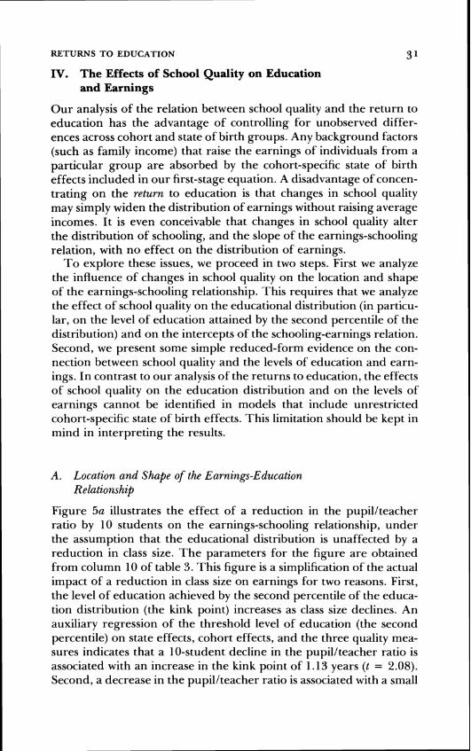
A. Location and Shape of the Earnings-Education Relationship

Figure 5a illustrates the effect of a reduction in the pupillteacher ratio by 10 students on the earnings-schooling relationship, under the assumption that the educational distribution is unaffected by a reduction in class size. The parameters for the figure are obtained from column 10 of table 3. This figure is a simplification of the actual impact of a reduction in class size on earnings for two reasons. First, the level of education achieved by the second percentile of the education distribution (the kink point) increases as class size declines. An auxiliary regression of the threshold level of education (the second percentile) on state effects, cohort effects, and the three quality measures indicates that a 10-student decline in the pupillteacher ratio is associated with an increase in the kink point of 1.13 years (t = 2.08). Second, a decrease in the pupillteacher ratio is associated with a small

JOURNAL OF POLITICAL ECONOMY

..-- base

1-

,P 0.8- . . . reduce ratio by 10

18 :::: 0.2-

0-0 4 8 12 16 20

Years of Education

b

Years of Education

FIG.5.-Effect of reducing pupillteacher ratio by 10:a, ignoring effects on intercept and education distribution; b, including effects on intercept and education distribution.

(albeit statistically insignificant) upward shift in the intercepts of the earnings-schooling relation. A regression of the state of birth-specific intercepts of the earnings-schooling relation on state of birth effects, cohort effects, and the three school quality variables yields coefficients of -0.25 (t = 0.68) for the pupillteacher ratio (divided by loo), -0.17 (t = - 1.43) for the term length variable (divided by loo), and 0.1 1 (t = 1.88) for the relative teacher wage. The quality variables are jointly insignificant (p-value = .31) in this model.

Figure 56 illustrates the effect of a 10-student reduction in the pupillteacher ratio including these additional effects. It is clear from the figure that a decrease in the pupillteacher ratio rotates and shifts out the earnings-schooling relationship, with a crossover point around the twelfth or thirteenth grade level. (In fact, when we narrow the sample to individuals who have exactly 12 years of schooling, we find that school quality has an insignificant effect on earnings, suggesting that the crossover point is around the twelfth grade.) At

RETURNS TO EDUCATION 33 a fixed level of education, individuals with postsecondary education appear to benefit from improved school quality, whereas those with less than a high school education appear to earn less. However, an increase in school quality raises schooling levels, particularly in the lower tail of the education distribution. These gains in education offset the apparent losses associated with the shift in the earnings- schooling function, leaving individuals in the lower tail of the earnings distribution approximately as well off and individuals in the mid and upper portions of the earnings distribution better off.

T o further study the effects of changes in school quality on individuals in the lower tail of the earnings distribution, we used a regression of log earnings on state of residence effects, age, age squared, marital status, and SMSA residence to compute earnings residuals within state of birth and cohort cells. We then regressed the tenth and twenty-fifth percentiles of the adjusted earnings distributions for each cell on state of birth dummies, cohort dummies, and the school quality measures. These regressions indicated small but generally positive (and marginally significant) effects of higher school quality on earnings of the tenth and twenty-fifth percentiles. There is certainly no evidence of a negative effect of school quality on the lower tail of the earnings distribution.

B. Reduced-Form Estimates

T o summarize the effect of school quality on mean earnings, we con- clude with some simple reduced-form estimates of the effect of school quality on log earnings and education. The results are presented in table 6. These reduced-form models include the school quality measures, state of residence and state of birth effects, and demo- graphic variables (age, age squared, and indicators for marital status and residence in an SMSA). Notice that education is excluded from the earnings models in columns 1-6: the estimated school quality effects therefore incorporate any effects on the level of education, as well as effects on the return to each year of schooling. We emphasize that these models are estimated using a pooled sample of men from the three 10-year birth cohorts we have analyzed throughout this paper. Unlike our earlier models, these models therefore constrain the state of birth and state of residence effects to be similar across cohorts.

The results in table 6 suggest that increases in school quality are associated with increases in both mean earnings and average years of education. When the quality variables are included individually, each is a significant determinant of earnings and average education. When the three variables are included jointly, the pattern of coefficient esti-

--

TABLE 6

~ - ------ --- --------- - - - -

Log Weekly Wage Education - - - - - - - - - - ~-- ~ - - - - - - -

VARIABLEINDEPENDENT (1) (2) (3) (4) (5) (6) (7) (8) (9) (10) --- - - --- - - - --- -- - - - - -- - -- .- --- ------- .-

Pupil/teacher ratio (l 1,000) -4.24 . . . . . . -4.15 -7.10 -4.29 -59.18 . . . . . . -59.71 (.59) (.fig) (.26) (59) (3.47) (4.00)

Term length ( + 1,000) . . . 1.20 . . . . I8 .15 .30 . . . 15.23 . . . 1.16 (.15) (.22) (.14) (.23) (1.32)

Relative teacher wage (+ 100) . . . . . . 4.77 4.48 10.93 3.49 . . . . . . 60.13 59.77 (.68) (.93) (.47) (.94) (3.96) (5.43)

50 state of residence dummies yes yes yes yes Yes no yes yes Yes Yes 48 state of birth dummies yes yes yes Yes no Yes Yes Yes Yes Yes R~ .088 ,088 .088 .088 ,085 ,075 ,100 ,100 .lo0 .lo0 p-value for F-test of quality variables . . . . . . . . . .0001 .0001 .0001 . . . . . . . . . .0001

-p -- -- - - -- - -- - - - -- - -~ -------p-----p--p-p----p---pp...-

N o , r -Each quatlon also includra age and its square, a du~nnly indicating current nrarital status, two cohort dunroriea, and a dummy indicating residence in an SMSA. Sample size ia 1,018,477. Standard rrrors are in parentheses.

RETURNS T O EDUCATION 3 5 mates is similar to the pattern we found in tables 3-5: the pupil1 teacher ratio and the relative teacher wage remain significant, and the term length variable falls to insignificance. For reference we also report two restrictive specifications of the earnings models. The model in column 5 excludes the state of birth dummies and therefore uses both within-state and between-state variation in school characteristics to estimate the school quality effects. This exclusion, which is implicit in models reported by Rizzuto and Wachtel (1980), yields much larger school quality effects. The model in column 6 includes the state of birth effects but excludes current state of residence effects. This exclusion lowers the goodness of fit of the earnings model but has little impact on the magnitude of the school quality coefficients.

According to the estimates in columns 4 and 10, a decrease in the pupillteacher ratio by 10 students is predicted to raise average earnings by 4.2 percent and raise average education by 0.6 years. In this sample the conventional return to education (i.e., the coefficient of education when it is added to the list of variables in the earnings model and the school quality variables are excluded) is 5.38 percent. Thus a 0.6-year increase in average education might be expected to increase earnings by 3.2 percent. The overall gain in earnings from a reduction in the pupillteacher ratio is therefore 30 percent bigger than would be expected on the basis of the increase in average education alone. A similar calculation for the relative teacher wage shows that a 30 percent increase in teacher wages increases average education by 0.18 years and average log wages by 1.34 percent. The gain in earnings is roughly 40 percent bigger than would be expected on the basis of the increase in education alone.

We have also used the 1970 census to estimate reduced-form equations similar to the ones in table 6 for a sample of white men born in 1913-39. The results are comparable, although the effects of the relative teacher wage variable on mean earnings for the 1970 sample are smaller and statistically insignificant (except when the state of birth effects are excluded from the model). The coefficient of the pupillteacher variable on mean earnings is larger in 1970 than in 1980, whereas the coefficients of the quality variables on mean education are uniformly smaller. However, the 1970 sample is substantially smaller (378,000 vs. 1,018,000 in 1980) and the sampling errors are large enough that few of these differences are highly significant.

We draw two conclusions from the reduced-form relations between earnings, education, and school quality. First, increases in school quality during the past century are associated with increases in years of schooling and average wages. Second, the increases in earnings appear to reflect both a gain for the added years of education and


an increase in the return for each existing year of education. Both conclusions should be tempered by our inability to control for unobserved cohort-specific factors that may raise the earnings of individuals from states with better schools in the reduced-form models. When these conclusions are taken together with the evidence we have assembled on the returns to education, however, we believe that there is strong support for the conclusion that increases in school quality lead to higher earnings.

V. Conclusion and Discussion

The estimates presented in this paper provide new evidence that the quality of schooling affects earnings. Men who are educated in states with higher-quality school systems earn higher economic returns for their years of schooling. Although the evidence is necessarily nonex- perimental, we believe that our findings are consistent with a causal interpretation of the role of school quality. In the first place, our findings are based on statistical models that control for any differences across state of birth and cohort groups in the overall level of earnings. Second, we have controlled for differences in the rates of return to education earned by current residents in different regions of the country. Third, we have controlled for any permanent differences across states in the return to education earned by different cohorts of men and for differences in family background measures (education and earnings of the parents' generation) that may affect subsequent labor market performance. Finally, our reduced-form analysis confirms that increases in school quality increase the average earnings of students. Thus the effects of school quality are not simply redistributive, nor are they an artifact of changes in the distribution of schooling attainments.

Our findings underscore the paradox we noted in the Introduc- tion: school quality appears to have an important effect on labor market performance but is widely believed to have no impact on standardized achievement tests. We note, however, that two recent experimental studies of school characteristics and test scores are con-sistent with positive school quality effects. A large-scale randomized study of class sizes in Tennessee suggests that reductions in the pupil/ teacher ratio for elementary school students significantly increase test scores on reading and math exams (see Finn and Achilles 1990). Another recent randomized study finds that lengthening the school term by providing extra instruction during the summer has a positive effect on disadvantaged students' test scores (see Sipe, Grossman, and Milliner 1988). Although more work is needed to resolve the available

37 RETURNS T O EDUCATION

evidence, we believe that success in the labor market is at least as important a yardstick for measuring the performance of the education system as success on standardized tests. At a minimum, our finding of a positive link between school quality and the economic returns to education should give pause to those who argue that investments in the public school system have no benefits for students.

Appendix A

Data Sources

A. Basic Data on School Quality

The following series were extracted from various issues of the Biennial Suruey of Education and the Digest of Education Statistics: (a) the number of pupils enrolled in full-time public elementary and secondary schools; (b) the average number of days in the school term (full-time public elementary and secondary schools); (c) the average number of days attended by each enrolled student (full-time public elementary and secondary schools) (1920-58 only); (d) the number of instructional staff, including supervisors and principals (full-time public elementary and secondary schools); (e) the percentage of teachers who are male (full-time public elementary and secondary schools); and ( f ) the average annual salary per member of the instructional staff (full-time public elementary and secondary schools).

These data were collected by state for alternating years, beginning with 1919-20. In some cases, the figures in the most recently published Biennial Survey were revised in subsequent editions. We have attempted to incorporate as many of these revisions as possible. For 1960 and later we collected a variable representing the percentage of school days attended by enrolled students. This percentage was then used to construct an estimate of average days attended from the series on the length of the school term. The data from the biennial editions of the survey are allocated to the previous two years: for example, data from the 1937-38 edition are used for both 1937 and 1938.

B. Construction of the Relative Teacher Wage

Two wage series were combined to create a relative wage index for teachers in each state. For 1920-38, we used the wage paid to laborers on federal road construction projects. This wage is available on a regional basis (for nine census regions) in the Statistical Abstract of the United States. Data for 1920-29 are taken from the 1930 edition, table 358. Data for 1930-56 are taken from the 1957 edition, table 271. For 1940-66, we use the average state-level wage of workers covered by the social security system, from U.S. Department of Labor Employment and Training Administration Handbook Number 394. To convert the regional construction wage rates into state-level averages, we formed the average ratio of the state social security wage to the regional construction wage in the period 1940-44. This average ratio was then applied to the construction wage in the period 1920-38 to obtain a state-specific average.

3t3 JOURNAL OF POLITICAL ECONOMY

C. Data on Education and Experience of Teachers

We used the Public-Use Sample of the 1940 census to form extracts of teachers in each of the 48 (mainland) states and District of Columbia. Teachers were identified by industry (educational services) and occupation (teachers not elsewhere classified). We sampled only those teachers who reported either white or black race and who reported positive earnings and weeks worked and nonallocated age, sex, race, industry, occupation, and years of education. The extract contains 9,16 1 teachers.

We used the Public-Use Sample of the 1950 census to form extracts of teachers in each of the 48 (mainland) states and District of Columbia. (Owing to technical difficulties, our Public-Use Sample excludes one-eighth of the available sample.) Teachers were identified by industry (educational services) and occupation (teachers not elsewhere classified). We sampled only those teachers who reported either white or black race and who reported nonallocated age, sex, race, industry, occupation, and years of education. The extract contains 3,206 teachers.

We used the Public-Use Sample of the 1960 census to form extracts of teachers in each of the 48 (mainland) states and District of Columbia. Teachers were identified by industry (educational services) and occupation (elementary school teachers and secondary school teachers). We sampled only those teachers who reported either white or black race and who reported nonallocated age. The extract contains 16,052 teachers.

D. Data on Family Background

1. Average Per Capita Income

We collected average personal income per capita by state for the years 1930, 1940, and 1950 from State Personal Income: Estimates for 1929-1 982, Revised Estimates (Bureau of Economic Analysis, 1984). The income data were originally derived from the National Income and Product Accounts. The con- sumer price index was used to convert the data into real dollars. The state- level per capita income in 1930 was assigned to the cohort of men born in the 1920s, the state-level per capita income in 1940 was assigned to the cohort of men born in the 1930s, and the state-level per capita income in 1950 was assigned to the cohort of men born in the 1940s. These years roughly correspond to the years in which educational expenditures for each cohort would have been determined.

2. Median Education of Parents' Generation

As a measure of the education of each cohort's parents, we collected information on the median education of white persons aged 25 or older by state in 1940, 1950, and 1960. These data are reported in Statistical Abstract of the United States (nos. 66, 75, 85) and were originally derived from the 1940,

RETURNS T O EDUCATION 39 1950, and 1960 censuses. In 1940, the education data are reported only for native-born individuals, and in 1950 and 1960 the data pertain to native and foreign-born individuals. The median education of adults in 1940 was assigned to the 1920s cohort, the median education of adults in 1950 was assigned to the 1930s cohort, and the median education of adults in 1960 was assigned to the 1940s cohort.

E. Private Schools

State-level data on the number of students enrolled in private schools, the number of students enrolled in Catholic schools, and the number of teachers in Catholic schools were collected from the Biennial Suroey. Unfortunately, these variables are available only on an irregular basis. Data for 1937-38 were assigned to the cohort born in the 1920s, data for 1949-50 were assigned to the cohort born in the 1930s, and data for 1955-56 were assigned to the cohort born in the 1940s.

Appendix B

1980 Micro Data Samples

Our samples are taken from the Public-Use A Sample of the 1980 census (a 5 percent sample of the population). The samples consist of men born in the 48 mainland states o r the District of Columbia between 1920 and 1949 and currently living in any of the 50 states or District of Columbia. Year of birth is estimated from information on age and quarter of birth. We include only those individuals whose race is identified as "white." Individuals with imputed information on age, race, sex, education, weeks worked, or total annual earnings are excluded, as are individuals who report no weeks of work in 1979. In addition, individuals with wage or salary income in 1979 less than $101 and those with average weekly wage and salary income of less than $36 or greater than $2,500 are excluded. The final sample sizes are 279,008 for those born in 1920-29,299,063 for those born in 1930-39, and 441,675 for those born in 1940-49. These samples are used to form the first-stage estimates of the returns to education in our two-step procedure and the reduced-form estimates presented in table 6.

References

Behrman, Jere R., and Birdsall, Nancy. "The Quality of Schooling: Quantity Alone Is Misleading." A.E.R. 73 (December 1983): 928-46.

Card, David, and Krueger, Alan. "School Quality and Black-White Relative Earnings: A Direct Assessment." Q.J.E. 107 (February 1992).

Chiswick, Barry R. Income Inequality: Regional Analyses within a Human Capital Framework. New York: Columbia Univ. Press (for NBER), 1974.

Coleman, James S., et al. Equality ofEducationa1 Opportunity. Washington: Gov- ernment Printing Office, 1966.

Coleman, James S.; Hoffer, Thomas; and Kilgore, Sally. High School Achieue- ment: Public, Catholic, and Private Schools Compared. New York: Basic Books, 1982.

4 O JOURNAL OF POLITICAL ECONOMY

Finn, Jeremy D., and Achilles, Charles M. "Answers and Questions about Class Size: A Statewide Experiment." American Educ. Res. J . 27 (Fall 1990): 557-77.

Freeman, Richard. Black Elite: The New Marketfor Highly Educated Black Ameri- cam. New York: McGraw-Hill, 1976.

Goldberger, Arthur S., and Cain, Glen G. "The Causal Analysis of Cognitive Outcomes in the Coleman, Hoffer and Kilgore Report." Sociology Educ. 55 (April/July 1982): 103-22.

Griliches, Zvi. "Economic Data Issues." In Handbook of Econometrics, vol. 3, edited by Zvi Griliches and Michael D. Intriligator. New York: North- Holland, 1986.

Griliches, Zvi, and Mason, William M. "Education, Income, and Ability." J.P.E. 80, no. 3, pt. 2 (May/June 1972): S74-S103.

Hanushek, Eric A. "The Economics of Schooling: Production and Efficiency in Public Schools." J . Econ. Literature 24 (September 1986): 1141-77.

Heckman, James J., and Polachek, Solomon. "Empirical Evidence on the Functional Form of the Earnings-Schooling Relationship." J . American Statis. Assoc. 69 (June 1974): 350-54.

Johnson, George E., and Stafford, Frank P. "Social Returns to Quantity and Quality of Schooling." J . Human Resources 8 (Spring 1973): 139-55.

Morgan, James N., and Sirageldin, Ismail. "A Note on the Quality Dimension in Education." J.P.E. 76 (SeptemberIOctober 1968): 1069-77.

Murnane, Richard J. "A Review Essay-Comparisons of Public and Private Schools: Lessons from the Uproar." J . Human Resources 19 (Spring 1984): 263-77.

Rizzuto, Ronald, and Wachtel, Paul. "Further Evidence on the Returns to School Quality." J . Human Resources 15 (Spring 1980): 240-54.

San Segundo, Maria Jesus. "Do Private Schools Make a Difference?" Working paper, Southern European Economics Discussion Series. Leioa, Vizcaya, Spain: Inst. Economia Publica, August 1988.

Sipe, Cynthia L.; Grossman, Jean Baldwin; and Milliner, Julita A. Summer Training and Education Program (STEP): Report on the 1987 Experience. Phila-delphia: PublicIPrivate Ventures, 1988.

Smith, James P., and Welch, Finis. "Black Economic Progress after Myrdal." J . Econ. Literature 27 (June 1989): 519-64.

Wachtel, Paul. "The Effects on Earnings of School and College Investment Expenditures." Rev. Econ. and Statis. 58 (August 1976): 326-31.

Welch, Finis. "Measurement of the Quality of Schooling." A.E.R. Papers and Proc. 56 (May 1966): 379-92.

. "Labor-Market Discrimination: An Interpretation of Income Differ- ences in the Rural South." J.P.E. 75 (June 1967): 225-40.

. "Black-White Differences in Returns to Schooling." A.E.R. 63 (De- cember 1973): 893-907. (a)

. "Education and Racial Discrimination." In Discrimination in Labor Markets, edited by Orley Ashenfelter and Albert Rees. Princeton, N.J.: Princeton Univ. Press, 1973. (b)

does school quality matter? returns to education and...

Documents