Documentation for: icaeyeblinkmetrics() Version 3.2

This EEGLAB toolbox is designed for automated/semi-automated selection of ICA components associated with eye-

blink artifact using time-domain measures. The toolbox is based on the premises that 1) an ICA component

associated with eye blinks should be more related to the recorded eye blink activity than other ICA components,

and 2) removal of the ICA component associated with eye blinks should reduce the eye blink artifact present within

the EEG following back projection.

Other than the EEG input, the only required input for the function is specification of the channel that exhibits the

artifact (in most cases the VEOG electrode). This can either be stored within the EEG.data matrix or within

EEG.skipchannels. It will then identify eye-blinks within the channel to be used for computation of the metrics listed

below. If you are not sure what channel to choose, you can let the function determine the channel where the

artifact maximally presents but this does slow the function down.

The toolbox does not change the data in any way, it only provides an output stored in ‘EEG.icaquant’ providing:

1. Metrics:

a. The correlation between the measured artifact in the artifact channel and each ICA component. (i.e.

how similar the ICA component is to the eye blink)

b. The adjusted normalized convolution of the ICA component activity with the measured artifact in the

artifact channel. (i.e., how well does the ICA component overlap with the eye blink)

c. The percent reduction in the artifact present in the EEG for each ICA component if it was removed.

(i.e., how much is the eye blink artifact reduced in the EEG when the component is removed)

2. Identified Components: the ICA components that exhibit statistically significant values for all three metrics.

Alpha defaults to p ≤ 0.001.

3. Artifact Latencies: the latencies that were used in the computation of the metrics.

Release Notes:

Version 3.0

Updated eyeblinklatencies() code to increase computational speed. Default threshold was lowered to correlation of 0.96

based upon updates to the implementation approach. Added parameter to allow for inputting a user specified template

for eye blink identification. For older Matlab versions, that may not allow for the new approach, the old implementation

is retained.

Updated icablinkmetrics() code to increase computational speed. Added catch to reduce correlation threshold for

eyeblinklatencies() to 0.9 if too few eye blinks are identified. Reduced the volume of content written to the Matlab

window.

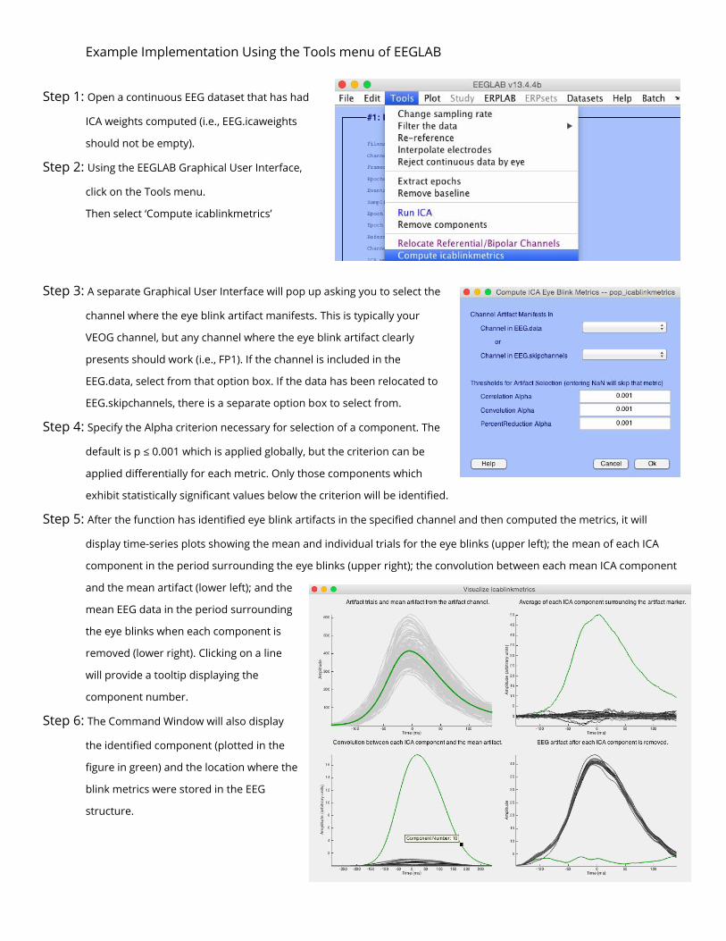
Example Implementation Using the Tools menu of EEGLAB

Step 1: Open a continuous EEG dataset that has had

ICA weights computed (i.e., EEG.icaweights

should not be empty).

Step 2: Using the EEGLAB Graphical User Interface,

click on the Tools menu.

Then select ‘Compute icablinkmetrics’

Step 3: A separate Graphical User Interface will pop up asking you to select the

channel where the eye blink artifact manifests. This is typically your

VEOG channel, but any channel where the eye blink artifact clearly

presents should work (i.e., FP1). If the channel is included in the

EEG.data, select from that option box. If the data has been relocated to

EEG.skipchannels, there is a separate option box to select from.

Step 4: Specify the Alpha criterion necessary for selection of a component. The

default is p ≤ 0.001 which is applied globally, but the criterion can be

applied differentially for each metric. Only those components which

exhibit statistically significant values below the criterion will be identified.

Step 5: After the function has identified eye blink artifacts in the specified channel and then computed the metrics, it will

display time-series plots showing the mean and individual trials for the eye blinks (upper left); the mean of each ICA

component in the period surrounding the eye blinks (upper right); the convolution between each mean ICA component

and the mean artifact (lower left); and the

mean EEG data in the period surrounding

the eye blinks when each component is

removed (lower right). Clicking on a line

will provide a tooltip displaying the

component number.

Step 6: The Command Window will also display

the identified component (plotted in the

figure in green) and the location where the

blink metrics were stored in the EEG

structure.

Example Implementation Code Using Command Window

clear; clc; % Clear memory and the command window

eeglab; % Start eeglab: Requires Matlab Signal Processing Toolbox & Statistics Toolbox

filelocation = '/Studies/'; % Establish path to where the SET file is located

%% Prepare Data for ICA computation

% Read in a continuous EEG dataset with any bad channels/segments removed

EEG = pop_loadset('filename','RawEEG.set','filepath',filelocation); EEG = eeg_checkset(EEG);

% Remove additional data points 2 seconds outside of triggers

winPadding = 2;

winStart = (EEG.event(1).latency-(EEG.srate*((1000/EEG.srate)*winPadding)));

winStop = (EEG.event(end).latency+(EEG.srate*((1000/EEG.srate)*winPadding)));

if (winStart < 1); winStart = 1; end; if (winStop > EEG.pnts); winStop = EEG.pnts; end;

EEG = pop_select( EEG, 'point', [winStart, winStop]); EEG = eeg_checkset(EEG);

% HighPass Filter the data to remove slow drift

EEG = pop_basicfilter(EEG,1:size(EEG.chanlocs,2),'Filter','highpass',...

'Design','butter','Cutoff',0.05,'Order',2,'Boundary',87);

% Relocate referential/bipolar channels so they can be recovered later if necessary

EEG = movechannels(EEG,'Location','skipchannels','Direction','Remove',...

'Channels',{'M1','M2','VEOG','HEOG'});

% Compute ICA

EEG = pop_runica(EEG, 'icatype', 'runica', 'options', ...

{'extended',1,'block',floor(sqrt(EEG.pnts/3)),'anneal',0.98});

EEG = eeg_checkset(EEG);

%% icablinkmetrics implementation

% Find Eye Blink Component(s)

EEG.icaquant = icablinkmetrics(EEG,'ArtifactChannel', ...

EEG.skipchannels.data(find(strcmp({EEG.skipchannels.labels},'VEOG')),:),'VisualizeData','True');

disp('ICA Metrics are located in: EEG.icaquant.metrics')

disp('Selected ICA component(s) are located in: EEG.icaquant.identifiedcomponents')

[~,index] = sortrows([EEG.icaquant.metrics.convolution].');

EEG.icaquant.metrics = EEG.icaquant.metrics(index(end:-1:1)); clear index

% Remove Artifact ICA component(s)

EEG = pop_subcomp(EEG,EEG.icaquant.identifiedcomponents,0);

Evaluating the efficacy of fully automated approaches for the

selection of eyeblink ICA components

MATTHEW B. PONTIFEX ,a VLADIMIR MISKOVIC,b AND SARAH LASZLOb

aDepartment of Kinesiology, Michigan State University, East Lansing, Michigan, USAbDepartment of Psychology, Binghamton University, Vestal, New York, USA

Abstract

Independent component analysis (ICA) offers a powerful approach for the isolation and removal of eyeblink artifacts

from EEG signals. Manual identification of the eyeblink ICA component by inspection of scalp map projections,

however, is prone to error, particularly when nonartifactual components exhibit topographic distributions similar to the

blink. The aim of the present investigation was to determine the extent to which automated approaches for selecting

eyeblink-related ICA components could be utilized to replace manual selection. We evaluated popular blink selection

methods relying on spatial features (EyeCatch), combined stereotypical spatial and temporal features (ADJUST), and a

novel method relying on time series features alone (icablinkmetrics) using both simulated and real EEG data. The

results of this investigation suggest that all three methods of automatic component selection are able to accurately

identify eyeblink-related ICA components at or above the level of trained human observers. However, icablinkmetrics,

in particular, appears to provide an effective means of automating ICA artifact rejection while at the same time

eliminating human errors inevitable during manual component selection and false positive component identifications

common in other automated approaches. Based upon these findings, best practices for (a) identifying artifactual

components via automated means, and (b) reducing the accidental removal of signal-related ICA components are

discussed.

Descriptors: Independent component analysis, EEG artifact, EEGLAB

Over the past decade, an increasing number of laboratories have

begun to utilize temporal independent component analysis (ICA) to

isolate and remove eyeblink artifacts from EEG signals. Indeed,

examination of the journal Psychophysiology over the past 2 years

reveals that nearly the same proportion of EEG investigations uti-

lize temporal ICA approaches for eyeblink artifact reduction/cor-

rection as those investigations that utilize regression-based

approaches. This is undoubtedly related in some part to the grow-

ing adoption of EEGLAB (Delorme & Makeig, 2004), a MAT-

LAB/octave-based graphical toolbox for data processing that

implements temporal ICA in its standard workflow. Of practical

importance, this temporal ICA approach to artifact correction may

not be globally appropriate for all artifacts—such as saccadic eye

movements and nonstationary artifacts, (see Hoffmann & Falken-

stein, 2008, for further discussion). However, for eyeblink artifact

correction, the ICA approach has been found to exhibit superior

performance relative to regression-based approaches (Jung et al.,

2000). An important distinction to make, however, is that, unlike

regression-based approaches, ICA does not inherently perform any

form of artifact correction. That is, these approaches are simply

blind-source signal separation techniques that attempt to dissociate

temporally independent yet spatially fixed components (Bell & Sej-

nowski, 1995). Thus, a critical limitation of temporal ICA-based

approaches to artifact correction is the reliance on subjective

human judgments to determine what components are associated

with noise rather than signal, so that the data can be back-projected

to reconstruct EEG signals in the absence of artifactual activity.

Although automated approaches exist, we have little understanding

of the extent to which these automated ICA component selection

approaches are robust to variation in signal-to-noise ratio or across

varying electrode densities. Thus, the aim of the present investiga-

tion was to determine if fully automated approaches for selecting

eyeblink-related ICA components can and should be utilized to

replace manual selection of eyeblink artifact components by human

users.

In a common EEGLAB workflow, following separation of the

signals using standard ICA algorithms, a human observer must

visually sift through the full set of temporal ICA components in

order to manually select one or more components for removal.

Such an approach is not only labor intensive, but it is also user

dependent, making it more prone to errors or, potentially, to bias

(e.g., quality control is dependent on the user’s expertise level).

Support for the preparation of this manuscript was provided by a grantfrom the Eunice Kennedy Shriver National Institute of Child Health andHuman Development (NICHD) to MBP (R21 HD078566), and by grantsfrom the National Science Foundation (NSF) to SL (NSF CAREER-1252975, NSF TWC SBE-1422417, and NSF TWC SBE-1564046).

Address correspondence to: Matthew B. Pontifex, Ph.D., Departmentof Kinesiology, 27P IM Sports Circle, Michigan State University, EastLansing, MI 48824-1049, USA. E-mail: pontifex@msu.edu

780

Psychophysiology, 54 (2017), 780–791. Wiley Periodicals, Inc. Printed in the USA.Copyright VC 2017 Society for Psychophysiological ResearchDOI: 10.1111/psyp.12827

Human fallibility is especially relevant in the case of experiments

concerned with frontal ERP/EEG activity, where it is particularly dif-

ficult to differentiate the scalp projection of the temporal ICA com-

ponent(s) associated with eyeblink activity from the scalp projection

of the temporal ICA component(s) associated with genuine, frontally

maximal cortical activity, such as the LAN (left anterior negativity;

Castellanos & Makarov, 2006). Although it is possible to inform

these decisions by inspecting temporal ICA activations (see Figure 1),

such approaches are not explicitly detailed within the EEGLAB

documentation, rendering knowledge and implementation of such

methodologies potentially variable across research laboratories.

To address the potential limitations of human-selected ICA arti-

fact rejection, a number of methods for automatic identification of

artifact-related temporal ICA components have been developed for

EEGLAB. These include ADJUST (Mognon, Jovicich, Bruzzone,

& Buiatti, 2011), CORRMAP (Viola, Thorne, Edmonds, Schneider,

& Eichele, 2009), and EyeCatch (Bigdely-Shamlo, Kreutz-Delgado,

Kothe, & Makeig, 2013). It should be pointed out that such

approaches are simply added on following the application of ICA to

the data in order to automate the selection of artifact-related compo-

nents, and are not used as a replacement for the ICA application.

The most widely downloaded software plugin is the ADJUST meth-

od, which attempts to identify a wide array of potential sources of

artifact such as eyeblinks, eye movements, cardiac-induced artifacts,

and other stereotypical movements. To this end, temporal indepen-

dent components are characterized by combining both spatial and

temporal information, with the identification of artifactual compo-

nents based on stereotyped spatiotemporal features such as temporal

kurtosis and the spatial average difference. Alternatively, the Eye-

Catch plugin attempts to distinguish temporal ICA components

based on the correlation between the scalp map projection for each

ICA component and a database of 3,452 (as of the writing of this

manuscript) exemplar eye activity-related template scalp maps. This

approach has been found to exhibit overall performance similar to

the CORRMAP function (Viola et al., 2009) but has an advantage

over CORRMAP in that it is fully automated.

A limitation of the approaches mentioned above is that they

largely rely on ancillary indices of ICA components, such as scalp

map projections of temporal ICA weights, to differentiate

eyeblink-related components from nonblink-related components,

rendering them prone to the same potential sources of error as the

human visual inspection approach—particularly when nonartifac-

tual frontally maximal ICA components occur. Since these

approaches rely on the scalp topography of the temporal ICA com-

ponents, the eyeblink component can easily be confused with

nonartifactual frontally distributed components. This is a funda-

mental weakness of any topography-based approach to selecting

the eyeblink-related temporal ICA component. In contrast, a time-

domain approach should not be vulnerable to potential confusion

between frontally distributed nonartifact components and eyeblink-

related components. Accordingly, we were interested in comparing

a time-domain approach to the existing spatial approaches. Conse-

quently, we developed a time-domain approach, icablinkmetrics,

predicated on two basic premises: (1) that the temporal ICA com-

ponent(s) associated with eyeblinks should be related to the eye-

blink activity present within the EEG more so than any other

temporal ICA component (e.g., via correlation and convolution),

and (2) that removal of the temporal ICA component associated

with the eyeblinks should reduce the eyeblink artifact present with-

in the EEG data more so than the removal of any other temporal

ICA component following back projection (when the data is recon-

structed without the artifactual component). Again, this approach is

simply added on following the application of ICA to the data in

order to automate the selection of artifact-related components, and

is not used as a replacement to the ICA application. For a more

detailed description of the background and theory underlying the

premises that guided the development of the icablinkmetrics time-

domain approach, see the online supporting information Appendix

S1. In the interest of transparency, we note that the icablinkmetrics

approach was created by author MBP with input from SL. The ica-

blinkmetrics EEGLAB plugin—which can be run from either the

command line or the Tools menu of EEGLAB—is available

through the EEGLAB Extension Manager or by downloading from

http://sccn.ucsd.edu/wiki/EEGLAB_Extensions.

The aim of the present investigation was to assess the efficacy

of these automated approaches for the selection of eyeblink-related

artifact components. To this end, we evaluated the relative merits

of automatic approaches to eyeblink component selection methods

relying on time series data (icablinkmetrics) as compared to those

relying on combined stereotypical spatial and temporal features

(ADJUST, Mognon et al., 2011) or spatial features alone (Eye-

Catch, Bigdely-Shamlo et al., 2013). An intrinsic weakness of a

temporal approach to eyeblink-related component selection is that,

with increasing noise in the time series, procedures for identifying

when eyeblink-related activity occurs are more prone to failure. To

examine this issue, we utilized simulated EEG data to investigate

the extent to which each of these automated approaches would be

sensitive to variation in the magnitude of the eyeblink artifact amid

increasing levels of noise in the signal. Next, we assessed the gen-

eralizability of these automated approaches across real EEG data

collected with varying electrode densities and in response to differ-

ent tasks. Finally, for comparison, we assessed the accuracy of the

current common method of trained observers visually selecting

temporal ICA components. Collectively, these analyses serve to

address the critical question of whether fully automated approaches

for selecting eyeblink-related ICA components can and should be

utilized to replace manual selection of eye artifact components by

human users and, if so, what their potential vulnerabilities are.

Simulated EEG Varying in the Magnitude of the Artifact

and Level of Noise

Method

A total of 3,072 simulated EEG data sets was created matched to

three (real) exemplar EEG data sets (1,024 simulations per exem-

plar data set). For each exemplar data set, simulated data were

Figure 1. Illustration of eyeblinks recorded from the VEOG electrode,

how they manifest across three midline electrode sites, and how the

eyeblink-related signal is separated from other signals using ICA

decomposition. Note the high degree of similarity between the VEOG

electrode and ICA component 1.

Eyeblink component identification 781

created representing a wide range of possible eyeblink artifact mag-

nitude and noise conditions. In this context, the aim was not to sim-

ulate the computational processes by which the EEG signal is

actually created in the brain (e.g., Laszlo & Armstrong, 2014; Las-

zlo & Plaut, 2012). Rather, our goal was to ensure that the artificial

data exhibited the same frequency domain properties and signal-to-

noise ratio (prior to the injection of more noise per the experimental

manipulations) in the same amplitude range as true EEG data. Such

an approach enabled the creation of EEG data sets that had similar

properties to real EEG, while allowing for the ability to modulate

the level of noise present within the signal as a function of the vari-

ability found within real EEG data sets. Simulated EEG data sets

were created by (1) Fourier decomposing each exemplar data set at

each channel, and then (2) producing weighted sums of sines with

random phase shifts that resulted in simulated data sets with the

same frequency characteristics as the exemplar. The first and last

100 points of the simulated time series were removed to account for

edge artifacts from the finite sum of sines, and simulated time series

were scaled to have the same mean and standard deviation as the

exemplar data sets, per channel. Each simulated data set contained

25,480 points for each of 28 channels, allowing 32.5 data points for

each ICA weight (data points/channels2). Noise was added to the

simulated data sets by randomly perturbing both the phase and

amplitude at each point in the time series. Phase perturbations were

distributed uniformly; amplitude perturbations were distributed nor-

mally. The noise perturbations within the simulated EEG data were

scaled to create 32 levels of noise ranging from 0.4 to 10 times the

standard deviation of the exemplar EEG data set in increments of

0.31 standard deviations. Simulated data constructed in this manner

do not include eyeblink artifacts, and thus constitute the “ground

truth” for ICA artifact correction. That is, this data can be compared

with reconstructed data created by removing each ICA component.

The reconstructed data that is most similar to the ground truth data

must then reflect removal of the truly artifactual eyeblink compo-

nent (as opposed to the other nonartifactual components).

Eyeblink artifacts were then introduced into the simulated data

using a Chebyshev window (250 ms in length) as the model eye-

blink. Twenty eyeblinks were introduced into the simulated time

series at a rate of roughly one blink every 1.25 s with the propaga-

tion of the simulated blinks across the scalp controlled by a spheri-

cal head model derived empirically from the exemplar EEG data

set. The simulated eyeblinks were scaled to create 32 levels of arti-

fact magnitude ranging from 20 to 300 mV in increments of 9 mV.

This approach therefore allowed for the examination of the auto-

mated eyeblink component selection algorithms across an extreme

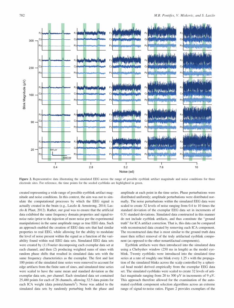
range of signal-to-noise ratios. Figure 2 provides exemplars of the

Figure 2. Representative data illustrating the simulated EEG across the range of possible eyeblink artifact magnitude and noise conditions for three

electrode sites. For reference, the time points for the seeded eyeblinks are highlighted in green.

782 M.B. Pontifex, V. Miskovic, and S. Laszlo

simulated EEG across the range of possible eyeblink artifact mag-

nitude and noise conditions.

Following each simulation, ICA decompositions were performed

using the extended infomax algorithm to extract sub-Gaussian com-

ponents using the default settings called for the binary instance

of this function in EEGLAB. To identify the components related to

the simulated artifact, the mean difference (as an absolute value)

between the blink-free simulated data and the reconstructed simulat-

ed data was computed following back projection of the data without

each ICA component, separately. As the eyeblink component(s)

should be rare relative to the other components, the truly artifactual

components were selected by normalizing the differences and com-

puting the probability of the difference occurring given a normal

distribution (see Figure 3). Those components with a probability

less than 0.05 were identified as truly artifactual components.

Across the 3,072 simulations, the truly artifactual ICA component

was identified in 1,700 (55.3%) of the simulations with instances

where the truly artifactual component was unable to be determined

occurring when the magnitude of the noise far exceeded the magni-

tude of the eyeblink (see Figure 2 and 4). Comparison of the

Figure 3. Representative data illustrating how the ground truth artifact-related ICA component was identified in the simulated EEG data. Only the

removal of a single component returns the simulated data to near its uncontaminated state, with the normalized difference between the uncontaminated

data and the contaminated data following removal of the ICA component reflecting that component as an outlier. As most components should be unre-

lated to the artifact, any component identified as an outlier was considered as related to the artifact.

Figure 4. Graphic illustration of the results of 3,072 simulations of EEG data (1,024 simulations per exemplar data set) for the likelihood of identify-

ing the artifact (sensitivity) and the likelihood of misidentifying signal as artifact (1-specificity) as a function of eyeblink magnitude and noise for

each automated procedure. As each exemplar data set was used to test the full range of signal to noise, some data points may only reflect a singular

simulation whereas others may reflect the result of three simulations at that eyeblink magnitude and noise level. Areas where the ground truth eye-

blink component was unable to be determined (occurring in 1,372 of the 3,072) are uncolored.

Eyeblink component identification 783

automated component selection procedures was restricted to only

those simulations where the truly artifactual component was able to

be identified.

Each of the three automated procedures (icablinkmetrics ver-

sion 3.1, ADJUST version 1.1.1, and EyeCatch) was then tested

using their default parameters. The icablinkmetrics function was

run using the vertical electrooculogram (VEOG) channel of the

simulated data set as the artifact comparison channel. The icablink-

metrics function identified eyeblinks within the artifact channel by

cross-correlating a canonical eyeblink waveform using the eyeblin-

klatencies function, only accepting seeded eyeblinks that exhibited

correlations of 0.96 or higher. Quantification of the efficacy of the

automated component selection approaches for reducing the simu-

lated artifact was performed by computing the percent reduction in

the difference between the blink-free simulated data and the recon-

structed simulated data ([absolute value([difference between data

with simulated eyeblink and blink-free data] 2 [difference between

reconstructed data following artifact removal and blink-free data])/

(difference between data with simulated eyeblink and blink-free

data)]; see Table 1). Perfect reconstruction of the simulated data to

its blink-free state would thus be reflected by 100% reduction

in the difference between the blink-free simulated data and the

reconstructed simulated data following artifact removal. All data

processing was conducted using an Apple iMac with a 3.5 GHz

Intel Core i7 processor and 32 GB of 1600 MHz DDR3 SDRAM.

Statistical Analysis

The efficacy of the automated procedures for identifying the eye-

blink ICA component were examined statistically by evaluating

their sensitivity (the likelihood of correctly identifying the eyeblink

ICA component(s); i.e., hits) and specificity (the likelihood of cor-

rectly not identifying a nonblink component as an eyeblink ICA

component(s); i.e., correct rejections) relative to the truly artifactu-

al component. As all simulated data sets were contaminated by eye-

blink artifact, failure to select an eyeblink component was

considered a false negative error (miss), unless the truly artifactual

component was unable to be determined (e.g., such as if the info-

max algorithm was unable to separate the seeded eyeblink from the

background noise).

Results

Component selection counts along with the sensitivity and specific-

ity are provided in Table 1. A graphic illustration of the likelihood

of identifying the artifact (sensitivity) and the likelihood of

Table 1. ICA Component Classifications

Truepositive

Truenegative

Falsepositive

Falsenegative

Sensitivity SpecificityReductionof artifact

Eyeblinkcorrectlyclassified

Nonblinkcorrectlyclassified

Said it waseyeblink but

it was not

Said it wasnot an eyeblink

but it was TP/(TP 1 FN) TN/(TN 1 FP)(Rejectedartifact)

(Retainedsignal)

(Rejectedsignal)

(Retainedartifact)

(Identifyartifact)

(Identifysignal)

Based oncomponents

selected

Simulated dataicablinkmetrics 1,234 45,900 0 466 72.6% 100% 89.5%ADJUST 1,662 45,436 464 38 97.8% 99.0% 82.8%EyeCatch 1,560 45,428 472 140 91.8% 99.0% 83.9%

Real dataicablinkmetrics 92 4,936 0 0 100% 100% 88.0%

32-channel array 40 998 0 0 100% 100% 93.4%64-channel array 38 2,233 0 0 100% 100% 89.3%128-channel array 14 1,705 0 0 100% 100% 69.2%

ADJUST 89 4,738 198 3 96.7% 96.0% 86.6%32-channel array 39 959 39 1 97.5% 96.1% 91.3%64-channel array 38 2,110 123 0 100% 94.5% 88.7%128-hannel array 12 1,669 36 2 85.7% 97.9% 67.2%

EyeCatch 92 4,847 89 0 100% 98.2% 87.2%32-channel array 40 950 48 0 100% 95.2% 93.3%64-channel array 38 2,212 21 0 100% 99.1% 89.2%128-channel array 14 1,685 20 0 100% 98.8% 64.1%

Expert observer 89 4,930 6 3 96.7% 99.9% 85.4%32-channel array 38 994 4 2 95.0% 99.6% 88.9%64-channel array 38 2,233 0 0 100% 100% 89.3%128-channel array 13 1,703 2 1 92.9% 99.9% 64.6%

Competent observer 81 4,921 15 11 88.0% 99.7% 79.8%32-channel array 38 994 4 2 95.0% 99.6% 88.9%64-channel array 38 2,232 1 0 100% 100% 89.3%128-channel array 5 1,695 10 9 35.7% 99.4% 27.7%

Novice observer 81 4,888 48 11 88.0% 99.0% 82.4%32-channel array 38 977 21 2 95.0% 97.9% 89.0%64-channel array 37 2,230 3 1 97.4% 99.9% 88.9%128-channel array 6 1,681 24 8 42.9% 98.6% 46.0%

Note. Values indicate the number of components. The values for reduction of artifact indicate the percentage of the artifact removed following remov-al of the ICA components identified as artifactual. For the simulated data, this value reflects the percent similarity between the simulated data prior tothe introduction of eyeblink artifacts and the reconstructed data following removal of the selected ICA components. For the real data, this valuereflects the percent reduction of the convolution (i.e., overlap) between the mean eyeblink artifact and the EEG activity across all electrode sites dur-ing this same period following removal of the selected ICA components.

784 M.B. Pontifex, V. Miskovic, and S. Laszlo

misidentifying signal as artifact (1-specificity) as a function of

eyeblink magnitude and noise for each automated procedure is pro-

vided in Figure 4. Results of the simulation indicate that icablink-

metrics exhibited a lower sensitivity level (72.6%) than ADJUST

and EyeCatch, which exhibited sensitivities above 91%. The sensi-

tivity of icablinkmetrics and EyeCatch was observed to vary as a

function of the magnitude of the eyeblink artifact and the relative

noise level, with both demonstrating perfect sensitivity when the

artifact amplitude-to-noise ratio was high. However, as the artifact

amplitude-to-noise ratio was reduced, so too was the sensitivity

(see Figure 4). In contrast, ADJUST exhibited a less interpretable

pattern of decreases in sensitivity.

Although icablinkmetrics exhibited reduced sensitivity relative

to the other methods, it also displayed perfect specificity (i.e., it

never made any false alarms) regardless of the artifact amplitude or

noise level of the simulated data. The specificity of ADJUST was

observed to vary as a function of the magnitude of the eyeblink

artifact and the relative noise level, demonstrating perfect specific-

ity when the artifact amplitude-to-noise ratio was high. However,

as the artifact amplitude-to-noise ratio was reduced, so too was the

specificity (see Figure 4). In contrast, EyeCatch exhibited a less

interpretable pattern of decreases in specificity, seeming to have a

greater incidence of falsely identifying components as artifactual

when the noise level was the lowest. Additionally, icablinkmetrics

was observed to exhibit a 0% false discovery rate with the removal

of the selected components, resulting in 89.5% similarity to the

original blink-free simulated data, whereas ADJUST and EyeCatch

were observed to exhibit false discovery rates of 21.8% and 23.2%,

respectively, with removal of the selected components resulting in

less than an 84% similarity to the original blink-free simulated

data. However, when restricted to only those instances where all

three automated component selection approaches were able to iden-

tify a component as artifactual—thereby ensuring equivalent com-

parisons free from potential bias related to the failure to identify a

component—the components selected by icablinkmetrics,

ADJUST, and EyeCatch were all observed to return the data with

approximately 91% similarity to the original blink-free simulated

data.

Discussion

The aim of this section was to evaluate the extent to which auto-

matic eyeblink ICA component selection methods would be sensi-

tive to variation in the magnitude of the eyeblink artifact amid

increasing levels of noise in the signal. Utilizing simulated EEG

data with an identifiable, truly artifactual eyeblink ICA component

revealed that, sensibly, decreases in the ratio between the artifact

amplitude and the noise appeared to negatively impact each of the

automated selection approaches. For the time series approach uti-

lized by icablinkmetrics, decreases in the ratio between the artifact

amplitude and the noise resulted in a reduced ability to identify a

component as related to the artifact. However, despite alterations in

the amplitude of the artifact and the noise, icablinkmetrics never

falsely identified a nonartifactual component as related to the eye-

blink. Under fully automated implementations then, icablinkmet-

rics might fail to identify ICA components associated with the

eyeblink with noisier data sets but would seem to be robust against

falsely removing signal-related ICA components (i.e., it errs on the

side of caution), as reflected by a 100% positive predictive value

and 99% negative predictive value.

EyeCatch in contrast, relying on spatial features alone, exhib-

ited greater stability in its ability to identify eyeblink-related ICA

components despite decreases in the ratio between the artifact

amplitude and the noise. However, EyeCatch exhibited the highest

false discovery rate of any of the methods, particularly when the

data set exhibited very low levels of noise, suggesting that under

fully automated implementations EyeCatch might encourage the

removal of signal-related ICA components—as reflected by 76.8%

positive predictive value and 99.7% negative predictive value.

ADJUST, which relies on combined stereotypical spatial and

temporal features, was observed to exhibit more random failures in

the ability to identify ICA components associated with the eye-

blink, whereas only the likelihood of falsely identifying signal-

related ICA components was related to the ratio between the arti-

fact amplitude and the noise. Thus, similar to EyeCatch, ADJUST

exhibited a 78.2% positive predictive value and 99.9% negative

predictive value suggestive of a bias toward detecting the eyeblink-

related component at the expense of occasionally falsely identify-

ing a signal-related component as artifactual. From a signal detec-

tion standpoint, these results are sensible; that is, the approach

(icablinkmetrics) that made no false alarms also exhibited many

misses, while the approaches (ADJUST and EyeCatch) that had the

most hits also had the most false alarms.

To ensure that the eyeblink artifact is fully removed (e.g., in

cases where the ICA algorithm separated the eyeblink artifact

across multiple components), one might consider the bias to

remove several ICA components a strength of the ADJUST and

EyeCatch approaches. However, within the context of the present

investigation, the ICA algorithm was effectively able to dissociate

the eyeblink-related activity into a singular component. Thus, other

components simply reflect random perturbations of the signal, and

their removal would have little benefit for restoring the data to its

original uncontaminated state. Indeed, when all three automated

approaches returned component identifications, removal of addi-

tional components by the ADJUST and EyeCatch approaches pro-

vided no incremental improvement in restoring the data to its

uncontaminated state, as all approaches exhibited approximately

91% similarity to the original data following removal of the identi-

fied components. Such false positive component identifications,

however, may be more detrimental within real EEG data sets as the

components selected for removal may be associated with important

aspects of the neural signal rather than the artifact. Although the

use of simulated data allows for determination of the extent to

which these selection approaches can identify the truly artifactual

component associated with the eyeblink, prior to recommending

the utilization of any of these fully automated approaches, it is nec-

essary to further examine their efficacy when used with real EEG

data varying across common electrode densities (i.e., 32-, 64-, and

128-channel montages) and in response to different tasks. We

address this issue next.

Generalizability Across Electrode Densities

Using Real EEG Data

Method

All participants provided written informed consent in accordance

with the Institutional Review Board at Michigan State University

and at Binghamton University. The 32-channel data set included

40 participants (28 female; mean age 5 19.6 6 2.4 years) who per-

formed a go/no-go task with images of animals as targets while

EEG was recorded (Laszlo & Sacchi, 2015). EEG was digitized at

500 Hz with an A/D (analog to digital) resolution of 16 bits and a

software filter with a 10-s time constant and a 250 Hz low-pass

Eyeblink component identification 785

filter with a BrainAmp DC amplifier and a geodesically arranged

electro-cap referenced online to the left mastoid and rereferenced

offline to averaged mastoids. The VEOG was recorded using an

electrode placed on the suborbital ridge of the left eye and refer-

enced to the left mastoid.

The 64-channel data set utilized a sample of 38 participants

(20 female; mean age 5 19.4 6 0.9 years) who performed a percep-

tually challenging three-stimulus oddball task (Pontifex, Parks,

Henning, & Kamijo, 2015) while EEG activity was recorded. Con-

tinuous data were digitized at a sampling rate of 1000 Hz and

amplified 500 times with a DC to 70 Hz filter using a Neuroscan

SynampsRT amplifier and a Neuroscan Quik-cap (Compumedics,

Inc., Charlotte, NC) referenced to the CCPz electrode of the Inter-

national 10/5 system (Jurcak, Tsuzuki, & Dan, 2007). Data were

rereferenced offline to averaged mastoids. EOG activity was

recorded from electrodes placed in a bipolar recording configura-

tion above and below the orbit of the left eye.

The 128-channel data set utilized a sample of 14 participants

(7 female; mean age 5 19.2 6 1.3 years) who performed a free-

viewing task involving 12 Hz ON/OFF luminance modulated pho-

tographs depicting complex, natural scenes while EEG activity was

recorded. Continuous data were digitized at a sampling rate of

1000 Hz with 24-bit A/D resolution using the 400 Series Electrical

Geodesics, Inc. (EGI) amplifier (DC to 100 Hz hardware filters)

and a 129 HydroCel EEG net referenced to the Cz electrode. EOG

activity was recorded from electrodes placed above the orbit of

both eyes referenced to the Cz electrode.

These data sets, then, reflect not only diversity in how many

electrodes were used, but also in what tasks were performed, how

the VEOG was measured, and what configuration montage was

used to place electrodes on the scalp. The sample data sets are thus

well suited to addressing how generalizable the results of compari-

sons between the automated metrics might be to other real-world

data sets.

Procedure

For each data set, the EEG recordings were imported into

EEGLAB and prepared for ICA decomposition. Data falling more

than 2 s prior to the first event marker and 2 s after the final event

marker were removed to restrict computation of ICA components

to task-related activity. The data were then filtered using a 0.05 Hz

high-pass IIR filter to remove slow drifts (Mognon et al., 2011).

For the 32- and 64-channel data sets, EOG and mastoid (referen-

tial) electrodes were removed from the data and relocated in the

EEGLAB EEG structure using movechannels, allowing for these

electrodes to be restored following removal of the ICA artifact

component(s) and the EOG electrodes to be available for use with

the icablinkmetrics function.

ICA decompositions were performed using the extended info-

max algorithm to extract sub-Gaussian components using the

default settings called in the binary instance of this function in

EEGLAB. Following the ICA computation, each of the three auto-

mated procedures (icablinkmetrics version 3.1, ADJUST version

1.1.1, and EyeCatch) were then tested using their default parame-

ters. The artifact channel for icablinkmetrics was the VEOG chan-

nel in the 32- and 64-channel data sets, and channel 25 in the 128-

channel EGI system. The icablinkmetrics function identified eye-

blinks within the input artifact channel by cross-correlating a

canonical eyeblink waveform using the eyeblinklatencies function,

only accepting eyeblinks that exhibited correlations of 0.96 or

higher. As the utilization of real data precludes knowing which

components are truly artifactual, components selected by the auto-

mated procedures were compared with those selected visually by

an expert observer (SL) with 12 years of electrophysiology experi-

ence, who was blind to the selections made by any of the automat-

ed approaches. The expert observer followed current standard

practice as described within EEGLAB documentation (Delorme &

Makeig, 2004), which relies upon visual inspection of the scalp

projection maps of the ICA components to make component selec-

tions. Thus, while the expert observer (SL) was involved in the cre-

ation of the icablinkmetrics algorithm,1 in this manner the expert

observer’s approach was most similar to the EyeCatch algorithm.

To ensure the integrity of the methodology, if the expert observer

and automated procedures disagreed in their classification of com-

ponents, a more thorough evaluation by an impartial third experi-

enced electrophysiologist (VM, 10 years experience, who was not

involved in the creation of any of the automated selection

approaches) was conducted by considering the input from all sour-

ces and reinspecting the data to determine which (if any) were cor-

rect. This validation approach is similar to the approaches utilized

when validating the ADJUST, CORRMAP, and EyeCatch plugins

(Bigdely-Shamlo et al., 2013; Mognon et al., 2011; Viola et al.,

2009). Quantification of the efficacy of the automated component

selection approaches for reducing the eyeblink artifact were per-

formed by computing the percent reduction in the convolution (i.e.,

overlap) between the mean eyeblink artifact in the EEG collapsed

across all electrodes and the EEG activity collapsed across all elec-

trodes during the same period following removal of the selected

ICA components.

Statistical Analysis

The efficacy of the automated procedures for identifying the eye-

blink ICA component were examined statistically by evaluating

their sensitivity (the likelihood of correctly identifying the eyeblink

ICA component(s); i.e., hits) and specificity (the likelihood of cor-

rectly not identifying a nonblink component as an eyeblink ICA

component(s); i.e., correct rejections) relative to the expert-selected

component or components. As all data sets were contaminated by

eyeblink artifact, failure to select an eyeblink component was con-

sidered a false negative error (miss).

Results

The mean number of eyeblink artifacts present within the data for

each participant was 170.5 6 100.4 (min: 32; max: 490) for the 32-

channel data, 107.9 6 71.6 (min: 30; max: 326) for the 64-channel

data, and 61.1 6 39.9 (min: 20; max: 140) for the 128-channel

data. Computation of the independent components was performed

using 838.3 6 251.8 data points for each ICA weight (data points/

channels2) for the 32-channel data, 152.9 6 13.4 points for the 64-

channel data, and 35.4 6 3.0 points for the 128-channel data. The

mean time necessary for eyeblink identification and metric compu-

tation using icablinkmetrics was 1.0 6 0.3 s for each participant for

the 32-channel data, 3.3 6 1.2 s for the 64-channel data, and

7.4 6 4.0 s for the 128-channel data. The mean time necessary

for identification of components by the ADJUST and EyeCatch

algorithms was 2.2 6 0.6 and 3.1 6 0.1 s for each participant for

1. Though SL contributed to the design of icablinkmetrics, she wasnot responsible for actually implementing it and did not know what itsbehavior would be with respect to these data sets prior to making herselections.

786 M.B. Pontifex, V. Miskovic, and S. Laszlo

the 32-channel data, 4.1 6 0.2 and 6.3 6 2.4 s for the 64-channel

data, and 8.2 6 0.4 and 14.5 6 0.8 s for the 128-channel data,

respectively, suggesting that icablinkmetrics is a slightly faster pro-

cedure overall.

Component selection counts along with the sensitivity and spe-

cificity are provided in Table 1. When utilizing real EEG data, all

three automated procedures exhibited high levels of sensitivity in

correctly identifying the eyeblink ICA component(s), with both ica-

blinkmetrics and EyeCatch exhibiting perfect sensitivity. ADJUST

in contrast, exhibited a sensitivity of 96.7%; failing to identify one

eyeblink component in the 32-channel data set and two compo-

nents in the 128-channel data set.

Although perfect sensitivity was observed for both icablinkmet-

rics and EyeCatch, only icablinkmetrics also exhibited perfect spe-

cificity (the likelihood of correctly not identifying a nonblink

component as an eyeblink ICA component(s); i.e., correct rejec-

tions). EyeCatch falsely identified 89 components (48 from the 32-

channel data set, 21 from the 64-channel data set, and 20 from the

128-channel data set) resulting in a false discovery rate of 49.2%.

By comparison, ADJUST falsely identified 198 components (39

from the 32-channel data set, 123 from the 64-channel data set, and

36 from the 128-channel data set) resulting in a false discovery rate

of 69%.

To gauge the extent to which removal of the ICA components

selected as artifactual was effective in removing the eyeblink arti-

fact from the EEG data, the percent reduction in the convolution

(i.e., overlap) between the mean eyeblink artifact and the EEG

activity across all electrode sites during this same period following

removal of the selected ICA components was computed. The com-

ponents selected by icablinkmetrics and EyeCatch were observed

to reduce the eyeblink artifact present within the EEG by 88% and

87.2%, respectively, while the components selected by ADJUST

were observed to reduce the eyeblink artifact by 86.6%.

Discussion

The aim of this section was to evaluate the generalizability of these

automated approaches across real EEG data sets. To this end, we

utilized real EEG data recorded with variable numbers of sensors

and in response to different experimental tasks. Further, each of the

bioamplification systems from which data were submitted utilized

a different recording configuration for EOG electrodes (bipolar,

lower-orbit unipolar to mastoid, upper-orbit unipolar to vertex) and

different acquisition parameters (e.g., acquisition filters, sampling

rate, A/D resolution). Despite the substantial diversity in the data

provided, icablinkmetrics demonstrated a high level of perfor-

mance in automatically identifying the blink-related ICA compo-

nents, exhibiting perfect sensitivity and specificity. Thus, while

icablinkmetrics exhibited reduced sensitivity under noisy condi-

tions in the simulated data, this noise level would seem to be above

that which is normally encountered in real EEG data. The fact that

icablinkmetrics was able to accurately identify eyeblink compo-

nents regardless of the hardware used for data acquisition, EOG

montage, EEG montage, or the task being performed by partici-

pants demonstrates its robustness and suggests that it may be suit-

able for use across a diverse set of data acquisition systems and

across tasks.

EyeCatch similarly exhibited perfect sensitivity in detecting the

eyeblink-related components across data sets. However, when

using real EEG data, EyeCatch rejected a total of 89 nonblink-

related ICA components (see Figure 5). Some caution is warranted

in evaluating this outcome as the EyeCatch function does not pres-

ently offer the ability to differentiate identified eyeblink compo-

nents from lateral eye movement components. Thus, it may be that

some of these rejected components reflect truly artifactual, lateral

eye movement components that were identified by EyeCatch but

were not the focus of the present investigation. The performance of

Figure 5. Two ICA components from a single participant recorded from a 32-channel montage and a single participant recorded from a 128-channel

montage. EyeCatch identified all components as being related to the eyeblink, whereas the components on the left of each montage were identified by

the expert observer and the components on the right of each montage were identified by icablinkmetrics. Note that, for both the example files, the

ICA weights are frontally distributed for both components, but only a single component reduces the eyeblink artifact when the component is removed.

As removal of the additional component has no influence over the mean blink-related activity, it can be considered as a false positive component

identification.

Eyeblink component identification 787

EyeCatch on the real data is consistent with its performance on the

simulated data, in that its high hit rate was accompanied by a rela-

tively high false alarm rate.

Despite the popularity of the ADJUST automated selection rou-

tine, the function demonstrated performance below that of either

the icablinkmetrics or EyeCatch. The poorer reduction in the eye-

blink artifact present within the EEG is not surprising given that

the ADJUST algorithm retained three artifact-related components

while rejecting a total of 198 signal-related ICA components. Thus,

it would appear that the criteria for identifying eyeblink-related

ICA components utilized by the ADJUST function are neither as

specific nor as sensitive as those used by the other automated com-

ponent selection approaches.

At this point, we have compared the automated methods to each

other, in both real and simulated data. However, we have not yet

compared them to the commonly used practice wherein trained

human observers visually select ICA components. Regardless of

the interalgorithm comparisons, it would not be reasonable to rec-

ommend any of them if they cannot outperform a human observer.

For this reason, we next evaluate the performance of trained

observers with varying expertise levels in identifying artifactual

ICA components in the real data sets used for algorithm compari-

son in this section.

Accuracy of Component Selection Relative to Trained

Observers

Method

The same real EEG data sets used above were used herein to enable

comparisons between automated approaches and trained observers.

The consensus-selected components identified above were com-

pared here with those selected visually by electrophysiologists of

varying experience (expert observer: 12 years [SL]; competent

observer: 3 years; and novice observer: 2 years) who were blind to

the selections made by any of the automated approaches. Trained

observers had access to the complete EEG data set in EEGLAB to

make their eyeblink component selections. Quantification of the

efficacy of the trained observers for reducing the eyeblink artifact

was performed by computing the percent reduction in the convolu-

tion (i.e., overlap) between the mean eyeblink artifact in the EEG

collapsed across all electrodes and the EEG activity collapsed

across all electrodes during the same period following removal of

the selected ICA components.

Statistical Analysis

The efficacy of the trained observers in identifying the eyeblink

ICA component were examined statistically by evaluating their

sensitivity (the likelihood of correctly identifying the eyeblink ICA

component(s); i.e., hits) and specificity (the likelihood of correctly

not identifying a nonblink component as an eyeblink ICA compo-

nent(s); i.e., correct rejections) relative to the consensus expert-

selected component identified above (these were not necessarily

always SL’s selection, as she could have been overruled by consen-

sus between VM and the automated approaches). As all simulated

data sets were contaminated by eyeblink artifact, failure to select

an eyeblink component was considered a false negative error

(miss).

Results

Component selection counts along with the sensitivity and specific-

ity are provided in Table 1. The percent agreement and Fleiss’s

kappa for the selection of the eyeblink component among the

human raters was 95% agreement and 0.316 kappa for the 32-

channel data set, 97.4% agreement and 0.49 kappa for the 64-

channel data set, and 35.7% agreement with 0.125 kappa for the

128-channel data set.

The expert observer exhibited 96.7% sensitivity, failing to iden-

tify 2 eyeblink components in the 32-channel data set and 1 compo-

nent in the 128-channel data set. Both the competent observer

(with 3 years experience) and the novice observer (with 2 years

experience) exhibited 88% sensitivity. The competent observer

failed to identify 2 eyeblink components in the 32-channel data set,

and 9 components in the 128-channel data set, while the novice

observer failed to identify 2 eyeblink components in the 32-

channel data set, 1 component in the 64-channel array, and 8 com-

ponents in the 128-channel data set.

Regarding the specificity of the trained observers, even the

expert observer incorrectly identified signal-related components as

being related to the eyeblink, exhibiting 99.9% specificity (falsely

identifying 6 components: 4 from the 32-channel data set, and 2

from the 128-channel data set) with a 6.3% false discovery rate.

The competent observer exhibited 99.7% specificity (falsely identi-

fying 15 components: 4 from the 32-channel data set, 1 from the

64-channel data set, and 10 from the 128-channel data set) with a

15.6% false discovery rate. The novice observer exhibited 99%

specificity (falsely identifying 48 components: 21 from the 32-

channel data set, 3 from the 64-channel data set, and 24 from the

128-channel data set) with a 37.2% false discovery rate.

Discussion

The aim of this section was to assess the accuracy of the commonly

used method of trained observers visually selecting ICA compo-

nents for comparison against the automated methods of eyeblink

component selection. Across real EEG data varying in number of

channels recorded and tasks performed, a clear trend was observed

demonstrating the experience-dependent nature of visual compo-

nent selection. The expert observer was able to correctly identify

eyeblink components at 96.7% accuracy and rule out nonblink-

related components at 99.9% accuracy. Inexperience was related to

decreased accuracy, with 88% accuracy in identifying the eyeblink

component for both the competent and novice observers, and

99.7% and 99% accuracy in ruling out nonblink-related compo-

nents, for the competent and novice observers, respectively. This

experience-dependent trend was most readily identifiable within

the 128-channel data set, with the number of false discovery com-

ponent identifications increasing with inexperience, whereas in the

32- and 64-channel data sets there was greater similarity between

the expert and competent observers.

Although speculative, the experience-dependent nature

observed within the 128-channel data set may be related to the

scalp projection maps of the ICA components. A key differentia-

tion between visual inspection of the topographic distribution of

ICA weights for 32- and 64-channel data relative to 128-channel

data is that, by default, EEGLAB does not plot the scalp projection

maps the same way for the 128-channel plots relative to plots for

lower-density arrays. Specifically, the plots are created for 128-

channel data without electrode locations and with the activity

extending beyond the circumference of the top of the head (as

788 M.B. Pontifex, V. Miskovic, and S. Laszlo

illustrated in Figure 5). Less experienced electrophysiologists may

rely on the electrode locations and reference points to a greater

extent than more experienced electrophysiologists. Although the

default settings were used within the present investigation, it should

be noted that it is possible to include the electrode locations using

the plotrad command in EEGLAB’s topoplot function to potential-

ly mitigate this issue. Another possible—though equally specula-

tive—reason that there was a larger experience effect for the 128-

channel data is that, because so many components are identified in

the higher-density ICA computation, the actual eyeblink compo-

nents are somewhat overfit. That is, spatial projections do not dis-

play as smooth a topography as the blink components in the lower

density data. It may be that less experienced observers rely more

on a smoother (less nuanced) template of what the blink artifact

should look like, and are thus disproportionately distracted by the

spatially overfit components produced in the high density data.

Overall Discussion

Collectively, this investigation sought to determine the efficacy of

fully automated approaches for selecting eyeblink-related temporal

ICA components with a view toward understanding the potential

utility of such approaches to replace the labor intensive (and poten-

tially biased) process of human observers manually selecting com-

ponents. To this end, we assessed the relative strengths of

automatic eyeblink ICA component selection methods relying on

time series data (icablinkmetrics) as compared to those relying on

combined stereotypical spatial and temporal features (ADJUST,

Mognon et al., 2011) or spatial features alone (EyeCatch, Bigdely-

Shamlo et al., 2013). Three questions were then addressed; namely,

(1) How robust are these approaches to variations in the magnitude

of the eyeblink artifact amid increasing levels of noise in the signal

using simulated EEG data? (2) How generalizable are these

approaches across variable electrode densities and experimental

tasks? (3) How do these approaches compare to the current com-

mon method of trained observers visually selecting temporal ICA

components?

Relative to the first two questions, our findings suggest that,

despite the popularity of ADJUST, its use of combined stereotypi-

cal spatial and temporal features resulted in more random failures

in the ability to identify temporal ICA components associated with

the eyeblink, irrespective of the ratio between the artifact amplitude

and the noise when tested using simulated EEG data (Figure 4).

When utilized with real EEG data, ADJUST was able to identify

eyeblink-related components across electrode arrays at a similar

level to that of the expert observer (96.7%). However, ADJUST

greatly struggled in the specificity of the component selections

exhibiting a false discovery rate of 69%. Thus, while ADJUST

appears to be relatively robust and generalizable in its ability to

identify eyeblink-related ICA components, signal-related temporal

ICA components representing brain electrical activity may be mis-

takenly identified as artifact and rejected via the ADJUST

approach—particularly when high levels of noise are present with-

in the signal.

Relying on spatial features alone, EyeCatch was found to be

sensitive to variation in the magnitude of the artifact amid increas-

ing levels of noise, demonstrating both a decreased ability to identi-

fy eyeblink-related components when the artifact magnitude-to-

noise ratio was low and an increased occurrence of mistakenly

identifying signal-related components as artifactual under low

noise levels. More promisingly, in the real EEG data sets, Eye-

Catch exhibited perfect sensitivity in identifying eyeblink-related

components but struggled in mistakenly identifying signal-related

components as artifactual with a false discovery rate of 49.2%. The

reduced specificity of EyeCatch was particularly prevalent for data

recorded with lower-density electrode montages. Thus, EyeCatch

was observed to be not particularly robust or generalizable in

avoiding false discovery component identifications within the cur-

rent investigation.

The time series approach utilized by icablinkmetrics was the

least robust to variation in the amplitude of the artifact relative to

increasing levels of noise, particularly struggling to identify the

eyeblink component when the artifact was small relative to the lev-

el of background noise (see Figure 2). However, with the real EEG

data, (where the signal-to-noise ratio was greater than the extremes

utilized in the simulation data) icablinkmetrics exhibited perfect

sensitivity across electrode montages and was observed to never

falsely identify a component as being related to the eyeblink

regardless of the use of real or simulated EEG. Thus, while ica-

blinkmetrics was not observed to be robust in its sensitivity in iden-

tifying the artifact under increased levels of noise, it appears both

robust and generalizable under more normal EEG recording

conditions.

Relative to the third question of how these approaches compare

to the current standard method of trained observers visually select-

ing temporal ICA components, all three methods of automatic com-

ponent selection were able to accurately identify eyeblink-related

ICA components at or above the level of human observers.

Although the expert observer only failed to identify three blink

components in the 93 real EEG data sets (see Figure 5), potentially

more problematic was the finding that six ICA components were

misidentified as being related to the eyeblink, meaning that six

sources of nonartifactual signal would have been removed from the

data (6.3% false discovery rate). Thus, even with substantial expe-

rience, signal-related temporal ICA components representing brain

activity may be mistakenly identified as noise and rejected via the

manual rejection approach. This trend is further magnified by

expertise level, with the competent observer exhibiting a 15.6%

false discovery rate and the novice observer exhibiting a 37.2%

false discovery rate, while still retaining 11 artifact-related compo-

nents. These findings call into question the extent to which the

visual component identification approach using topographic projec-

tions of temporal ICA components should be considered the stan-

dard. Since visual component identification methods are time

consuming and often considered “low-level” tasks, they are often

relegated to less experienced users. Thus, given the substantially

increased false discovery rates demonstrated by inexperienced

raters, our findings highlight the reality that when student observers

perform visual component identification they are very likely also

removing signal-related temporal ICA components from the data,

which may have substantial ramifications for the postprocessed

EEG signal. Such an observation is particularly problematic given

that only a small number of articles published in Psychophysiologyover the past 2 years using ICA approaches for artifact correction

have directly indicated using automated approaches for consistently

determining components as artifactual. In the absence of statements

in the method, the assumption must therefore be that the vast

majority of published literature utilizing the ICA approach for arti-

fact correction has relied on human methods of component selec-

tion, which are not only resource intensive and slow but may also

reduce the quality and integrity of the postprocessed EEG signal.

Thus, the growing lack of replicability of findings within psycho-

physiology may very well relate, in some part, to the reliance on

Eyeblink component identification 789

human component selections in the increasing number of investiga-

tions utilizing ICA.

Recommendations

As with any signal detection problem, these automated techniques

must optimize their ability to identify the eyeblink-related compo-

nent with their ability to correctly reject components not associated

with the eyeblink. The use of simulated EEG data within the pre-

sent investigation highlights a key difference between these auto-

mated component selection approaches in this matter. Both

ADJUST and EyeCatch appear to be optimized toward identifying

the eyeblink-related component at the cost of the occasional mis-

identification of a component—as evidenced by demonstrating

poorer specificity than even a novice psychophysiologist; whereas

icablinkmetrics is optimized toward correctly rejecting components

not associated with the eyeblink at the cost of occasionally failing

to identify the eyeblink-related component. However, it should be

noted that such limitations were not observed with regard to the

real EEG data—which fell within a less extreme range of signal-to-

noise ratios than did the simulated data.

Accordingly, any means to utilize these approaches should thus

acknowledge their respective limitations. Within the context of

ADJUST and EyeCatch, these methods would seem better suited

toward narrowing down potential candidate eyeblink components

prior to human inspection. Given the superior performance of Eye-

Catch in detecting the eyeblink component within real EEG data, a

recommendation for implementation would be to have the human

observer make visual component selections from those temporal

ICA components that were previously identified by EyeCatch.

Rather than sifting through 30 or more components, this automated

approach could be utilized to obtain a short list of candidate eye-

blink components, serving to greatly reduce the potential burden

and risk of false positive component identification associated with

the trained observer approach.

Given the relative strengths of icablinkmetrics, which avoided

false positive component identifications across the diverse data

acquisition scenarios of the real EEG and the noisy simulated EEG

data, it would seem that this approach is better suited toward a fully

automated, user-independent implementation. As the icablinkmet-

rics approach either correctly identifies the eyeblink component or

fails to identify any component, a recommendation for implemen-

tation would thus be to have the human observer only visually

select components for those data sets where icablinkmetrics is

unable to determine the eyeblink component. Rather than investing

time inspecting all data sets, the human observer could instead

focus on data sets that are particularly noisy or in which a bad

channel was included in the temporal ICA decomposition, resulting

in reduced quality of signal separation. The icablinkmetrics

approach is ideally suited for such use as, in addition to outputting

the identified component(s), it also outputs similarity metrics for

the eyeblink artifact and each ICA component as well as the per-

cent reduction in the eyeblink artifact observed when each ICA

component is removed along with a graphic output for each ICA

component—regardless of whether a component is identified as

being artifactual. Accordingly, these metrics could be integrated

alongside—rather than in lieu of—topographic projections of tem-

poral ICA weights for those files in which an automatic solution

cannot be resolved, or for those files in which visual identification

of a component is especially difficult. Thus, in addition to being

used as a means to automate the temporal ICA artifact correction

approach, icablinkmetrics could be incorporated as a means of

ensuring a high level of confidence during visual selection of com-

ponents, or to facilitate training of novice electrophysiologists. As

recording of eyeblink-related activity seems to be falling out of

favor with newer EEG acquisition systems, a potential weakness of

the icablinkmetrics approach is specification of an electrode chan-

nel in which the eyeblink artifact manifests most clearly (e.g., the

VEOG electrode) in order to construct a template of the eyeblink

waveform for comparison with the ICA activations. However, it

should be noted that any electrode could be used so long as the

electrode specified captures the artifact of interest; in the absence

of a VEOG electrode per se, several frontal or temporal electrodes

would seem to be reasonable alternatives.

Although the present investigation did not assess the effica-

cy of these automated approaches for handling nonblink-related

artifacts, it is worth noting that roughly half of the published

literature in Psychophysiology over the past 2 years indicates

only correcting for eyeblink-related artifact when using either

regression- or ICA-based approaches. Ultimately, however, the

context of the EEG recording necessarily dictates the nature

and degree of artifact present within the data as some protocols

may differentially manifest eyeblinks, saccadic eye movements,

and muscle and cardiac-related artifacts. While it is clear that

investigators are increasingly turning to ICA-based approaches

for artifact correction, it is important to emphasize that there is

no single best method for correcting all artifacts (Urig€uen &

Garcia-Zapirain, 2015). ICA-based approaches have been found

to be particularly effective for correcting eyeblink-related arti-

facts (Jung et al., 2000). By comparison, regression-based

approaches may be more appropriate for other artifacts such as

saccadic eye movements and nonstationary artifacts (Hoffmann

& Falkenstein, 2008). Based on the current state of the art, an

ideal approach may be to implement artifact correction/suppres-

sion procedures across multiple processing stages, thereby

enabling an investigator to use the best tool for each specific

type of artifact (Urig€uen & Garcia-Zapirain, 2015). Indeed, the

use of ICA and regression-based approaches for artifact correc-

tion are not inherently mutually exclusive. Given the relative

strengths and weaknesses of these methods (Hoffmann &

Falkenstein, 2008), a temporal ICA approach to eyeblink arti-

fact correction could be combined with existing regression-

based approaches for the correction of other nonblink-related

artifacts.

In considering the automated selection of temporal ICA compo-

nents, it is important to note that a limitation of the present investi-

gation is that the efficacy of these automated approaches may vary

based upon the particular characteristics of the artifact of interest.

Artifacts that exhibit temporally consistent morphological charac-

teristics (such as eyeblink and electrocardiogram artifacts) would

seem well suited for correction using temporal approaches to com-

ponent identification. In such instances, the stationarity of the arti-

fact produces a cleaner isolation and is ideally suited for time-

domain approaches to component selection since the individual

artifacts temporally align with the artifactual component(s). How-

ever, other nonstationary artifacts (such as saccadic eye move-

ments) may be better suited for spatial approaches to component

identification or for regression-based artifact correction procedures

(Hoffmann & Falkenstein, 2008).

Conclusions

Collectively, the present investigation demonstrated the efficacy

of utilizing automated approaches for temporal ICA eyeblink

790 M.B. Pontifex, V. Miskovic, and S. Laszlo

artifact selection, and compared automated approaches directly with

human selection of eyeblink components among psychophysiologists

with a range of expertise. All of the automated methods assessed

were good enough at identifying artifactual components to be con-

sidered as candidates for supplementing or replacing manual inspec-

tion. However, icablinkmetrics, in particular, would seem to provide

an effective means of automating eyeblink correction using temporal

ICA, while at the same time eliminating human errors inevitable dur-

ing manual component selection and false positive component iden-

tifications common in other automated approaches, given its

exceptional specificity in all cases.

References

Bell, A. J., & Sejnowski, T. J. (1995). An information maximisationapproach to blind separation and blind deconvolution. Neural Computa-tion, 7, 1129–1159. doi: 10.1162/neco.1995.7.6.1129

Bigdely-Shamlo, N., Kreutz-Delgado, K., Kothe, C., & Makeig, S. (2013).EyeCatch: Data-mining over half a million EEG independent compo-nents to construct a fully-automated eye-component detector. AnnualInternational Conference of the IEEE Engineering in Medicine andBiology Society (pp. 5845–5848). Piscataway, NJ: IEEE Service Center.doi: 10.1109/EMBC.2013.6610881

Castellanos, N. P., & Makarov, V. A. (2006). Recovering EEG brain sig-nals: Artifact supression with wavelet enhanced independent compo-nent analysis. Journal of Neuroscience Methods, 158, 300–312. doi:10.1016/j.jneumeth.2006.05.033

Delorme, A., & Makeig, S. (2004). EEGLAB: An open source toolbox foranalysis of single-trial EEG dynamics. Journal of Neuroscience Meth-ods, 134, 9–21. doi: 10.1016/j.jneumeth.2003.10.009

Hoffmann, S., & Falkenstein, M. (2008). Correction of eye blink artefactsin the EEG: A comparison of two prominent methods. PLOS One, 3, 1–11. doi: 10.1371/journal.pone.0003004

Jung, T., Makeig, S., Humphries, C., Lee, T., McKeown, M. J., Iragui, V.,& Sejnowski, T. J. (2000). Removing electroencephalographic artifactsby blind source separation. Psychophysiology, 37, 163–178. doi:10.1111/1469-8986.3720163

Jurcak, V., Tsuzuki, D., & Dan, I. (2007). 10/20, 10/10, and 10/5 systemsrevisited: Their validity as relative head-surface-based positioning sys-tems. NeuroImage, 34, 1600–1611. doi: 10.1016/j.neuroimage.2006.09.024

Laszlo, S., & Armstrong, B. C. (2014). PSPs and ERPs: Applying thedynamics of post-synaptic potentials to individual units in simulation ofERP reading data. Brain and Language, 132, 22–27. doi: 10.1016/j.bandl.2014.03.002

Laszlo, S., & Plaut, D. C. (2012). A neurally plausible parallel distributedprocessing model of event-related potential word reading data. Brainand Language, 120, 271–281. doi: 10.1016/j.bandl.2011.09.001

Laszlo, S., & Sacchi. (2015). Individual differences in involvement of thevisual object recognition system during visual word recognition. Brainand Language, 145, 42–52. doi: 10.1016/j.bandl.2015.03.009

Mognon, A., Jovicich, J., Bruzzone, L., & Buiatti, M. (2011). ADJUST:An automatic EEG artifact detector based on the joint use of spatial andtemporal features. Psychophysiology, 48, 229–240. doi: 10.1111/j.1469-8986.2010.01061.x

Pontifex, M. B., Parks, A. C., Henning, D. A., & Kamijo, K. (2015). Singlebouts of exercise selectively sustain attentional processes. Psychophysi-ology, 52(5), 618–625. doi: 10.1111/psyp.12395

Urig€uen, J. A., & Garcia-Zapirain, B. (2015). EEG artifact removal—State-of-the-art and guidelines. Journal of Neural Engineering, 12, 1–23. doi: 10.1088/1741-2560/12/3/031001

Viola, F. C., Thorne, J., Edmonds, B., Schneider, T., & Eichele, T. (2009).Semi-automatic identification of independent components representingEEG artifact. Clinical Neurophysiology, 120, 868–877. doi: 10.1016/j.clinph.2009.01.015

(RECEIVED March 24, 2016; ACCEPTED December 13, 2016)

Supporting Information

Additional supporting information may be found in the online

version of this article:

Appendix S1: Additional information about the background and

theory underlying icablinkmetrics.

Figure S1: Comparison of ICA components across electrode

arrays for the icablinkmetrics approach.

Figure S2: Visualization of the icablinkmetrics approach.

Eyeblink component identification 791

Supporting Information: Eyeblink Component Identification 1

Supplementary Appendix

This appendix has been provided by the authors to give readers’

additional information about the background and theory underlying

icablinkmetrics(). This eyeblink component selection approach was

developed predicated on the premises that: 1) the ICA component(s)

associated with eyeblinks should be related to the eyeblink activity

present within the EEG more so than to any other ICA component, and

2) removal of the ICA component associated with the eyeblinks should

reduce the eyeblink artifact present within the EEG data more so than the

removal of any other ICA component following back projection.

Premise 1: The ICA Component Should Relate to the Eyeblink

Prior research has indicated that eyeblink components extracted

using blind source separation methods exhibit correlations ranging from

0.3 to 0.86 with activity recorded from electro-oculographic (EOG)

electrodes (Flexer, Bauer, Pripfl, & Dorffner, 2005; Joyce, Gorodnitsky,

& Kutas, 2004). However, this work relied on computing the correlation

between selected ICA components and EOG activity throughout the

entire duration of the recording, that is, not limited to the discrete

window of time during which blinks occurred. It is therefore important to

clarify that the first premise should only be true of the eyeblink activity

within a brief temporal window surrounding an eyeblink. It seems clear

that the correlation of the “true” ICA blink component and EOG activity

should be higher when the blink is actually happening than during other

recording periods. Indeed, we have no assumptions regarding the

relationship between the eyeblink related ICA component and the period

between eyeblinks since it is possible that activity during this period is

accounted for by another ICA component — such as that reflecting

overall noise in the EEG signal. This supposition is a crucial component

of the first premise, distinguishing the approach presented here from that

of past work.

Correlation is an intuitive measure of how similar two waveforms

are, however, it is also amplitude independent (discussed in (Luck,

2014), meaning that an ICA component might exhibit a strong

correlation with eyeblink activity, yet exhibit very small deflections in its

amplitude. As such, multiple ICA components may correlate with

eyeblink activity, but vary widely in the magnitude of activity during the

occurrence of the eyeblink. Indeed, despite the appeal of utilizing

correlation as the numerical index for selection of the ICA blink

component, findings from the real EEG datasets indicate that the

amplitude independence of correlation makes it ill-suited for use as the

sole metric for determining the ICA blink component. Figure S1 breaks

down the mean metric values ± 3 SD (encompassing approximately

98.7% of the samples) for the ICA blink component relative to all other

non-eyeblink related components. As illustrated in the top row of plots,

in some cases components other than the “true” ICA blink component

display perfect or near perfect correlation with the VEOG activity during

the blink. A related signal comparison technique used in the

mathematical computation of cross-correlation is time series convolution

— in essence the sliding product. An important property of convolution,

for the present purposes, is that it is sensitive not only to the shape of the

waveforms being convolved, but also to their relative amplitude. Those

ICA components which exhibit a great deal of overlap with the eyeblink

activity — both in morphology and amplitude — during the occurrence

of an eyeblink should exhibit large convolution values, whereas

components which overlap very little (either in amplitude or

morphology) should exhibit small convolution values. This means that

an ICA component correlating strongly in shape with the eyeblink

activity yet exhibiting low mean amplitude would not produce a high

convolution coefficient, which can be interpreted as reflecting a reduced

likelihood that that ICA component relates to the eyeblink artifact. As the

ICA components’ activation over time utilizes arbitrary units and

relatively few ICA components should be expected to demonstrate large

convolutions, normalizing these values and adjusting by the square root

of the number of ICA components (Z/√number of ICA components)

facilitates interpretation by not penalizing lower density channel arrays

for their inherently greater variability or over-emphasizing larger channel

arrays for their reduced variability. Thus, consistent with the first

premise, an ICA component which is related to eyeblink activity should

both a) strongly correlate with the eyeblink activity and b) demonstrate

greater normalized convolution with the eyeblink activity than other ICA

components.

Premise 2: Removal of the ICA Component Should Reduce the

Eyeblink Artifact

The second premise — that the removal of the eyeblink related ICA

component should reduce the eyeblink artifact present within the EEG

data following back projection — necessarily follows from the fact ICA

is a linear decomposition technique that allows one to discard isolated

components prior to reconstruction of the EEG signal. One strength of

the visual inspection method for ICA component selection is the ability

to visualize the EEG/ERPs with and without the specific ICA

component(s) selected for removal. This step allows for verification that

removal of the selected ICA components does in fact reduce blink

artifact present within the EEG signal. Given the increase in

computational power over the past several decades, it is relatively easy to

undertake a ‘brute-force’ approach of removing each ICA component

and checking to see if it reduced the blink artifact present within the

EEG signal.

It is more computationally difficult however, to reliably quantify the

extent to which removing an ICA component reduces the eyeblink

artifact present within the EEG signal. That is, given that it is possible

for multiple ICA components to be associated with the eyeblink artifact

(particularly in the case of dense array EEG), removing a singular

component may not fully remove the blink artifact present within the

EEG signal and may instead only reduce the blink activity or otherwise

alter the morphology of the remaining signal. Further, in the case of

multiple eyeblink related ICA components, removal of each ICA

component may differentially reduce the eyeblink artifact across

electrodes (i.e., removing one ICA component might reduce the blink

artifact within one hemisphere; while removing another ICA component

might reduce the blink artifact within the other hemisphere).

Accordingly, it is possible to create a more global representation of the

eyeblink artifact present within the EEG by computing the rectified mean

EEG activity across all electrodes during the occurrence of the eyeblink.

It then becomes possible to obtain a more reliable measure of the extent

to which removing an ICA component reduces the eyeblink artifact

within the EEG.

Supporting Information: Eyeblink Component Identification 2

The convolution between the original eyeblink artifact in the EEG

during the occurrence of an eyeblink and the EEG activity during this

same period following removal of each ICA component can be

computed, rendering it possible to quantify the effect that removing each

ICA component has on the eyeblink artifact within the EEG following

back projection. Those components which are associated with the

eyeblink, when removed, should result in reductions in the overlap of the

corrected EEG with the original, blink-contaminated EEG. By contrast,

removal of components unrelated to the eyeblink artifact should have

relatively little impact on the blink artifact. To facilitate interpretation,

the convolution between the eyeblink related artifact can be computed

with itself to provide a baseline allowing for calculation of the percent

reduction in the overlap following removal of each ICA component. This

approach provides an easily interpretable metric, with positive numbers

meaning that the blink-related artifact has been attenuated and negative

numbers indicating the blink-related artifact has been enhanced.

Signal Averaging

Although these premises apply at the level of an individual

eyeblink, the process of signal averaging can be used to reduce

Figure S1. Mean ± 3 SD (encompassing approximately 98.7% of the samples) of eyeblink artifact ICA components (red) relative to non-

eyeblink artifact ICA components (black) for the correlation between the eyeblink activity and the activity for each ICA component (top

row), the normalized convolution of the eyeblink activity with the activity for each ICA component (middle row), and the percent reduction

in the convolution between the mean EEG eyeblink artifact and the mean EEG eyeblink artifact following removal of each ICA component

(bottom row). ICA components unrelated to the eyeblink are sorted from largest to smallest, thus component numbers are not consistent

across metrics.

Supporting Information: Eyeblink Component Identification 3

confounds of other non-stereotypical artifacts (e.g., muscle

contamination), further enhancing the reliability of the eyeblink signal

and its subsequent identification by these metrics. By signal averaging

across the temporal epochs identified as being blink-related, the activity

that is time/phase locked to the occurrence of the eyeblink should be

strengthened while other sources of activity unrelated to the blink artifact

should be attenuated (van Drongelen, 2007). The eyeblink itself is

estimated by averaging the VEOG artifact channel across blinks, while

ICA component activity is estimated by averaging each ICA component

in the same temporal epochs. This simultaneously enhances the true

blink related ICA component and diminishes activity in the non-blink-

related ICA components (see Figure S2a and S2b). Subsequently, by

correlating the mean VEOG eyeblink with the mean ICA activity for

each component, a more robust correlation between the true ICA

eyeblink component and the VEOG activity during the eyeblink can be

found. The resulting correlation should be more robust than one

identified across the entire EEG record (that is, not only during the

blinks) or between relatively noisy non-signal-averaged data, making it

easier to automate identification of the true eyeblink component

compared to manual or non-signal-averaged approaches. Similarly, as

signal averaging during the eyeblinks should attenuate ICA signals

unrelated to the blinks, computing the convolution between the mean

ICA component activity and the mean VEOG eyeblink should result in

even greater differences between those ICA components related to the

Figure S2. Representative data illustrating a) eye blink epochs which are averaged together to create the mean VEOG eye blink activity

(red), b) mean time series activity for each ICA component, c) the convolution between the mean VEOG eye blink activity and the

mean activity for each ICA component, and d) the convolution between the mean EEG eye blink artifact and the mean EEG eye blink

artifact following removal of each ICA component. The eye blink related ICA component in plots b), c), and d) are plotted in red. The

x-axis differs for plots c) and d) as convolution between two equal length vectors doubles the original vector length.

Supporting Information: Eyeblink Component Identification 4

eyeblink relative to those unrelated to the eyeblink (see Supplementary

Appendix Figure S2c). Finally, signal averaging the eyeblink artifact

present within the EEG should reduce the likelihood of a random

fluctuation in the non-artifactual aspect of the EEG reducing the eyeblink

artifact when each ICA component is removed (see Figure S2d).

Implementation of the premises: icablinkmetrics()

Based upon these premises, we developed an EEGLAB plugin

icablinkmetrics() that takes an artifact channel —such as the VEOG

electrode — and returns 1) the correlation between the mean eyeblink

activity in the artifact channel and the mean activity for each ICA

component, 2) the normalized convolution of the mean eyeblink activity

in the artifact channel with the mean activity for each ICA component,

and 3) the percent reduction in the mean EEG eyeblink artifact when

each ICA component is removed. While this approach relies on the

presence of a dedicated artifact channel, in cases where a VEOG

electrode may not be available, it should also be possible to use other

electrodes that routinely acquire stereotypical artifactual activity such as

frontal electrodes like FP1. Within the context of automatically

identifying the ICA component associated with the eyeblink, a small

minority of the ICA components would be expected to relate to the

eyeblink artifact. Accordingly, if the majority of ICA components do not

overlap with the eyeblink and do not reduce the eyeblink artifact, then

the mean of the convolution and percent reduction metrics should

approach zero with a relatively small standard deviation. Thus, the

statistical probability of large Z scores for these metrics occurring purely

by chance should be exceedingly low, rendering it possible to utilize

automatic thresholding based upon an acceptable probability for

misidentifying an ICA component as eyeblink related when it is actually

not (i.e., Type I error). Given the proposed utility of such a procedure for

automated processing, alpha was set at p ≤ 0.001 for determining if an

ICA component was related to the eyeblink artifact. ICA components

that were not considered statistically related to the eyeblink on any single

metric were excluded from consideration (that is, components had to

exceed all thresholds to be considered artifactual).

References

Flexer, A., Bauer, H., Pripfl, J., & Dorffner, G. (2005). Using ICA for

removal of ocular artifacts in EEG recorded from blind subjects.

Neural Networks, 18, 998-1005. doi: 10.1016/j.neunet.2005.03.012

Joyce, C. A., Gorodnitsky, I. F., & Kutas, M. (2004). Automatic removal

of eye movement and blink artifacts from EEG data using blind

component separation. Psychophysiology, 41, 313-325.

doi:10.1046/j.1469-8986.2003.00141.x

Luck, S. J. (2014). An introduction to the event-related potential

technique. MIT press.

van Drongelen, W. (2007). Signal processing for neuroscientists: An

introduction to the analysis of physiological signals. Burlington,

M.A.: Elsevier.