Terence C. Cheng, Joan Costa-i-Font, and Nattavudh Powdthavee Do you have to win it to fix it? A longitudinal study of lottery winners and their health care demand Article (Accepted version) (Refereed) Original citation: Cheng, Terence C., Costa-i-Font, Joan and Powdthavee, Nattavudh (2016) Do you have to win it to fix it? A longitudinal study of lottery winners and their health care demand. American Journal of Health Economics . ISSN 2332-3493 © 2016 The MIT Press This version available at: http://eprints.lse.ac.uk/68024/ Available in LSE Research Online: October 2016 LSE has developed LSE Research Online so that users may access research output of the School. Copyright © and Moral Rights for the papers on this site are retained by the individual authors and/or other copyright owners. Users may download and/or print one copy of any article(s) in LSE Research Online to facilitate their private study or for non-commercial research. You may not engage in further distribution of the material or use it for any profit-making activities or any commercial gain. You may freely distribute the URL (http://eprints.lse.ac.uk) of the LSE Research Online website. This document is the author’s final accepted version of the journal article. There may be differences between this version and the published version. You are advised to consult the publisher’s version if you wish to cite from it.

Do you have to win it to fix it? A longitudinal study

of lottery winners and their health care demand

Terence C. Cheng1, Joan Costa-i-Font2, and Nattavudh Powdthavee2, 3

1University of Adelaide2London School of Economics

3Warwick Business School

7 October 2016

Abstract

We exploit lottery wins to investigate the effects of exogenous changes to individuals’income on the utilization of health care services, and the choice between private and pub-lic health care in the United Kingdom. Our empirical strategy focuses on lottery winnersin an individual fixed effects framework and hence the variation of winnings arises fromwithin-individual differences in small versus large winnings. The results indicate that lot-tery winners with larger wins are more likely to choose private health services than publichealth services from the National Health Service. The positive effect of wins on the choiceof private care is driven largely by winners with medium to large winnings (win category> £500 (or US$750); mean = £1922.5 (US$2,893.5), median = £1058.2 (US$1592.7)).There is some evidence that the effect of winnings vary by whether individuals have privatehealth insurance. We also find weak evidence that large winners are more likely to take upprivate medical insurance. Large winners are also more likely to drop private insurance cov-erage between approximately 9 and 10 months earlier than smaller winners, possibly aftertheir winnings have been exhausted. Our estimates for the lottery income elasticities forpublic health care (relative to no care) are very small and are not statistically distinguishablefrom zero; those of private health care range from 0 – 0.26 for most of the health servicesconsidered, and 0.82 for cervical smear.

JEL classifications: H42; I11; D1;Keywords: Lottery wins, Health care; Income elasticity; Public-private

Forthcoming in the American Journal of Health Economics

1

1 Introduction

A substantial empirical literature has emerged on the relationship between income and health

care demand following the seminal work by Grossman (1972). The interest stems from an

attempt to understand the determinants of health expenditure and its share of household or

national incomes. A fundamental question is the nature of health care as an economic good: the

expectation that health spending would increase disproportionately more as income increases

if health care is a luxury good, and disproportionately less if it is a normal good. Numerous

studies have examined this question by quantifying the income elasticity of health care (e.g.,

Gerdtham and Jonsson 2000; Getzen 2000; Costa-Font et al. 2011).

However, the empirical evidence remains subject to criticism. A main critique of the exist-

ing econometric work is that the estimates of the income–health spending relationship are not

causal, because most studies are based on simple correlations between income, health expendi-

ture, and health care use. The assumption that income is exogenous is likely to be violated as

the income–health expenditure nexus is filtered by a variety of confounding effects. For example,

the demand for health care is associated with health behaviors (e.g., smoking, exercise), which

are affected by education, cognitive ability, and health knowledge (Cutler and Lleras-Muney

2010). These attributes are also correlated with income. Further endogeneity issues potentially

arise when current income is used as a measure of household resources, because individuals in

poor health may be less likely to participate actively in the labor market, but at the same time

consume more health care. Omitted factors such as non-cognitive skills can further compound

the endogeneity problem, for example, if individuals with higher perceived sense of control are

more likely to seek health care services and earn higher incomes (Cobb-Clark et al. 2014).

A second critique is that the literature has largely been silent on the role of health care

heterogeneity. Existing studies do not distinguish between preventive and curative health ser-

vices, or between health care from the public and private sectors. It might be expected that

the relationship between income and the demand for preventive care would be different from

that of curative care. Preventive care is conceptualized as a human capital investment and is

strongly influenced by education and income (Kenkel 2000; Wu 2003). Curative care behavior,

in contrast, is driven by immediate need rather than choice, and hence income is less likely

to be important. This is particularly true for public health systems where monetary barriers

2

on access to health care, in principle, should not exist. However, access to health care in the

private sector should be significantly determined by income, as with any other normal good.

This study addresses both issues simultaneously. First, to create a setting as close as possible

to the idealized laboratory experiment, we use data of lottery winners to estimate the effect of

income on the utilization of health care services in the United Kingdom, a country where 50

percent of the population play the lottery. Our empirical strategy focuses on lottery winners in

an individual fixed effects framework and hence the variation of winnings arises from within-

individual differences in small versus large winnings. This is similar to the testing strategy

in Gardner and Oswald (2007) and Apouey and Clark (2015), who use the British Household

Panel Survey (BHPS) to study the effect of lottery wins on mental and physical health.

Our study contributes to the literature by investigating the effect of exogenous income on

health care use in an institutional context where a private health sector coexists alongside a

National Health System, and is often intermediated by private insurance schemes. In these

health systems, a windfall of income might simply lead individuals to switch from publicly

funded health care to private health care. Our sample of lottery winners have received an

average win amount of £157 (or US$236) – whilst these are not the large wins that dramatically

change people’s lives, such wins are sufficient to cover the cost of a private medical specialist

visit (£200, US$300), a private dentist (£80, US$120), or paying the premiums for private

medical insurance (£30 monthly, US$45) for a year.

Our paper complements a handful of related studies. A very recent paper by Cesarini et al.

(2016) uses administrative data on lottery players in Sweden and finds that lottery wealth affects

neither mortality nor health care utilization. Earlier evidence by Lindahl (2005) of a sample

of Swedish lottery winners finds that winning the lottery improves general health status and

reduces the probability of dying.1 A handful of studies from the United States employ a variety

of strategies to estimate causal effects of income on health care expenditures. For example,

Acemoglu et al. (2013) use oil price shocks and variations in the dependency of economic

subregions on oil to estimate the income elasticity of hospital spending. Three other studies

exploit the Social Security benefit notch as a source of exogenous variation in incomes of senior

1This is consistent with evidence from the United Kingdom that higher lottery winnings leads to improvedhealth status (Apouey and Clark 2015). On the contrary, evidence from a number of studies find higher ratesof hospitalisation and mortality following the receipt of government transfer payments in the United States (e.g.Dobkin and Puller 2007; Evans and Moore 2011), potentially negating the positive benefits that income has onhealth.

3

citizens on prescription drug use (Moran and Simon 2006), long-term care services (Goda et al.

2011), and out-of-pocket medical expenditure (Tsai 2014).

Previewing our results, we find that lottery winners with larger wins are more likely to

choose private health services as opposed to health services from the National Health Service.

The positive effect of wins on the choice of private care is driven largely by winners with

medium to large winnings (win category > £500 (or US$750); mean = £1922.5 (US$2,893.5),

median = £1058.2 (US$1592.7)). There is some evidence that the effect of winnings vary

by whether individuals have private health insurance. We also find weak evidence that large

winners are more likely to take up private health insurance. Large winners are also more likely

to drop private insurance coverage between approximately 9 and 10 months earlier than smaller

winners, possibly after their winnings have been exhausted. We use our econometric estimates

to calculate lottery income elasticities for a range of health care services that are publicly and

privately provided. The elasticities for public health care (relative to no care) are very small

in magnitude and are not statistically distinguishable from zero; those of private health care

range from 0 – 0.26 for most of the health services considered, and 0.82 for cervical smear.

The elasticities with respect to lottery wins are comparable in magnitude to the elasticities of

household income from fixed effect models.

The remainder of the paper is organized as follows. In Section 2, we describe the institutional

context of the health system in the United Kingdom, and motivate the study of lottery wins are

an exogenous source of income. This is followed by a description of the data and the estimation

strategy in Section 3. Section 4 presents and discusses the results from the empirical analysis.

In Section 5, we present estimates of the implied income elasticities of health care. Finally,

Section 6 concludes with a discussion of the key findings in the paper.

2 Background

In 2015, the United Kingdom spends about 8.5 percent of its GDP on health, slightly lower

than the OECD average of 8.9 percent (OECD 2015). The health service is the responsibility

of each of the devolved administrations in Scotland, Wales and Northern Ireland alongside

England. Public health care is provided by a state monopoly provider, the National Health

Service (NHS), which is tax funded and patients do not face prices except co-payments for

4

medicines. For primary care, each General Practice (GP) have a geographical boundary (or

catchment area) from which they register and see patients from, and the NHS contract directly

with those practices. The latter serves as a gatekeeper to elective hospital care.

Over the last decade, reforms have been geared towards expanding the role of private

providers in delivering health care services that are also funded by the NHS (Arora et al. 2013).

The main source of revenue for private health care providers is privately insured patients. Emer-

gency care, however, remains almost exclusively the preserve of the NHS. Although the system

is primarily public, there has always existed private provision of hospital and other health ser-

vices. In contrast, the provision of dental and eye care have had a much larger involvement by

the private sector, as the NHS involvement on these services are limited to certain groups with

special needs including children, students and individuals on low income. Although dental care

is provided under the NHS, free dental check-ups are restricted as above, and user fees have

risen over time.

Roughly 11-12.5 percent of the United Kingdom population had voluntary private health or

medical insurance (PHI) (Arora et al. 2013; King’s Fund 2014). PHI serves as a supplementary

health insurance to entitlements under the NHS, and allows individuals to avoid waiting times

and waiting lists for non-urgent medical conditions, and obtain amenities not offered by the

NHS such as one’s choice of treating doctor or consultant. PHI also pays for certain types

of non-essential care (e.g., health screenings, psycho- and physiotherapy, cosmetic surgery) not

available through the NHS. PHI policies can be purchased directly by individuals, or as a benefit

through employers which is the most common way by which individuals have PHI (Arora et al.

2013). Premiums cost approximately £250 − 325 per year for a middle aged person, and

£700 − 1650 per year for a family depending on generosity of coverage (e.g. benefits, excess).

Coverage includes private inpatient and outpatient care, and it can include dental health care

treatment.

2.1 Lottery wins as exogenous income

How does household consumption respond to transitory income such as lottery windfall? Ac-

cording to the Permanent Income Hypothesis (PIH), a person’s consumption at a point in time

is determined not just by their current income but also by their expected income over the life-

5

time (Friedman 1957; Hall et al. 1978). More specifically, the PIH predicts that changes in a

person’s permanent income (e.g., projected lifetime earnings) rather than changes in temporary

income (e.g., lottery wins) are what drive changes in a consumer’s patterns. What this means

is that, assuming that an economic agent is forward-looking and knows that an unanticipated

positive income shock is not long lasting (i.e., mean reverting), consumption is insensitive to

the transitory income shock, while savings respond almost one-to-one to the unanticipated tem-

porary income increase. In other words, the PIH model predicts that people are more likely to

save the majority of their unanticipated positive transitory income shock for a “rainy day”.

In contrast, psychologists and behavioral economists have argued that Friedman’s assump-

tion of economic agents being forward-looking in their responses to transitory income shocks

may be too strong. For example, according to Laibson (1997), people are not forward-looking

but rather have preferences that are time-inconsistent. In the case of transitory positive income

shocks, what this means is that people will prefer instant gratification from an unexpected rise

in income and always want to put off savings into the future.

Empirical evidence on how a person’s consumption responds to an unanticipated positive

transitory income shock is scarce. In a seminal study on the effect of lottery prize on labor

supply, savings, and consumption by Imbens et al. (2001), the authors find that there is a small

but highly significant positive effect of lottery prize on durable good purchases such as cars and

housing. Excluding non-winners and the big winners (> $100K) from the sample, Imbens et

al. find the marginal propensity to consume on cars is around 0.014, meaning that out of the

total amount won 1.4% is spent on cars. On the other hand, they find that out of the total

amount won a higher amount of 15.8% is saved by the winner, which is consistent with the

PIH model. More recently, Kuhn et al. (2011) show using the Dutch Postcode Lottery that

winners tend to spend a significant proportion of their winnings on cars and other durables

such as interior and exterior home renovations. However, they do not find a significant effect

of winning the postcode lottery on most other components of consumption, including food

at home, transportation, and total monthly outlays. According to Browning and Crossley

(2009), an increase in the consumption of durables is consistent with the liquidity-constrained

version of the PIH model in which households adjust the timing of durable purchases to smooth

consumption over the lifecycle.

6

For individuals with liquidity and borrowing constraints, a transitory positive income shock

has been shown to increase not only their propensity to save, but also their propensity to invest.

For example, Blanchflower and Oswald (1998) show that the probability of self-employment

depends positively and statistically significantly upon whether the individual ever received an

inheritance or gift. Focusing specifically on lottery winnings, Lindh and Ohlsson (1996) use

Swedish microdata to show that the probability of self-employment increases significantly with

the size of lottery prize. A similar lottery effect on self-employment is also obtained using the

British Household Panel Survey data (Taylor et al. 2001; Georgellis et al. 2005).

Given that lottery wins raise the probability of entering into a long-term investment (e.g.,

becoming an entrepreneur) for individuals with liquidity constrains, it seems natural to ask

whether lottery winners are also more likely than others to invest more in human capital,

such as education and health, that have long-run payoffs over the life-cycle. There is little

empirical research in this area. One exception is the work by Lindahl (2005). Using the

Swedish microdata, he shows that an increase in income through lottery winnings has a small

but significant protective effect on winners’ health; a 10 % increase in exogenous income is

likely to generate 0.01-0.02 standard deviations of better health and life expectancy by 5-8

weeks. Gardner and Oswald (2007) show using longitudinal data for the UK that winners of

medium-sized lottery prizes between £1, 000 and £120, 000 (or approximately $165,000 today)

go on to report a significant improvement in their mental health two years after winning.

Using the same data set as Gardner and Oswald (2007), a study by Apouey and Clark

(2015) find that although there is a marked improvement in winners’ mental health, lottery

prize appears to have a statistically insignificant effect on their self-rated health. They explain

this paradoxical finding by showing that lottery prize is associated positively with smoking

and social drinking, which may have a negative effect on self-rated health but a positive effect

on mental health via social interactions. But currently the economics literature is small and

the extent of a protective effect of lottery winnings on health-related outcomes is imperfectly

understood.

7

3 Data and Methods

3.1 Data

The main data source used in the analysis is the BHPS, which is a nationally representative

random sample of households, containing over 25000 unique adult individuals. The survey is

conducted between September and Christmas of each year from 1991 (see Taylor et al. 2001).

Respondents are interviewed in successive waves; households who move to a new residence are

interviewed at their new location; if an individual splits off from the original household, the

adult members of their new household are also interviewed. Children are interviewed once they

reach 11 years old. The sample has remained representative of the British population since the

early 1990s.

We study the use of health care services of a panel of lottery winners in the BHPS. Data

on lottery wins were collected for the first time in 1997 and are available for 12 waves (Waves

7–18). In the survey, respondents were asked to state whether they received windfall income

from lottery wins and the amount of winnings. The actual questions in the survey are as follows:

(1) “Have you received any lump sum payments from wins on football pools, national lottery,

or other form of gambling?”; (2) “About how much in total did you receive?”.

In Britain, the ratio of lottery players to those who play the football pools is approximately

50 to 1, hence winnings would overwhelmingly be represented by lottery wins.2 In the 1990s,

the National Lottery is drawn every Saturday. Each ticket costs £1, and one would need to be

16 years or over to purchase one. Players buy tickets with their choice of six different numbers

between 1 and 59, and prizes are awarded based on the number of matched numbers.3

We focus on all lottery winners at the year of winning the lottery. The complete case sample

for analysis consists of 14205 observations (6520 individuals). Of those, 94.8 percent are small

wins (£1–£499), and 5.2 percent are medium to large wins (£500+). The average real lottery

win (adjusted to consumer price index in 2000) is £157 (or US$236).4 Many individuals won

the lottery more than once in our panel. For example, from 1997, the average number of “years

2600,000 a week play the pools whereas 30 million per week play the lottery. Source, for example, http:

//www.bestfreebets.org/betting-articles/football-pools-explained.html, assessed 25 May 2016.3For example, matching 3 out of 6 numbers will win you £25, 4 numbers = Estimated £100, 5 numbers =

Estimated £1000, 5 numbers + bonus ball = Estimated £50, 000, and 6 numbers = Jackpot)4The mean, and median, wins for each of the winning category are: £30.0, £18.9 (< £100); £163.1, £164.3

(£100–£250); £366.5, £369.3 (£250–£500); £1922.5, £1058.2 (> £500.)

8

of winning the lottery” for the same person is 2.17, with a standard deviation of approximately

1.8 years. This implies that there are likely to be some individuals who play repeatedly.

Data on health service utilization have been collected in the BHPS since 1991 (Wave 1). In

each year of the survey, individuals were asked whether they had been admitted into hospital as

an inpatient and whether they had health checkups. The recall period is the 1st of September of

the preceding year. The list of health checkups includes checks for blood pressure, chest X-ray,

cholesterol, dental care, eye test, and for females, breast exam and cervical smear. Individuals

who reported having been hospitalized, or having had checkups, were asked if these were ob-

tained through the National Health Service (NHS), the private sector, or both. For the purpose

of analyzing the public or private type of the health service use, we combine the responses that

indicate “use of private sector” and “use of both private and public sectors” into one category.

A summary of the proportion of individuals who have used health care, and the proportion

that chose private (non-NHS) services conditional on having used health care is shown in Table

1. For example, 65 percent of lottery winners reported having used dental care, 9.3 percent

had an overnight hospitalization, and 26 percent of all females received a cervical smear. Of

those who had dental treatment, 29 percent obtained care from private providers; 8.3 percent

of individuals who were hospitalized chose private hospital care.

The remaining explanatory variables that were used in the study can be classified into the

following categories: demographic and socioeconomic characteristics (e.g., age, gender, edu-

cation), household income, measures of health status (self-assessed health, presence of health

problems), and metropolitan region identifiers. Of particular interest is whether individuals

have PHI. Respondents who are covered by the insurance in their own name (as opposed to

through a family member) were asked whether the coverage had been paid for directly, deducted

from wages, or paid by employer. In our sample of lottery winners, 19.7 percent have PHI.

To assess whether lottery winners are representative of the general population in the United

Kingdom, we examine the extent to which winners and non-winners differ are in terms of their

use of health care utilization, key socioeconomic characteristics, and health status. These are

shown in Table A.1 in the Appendix. Winners and non-winners are, on the whole, similar in

the probability of using health care services except for female winners who are more likely to

obtain a breast exam and cervical smear compared with non-winners.5 Winners are more likely

5While the group means are statistically different in a number of cases, the differences are not economically

9

to have chosen private health care for most services; this is explained in part by higher PHI

ownership (19.7 versus 14.8 percent) and winners having slightly higher real annual household

income (difference of $1,370). Lottery winners are also more likely to be male and report having

certain health problems. Both winners and non-winners are on the whole similar in terms of

their age, are equally likely to report to be in excellent or good health.

The differences in the characteristics of winners by winning category for a key subset of

explanatory variables are shown in Table A.2. Comparing medium (£100 − £500) with small

winners (< £100), medium winners are younger, more likely to be be male, be in paid employ-

ment or is self-employed and less likely to be retired (not shown in table), have higher household

income, and are more likely to have PHI and be in excellent health. Comparing large (> £500)

with medium winners, large winners are older, are more likely to be self-employed and less likely

to be in paid employment, have slightly lower household income, and are more likely to have

PHI. Both medium and large winners are similar in gender, and their health status.

In the analysis of the effect of lottery wins on health care use, it would be desirable to

control for any unobserved heterogeneity in participating in the National Lottery. A key reason

why we focus on lottery winners at the year of winning is because the BHPS does not contain

information about the number of times (if any) the individual has played the lottery. Hence, we

cannot distinguish non-players from unsuccessful players.6 Nevertheless, in Britain, as opposed

to a number of other countries, many people play lotteries; a recent survey-based estimate

by Wardle (2007) places the proportion of lottery players at two-thirds of the British adult

population, with 57 percent playing the National Lottery (and almost 60 percent of these

playing at least once a week). This explains why there is a considerable number of repeated

lottery winners in the BHPS data compared with any other nationally representative data set.

3.2 Econometric strategy

We model the utilization of health care by using a two-part model that has been extensively

used in the empirical analysis on the demand for health care. The first part is a binary outcome

model that distinguishes between users and non-users of a given health care service. The second

significant.6The Swedish study by Cesarini et al. (2016) uses information on the number of lottery tickets lottery players

bought where winners of a large prize are compared with similar individuals that did not win a large prize withan identical number of tickets.

10

part is a separate binary outcome model that describes the distinction between users of private

(non-NHS) health care versus NHS health care, conditional on being a user. The model is

specified as follows:

yit = βwit + x′itδ + αi + εit (1)

where yit represents the health care utilization measure; wit denotes the amount of lottery

winnings; x′it represents a vector of covariates; and β and δ are coefficients to be estimated.

In our primary analysis of lottery wins and health care use, we focus on lottery winners

at the year of the survey instead of winners and non-winners to minimize the presence of

unobserved heterogeneity that influences both the decision to participate in lotteries and health

care behaviors. However, this strategy does not account for potential unobserved heterogeneity

among lottery winners, which may arise if large winners play more lotteries, and if the difference

in playing behavior is systematically related to the intensity of health care use. For example,

some individuals may have an inherent characteristic that leads them to spend an invariably

large proportion of their income on lottery tickets every week, and are therefore more likely to

accumulate higher windfalls within the 12 months period than others. This is manifested in

the model where the individual-specific effect, αi, is correlated with covariates wit and x′. To

eliminate this effect, we apply “within” transformation to Equation (1), which yields:

yit = βwit + x′itδ + eit (2)

where tilde denotes deviation from the sample averages. Equation (2) is commonly referred to

as the fixed effects “within” estimator.7

In a secondary analysis, we investigate if lottery wins are systematically related to individuals

propensity to take up PHI using the sample of lottery winners. We regress PHI status on various

configurations of lottery wins among winners at the year of winning, namely large wins or “Wins

> £500,” and lottery win categories (“< £100,” “£100 − £250,” “£250 − £500,” “> £500”).

We expect that the decision to purchase medical insurance is influenced by both observed

characteristics (e.g. age, health status) and unobserved characteristics (e.g. risk aversion) and

7All of the paper’s results can be replicated with limited dependent estimators. However, as a pedagogicaldevice and for ease of reading, we use linear methods.

11

the latter aspect needs to be accommodated in the econometric modeling. As a result we

estimate a model of insurance status among the sample of winners using within estimation.

This estimates the within-individual variation in PHI status, and has the interpretation of a

change in insurance status. Given that we use a fixed effects model, both winning and taking

up PHI would have occurred within the same 12 months period.

As an auxiliary analysis we also examine whether lottery winners who take up PHI drop

their insurance coverage more quickly. We discuss the findings of our econometric analyses in

Section 4 below.

4 Results

4.1 Effect of lottery wins on utilization and private versus NHS care

The parameter estimates of lottery wins on whether lottery winners used health services in a

given year, and whether users of health services chose to obtain private (non-NHS) or NHS

services are presented in Table 2. The estimates are interpreted as percentage point changes

in health service use and/or private versus NHS type for a 10 percent increase in lottery wins.

We consider how our estimates on lottery winnings vary for different specifications of house-

hold income, which is added as a control variable, along with an extensive set of covariates

described in Section 3. The different specifications are household income net winnings, lagged

household income, and when household income is omitted from the regression. We also consider

a specification with lottery winnings as the only regressor without other covariates.

The results in Table 2 indicate that lottery wins have little to no effect on the utilization

of health care services. This is observed from columns (1), (3), and (5) where most of the

estimates are not statistically significant from zero. These results indicate that winners with

larger lottery wins are not more likely to use health services. Moving onto the effect of lottery

wins and the choice between private versus NHS care (columns 2, 4 and 6), the results indicate

that the probability of choosing private care is higher for individuals with larger wins. This is

the case for health services such as dental care, blood pressure check, and cervical smear, where

the estimates are statistically significant at conventional levels. For instance, a 10 percent

increase in winnings increases the probability of obtaining a private dental service by 6.5–8.5

percentage points (from a mean of 29.4 percent), and increases the probability of a private blood

12

pressure examination by 5.7–6.9 percentage points (from a mean of 6.7 percent). Comparing

across columns, the estimates demonstrate considerable stability for different specifications of

household income, and with and without other covariates.

We consider a different approach in which lottery wins enter the regression as separate

dummy variables representing four win categories, with the reference category being a win of

less than £100 (Table 3). The coefficients on the variable for the largest win category (> £500;

mean = £1922.5, median = £1058.2) in the regression on private and public choice are large

and statistically significant for blood pressure and cholesterol checks, and cervical smear. For

these services, these results show that the positive effect of wins on the choice of private care is

influenced to a great extent by winners with medium to large winnings. For health services such

as dental care and breast exam, the effects of lottery wins arise from smaller wins of £100−£250.

We also observe that the estimates on smaller wins of £100 − £250 is statistically significant

in the utilization of any health care services for cervical smear, eye test, and overnight hospital

care.

Our findings are to be treated with caution as the analysis involves making multiple hy-

potheses, and hence appropriate corrections should be applied to take this into account. There

are several methods used to address this issue, and the most conservative approach is the Bon-

ferroni correction which involves testing each individual hypothesis at a significance level of

1/8 times the conventional level (given the 8 different types of health services). For instance,

hypothesis testing with an α value of 0.10, with Bonferroni correction, will involve testing at

α = 0.10/8=0.0125. When Bonferroni correction is applied, none of the estimates in Tables 2

and 3 are statistically significant, as well as those in Table 4, which we discuss below.

As a sensitivity check to the above analyses, we estimate the regressions reported in Table

2 using random-effects estimation.8 We observed that the probability of choosing private care

is higher for individuals with larger wins for both inpatient care (overnight hospital) as well as

outpatient care (e.g. dental, blood pressure). As noted in Table 2, when time-fixed unobserved

characteristics of individuals are accounted for in the FE specification, the effect of lottery wins

for the choice of private overnight hospitalisation becomes small and insignificant from zero,

but this is not the case for outpatient care. This indicates the importance of time-invariant

individual heterogeneity in influencing the choice of private hospital care, which appears to play

8These results are available from the authors upon request.

13

a smaller role for outpatient health services such as dental care or cervical smear. One plausible

explanation may be individuals’ risk aversion toward private hospital expenditure, which is

larger and more uncertain than the cost of private health care in an outpatient setting.

4.2 Lottery wins, private medical insurance, and the choice of private versus

NHS care

The effect of windfall income on health care behaviors is expected to differ depending on whether

individuals have PHI. We investigate the effect of lottery wins on the choice between private

and public health care by re-estimating the FE regression in Table 2, separating the sample

into individuals with and without PHI. As it is possible that winners may take up PHI after

winning the lottery, we distinguish individuals based on their insurance status in the first year

of winning.9 We focus on the choice between private and NHS care because lottery wins have

little effect on the utilization of health services, consistent with the findings in Table 2.

There is some evidence that the effect of winnings vary by whether individuals have private

health insurance. The estimates of lottery wins on the choice of public and private care by PHI

status are shown in Table 4. For privately insured individuals, the results indicate that the larger

the lottery wins, the higher the probability of individuals choosing private care for dental care.

One mechanism underlying this result may be that lottery winners are using their winnings

to pay the associated copayments, or the private expenses directly if their PHI contracts do

not cover these services. On hospital care, the estimate of lottery wins on private overnight

hospitalization is not statistically significant. This result is not unexpected for privately insured

individuals given that expenditure on private hospital care is covered under PHI contracts,

although the generosity of individual contracts may vary.

For individuals without PHI, the estimates indicate that lottery winners with larger wins

are more likely to obtain a private cervical smear. We also further consider if health care

behaviors differ by income in that those without insurance are more likely to self-fund private

health services than those with lower income. We do so by separating the non-privately insured

sample into two groups, namely individuals with above-median and below-median incomes. The

9We also considered identifying insured and non-insured sub-samples using individuals’ insurance status inthe period before their first win. Doing so however resulted in a significant number of missing observations, asmany lottery winners had reported winning the lottery in the first year of filling in the survey.

14

estimates from both groups are not statistically significant from zero.10

4.3 Tests for exogeneity of lottery wins

Our study’s identification relies on the assumption that the within-individual variation in lottery

winnings, in a sample of lottery winners, is exogenous. We conduct a series of checks to assess

the validity of this assumption. These are similar to the tests performed by Lindahl (2005). In

a first set of tests, we use a sample of both winners and non-winners to separately estimate two

models where we regress a binary indicator of whether individuals won a lottery (at time t) on

a lagged (at t−1) lottery win indicator and lagged log winnings, and the usual set of covariates.

If there are temporal correlations in lottery wins, we would expect that individuals who win

this year, will be more likely to win a lottery in the following year. In a second test, we use the

sample of winners and regress log winnings (at time t) on lagged log winnings. Again, we test

the hypothesis that winners of larger wins are more likely to have larger wins in the future.

The results of these tests are presented in Table A.3 in the Appendix. Columns (1) to (4)

show the estimates of lagged lottery wins and log winnings on the probability that an individual

wins the lottery. The OLS estimates in columns (1) and (3) are positive and statistically

significant, suggesting that winners in the last year or winners with larger wins are more likely

to win in the next year. This positive temporal correlation in lottery wins could be explained

by differences in playing behavior, in that winners are more likely to win if, for instance, they

buy more lottery tickets. Controlling for individual fixed effects, the estimates become negative

and remain statistically significant, indicating that individuals who win the lottery this year

are less likely to win in the next year. This result suggests the presence of mean-reversion in

the within-person likelihood of lottery wins, and supports the notion that the lottery wins we

examine in this paper are random, and not serially correlated across waves. The estimates of

lagged log winnings on current winnings in the sample of lottery winners are shown in Columns

(5) and (6) of Table A.3. The results are similar to those discussed above, and the fixed effects

estimate indicates that individuals with larger wins are more likely to have smaller winnings in

the future.

It may be argued that the negative relationship between lagged and contemporaneous win-

nings is mechanical in a fixed effects model and may not fully demonstrate the exogeneity of

10These results are available from the authors upon request.

15

lottery winnings. We further run two sets of tests. Using the sample of lottery winners, we test

whether the characteristics of winners explain the size of winnings by regressing log winnings

at time t + 1 on the full set of winners’ characteristics at time t. We estimate two separate

regressions, using ordinary least squares (OLS) and fixed effects estimation. The results are

shown in Table A.4 in the Appendix. For the OLS estimates, the size of lottery winnings are

strongly predicted by age, educational attainment, household income, and employment status.

Accounting for individual fixed effects, most of the characteristics do not have an effect on

lottery wins except for being unemployed and having diabetes and anxiety/depression, which

are weakly significant. The estimates on household income in the fixed effects model is also not

statistically significant, suggesting that individuals with higher household income do not have

larger lottery winnings, perhaps by buying more lottery tickets.

In a separate test we regress using fixed effects estimation log winnings at t + 1 on each

health care use and private-NHS indicator variables individually, without controlling for any

covariates. If the size of lottery winnings is exogenous, we should not expect that individuals’

health care behaviors at t would explain winnings at t + 1, even when lottery winnings were

to be found to influence health care use. The estimates of the tests are shown in Tables A.5

and A.6. Individuals’ use of health care have no impact on the amount of lottery winnings for

most health services, except for dental care (negatively related with winnings) and breast exam

(positively related with winnings) which are both weakly significant. For all types of health

services, individuals’ choice of private versus NHS care have no impact on lottery winnings,

although as discussed earlier in Section 4.1, we find that winners with larger wins are more

likely to obtain private care for blood pressure checks, dental care, and cervical smear.

Jointly the series of tests detailed above provide a comprehensive investigation on the ran-

dom nature of lottery wins. The results appear to support the assumption that the size of

lottery winnings among lottery players is exogenously determined when individuals’ unobserved

characteristics have been accounted for in the estimation using fixed effects.

4.4 Lottery wins and private medical insurance

A potential mechanism by which lotteries may influence health care demand is if lottery wins

are systematically related to individuals’ propensity to have PHI or to switch into PHI. To inves-

16

tigate this more formally, we regress PHI status on lottery wins categories using FE estimation

on the sample of lottery winners (Table 5).

Our result show that individuals with large wins (> £500) are 2.2 percent more likely to

have PHI of all types compared with those with smaller wins although this effect is weakly

significant in a statistical sense (p-value = 0.102). Our results are based on within-individual

variation in PHI status and hence based on our sample of winners, winners with large wins are

more likely to take-up PHI.11

4.5 Do lottery winners drop private medical insurance more quickly?

We consider the question of whether lottery winners who take up insurance coverage subse-

quently drop cover more quickly, and we investigate this by examining the relationship between

lottery wins and the duration of insurance coverage. The principal outcome of interest is length

of time (in years) that individuals maintain PHI from the year of insurance coverage commence-

ment. Our sample consists of lottery winners who are observed to have taken up PHI at the

year of winning the lottery. We accommodate the right censoring of the outcome variable by

including a variable that measures the number of years that individuals remain in the sample,

in addition to an extensive set of covariates as in Table 2.

The results of the regression analysis are presented in Table 6. Those shown in columns

(1)–(4) indicate that of individuals with any type of private insurance coverage (employer,

direct payment, as a deduction from wages), lottery winners winning more than £500 maintain

coverage for a significantly shorter duration of time than non-winners and smaller winners.

More specifically, large lottery winners drop private insurance coverage between approximately

9 and 10 months earlier, possibly after their winnings have been exhausted. The same result is

observed for individuals who pay for their insurance directly or through deduction from wages

(Columns 5–8).12

11We also perform the same set of analyses using a sample of individuals who have won the lottery at leastonce in the panel, i.e. “ever winners”. The reference category consists of individuals who have won the lottery atleast once in the panel and are non-winners in a given year. The results from the “ever winners” are qualitativelysimilar to those of winners, and are shown in the Appendix (Tables A.7 and A.8.)

12Using a sample consisting only of individuals who pay for their insurance directly, we obtain estimates that areof similar magnitudes compared to those of the former. However, these estimates are not statistically significantfrom zero, which is probably attributable to low statistical power because of the small sample size.

17

5 Implied elasticities of health care

One objective of the study is to derive estimates of lottery income elasticity of health care. To

this end, we first estimate FE regressions where the dependent variables are binary and assume

the value of 1 if an individual obtained public and private care and 0 if the individual did not

obtain care for a given service. The estimates are then used to calculate the implied elasticities

of public and private health care versus no care with respect to lottery wins.

The elasticity estimates of lottery wins are shown in columns (1) and (3) of Table 7 for

public and private health care, respectively. For public care versus not using health care, the

magnitudes of the estimated elasticities are very close to zero, and are not statistically significant

for all the health services considered. In contrast, for private care versus not using health care,

the elasticities range from 0 - 0.26 for most health services and 0.82 for a private cervical smear.

The elasticities for private overnight hospitalization, chest X-ray, cholesterol test, and cervical

smear are are statistically significant from zero. For example, a 1 percent increase in lottery

wins raises the probability that an individual will choose private care rather than not obtain

health care by 0.22 percent for an overnight hospitalization episode and by 0.82 percent for a

private cervical smear.

For comparison, the elasticity estimates with respect to household income for the whole

sample consisting of winners and non-winners using FE regression are presented in Table 7.

For public versus not obtaining care (Columns 2 and 3), the elasticity estimates are positive for

most outpatient services except dental care and negative for overnight hospitalization. For some

health services (e.g. hospital, blood pressure), the estimates are statistically significant from

zero. For private care versus no care, the elasticities are broadly positive and large in magnitude.

On the whole, the income elasticities appear to be similar in magnitude and direction to the

elasticity of lottery wins, particularly for blood pressure, cholesterol test, eye-test, and cervical

smear. For all types of health services considered in this study, our elasticity estimates indicate

that these health care services are normal goods as opposed to luxury goods.

5.1 Inheritance income

As an additional analysis, we estimate the implied income elasticities on health care with respect

to inheritance or bequest income by using a sample of over 3100 individuals who have reported

18

receiving these types of windfall incomes (Table A.9). The magnitude of the income elasticities

for public health care versus no care lie in the range of 0 - 0.04, and are statistically insignificant

from zero except for cervical smear. These results are consistent with the elasticity estimates

obtained from lottery winnings, as shown in Table 7.

For private health care, the estimated elasticities are larger in magnitude (0.06 - 0.77) than

those from public health care and are statistically significant for dental and eye examination

services. Although there are some differences (e.g., chest X-ray, cervical) in the sizes of the

elasticities compared with lottery wins, the estimates are generally consistent in both direction

and magnitude.

6 Discussion

This study exploits lottery wins as a source of exogenous changes in individuals’ income to obtain

causal estimates of lottery income elasticities for health care. We examined a longitudinal sample

of over 14000 lottery winners in the United Kingdom to investigate the impact of lottery wins

on health care demand for a range of health care services in an institutional context in which

health care is provided in both public and private sectors. The results show that, although

lottery wins have little to no effect on the probability that individuals use health care services,

lottery winners with relatively large wins are significantly more likely to choose health care from

the private sector than from the public sector. We find strong evidence supporting this behavior

for health services such as dental care, blood pressure checks, and cervical smear. These are

areas where there is less NHS involvement, and where there are larger barrier to access among

lower income groups.

The results also show that the effects of lottery wins differ depending on whether individuals

have PHI. For individuals with PHI, larger winners are more likely to obtain private care for

dental care, suggesting that winners are using their winnings to afford the associated copayments

that are not covered under their PHI contracts. This result further strengthen the “access

motive” to private health care of having PHI. For individuals without PHI, those with larger

wins are more likely to obtain a private cervical smear.

We find that income shocks do not affect access to public NHS care, which is provided free

of charge. Whilst income does not act as a rationing mechanism in the context of the UK, it

19

may affect access to care by influencing the opportunity cost of waiting, and hence changing

the valuation of private health care alternatives to NHS care. On the contrary, the demand

for private health care responds positively to income – we obtained implied income elasticities

that are in the range of 0 – 0.26 for most of the health services considered, and 0.82 for cervical

smear. We also find that the FE estimates of household income elasticities are comparable to

those from lottery income: they lie in the range of 0.03–0.15, and 0.51 for cervical examinations.

Our study’s estimates improve upon estimates of income effects on health care that are

based on measures of earned income. Such measures may be confounded, for instance, by

the effect of education on health, given that earned income is a return on education. Lottery

wins provides variation in income that is plausibly independent of education, allowing for the

identification of true income effects. It is conceivable that studies using earned income may

arrive at income elasticity estimates that are biased upwards, as this effect is expect to include

returns on education and higher investments in health capital among higher income individuals.

While a fair comparison of our estimates to those of studies using earned income is difficult (e.g.

differences in institutional contexts; types of health care services), there appears to be some

support for this conjecture. Our elasticity estimates are smaller in magnitude compared to those

reviewed in a recent meta-analysis by Costa-Font, Gemmill, and Rubert (2011), which finds

income elasticity estimates ranging between 0.4 and 0.8. Our estimates are somewhat similar to

those in two US studies. The income elasticity from the RAND Health Insurance Experiment

in the 1970s, in which families are randomized into insurance plans with different levels of cost

sharing, is about 0.1 (Joseph P. Newhouse and Rand Corporation Insurance Experiment Group

1993). Kenkel (1994) finds an income elasticity of preventive care (breast examination, pap

test) of 0.06.

A major criticism of lottery studies is the question of external validity – the extent to which

we can generalize the findings from our sample of lottery winners to the British population.

The first aspect is the representative of our sample of winners. We mentioned earlier that up to

two-thirds of the British adult population play the lottery. We also find that winners and non-

winners, are on the whole, similar on many dimensions except that winners are more likely to be

male, have PHI, and having slightly higher household income. The second aspect is whether the

sizes of lottery winnings that we analyze are large enough to invoke a response on individuals’

20

health care consumption behaviors. Our results are driven predominantly by winners who win

> £500 (mean = £1922.5 (US$2,893.5)). By reasonable measures these would not be considered

as substantial wins although we argued earlier on that winnings of this magnitude are more than

sufficient to pay for some private health care services (e.g. specialist, dental visits) and PHI

premiums.

Particular mention should be made of recent work – done independently of our own – by

David Cesairini, Erik Lindqvist, Robert Ostling, and Bjorn Wallace (2016). In their paper,

the author analyzed prizes in Swedish lotteries that are considerably larger than ours and of

previous studies – prizes of magnitude that create variation in wealth comparable to wealth

shocks that one would expect from major changes in real estate and capital income taxes. The

study finds that wealth shocks have no effect on hospitalizations and drug prescriptions as well

as mortality. Their findings on health care utilization is broadly consistent with ours although

the study does not differentiate between private and public health care. The distinction between

public and private care, where we find most of the effects, is crucial in the UK compared with

Sweden which has a smaller reliance on private health sector and higher population homogeneity.

Unlike Cesarini et al. (2016), we have not examined the effects on child health as evidence from

England has shown the absence of wealth effects (Currie, Shields, and Price 2007).

While we approximate an idealized laboratory experiment through the use of lottery win-

nings, it may well be the case that such a setting is not ideal for studying income or wealth effects

on reoccurring expenses. As reviewed earlier there are competing theories on how household

consumption respond to transitory income, and the empirical evidence on transitory income on

the consumption of one-off purchases (e.g. cars, houses) versus reoccurring expenses is scant. A

companion Swedish study by Cesarini et al. (2015) sheds some light on this issue. The lottery

prizes analyzed in the study consist of prizes that are paid in lump sums as well as through

monthly installments. The authors find that the trajectory of net wealth over time is similar

for winners of the two types of lotteries. This indicates that a wealth shock is followed by a

modest increase in consumption that is sustained over time whether or not winners receive their

winnings through lump sum or installments.

This paper’s findings have important policy implications. Our study supports the view that

health systems guided by providing ‘equal access for equal need’ tend to exhibit patterns of

21

health care utilization that are not significantly influenced by income shocks. Our results are

consistent with the notion that higher income does not necessarily lead to better access to

publicly funded health care, and that there are limited income related inequalities in access to

public care. We show, on the other hand, that the demand for health care provided by the

private sector, one that exists alongside a publicly funded system, can be sensitive to income.

Hence inequalities in access can be perpetuated through health care services that are not covered

by the public system.

Consistent with evidence from microeconomic studies we find income elasticities that are

indicative that health care is a normal good, rather than a luxury good. From a normative

perspective, this lends weight to the argument for subsidizing health services not covered by the

public system, or expanding public coverage to include these services, if markets are not able

to ensure patients get access to the required health services in the event of need.

Overall the implications our findings point to the role of the public sector - through public

provision of health care or publicly funded health insurance - in reducing inequalities of access

to health care. This would mitigate the financial consequences of health shocks which in some

industrialized countries such as the US still stands out as an important source of bankruptcy

(or medical bankruptcy). A potential lesson for further insurance reform in developed countries

is that the catalogue of services covered by the public sector (e.g. Medicare and Medicaid

in the US) or public health insurance should be large. This is consistent with evidence from

the US indicating that Medicaid expansion by 10 percentage points reduced bankruptcy by

8% (Gross and Notowidigdo 2011). Similarly, evidence from the Oregon experiment suggests

that the expansion of Medicaid coverage nearly eliminate catastrophic out-of-pocket medical

expenditures (Baicker et al. 2013). Our results are consistent with the evidence in the US that

income stands out as a barrier to utilization, and that when income barriers are lowered (by

extending insurance) this lead to increases in the utilization of health care services (Gold et al.

2014; Finkelstein et al. 2012).

22

References

Acemoglu, D., A. Finkelstein, and M. J. Notowidigdo (2013). Income and health spending:evidence from oil price shocks. Review of Economics and Statistics 95 (4), 1079–1095.

Apouey, B. and A. E. Clark (2015). Winning big but feeling no better? The effect of lotteryprizes on physical and mental health. Health Economics 24 (5), 516–538.

Arora, S., A. Charlesworth, E. Kelly, and G. Stoye (2013). Public payment and privateprovision: the changing landscape of health care in the 2000s. Nuffield Trust.

Baicker, K., S. L. Taubman, H. L. Allen, M. Bernstein, J. H. Gruber, J. P. Newhouse,E. C. Schneider, B. J. Wright, A. M. Zaslavsky, and A. N. Finkelstein (2013). TheOregon experiment-effects of Medicaid on clinical outcomes. New England Journal ofMedicine 368 (18), 1713–1722.

Blanchflower, D. G. and A. J. Oswald (1998). What makes an entrepreneur? Journal of LaborEconomics 16 (1), 26–60.

Browning, M. and T. F. Crossley (2009). Shocks, stocks, and socks: Smoothing consumptionover a temporary income loss. Journal of the European Economic Association 7 (6), 1169–1192.

Cesarini, D., E. Lindqvist, M. J. Notowidigdo, and R. Ostling (2015). The effect of wealth onindividual and household labor supply: Evidence from Swedish lotteries. National Bureauof Economic Research Working Paper Series 21762.

Cesarini, D., E. Lindqvist, R. Ostling, and B. Wallace (2016). Wealth, health and child devel-opment: evidence from administrative data on Swedish lottery players. Quarterly Journalof Economics. Advanced Access published 17 February 2016, doi: 10.1093/qje/qjw001.

Cobb-Clark, D. A., S. C. Kassenboehmer, and S. Schurer (2014). Healthy habits: the con-nection between diet, exercise, and locus of control. Journal of Economic Behavior &Organization 98, 1–28.

Costa-Font, J., M. Gemmill, and G. Rubert (2011). Biases in the healthcare luxury goodhypothesis?: a meta-regression analysis. Journal of the Royal Statistical Society: SeriesA (Statistics in Society) 174 (1), 95–107.

Currie, A., M. A. Shields, and S. W. Price (2007). The child health/family income gradient:Evidence from England. Journal of Health Economics 26 (2), 213–232.

Cutler, D. M. and A. Lleras-Muney (2010). Understanding differences in health behaviors byeducation. Journal of Health Economics 29 (1), 1–28.

Dobkin, C. and S. L. Puller (2007). The effects of government transfers on monthly cyclesin drug abuse, hospitalization and mortality. Journal of Public Economics 91 (11), 2137–2157.

Evans, W. N. and T. J. Moore (2011). The short-term mortality consequences of incomereceipt. Journal of Public Economics 95 (11), 1410–1424.

Finkelstein, A., S. Taubman, B. Wright, M. Bernstein, J. Gruber, J. P. Newhouse, H. Allen,K. Baicker, O. H. S. Group, et al. (2012). The Oregon health insurance experiment:evidence from the first year. The Quarterly Journal of Economics 127 (3), 1057–1106.

Friedman, M. (1957). The permanent income hypothesis. In A theory of the consumptionfunction, pp. 20–37. Princeton University Press.

Gardner, J. and A. J. Oswald (2007). Money and mental wellbeing: A longitudinal study ofmedium-sized lottery wins. Journal of Health Economics 26 (1), 49–60.

23

Georgellis, Y., J. G. Sessions, and N. Tsitsianis (2005). Windfalls, wealth, and the transitionto self-employment. Small Business Economics 25 (5), 407–428.

Gerdtham, U.-G. and B. Jonsson (2000). International comparisons of health expenditure:theory, data and econometric analysis. In A. J.Culyer and J. P.Newhouse (Eds.), Handbookof Health Economics, Volume Vol. 1A. Amsterdam: North-Holland.

Getzen, T. E. (2000). Health care is an individual necessity and a national luxury: applyingmultilevel decision models to the analysis of health care expenditures. Journal of HealthEconomics 19 (2), 259–270.

Goda, G. S., E. Golberstein, and D. C. Grabowski (2011). Income and the utilization of long-term care services: Evidence from the social security benefit notch. Journal of HealthEconomics 30 (4), 719–729.

Gold, R., S. R. Bailey, J. P. O’Malley, M. J. Hoopes, S. Cowburn, M. Marino, J. Heintzman,C. Nelson, S. P. Fortmann, and J. E. DeVoe (2014). Estimating demand for care aftera Medicaid expansion: lessons from Oregon. The Journal of Ambulatory Care Manage-ment 37 (4), 282–292.

Gross, T. and M. J. Notowidigdo (2011). Health insurance and the consumer bankruptcydecision: Evidence from expansions of Medicaid. Journal of Public Economics 95 (7),767–778.

Grossman, M. (1972). On the concept of health capital and the demand for health. TheJournal of Political Economy , 223–255.

Hall, R. E. et al. (1978). Stochastic implications of the life cycle-permanent income hypothesis:Theory and evidence. Journal of Political Economy 86 (6), 971–87.

Imbens, G. W., D. B. Rubin, and B. I. Sacerdote (2001). Estimating the effect of unearnedincome on labor earnings, savings, and consumption: Evidence from a survey of lotteryplayers. American Economic Review , 778–794.

Joseph P. Newhouse and Rand Corporation Insurance Experiment Group (1993). Free forall?: lessons from the RAND health insurance experiment. Harvard University Press.

Kenkel, D. S. (1994). The demand for preventive medical care. Applied Economics 26 (4),313–325.

Kenkel, D. S. (2000). Prevention. In A. Culyer and N. J.P. (Eds.), Handbook of Health Eco-nomics, Chapter 31. Elsevier Science B.V.

King’s Fund (2014). The UK private health care market. Commission on the Future of Healthand Social Care in England.

Kuhn, P., P. Kooreman, A. Soetevent, and A. Kapteyn (2011). The effects of lottery prizeson winners and their neighbors: Evidence from the dutch postcode lottery. The AmericanEconomic Review 101 (5), 2226–2247.

Laibson, D. (1997). Golden eggs and hyperbolic discounting. The Quarterly Journal of Eco-nomics, 443–477.

Lindahl, M. (2005). Estimating the effect of income on health and mortality using lotteryprizes as an exogenous source of variation in income. Journal of Human Resources 40 (1),144–168.

Lindh, T. and H. Ohlsson (1996). Self-employment and windfall gains: evidence from theSwedish lottery. The Economic Journal , 1515–1526.

24

Moran, J. R. and K. I. Simon (2006). Income and the use of prescription drugs by the elderly:Evidence from the notch cohorts. Journal of Human Resources 41 (2), 411–432.

OECD (2015). Health at a glance 2015: OECD Indicators. OECD Publishing, Paris.

Taylor, M., J. Brice, N. Buck, and E. Prentice-Lane (2001). British Household Panel Survey-User Manual-volume A: Introduction, technical report and appendices. Institute for Socialand Economic Research, University of Essex, Colchester.

Tsai, Y. (2014). Is health care an individual necessity? Evidence from Social Security Notch.Available at SSRN: http://ssrn.com/abstract=2477863.

Wardle, H. (2007). British gambling prevalence survey 2007. The Stationery Office.

Wu, S. (2003). Sickness and preventive medical behavior. Journal of Health Economics 22 (4),675–689.

25

Tab

le1:

Pro

por

tion

usi

ng

hea

lth

care

serv

ices

and

the

choi

ceof

pri

vate

(non

-NH

S)

vers

us

NH

Sse

rvic

eco

nd

itio

nal

onu

se.

Ove

rnig

ht

Blo

od

Ch

est

Ch

oles

tero

lD

enta

lE

ye

test

Cer

vic

alB

reas

tH

osp

ital

pre

ssu

reX

-ray

test

exam

exam

Wh

eth

eru

sed

hea

lth

0.09

30.

492

0.14

00.

181

0.65

00.

408

0.26

00.

124

serv

ices

(0.2

91)

(0.5

00)

(0.3

47)

(0.3

85)

(0.4

77)

(0.4

92)

(0.4

39)

(0.3

30)

N14

,205

14,2

0514

,205

14,2

0514

,205

14,2

056,

146

6,14

6

Ch

oice

of

pri

vate

serv

ice

0.08

30.

067

0.06

90.

076

0.29

40.

373

0.01

50.

037

con

dit

ion

al

onu

se(0

.276

)(0

.250

)(0

.253

)(0

.265

)(0

.456

)(0

.484

)(0

.122

)(0

.189

)

N1,

309

6,96

01,

987

2,55

89,

205

5,75

81,

599

755

Note

:S

tan

dard

dev

iati

on

inp

are

nth

esis

26

Tab

le2:

Est

imat

esof

lott

ery

win

nin

gs

onw

het

her

use

dh

ealt

hse

rvic

e,an

dth

ech

oice

ofp

riva

tever

sus

NH

Sse

rvic

efo

rd

iffer

ent

spec

ifica

tion

sof

hou

seh

old

inco

me.

HH

Inco

me

Net

Win

nin

gsH

HIn

com

e:O

mit

ted

Lagg

edH

HIn

com

eN

oC

ova

riate

sU

sed

Pri

vate

Use

dP

riva

teU

sed

Pri

vate

Use

dP

riva

teH

ealt

hC

are

Ch

oice

Hea

lth

Care

Ch

oic

eH

ealt

hC

are

Ch

oic

eH

ealt

hC

are

Ch

oic

eO

utc

ome

(1)

(2)

(3)

(4)

(5)

(6)

(7)

(8)

Ove

rnig

ht

hos

pit

al-0

.002

0.04

6-0

.002

0.0

47

0.0

01

0.0

25

-0.0

08

0.1

15

(0.0

30)

(0.1

30)

(0.0

28)

(0.1

30)

(0.0

29)

(0.1

37)

(0.0

29)

(0.1

16)

Blo

od

pre

ssu

re-0

.036

0.06

9**

-0.0

36

0.0

69**

-0.0

39

0.0

57*

-0.0

30

0.0

70**

(0.0

43)

(0.0

32)

(0.0

43)

(0.0

32)

(0.0

44)

(0.0

33)

(0.0

44)

(0.0

32)

Ch

est

X-r

ay0.

012

0.02

10.0

11

0.0

23

0.0

13

0.0

32

0.0

14

0.0

27

(0.0

33)

(0.0

79)

(0.0

33)

(0.0

79)

(0.0

34)

(0.0

84)

(0.0

34)

(0.0

75)

Ch

oles

tero

lte

st0.

006

0.03

50.0

06

0.0

32

0.0

06

0.0

06

0.0

16

0.0

51

0.03

2(0

.056

)0.0

32

(0.0

56)

0.0

33

(0.0

58)

0.0

34

(0.0

55)

Den

tal

-0.0

210.

085*

-0.0

22

0.0

85*

-0.0

14

0.0

65

-0.0

19

0.1

12**

(0.0

36)

(0.0

46)

(0.0

36)

(0.0

46)

(0.0

37)

(0.0

46)

(0.0

36)

(0.0

46)

Eye

test

0.02

70.

065

0.0

27

0.0

65

0.0

54

0.0

70

0.0

31

0.1

20

(0.0

45)

(0.0

74)

(0.0

45)

(0.0

74)

(0.0

47)

(0.0

76)

(0.0

45)

(0.0

74)

Cer

vic

alex

am-0

.021

0.09

3**

-0.0

21

0.0

94**

-0.0

71

0.1

03**

-0.0

25

0.1

02**

(0.0

70)

(0.0

41)

(0.0

70)

(0.0

41)

(0.0

72)

(0.0

43)

(0.0

70)

(0.0

43)

Bre

ast

exam

0.02

80.

023

0.0

28

0.0

41

0.0

36

0.0

53

0.0

36

0.0

71

(0.0

52)

(0.0

69)

(0.0

52)

(0.0

69)

(0.0

54)

(0.0

70)

(0.0

51)

(0.0

62)

Note

:S

ign

ifica

nce

:***

1%

;**

5%

;*

10%

.M

od

els

are

esti

mate

du

sin

gin

div

idu

al

fixed

effec

tses

tim

ati

on

,w

ith

rob

ust

stan

dard

erro

rsin

pare

nth

esis

.C

oeffi

cien

tes

tim

ate

sare

inte

rpre

ted

as

per

centa

ge

poin

tch

an

ges

inh

ealt

hse

rvic

eu

sefo

ra

ten

per

cent

incr

ease

inlo

tter

yw

inn

ings

an

dh

ou

seh

old

inco

me.

Mod

els

inco

lum

ns

(1)-

(6)

incl

ud

eco

vari

ate

s:age

an

dsq

uare

d-a

ge,

edu

cati

on

att

ain

men

t,em

plo

ym

ent

statu

s,h

om

eow

ner

ship

,m

ari

tal

statu

s,se

lf-a

sses

sed

hea

lth

,h

ealt

hp

rob

lem

s,an

dre

gio

nid

enti

fier

s.S

am

ple

size

sfo

ran

aly

ses

of

wh

eth

eru

sed

hea

lth

care

:14205

(6146

fem

ale

s).

Sam

ple

size

sfo

rp

ub

lic-

pri

vate

choic

e(i

nth

eord

erof

ou

tcom

esas

they

ap

pea

r):

1309,

6960,

1987,

2558,

9205,

5758,

1599,

755.

27

Tab

le3:

Est

imate

sof

lott

ery

win

nin

gsca

tego

ries

onh

ealt

hca

reu

sean

dth

ech

oice

ofp

riva

te(n

on-N

HS

)ve

rsu

sN

HS

care

Ove

rnig

ht

Blo

od

Ch

est

Ch

oles

tero

lD

enta

lE

yete

stC

ervic

alB

reas

tH

osp

ital

pre

ssu

reX

-ray

test

exam

exam

(1)

(2)

(3)

(4)

(5)

(6)

(7)

(8)

(A)

Wh

eth

eru

sed

hea

lth

care

Lott

ery

win

sca

tego

ries

(Ref

eren

ce£

1-£

100):

£100

−£

250

0.02

0*

0.00

20.

001

-0.0

040.

002

0.04

1**

0.04

8*0.

009

(0.0

11)

(0.0

17)

(0.0

13)

(0.0

13)

(0.0

14)

(0.0

18)

(0.0

29)

(0.0

22)

£250−

£500

-0.0

03-0

.030

-0.0

07-0

.001

0.01

7-0

.008

0.02

40.

033

(0.0

15)

(0.0

23)

(0.0

18)

(0.0

17)

(0.0

19)

(0.0

24)

(0.0

39)

(0.0

29)

>£

500

-0.0

06

-0.0

22-0

.005

0.00

7-0

.009

-0.0

140.

034

0.02

7(0

.016)

(0.0

25)

(0.0

19)

(0.0

18)

(0.0

21)

(0.0

26)

(0.0

42)

(0.0

31)

(B)

Ch

oice

of

pri

vate

vers

us

NH

Sca

reL

ott

ery

win

sca

tego

ries

(Ref

eren

ce£

1-£

100):

£10

0−

£250

-0.0

67

0.01

60.

002

-0.0

050.

039*

*0.

003

-0.0

150.

066*

*(0

.047)

(0.0

13)

(0.0

30)

(0.0

20)

(0.0

18)

(0.0

28)

(0.0

17)

(0.0

31)

£25

0−

£50

0-0

.070

0.01

1-0

.072

0.00

50.

040

-0.0

390.

001

-0.0

47(0

.064

)(0

.017

)(0

.037

)(0

.028

)(0

.025

)(0

.040

)(0

.023

)(0

.035

)

>£

500

0.08

00.

040*

*-0

.008

0.07

4**

0.01

30.

060

0.12

2***

-0.0

11(0

.079

)(0

.019

)(0

.042

)(0

.031

)(0

.026

)(0

.043

)(0

.026

)(0

.051

)

Note

:S

ign

ifica

nce

:***

1%

;**

5%

;*

10%

.M

od

els

are

esti

mate

du

sin

gin

div

idu

al

fixed

effec

tses

tim

ati

on

,w

ith

rob

ust

stan

dard

erro

rsin

pare

nth

esis

.C

oeffi

cien

tes

tim

ate

sare

inte

rpre

ted

as

per

centa

ge

poin

tch

an

ges

inh

ealt

hse

rvic

eu

sefo

ra

0-1

chan

ge

inlo

tter

yw

inn

ings

cate

gory

,co

mp

are

dto

the

refe

ren

ceca

tegory

.O

ther

covari

ate

sin

clu

de

age

an

dsq

uare

d-a

ge,

edu

cati

on

att

ain

men

t,em

plo

ym

ent

statu

s,h

om

eow

ner

ship

,h

ou

seh

old

inco

me

net

win

nin

gs,

mari

tal

statu

s,se

lf-a

sses

sed

hea

lth

,h

ealt

hp

rob

lem

s,an

dre

gio

nid

enti

fier

s.S

am

ple

size

sfo

ran

aly

ses

of

wh

eth

eru

sed

hea

lth

care

:14205

(6146

fem

ale

s).

Sam

ple

size

sfo

rp

ub

lic-

pri

vate

choic

e(i

nth

eord

erof

ou

tcom

esas

they

ap

pea

r):

1309,

6960,

1987,

2558,

9205,

5758,

1599,

755.

28

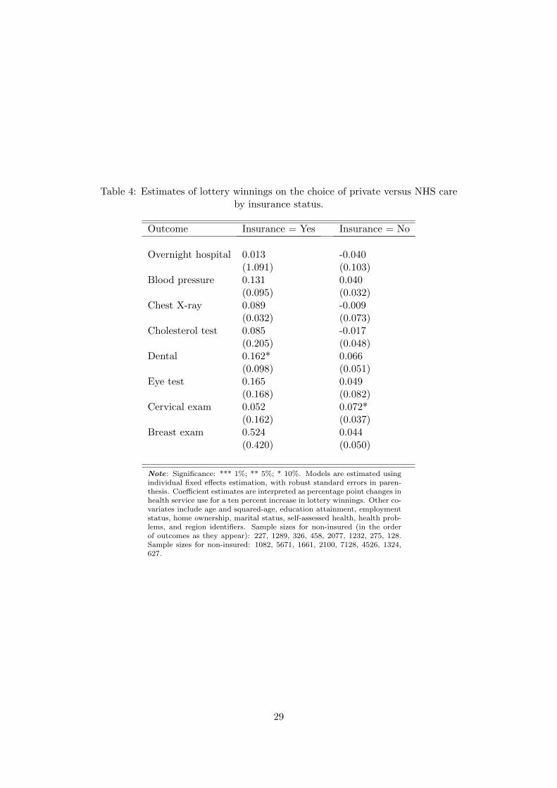
Table 4: Estimates of lottery winnings on the choice of private versus NHS careby insurance status.

Outcome Insurance = Yes Insurance = No

Overnight hospital 0.013 -0.040(1.091) (0.103)

Blood pressure 0.131 0.040(0.095) (0.032)

Chest X-ray 0.089 -0.009(0.032) (0.073)

Cholesterol test 0.085 -0.017(0.205) (0.048)

Dental 0.162* 0.066(0.098) (0.051)

Eye test 0.165 0.049(0.168) (0.082)

Cervical exam 0.052 0.072*(0.162) (0.037)

Breast exam 0.524 0.044(0.420) (0.050)

Note: Significance: *** 1%; ** 5%; * 10%. Models are estimated usingindividual fixed effects estimation, with robust standard errors in paren-thesis. Coefficient estimates are interpreted as percentage point changes inhealth service use for a ten percent increase in lottery winnings. Other co-variates include age and squared-age, education attainment, employmentstatus, home ownership, marital status, self-assessed health, health prob-lems, and region identifiers. Sample sizes for non-insured (in the orderof outcomes as they appear): 227, 1289, 326, 458, 2077, 1232, 275, 128.Sample sizes for non-insured: 1082, 5671, 1661, 2100, 7128, 4526, 1324,627.

29

Table 5: Private medical insurance (PMI) status and lottery wins by insurance types

All types Direct payment &deduct from wages

(1) (2)

(A) Wins > £500 0.022 0.012(0.013) (0.008)

(B) Lottery wins categories:(Reference: £1-£100)

£100 − £250 -0.010 -0.005(0.010) (0.007)

£250 − £500 -0.013 -0.007(0.013) (0.010)

> £500 0.017 0.010(0.014) (0.010)

Observations (N) 10,710 10,419

Note: Significance: *** 1%; ** 5%; * 10%. Results in columns (1) and (2) areestimated using individual fixed effects estimation. Private medical insurancetypes refer to how medical insurance is paid for. Covariates include age andsquared-age, gender, education attainment, employment status, home owner-ship, marital status, self-assessed health, health problems, and region identifiers.

30

Tab

le6:

Lot

tery

win

san

dle

ngt

hof

tim

ein

div

idu

als

mai

nta

inp

riva

tem

edic

alin

sura

nce

cover

age

All

Insu

ran

ceT

yp

esD

irec

tp

aym

ent

&d

edu

ctfr

omw

ages

(N=

570)

(N=

279)

Vari

able

s(1

)(2

)(3

)(4

)(5

)(6

)(7

)(8

)

(A)

Win

s>

£500

-0.8

46**

-0.7

85**

-0.7

55**

-0.5

07-0

.935

*-0

.805

*-0

.667

-0.5

61(0

.353

)(0

.376

)(0

.376

)(0

.389

)(0

.486

)(0

.530

)(0

.551

)(0

.596

)

(B)

Lott

ery

win

sca

tego

ries

:(R

efer

ence

:£

1-£

100)

£10

0−

£250

-0.1

80-0

.203

-0.2

40-0

.136

0.09

60.

202

0.14

10.

154

(0.2

49)

(0.2

56)

(0.2

57)

(0.2

76)

(0.3

95)

(0.4

28)

(0.4

38)

(0.4

62)

£25

0−

£50

0-0

.479

-0.3

75-0

.425

-0.5

010.

335

0.44

60.

309

-0.0

41(0

.339

)(0

.379

)(0

.380

)(0

.412

)(0

.428

)(0

.462

)(0

.453

)(0

.600

)>

£500

-0.8

95**

-0.8

32**

-0.8

06**

-0.5

43-0

.902

*-0

.750

-0.6

35-0

.548

(0.3

57)

(0.3

80)

(0.3

79)

(0.3

92)

(0.4

92)

(0.5

36)

(0.5

54)

(0.5

95)

Tim

ele

ftin

sam

ple

Yes

Yes

Yes

Yes

Yes

Yes

Yes

Yes

Dem

ogra

phic

No

Yes

Yes

Yes

No

Yes

Yes

Yes

Inco

me,

wea

lth

No

No

Yes

Yes

No

No

Yes

Yes

Hea

lth,

geog

raphy

No

No

No

Yes

No

No

No

Yes

Note

:S

ign

ifica

nce

:***

1%

;**

5%

;*

10%

.S

tan

dard

erro

rsare

clu

ster

edat

the

level

of

the

ind

ivid

ual

hen

cep

are

nth

esis

refl

ect

rob

ust

stan

dard

erro

rs.

Th

eou

tcom

evari

ab

leis

the

nu

mb

erof

yea

rsin

div

idu

als

main

tain

pri

vate

med

ical

insu

ran

ceco

ver

age

aft

erta

kin

gu

pm

edic

al

insu

rance

.Tim

eleft

insample

:th

eto

tal

nu

mb

erof

waves

that

ind

ivid

uals

rem

ain

inth

esu

rvey

inth

eyea

rth

eyta

ke

up

med

ical

insu

ran

ce;Dem

ographic

:age

an

dsq

uare

d-a

ge,

gen

der

,m

ari

tal

statu

s,ed

uca

tion

att

ain

men

t,em

plo

ym

ent

statu

s;In

come,

wealth

:h

ou

seh

old

inco

me,

hom

eow

ner

ship

;Health,geography

:se

lf-a

sses

sed

hea

lth

,h

ealt

hp

rob

lem

s,an

dre

gio

nid

enti

fier

s.

31

Tab

le7:

Imp

lied

inco

me

elas

tici

ties

ofh

ealt

hca

rew

ith

resp

ect

tolo

tter

yw

innin

gsan

dh

ouse

hol

din

com

e

Pu

bli

cvs.

No

Car

eP

riva

tevs.

No

Car

eE

last

icit

yE

last

icit

yE

last

icit

yE

last

icit

yof

win

nin

gsof

inco

me

ofw

inn

ings

ofin

com

e(1

)(2

)(3

)(4

)

Ove

rnig

ht

hos

pit

al-0

.012

-0.0

36*

0.22

0*0.

106

Blo

od

pre

ssu

re-0

.009

0.01

7*0.

050

0.10

4***

Ch

est

X-r

ay-0

.004

0.01

80.

260*

*-0

.001

Ch

oles

tero

lte

st-0

.007

0.01

20.

179*

0.15

0***

Den

tal

-0.0

04-0

.011

**-0

.002

0.02

7***

Eye

-tes

t0.

014

-0.0

090.

012

0.05

6***

Cer

vic

al

exam

-0.0

160.

013

0.82

1*0.

511*

**B

reast

exam

0.02

10.

043*

0.12

20.

146

Note

:S

ign

ifica

nce

:***

1%

;**

5%

;*

10%

.M

od

els

are

esti

mate

du

sin

gin

div

idu

al

fixed

effec

tses

tim

ati

on

.S

tati

stic

al

sign

ifica

nt

refe

rsto

the

regre

ssio

nco

effici

ent

esti

mate

s.E

stim

ate

sof

inco

me

elast

icit

ies

are

calc

ula

ted

as

per

centa

ge

chan

ge

inth

ep

rop

ort

ion

of

ind

ivid

uals

ob

tain

ing

pu

blic

or

pri

vate

care

ver

sus

no-c

are

giv

ena

on

e-p

erce

nt

incr

ease

inlo

tter

yw

inn

ings

or

hou

seh

old

inco

me.

32

A Appendix

33

Table A.1: Descriptive statistics of winners and non-winners samples

Winners Non-winners Diff.(N=14,205) (N=134,176)

Whether used health careHospitalisation 9.3% 10.5% ***Blood pressure 49.2% 47.6% ***Chest X-ray 14.0% 13.3% **Cholesterol 18.1% 17.5% *Dental 64.0% 63.5% ***Eye test 40.8% 40.2%Cervical 26.1% 22.8% ***Breast 12.4% 10.9% ***Chose private versus NHS care:Hospitalisation 8.3% 6.1% ***Blood pressure 6.7% 4.7% ***Chest X-ray 6.9% 5.8% **Cholesterol 7.6% 6.3% **Dental 29.4% 26.5% ***Eye test 37.3% 31.0% ***Cervical 15.0% 15.0%Breast 3.7% 3.7%Characteristics:Age (years) 45.3 45.7 **Female 43.2% 55.8% ***Log (real household income) 9.13 9.02 ***Private health insurance 19.7% 14.8% ***Self-assessed health:Excellent 22.6% 23.4% ***Good 48.1% 45.6% ***Fair 20.5% 21.1%Poor 6.7% 7.8% ***Very poor 2.1% 2.2%

Health problems:Arms, Legs etc 29.4% 27.8% ***Sight 5.0% 5.2%Hearing 9.2% 8.3% ***Skin conditions 14.1% 11.7% ***Chest 14.2% 13.5% **Heart/Blood pressure 18.2% 17.1% ***Stomach 8.6% 8.1% *Diabetes 3.8% 3.8%Anxiety, depression 6.9% 8.7% ***Alcohol, drugs 0.5% 0.6%Epilepsy 0.6% 0.9% ***Migraine 8.4% 8.1%Other 5.0% 4.4% ***

Note: Test of difference in group means. Significance: *** 1%; ** 5%; * 10%. Othercovariates not shown include education attainment, employment status, home owner-ship, marital status, and region identifiers.

34

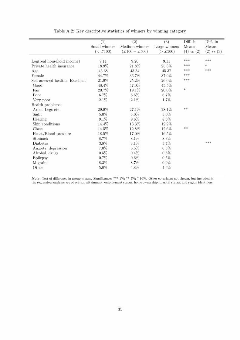
Table A.2: Key descriptive statistics of winners by winning category

(1) (2) (3) Diff. in Diff. inSmall winners Medium winners Large winners Means Means

(< £100) (£100 − £500) (> £500) (1) vs (2) (2) vs (3)

Log(real household income) 9.11 9.20 9.11 *** ***Private health insurance 18.9% 21.8% 25.3% *** *Age 45.68 43.34 45.37 *** ***Female 44.7% 36.7% 37.9% ***Self assessed health: Excellent 21.9% 25.2% 26.0% ***Good 48.4% 47.0% 45.5%Fair 20.7% 19.1% 20.0% *Poor 6.7% 6.6% 6.7%Very poor 2.1% 2.1% 1.7%

Health problems:Arms, Legs etc 29.9% 27.1% 28.1% **Sight 5.0% 5.0% 5.0%Hearing 9.1% 9.6% 8.6%Skin conditions 14.4% 13.3% 12.2%Chest 14.5% 12.8% 12.6% **Heart/Blood pressure 18.5% 17.0% 16.5%Stomach 8.7% 8.1% 8.3%Diabetes 3.8% 3.1% 5.4% ***Anxiety, depression 7.0% 6.5% 6.3%Alcohol, drugs 0.5% 0.4% 0.8%Epilepsy 0.7% 0.6% 0.5%Migraine 8.3% 8.7% 0.9%Other 5.0% 4.8% 4.6%

Note: Test of difference in group means. Significance: *** 1%; ** 5%; * 10%. Other covariates not shown, but included inthe regression analyses are education attainment, employment status, home ownership, marital status, and region identifiers.

35

Tab

leA

.3:

Est

imat

esof

lagg

edlo

tter

yw

inn

ings

onco

nte

mp

oran

eou

slo

tter

yw

ins

Wh

eth

erw

inlo

tter

y(t

)L

oglo

tter

yw

inn

ings

(t)

(1)

(2)

(3)

(4)

(5)

(6)

Wh

eth

erw

inlo

tter

y(t−

1)0.

327*

**-0

.038

***

(0.0

06)

(0.0

03)

Lag

ged

(t−

1)lo

gw

inn

ings

0.09

3***

-0.0

08**

*0.

530*

*-0

.056

***

(0.0

01)

(0.0

01)

(0.0

19)

(0.0

20)

Fix

edeff

ects

No

Yes

No

Yes

No

Yes

Note

:S

ign

ifica

nce

:***

1%

;**

5%

;*

10%

.M

od

els

are

esti

mate

dusi

ng

lin

ear

OL

Sw

ith

rob

ust

stan

dard

erro

rs,

or

ind

ivid

ual

fixed

effec

tses

tim

ati

on

.S

am

ple

sin

colu

mn

s(1

)to

(4)

com

pri

seof

both

win

ner

san

dn

on

-win

ner

s.In

colu

mn

(3)

an

d(4

),la

gged

win

nin

gs

for

non

-win

ner

sare

cod

edas

zero

.S

am

ple

sin

colu

mn

s(5

)an

d(6

)co

mp

rise

on

lyof

win

ner

s.O

ther

covari

ate

sin

clu

de

age

an

dsq

uare

d-a

ge,

edu

cati

on

att

ain

men

t,em

plo

ym

ent

statu

s,h

om

eow

ner

ship

,m

ari

tal

statu

s,se

lf-a

sses

sed

hea

lth

,h

ealt

hp

rob

lem

s,an

dre

gio

nid

enti

fier

s.

36

Table A.4: Coefficient estimates of log lottery winnings at t+1 on winners’ characteristics at t

(1) (2)Fixed Effects OLS

Age 0.027 0.0031(0.024) (0.012)

Age-squared -0.00025 -0.00015(0.00025) (0.00013)

Female -0.213***(0.062)

Education (Ref: Primary)Education: Not defined 0.116 -0.538**

(0.563) (0.243)Secondary 0.265 -0.610***

(1.447) (0.177)Low-secondary, vocation -0.201 -0.161*

(0.454) (0.094)High-secondary, mid-vocation -0.449 -0.248**

(0.476) (0.113)High vocation 0.841 -0.269***

(0.617) (0.103)First degree -0.062 -0.520***

(0.574) (0.132)High degree -0.157 -0.326*

(0.694) (0.184)Log income net winnings 0.084 0.185***

(0.058) (0.046)Employment status (Ref: Paid Employment)Self employed -0.201 0.461***

(0.123) (0.147)Unemployed 0.294* 0.192

(0.167) (0.170)Retired -0.180 0.173

(0.135) (0.116)Family care 0.119 0.150

(0.311) (0.344)Fulltime student 0.204 0.080

(0.147) (0.119)Long term sick/disabled -0.164 -0.295*

(0.221) (0.160)Maternity leave 0.213 0.214

(0.223) (0.167)Government training -0.488 -1.277***

(0.869) (0.338)Other -0.229 0.0513

(0.342) (0.347)Owns home 0.066 -0.068

(0.119) (0.085)Married or defacto -0.098 -0.118

(0.111) (0.075)Self-assessed health (Ref: Excellent)Very Good -0.011 0.00175

(0.060) (0.061)Good -0.015 0.0049

(0.081) (0.082)Continued on next page

37

Table A.4 – continued from previous page(1) (2)Fixed Effects OLS

Fair 0.150 0.028(0.121) (0.124)

Poor 0.035 -0.164(0.186) (0.186)

Health Problems:Arms, Legs etc 0.053 0.026

(0.064) (0.066)Sight -0.098 -0.094

(0.111) (0.106)Hearing -0.091 0.074

(0.110) (0.090)Skin conditions -0.040 -0.034

(0.087) (0.081)Chest 0.0400 0.025

(0.101) (0.078)Heart/Blood pressure -0.0065 -0.013

(0.084) (0.073)Stomach -0.033 0.021

(0.095) (0.097)Diabetes 0.452* 0.160

(0.243) (0.155)Anxiety, depression -0.222* -0.168

(0.116) (0.104)Alcohol, drugs -0.165 0.364

(0.343) (0.463)Epilepsy 0.734 -0.196

(0.630) (0.224)Migraine -0.058 0.0030

(0.100) (0.090)Other 0.285*** 0.138

(0.100) (0.105)Constant 2.303** 2.909***

(0.905) (0.558)

N 5,095 5,095R-squared 0.026 0.049

*** p < 0.01, ** p < 0.05, * p < 0.1. Models are estimated using individual fixed effects and

ordinary least squares estimation. 19 indicator variables reflecting geographical location are

included in the estimation but not presented in the tables for brevity.

38

Tab

leA

.5:

Fix

edeff

ects

esti

mat

esof

hea

lth

serv

ice

use

att

onlo

glo

tter

yw

inn

ings

int+

1

(1)

(2)

(3)

(4)

(5)

(6)

(7)

(8)

Ove

rnig

ht

hos

pit

al0.0

67

(0.0

51)

Blo

od

pre

ssu

re0.

044

(0.0

33)

Ch

est

X-r

ay0.

069

(0.0

43)

Ch

oles

tero

lte

st-0

.033

(0.0

42)

Den

tal

-0.0

74*

(0.0

41)

Eye

test

0.03

4(0

.031

)C

ervic

al

exam

0.03

7(0

.053

)B

reast

exam

0.12

6*(0

.068

)C

on

stan

t3.6

00*

**

3.58

4***

3.59

6***

3.61

2***

3.65

4***

3.59

2***

3.47

0***

3.46

3***

(0.0

11)

(0.0

19)

(0.0

11)

(0.0

13)

(0.0

29)

(0.0

16)

(0.0

20)

(0.0

17)

N11,

718

11,7

1811

,718

11,7

1811

,718

11,7

185,

117

5,11

7

Note

:S

ign

ifica

nce

:***

1%

;**

5%

;*

10%

.R

egre

ssio

nes

tim

ate

sof

wh

eth

erin

div

idu

als

use

dh

ealt

hse

rvic

ein

tim

et

on

log

lott

ery

win

nin

gs

inti

met+

1,

wit

hou

tad

dit

ion

al

covari

ate

s.M

od

els

are

esti

mate

du

sin

gin

div

idu

al

fixed

effec

tses

tim

ati

on

.

39

Tab

leA

.6:

Fix

edeff

ects

esti

mat

esof

the

choi

ceof

pri

vate

vers

us

NH

Sca

reat

ton

log

lott

ery

win

nin

gsin

t+1

(1)

(2)

(3)

(4)

(5)

(6)

(7)

(8)

Ove

rnig

ht

hos

pit

al-0

.152

(0.4

54)

Blo

od

pre

ssu

re-0

.071

(0.1

12)

Ch

est

X-r

ay0.

195

(0.3

63)

Ch

oles

tero

lte

st-0

.159

(0.1

83)

Den

tal

0.05

3(0

.052

)E

yete

st-0

.071

(0.0

63)

Cer

vic

al

exam

-0.2

97(0

.581

)B

reast

exam

-0.5

40(0

.810

)C

on

stan

t3.6

51*

**

3.60

0***

0.19

5***

3.64

5***

3.58

6***

3.62

6***

3.54

0***

3.64

7***

(0.0

49)

(0.0

15)

(0.3

63)

(0.0

25)

(0.0

19)

(0.0

27)

(0.0

33)

(0.0

53)

N1,0

435,

740

1,58

72,

162

7,62

84,

751

1,28

867

6

Note

:S

ign

ifica

nce

:***

1%

;**

5%

;*

10%

.R

egre

ssio

nes

tim

ate

sof

wh

eth

erin

div

idu

als

chose

pri

vate

(non

-NH

S)

care

ver

sus

NH

Sca

rein

tim

et

on

log

lott

ery

win

nin

gs

inti

met+

1,

wit

hou

tad

dit

ion

al

covari

ate

s.M

od

els

are

esti

mate

du

sin

gin

div

idu

al

fixed

effec

tses

tim

ati

on

.

40

Table A.7: Private medical insurance (PMI) status and lottery wins by insurance types:Ever-winners sample

All types Direct payment &deduct from wages

(1) (2)

(A) Any wins 0.003 0.003(0.003) (0.002)

(B) Wins > £500 0.019* 0.005(0.010) (0.008)

(C) Lottery wins categories:No wins (Ref)< £100 0.002 0.003

(0.003) (0.003)£100 − £250 0.004 0.003

(0.008) (0.006)£250 − £500 -0.003 -0.002

(0.011) (0.009)> £500 0.019* 0.005

(0.010) (0.009)

Observations (N) 52,132 46,489

Note: Significance: *** 1%; ** 5%; * 10%. Results in columns (1) and (2)are estimated using individual fixed effects estimation. Private medical insur-ance types refer to how medical insurance is paid for. The sample comprisesof individuals that won the lottery at least once in the panel, lottery players,and consist of both winners and non-winners in a given year. Covariates in-clude age and squared-age, gender, education attainment, employment status,home ownership, marital status, self-assessed health, health problems, and re-gion identifiers.

41

Tab

leA

.8:

Lott

ery

win

san

dle

ngt

hof

tim

ein

div

idu

als

mai

nta

inp

riva

tem

edic

alin

sura

nce

cover

age:

Eve

r-w

inn

ers

sam

ple

All

Insu

ran

ceT

yp

esD

irec

tp

aym

ent

&d

edu

ctfr

omw

ages

(N=

958)

(N=

718)

Vari

able

s(1

)(2

)(3

)(4

)(5

)(6

)(7

)(8

)

(A)

Win

s>

£500

-0.7

71**

-0.7

66**

-0.7

15**

-0.6

33-0

.869

*-0

.809

*-0

.678

-0.6

31(0

.337

)(0

.359

)(0

.358

)(0

.359

)(0

.458

)(0

.462

)(0

.486

)(0

.502

)

(B)

Lott

ery

win

sca

tego

ries

:N

ow

ins

(Ref

)<

£100

0.15

90.

182

0.20

1*0.

215*

0.02

00.

0325

0.06

550.

111

(0.1

19)

(0.1

18)

(0.1

18)

(0.1

19)

(0.1

46)

(0.1

50)

(0.1

49)

(0.1

52)

£10

0−

£250

-0.0

360.

009

-0.0

090.

031

0.11

40.

159

0.14

30.

248

(0.2

29)

(0.2

31)

(0.2

29)

(0.2

31)

(0.3

76)

(0.3

87)

(0.3

89)

(0.3

81)

£25

0−

£50

0-0

.328

-0.2

15-0

.279

-0.3

290.

350

0.40

00.

282

0.15

0(0

.320

)(0

.329

)(0

.334

)(0

.343

)(0

.411

)(0

.410

)(0

.408

)(0

.438

)>

£500

-0.7

39-0

.725

**-0

.669

*-0

.585

-0.8

54*

-0.7

88*

-0.6

53-0

.591

(0.3

37)

(0.3

59)

(0.3

58)

(0.3

59)

(0.4

59)

(0.4

64)

(0.4

88)

(0.5

04)

Tim

ele

ftin

sam

ple

Yes

Yes

Yes

Yes

Yes

Yes

Yes

Yes

Dem

ogra

phic

No

Yes

Yes

Yes

No

Yes

Yes

Yes

Inco

me,

wea

lth

No

No

Yes

Yes

No

No

Yes

Yes

Hea

lth,

geog

raphy

No

No

No

Yes

No

No

No

Yes

Note

:S

ign

ifica

nce

:***

1%

;**

5%

;*

10%

.S

tan

dard

erro

rsare

clu

ster

edat

the

level

of

the

ind

ivid

ual

hen

cep

are

nth

esis

refl

ect

rob

ust

stan

dard

erro

rs.

Th

esa

mp

leco

mp

rise

sof

ind

ivid

uals

that

won

the

lott

ery

at

least

on

cein

the

pan

el,

lott

ery

pla

yer

s,an

dco

nsi

stof

both

win

ner

san

dn

on

-win

ner

sin

agiv

enyea

r.T

he

ou

tcom

evari

ab

leis

the

nu

mb

erof

yea

rsin

div

idu

als

main

tain

pri

vate

med

ical

insu

ran

ceco

ver

age

aft

erta

kin

gu

pm

edic

al

insu

rance

.Tim

eleft

insample

:th

eto

tal

nu

mb

erof

waves

that

ind

ivid

uals

rem

ain

inth

esu

rvey

inth

eyea

rth

eyta

ke

up

med

ical

insu

ran

ce;Dem

ographic

:age

an

dsq

uare

d-a

ge,

gen

der

,m

ari

tal

statu

s,ed

uca

tion

att

ain

men

t,em

plo

ym

ent

statu

s;In

come,

wealth

:h

ou

seh

old

inco

me,

hom

eow

ner

ship

;Health,geography

:se

lf-a

sses

sed

hea

lth

,h

ealt

hp

rob

lem

s,an

dre

gio

nid

enti

fier

s.

42

Table A.9: Implied income elasticities of health carewith respect to inheritance income

Public vs. Private vs.Dependent variable No Care No Care

Overnight hospital 0.039 0.138

Blood pressure 0.013 0.082

Chest X-ray -0.006 0.769

Cholesterol test 0.010 0.033

Dental 0.012 0.058**

Eye test 0.008 0.143***

Cervical exam 0.044* 0.224

Breast exam 0.033 0.171

Note: −a Significance: *** 1%; ** 5%; * 10%. Statistical significancerefers to the regression coefficient estimates, which are estimated usingOLS. Estimates of income elasticities are calculated as percentage changein the proportion of individuals obtaining public or private care versusno-care given a one-percent increase in bequest income.

43