WP/08/24

Do Technology Shocks Lead to Productivity Slowdowns? Evidence from

Patent Data

Lone E. Christiansen

© 2008 International Monetary Fund WP/08/24 IMF Working Paper Research Department

Do Technology Shocks Lead to Productivity Slowdowns? Evidence from Patent Data

Prepared by Lone E. Christiansen1

Authorized for distribution by Alessandro Prati

January 2008

Abstract

This Working Paper should not be reported as representing the views of the IMF. The views expressed in this Working Paper are those of the author(s) and do not necessarily represent those of the IMF or IMF policy. Working Papers describe research in progress by the author(s) and are published to elicit comments and to further debate.

This paper provides empirical evidence on the response of labor productivity to the arrival of new inventions. The benchmark measure of technological progress is given by data on patent applications in the U.S. over the period 1889–2002. The analysis shows that labor productivity may temporarily fall below trend after technological progress. However, the effects on productivity differ between the pre- and post-World War II periods. The pre-war period shows evidence of a productivity slowdown as a result of the arrival of new technology, whereas the post-World War II period does not. Positive effects of technology shocks tend to show up sooner in the productivity data in the later period. JEL Classification Numbers: 030, 040 Keywords: Productivity, patents, technology Author’s E-Mail Address: Lchristiansen@imf.org

1 I thank Bryan Goudie, Bronwyn Hall, Nir Jaimovich, Garey Ramey, Valerie Ramey, and Mark Schankerman for helpful comments and suggestions. I thank W. Michael Cox at the Federal Reserve Bank of Dallas for kindly providing data on diffusion of products and Nestor Terleckyj for kindly providing historical R&D data and directing me to important, relevant literature

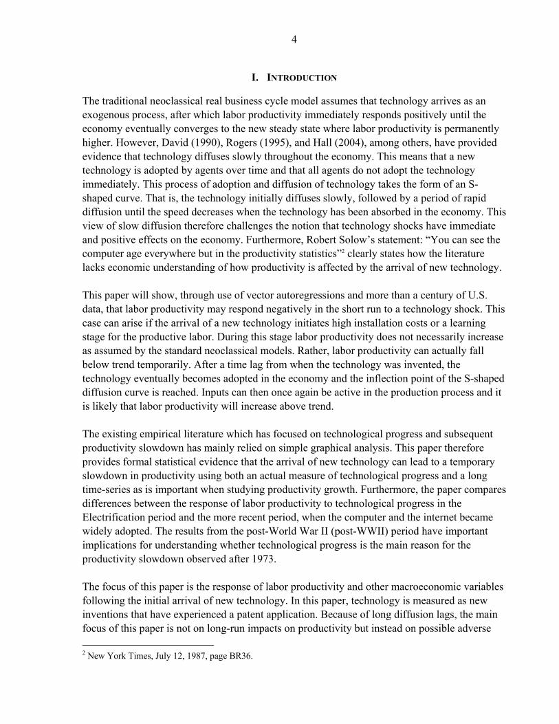
2 Contents Page

I. Introduction ............................................................................................................................4

II. Existing Literature.................................................................................................................5

III. Data ......................................................................................................................................7

IV. Methodology......................................................................................................................12

V. Empirical Evidence .............................................................................................................13 A. Benchmark Specification ........................................................................................13 B. Robustness of the Results........................................................................................17

VI. Pre- and Post-WWII ..........................................................................................................21 A. VAR Estimation on Two Sample Periods...............................................................22 B. Post-WWII VECM..................................................................................................23 C. Variance Decomposition .........................................................................................24

VII. Theoretical Implications of the Results............................................................................25

VIII. Conclusion ......................................................................................................................26 Tables 1. Augmented Dickey Fuller Unit Root Tests .........................................................................27 2. Granger Causality Tests.......................................................................................................27 3. Great Inventions...................................................................................................................28 4. Exclusion Tests in a Restricted Model.................................................................................29 5. Coefficient Estimates of the Restricted Model ....................................................................30 6. Parameter Estimates for the Restricted Model.....................................................................31 7. Cointegration in Post-WWII Data .......................................................................................31 8. Variance Decomposition......................................................................................................32 Figures 1. The Flow of Technologies ...................................................................................................34 2. Patents and Productivity ......................................................................................................34 3. Total Patent Applications and Patents Granted ...................................................................34 4. Diffusion of Aggregate Electric Power in Manufacturing...................................................35 5. Spread of Products into American Households ...................................................................35 6. Responses of Patents and Productivity to a Patent Shock, 1889–2002. ..............................36 7. Responses to a Patent Shock................................................................................................38 8. Stock Prices, 1889–2002......................................................................................................40 9. The Stock of Patents ............................................................................................................41 10. Shock to the Stock of Patents, 1889–2002.........................................................................42 11. Responses to a Patent Shock in a Restricted Model, 1889–2002 ......................................42 12. Response of Productivity to an R&D and a Patent Shock, 1935–1997.............................43 13. Two Sample Periods ..........................................................................................................44 14. Responses from a Post-WWII VECM, 1948–2002 ...........................................................46 15. Responses from a Post-WWII VAR, 1948–2002 ..............................................................47

3 Appendix..................................................................................................................................50 References................................................................................................................................51

4

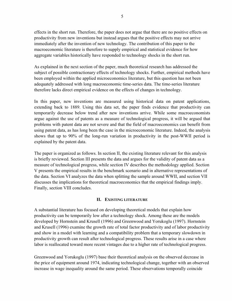
I. INTRODUCTION

The traditional neoclassical real business cycle model assumes that technology arrives as an exogenous process, after which labor productivity immediately responds positively until the economy eventually converges to the new steady state where labor productivity is permanently higher. However, David (1990), Rogers (1995), and Hall (2004), among others, have provided evidence that technology diffuses slowly throughout the economy. This means that a new technology is adopted by agents over time and that all agents do not adopt the technology immediately. This process of adoption and diffusion of technology takes the form of an S-shaped curve. That is, the technology initially diffuses slowly, followed by a period of rapid diffusion until the speed decreases when the technology has been absorbed in the economy. This view of slow diffusion therefore challenges the notion that technology shocks have immediate and positive effects on the economy. Furthermore, Robert Solow’s statement: “You can see the computer age everywhere but in the productivity statistics”2 clearly states how the literature lacks economic understanding of how productivity is affected by the arrival of new technology. This paper will show, through use of vector autoregressions and more than a century of U.S. data, that labor productivity may respond negatively in the short run to a technology shock. This case can arise if the arrival of a new technology initiates high installation costs or a learning stage for the productive labor. During this stage labor productivity does not necessarily increase as assumed by the standard neoclassical models. Rather, labor productivity can actually fall below trend temporarily. After a time lag from when the technology was invented, the technology eventually becomes adopted in the economy and the inflection point of the S-shaped diffusion curve is reached. Inputs can then once again be active in the production process and it is likely that labor productivity will increase above trend. The existing empirical literature which has focused on technological progress and subsequent productivity slowdown has mainly relied on simple graphical analysis. This paper therefore provides formal statistical evidence that the arrival of new technology can lead to a temporary slowdown in productivity using both an actual measure of technological progress and a long time-series as is important when studying productivity growth. Furthermore, the paper compares differences between the response of labor productivity to technological progress in the Electrification period and the more recent period, when the computer and the internet became widely adopted. The results from the post-World War II (post-WWII) period have important implications for understanding whether technological progress is the main reason for the productivity slowdown observed after 1973. The focus of this paper is the response of labor productivity and other macroeconomic variables following the initial arrival of new technology. In this paper, technology is measured as new inventions that have experienced a patent application. Because of long diffusion lags, the main focus of this paper is not on long-run impacts on productivity but instead on possible adverse 2 New York Times, July 12, 1987, page BR36.

5 effects in the short run. Therefore, the paper does not argue that there are no positive effects on productivity from new inventions but instead argues that the positive effects may not arrive immediately after the invention of new technology. The contribution of this paper to the macroeconomic literature is therefore to supply empirical and statistical evidence for how aggregate variables historically have responded to technology shocks in the short run. As explained in the next section of the paper, much theoretical research has addressed the subject of possible contractionary effects of technology shocks. Further, empirical methods have been employed within the applied microeconomics literature, but this question has not been adequately addressed with long macroeconomic time-series data. The time-series literature therefore lacks direct empirical evidence on the effects of changes in technology. In this paper, new inventions are measured using historical data on patent applications, extending back to 1889. Using this data set, the paper finds evidence that productivity can temporarily decrease below trend after new inventions arrive. While some macroeconomists argue against the use of patents as a measure of technological progress, it will be argued that problems with patent data are not severe and that the field of macroeconomics can benefit from using patent data, as has long been the case in the microeconomic literature. Indeed, the analysis shows that up to 90% of the long-run variation in productivity in the post-WWII period is explained by the patent data. The paper is organized as follows. In section II, the existing literature relevant for this analysis is briefly reviewed. Section III presents the data and argues for the validity of patent data as a measure of technological progress, while section IV describes the methodology applied. Section V presents the empirical results in the benchmark scenario and in alternative representations of the data. Section VI analyzes the data when splitting the sample around WWII, and section VII discusses the implications for theoretical macroeconomics that the empirical findings imply. Finally, section VIII concludes.

II. EXISTING LITERATURE

A substantial literature has focused on developing theoretical models that explain how productivity can be temporarily low after a technology shock. Among these are the models developed by Hornstein and Krusell (1996) and Greenwood and Yorukoglu (1997). Hornstein and Krusell (1996) examine the growth rate of total factor productivity and of labor productivity and show in a model with learning and a compatibility problem that a temporary slowdown in productivity growth can result after technological progress. These results arise in a case where labor is reallocated toward more recent vintages due to a higher rate of technological progress. Greenwood and Yorukoglu (1997) base their theoretical analysis on the observed decrease in the price of equipment around 1974, indicating technological change, together with an observed increase in wage inequality around the same period. These observations temporally coincide

6 with the measured slowdown in labor productivity growth. Following these observations, Greenwood and Yorukoglu (1997) develop a model where the firm produces at a variety of plants using capital together with both skilled and unskilled labor as inputs. The model shows that an increase in the growth rate of investment-specific technological change leads to higher income inequality during a learning period since skilled labor is relatively higher priced during this period. Furthermore, labor productivity growth slows down since application of the new technology takes time and because the new technology does not work at full capacity immediately after adoption as a result of the importance of learning. In empirical studies of productivity growth, Gali (1999) and Francis and Ramey (2004) identify technology shocks through a structural vector autoregression (VAR) using long-run restrictions. Gali (1999) assumes that labor productivity is characterized by a unit root which is driven solely by technology shocks. That is, technology shocks have a permanent effect on productivity and any permanent effects originate solely from these shocks. However, if variables other than technology affect long-run productivity, then the assumption used to identify the technology shocks is violated. Short-run effects based on long-run restrictions might therefore be unreliable. Thus, avoiding this restriction seems important when analyzing temporary short-run effects as done in this paper. Further, if productivity is trend stationary with deterministic breaks, then the long-run restrictions are invalid and can result in misleading conclusions. To avoid using identifying long-run restrictions an alternative is to compute technology series based on total factor productivity. Basu, Fernald, and Kimball (2006) construct a measure intended to capture aggregate technology. Their technology series is based on aggregate total factor productivity, controlled for varying utilization of capital and labor, non-constant returns and imperfect competition, and aggregation effects. However, total factor productivity remains a residual that likely includes other factors than technology. An alternative approach is therefore to use a direct measure of technological change which is empirically observed. One of the pioneers in using patent statistics as indicators of inventive output was Jacob Schmookler. He examined relations between inventive and economic activity and explored the relation between successful innovations and capital investment. The study in Schmookler (1972) contains an extensive list of patent statistics. Several studies in the patent literature have concluded that patent counts do have important information relevant for measuring technological progress and knowledge (Lach, 1995), among others). Furthermore, Hall and Trajtenberg (2004) find that highly cited patents are important when identifying periods with diffusion and development of a general purpose technology (GPT)3. This is done by exploiting information on the number of patent citations received and in generality measures based on the NBER patent citations data file which is described in Hall, Jaffe, and Trajtenberg (2001).

3 A General Purpose Technology (GPT) is described in Hall and Trajtenberg (2004) as a new technology that is extremely pervasive and used in many sectors of the economy and is subject to continuous technical advance after it has first been introduced.

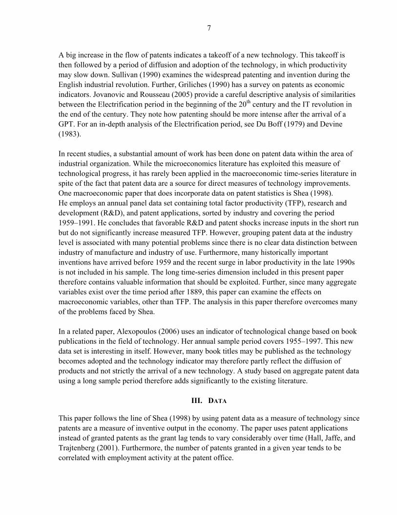
7 A big increase in the flow of patents indicates a takeoff of a new technology. This takeoff is then followed by a period of diffusion and adoption of the technology, in which productivity may slow down. Sullivan (1990) examines the widespread patenting and invention during the English industrial revolution. Further, Griliches (1990) has a survey on patents as economic indicators. Jovanovic and Rousseau (2005) provide a careful descriptive analysis of similarities between the Electrification period in the beginning of the 20th century and the IT revolution in the end of the century. They note how patenting should be more intense after the arrival of a GPT. For an in-depth analysis of the Electrification period, see Du Boff (1979) and Devine (1983). In recent studies, a substantial amount of work has been done on patent data within the area of industrial organization. While the microeconomics literature has exploited this measure of technological progress, it has rarely been applied in the macroeconomic time-series literature in spite of the fact that patent data are a source for direct measures of technology improvements. One macroeconomic paper that does incorporate data on patent statistics is Shea (1998). He employs an annual panel data set containing total factor productivity (TFP), research and development (R&D), and patent applications, sorted by industry and covering the period 1959–1991. He concludes that favorable R&D and patent shocks increase inputs in the short run but do not significantly increase measured TFP. However, grouping patent data at the industry level is associated with many potential problems since there is no clear data distinction between industry of manufacture and industry of use. Furthermore, many historically important inventions have arrived before 1959 and the recent surge in labor productivity in the late 1990s is not included in his sample. The long time-series dimension included in this present paper therefore contains valuable information that should be exploited. Further, since many aggregate variables exist over the time period after 1889, this paper can examine the effects on macroeconomic variables, other than TFP. The analysis in this paper therefore overcomes many of the problems faced by Shea. In a related paper, Alexopoulos (2006) uses an indicator of technological change based on book publications in the field of technology. Her annual sample period covers 1955–1997. This new data set is interesting in itself. However, many book titles may be published as the technology becomes adopted and the technology indicator may therefore partly reflect the diffusion of products and not strictly the arrival of a new technology. A study based on aggregate patent data using a long sample period therefore adds significantly to the existing literature.

III. DATA

This paper follows the line of Shea (1998) by using patent data as a measure of technology since patents are a measure of inventive output in the economy. The paper uses patent applications instead of granted patents as the grant lag tends to vary considerably over time (Hall, Jaffe, and Trajtenberg (2001). Furthermore, the number of patents granted in a given year tends to be correlated with employment activity at the patent office.

8 Since the NBER patent citation database only contains citations made after 1975 this paper focuses on total annual utility patent applications received by the United States Patent and Trademark Office (USPTO) in the period 1889–2002. The paper focuses on utility patents since these are considered as invention patents by the USPTO.4 This also corresponds to Hall, Jaffe, and Trajtenberg (2001) who include utility patents in the patent citations data file. For purposes of identifying the economic response of productivity to technology improvements, using patent data offers an advantage over imposing long-run restrictions, because controversial assumptions about which shocks will affect productivity in the long run are not required. However, as mentioned by Shea (1998) there are drawbacks to using patent data. Namely, changes in patent laws can change the incentive to apply for patents, not all inventions are patented, and the importance of specific inventions varies over time. However, as mentioned in section II, patents do contain important information about technological progress. The number of patents granted is correlated with changes in patenting activity at the USPTO due to variation in budgetary resources over the administrative cycle, leading to budgetary effects in the granting activity. Furthermore, there may be changes at the patent office which lead to changes in the granting rates over time. On the contrary, this paper employs patent applications, which should be less affected by changes in the patenting activity at the USPTO than data on granted patents. As such, it is not necessary to control for variations in patenting activity due to changes at the patent office. However, using patent applications results in the problem that inventions which are not considered sufficiently unique and therefore are not patented are included in the data. For the present analysis, this is not a severe problem since arrival of a new GPT should lead to a surge of patent applications, as explained by Jovanovic and Rousseau (2005). To the extent that interest lies in exploiting the information about changes in economically important technological progress, patent application data do become a good indicator. Another potential problem with patent data is that patenting can be considered a strategic decision, and some firms may choose to keep their inventions secret rather than patent them. However, Trajtenberg (2001) notes that it is widely believed that these limitations are not too severe and argues that they do not affect trends or variation over time. Because this paper uses the time-series variation in the patent data, these limitations are not important. For the present analysis it is important to note that patents measure inventions and not innovations5. It is very likely that there is a lag between the arrival of a new invention and its 4 Other types of patents are plant patents and design patents. Plant patents can be granted to “anyone who has invented or discovered and asexually reproduced any distinct and new variety of plant, including cultivated sports, mutants, hybrids, and newly found seedlings” (USPTO). Design patents refer to a new design of a product. In most years, utility patents account for more than 93% of total patents and the results in the paper are not sensitive to using total patent applications.

5 Innovation indicates first use of a given invention.

9 full use in the macroeconomy, as shown in figure 1. Furthermore, if the economy-wide adoption of new technology is sufficiently slow it is possible for the economy to slow down temporarily after the arrival of a new invention; positive effects may not arise until the technology has been sufficiently adopted. Another argument for using patent data as a measure of technological progress is the importance of news. Ramey (2006) shows how estimates of the effects of government spending shocks change dramatically if the initial anticipation of government spending is not taken into account. For the present paper, where technology shocks are the center of attention, this problem is particularly important, because technology affects the economy through slow diffusion. Considering shocks that have only immediate and positive effect on productivity may potentially exclude very important information about temporary adverse effects of technological progress. Using information from the patent data about the time of invention enables the analysis in this paper to capture the full effects of technology shocks. As the measure of productivity, the paper uses labor productivity, calculated as output per hour; the historical data come from Kendrick (1961). Details of the data, including other variables used and their sources, are described in the appendix. The natural logarithm is taken of all variables. The logarithm of the flow of total utility patent applications is illustrated in panel A of figure 2 and the logarithm of labor productivity and labor productivity growth are illustrated in panel B. The paper uses labor productivity instead of total factor productivity (TFP) in order to avoid some of the problems mentioned in Nordhaus (2005). Namely, the inputs of capital services are not observed directly and therefore must be estimated with specific assumptions when calculating TFP. See Nordhaus (2005) and references therein for a further discussion of this issue. As a robustness check, the calculations in this paper were also done with TFP in place of labor productivity. This did not change the conclusions and these results are therefore not reported. Figure 3 plots total patent applications together with total patents granted by year. The overall movements in these two series are similar, but the variation in the application-grant lag in some periods leads to a shift in the series on granted patents. For example, the surge of applications in the second half of the 1930s does not show up in the grant series until the first half of the 1940s. Similar shifts in the grant series can be seen in the second half of the 1940s and in the 1950s. Further, during the 1970s we observe a decrease in the number of patents granted while patent applications remained constant. In general, budget cuts at the USPTO lead to fluctuations in the grant series that are not present in the applications series. Based on the theoretical findings of Greenwood and Yorukoglu (1997), this paper also examines whether wage inequality changes as a result of technological progress. Data on income and wage inequality are taken from Piketty and Saez (2003). They collected annual data from the Internal Revenue Service back to 1913, which signified the beginning of the modern

10 U. S. income tax. Data on income and wage inequality cover the period 1917–1998 and 1927–1998, respectively. The data include the income and wage shares of total income and wages for the top decile of tax units6. The income shares are calculated by dividing the income for a given fractile by total personal income from the National Income Accounts7. Wage shares are computed using an equivalent methodology, though linear interpolation is used where a few observations are missing. Piketty and Saez mention that the Tax Reform Act of 1986 and World War II are important for the development of the data series. During World War II, for example, there is a sharp drop in wage shares of the top decile, and this paper controls for this by including dummy variables whenever these variables are included in the estimation. Figure 2, panel B illustrates how labor productivity clearly has an upward trend. This may be due to an inherent unit root with drift or to a deterministic trend. Table 1 presents the results of Augmented Dickey Fuller unit root tests for labor productivity and patent applications under different assumptions for the alternative hypothesis. According to these tests, the paper cannot reject a unit root in productivity or patents in levels. Tests were also performed for unit roots in differences. These tests were all rejected and are not reported here. If both time-series are integrated of order one, I(1), it is important to test for cointegration in the data. However, cointegration tests for the full sample (not shown) reject the presence of cointegrating vectors when allowing for a linear trend in the data. It can therefore be concluded that a VAR(p-1) in log differences can be estimated. However, ignoring efficiency considerations, estimation can also be performed as a VAR(p) in levels and results of this estimation are described in section V. An important issue when testing for unit roots is that unit root tests are hard to reject if a coefficient is close to one. It is likely that the patent-productivity system is stationary around a trend. Perron (1989) considered the null hypothesis that a time series has a unit root with possibly nonzero drift against the alternative that the process is trend-stationary. In this specification he showed that one can reject the hypothesis of a unit root for most macroeconomic time-series when the alternative allows for an exogenous break in trend. Following Perron (1989), the exogenous break can in the pre-World War II (pre-WWII) period be estimated as a change in the intercept for the crash in 1929. For the oil price shock in 1973 the break can be estimated as a change in the slope of the time trend. To allow for a Perron-type specification, this paper estimates a number of VARs with different assumptions, including time trends, breaks in trend, and dummy variables whenever necessary. Results of these estimations are reported in section V.

6 A tax unit is defined as “a married couple living together (with dependents), or a single adult (with dependents), as in the current tax law” (Piketty and Saez (2003)).

7 Piketty and Saez (2003) note that this is the standard procedure when computing income inequality measures in historical studies.

11 True exogenous technology shocks should not be predictable by past observations of productivity. In order to test whether the measure of technology shocks used here satisfies this requirement, this paper presents Granger Causality tests with patents and productivity in table 2, panel A. The tests are done both in levels and in differences to avoid any inference problems caused by possible unit roots. It can be seen in the table that patents Granger Cause productivity and that the Granger causality does not run in the opposite direction. This, again, argues for the validity of patent data as a measure of exogenous technological progress. That patent application data despite their noisy component can be used as a measure of the arrival of major inventions can also be seen by examining a few historically known technological advances. Examples from the beginning of the sample period include the arrival of the first hydro-electric facility in 1894, the discovery of X-rays in 1895, the airplane in 1903 and the radio in 1906, all of which are of great importance for development of future inventions. And all of these inventions were followed by an increase in patent applications. The second half of the 1930s also showed an increase in patent applications. This observation is consistent with Mensch (1975) who found that the years around 1935 were characterized by a large number of basic innovations which were important for further technological development. In more recent years, one of the most important new GPTs was the internet, which arrived in 1991 during a surge in patenting. An important issue concerning technological progress is the possible endogeneity of new inventions. As an example, R&D expenditures are important for development of new products. However, if the big changes in the flow of patents over the sample period are thought of as arrival of new GPTs, then these may tend to be less correlated with R&D expenditures. As a robustness check, section V also includes R&D expenditures in the analysis. On the contrary, if we consider adoption of new products in the economy, Comin and Hobijn (2004) showed that real GDP per capita is very important for the rate of adoption of a new technology as is the level of schooling. For many products a network effect is also in place. When examining the diffusion curves for different products we therefore observe the well known S-shape as described earlier. Figure 4 illustrates the S-shaped diffusion curve for aggregate electric power in American manufacturing. Figure 5 is a graph of how different inventions became adopted by American households. Note that there is a significant lag from the start of the diffusion process till it reaches its inflection point. Further, there is a lag between the initial date of invention, which for some products can be seen in table 3, and the start of the diffusion process. This lag tends to be shorter for more recent inventions just as the diffusion evolves at a faster rate. Alm and Cox (1996) address the fact that as the economy evolves, it takes less and less time for new products to become adopted. An example is the internet which was adopted at a rate that exceeded historically observed rates for other GPTs. This faster rate of diffusion in the later period indicates that any observed negative effects after new inventions may be shorter-lived in the second half of the sample than in the first half.

12

IV. METHODOLOGY

The benchmark model originates from a bivariate VAR with patents and labor productivity. Estimates are computed through a recursively identified structural VAR with patents as the first variable and productivity as the second. This corresponds to the assumption that patents are only affected by productivity with a lag, whereas productivity can respond to contemporaneous changes in patents. Using this ordering allows for productivity adjustments because of changes in expectations of future profitability after news of new inventions.8 The unrestricted reduced form VAR can be written as

ttptpttt xyyycy ε+Γ+Φ++Φ+Φ+= −−− ...2211 . ( 1 )

Here, yt is an n × 1 vector of the n endogenous variables in the VAR. As such, yt contains patents and productivity in the benchmark specification. When the paper allows for other variables to enter the system these variables will appear as the third variable in yt. xt is a vector of exogenous variables. εt is a vector of error terms, while c is a vector of constants. Φi, where i = 1,…p, are matrices of coefficients on lagged observations of yt, and Γ is a matrix of coefficients for the exogenous variables. Let Ω denote the variance-covariance matrix of the error terms such that ( ) '' PPE tt ==Ω εε , where P is a lower triangular matrix computed by Cholesky factorization. Following Hamilton (1994), let F denote the matrix of coefficient estimates such that

⎟⎟⎟⎟⎟⎟

⎠

⎞

⎜⎜⎜⎜⎜⎜

⎝

⎛ ΦΦΦΦ

=

−

nnnn

nnnn

nnnn

nnnn

pp

I

II

F

0...0000...0000...000...0

... 121

, ( 2 )

where In is an n × n identity matrix and 0n is an n × n matrix of zeros. The orthogonalized impulse response functions from a unit shock to yj s periods into the future can then be written as

( )jj

js

jt

pttjttst

PPF

yyyyyyE 1,...,,,...,ˆ

1111 ⋅=

∂∂ −−+ , for s = 1, …, h, ( 3 )

where sF11 is the first n rows and n columns of Fs, Pj is the jth column of P, and Pjj is the (j,j) element of P. Thus, whenever the paper analyzes responses to a shock in a variable, the paper

8 The paper also tried different ordering of the variables. This did not change the overall conclusions.

13 considers a shock to the corresponding orthogonalized error term.9 With this specification, the imputed impulse response functions will depict the change in the forecast that occurred as a result of shocking one of the endogenous variables in the system. The impulse response functions will therefore illustrate changes in a variable, relative to the trend the given variable would otherwise have followed had the given variable not experienced a shock. As such, when the paper talks about negative or positive responses of variables to a technology shock, this should be interpreted as revisions in forecasts such that the given variable is forecasted to be below or above the initially forecasted level. That is, a negative response does not necessarily imply an actual fall in the level of the variable but indicates a slowdown relative to the initially forecasted path.

V. EMPIRICAL EVIDENCE

A. Benchmark Specification

In section III, the paper found that unit roots cannot be rejected in the productivity and patent data. If it is assumed that these two variables have a unit root, this would argue for estimating the VAR in log differences in order to obtain stationarity. However, since both estimations in log differences and in log levels are consistent, both estimations are performed on the full sample.10 The two specifications show impulse response functions that are very similar, and the paper therefore only reports the results as estimated in log levels. As mentioned above, Perron (1989) found that many macroeconomic time-series are stationary around a trend if we allow for a break in trend. The bivariate VAR is therefore also estimated with time trends. Using this specification, the paper follows Perron (1989) and allows for a change in the intercept in 1930 in the beginning of the great depression and for a break in trend in 1973, following the oil shock.11 To determine the optimal lag-length in the VAR the Akaike Information Criterion (AIC) is estimated. The AIC suggests using p = 5 lags when estimating the VAR in levels. However, if the true lag-length is finite, the AIC estimate will not be consistent. See Bhansali (1997) for an analysis of this. To reduce the small sample bias, the paper therefore chooses p = 4 lags when estimating the VAR in levels12 and p = 3 lags when estimating the VAR in differences. On figure 2, panel A, patent data appear to have a break in trend in 1985. This could potentially be due partly to a change in the patent law in 1985 that may have affected the incentive to apply for a patent. The analysis can control for this by including a break in trend in 1985. The impulse

9 The impulse response functions are computed based on one standard deviation shocks, corresponding to not dividing by Pjj.

10 Estimating in differences in the presence of unit roots is more efficient than estimating in levels. However, the levels estimation is consistent and often preferred to the difference estimation in order to avoid possible misspecification.

11 See Ramey and Shapiro (1998) for another example of a Perron type time trend.

12 The paper also tried using p = 5 lags. This did not change the overall conclusions.

14 response functions that result from a bivariate VAR with patents and productivity after a one standard deviation shock to patents are illustrated in figure 6 under different specifications. Panel A of figure 6 shows the responses using a VAR in levels without any time trends or dummies in the regressions. Panels B, C, and D of figure 6 include time trends with breaks in trend. The responses are plotted together with 2 standard deviation error bands. In figure 6, patents respond positively to a patent shock and in specifications where a time trend is included, the trend-stationarity leads to no permanent effects. Productivity temporarily decreases relative to the initially forecasted level after a positive patent shock under all specifications, and productivity slowly converges back to the initially forecasted level. This result supports the hypothesis of Hornstein and Krusell (1996) who examined if technology improvements can cause productivity slowdowns. If the response of productivity is examined in the Perron-type specification, including dummies for WWII and the Great Depression, at a horizon longer than 10 years, the response function (not shown) increases insignificantly above the originally forecasted level, indicating that productivity eventually will be positively affected by a technology shock. Furthermore, many researchers prefer to analyze detrended time series data so this paper also estimated the VAR with the full sample of HP-filtered13 data. The resulting impulse response functions are depicted in figure 6, panel E. Using HP-filtered data did not change the conclusions of a temporary productivity slowdown. However, the positive effects in this case show up sooner than in the case of a Perron-type specification.

For the following analysis a benchmark model must be selected. The paper chooses to follow Perron (1989) and include a time trend, allowing for breaks. The benchmark specification can therefore be written as

tttt

ttptpttt

timeWWIIGDDtimeyyycy

ελδγ

βα

+⋅+⋅+⋅+

⋅+⋅+Φ++Φ+Φ+= −−−

7329...2211

( 4 )

where the notation is as in section IV. Additionally, timet is a time trend starting in 1889, and D29t is a dummy variable such that D29t = 1 for t > 1929 and 0 otherwise. GDt is a dummy variable that takes the value of 1 in 1931–33 in order to account for the Great Depression. WWIIt is a dummy variable such that WWIIt = 1 for t = 1941-45, and time73t is a time trend starting in 1973. A break in trend in 1985 is left out because it has little effect on the standard errors of the regressions and on R2.14 Furthermore, Kortum and Lerner (1998) examined the surge in patenting after 1985. They examined if this recent increase is a result of changes in patent laws in the U.S., a widening set of technological opportunities, or a change in the management of R&D facilities. They concluded that the recent surge in U.S. domestic patenting

13 HP filter denotes the Hodrick-Prescott filter. An HP parameter, λ, of 400 was used.

14 Including a break in trend in 1985 does not change the overall conclusions. In most cases it only further decreases the response of productivity to a shock to patents.

15 is correlated with an increase in patenting abroad by U.S. inventors and is not specific to U.S. patent law changes. This suggests that a surge in discovery and innovation started around 1985 and argues for not including a break in trend in 1985. Instead, the change is left as variation in the flow of patents, resulting from the arrival of new technology. Piketty and Saez (2003) mention that the Tax Reform Act of 1986 may temporarily have affected income inequality measures as 1987 and 1988 experienced a relatively large gain in inequality with no permanent level effects. The paper therefore includes a dummy for the two years following the Tax Reform Act when income inequality measures are included. To find support for the argument that technological progress can lead to productivity slowdowns, the response of other variables must be examined. A trivariate VAR is estimated with patents and productivity as the first two variables and a variable Dt as the third variable15. Dt will represent variables such as real consumption, gross private investment, output, and an index of stock market prices, among others. Only one of these variables enters at a time according to the measure of interest. The resulting impulse response functions of a shock to patents are shown in Figure 7. Each row in figure 7, panel A, indicates a different VAR with a different Dt. The response functions depicted in figure 7, panel B, are from different trivariate VARs. Labor productivity shows a transitory slowdown after a patent shock, although insignificant at the 5 percent level in the case of output and hours as the third variable. Note that when consumption and hours are included in the analysis, the response of productivity after 6 years is positive, although insignificant at the 5 percent level. This indicates that the new technology does have a positive effect on labor productivity as is expected from theory. However, the time lag until the response is positive is longer than the standard theory would suggest. Consumption increases after a patent shock. This is consistent with the notion that consumers expect an increase in their future stream of income after the arrival of new technology. In order to smooth consumption, consumers increase consumption immediately. Panel A of figure 7 also reports the response of real GDP, which decreases temporarily. Correspondingly, the paper finds a large and significant short-run increase in consumption’s share of income after a patent shock. This reflects the importance of consumption smoothing after news arrives about new technology. Figure 7, panel A, also shows the response of output in the private economy. Here it can be observed that private output does not respond significantly. The response of investment is insignificant and a clear conclusion cannot be made in this case. There is some indication that investment may be increasing in the short run, which is likely if net exports are decreasing. However, if the technology is adopted slowly, it may be that investment only increases over time as productivity increases. This is further explored in section VI. If investment does indeed increase in the short run, then an alternative explanation for the positive responses of both consumption and investment could be if patent applications tend to

15 The paper has experimented with other orderings of the variables without altering the conclusions.

16 increase during economic expansions. A patent shock could thereby forecast an increase in consumption and investment. However, this does not fit the response of output, and Granger Causality tests in panel B of table 2 show no indication that consumption and investment Granger Cause the flow of patents. This interpretation therefore does not seem convincing. Another explanation could be that government spending is correlated with the rate of patenting. However, if government expenditures are included in the VAR, ordered first in the system, then government spending does not show a significant reaction to a patent shock (not shown). This explanation, therefore, does not seem to be driving the results.16 Hours worked show an insignificant response, although indicating that labor input may be reduced in the long run after the arrival of new technology When considering income inequality, existing literature (Krusell, Ohanian, Rios-Rull, and Violante (2000), among others) suggests that wage inequality increases after the arrival of new technology as a result of higher demand for skilled labor. Looking at the empirical evidence available from patent data, there is some indication that this phenomenon is present. The wage inequality measure is described by the wage share of the top decile of tax units. Piketty and Saez (2003) indicate that the top percentile of the income distribution is largely influenced by capital income. The impulse response function is therefore estimated based on data for the 90-99th percentile17. The impulse response function shows that wage inequality increases temporarily after an increase in the flow of patents; however, this result is not statistically significant at a 5 percent level. Using instead a measure of the income share that covers the period 1917–1998, the response corresponds to the one obtained using wage shares. However, when using the income share as a measure of inequality, the temporary increase is significant. The paper therefore finds support for the notion that a learning period is prevalent when adopting a new invention. This result further distinguishes the paper from Shea (1998), who does not explore how income inequality is affected by a technology shock. When a measure of wage inequality is included in the VAR, the response of productivity is not statistically significant. This could be a result of the change in the sample period, as data on wage inequality are only available beginning in 1927. Differences between the first half and the second half of the sample will be examined in section VI. Using the full sample period, the analysis finds that consumption is affected immediately by the arrival of new technology. Similarly, stock prices are expected to respond. Figure 8 contains the responses associated with the stock price analysis. Since it is uncertain how quickly the market learns about the new technology, this paper experiments with two different measures of stock prices. The impulse responses are based on a trivariate VAR with patents, productivity, and one

16 For some orderings there is some indication that government expenditures may show a negative response to a patent shock. Further examination of the relation between government spending and development of new technology is a subject for future research.

17 The paper also estimated the response function including the top percentile. This did not change the responses.

17 of the measures of stock prices. Panel A of figure 8 uses January values of an S&P Composite index (SP1) in order to annualize the data, while panel B is based on June values (SP6). The top rows of the two figures show the responses of productivity and stock prices to a patent shock, while the bottom rows show the responses of productivity and patents to a stock price shock. The importance of comparing responses from a patent and a stock price shock originates from Beaudry and Portier (2006). They suggest that stock price shocks can reveal news about new technology and identify a shock that affects stock prices contemporaneously, but leads to an increase in productivity only with a lag. Since stock prices are assumed to incorporate all available information, changes in stock prices may arise as a forward-looking response to future patent applications. Comparing the responses of productivity to a patent shock in panels A and B of figure 8 indicates that the temporary productivity slowdown is not sensitive to including different measures of stock prices in the analysis. In addition, the responses of productivity to a patent and an SP1 shock show the same overall pattern, although the productivity slowdown following an SP1 shock is insignificant. This may indicate similarities in the underlying information inherent in the patent and early stock price data. The impact responses of SP1 and SP6 to a patent shock are positive but insignificant. On the contrary, patents show a positive and significant response three to four years after a stock price shock, and patents respond faster to an SP6 shock than to an SP1 shock. The fact that patents increase after a stock price shock may result from the forward-looking behavior of stock prices, indicating news about the future profitability of new technology. Alternatively, a stock price increase can free up resources for funding of R&D and thereby lead to a future response of patents. A closer examination of this is left for future research.

B. Robustness of the Results

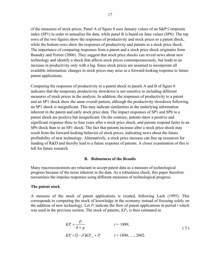
Many macroeconomists are reluctant to accept patent data as a measure of technological progress because of the noise inherent in the data. As a robustness check, this paper therefore reexamines the impulse responses using different measures of technological progress. The patent stock A measure of the stock of patent applications is created, following Lach (1995). This corresponds to computing the stock of knowledge in the economy instead of focusing solely on the addition of new technology. Let Pt indicate the flow of patent applications in period t which was used in the previous section. The stock of patents, KPt, is then estimated as

gPKP t

t +=δ

t = 1889,

( ) ttt PKPKP +−= −11 δ t = 1890, …, 2002.

( 5 )

18 δ indicates the rate of depreciation of patent capital and is set to 15%, a level that is common in the literature. g is the average growth rate of patent applications over the full sample. The patent stock is illustrated in figure 9 together with the flow of patents. When comparing the two series, it can be observed that the patent stock mainly differs from the data on the flow of patents by smoothing the series. The response of productivity after a shock to the stock of patents is shown in figure 1018. The impulse response function shows that the temporary negative effect on productivity remains. This result is also robust to changes in the depreciation rate, δ, which was varied in the interval δ ∈ [0 , 1]. Using the stock of patents as the measure of technology, the analysis finds that consumption responds positively, corresponding to the effect using data on the flow of patents. This response is therefore not shown. Since the results are unchanged when using the stock of patents, the paper chooses to return to the use of patent flows as the measure of technological change. Evidence from a Restricted Model The VAR above incorporates dynamics in the system by allowing lags of productivity to affect the flow of patents. However, from table 2 it can be concluded that productivity does not Granger cause patents. Allowing for these dynamics in the VAR may therefore result in an unnecessary degrees of freedom reduction and less precise parameter estimation. To take this issue into account, the paper follows the approach of Lach and Schankerman (1989), who use firm-level data to estimate the importance of shocks that affect R&D, investment, and the stock market rate of return. Following their procedure, this paper allows investment to help explain the variation in patents and productivity in the unrestricted system of equations. This section therefore allows for three different kinds of shocks to the system. Ignoring exogenous variables, the unrestricted system of equations looks as follows:

⎥⎥⎥

⎦

⎤

⎢⎢⎢

⎣

⎡+

⎥⎥⎥

⎦

⎤

⎢⎢⎢

⎣

⎡

⎥⎥⎥

⎦

⎤

⎢⎢⎢

⎣

⎡=

⎥⎥⎥

⎦

⎤

⎢⎢⎢

⎣

⎡

−

−

−

t

t

t

t

t

t

t

t

t

Ciyp

LBLBLBLBLBLBLBLBLB

iyp

τηε

1

1

1

333231

232221

131211

)()()()()()()()()(

( 6 )

where pt is the flow of patents at time t. yt indicates productivity, and it is investment. Bij(L) for i, j=1, …, 3 are polynomials in the lag-operator, L. Finally, εt, ηt, and τt, are orthogonal disturbance terms, where it must be determined how the shocks affect each equation. C is a matrix of coefficients.

18 When the patent stock is used as the measure of technology, the VAR is estimated using p = 6 lags as suggested by the AIC criterion. The LR and Hannan-Quinn (HR) criteria suggest using p = 5 lags. This does not change the result.

19 Following Lach and Schankerman (1989), this paper uses F-tests, corresponding to Granger Causality tests, as exclusion criteria in the system. The model is estimated equation by equation assuming trend-stationarity with breaks in trend as described earlier, and the F-tests are computed on the individual equations. The following steps test whether patents, productivity, and investment individually and collectively Granger cause each other. The steps can be explained as follows:

Step 1. H0: yt and it do not Granger cause pt, neither individually nor collectively. Step 2. H0: pt and it do not Granger cause yt, neither individually nor collectively. Step 3. H0: pt and yt do not Granger cause it, neither individually nor collectively. Table 4 shows the results of the tests.

From step 1, the paper concludes that lags of productivity and investment do not help predict current levels of the patent flow, whereas the tests in step 2 show that lags of both patents and productivity do have predictive power for current productivity. For investment, there is evidence that lags of investment are important for prediction. Furthermore, at the 10 percent level it is rejected that patents and productivity jointly can be dropped from the regression, although neither has explanatory power individually. Since the theoretical prior is that patents help predict investment, the paper chooses to include patents and productivity in the investment equation. Based on the results of the exclusion restrictions, the paper follows the recursive identification structure used for the VAR in section V.A to restrict the matrix C, such that it is lower triangular. Ignoring the constant and other exogenous variables, the restricted system of equations can then be written as

⎥⎥⎥

⎦

⎤

⎢⎢⎢

⎣

⎡

⎥⎥⎥

⎦

⎤

⎢⎢⎢

⎣

⎡+

⎥⎥⎥

⎦

⎤

⎢⎢⎢

⎣

⎡

⎥⎥⎥

⎦

⎤

⎢⎢⎢

⎣

⎡=

⎥⎥⎥

⎦

⎤

⎢⎢⎢

⎣

⎡

−

−

−

t

t

t

t

t

t

t

t

t

iyp

LBLBLBLBLB

LB

iyp

τηε

δβα

111000

)()()(0)()(00)(

1

1

1

333231

2221

11

, ( 7 )

where effects of the orthogonal disturbances on the endogenous variables are normalized in the it-equation, as indicated by the row of ones. The matrix of coefficients on the disturbance terms indicates the causal ordering by being lower triangular such that a shock to patents, εt, is allowed to have immediate effect on the remaining endogenous variables. The coefficient estimates of the endogenous variables in the restricted system are shown in table 5 together with standard errors of the estimates and the variance-covariance matrix of the residuals from the regressions, Σ̂ . It is important to note that the matrix of coefficients on lagged endogenous variables is lower triangular in this restricted system. This means that there is no feedback from changes in productivity to patents as was the case in the benchmark model in section V.A.

20 Since the residuals can be decomposed into orthogonal disturbance terms it is of interest to identify the effects that these orthogonal disturbances have on the endogenous variables. To do this, the symmetric variance-covariance matrix of the error terms is analytically solved as

⎥⎥⎥

⎦

⎤

⎢⎢⎢

⎣

⎡

++++=Σ

222222

22222

22

...

......

τηεηεε

ηεε

ε

σσσδσβσασσδσβαβσ

σα, ( 8 )

where 2

iσ is the variance of the orthogonal error term i, for i = ε, η, and τ. The 6 distinct elements of the variance-covariance matrix yield a system of 6 equations in 6 unknowns.19 Solving this system of equations allows the paper to find the coefficients on the shocks and the variances of the disturbances. Parameter estimates are given in table 6. Impulse response functions from the restricted model are then computed by simulation and shown in figure 11. It is confirmed that productivity responds negatively to the arrival of new technology as a shock to εt, which is the shock associated with the flow of patents, leads to a decrease in productivity. The paper therefore concludes that the results are robust to restricting the system in order to obtain more precise parameter estimates. Research and Development R&D expenditures, which are an input to the production of new technologies, precede any future patents and may lead to inventions that are not patented. It is therefore of interest to see how productivity responds to an R&D shock. For this analysis, the paper uses data on investment in privately financed R&D for the period 1935–199720. The resulting impulse response functions from a trivariate VAR with R&D, patents, and productivity are shown in figure 12. As theory predicts, the system shows that patents indeed increase significantly after an R&D shock and that productivity responds negatively in the short run. However, an interesting feature of the impulse response of productivity to an R&D shock is the positive effect after around 7 years. This is likely due to leaving out the relatively slow rate of diffusion of products during the Electrification period in the beginning of the 20th century. Using R&D data over the period 1935–1997, when the speed of diffusion tended to be faster, makes it possible to identify the eventual positive effects of new technology on productivity. That the time period is important can also be seen from the corresponding response of productivity to a patent shock in figure 12. This figure shows a response similar to what is

19 The 6 unknowns are the three parameters, α, β, and δ, together with the three variances of the orthogonal disturbance terms, 2

εσ , 2ησ , and 2

τσ .

20 Data on R&D for 1997 are an estimated value. The results are robust to ending the R&D sample in 1996. A dummy for WWII is left out in this subsection, as the number of observations is smaller.

21 observed with an R&D shock.21 The equivalent responses from a bivariate VAR (not shown) with either patents or R&D and productivity for the period 1935–1997 show similar responses. That is, patent data succeed in identifying the initial short-run response and the future positive response. The paper concludes that the results are robust to using different measures of technology. The observation that VARs, using either R&D data or patent data, produce equivalent impulse responses supports the validity of patent data as a measure of technological progress. However, the fact that impulse response functions based on the sample period 1935–1997 show a different pattern than when based on the full sample indicates the importance of further analysis of sub-samples of the data. The pre-IT period One can argue that the increase in the rate of patenting after 1985 explains a large part of the result since productivity growth was relatively low around this period. The estimations were therefore repeated, leaving out the period 1986–2002. This did not change the conclusions but only yielded a further negative response of productivity to a patent shock and consumption still exhibited a temporary increase after a patent shock. However, the initial response of investment was muted and became negative after a few years, matching the negative response of output. Overall, limiting the analysis to the period before the surge in patenting in 1985 and thereby only including the pre-Information Technology (IT) period does not change the conclusions but only renders responses of productivity to technology shocks that are more negative. The fact that the response of investment is more negative while the data show a longer-lasting slowdown in productivity when considering the pre-IT period may indicate that the faster rates of diffusion in the last part of the 20th century may be very important for understanding and identifying any economic contractionary or expansionary effects of new technology. This is so, because the more negative response of investment in the early period is an indication of slow diffusion where firms postpone investments until the new technology has been further improved. As seen in figure 5, the rate of adoption of electricity among American households was slower than the equivalent adoption rate for the internet. This paper therefore now considers any possible differences between the pre-WWII and the post-WWII periods.

VI. PRE- AND POST-WWII

The sample is now divided into two sub-periods. The pre-WWII period covers the years 1889–1940 while the post-WWII period extends over 1948–2002. Doing this allows technological progress to affect productivity differently during the Electrification period, when the diffusion of technology was relatively slow, than during the IT period, when diffusion happened more rapidly.

21 The trivariate VAR was estimated under several different specifications for the ordering of the variables. The resultant responses look similar to the ones illustrated in figure 12 and are therefore not reported.

22 The Electrification period was a period over more than 30 years and was a period during which several important GPTs were invented and implemented. Because of the relatively slow rate of diffusion for electricity, it is very likely that learning and reorganization processes within firms were relatively long lasting, leading to more pronounced negative effects on productivity in the pre-WWII period than in the post-WWII period. For the IT period, adoption of the internet started immediately after the invention in 1991 and the speed of diffusion was fast already from the beginning. Therefore, one should expect shorter-lasting negative effects on the macro economy since any positive network externalities will arrive faster with a high rate of diffusion relative to a slow diffusion process. A further argument for dividing the data into two periods, before and after WWII, is the change in volatility. Figure 2, panel B, shows how productivity growth exhibited larger volatility in the pre-WWII period where the standard deviation of the growth rate is 0.039, than after WWII, where the standard deviation is merely 0.016. Similarly is it the case for the growth rate in patent applications which also experienced a decrease in the variance after WWII.

A. VAR Estimation on Two Sample Periods

The impulse response functions from a bivariate VAR with patents and productivity in the two sub-samples are shown in figure 13. For both the pre- and the post-WWII periods the AIC suggests using p = 1 lag. However, because of the slow diffusion of technology during the early period, more lags may be needed. The figure therefore also shows the response functions using 4 lags. As seen, the response functions are robust to using different lag lengths. The difference between the two periods is easily seen. In the pre-war period, productivity depicts the temporary slowdown as seen when using the full sample. On the contrary, in the post-war period, there is no evidence of a temporary slowdown. Instead, the positive effects of a technology shock are now prevalent such that productivity increases significantly after 2-3 years. Including more lags in the estimation postpones the significantly positive effect another couple of years but without evidence of a productivity slowdown. This result is very important for understanding the productivity slowdown during the Electrification period and after 1973. The paper finds evidence that technology, indeed, can lead to a temporary productivity slowdown as seen in the early period. However, from this analysis it can be concluded that the productivity slowdown after 1973 does not seem to be a result of the arrival of new technology. In panel A of figure 13 with pre-WWII data, the long-run positive effects of technological progress on productivity do not show up when using 1 or 4 lags. This may be due to only considering a sub-sample period when diffusion was considerably slow. Figure 13, panel A, therefore also estimates the VAR using 9 lags. This consumes many degrees of freedom but may provide an indication that the long diffusion lags are important. Indeed, when including more than 8 lags the future positive effects do show up in the long run, although insignificantly, while still depicting a temporary slowdown in the short run.

For the pre-WWII period, responses of other variables than productivity look similar to the responses using the entire sample period and are therefore not reported. For the post-WWII period there are important differences that must be further analyzed. The following therefore focuses on the post-WWII period which can yield important insights for the current literature.

23

B. Post-WWII VECM

If there is evidence of cointegrating relationships when considering the post-WWII period separately, a vector error-correction model (VECM) may provide a better description of the data than stationarity around a deterministic trend with breaks. Furthermore, the inclusion of a break in trend in the regressions may partly explain the lack of a productivity slowdown in the later period. It is therefore of interest to examine the system of equations without exogenously removing the 1973 trend break. When looking at the full sample period and at the pre-WWII period only, there is no evidence of cointegration and the results are robust to different specifications. However, cointegrating relationships for the post-WWII period cannot be rejected at a 5 percent level. Results from a cointegration test in the bivariate system for this period are reported in panel A of table 7 and panel B reports corresponding tests in trivariate systems. At a 5 percent level, the paper cannot reject one cointegrating relationship in the system. This section therefore examines the responses to a patent shock under the assumption that a VECM best describes the post-WWII data. Impulse response functions with 95 percent confidence intervals calculated by Hall Bootstrap22 methods are reported in figure 14. Panel A of this figure illustrates the responses of patents and productivity to a patent shock in a bivariate VECM. Each row in panel B depicts responses to a patent shock, based on a VECM with three variables where the third variable changes, according to the measure of interest. Lag length is determined mainly based on AIC estimates. The corresponding VARs without imposing cointegrating relations and without deterministic trends in the regressions are also estimated in figure 15.23 Figure 15, panel A, reports the impulse response functions from a bivariate VAR with patents and productivity. Panel B of figure 15 reports the equivalent responses from trivariate VARs. The organization of the variables corresponds to the ordering from the VECM analysis. The responses for productivity, consumption, investment, and output, as measured by GDP, generally show equivalent pictures whether estimated from a VECM or a VAR. Figure 14, panel A, with VECM results reports that labor productivity does not display a significant slowdown after a patent shock but that productivity increases significantly after several years. In figure 14, panel B, consumption increases slowly but the response remains statistically indistinguishable from zero at a 5 percent level. However, the corresponding VAR with no cointegration in figure 15, panel B, does depict a significant response. Investment and output slowly converge to a significantly higher level. When based on a VECM, hours do not show a significant response but do indicate that labor input use is reduced in the long run after the arrival of new technology. However, when estimating the response of hours based on a VAR with no cointegration, as illustrated in panel B of figure 15, hours do not demonstrate a reduction in input use in the long run. If hours are truly constant, such that long-run labor input use is unchanged after the arrival of new technology, then the post-WWII impulse response

22 Efron bootstrap confidence intervals were also computed. Hall confidence intervals tend to show more significant results than Efron estimates. However, the overall conclusions derived from impulse response functions using these confidence intervals were unchanged.

23 Impulse responses with trend and break (not shown) depict responses that lead to unchanged conclusions.

24 functions can be matched by a standard growth model with labor held constant, assuming that technology arrives exogenously through slow diffusion. The theoretical implications will be discussed in section VII. The VECM analysis confirms results from the previous section, that there is not evidence of a significant slowdown in the post-WWII period after the arrival of new technology. That any transitory contractionary effects of a new invention are more prevalent in the pre-war period indicates the importance of further analysis of the consequence of the rate of diffusion and learning for the economic effects. It is left for future research to explore these differences in more thorough detail. Instead, the paper now estimates the importance of technology shocks for variations in productivity at different horizons.

C. Variance Decomposition

In the neoclassical models, a large focus has been put on the role of technological progress. Using the historical data in this paper, it is possible to estimate the importance of a patent shock for the variation in productivity. Table 8, panel A, shows the results from a decomposition of the forecast error variance during the two sub-sample periods under different assumptions about the data in a bivariate analysis with patents and productivity. Panel B of table 8 reports results using R&D as a measure of technology instead of patents and panel C displays the results if a third variable is included in the system. In the period 1889–1940, 37 percent of the variation in productivity can be explained by the patent shock at a 50 year horizon. Similarly, in the post-WWII period 61.5 percent of the variation is explained by the technology shock when estimating in a VAR with deterministic trend assumptions but almost 90 percent is explained when taking into account possible cointegration during the sample period. These numbers indicate that patents explain a large fraction of long-run variation in productivity and that patent data therefore do capture the arrival of new technology. As a result, the paper concludes that technology shocks, indeed, are important for fluctuations in productivity. Equivalently, R&D explains around 27 percent of the variation in productivity. However, in the case of R&D, the sample period includes the war time years. Generally, technology shocks, identified with patents, seem to explain a larger fraction of the variance of productivity in the post-war period than in the earlier period. However, the estimates in table 8 are smaller than the results computed by Francis and Ramey (2004). Through a long-run specification, they find that technology shocks explain more than 90 percent of the variance of productivity on a horizon longer than three years. That patents only account for up to 90 percent of the forecast error variance of productivity at a horizon of 50 years is an indication that also other sources than technology are important for explaining long-run fluctuations in productivity. It is therefore likely that human capital can be important, also in the long run, when explaining fluctuations in productivity growth. Many economists focus mainly on determining the effects of new technology on productivity at a business cycle horizon. As an example, Beaudry and Portier (2006) have argued that news about future technology can lead to an economic expansion in the short run. However, the

25 variance decomposition in table 8 illustrates that the arrival of new technology as measured by new patent applications only have little importance for the variation in productivity at a horizon shorter than three years. After five years, approximately 24 percent of the variation in productivity is explained by patents in the pre-WWII period while around 18 percent of the variation is explained in the post-WWII period when estimating with a VAR. To further explore the importance of technology shocks at the business cycle horizon, table 8, panel C, reports the variance decomposition results for the post-WWII period when based on a trivariate system. The table shows that technology shocks alone are not important for explaining business cycle fluctuations since less than seven percent of the variation is explained by patents at a horizon shorter than five years. However, technology is important for explaining variations in investment and output in the long run. Furthermore, when consumption, output, or hours worked are included in the system, the variation in productivity explained by patents at a horizon of 50 years remains around 90 percent when estimated by a VECM (not shown) and the overall conclusions are not sensitive to the ordering of the variables in the systems.

VII. THEORETICAL IMPLICATIONS OF THE RESULTS

The main purpose of this paper is to provide empirical, statistical evidence for how the economy responds to the arrival of new technology. However, the result that technology shocks are not important for explaining business cycle expansions has important implications for current theoretical macroeconomic research. The real business cycle model predicts that a technology shock has an immediate and positive impact on the economy. However, from the present analysis, this paper concludes that this result does not match the data. The next important step is therefore to explore which models can explain these empirical findings. The post-WWII response functions point in the direction of incorporating slow diffusion when modeling technological progress. A model with a continuum of plants that adopt the new technology at different times is therefore an appropriate setting for incorporating slow diffusion. Rotemberg (2003) has a model which incorporates the diffusion of technological innovations that can lead to temporary slowdowns in output. However, this coincides with fluctuations in hours worked that do not correspond to the present empirical findings. Therefore, an S-shaped adoption rate cannot alone explain the empirical results. The pre-WWII period is not only affected by slow diffusion but also by temporary adverse effects that significantly decrease labor productivity. One promising line of research is therefore to explore the importance of learning and the influence of the stock of human capital that may facilitate the adoption of new technology. On this issue, Bartel (1989) showed that large businesses that are introducing new technologies are more likely to have formal training programs and that formal training of workers have a positive impact on productivity. Therefore, more skilled labor in the post-1948 period compared to the early part of the sample may enable easier and faster learning and thereby shorten the time-lag until any positive effects show up in the productivity data. This is also evidenced by Bartel and Sicherman (1999) who confirm that workers in industries with higher rates of technological change have more human capital. Compatibility problems between old and new technologies may also play a role in the early part of the sample and including such factors may improve the performance of a theoretical model explaining the effects of technological progress on productivity over long sample periods.

26

VIII. CONCLUSION

This paper has argued that patent application data can be used as a valid measure of technological progress. Using vector autoregressions on data from 1889 to 2002, this paper concludes that when examining the full sample period aggregate labor productivity responds negatively in the short run after technological progress occurs. This result is robust to several different methodological specifications and to utilizing the stock of patent applications and R&D data as alternative measures of technology. The paper found evidence that the effects of technology shocks on productivity have changed substantially over the last century. This may be a result of changes in the rate of diffusion of technology since diffusion has been faster in the post-WWII period than it was in the pre-WWII era. A faster rate of diffusion can lead to shorter-lasting negative effects of technology shocks, and future positive effects on productivity will then show up in the impulse response functions. The effect of human capital may also be very important since more skilled labor facilitates the adoption of new technology. That there are important changes over the sample period is indeed what the data demonstrate. Using data from 1889–1940, productivity is estimated to be lower than the initially forecasted level following a technology shock, after which it slowly reverts back to the initial forecast and a further increase. On the contrary, data on 1948–2002 do not show significant negative effects on productivity. Instead, significantly positive revisions in the forecast are observed. Similarly, investment and output follow a path equivalent to that of productivity. Further examination of the importance of the rate of diffusion and the amount of skilled labor for the response of labor productivity to a technology shock is a subject for future research. Variance decompositions support the role of patent statistics as a measure of technological progress since variations in long-run productivity are explained mainly by patents. However, the analysis also shows that technology shocks are not very important in explaining business cycle fluctuations. The empirical findings in this paper therefore have important theoretical implications. The results point toward the importance of incorporating slow diffusion, human capital, and learning in macroeconomic models when trying to understand the effects of technological progress on productivity.

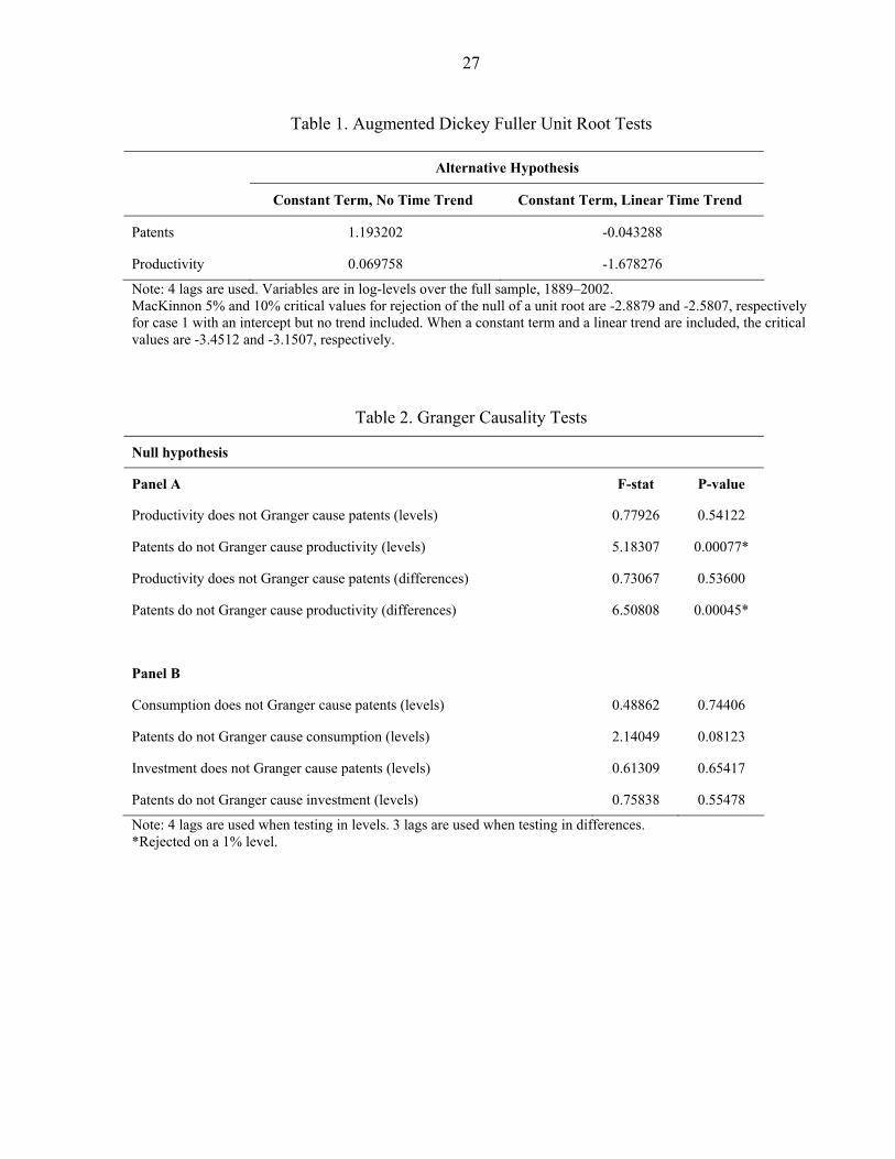
27

Table 1. Augmented Dickey Fuller Unit Root Tests

Alternative Hypothesis

Constant Term, No Time Trend Constant Term, Linear Time Trend

Patents 1.193202 -0.043288

Productivity 0.069758 -1.678276

Note: 4 lags are used. Variables are in log-levels over the full sample, 1889–2002. MacKinnon 5% and 10% critical values for rejection of the null of a unit root are -2.8879 and -2.5807, respectively for case 1 with an intercept but no trend included. When a constant term and a linear trend are included, the critical values are -3.4512 and -3.1507, respectively.

Table 2. Granger Causality Tests

Null hypothesis

Panel A F-stat P-value

Productivity does not Granger cause patents (levels) 0.77926 0.54122

Patents do not Granger cause productivity (levels) 5.18307 0.00077*

Productivity does not Granger cause patents (differences) 0.73067 0.53600

Patents do not Granger cause productivity (differences) 6.50808 0.00045*

Panel B

Consumption does not Granger cause patents (levels) 0.48862 0.74406

Patents do not Granger cause consumption (levels) 2.14049 0.08123

Investment does not Granger cause patents (levels) 0.61309 0.65417

Patents do not Granger cause investment (levels) 0.75838 0.55478

Note: 4 lags are used when testing in levels. 3 lags are used when testing in differences. *Rejected on a 1% level.

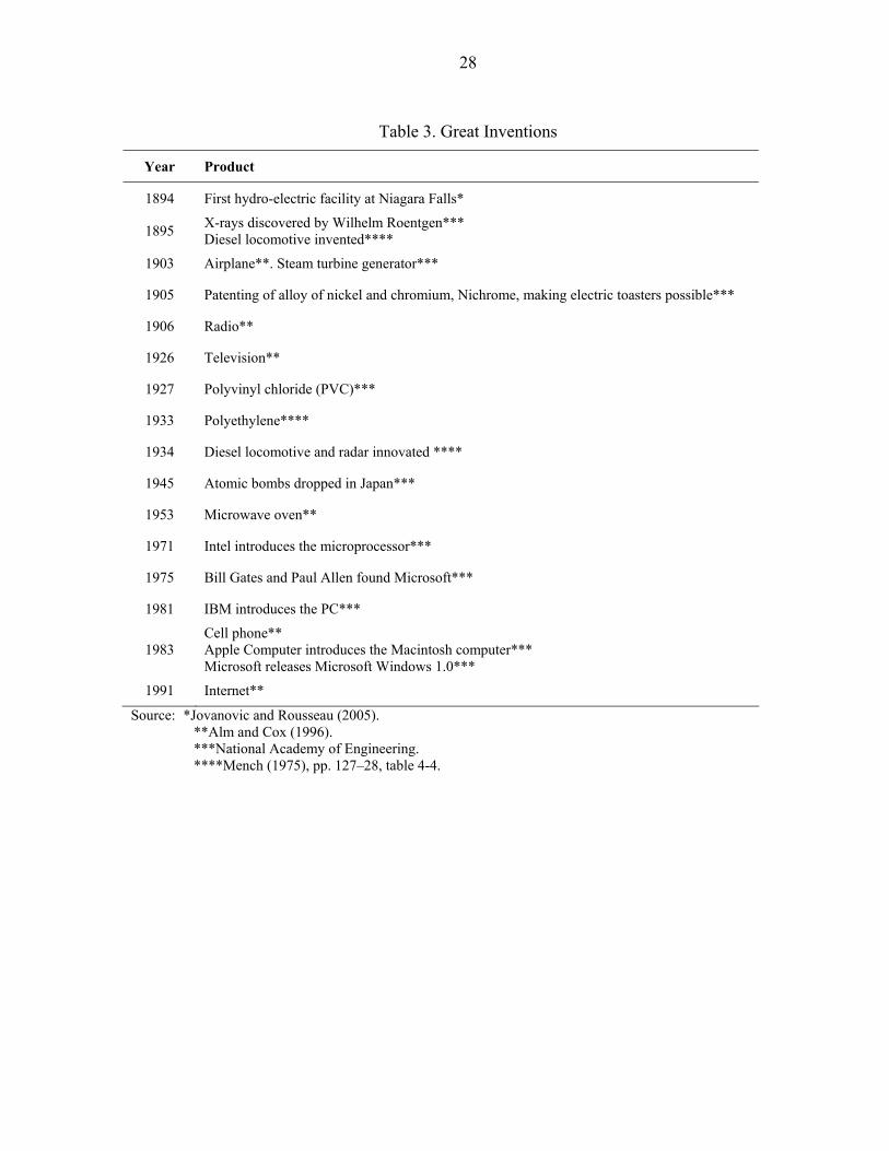
28

Table 3. Great Inventions

Year Product

1894 First hydro-electric facility at Niagara Falls*

1895 X-rays discovered by Wilhelm Roentgen*** Diesel locomotive invented****

1903 Airplane**. Steam turbine generator***

1905 Patenting of alloy of nickel and chromium, Nichrome, making electric toasters possible***

1906 Radio**

1926 Television**

1927 Polyvinyl chloride (PVC)***

1933 Polyethylene****

1934 Diesel locomotive and radar innovated ****

1945 Atomic bombs dropped in Japan***

1953 Microwave oven**

1971 Intel introduces the microprocessor***

1975 Bill Gates and Paul Allen found Microsoft***

1981 IBM introduces the PC***

1983 Cell phone** Apple Computer introduces the Macintosh computer*** Microsoft releases Microsoft Windows 1.0***

1991 Internet**

Source: *Jovanovic and Rousseau (2005). **Alm and Cox (1996). ***National Academy of Engineering. ****Mench (1975), pp. 127–28, table 4-4.

29

Table 4. Exclusion Tests in a Restricted Model

Null hypothesis F-statistic P-value

Step 1 (pt) pt does not Granger Cause pt 54.02592 0.000000

Step 1 (yt) yt does not Granger Cause pt 1.236390 0.300998

Step 1 (it) it does not Granger Cause pt 1.910400 0.115306

Step 1 (yt and it) yt and it do not Granger Cause pt 1.367494 0.221240

Step 2 (pt) pt does not Granger Cause yt 3.544856 0.009778

Step 2 (yt) yt does not Granger Cause yt 42.12399 0.000000

Step 2 (it) it does not Granger Cause yt 0.581868 0.676527

Step 2 (pt and it) it and pt do not Granger Cause yt 2.544901 0.014986

Step 3 (pt) pt does not Granger Cause it 0.881667 0.478175

Step 3 (yt) yt does not Granger Cause it 1.201055 0.315762

Step 3 (it) it does not Granger Cause it 5.888828 0.000290

Step 3 (pt and yt) pt and yt do not Granger Cause it 1.939921 0.063181

Note: 4 lags are used. A time trend, a change in the intercept in 1930, a break in trend in 1973, and dummies for the Great Depression and WWII are included.

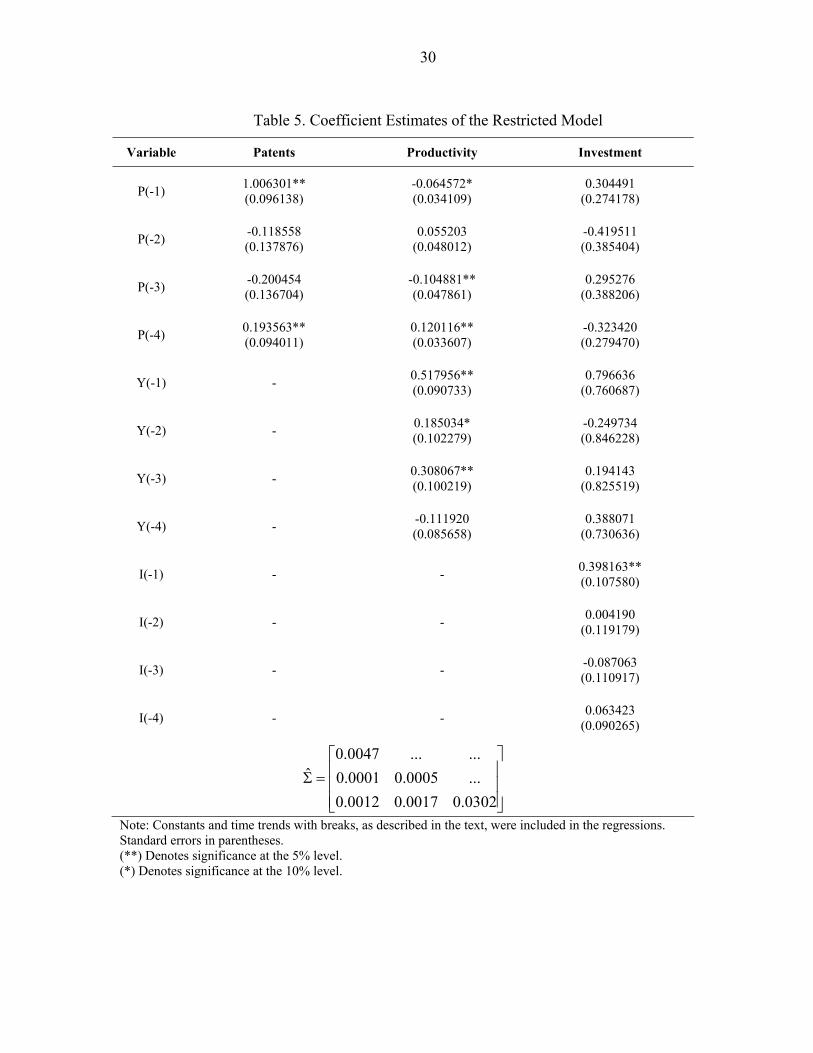
30

Table 5. Coefficient Estimates of the Restricted Model

Variable Patents Productivity Investment

P(-1) 1.006301** (0.096138)

-0.064572* (0.034109)

0.304491 (0.274178)

P(-2) -0.118558 (0.137876)

0.055203 (0.048012)

-0.419511 (0.385404)

P(-3) -0.200454 (0.136704)

-0.104881** (0.047861)

0.295276 (0.388206)

P(-4) 0.193563** (0.094011)

0.120116** (0.033607)

-0.323420 (0.279470)

Y(-1) - 0.517956** (0.090733)

0.796636 (0.760687)

Y(-2) - 0.185034* (0.102279)

-0.249734 (0.846228)

Y(-3) - 0.308067** (0.100219)

0.194143 (0.825519)

Y(-4) - -0.111920 (0.085658)

0.388071 (0.730636)

I(-1) - - 0.398163** (0.107580)

I(-2) - - 0.004190 (0.119179)

I(-3) - - -0.087063 (0.110917)

I(-4) - - 0.063423 (0.090265)

⎥⎥⎥

⎦

⎤

⎢⎢⎢

⎣

⎡=Σ

0302.00017.00012.0...0005.00001.0......0047.0

ˆ

Note: Constants and time trends with breaks, as described in the text, were included in the regressions. Standard errors in parentheses. (**) Denotes significance at the 5% level. (*) Denotes significance at the 10% level.

31

Table 6. Parameter Estimates for the Restricted Model

Parameter Value Parameter Value

α 3.9167 2εσ 0.0003

β 0.0833 2ησ 0.0056

δ 0.2973 2τσ 0.0243

Table 7. Cointegration in Post-WWII Data

Hypothesized number of cointegrating relations Trace Statistic 5 percent critical value 1 percent critical value

Panel A. Bivariate system

Patents and Productivity: 0 22.57 15.41 20.04

At most 1 3.53 3.76 6.65

Panel B. Trivariate systems

Consumption: 0 36.06 29.68 35.65

At most 1 9.56 15.41 20.04

Investment: 0 35.13 29.68 35.65

At most 1 15.34 15.41 20.04

Output: 0 36.21 29.68 35.65

At most 1 8.38 15.41 20.04

Hours: 0 34.94 29.68 35.65

At most 1 8.41 15.41 20.04 Note: The test allows for a linear deterministic trend in data. 1 lag in differences is included. The paper only shows results for up to 1 cointegrating relation since this is accepted.

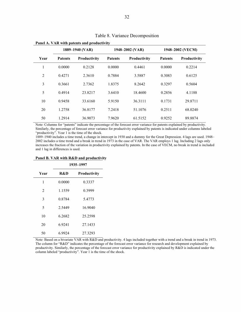
32

Table 8. Variance Decomposition

Panel A. VAR with patents and productivity

1889–1940 (VAR) 1948–2002 (VAR) 1948–2002 (VECM)

Year Patents Productivity Patents Productivity Patents Productivity

1 0.0000 0.2128 0.0000 0.4461 0.0000 0.2214

2 0.4271 2.3610 0.7884 3.5887 0.3083 0.6125

3 0.3661 2.7362 1.8375 8.2642 0.3297 0.5604

5 0.4914 23.8217 3.6410 18.4600 0.2856 4.1188

10 0.9458 33.6160 5.9150 36.3111 0.1731 29.8711

20 1.2758 36.8177 7.2418 51.1076 0.2511 68.0240

50 1.2914 36.9073 7.9620 61.5152 0.9252 89.8874 Note: Columns for “patents” indicate the percentage of the forecast error variance for patents explained by productivity. Similarly, the percentage of forecast error variance for productivity explained by patents is indicated under columns labeled “productivity”. Year 1 is the time of the shock. 1889–1940 includes a time trend, a change in intercept in 1930 and a dummy for the Great Depression. 4 lags are used. 1948–2002 includes a time trend and a break in trend in 1973 in the case of VAR. The VAR employs 1 lag. Including 2 lags only increases the fraction of the variation in productivity explained by patents. In the case of VECM, no break in trend is included and 1 lag in differences is used. Panel B. VAR with R&D and productivity

1935–1997

Year R&D Productivity

1 0.0000 0.3337

2 1.1559 0.3999

3 0.8784 5.4773

5 2.5449 16.9040

10 6.2682 25.2598

20 6.9241 27.1433

50 6.9924 27.3293 Note: Based on a bivariate VAR with R&D and productivity. 4 lags included together with a trend and a break in trend in 1973. The column for “R&D” indicates the percentage of the forecast error variance for research and development explained by productivity. Similarly, the percentage of the forecast error variance for productivity explained by R&D is indicated under the column labeled “productivity”. Year 1 is the time of the shock.

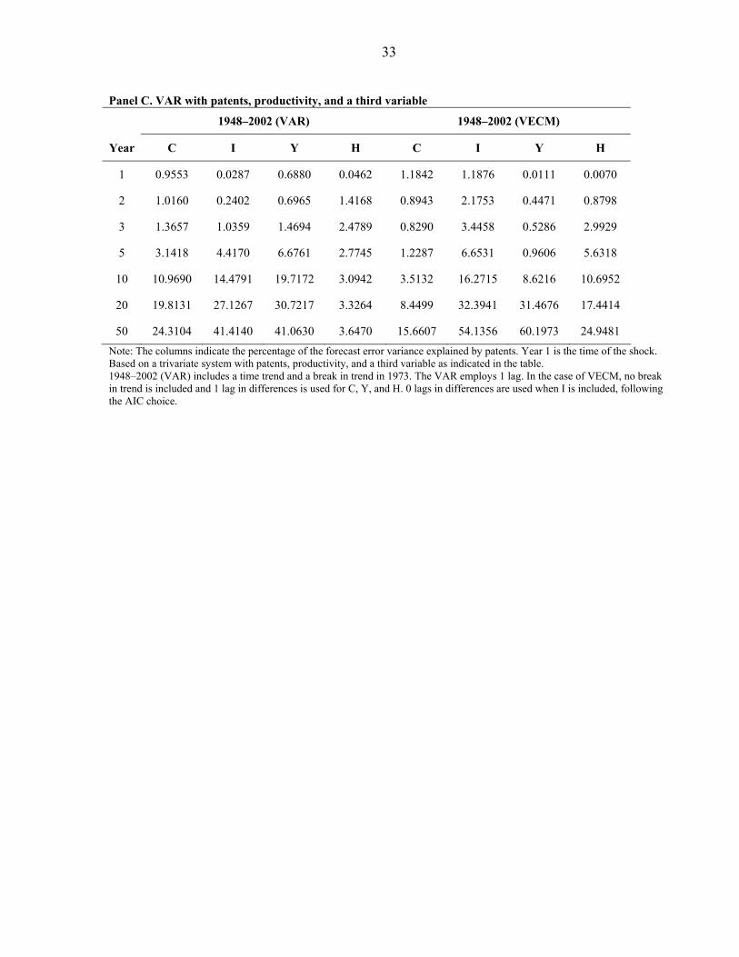
33 Panel C. VAR with patents, productivity, and a third variable

1948–2002 (VAR) 1948–2002 (VECM)

Year C I Y H C I Y H

1 0.9553 0.0287 0.6880 0.0462 1.1842 1.1876 0.0111 0.0070

2 1.0160 0.2402 0.6965 1.4168 0.8943 2.1753 0.4471 0.8798

3 1.3657 1.0359 1.4694 2.4789 0.8290 3.4458 0.5286 2.9929

5 3.1418 4.4170 6.6761 2.7745 1.2287 6.6531 0.9606 5.6318

10 10.9690 14.4791 19.7172 3.0942 3.5132 16.2715 8.6216 10.6952

20 19.8131 27.1267 30.7217 3.3264 8.4499 32.3941 31.4676 17.4414

50 24.3104 41.4140 41.0630 3.6470 15.6607 54.1356 60.1973 24.9481 Note: The columns indicate the percentage of the forecast error variance explained by patents. Year 1 is the time of the shock. Based on a trivariate system with patents, productivity, and a third variable as indicated in the table. 1948–2002 (VAR) includes a time trend and a break in trend in 1973. The VAR employs 1 lag. In the case of VECM, no break in trend is included and 1 lag in differences is used for C, Y, and H. 0 lags in differences are used when I is included, following the AIC choice.

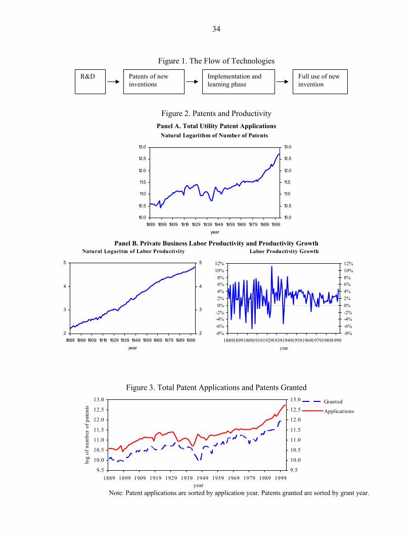
34

Figure 1. The Flow of Technologies

Figure 2. Patents and Productivity

Panel A. Total Utility Patent Applications

Panel B. Private Business Labor Productivity and Productivity Growth

Figure 3. Total Patent Applications and Patents Granted

Note: Patent applications are sorted by application year. Patents granted are sorted by grant year.

R&D Patents of new inventions

Implementation and learning phase

Full use of new invention

Natural Logarithm of Number of Patents

10.0

10.5

11.0

11.5

12.0

12.5

13.0

1889 1899 1909 1919 1929 1939 1949 1959 1969 1979 1989 1999

year

10.0

10.5

11.0

11.5

12.0

12.5

13.0

Natural Logaritm of Labor Productivity

2

3

4

5

1889 1899 1909 1919 1929 1939 1949 1959 1969 1979 1989 1999

year

2

3

4

5

Labor Productivity Growth

-8%-6%-4%-2%0%2%4%6%8%

10%12%

188918991909191919291939194919591969197919891999year

-8%-6%-4%-2%0%2%4%6%8%10%12%

9.5

10.0

10.5

11.0

11.5

12.0

12.5

13.0

1889 1899 1909 1919 1929 1939 1949 1959 1969 1979 1989 1999year

log

of n

umbe

r of p

aten

ts

9.5

10.0

10.5

11.0

11.5

12.0

12.5

13.0 Granted

Applications

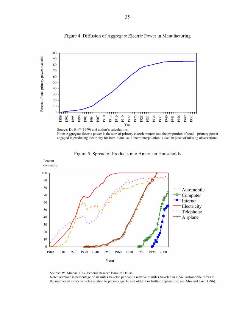
35

Figure 4. Diffusion of Aggregate Electric Power in Manufacturing

Source: Du Boff (1979) and author’s calculations. Note: Aggregate electric power is the sum of primary electric motors and the proportion of total primary power

engaged in producing electricity for intra-plant use. Linear interpolation is used in place of missing observations.

Figure 5. Spread of Products into American Households

Source: W. Michael Cox, Federal Reserve Bank of Dallas. Note: Airplane is percentage of air miles traveled per capita relative to miles traveled in 1996. Automobile refers to the number of motor vehicles relative to persons age 16 and older. For further explanation, see Alm and Cox (1996).

0 10 20 30 40 50 60 70 80 90

100

1900 1910 1920 1930 1940 1950 1960 1970 1980 1990 2000

Year

Percentownership

AutomobileComputerInternetElectricityTelephoneAirplane

0

10

20

30

40

5060

70

80

90

100

1889

1892

1895

1898

1901

1904

1907

1910

1913

1916

1919

1922

1925

1928

1931

1934

1937

1940

1943

1946

1949

1952

Year

Perc

ent o

f tot

al p

rimar

y po

wer

ava

ilabl

e

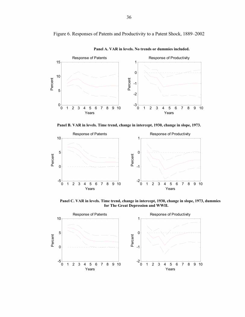
36

Figure 6. Responses of Patents and Productivity to a Patent Shock, 1889–2002

Panel A. VAR in levels. No trends or dummies included.

0 1 2 3 4 5 6 7 8 9 100

5

10

15Response of Patents

Per

cent

Years0 1 2 3 4 5 6 7 8 9 10

-3

-2

-1

0

1Response of Productivity

Per

cent

Years

Panel B. VAR in levels. Time trend, change in intercept, 1930, change in slope, 1973.

0 1 2 3 4 5 6 7 8 9 10-5

0

5

10Response of Patents

Per

cent

Years0 1 2 3 4 5 6 7 8 9 10

-2

-1

0

1Response of ProductivityP

erce

nt

Years

Panel C. VAR in levels. Time trend, change in intercept, 1930, change in slope, 1973, dummies

for The Great Depression and WWII.

0 1 2 3 4 5 6 7 8 9 10-5

0

5

10Response of Patents

Per

cent

Years0 1 2 3 4 5 6 7 8 9 10

-2

-1

0

1Response of Productivity

Per

cent

Years

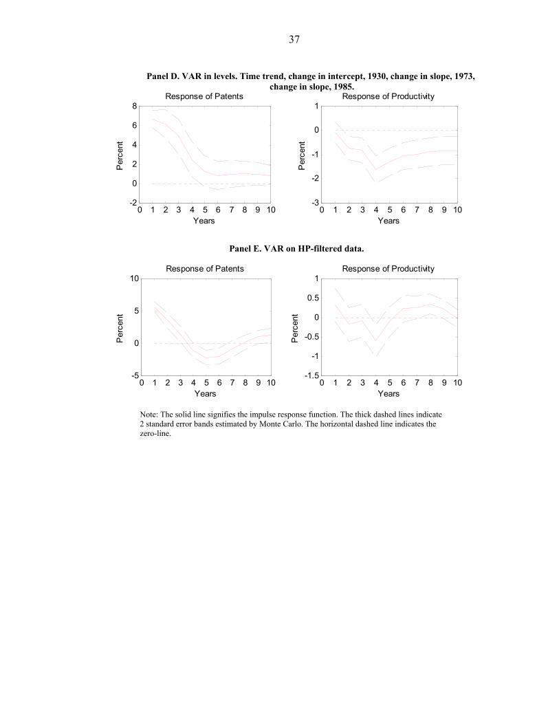
37

Panel D. VAR in levels. Time trend, change in intercept, 1930, change in slope, 1973, change in slope, 1985.

0 1 2 3 4 5 6 7 8 9 10-2

0

2

4

6

8Response of Patents

Per

cent

Years0 1 2 3 4 5 6 7 8 9 10

-3

-2

-1

0

1Response of Productivity

Per

cent

Years

Panel E. VAR on HP-filtered data.

0 1 2 3 4 5 6 7 8 9 10-5

0

5

10Response of Patents

Per

cent

Years0 1 2 3 4 5 6 7 8 9 10

-1.5

-1

-0.5

0

0.5

1Response of Productivity

Per

cent

Years

Note: The solid line signifies the impulse response function. The thick dashed lines indicate 2 standard error bands estimated by Monte Carlo. The horizontal dashed line indicates the zero-line.

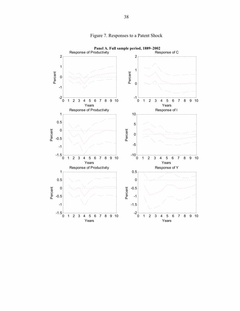
38

Figure 7. Responses to a Patent Shock

Panel A. Full sample period, 1889–2002

0 1 2 3 4 5 6 7 8 9 10-2

-1

0

1

2Response of Productivity

Per

cent

Years0 1 2 3 4 5 6 7 8 9 10

-1

0

1

2Response of C

Per

cent

Years

0 1 2 3 4 5 6 7 8 9 10-1.5

-1

-0.5

0

0.5

1Response of Productivity

Per

cent

Years0 1 2 3 4 5 6 7 8 9 10

-10

-5

0

5

10Response of I

Per

cent

Years

0 1 2 3 4 5 6 7 8 9 10-1.5

-1

-0.5

0

0.5

1Response of Productivity

Per

cent

Years0 1 2 3 4 5 6 7 8 9 10

-2

-1.5

-1

-0.5

0

0.5Response of Y

Per

cent

Years

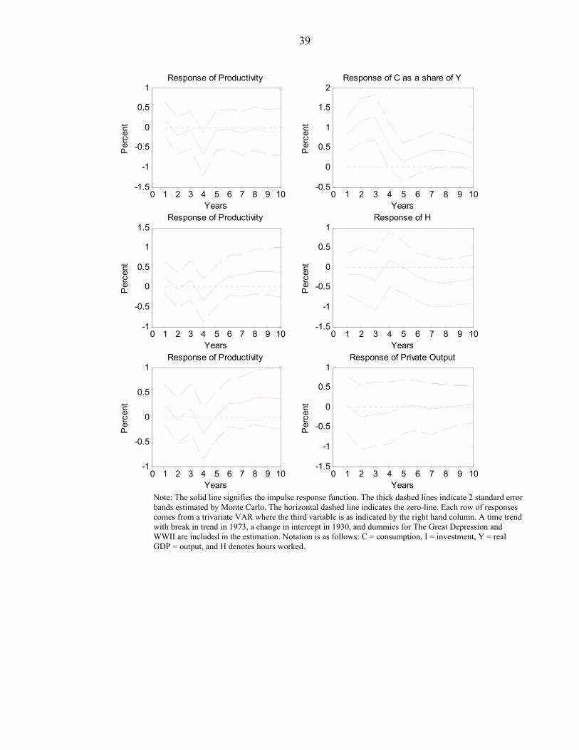
39

0 1 2 3 4 5 6 7 8 9 10-1.5

-1

-0.5

0

0.5

1Response of Productivity

Per

cent

Years0 1 2 3 4 5 6 7 8 9 10

-0.5

0

0.5

1

1.5

2Response of C as a share of Y

Per

cent

Years

0 1 2 3 4 5 6 7 8 9 10-1

-0.5

0

0.5

1

1.5Response of Productivity

Per

cent

Years0 1 2 3 4 5 6 7 8 9 10

-1.5

-1

-0.5

0

0.5

1Response of H

Per

cent

Years

0 1 2 3 4 5 6 7 8 9 10-1

-0.5

0

0.5

1Response of Productivity

Per

cent

Years0 1 2 3 4 5 6 7 8 9 10

-1.5

-1

-0.5

0

0.5

1Response of Private Output

Per

cent

Years Note: The solid line signifies the impulse response function. The thick dashed lines indicate 2 standard error bands estimated by Monte Carlo. The horizontal dashed line indicates the zero-line. Each row of responses comes from a trivariate VAR where the third variable is as indicated by the right hand column. A time trend with break in trend in 1973, a change in intercept in 1930, and dummies for The Great Depression and WWII are included in the estimation. Notation is as follows: C = consumption, I = investment, Y = real GDP = output, and H denotes hours worked.

40

Panel B. Shorter than full sample period

0 1 2 3 4 5 6 7 8 9 10-0.5

0

0.5

1Response of W

Per

cent

Years0 1 2 3 4 5 6 7 8 9 10

-1

0

1

2Response of Income

Per

cent

Years Note: The solid line signifies the impulse response function. The thick dashed lines indicate 2 standard error bands estimated by Monte Carlo. The horizontal dashed line indicates the zero-line. The response functions are from two different trivariate VARs. Data for wage inequality (W) cover the period 1927–1998. 4 lags are used. A time trend with break in trend is included together with dummies for WWII and 1987–88 and a change in intercept in 1945. Income inequality (Income) covers the period 1917–1998. 4 lags are used. A time trend with break in trend is included together with dummies for the Great Depression, WWII, and 1987–88 and changes in intercept in 1930 and 1945.

Figure 8: Stock prices, 1889–2002

Panel A. January values of stock prices

0 1 2 3 4 5 6 7 8 9 10-2

-1

0

1Response of Productivity to Patents

Per

cent

Years0 1 2 3 4 5 6 7 8 9 10

-10

-5

0

5

10Response of SP1 to Patents

Per

cent

Years

0 1 2 3 4 5 6 7 8 9 10-2

0

2

4

6Response of Patents to SP1

Per

cent

Years0 1 2 3 4 5 6 7 8 9 10

-1

-0.5

0

0.5

1

1.5Response of Productivity to SP1

Per

cent

Years Note: The solid line signifies the impulse response function. The thick dashed lines indicate 2 standard error bands estimated by Monte Carlo. The horizontal dashed line indicates the zero-line. The responses are from a VAR with patents, productivity, and stock prices. A time trend with break in trend in 1973, a change in intercept in 1930, and dummies for The Great Depression and WWII are included in the estimation. SP1 denotes January values of the stock price index.

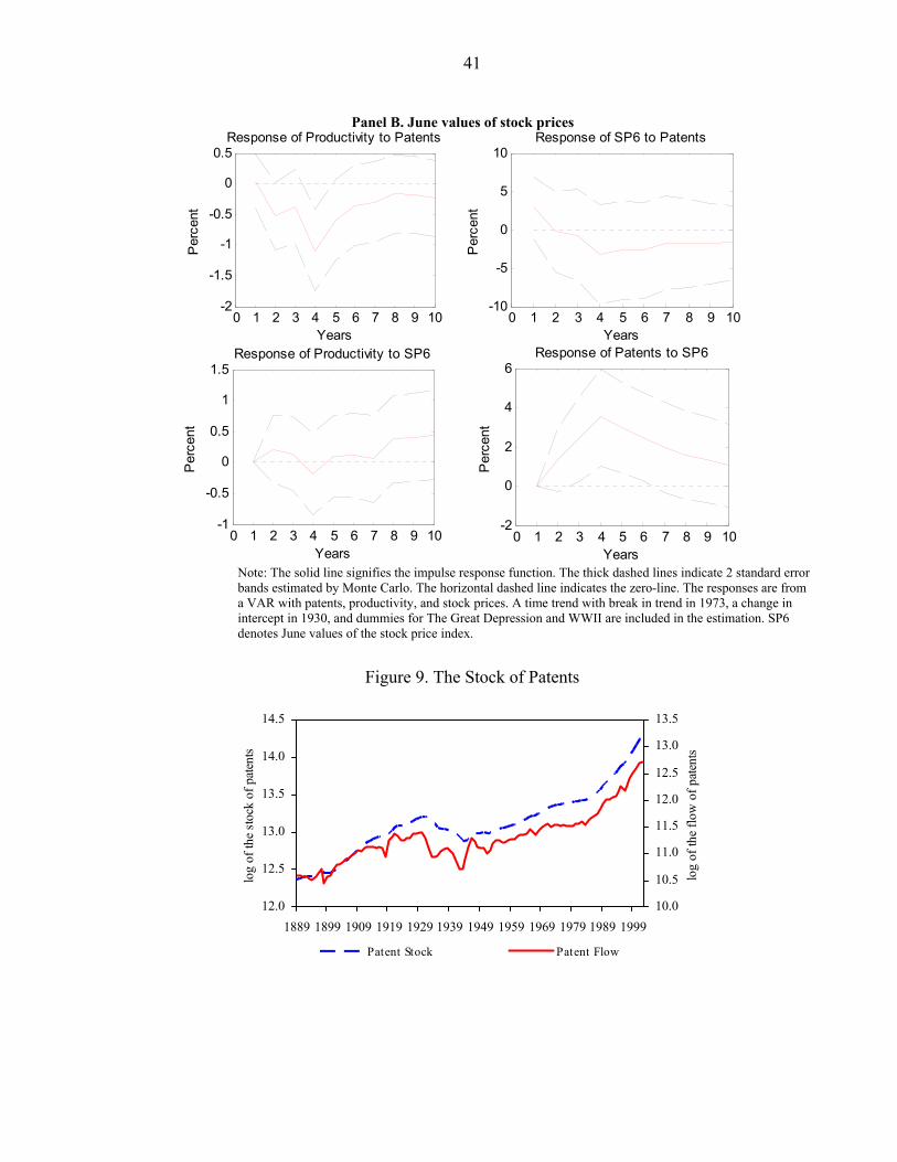
41

Panel B. June values of stock prices

0 1 2 3 4 5 6 7 8 9 10-2

-1.5

-1

-0.5

0

0.5Response of Productivity to Patents

Per

cent

Years0 1 2 3 4 5 6 7 8 9 10

-10

-5

0

5

10Response of SP6 to Patents

Per

cent

Years

0 1 2 3 4 5 6 7 8 9 10-2

0

2

4

6Response of Patents to SP6

Per

cent

Years0 1 2 3 4 5 6 7 8 9 10

-1

-0.5

0

0.5

1

1.5Response of Productivity to SP6

Per

cent

Years Note: The solid line signifies the impulse response function. The thick dashed lines indicate 2 standard error bands estimated by Monte Carlo. The horizontal dashed line indicates the zero-line. The responses are from a VAR with patents, productivity, and stock prices. A time trend with break in trend in 1973, a change in intercept in 1930, and dummies for The Great Depression and WWII are included in the estimation. SP6 denotes June values of the stock price index.

Figure 9. The Stock of Patents

12.0

12.5

13.0

13.5

14.0

14.5

1889 1899 1909 1919 1929 1939 1949 1959 1969 1979 1989 1999

year

log

of th

e st

ock

of p

aten

ts

10.0

10.5

11.0

11.5

12.0

12.5

13.0

13.5

log

of th

e flo

w o

f pat

ents

Patent Stock Patent Flow

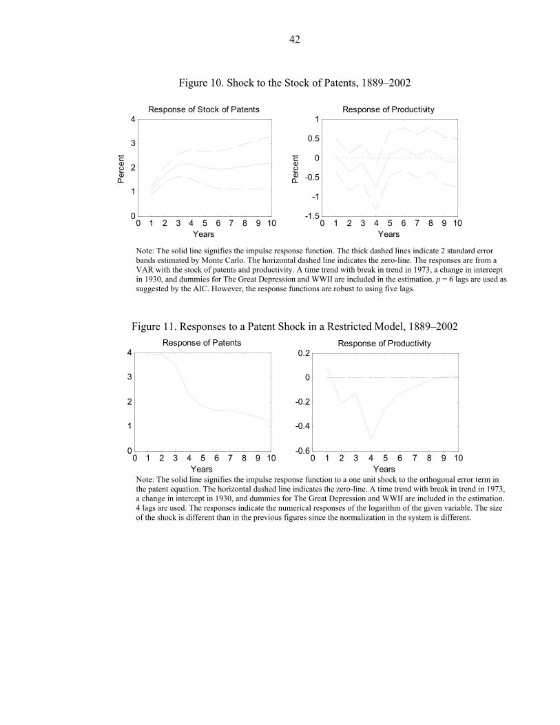
42

Figure 10. Shock to the Stock of Patents, 1889–2002

0 1 2 3 4 5 6 7 8 9 100

1

2

3

4Response of Stock of Patents

Per

cent

Years0 1 2 3 4 5 6 7 8 9 10

-1.5

-1

-0.5

0

0.5

1Response of Productivity

Per

cent

Years

Note: The solid line signifies the impulse response function. The thick dashed lines indicate 2 standard error bands estimated by Monte Carlo. The horizontal dashed line indicates the zero-line. The responses are from a VAR with the stock of patents and productivity. A time trend with break in trend in 1973, a change in intercept in 1930, and dummies for The Great Depression and WWII are included in the estimation. p = 6 lags are used as suggested by the AIC. However, the response functions are robust to using five lags.

Figure 11. Responses to a Patent Shock in a Restricted Model, 1889–2002

0 1 2 3 4 5 6 7 8 9 100

1

2

3

4Response of Patents

Years0 1 2 3 4 5 6 7 8 9 10

-0.6

-0.4

-0.2

0

0.2Response of Productivity

Years Note: The solid line signifies the impulse response function to a one unit shock to the orthogonal error term in the patent equation. The horizontal dashed line indicates the zero-line. A time trend with break in trend in 1973, a change in intercept in 1930, and dummies for The Great Depression and WWII are included in the estimation. 4 lags are used. The responses indicate the numerical responses of the logarithm of the given variable. The size of the shock is different than in the previous figures since the normalization in the system is different.

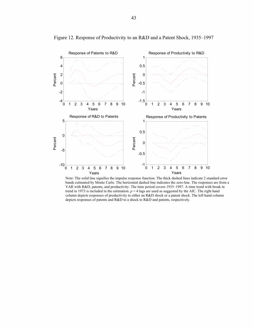
43

Figure 12. Response of Productivity to an R&D and a Patent Shock, 1935–1997

0 1 2 3 4 5 6 7 8 9 10-4

-2

0

2

4

6Response of Patents to R&D

Per

cent

Years0 1 2 3 4 5 6 7 8 9 10

-1.5

-1

-0.5

0

0.5

1Response of Productivity to R&D

Per

cent

Years

0 1 2 3 4 5 6 7 8 9 10-10

-5

0

5Response of R&D to Patents

Per

cent

Years0 1 2 3 4 5 6 7 8 9 10

-1

-0.5

0

0.5

1Response of Productivity to Patents

Per

cent

Years Note: The solid line signifies the impulse response function. The thick dashed lines indicate 2 standard error bands estimated by Monte Carlo. The horizontal dashed line indicates the zero-line. The responses are from a VAR with R&D, patents, and productivity. The time period covers 1935–1997. A time trend with break in trend in 1973 is included in the estimation. p = 4 lags are used as suggested by the AIC. The right hand column depicts responses of productivity to either an R&D shock or a patent shock. The left hand column depicts responses of patents and R&D to a shock to R&D and patents, respectively.

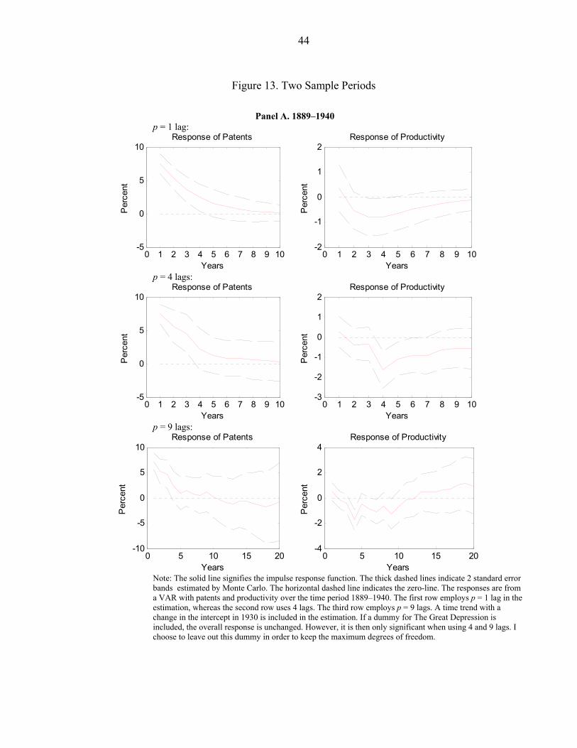
44

Figure 13. Two Sample Periods

Panel A. 1889–1940

p = 1 lag:

0 1 2 3 4 5 6 7 8 9 10-5

0

5

10Response of Patents

Per

cent

Years0 1 2 3 4 5 6 7 8 9 10

-2

-1

0

1

2Response of Productivity

Per

cent

Years p = 4 lags:

0 1 2 3 4 5 6 7 8 9 10-5

0

5

10Response of Patents

Per

cent

Years0 1 2 3 4 5 6 7 8 9 10

-3

-2

-1

0

1

2Response of Productivity

Per

cent

Years p = 9 lags:

0 5 10 15 20-10

-5

0

5

10Response of Patents

Per

cent

Years0 5 10 15 20

-4

-2

0

2

4Response of Productivity

Per

cent

Years Note: The solid line signifies the impulse response function. The thick dashed lines indicate 2 standard error bands estimated by Monte Carlo. The horizontal dashed line indicates the zero-line. The responses are from a VAR with patents and productivity over the time period 1889–1940. The first row employs p = 1 lag in the estimation, whereas the second row uses 4 lags. The third row employs p = 9 lags. A time trend with a change in the intercept in 1930 is included in the estimation. If a dummy for The Great Depression is included, the overall response is unchanged. However, it is then only significant when using 4 and 9 lags. I choose to leave out this dummy in order to keep the maximum degrees of freedom.

45

Panel B. 1948–2002 p = 1 lag:

0 1 2 3 4 5 6 7 8 9 10-2

0

2

4

6

8Response of Patents

Per

cent

Years0 1 2 3 4 5 6 7 8 9 10

-0.5

0

0.5

1

1.5Response of Productivity

Per

cent

Years

p = 4 lags:

0 1 2 3 4 5 6 7 8 9 10-2

0

2

4

6Response of Patents

Per

cent

Years0 1 2 3 4 5 6 7 8 9 10

-0.5

0

0.5

1Response of Productivity

Per

cent

Years

Note: The solid line signifies the impulse response function. The thick dashed lines indicate 2 standard error bands estimated by Monte Carlo. The horizontal dashed line indicates the zero-line. The responses are from a VAR with patents and productivity over the time period 1948–2002. The first row employs p = 1 lag in the estimation whereas the second row uses 4 lags. A time trend with a break in trend in 1973 is included in the estimation.

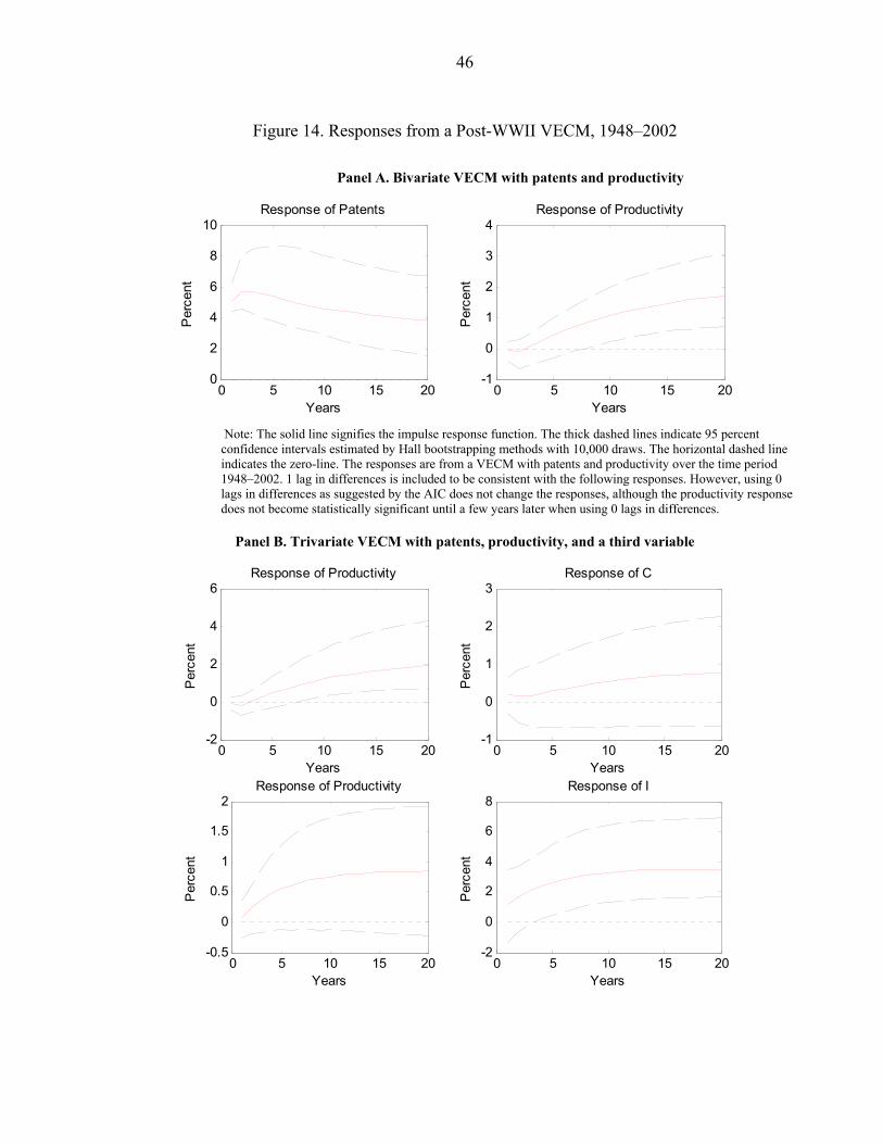
46

Figure 14. Responses from a Post-WWII VECM, 1948–2002

Panel A. Bivariate VECM with patents and productivity

0 5 10 15 200

2

4

6

8

10Response of Patents

Per

cent

Years0 5 10 15 20

-1

0

1

2

3

4Response of Productivity

Per

cent

Years

Note: The solid line signifies the impulse response function. The thick dashed lines indicate 95 percent confidence intervals estimated by Hall bootstrapping methods with 10,000 draws. The horizontal dashed line indicates the zero-line. The responses are from a VECM with patents and productivity over the time period 1948–2002. 1 lag in differences is included to be consistent with the following responses. However, using 0 lags in differences as suggested by the AIC does not change the responses, although the productivity response does not become statistically significant until a few years later when using 0 lags in differences.

Panel B. Trivariate VECM with patents, productivity, and a third variable

0 5 10 15 20-2

0

2

4

6Response of Productivity

Per

cent

Years0 5 10 15 20

-1

0

1

2

3Response of C

Per

cent

Years

0 5 10 15 20-0.5

0

0.5

1

1.5

2Response of Productivity

Per

cent

Years0 5 10 15 20

-2

0

2

4

6

8Response of I

Per

cent

Years

47

0 5 10 15 20-2

0

2

4

6Response of Productivity

Per

cent

Years0 5 10 15 20

-2

0

2

4Response of Y

Per

cent

Years

0 5 10 15 20-2

0

2

4

6Response of Productivity

Per

cent

Years0 5 10 15 20

-4

-3

-2

-1

0

1Response of H

Per

cent

Years Note: The solid line signifies the impulse response function. The thick dashed lines indicate 95 percent confidence intervals estimated by Hall bootstrapping methods with 5,000 draws. The horizontal dashed line indicates the zero-line. The responses are from a VECM with patents, productivity, and a third variable, depending on the measure of interest. The time period is 1948–2002. For consumption, C, 1 lag in differences is used as suggested by the AIC. For investment, I, 0 lags in differences are used as suggested by the AIC. For both output, Y, and hours, H, 1 lag in differences is used as suggested by the AIC.

Figure 15. Responses from a Post-WWII VAR, 1948–2002

Panel A. Bivariate VAR with patents and productivity

0 5 10 15 200

5

10

15

20Response of Patents

Per

cent

Years0 5 10 15 20

-2

0

2

4

6Response of Productivity

Per

cent

Years Note: The solid line signifies the impulse response function. The thick dashed lines indicate 95 percent confidence intervals estimated by Hall bootstrapping methods with 5,000 draws. The horizontal dashed line indicates the zero-line. The responses are from a VAR with patents and productivity over the time period 1948–2002. No deterministic trend included in the estimation. 2 lags are used to be consistent with the corresponding VECM above. Using 1 lag as suggested by the AIC does not change the responses.

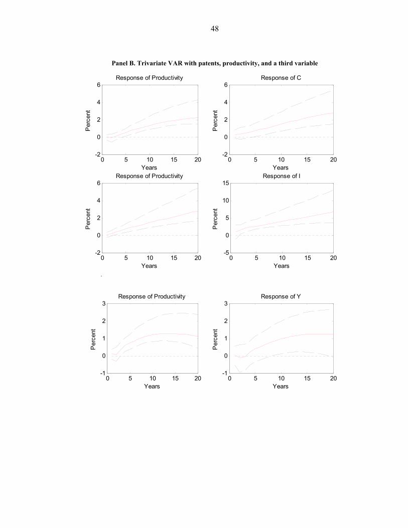
48

Panel B. Trivariate VAR with patents, productivity, and a third variable

0 5 10 15 20-2

0

2

4

6Response of Productivity

Per

cent

Years0 5 10 15 20

-2

0

2

4

6Response of C

Per

cent

Years

0 5 10 15 20-2

0

2

4

6Response of Productivity

Per

cent

Years0 5 10 15 20

-5

0

5

10

15Response of I

Per

cent

Years .

0 5 10 15 20-1

0

1

2

3Response of Productivity

Per

cent

Years0 5 10 15 20

-1

0

1

2

3Response of Y

Per

cent

Years

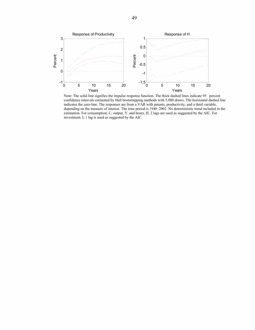
49

0 5 10 15 20-1

0

1

2

3Response of Productivity

Per

cent

Years0 5 10 15 20

-1.5

-1

-0.5

0

0.5

1Response of H

Per

cent

Years Note: The solid line signifies the impulse response function. The thick dashed lines indicate 95 percent confidence intervals estimated by Hall bootstrapping methods with 5,000 draws. The horizontal dashed line indicates the zero-line. The responses are from a VAR with patents, productivity, and a third variable, depending on the measure of interest. The time period is 1948–2002. No deterministic trend included in the estimation. For consumption, C, output, Y, and hours, H, 2 lags are used as suggested by the AIC. For investment, I, 1 lag is used as suggested by the AIC.

50

APPENDIX I

Patent Data Patent data are total annual utility patent applications received by the U.S. Patent and Trademark Office for the period 1889 – 2002. Patents granted are from the same source.

Labor productivity, hours, and output in private business

Data for labor productivity (Output per Manhour), real output, and hours are from Kendrick (1961) table A-XXII and table A-X for the period 1889 – 1946 and from the Bureau of Labor Statistics (BLS) for the period 1947–2002. The series are spliced by multiplying the pre-1947 data by the ratio of the BLS data in 1947 to the Kendrick data in 1947.

Real GDP, Consumption, Investment Real GNP is from Balke and Gordon (1989) for the period 1889–1928. Real consumption expenditures and gross private investment are from Kendrick (1961), Table A-IIa for the period 1889–1928. Nominal consumption and GNP are from Kendrick (1961), Table A-IIb for the period 1889–1928. For the period 1929–2002, nominal GDP, chain-weighted GDP, consumption, and investment are from Bureau of Economic Analysis (BEA), NIPA data. The series were spliced in 1929 by multiplying pre-1929 data with the ratio of the NIPA data in 1929 to Kendrick’s data in 1929.

Income and Wage inequality The top decile and other fractiles for the income share, 1917–1998, and the top decile and other fractiles for the wage share, 1927–1998, are from Piketty and Saez (2003).

R&D R&D for 1935–1997 is investment in privately financed research and development, deflated by chain-type price index for GDP and as computed by NPA Data Services. The data are available in Terleckyj, Levy, and Coleman (1997).

Diffusion of products Data on spread of products into American households, 1900–2004, are provided by W. Michael Cox, Federal Reserve Bank of Dallas. Data on diffusion of electric power are from Du Boff (1979).

Stock price index Data on stock prices are real S&P Composite Stock Price Index 1889–2002. Data are available at a monthly frequency on http://www.econ.yale.edu/~shiller/data.htm. This site contains updated data for chapter 26 of Market Volatility, Shiller (1989), and Irrational Exuberance, Shiller (2005). The January annualized values are the values used by Shiller in Market Volatility, chapter 26 and updated by Shiller while the June values are taken directly from the monthly data as computed by Shiller.

51

REFERENCES

Alexopoulos, Michelle, 2006, “Read all about it!! What Happens Following a Technology

Shock?” Working Paper, University of Toronto. Alm, Richard, and W. Michael Cox, 1996, “The Economy at Light Speed. Technology and

Growth in the Information Age and Beyond,” Federal Reserve Bank of Dallas, Annual Report.

Balke, Nathan S., and Robert J. Gordon, 1989, “The Estimation of Prewar Gross National

Product: Methodology and New Evidence,” Journal of Political Economy, Vol. 97, No. 1, pp. 38–92.

Bartel, Ann P., 1989, “Formal Employee Training Programs and Their Impact on Labor Productivity: Evidence from a Human Resources Survey,” NBER Working Paper No. 3026 (Cambridge, Massachusetts: National Bureau of Economic Research).

———, and Nachum Sicherman, 1999, “Technological Change and Wages: An Interindustry

Analysis,” Journal of Political Economy, Vol. 107, No. 2, pp. 285–325. Basu, Susanto, John G. Fernald, and Miles S. Kimball, 2006, “Are Technology Improvements

Contractionary?” American Economic Review, Vol. 96, No. 5, pp. 1418–48. Beaudry, Paul, and Franck Portier, 2006, “Stock Prices, News and Economic Fluctuations,”

American Economic Review, Vol. 96, No. 4, pp. 1293–1307.

Bhansali, R. J., 1997, “Direct Autoregressive Predictors for Multistep Prediction: Order Selection and Performance Relative to the Plug in Predictors,” Statistica Sinica,

Vol. 7, pp. 425–49. Comin, Diego, and Bart Hobijn, 2004, “Cross-Country Technology Adoption: Making the

Theories Face the Facts,” Journal of Monetary Economics, Vol. 51, No. 1, pp. 39–83. David, Paul A., 1990, “The Dynamo and the Computer: An Historical Perspective on the

Modern Productivity Paradox,” American Economic Review, Vol. 80, No. 2, Papers and Proceedings of the Hundred and Second Annual Meeting of the American Economic Association, pp. 355–61.

Devine, Warren D., Jr., 1983, “From Shafts to Wires: Historical Perspective on Electrification,”

Journal of Economic History, Vol. 43, No. 2, pp. 347–72. Du Boff, and Richard B., 1979, Electrical Power in American Manufacturing, 1889–1958

(Arno Press: New York).

52 Francis, Neville, and Valerie A. Ramey, 2004, “The Source of Historical Economic

Fluctuations: An Analysis using Long-Run Restrictions,” BEA Working Paper No. 10631 (Washington, D.C.: Bureau of Economic Analysis).

Gali, Jordi, 1999, “Technology, Employment, and the Business Cycle: Do Technology Shocks

Explain Aggregate Fluctuations?” American Economic Review, Vol. 89, No. 1, pp. 249–71. Greenwood, Jeremy, and Mehmet Yorukoglu, 1997, “1974,” Carnegie-Rochester Conference

Series on Public Policy, Vol. 46, pp. 49–95. Griliches, Zvi, 1990, “Patent Statistics as Economic Indicators: A Survey,” Journal of

Economic Literature, Vol. 28, No. 4, pp. 1661–1707.

Hall, Bronwyn, 2004 ,“Innovation and Diffusion,” NBER Working Paper No. 10212, (Cambridge, Massachusetts: National Bureau of Economic Research).

———, Adam B. Jaffe, and Manuel Trajtenberg, 2001, “The NBER Patent Citations Data File: Lessons, Insights, and Methodological Tools”, NBER Working Paper No. 8498 (Cambridge, Massachusetts: National Bureau of Economic Research).

Hall, Bronwyn H., and Manuel Trajtenberg, 2004, “Uncovering GPTs With Patent Data,”

NBER Working Paper No. 10901 (Cambridge, Massachusetts: National Bureau of Economic Research).

Hamilton, James D., 1994, Time Series Analysis (Princeton, New Jersey: Princeton University

Press). Hornstein, Andreas, and Per Krusell, 1996, “Can Technology Improvements Cause Productivity

Slowdowns?” NBER Macroeconomics Annual 1996, ed. by Ben S. Bernanke and Julio J. Rotemberg, pp. 209–59 (Cambridge, Massachusetts: National Bureau of Economic Research).

Jovanovic, Boyan, and Peter L. Rousseau, 2005, “General Purpose Technologies,” NBER

Working Paper No. 11093 (Cambridge, Massachusetts: National Bureau of Economic Research).

Kendrick, John W., 1961, “Productivity Trends in the United States,” NBER Working Paper

No. 71 (National Bureau of Economic Research, General Series, Princeton University Press).

Kortum, Samuel, and Josh Lerner, 1998, “Stronger Protection or Technological Revolution:

What is Behind the Recent Surge in Patenting?” Carnegie-Rochester Conference Series on Public Policy, Vol. 4. pp. 247–304.

53 Krusell, Per, and Lee E. Ohanian, Jose-Victor Rios-Rull, and Giovanni L. Violante, 2000,

“Capital-Skill Complementarity and Inequality: A Macroeconomic Analysis,” Econometrica, Vol. 68, No. 5, pp. 1029–53.

Lach, Saul, 1995, “Patents and Productivity Growth at the Industry Level: A First Look,”

Economics Letters, Vol. 49, pp. 101–08. ———, and Mark Schankerman, 1989, “Dynamics of R&D and Investment in the Scientific

Sector,” Journal of Political Economy, Vol. 97, No. 4, pp. 880–904. Mensch, Gerhard, 1975, Stalemate in Technology: Innovations Overcome the Depression

(Cambridge, Massachusetts: Ballinger Publishing Company). National Academy of Engineering. Greatest Achievements. Available via the Internet:

http://www.greatachievements.org/greatachievements/index.html. Nordhaus, William, 2005, “The Sources of the Productivity Rebound and the Manufacturing

Employment Puzzle,” NBER Working Paper No. 11354 (Cambridge, Massachusetts: National Bureau of Economic Research).

Perron, Pierre, 1989,“The Great Crash, the Oil Price Shock, and the Unit Root Hypothesis,”

Econometrica, Vol. 57, No. 6, pp. 1361–1401.

Piketty, Thomas, and Emmanuel Saez, 2003, “Income Inequality in the United States, 1913–98,” Quarterly Journal of Economics, Vol. 118, No. 1.

Ramey, Valerie A., 2006 ,“Identifying Government Spending Shocks: It’s All in the Timing,” Available via the Internet: http://www.econ.ucsd.edu/%7Evramey/research.html.

———, and Matthew D. Shapiro, 1998, “Costly Capital Reallocation and the Effects of

Government Spending,” Carnegie-Rochester Conference Series on Public Policy, Vol. 48, pp. 145–94.

Rogers, Everett M., 1995, Diffusion of Innovations (New York: Free Press, 4th ed.). Rotemberg, Julio J., 2003, “Stochastic Technical Progress, Smooth Trends, and Nearly Distinct

Business Cycles,” American Economic Review, Vol. 93, No. 5, pp. 1543–59. Schmookler, Jacob, 1972, “Patents, Invention, and Economic Change: Data and Selected

Essays,” ed. by Zvi Griliches and Leonid Hurwicz (Cambridge, Massachusetts: Harvard University Press).

Shea, John, 1998, “What do Technology Shocks Do?” NBER Macroeconomics Annual, ed. by Ben S. Bernanke and Julio J. Rotemberg, pp. 275–310.

54 Shiller, Robert J., 1989, “Market Volatility”, The MIT Press, Cambridge, Massachusetts. ———, 2000, Irrational Exuberance (Princeton, New Jersey: Princeton University Press,

updated 2005).

Solow, Robert M., 1987, “We’d Better Watch Out,” Book Review in the New York Times, pp. 36. Sullivan, Richard J., 1990, “The Revolution of Ideas: Widespread Patenting and Invention

During the English Industrial Revolution,” Journal of Economic History, Vol. 50, No. 2, pp. 349–62.

Terleckyj, Nestor E., David M. Levy, and Charles D. Coleman, 1997, “Model of U.S. Economic

Growth (Version 97.O): Technical Description, Model Software and Database. Special Issue,” National Economic Projections Series, Vol. 3, Report Number 97-N-3, NPA Data Services, Inc, Washington, DC.

Trajtenberg, Manuel, 2001 ,“Innovation in Israel 1968–97: A Comparative Analysis Using Patent Data,” Research Policy, Vol. 30, pp. 363–89.