changing business dynamism and productivity: shocks versus
TRANSCRIPT
American Economic Review 2020, 110(12): 3952–3990 https://doi.org/10.1257/aer.20190680
3952
* Decker: Federal Reserve Board (email: [email protected]); Haltiwanger: University of Maryland andNBER (email: [email protected]); Jarmin: US Census Bureau (email: [email protected]); Miranda: US Census Bureau (email: [email protected]). John Haltiwanger is also a Schedule A part-time employee of the USCensus Bureau at the time of the writing of this paper. Emi Nakamura was the coeditor for this article. We grate-fully acknowledge financial support from the Kauffman Foundation. Cody Tuttle provided excellent research assistance. We thank John Abowd, Rudi Bachmann, Martin Baily, Jonathan Baker, Dave Byrne, Chris Foote, Lucia Foster, Clément Gorin, Bronwyn Hall, Matthias Kehrig, Pete Klenow, Kristin McCue, three anonymous referees, and conference or seminar participants at the 2015 Atlanta Fed Conference on Secular Changes in Labor Markets, the ASSA 2016 meetings, the 2016 Brookings “productivity puzzle” conference, the 3rd International ZEW conference, the 2016 ICC conference, BYU, University of Chicago, Drexel University, the Federal Reserve Board, the Richmond Fed, the spring 2017 Midwest Macro meetings, the 2017 UNC IDEA conference, and the 2017 NBER Summer Institute meetings for helpful comments. We are grateful for the use of the manufacturing productivity database developed in Foster, Grim, and Haltiwanger (2016) as well as the revenue productivitydatabase developed in Haltiwanger et al. (2017). Any opinions and conclusions expressed herein are those of theauthors and do not necessarily represent the views of the US Census Bureau or of the Board of Governors or its staff. The statistics reported in this paper have been reviewed and approved by the Disclosure Review Board of the Bureau of the Census ( DRB-B0029-CED-20190314, DRB-B0056-CED-20190529, CBDRB-FY20-138).
† Go to https://doi.org/10.1257/aer.20190680 to visit the article page for additional materials and author disclosure statements.
Changing Business Dynamism and Productivity: Shocks versus Responsiveness†
By Ryan A. Decker, John Haltiwanger, Ron S. Jarmin, and Javier Miranda*
The pace of job reallocation has declined in the United States in recent decades. We draw insight from canonical models of business dynamics in which reallocation can decline due to (i ) lower dis-persion of idiosyncratic shocks faced by businesses, or (ii ) weaker marginal responsiveness of businesses to shocks. We show that shock dispersion has actually risen, while the responsiveness of business-level employment to productivity has weakened. Moreover, declining responsiveness can account for a significant fraction of the decline in the pace of job reallocation, and we find suggestive evidence this has been a drag on aggregate productivity. (JEL D24, E24, E32, J21, J23, J24, L60)
Changing patterns of business dynamics, i.e., the entry, growth, decline, and exit of businesses, have attracted increasing attention in recent literature. In par-ticular, since the early 1980s the United States has seen a decline in the pace of “business dynamism” across many measures including the rate of business entry, the prevalence of high-growth firm outcomes, the rate of internal migration, and the rate of job and worker reallocation.1 Declining business dynamism has
1 For job reallocation and employment volatility, see Davis et al. (2007) and Decker et al. (2014, 2016b). Forbusiness entry, see Decker et al. (2014) and Karahan, Pugsley, and Sahin (2018). For worker reallocation, see Hyatt and Spletzer (2013) and Davis and Haltiwanger (2014). For migration, see Molloy et al. (2016). For high-growthfirms, see Decker et al. (2016b); Haltiwanger, Hathaway, and Miranda (2014); and Guzman and Stern (2016).
3953DECKER ET AL.: CHANGING BUSINESS DYNAMISM AND PRODUCTIVITYVOL. 110 NO. 12
attracted attention in part because business dynamics are closely related to aggre-gate productivity growth in healthy market economies, reflecting the movement of resources from less-productive to more-productive uses (Hopenhayn and Rogerson 1993; Foster, Haltiwanger, and Krizan 2001). We draw insights from canonical models of firm dynamics in which declining reallocation reflects either a decline in the responsiveness of individual businesses to their underlying productivity or a decline in the dispersion of firm-level productivity shocks. Empirically, we find robust evidence of declining firm-level responsiveness amid rising dispersion of firm-level productivity shocks. We show that declining responsiveness accounts for a significant share of the aggregate decline in job reallocation and has been a drag on aggregate productivity.
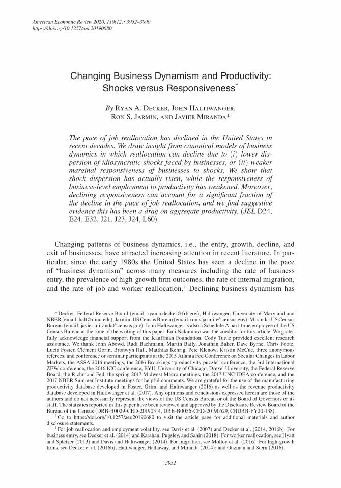
“Job reallocation” measures the pace of job flows across businesses and is defined as total job creation by entering and expanding establishments plus total job destruc-tion by downsizing and exiting establishments. Figure 1 shows the pace of aggre-gate job reallocation for the United States overall, the manufacturing sector, and the high-tech sector. The United States experienced an overall decline in the pace of job reallocation since the early 1980s. Even the high-tech sector saw a decline starting in the early 2000s. Understanding the causes of declining job reallocation has proven difficult. Decker et al. (2016b) show that it reflects in part a decline in firm-level growth rate skewness, or high-growth firm activity generally, but they do not investigate underlying causes. Young firms tend to exhibit a higher pace of job reallocation, and the share of activity accounted for by young firms has declined (Decker et al. 2014), so some decline in reallocation is to be expected given compo-sition effects. However, most of the variation in reallocation rates in recent decades has occurred within narrow age classes.2
2 In online Appendix Section III we describe a shift-share exercise to study the role of composition effects across firm age for explaining the overall decline in job reallocation. Online Appendix Figure A5 reports the results. We are sympathetic to the view that studying the sources of the decline in startups and young firms is important for understanding the decline in job reallocation (e.g., Pugsley, Sedlácek, and Sterk 2017). Our focus is on the decline in job reallocation within firm age groups, which Figure A5 shows is quite important.
Figure 1. Job Reallocation Patterns Differ by Sector
Notes: HP trends using parameter set to 100. Industries defined on a consistent NAICS basis; high-tech is defined as in Hecker (2005). Data include all firms (new entrants, continuers, and exiters).
Source: LBD
15
20
25
30
35
Per
cent
of e
mpl
oym
ent
1981
1983
1985
1987
1989
1991
1993
1995
1997
1999
2001
2003
2005
2007
2009
2011
2013
Economywide High-techManufacturing High-tech manufacturing

3954 THE AMERICAN ECONOMIC REVIEW DECEMBER 2020
We study changing job reallocation patterns motivated by the framework of stan-dard models of firm dynamics following Hopenhayn (1992) and a rich subsequent literature. In such models, reallocation arises from businesses’ responses to their constantly shifting individual productivity and profitability environment. Businesses facing strong idiosyncratic productivity and profitability conditions expand (job creation), while those facing weak conditions downsize or exit (job destruction). The reallocation rate reflects the aggregation of these individual decisions. As such, a decline in the pace of reallocation can arise from one of two forces. First, the dispersion or volatility of idiosyncratic ( business-level) conditions (which we call “shocks”) could decline; in other words, a more tranquil business environment could reduce the need and incentives for businesses frequently and significantly to change their size or operating status. Second, or alternatively, the business-level responsive-ness to those shocks could weaken; that is, businesses may hire or downsize less in response to a given shock (conditional on their initial level of employment), perhaps due (for example) to rising costs of factor adjustment.
These model-based considerations give rise to two competing hypotheses for declining job reallocation rates: the “shocks” hypothesis, in which the dispersion of idiosyncratic productivity or profitability realizations has declined; and the “respon-siveness” hypothesis, in which businesses have become more sluggish in responding to realized shocks.3 We explore these hypotheses in high-quality business microdata for the United States. We show that the dispersion of “shocks” faced by individual businesses has not in fact declined but has risen. However, business-level respon-siveness to those shocks has declined markedly in the manufacturing sector and in the broader US economy.4
These changes in responsiveness largely account for the observed decline in aggregate job reallocation. In the manufacturing sector, where we have high-quality measures of establishment-level productivity, we find that declining responsiveness accounts for virtually all of the decline in the pace of job reallocation from the 1980s to the post-2000 period (holding constant the age distribution of businesses). Even outside of manufacturing, where we have a more limited measure of firm-level pro-ductivity, declining responsiveness can account for about half of the late-1990s to post-2010s decline in job reallocation.
Business-level responses to productivity also facilitate productivity selection, and weaker responsiveness is indicative of weaker selection. We isolate the effect of changing responsiveness on an index of aggregate productivity using a simple coun-terfactual exercise. Aggregate total factor productivity (TFP) increased by about 30 percent in the US manufacturing sector from the 1980s to 2000s, but our counter-factual exercise suggests TFP would have increased by about 33 percent if respon-siveness in the 2000s were the same as in the early 1980s. We find similar effects on aggregate labor productivity for the US private, nonfarm sector.
3 The general “shocks versus responsiveness” framework has proven useful elsewhere: see Berger and Vavra (2019).
4 Rising labor productivity dispersion outside manufacturing was first documented in a related working paper (Decker et al. 2016a) and in Barth et al. (2016). Andrews, Criscuolo, and Gal (2015) documented rising gaps in the growth of firm-level labor productivity in several OECD countries. Kehrig and Vincent (2017, 2020) present related evidence of a decline in responsiveness to a shock concept we denote as TFPR in our analysis below.

3955DECKER ET AL.: CHANGING BUSINESS DYNAMISM AND PRODUCTIVITYVOL. 110 NO. 12
Taken together, our results suggest that declining reallocation is not simply a benign result of a less turbulent economy. Rather, declining reallocation appears to reflect weaker responses of businesses to their own economic environment, and the consequences of weaker responsiveness for aggregate living standards are nontriv-ial due to the important role of productivity selection. Determining the causes of weakening responsiveness is beyond the scope of this paper; however, we describe several possible avenues of investigation that are suggested by the model framework we employ.
Section I describes our conceptual framework and its empirical predictions for the “shocks” and “responsiveness” hypotheses. Section II describes our data, includ-ing our measures of productivity. Section III describes our empirical approach and results on “shocks” and “responsiveness.” Section IV quantifies the implications for aggregate reallocation and productivity. Section V describes robustness exercises, and Section VI concludes.
I. Conceptual Framework
A. General Formulation
We begin by specifying, in quite general terms, the relationship of firm-level employment growth to firm-level productivity realizations (shocks) and initial employment in a one-factor (labor) model of business dynamics.5 Consider the employment growth policy function given by
(1) g jt = f t ( A jt , E jt−1 ) ,
where g jt is employment growth for firm j from t − 1 to t , A jt is the productivity (or, more generally, profitability) realization in time t , and E jt−1 is initial employ-ment. More concretely, we can motivate the canonical formulation in (1) with a model in which firms have a revenue function given by A jt E jt
ϕ , where ϕ < 1 due to either decreasing returns or imperfect competition; and the productivity process is ln A jt = ρ a ln A jt−1 + η jt (so η jt is the innovation to productivity in period t ). In typ-ical models of this nature, ∂ f / ∂ A > 0 ; that is, among any two firms, the one with higher A jt , holding initial employment constant, will have higher growth. We also include a time subscript t in f t ( ∙ ) to allow the relationship between growth and the underlying state variables to change over time (due, e.g., to changing employment adjustment costs).
While some expositions of this class of models specify g jt as a function of the change in productivity (or of the innovation η jt ), we deliberately feature the level of A jt in (1). Empirically, it is easier to relate the growth rate of firms (for which we have universe data) to productivity levels (for which we have cross-sectionally rep-resentative samples) than to changes or innovations (which require productivity data that are longitudinally representative). Moreover, the formulation in which A jt is specified in levels, as in (1), is quite general since, under minimal assumptions, the
5 We use the term “firm” loosely in this section. Our empirics feature both firm- and establishment-level data.

3956 THE AMERICAN ECONOMIC REVIEW DECEMBER 2020
inclusion of E jt−1 along with A jt in the policy function fully incorporates information contained in A jt−1 and, therefore, the difference between A jt and A jt−1 .6 That is, we can specify (1) using the level of A jt and initial employment without significant loss of generality while improving the model’s empirical comparability.
For empirical purposes, we focus on a log-linear approximation of (1) given by
(2) g jt = β 0 + β 1t a jt + β 2t e jt−1 + ε jt ,
where the lowercase variables a and e refer to the logs of productivity and employ-ment, respectively. The parameter β 1t is our measure of productivity responsiveness: it measures the marginal response of firm employment growth to firm productiv-ity. In the typical model setting β 1t > 0 , but the magnitude of this relationship depends on model parameters, distortions, adjustment frictions, and potentially firm characteristics (as we describe below). We refer to a change in β 1t as a change in responsiveness. Since the policy function specified in (1) and approximated by (2) determines firm-level employment changes, it also determines the aggregate job reallocation rate (which is simply the employment-weighted average of the absolute value of firm-level growth). Therefore, a decline in reallocation can be caused by either a decline in marginal responsiveness ( β 1t ) or a change in the distribution of A jt shocks, a quite general result.
We next explore two concrete model specifications to illustrate numerically the implications of the shocks versus responsiveness hypotheses.
B. Labor Adjustment Costs
Consider a canonical model of firm dynamics with labor adjustment costs in the tradition of Hopenhayn and Rogerson (1993). For simplicity we abstract from firm entry and exit. Faced with costs on labor adjustment, firms no longer adjust their labor demand to reach the firm size that would be implied by A jt in a frictionless environment. Moreover, an increase in adjustment costs reduces responsiveness to A jt (conditional on initial employment).
In online Appendix Section I, we describe this model in detail under both non-convex cost and convex cost specifications; here, we initially summarize the results of numerical simulations using the model with non-convex adjustment costs (with the kinked adjustment costs explored in Hopenhayn and Rogerson 1993, Cooper, Haltiwanger, and Willis 2007, and Elsby and Michaels 2013). We then pro-vide an overview of the analogous results with convex adjustment costs. We solve the model then simulate a panel of firms, allowing us to study job reallocation and productivity responsiveness ( β 1t from equation (2)) as well as another key moment, the dispersion of revenue per worker. The results using non-convex adjustment costs are in Figure 2.
Panels A and B of Figure 2 illustrate our central hypotheses: declining realloca-tion can result from rising adjustment costs (i.e., lower responsiveness), as shown in
6 We formally show this in the online Appendix. The employment growth policy function can be specified in terms of levels of A jt even in a frictionless model. Nevertheless, our empirical exercises are all robust to specifying the growth policy function in terms of changes in, or innovations to, A jt .

3957DECKER ET AL.: CHANGING BUSINESS DYNAMISM AND PRODUCTIVITYVOL. 110 NO. 12
panel A, or from declining shock (TFP or a jt ) dispersion, as shown in panel B. Wefocus first on adjustment costs. As these costs rise, job reallocation falls (panel A)because the responsiveness coefficient weakens (the red long-dashed line on panelC). As a result, dispersion of revenue per worker rises (the short-dashed green linein panel C). In the absence of adjustment costs, equalization of marginal productswould imply zero dispersion of revenue per worker; with adjustment costs, rev-enue per worker is positively correlated with a jt and exhibits positive dispersion. Additionally, as we show in online Appendix Figure A4, aggregate productivity declines as adjustment costs rise.
Alternatively, declining reallocation can result from declining dispersion of a jt as shown in panel B of Figure 2. Panel D shows that, in this scenario, the disper-sion of revenue productivity falls, as does the responsiveness coefficient. Therefore, this model can generate a decline in job reallocation if a jt dispersion falls; other
Figure 2. The Shocks and Responsiveness Hypotheses, Model Results ( Non-Convex Cost)
Notes: Panels C and D share same legend. Results relative to model baseline calibration (vertical purple line)with downward adjustment cost F_ = 0 and TFP dispersion σA = 0.46 (see online Appendix Section I andTable A1 for model calibration details). SD RLP refers to the standard deviation of revenue labor productivity in model-simulated data.
Bas
elin
e ca
libra
tion
Bas
elin
eca
libra
tion
Bas
elin
eca
libra
tion
0.1.2
1
0
0.05
0.1
0.15
0.2
Rea
lloca
tion
rate
(sha
re o
f em
p.)
0 0.1 0.2 0.3 0.4 0.5
Downward adjustment cost F_
0 0.1 0.2 0.3 0.4 0.5
Downward adjustment cost F_
Panel A. Reallocation and adjustment costs
Bas
elin
e ca
libra
tion
0.1.2
1
0
0.05
0.1
0.15
0.2
Rea
lloca
tion
rate
(sha
re o
f em
p.)
0.3 0.35 0.4 0.45
TFP dispersion (σA)
Panel B. Reallocation and TFP dispersion
0.5
0.6
0.7
0.8
0.9
Responsiveness coefficient β
1
0.15
0.2
0.25
0.3
SD
RLP
Std. dev. of labor prod. (left)Responsiveness coeff. β1 (right)
Panel C. Effects of rising adjustment costs
0.15
0.2
0.25
0.3
SD
RLP
Panel D. Effects of changing TFP dispersion
0.3 0.35 0.4 0.45
TFP dispersion (σA)
0.5
0.6
0.7
0.8
0.9
Responsiveness coefficient β
1

3958 THE AMERICAN ECONOMIC REVIEW DECEMBER 2020
symptoms of declining a jt dispersion are weaker responsiveness and lower revenue productivity dispersion.
All results in Figure 2 also hold under convex adjustment costs except for the dependence of the responsiveness coefficient on the dispersion of a jt (see online Appendix discussion and Figure A1).7 Under convex adjustment costs, decision rules are approximately linear (see, e.g., Caballero, Engel, and Haltiwanger 1997), such that changes in second moments of shocks do not affect marginal responsive-ness; responsiveness does not decline with a jt dispersion under convex adjustment costs.8 The non-convex case therefore introduces some interaction between the shocks and responsiveness hypotheses, which we discuss further below.
C. Correlated “Wedges”
The properties of the formulation in (1) and (2) are more general than the spe-cific adjustment cost specifications just described. For example, consider a model with revenue function given by S jt A jt E jt
ϕ , where S jt is a firm-specific distortion or “wedge” that can be thought of as a tax (when S jt < 1 ) or a subsidy (when S jt > 1 ). Let wedges be related to fundamentals, such that log wedges (lower case) are deter-mined by s jt = − κ a jt + ν jt where, consistent with much of the recent literature, we assume κ ∈ (0,1) , and v jt is independent of a jt with 피( v jt ) = 0 .9 In online Appendix Section I we show that an increase in κ acts in the same fashion as an increase in adjustment costs: reallocation declines, responsiveness declines, revenue labor productivity dispersion rises, and aggregate productivity declines (throughout the paper, we refer to increasing κ as “increasingly correlated wedges”). A decline in the dispersion of productivity shocks also yields a decline in reallocation and revenue productivity dispersion but, as in the convex adjustment cost model, respon-siveness is not sensitive to dispersion in a jt . The properties of the correlated wedge model are illustrated in online Appendix Figure A2.
This wedge specification could be viewed as a reduced form encompassing the adjustment cost specification discussed in Subsection IB (albeit with some import-ant subtle differences given the explicitly dynamic components of an adjustment cost model). But this interpretation also may capture other possible changes in the distribution of wedges. For example, rising dispersion in variable markups that are
7 For both the non-convex (Figure 2) and convex (online Appendix Figure A1) setups we arrange the baseline scenario to target the pace of job reallocation in the 1980s among continuing US manufacturing establishments; we also use the 1980s moments for the dispersion and persistence of shocks (see online Appendix Table A1). The qual-itative pattern of the impact of changing adjustment costs on responsiveness is similar across cost specifications, but the convex cost case generates a baseline responsiveness coefficient that is more quantitatively similar to our empir-ical results. While we do not generate structural estimates of adjustment costs in this paper, Cooper, Haltiwanger, and Willis (2007) find that both convex and non-convex costs are needed to match the patterns in the data.
8 Non-convex adjustment costs give rise to inaction ranges. As productivity dispersion falls there is a decrease in the fraction of firms that make zero adjustment (i.e., the “real options” effect). But declining productivity dispersion also implies smaller adjustments among those firms that do adjust (i.e., the “volatility” effect). Vavra (2014) argues that the volatility effect dominates the real options effect in the steady state, a general result extending back to Barro (1972). Bloom (2009), Bloom et al. (2018), and others use a similar model to study the effects of uncertainty on business cycles; even in their model, the volatility effect dominates at annual frequency (see also Bachmann and Bayer 2013).
9 A common finding in the literature is that indirect measures of wedges (i.e., revenue productivity measures like TFPR) are positively correlated with measures of fundamentals (technical efficiency and demand shocks) and have lower variance than fundamentals: see Foster, Haltiwanger, and Syverson (2008), Hsieh and Klenow (2009), and Blackwood et al. (forthcoming).
3959DECKER ET AL.: CHANGING BUSINESS DYNAMISM AND PRODUCTIVITYVOL. 110 NO. 12
correlated with fundamentals can play a similar role (see, e.g., De Loecker, Eeckhout, and Unger 2020; Edmond, Midrigan, and Xu 2018; Autor et al. forthcoming).
D. Additional Considerations
Our discussion thus far has focused on the intensive margin of responsiveness. However, related predictions apply for the extensive margin: Hopenhayn and Rogerson (1993) find that a rise in adjustment frictions reduces entry and exit. The empirical prediction of increased adjustment costs, then, is that not only will the growth of continuing firms become less responsive to firm productivity, but so will exit, a prediction we explore empirically.
Our motivating discussion also neglects post-entry dynamics from learning that can influence the responsiveness of both the extensive and intensive margins by firm age (see, e.g., Jovanovic 1982). We consider this possibility in our empirical anal-ysis. This variation by firm age is interesting in its own right but also permits us to abstract from changes in average responsiveness due to the changing age structure of firms. Given the decline in the US firm entry rate in recent decades, if young firms have different average responsiveness from mature firms, aggregate responsiveness could have changed due to composition effects. We control for potentially exoge-nous changes in entry rates in the United States by studying responsiveness within firm age groups.
We consider additional nuances in our empirical work. For changes in the shock process, we consider not only the evolution of the dispersion in a jt but also, for restricted samples, the evolution of the dispersion of innovations to the shock pro-cess and the persistence of this process.10 We also estimate responsiveness to inno-vations or changes in productivity, and we explore how changes in responsiveness vary across industries that have undergone different trends in productivity disper-sion and persistence.
E. Summing Up
In general, reallocation declines when either responsiveness or shock ( a jt ) dis-persion decline. A decline in responsiveness can be generated by, for example, an increase in adjustment costs (convex or non-convex) or, more generally, an increase in the correlation between reduced form wedges and the a jt fundamental; in these cases, the dispersion of revenue labor productivity rises. A decline in the dispersion of the a jt shock, while capable of generating a decline in reallocation, also reduces the dispersion of revenue labor productivity (and, in the case of non-convex costs, reduces responsiveness as well). These model predictions provide sufficient empiri-cal moments for distinguishing between the shocks and responsiveness hypotheses. A critical point here is that we empirically examine both responsiveness and shock dispersion.
The gold standard empirical test of the responsiveness hypothesis is to estimate the changing relationship between the growth rate of employment and a jt , controlling for
10 In the adjustment cost framework, a decline in shock persistence can reduce responsiveness.

3960 THE AMERICAN ECONOMIC REVIEW DECEMBER 2020
initial employment. For the manufacturing sector, we can construct measures of a jt (and η jt , the innovation to a jt , for restricted samples). For other sectors, we can only measure revenue per worker. However, in the adjustment cost models, an increase in adjustment frictions also implies a declining covariance between growth and the realization of revenue per worker.11 Given this auxiliary prediction, we also explore changing “responsiveness” for non-manufacturing businesses using the changing relationship between employment growth and revenue per worker.
II. Data and Measurement
The main database for our analysis is the US Census Bureau’s Longitudinal Business Database (LBD), to which we attach other data as detailed below. The LBD includes annual location, employment, industry, and longitudinal linkages for the universe of private non-farm establishments, with firm identifiers based on oper-ational control (not an arbitrary tax identifier). Employment measures in the LBD come from payroll tax and survey data. We use the LBD for 1981–2013 (during which consistent establishment NAICS codes are available from Fort and Klimek 2016). For some exercises we focus on the high-tech sector; we define high-tech on a NAICS basis following Hecker (2005).12 As in previous literature, we construct firm age as the age of the firm’s oldest establishment when the firm identifier first appears in the data, after which the firm ages naturally.
For both our manufacturing and private sector economy analysis, we use the LBD to measure employment growth, initial employment, and exit (characterized as an establishment or firm that has positive employment activity in March of calendar year t and zero activity in March of calendar year t + 1 ). We use these LBD mea-sures of growth and exit even when we merge in productivity measures from else-where (described next); that is, we have measures of growth and exit for the universe of businesses.
A. Manufacturing: Measuring Establishment-Level Productivity
We construct establishment-level productivity for over 2 million plant-year observations ( 1981–2013) using updated data following the measurement meth-odology of Foster, Grim, and Haltiwanger (2016)—henceforth, FGH—combin-ing the Annual Survey of Manufacturers (ASM) with the quinquennial Census of Manufacturers (CM); see online Appendix Section II for detail. The resulting ASM-CM is representative of the manufacturing sector in any given year, but it is based on a rotating sample and thus lacks the complete longitudinal coverage of the LBD; this is why we use LBD measures of employment and employment growth.13
11 See online Appendix Figure A3a. These remarks also hold for revenue productivity measures such as TFPR as we discuss in our empirical analysis.
12 Hecker (2005) defines industries as high-tech based on the 14 four-digit NAICS industries with the largest share of STEM workers. This definition includes industries in manufacturing (NAICS 3254, 3341, 3342, 3344, 3345, 3364), information (5112, 5161, 5179, 5181, 5182), and services (5413, 5415, 5417).
13 We also use propensity score weights (based on a logit model of industry, firm size, and firm age) to adjust the ASM-CM-LBD sample to represent the LBD (in the cross section) in each year (see FGH). These weights are cross-sectionally representative in any given year but are not ideal for using samples of ASM-CM that are present in both t and t + 1 . We discuss this further below.

3961DECKER ET AL.: CHANGING BUSINESS DYNAMISM AND PRODUCTIVITYVOL. 110 NO. 12
Thus, a critical feature of our empirical approach (for manufacturing) is integrating the high-quality longitudinal growth measures from the LBD in any given year with the cross-sectional measures of productivity from the ASM-CM.
The productivity shocks we measure are intended to capture variation in both technical efficiency and demand or product appeal. To make our measurement approach transparent, it is helpful to be explicit about the assumed production and demand structure. Consider establishment-level demand function P jt = D jt Q jt
ϕ−1 (where D jt is an idiosyncratic demand shock, ϕ − 1 is the inverse demand elasticity, and j indexes establishments) with Cobb-Douglas production, that is, Q jt = A ̃ jt ∏ X jt
α x for inputs X jt (where A ̃ jt is technical efficiency, or TFPQ). A composite measure of productivity, “TFP,” reflecting idiosyncratic technical efficiency and demand shocks can be defined as A jt = D jt A ̃ jt
ϕ . The ASM-CM data provide survey-based measures of revenue, capital ( K ), employee hours ( L ), materials ( M ), and energy ( N ).14 Then establishment revenue is given by (lower case variables are in logs):
(3) p jt + q jt = β k k jt + β l l jt + β m m jt + β n n jt + ϕ a ̃ jt + d et ,
where β x = ϕ α x for factor X , and t denotes time (in years).15 The β x coefficients are factor revenue elasticities that reflect both demand parameters and production function factor elasticities. The implied revenue function residual, which we denote as TFP, is given by
(4) TFP jt = p jt + q jt − ( β k k jt + β l l jt + β m m jt + β n n jt ) = ϕ a ̃ jt + d jt ,
that is, this measure of TFP is a composite of idiosyncratic technical efficiency and demand shocks. In terms of the conceptual framework described previously (and in online Appendix Section I), this is the relevant measure of fundamental shocks consistent with demand and technology assumptions made in this section. With esti-mates of the revenue elasticities, this measure of TFP can be computed from observ-able establishment-level revenue and input data. We refer to this measure as TFP or “productivity” in what follows, but it should be viewed as the composite shock reflecting both technical efficiency and product demand or appeal. Our use of the revenue function residual to capture fundamentals is not novel to this paper. Cooper and Haltiwanger (2006) estimate the revenue function residual in their analysis of capital adjustment costs. Hsieh and Klenow (2009) use a closely related measure as
14 Labor input is total hours measured from the survey responses in the ASM/CM. We estimate factor elastici-ties for equipment and structures separately but refer only to generic “capital” for expositional simplicity here. See online Appendix Section II for more discussion of production factor measurement in the data.
15 Real revenue ( p + q ) is total value of shipments plus total change in the value of inventories, deflated by industry deflators from the NBER-CES Manufacturing Industry Database. Capital is measured separately for struc-tures and equipment using a perpetual inventory method. Labor is total hours of production and non-production workers. Materials are measured separately for physical materials and energy (each deflated by an industry-level deflator). Outputs and inputs are measured in constant 1997 dollars. More details are in online Appendix Section II.
3962 THE AMERICAN ECONOMIC REVIEW DECEMBER 2020
their empirical measure of TFPQ. 16 Blackwood et al. (forthcoming) use a similar measure in their analysis of allocative efficiency as a proxy for TFPQ.17
Below we discuss two alternative approaches to estimating the revenue function residual concept for TFP in (4), but first we describe another productivity concept that is widely used in the literature, TFPR, which is given by
(5) TFPR jt = p jt + q jt − ( α k k jt + α l l jt + α m m jt + α n n jt ) = p jt + a ̃ jt .
The key conceptual and measurement distinction between TFP in (4) and TFPR in (5) is using revenue versus output elasticities; under the assumptions made in this section, TFPR confounds technical efficiency and endogenous price factors. As emphasized by Foster, Haltiwanger, and Syverson (2008), Hsieh and Klenow (2009), and Blackwood et al. (forthcoming), this implies TFPR is an endoge-nous measure in this context (i.e., when prices are idiosyncratic and endogenous). Without frictions or wedges, TFPR will exhibit no within-industry dispersion and is therefore not an appropriate measure of fundamentals. With adjustment costs or correlated distortions, however, TFPR will be positively correlated with fundamen-tals. Empirically, TFPR and fundamentals are strongly positively correlated (Foster, Haltiwanger, and Syverson 2008 and Blackwood et al. forthcoming). The high cor-relation in practice helps rationalize the widespread use of TFPR as a measure of TFP in the empirical literature.18 For our purposes, TFPR is a useful measure since, in our model, an increase in adjustment costs, or increasingly correlated wedges, yield a decline in the responsiveness of growth to TFPR and a rise in dispersion of TFPR. In this respect, TFPR has properties similar to revenue per worker. We emphasize that, given the potential endogeneity limitation of TFPR, we do not con-sider it to be as clean a measure of “shocks” as is the TFP concept from (4). Rather, TFPR is a measure of revenue productivity (reflecting the product of prices and technical efficiency).
We now describe how we estimate our various manufacturing productivity measures. The construction of TFP from (4) requires estimates of the β x revenue elasticities. We obtain estimates in two different ways, resulting in two alternative TFP-based measures. Our first and preferred TFP measure relies on the first-order condition (for factor X ) from static profit maximization:
(6) α x ϕ = β x = W xt X jt _ P jt Q jt
,
16 The empirical measure of TFPQ used by Hsieh and Klenow (2009) is proportional to the rev-enue function residual measure of TFP given by (4). The measure they use for TFPQ (in logs) is ( p jt + q jt ) (1/ϕ) − ( α k k jt + α l l jt + α m m jt + α n n jt ) = a ̃ jt + ( d jt /ϕ) (see their equation (19)); that is, their TFPQ measure is equal to our measure of TFP from (4) divided by ϕ . While proportional, it is more challenging to construct their measure of TFPQ since it also requires an estimate of ϕ , which requires decomposing the revenue elasticities into their demand and output elasticities components (see Blackwood et al. forthcoming). Both the Hsieh and Klenow empirical measure and our measure are inclusive of any idiosyncratic demand shocks. Foster, Haltiwanger, and Syverson (2008) define TFPQ to be technical efficiency.
17 The gold standard is to use establishment- or firm-level prices permitting separation of technical efficiency and demand (and also alternative estimate approaches for output and demand elasticities). However, such prices are available for only limited products in the Economic Censuses (see Foster, Haltiwanger, and Syverson 2008).
18 It is also a measure of fundamentals if plants are price takers. Moreover, De Loecker et al. (2016) suggest that TFPR might be a preferred measure in the presence of unmeasured differences in materials prices and other inputs that reflect quality; output prices are likely correlated with such measures, so TFPR helps capture such variation.

3963DECKER ET AL.: CHANGING BUSINESS DYNAMISM AND PRODUCTIVITYVOL. 110 NO. 12
where W xt is the price of factor X , such that β x is the share of that factor’s costs in total revenue. The condition in (6) will not hold for all establishments at all times if there are adjustment frictions or wedges, but we only need (6) to hold on average when pooled through time and over establishments within industries, an assumption commonly used in the literature (e.g., Syverson 2011). We obtain factor shares of revenue from the NBER-CES database (at the 4-digit SIC level prior to 1997 and the 6-digit NAICS level thereafter) then extract revenue function residuals using equations (3) and (4). We call this measure TFPS (for “ TFP-Shares”).
Our second TFP measure is based on estimation of the revenue function in (3) using the proxy method GMM approach of Wooldridge (2009), allowing elasticities to vary at the 3-digit NAICS level (see online Appendix Section II for details; see other applications in, e.g., Gopinath et al. 2017 and Blackwood et al. forthcoming). We refer to this measure as TFPP (for “ TFP-Proxy”). The TFPP method allows us to avoid reliance on first-order conditions, but the estimation process involves high-order polynomials and so requires large samples. Following the literature, then, we use higher levels of aggregation for estimating industry elasticities: we use 3-digit NAICS compared to the 6-digit NAICS used for TFPS.19 This limitation of the proxy methods makes TFPS our preferred measure, but our results are robust to using TFPP.
For the TFPR measure from (5), we construct output elasticities as cost shares of inputs out of total costs (under the assumption of constant returns to scale).20 We use the NBER-CES productivity database to recover factor cost shares. Cost shares equal factor elasticities under the assumptions of cost minimization and full adjustment of factors; again, however, one need not assume full adjustment for each establishment in each time period but rather that this holds approximately when pooling across all plants in the same industry over time. Like TFPS, our TFPR mea-sure avoids the noisiness of estimation and allows us to use output elasticities that vary at the detailed industry level.
Our data are not ideally suited for tracking the persistence of, and innovations to, the TFP measures given the panel rotation of the ASM and our use of CM data. However, for results requiring us to estimate persistence of innovations, we exclude years for which we do not have a representative sample of continuing plants in t and t − 1 in our ASM-CM data (first panel years and Census years). Additionally, we acknowledge that our establishment-level measures of TFP are vulnerable to errors arising from omitted factors. For example, use of intangible capital in production is a potential source of measurement error (discussed further below).
Our preferred “shock” measures are TFPP and TFPS, which are measures of fun-damentals under the demand structure and production function assumptions made in this section. TFPR is a closely related measure but, under the same assumptions,
19 Blackwood et al. (forthcoming) find that the Wooldridge (2009) method residuals are highly sensitive to outliers, but pooling across more observations mitigates this problem.
20 See, e.g., Baily, Hulten, and Campbell (1992); Foster, Haltiwanger, and Krizan (2001); Syverson (2011); Ilut, Kehrig, and Schneider (2018); and Bloom et al. (2018). We construct time-invariant elasticities; in unreported exercises, we allow elasticities to vary over time with a Divisia index and find similar results.

3964 THE AMERICAN ECONOMIC REVIEW DECEMBER 2020
reflects both fundamentals and endogenous prices. Exploring richer demand and production structures is an open area for future research.21
B. Total Economy Revenue Labor Productivity
While TFP is the preferred concept in a shocks versus responsiveness framework, we can only estimate TFP in the manufacturing sector. For the economy generally, we rely on revenue per worker (“revenue labor productivity” or RLP), which is necessarily a firm-level (rather than establishment-level) concept in our data. As discussed above, rising adjustment frictions or increasingly correlated distortions also imply rising RLP dispersion and declining “responsiveness” of growth with respect to RLP.
Combining LBD employment (summed from the establishment to the firm level) with revenue measures in the Census Bureau’s Business Register (BR) (aggregated across EIN reporting units to the firm level) yields an enhanced LBD that we refer to as the RE-LBD.22 Revenue data are available from 1996 to 2013 and are derived from business tax returns.23 We construct annual firm employment growth rates on an “organic” basis to represent changes in establishment-level employment rather than artificial growth caused by mergers and acquisitions.24
For firm-level exercises, we assign each firm a consistent “modal” industry code based on the NAICS industry in which it has the most employment over time. In exercises reported in an earlier working paper version (Decker et al. 2018), we found our results are robust to an alternative approach in which we explicitly con-trol for all industries in which firms have activity rather than assigning each firm a single industry code. We omit firms in the Finance, Insurance, and Real Estate sectors (NAICS 52–53) from all analysis due to the difficulty of measuring output and productivity in those sectors.
21 Much attention has recently been given to the possibility of variable markups across producers in the same industry (e.g., De Loecker, Eeckhout, and Unger 2020). The De Loecker, Eeckhout, and Unger (2020) approach uses the cost shares of fully flexible production factors in total revenue to indirectly identify markups as a residual. An alternative approach to identification of variable markups is to maintain the CES demand structure assump-tion but consider oligopolistic competition (e.g., Hottman, Redding, and Weinstein 2016). In this approach, while firm-level markups are increasing in market share, our revenue function based on the CES demand structure is still appropriate. Sorting these issues out more fully is an important area for future research likely requiring price and quantity data for both outputs and inputs. See Eslava and Haltiwanger (2020) for discussion of these issues.
22 The Business Register is the main source dataset for a variety of Census Bureau products including the LBD, County Business Patterns, and Statistics of US Businesses.
23 See online Appendix Section II for more details on revenue data construction. About 20 percent of LBD firm-year observations cannot be matched to BR revenue data because firms can report income under EINs that may fall outside of the set of EINs that Census considers part of that firm for employment purposes. We address potential match-driven selection bias by constructing inverse propensity score weights.
24 The organic growth rate calculation is straightforward but requires highly specific definitions of firm-level employment. For a firm j , let E jt+1 be the sum of employment in March of year t + 1 among all establishments owned by firm j in year t + 1 , and let E jt be the sum of employment in March of year t among all establish-ments owned by firm j in March of year t + 1 inclusive of establishments that closed between March of years t and t + 1 . Then the firm-level growth rate between March of years t and t + 1 is given by g jt+1 = ( E jt+1 − E jt )/(0.5 E jt + 0.5 E jt+1 ) . See Haltiwanger, Jarmin, and Miranda (2013) for more discussion of organic firm growth.

3965DECKER ET AL.: CHANGING BUSINESS DYNAMISM AND PRODUCTIVITYVOL. 110 NO. 12
III. Empirical Approach and Results
A. “Shocks” Hypothesis
We now study the dispersion of our various productivity measures. For this pur-pose, we use within-industry productivity: for any productivity measure z (which is in logs), we specify establishment- or firm-level productivity as z jt − z – t , where z – t is the average for plant j ’s industry in year t . Panel A of Figure 3 reports the standard-deviation of our three ( within-industry, log) measures for manufacturing—TFPS, TFPP, and TFPR—averaged for the 1980s, the 1990s, and the 2000s (up through 2013). Our preferred measure, TFPS, sees an increase from about 0.46 in the 1980s to 0.51 in the 2000s. The other measures also show widening dispersion. Panel B of Figure 3 reports the standard deviation of ( within-industry, log) revenue labor productivity (RLP) for the total US economy (the first column). Since our RLP data cover a shorter time span than our TFP data, we show more time detail. As is
Figure 3. Within-Industry Productivity Dispersion Has Risen
Notes: Dispersion measures refer to standard deviation of within-industry (log) productivity. Panels A, C, and D share same legend. Persistence measures refer to AR(1) parameter.
Sources: ASM-CM (panels A, C, and D); RE-LBD (panel B)
0
0.1
0.2
0.3
0.4
0.5
0.6
Sta
ndar
d de
viat
ion
Sta
ndar
d de
viat
ion
TFPS TFPP TFPR
Panel A. Dispersion, TFP
1980s 1990s 2000s
0
0.2
0.4
0.6
0.8
1
1.2
Sta
ndar
d de
viat
ion
LBD ASM LBD Mfg
Panel B. Dispersion, labor productivity (RLP)
1996–1999 2000–2001 2002–2004
2005–2007 2008–2010 2011–2013
0
0.1
0.2
0.3
0.4
TFPS TFPP TFPR
Panel C. Dispersion, TFP innovations
0
0.2
0.4
0.6
0.8A
R(1
) per
sist
ence
TFPS TFPP TFPR
Panel D. Persistence, TFP

3966 THE AMERICAN ECONOMIC REVIEW DECEMBER 2020
apparent, RLP dispersion has risen over this time period for the whole economy, showing that rising productivity dispersion is not just a manufacturing phenomenon. The remaining bars in panel B report RLP dispersion for manufacturing only; spe-cifically, the second set of bars is RLP dispersion in the ASM-CM, and the third set of bars is RLP dispersion in manufacturing from the RE-LBD.
Panels A and B of Figure 3 reveal several insights. First, consistent with previous literature (e.g., Syverson 2004, 2011), within-industry dispersion in TFP is large; for example, a level of 0.51 (51 log points) for TFPS implies that an establishment one standard deviation above the mean for its industry is about e 0.51 ≈ 1.7 times as productive as the mean. Within-industry RLP is even more dispersed, as may be expected given potential dispersion in non-labor production factors, especially cap-ital. Second, the three TFP measures, while substantially different in construction, yield broadly similar dispersion trends. Third, the rise in revenue productivity dis-persion observed in manufacturing survey data is confirmed by administrative data (compare the second and third sets of bars in panel B of Figure 3). Bils, Klenow, and Ruane (2020) argue that rising revenue productivity dispersion observed in the ASM is due to increasing survey-based measurement error, but panel B shows that the rise in various measures of productivity dispersion in the United States is evident in administrative data, apparently not an artifact of survey limitations.25
Recall we assume TFP follows a jt = ρ a a jt−1 + η jt . In panel C we report the dispersion of revenue TFP innovations ( η jt ), and panel D reports the persistence of revenue TFP levels ( ρ a ).26 The dispersion of innovations has also risen, while the persistence of shocks has declined only modestly, in recent decades.
Figure 3 implies that shock dispersion has not declined, as might be expected from declining reallocation, but, if anything, has actually risen. In other words, the dispersion and volatility of shocks faced by businesses have not evolved in a way that could explain declining job reallocation. The business environment has not become less idiosyncratically turbulent; rather, it has become more so. These findings for the standard deviation of TFPS and TFPP realizations (and innovations) are direct evidence of rising shock dispersion. The findings for TFPR and RLP are indirect evidence. All else equal, the data on shock dispersion should imply a ris-ing pace of reallocation, while we observe the opposite. We therefore reject the “shocks” hypothesis.
B. “Responsiveness” Hypothesis: Initial Exploration
We next evaluate the “responsiveness” hypothesis for declining job reallocation: that is, the hypothesis that declining job reallocation is a result of dampened respon-siveness of firms and establishments to their idiosyncratic productivity shocks. The evidence of rising revenue productivity dispersion we document above already is consistent with responsiveness weakening; as shown in our model discussion, rising revenue productivity dispersion may reflect either declining responsiveness or rising
25 Recall that while the ASM measures of revenue and employment are from survey responses, the RE-LBD measures are from business tax returns (for revenue) and payroll tax records (for employment).
26 The AR(1) estimates for TFPS and TFPP in panel D are somewhat lower than those in the literature (e.g., Foster, Haltiwanger, and Syverson 2008, which use a narrow sample of products, and Cooper and Haltiwanger 2006, which use only large plants that are in existence continuously from 1972–1988).

3967DECKER ET AL.: CHANGING BUSINESS DYNAMISM AND PRODUCTIVITYVOL. 110 NO. 12
dispersion of fundamentals. We can directly test the responsiveness hypothesis by estimating responsiveness itself in the data.
We proceed in a manner analogous to our measurement of responsiveness in model-simulated data above; that is, we estimate an expanded version of equation (2):
(7) g jt+1 = β 0 + β 1 a jt + T ( a jt , t) + β 2 e jt + T ( e jt , t) + X jt ′ Θ + ε jt+1 .
Equation (7) forms the core of our approach to measuring changes in responsiveness over time, so we will describe it in some detail. Individual establishments or firms are indexed by j , and time (in years) is indexed by t . Note carefully the naming and timing convention of variables in (7): the dependent variable, g jt+1 , is annual DHS employment growth between March of calendar year t and March of calendar year t + 1 .27 Productivity ( a jt ) is measured for the calendar year t . Initial employment ( e jt ) is log employment as of March of year t . The naming and timing conventions in (7) represent an empirical analog to equation (2) given the timing of the measure-ment of growth and productivity in the data.28
In our baseline results, we measure productivity ( a jt ) by the level of (log) TFP. We extend that baseline specification in a variety of ways, including the use of inno-vations to or changes in (rather than levels of) TFP. For our baseline specifications using the log of TFPS or TFPP (either realizations or innovations), β 1 estimates “responsiveness” (or the response of growth to productivity at the establishment or firm level) and corresponds to β 1t from equation (2), our responsiveness regression on model-simulated data. In extended analyses we obtain insights into changing responsiveness with respect to TFPR and RLP. For all of our measures of productiv-ity, we permit this responsiveness to vary over time via T( a jt , t) as described below.
Initial employment, another critical state variable in our model, is given by e jt , which is measured as log establishment-level employment from the LBD in March of calendar year t. The term X jt ′ includes detailed industry fixed effects (e.g., 6 digit NAICS) interacted with year effects, establishment size (in the case of specifications for manufacturing), firm size, state fixed effects, the change in state unemployment rates (to measure state-level business cycle effects), and interaction terms between the change in state unemployment rates and productivity; our liberal inclusion of cyclical indicators is intended in part to avoid result contamination from the Great Recession.29 We estimate equation (7) on our manufacturing establishment sample (covering 1981–2013) for our TFPS, TFPP, and TFPR measures, and on our total economy firm sample (covering 1997–2013) in which a jt is replaced with the log of revenue labor productivity (RLP).
27 DHS growth rates are commonly used in the literature and refer to Davis, Haltiwanger, and Schuh (1996). The DHS growth rate in equation (7) is g jt+1 = ( E t+1 − E t )/(0.5 E jt + 0.5 E jt+1 ) . It is measured from the LBD.
28 At first glance it might appear that equation (7) has slightly different timing than (2). However, equation (2) can be interpreted as expressing the growth of employment from the beginning to the end of period t as a function of the realization of productivity in period t and initial (beginning of period t ) employment. Equation (7) approx-imates this empirically by expressing growth of employment from March of calendar year t to March of calendar year t + 1 as a function of the realization of productivity during calendar year t and initial employment measured in March of calendar year t . We explore implications of timing assumptions further in online Appendix I. For example, in our simulated models responsiveness to lagged realizations of productivity also declines as adjustment costs rise.
29 In unreported exercises, we omit the cyclical controls in X jt ′ and find very similar results. Moreover, to further ensure the Great Recession does not drive our results, in unreported exercises we end our sample in 2007 and still find similar results.
3968 THE AMERICAN ECONOMIC REVIEW DECEMBER 2020
As stated, equation (7) allows productivity responsiveness to vary over time via T( a jt , t) , which we define variously as follows:
(8) T ( a jt , t) ∈ {δ a jt Tren d t , γ 97 a jt 1 {t≥1997} ,
λ 80s a jt 1 {t∈ (1980,1990) } + λ 90s a jt 1 {t∈ [1990,2000) }
+ λ 00s a jt 1 {t≥2000} − β 1 a jt } .
The first element of (8) defines the time function as a simple linear trend with coef-ficient δ . The second element uses a dummy variable to split the manufacturing sample roughly in half, such that overall responsiveness is equal to β 1 prior to 1997 and β 1 + γ 97 thereafter. The third element allows responsiveness to vary by decade, where the final “decade” is 2000–2013; by subtracting β 1 a jt , we remove the main effect specified in (7) so the decade coefficients can be interpreted in a fully satu-rated manner. We also permit the effects of initial employment to vary over time in an analogous fashion.
We emphasize that the employment growth measure and the initial calendar-year t employment measure are from the LBD; this is important for two reasons. First, the LBD growth measure uses longitudinal linkages available for all establishments. This means we can track employment growth from March of year t to t + 1 for each establishment in the representative ASM-CM cross section for which we have TFP measures in calendar year t . When we use innovations to, or changes in, TFP we reduce the set of years available but, again, track the employment growth for all establishments for which we measure innovations in t . Second, the LBD’s admin-istrative employment measures we use to measure growth and initial employment are of high quality, minimizing concerns about possible division bias from measure-ment error in initial employment. For the manufacturing analysis, the employment measure used to construct the growth rates and initial employment differs from the source data for total hours used to construct the TFP measures. See Section VE for further discussion and robustness analysis.
Table 1 reports results from establishment- and firm-level regressions using annual DHS employment growth (inclusive of exit) for the dependent variable, as in equation (7). All regressions include the X jt ′ Θ term from equation (7), but we do not report those coefficients.30 We divide the table into four parts reflecting our four productivity concepts: panel A includes regressions using TFPS (in which factor elasticities are revenue shares) and TFPP (in which factor elasticities are estimated by proxy method), while panel B includes regressions using TFPR (in which factor elasticities are simply cost shares), and RLP (real revenue per worker).
Consider the first section of panel A, under the heading TFPS (revenue share based). This section refers to establishment-level regressions in which the depen-dent variable is employment growth and the productivity variable a jt is TFPS. The first column specifies changing responsiveness with the linear time trend described in (8). For TFPS, we estimate a base responsiveness coefficient of β ˆ 1 = 0.2965 ,
30 We report only β 1 and the time function T ( a jt , t) coefficients to satisfy data disclosure constraints.

3969DECKER ET AL.: CHANGING BUSINESS DYNAMISM AND PRODUCTIVITYVOL. 110 NO. 12
a significant positive number indicating strong selection early in the data time period, but we also find δ ˆ = − 0.0035 , which indicates responsiveness has weak-ened over time, as hypothesized. The regression reported in the next column uses the post-1997 responsiveness shifter from (8). Here we find a pre-1997 responsiveness coefficient of β ˆ 1 = 0.2905 , but after 1997 the responsiveness coefficient is equal to the base estimate plus the coefficient on the post-1997 interaction, γ ˆ 97 − 0.0952 , for a total responsiveness coefficient in the post-1997 period of 0.1953 , a number that is still consistent with positive responsiveness and productivity selection, but much
Table 1— Business-Level Employment Growth Responsiveness Has Weakened
TFPS (revenue share based) TFPP (proxy method)Panel AProductivity: β 1 0.2965 0.2905 0.2086 0.1876
(0.0097) (0.0068) (0.0086) (0.0060)Prod × trend: δ −0.0035 −0.0043
(0.0005) (0.0004)Prod × post-97: γ 97 −0.0952 −0.0958
(0.0084) (0.0074)Prod × 1980s: λ 80s 0.2859 0.2185
(0.0095) (0.0086)Prod × 1990s: λ 90s 0.2462 0.1053
(0.0060) (0.0052)Prod × 2000s: λ 00s 0.2001 0.0995
(0.0059) (0.0051)
p-value: λ 80s = λ 90s 0.00 0.00p-value: λ 80s = λ 00s 0.00 0.00p-value: λ 90s = λ 00s 0.00 0.43
Observations (thousands) 2,375 2,375 2,375 2,375 2,375 2,375
TFPR (cost share based) RLP (revenue per worker)Panel BProductivity: β 1 0.2040 0.1779 0.2762
(0.0094) (0.0067) (0.0003)Prod × trend: δ −0.0046 −0.0029
(0.0005) (0.0000)Prod × post-97: γ 97 −0.0981
(0.0081)Prod × 1980s: λ 80s 0.1939
(0.0094)Prod × 1990s: λ 90s 0.1212
(0.0058)Prod × 2000s: λ 00s 0.0820
(0.0054)
p-value: λ 80s = λ 90s 0.00p-value: λ 80s = λ 00s 0.00p-value: λ 90s = λ 00s 0.00
Observations (thousands) 2,375 2,375 2,375 58,700
Notes: Dependent variable is annual employment growth. All coefficients are statistically significant with p < 0.01 . TFPS, TFPP, and TFPR columns are establishment regressions in manufacturing for 1981–2013. RLP columns are economy-wide firm regressions for 1997–2013. All regressions include controls described in equation (7) and related text.
Sources: LBD, ASM-CM, and author calculations
3970 THE AMERICAN ECONOMIC REVIEW DECEMBER 2020
weaker responsiveness than in the earlier period. The next column reports estimates from the fully saturated decade indicators ( λ ) from (8). Here we see the clear step down in productivity responsiveness, from about 0.29 in the 1980s to 0.20 in the 2000s, and the lower rows of this regression column report p-values from t tests of equality between the various decade coefficients; in the case of TFPS, each decade coefficient is statistically different from the others.
The remainder of Table 1 proceeds analogously to the TFPS analysis, substituting the alternative productivity measures into otherwise identical regressions. Within manufacturing, while the quantitative results differ some between the alternative measures, and the exact timing of the decline in responsiveness varies somewhat, overall the qualitative results are strikingly similar and confirm a multi-decade decline in responsiveness.
Results for the whole economy using RLP (revenue labor productivity) as the productivity concept are in the second section (or right-hand side) of panel B. Again, these data have a shorter time window. We estimate a clear decline in responsiveness as shown by the negative, significant value for δ ˆ (the trend term). In other words, the weakening of responsiveness we observe in manufacturing has occurred across the economy generally.
Table 2 reports regressions that mimic those in Table 1 except that the dependent variable is now exit (firm shutdown, a binary indicator that is unity if the firm exits the data between years t and t + 1 ) rather than growth. While the DHS growth rate indicator used in Table 1 is inclusive of exit, it is useful to focus on the extensive margin in isolation.31 We focus on our preferred measure, TFPS. The second col-umn of panel A shows an exit coefficient that goes from −0.0801 in the pre-1997 period to −0.0461 (i.e., −0.0801 + 0.0340) thereafter. The third column shows a substantial and statistically significant weakening of exit responsiveness from the 1980s to the 1990s along with some further modest (and marginally significant) weakening in the 2000s.
A useful way to quantify the magnitude of the Table 1 and Table 2 results, and of the decline in responsiveness, is to link them to the actual distribution of productiv-ity. We compute the implied difference in employment growth (or exit) between the establishment (or firm) that is one standard deviation above its industry mean and the establishment (or firm) that is at the industry mean by multiplying each regres-sion coefficient by the standard deviation of productivity. From panel A of Figure 3 we take the average of the standard deviation of TFPS across decades (0.48) to iso-late the effect of changing responsiveness (i.e., avoid confounding the responsive-ness change with changes in dispersion) and multiply it by the decade coefficients found in the TFPS regressions in Table 1 and Table 2.
The result is in panel A of Figure 4, where we flip the sign of the exit coeffi-cients for comparability. During the 1980s, an establishment that was one standard deviation above its industry in terms of TFPS grew its employment (over one year) by 14 percentage points more than the industry mean, a striking illustration of the intensity of productivity selection within industries.32 That same establishment also
31 The exit specifications eliminate any concerns about division bias. 32 Again, we obtain the 14 percentage point result by multiplying the 1980s coefficient from the third column of
Table 1 (0.2859) by the average dispersion of TFPS from panel A of Figure 3 (0.48), that is, 0.2859 × 0.48 = 0.14.
3971DECKER ET AL.: CHANGING BUSINESS DYNAMISM AND PRODUCTIVITYVOL. 110 NO. 12
faced an exit risk 3.7 percentage points lower than its industry mean. In the 1990s, the growth rate differential fell to 12 percentage points while the exit risk differential narrowed to 2.8 percentage points. By the 2000s, the growth differential was 10 per-centage points and the exit risk differential was 2.5 percentage points. While produc-tivity selection is still clearly evident, the decline in responsiveness has weakened selection materially, substantially narrowing the growth and survival advantage of high-productivity establishments.
Table 2— Business-Level Exit Responsiveness Has Weakened
TFPS (revenue share based) TFPP (proxy method)Panel AProductivity: β 1 −0.0757 −0.0801 −0.0830 −0.0781
(0.0043) (0.0030) (0.0038) (0.0027)Prod × trend: δ 0.0009 0.0014
(0.0002) (0.0002)Prod × post-97: γ 97 0.0340 0.0352
(0.0037) (0.0033)Prod × 1980s: λ 80s −0.0773 −0.0868
(0.0042) (0.0038)Prod × 1990s: λ 90s −0.0586 −0.0473
(0.0026) (0.0022)Prod × 2000s: λ 00s −0.0517 −0.0478
(0.0026) (0.0023)
p-value: λ 80s = λ 90s 0.00 0.00p-value: λ 80s = λ 00s 0.00 0.00p-value: λ 90s = λ 00s 0.06 0.89
Observations (thousands) 2,375 2,375 2,375 2,375 2,375 2,375
TFPR (cost share based) RLP (revenue per worker)Panel BProductivity: β 1 −0.0721 −0.0664 −0.0857
(0.0042) (0.0030) (0.0001)Prod × trend: δ 0.0014 0.0007
(0.0002) (0.0000)Prod × post-97: γ 97 0.0330
(0.0036)Prod × 1980s: λ 80s −0.0714
(0.0042)Prod × 1990s: λ 90s −0.0430
(0.0025)Prod × 2000s: λ 00s −0.0370
(0.0024)
p-value: λ 80s = λ 90s 0.00p-value: λ 80s = λ 00s 0.00p-value: λ 90s = λ 00s 0.09
Observations (thousands) 2,375 2,375 2,375 58,700
Notes: Dependent variable is a binary establishment or firm exit indicator. All coefficients are statistically significant with p < 0.01 . TFPS, TFPP, and TFPR columns are establishment regressions in manufacturing for 1981–2013. RLP columns are economy-wide firm regressions for 1997–2013. All regressions include controls described in equation (7) and related text.
Sources: LBD, ASM-CM, and author calculations

3972 THE AMERICAN ECONOMIC REVIEW DECEMBER 2020
Panel B of Table 4 shows the same differentials for RLP economy-wide (using the standard deviation of RLP from panel B of Figure 3); since we do not have decade dummy coefficients for RLP, here we use δ ˆ , the linear trend coefficient, combined with the base coefficient β ˆ 1 , to construct annual responsiveness coeffi-cients, then we report multi-year averages at the beginning and end of the period. The result is qualitatively similar to the TFP-based manufacturing results: the growth and survival advantage of high-productivity firms (those firms whose rev-enue per worker is one standard deviation above their industry mean), while still evident, has deteriorated over time. The growth differential between high- and average-productivity firms has fallen from 25 percentage points ( 1996–1999 aver-age) to below 21 percentage points ( 2011–2013), while the exit probability differ-ential has gone from 7.6 to 6.7 percentage points.
Tables 1 and 2 and Figure 4 strongly demonstrate that responsiveness has weak-ened among US businesses. We observe weakening responsiveness to four indepen-dent measures of establishment- or firm-level productivity, and we see the decline in three different specifications: negative linear trend estimates, a negative and sig-nificant step down in the second half of the sample versus the first half (using the post-1997 indicator), and significantly different responsiveness coefficients in the 1980s, the 1990s, and the 2000-onward period. Employment growth responsiveness has weakened, as has the sensitivity of establishment or firm exit.
As discussed above, there should also be a decline in responsiveness to the inno-vation to, or the change in, productivity. As previously noted, our data are not ideally suited to measuring productivity changes; our ASM-CM sample is representative in any specific year but is not designed to be longitudinally representative. With that caveat in mind, we estimate our manufacturing regressions replacing the level of productivity ( a jt ) with the innovation to productivity (given by η jt = a jt − ρ a a jt−1 ) and with the change in productivity ( ∆ a jt = a jt − a jt−1 ). We focus on our preferred
Figure 4. Job Growth and Exit Have Become Less Responsive to Productivity
Note: Compares employment growth rate or (inverse) exit probability of establishment (panel A) or firm (panel B) that is one standard deviation above its industry-year mean productivity, versus the mean.
Sources: ASM-CM (panel A); RE-LBD (panel B)
0
2
4
6
8
10
12
14
Per
cent
age
poin
tsPanel A. Manufacturing (TFPS)
1980s
1990s
2000s
0
5
10
15
20
25
Per
cent
age
poin
ts
Growth Exit (inverse)
Panel B. Economywide (RLP)
1996–1999
2011–2013
Growth Exit (inverse)

3973DECKER ET AL.: CHANGING BUSINESS DYNAMISM AND PRODUCTIVITYVOL. 110 NO. 12
productivity measure, TFPS, and report the results in Table 3.33 Note that this exer-cise significantly reduces our sample size (from over 2 million establishment-year observations to fewer than 1 million). Regardless, we still observe a decline in responsiveness of employment growth to TFPS innovations or changes, with a par-ticular step down between the 1990s and the 2000s. In other words, our main results are broadly robust to the use of productivity innovations or changes rather than productivity levels.
Taken together with the evidence of rising productivity dispersion, these results suggest that the costs or incentives to adjust employment in response to changing economic circumstances have changed over time. While declining responsiveness can arise from declining shock dispersion in certain theoretical environments (the model with non-convex adjustment costs above, though not the other specifications we describe), shock dispersion and the dispersion of revenue per worker have actu-ally risen; the latter is consistent with model setups in which rising adjustment costs or, more generally, increasingly correlated wedges drive a decline in responsiveness. In robustness exercises described further below, we provide more evidence that changing responsiveness is not the result of changes in the distribution of shocks (whether in terms of dispersion or persistence).
C. “Responsiveness” Hypothesis: Young versus Mature Firms
One critical change in the composition of US businesses in recent decades may be affecting these results: the secular decline in young firm activity. If young firms are typically more responsive to shocks than are more mature firms, overall
33 Tables 1 and 2 show that the various TFP measures deliver broadly similar results, so in all remaining empiri-cal exercises we dispense with our TFPP and TFPR measures and report only TFPS results. As noted above, TFPS, the TFP measure based on elasticities from factor shares of revenue, is our preferred TFP measure, as it allows for endogenous prices while avoiding the imprecision of revenue function estimation. We also continue to report spec-ifications based on RLP to gain perspective on non-manufacturing activity.
Table 3—Employment Growth Also Less Responsive to Productivity Innovations and Changes
Innovation η jt Change ( ∆ a jt )
Prod × 1980s: λ 80s 0.3970 0.3318(0.0279) (0.0254)
Prod × 1990s: λ 90s 0.3909 0.3334(0.0124) (0.0117)
Prod × 2000s: λ 00s 0.2999 0.2513(0.0126) (0.0118)
p-value: λ 80s = λ 90s 0.84 0.96p-value: λ 80s = λ 00s 0.00 0.00p-value: λ 90s = λ 00s 0.00 0.00
Observations (thousands) 854 854
Notes: First (second) column shows regression of employment growth on TFPS innovation (first difference) and controls as described in equation (7) and related text. All coefficients are statistically significant with p < 0.01 .
Sources: LBD, ASM-CM, and author calculations

3974 THE AMERICAN ECONOMIC REVIEW DECEMBER 2020
responsiveness would decline as young firm activity falls. The potential for firm age-based composition effects to affect our results is possibly a significant limita-tion of the exercises presented in Table 1, so we next study changing responsiveness within firm age groups by estimating the following:
(9) g jt+1 = ( β 1 y a jt + T y ( a jt , t) + β 2
y e jt + T y ( e jt , t ) ) 1 {y=1}
+ ( β 1 m a jt + T m ( a jt , t) + β 2 m e jt + T m ( e jt , t ) ) 1 {m=1}
+ X jt ′ Θ + ε jt+1 ,
where y indicates young firms (those with age less than 5), m indicates mature firms (those with age 5 or greater), and each 1 { ⋅ } is a corresponding age dummy indica-tor. We focus on firm age, even in establishment-level regressions; we assign each establishment the firm age of its parent firm. Functions T y ( a jt , t) and T m ( a jt , t) (and the corresponding effects for e jt ) are defined as in (8) with the addition of firm age superscripts on all relevant coefficients. We also include interactions of the cyclical controls with firm age in X jt ′ .34
Table 4 reports results from the regression in (9) for TFPS and RLP. As before, we report results with employment growth as the dependent variable (panel A) and exit as the dependent variable (panel B). As can be seen in all specifications, TFPS and RLP, with both growth and exit as dependent variables, young firms are indeed more responsive than mature firms (even within decades). In other words, young firms face more intense selection. As such, some portion of the decline in respon-siveness reported in Table 1 does indeed reflect the changing age composition of firms. However, as the trend and decade coefficients demonstrate, responsiveness has declined over time within firm age groups.
Responsiveness has particularly declined among young firms, which have histor-ically been more responsive. The 2000s growth coefficient for young firms, 0.25, is weaker than the initial 1980s coefficient for mature firms, 0.27. Following the exercise used for Figure 4, the growth differential for young firms with TFPS one standard deviation above their industry-year mean has declined from over 17 per-centage points in the 1980s to just over 12 percentage points in the 2000s, while the exit risk differential has narrowed from 4.9 to 3.3 percentage points.
D. “Responsiveness” Hypothesis: High-Tech
As shown in Figure 1, patterns of reallocation in the high-tech sector have dif-fered from the broader economy in recent decades. In particular, in high-tech the pace of reallocation rose during the 1980s and 1990s before declining in the 2000s. Given our shocks versus responsiveness framework, the reallocation patterns lead us to expect productivity responsiveness to behave similarly; that is, we expect pro-ductivity responsiveness in the high-tech sector to strengthen during the 1980s and 1990s, then weaken thereafter.
34 Disclosure limitations preclude a more detailed age analysis.

3975DECKER ET AL.: CHANGING BUSINESS DYNAMISM AND PRODUCTIVITYVOL. 110 NO. 12
We estimate equation (9) separately for high-tech and non-tech businesses (see the data discussion for details on industry classification). Again, we report results using the TFPS and RLP productivity concepts. Table 5 reports the results of these regres-sions, where we report only growth regressions (omitting exit regressions for brevity; recall that our DHS growth variable is inclusive of exit). We focus first on TFPS results, the first four columns of the table. While the results for non-tech establish-ments (the first two columns) are similar to those of the economy generally (shown in Table 4), responsiveness patterns in high-tech (the third and fourth columns) are different, in a manner consistent with aggregate reallocation patterns. This can be clearly seen in the decade-specific responsiveness coefficients: responsiveness rises
Table 4—Growth and Exit Responsiveness Have Weakened within Firm Age Groups
Panel A. Employment growth g jt+1
Panel B. Exit between t and t + 1
TFPS RLP TFPS RLP
Prod × Young: β 1 y 0.4069 0.3217 −0.1075 −0.1065
(0.0137) (0.0003) (0.0060) (0.0001)Prod × Young × trend: δ y −0.0054 −0.0034 0.0014 0.0009
(0.0006) (0.0000) (0.0003) (0.0000)Prod × Mature: β 1 m 0.2722 0.2493 −0.0690 −0.0747
(0.0096) (0.0003) (0.0042) (0.0001)Prod × Mature × trend: δ m −0.0029 −0.0024 0.0007 0.0005
(0.0005) (0.0000) (0.0002) (0.0000)
Prod × Young × 1980s: λ 80s y 0.3666 −0.1020
(0.0136) (0.0059)Prod × Young × 1990s: λ 90s
y 0.3603 −0.0898(0.0092) (0.0039)
Prod × Young × 2000s: λ 00s y 0.2542 −0.0689
(0.0093) (0.0039)
Prod × Mature × 1980s: λ 80s m 0.2710 −0.0727(0.0094) (0.0042)
Prod × Mature × 1990s: λ 90s m 0.2185 −0.0529(0.0058) (0.0025)
Prod × Mature × 2000s: λ 00s m 0.1941 −0.0507(0.0059) (0.0026)
p-value: λ 80s y = λ 90s
y 0.67 0.06
p-value: λ 80s y = λ 00s
y 0.00 0.00
p-value: λ 90s y = λ 00s
y 0.00 0.00
p-value: λ 80s m = λ 90s m 0.00 0.00
p-value: λ 80s m = λ 00s m 0.00 0.00
p-value: λ 90s m = λ 00s m 0.00 0.55
Observations (thousands) 2,375 2,375 58,700 2,375 2,375 58,700
Notes: All coefficients are statistically significant with p < 0.01 . TFPS columns are establishment-level regres-sions in manufacturing data for 1981–2013. RLP columns are firm-level regressions on economy-wide data for 1997–2013. All regressions include controls described in equation (7) and related text. Young firms have age less than five.
Sources: LBD, ASM-CM, and author calculations

3976 THE AMERICAN ECONOMIC REVIEW DECEMBER 2020
between the 1980s and 1990s and steps back down in the 2000s. This rising and falling pattern is particularly evident among young high-tech firms. Panels A and B of Figure 5 report growth differentials with the method from Figure 4; among young high-tech firms in manufacturing, the employment growth differential between high-productivity establishments and average establishments rose from 12 percent-age points in the 1980s to over 15 percentage points in the 1990s then fell to less than 8 percentage points in the 2000s.35
35 Recall that this exercise compares high-productivity establishments, those with TFPS that is one standard deviation above their industry-year mean, to establishments at the industry-year mean.
Table 5—Responsiveness Patterns Differ between High-Tech and Non-Tech Industries
Employment growth ( g t+1 ) from t to t + 1
TFPS RLP
Non-tech High-tech Non-tech High-tech
Prod × Young: β 1 y 0.4171 0.3195 0.3207 0.3436
(0.0145) (0.0387) (0.0003) (0.0015)Prod × Young × trend: δ y −0.0054 −0.0058 −0.0033 −0.0054
(0.0007) (0.0020) (0.0000) (0.0001)Prod × Mature: β 1 m 0.2786 0.1969 0.2481 0.2813
(0.0101) (0.0302) (0.0003) (0.0014)Prod × Mature × trend: δ m −0.0030 −0.0022a −0.0023 −0.0044
(0.0005) (0.0016) (0.0000) (0.0001)
Prod × Young × 1980s: λ 80s y 0.3801 0.2488
(0.0144) (0.0371)Prod × Young × 1990s: λ 90s
y 0.3658 0.3190(0.0097) (0.0331)
Prod × Young × 2000s: λ 00s y 0.2637 0.1575
(0.0095) (0.0332)
Prod × Mature × 1980s: λ 80s m 0.2792 0.1657(0.0099) (0.0293)
Prod × Mature × 1990s: λ 90s m 0.2212 0.1915(0.0061) (0.0176)
Prod × Mature × 2000s: λ 00s m 0.1964 0.1340(0.0060) (0.0216)
p-value: λ 80s y = λ 90s
y 0.36 0.14
p-value: λ 80s y = λ 00s
y 0.00 0.06
p-value: λ 90s y = λ 00s
y 0.00 0.00
p-value: λ 80s m = λ 90s m 0.00 0.45
p-value: λ 80s m = λ 00s m 0.00 0.38
p-value: λ 90s m = λ 00s m 0.00 0.04
Observations (thousands) 2,239 2,239 136 136 55,870 2,826
Notes: High-tech industries defined as in Hecker (2005). All coefficients statistically significant with p < 0.01 unless otherwise noted. TFPS columns are establishment-level regressions in manufacturing data for 1981–2013. RLP columns are firm-level regressions on economy-wide data for 1997–2013. All regressions include controls described in equation (7) and related text. Young firms have age less than five.
a Not statistically significant.
Sources: LBD, ASM-CM, and author calculations

3977DECKER ET AL.: CHANGING BUSINESS DYNAMISM AND PRODUCTIVITYVOL. 110 NO. 12
The last two columns of Table 5 report regressions using RLP as the productivity concept. Our RLP data only begin in 1996, but the high-tech responsiveness pat-tern is evident even in the linear trend coefficients ( δ y and δ m ), particularly among young firms. Panels C and D of Figure 5 report the coefficients in terms of growth rate differentials, averaged for 1996–1999 and 2011–2013; among young high-tech firms, the growth rate differential between high-productivity firms and their industry average has declined from 30 to 23 percentage points.
Table 5 and Figure 5 tell a rich story about productivity responsiveness and selec-tion in recent decades. Consistent with patterns of job reallocation, responsiveness among non-tech businesses has declined steadily and significantly in recent decades, particularly among young firms, which have historically faced intense selection but increasingly behave more like mature firms. In high-tech, we observe rising respon-siveness from the 1980s into the 1990s then falling responsiveness thereafter. These patterns are consistent with aggregate patterns of job reallocation. More broadly,
Figure 5. Employment Growth Responsiveness: Young versus Mature Firms, High-Tech versus Non-Tech
Note: Compares employment growth rate of establishment (panels A, B) or firm (panels C, D) that is one standard deviation above its industry-year mean productivity, versus the mean.
Sources: ASM-CM (panels A, B); RE-LBD (panels C, D)
0
5
10
15
20
Per
cent
age
poin
ts
High-tech Non-tech
Panel A. Young �rms (manufacturing TFPS)
1980s 1990s 2000s
0
5
10
15
20
Per
cent
age
poin
ts
High-tech Non-tech
Panel B. Mature �rms (manufacturing TFPS)
0
5
10
15
20
25
30
Per
cent
age
poin
ts
High-tech Non-tech
Panel C. Young �rms (economywide RLP)
1996–1999 2011–2013
0
5
10
15
20
25
30
Per
cent
age
poin
ts
High-tech Non-tech
Panel D. Mature �rms (economywide RLP)

3978 THE AMERICAN ECONOMIC REVIEW DECEMBER 2020
Table 5 is consistent with the results of Tables 1–4, which tell a story of pervasive decline in productivity responsiveness by the end of the 2000s.
The high-tech productivity responsiveness pattern is also consistent with patterns of aggregate productivity growth during the 1990s and the 2000s. Aggregate produc-tivity growth in the United States increased during the 1990s before stepping down in the early-to-mid 2000s, driven largely by industries that produce or heavily use ICT products (Fernald 2014). The Table 5 patterns of responsiveness in high-tech have this same inverted u-shape pattern.
IV. Aggregate Implications
A. Aggregate Job Reallocation
The motivating fact of the paper is the decline in job reallocation. While theory suggests a tight link between business-level responsiveness and aggregate job real-location, a natural question is whether the responsiveness changes we document are sufficiently large to matter in the aggregate. In this section, we conduct a counter-factual exercise to relate our responsiveness estimates to changes in aggregate job reallocation.
Job reallocation from establishment-level ( firm-level) data is equal to the employment-weighted sum of the absolute value of establishment-level ( firm-level) employment growth rates. Establishment- and firm-level growth rates are the out-come variable for our responsiveness regressions above, so we can use our empir-ical responsiveness estimates to compute implied aggregate reallocation with and without estimated changes in establishment- or firm-level responsiveness. For this exercise, we focus on the specifications that permit changing responsiveness that varies by firm age group (reported in Table 4).
Consider the decade-specific regression coefficients reported in Table 4. For any given establishment’s actual observed firm age, initial employment, TFPS pro-ductivity, and control variables, these regression coefficients provide a predicted employment growth rate g ˆ t+1 that varies by decade. Moreover, these predicted growth rates also provide predicted employment for each establishment given by E ˆ jt+1 = ((1 + 0.5 g ˆ jt+1 )/(1 – 0.5 g ˆ jt+1 )) E jt , where E jt is the establishment’s actual observed initial employment in March of calendar year t . Given predicted employment, we can compute the establishment’s predicted employment share of total employment as θ ˆ jt+1 = ( E ˆ jt+1 + E jt )/ ∑ j ( E ˆ jt+1 + E jt ) .36 Thus, for any given year t + 1 , we can predict aggregate job reallocation as ̂ JR t+1 = ∑ j θ ˆ jt+1 | g ˆ jt+1 | .
Since we can construct predicted aggregate job reallocation for any given year, we can also construct an estimate of the effect of changing responsiveness on aggregate job reallocation using our establishment-level microdata. For any given year t , let ̂ JR t+1 DR = ∑ j θ ˆ jt+1 DR | g ˆ jt+1 DR | be the predicted job reallocation rate given the actual decade-specific responsiveness coefficients described in Table 4 (where the “DR” superscripts refer to “declining responsiveness”). Separately,
36 Here we measure employment shares using the Davis, Haltiwanger, and Schuh (1996) approach, which is necessary for correct aggregation. In implementing these counterfactuals, we are using the same timing conventions as in equation (7).
3979DECKER ET AL.: CHANGING BUSINESS DYNAMISM AND PRODUCTIVITYVOL. 110 NO. 12
we construct a constant-responsiveness (“CR”) version of predicted job realloca-tion, ̂ JR t+1 CR = ∑ j θ ˆ jt+1 CR | g ˆ jt+1 CR | , where the 1980s coefficients are used for all years t .
The effect of declining responsiveness on aggregate job reallocation is given by the difference between the two predicted job reallocation objects:
(10) ∆ t+1 (JR) = ̂ JR t+1 DR − ̂ JR t+1 CR = ∑ j θ ˆ jt+1 DR | g ˆ jt+1 DR | − ∑
j θ ˆ jt+1 CR | g ˆ jt+1 CR | .
Equation (10) isolates the effect of declining responsiveness on aggregate job reallocation by comparing model-predicted reallocation under measured declin-ing responsiveness trends to model-predicted reallocation when responsiveness is held constant at its 1980s strength (where by “model” we refer to the empirical regression model). While real-world reallocation may depend on additional factors beyond productivity responsiveness, these factors are controlled for in our coun-terfactual since both terms of equation (10) are based entirely on model-driven (i.e., responsiveness-driven) reallocation. If responsiveness coefficients do not change over time, then ∆ t+1 (JR) = 0 , even if actual job reallocation has changed. Moreover, for each year t , equation (10) takes as given the actual empirical distribu-tion of productivity and initial employment.
We calculate ∆ t+1 (JR) in every year then take the average over the 2000s to obtain an average effect of −3.6 percentage points; that is, by the 2000s, declin-ing responsiveness has reduced the aggregate annual job reallocation rate in man-ufacturing by 3.6 percentage points (relative to the higher responsiveness of the 1980s). Actual job reallocation in manufacturing, holding age composition constant, declined about 2.7 percentage points from the 1980s to the 2000s.37 We seemingly over-account for the decline in the pace of job reallocation. However, the counter-factual exercise isolates the effect of declining responsiveness, taking the distri-bution of establishment-level productivity as given and abstracting from all other drivers of reallocation. Put differently, the counterfactual yields what reallocation would have been in the 2000s if responsiveness had been the same as it was in the 1980s, but with the 2000s distributions of productivity and employment.
We conduct an analogous exercise for the decline in job reallocation from 1996–1999 to 2011–2013 for the entire US private sector. That is, we use equa-tion (10) where predicted employment shares and growth rates are based on respon-siveness to revenue labor productivity as estimated in the third column of Table 4. The constant responsiveness (CR) scenario holds responsiveness at its initial value (i.e., setting the trend coefficients δ y = δ m = 0 ), while the declining responsive-ness (DR) scenario allows responsiveness to vary according to the estimated trend coefficients (which effectively provide a specific responsiveness coefficient for any given year). Notably, this exercise is subject to the (significant) limitation that, when studying the entire private sector, we cannot measure firm-level TFP but, rather, rely on firm-level real labor productivity. That said, the average effect for the 2011–2013 period is −1.4 percentage points, suggesting that declining responsiveness since the late 1990s has reduced economy-wide job reallocation rates by about 1.4 percent-age points. The actual decline, again holding firm age composition constant, was
37 For this purpose, we use the decline in Figure 1 adjusted for the changing firm age composition of manufac-turing shown in online Appendix Figure A5, since our counterfactual exercise relies on age-specific coefficients.

3980 THE AMERICAN ECONOMIC REVIEW DECEMBER 2020
about 3.0 percentage points.38 Even with the limitation of using labor productivity instead of more precise “shock” measures, the decline in estimated responsiveness “accounts” for about one-half of the total decline in US job reallocation.
B. Aggregate Productivity
Our methodology for estimating aggregate reallocation effects can also be applied to estimating aggregate productivity implications of declining responsiveness. We first define an aggregate productivity index as the employment-weighted average of establishment (firm) productivity, ∑ j
θ jt+1 a jt (where θ jt+1 is an employment weight as specified previously). This index tracks the effect of changing the allocation of employment from t to t + 1 holding the productivity distribution in t constant. It is related to the type of weighted measure of productivity used by Olley and Pakes (1996) and Foster, Haltiwanger, and Krizan (2001).39 It is useful in our setting since it permits inference using a narrow counterfactual isolating the impact of declining responsiveness; in particular, we construct the effect of changing responsiveness on the aggregate productivity index for manufacturing as follows:
(11) ∆ t+1 (Prod) = ∑ j θ ˆ jt+1 DR a jt − ∑
j θ ˆ jt+1 CR a jt ,
where, as in our reallocation counterfactual, θ ˆ jt+1 DR refers to the predicted employment weight of establishment j given that establishment’s initial employment E jt , produc-tivity a jt , and actual estimated responsiveness coefficients (which decline over time, hence DR for “declining responsiveness”) as reported in Table 4; while θ ˆ jt+1 CR refers to the predicted employment weight of that same establishment j if responsiveness stays constant over time at its 1980s value.
As in our reallocation counterfactual, our productivity counterfactual in (11) isolates the effect of declining responsiveness on the aggregate productivity index. Here, ∆ t+1 (Prod ) measures the impact of changing responsiveness on the aggregate productivity index abstracting from other drivers of aggregate productivity dynam-ics; in online Appendix I, we show that this difference-based counterfactual closely mimics the actual decline in aggregate productivity induced by rising adjustment costs in our theoretical model framework (see online Appendix Figure A4).
As in our reallocation counterfactual, we construct this productivity effects mea-sure for every year then average these effects over the 2000s. We obtain an average effect of about −2.3 log points; we interpret this as implying that, during the 2000s on average, the weighted index of establishment-level TFP is only 97.7 percent of what it would have been if responsiveness had stayed constant at its 1980s strength. To put this into perspective, according to the BLS, manufacturing TFP increased by
38 Since this exercise relies on firm-level data and firm-level responsiveness coefficients, we cannot directly compare our estimated effect to the actual reallocation decline reported in Figure 1 (since that figure reports establishment-based reallocation rates, as is standard in the literature). Decker et al. (2016b) report the decline in the firm-based reallocation rate for the United States (see their Figure A1). To adjust this decline for changing age composition, we approximate the fraction of the firm-based reallocation decline that occurred within firm age classes using our online Appendix Figure A5, which provides this fraction for establishment-based reallocation.
39 The weighted average of establishment-level productivity tracks measured aggregate productivity well (see Figure A.1 of Decker et al. 2017). However, conceptually it is only equal to aggregate productivity under the assumptions of constant returns to scale and perfect competition and using the composite input as weights.
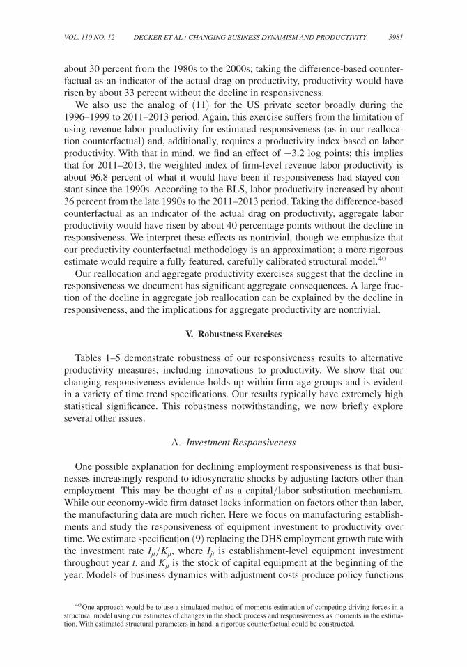
3981DECKER ET AL.: CHANGING BUSINESS DYNAMISM AND PRODUCTIVITYVOL. 110 NO. 12
about 30 percent from the 1980s to the 2000s; taking the difference-based counter-factual as an indicator of the actual drag on productivity, productivity would have risen by about 33 percent without the decline in responsiveness.
We also use the analog of (11) for the US private sector broadly during the 1996–1999 to 2011–2013 period. Again, this exercise suffers from the limitation of using revenue labor productivity for estimated responsiveness (as in our realloca-tion counterfactual) and, additionally, requires a productivity index based on labor productivity. With that in mind, we find an effect of −3.2 log points; this implies that for 2011–2013, the weighted index of firm-level revenue labor productivity is about 96.8 percent of what it would have been if responsiveness had stayed con-stant since the 1990s. According to the BLS, labor productivity increased by about 36 percent from the late 1990s to the 2011–2013 period. Taking the difference-based counterfactual as an indicator of the actual drag on productivity, aggregate labor productivity would have risen by about 40 percentage points without the decline in responsiveness. We interpret these effects as nontrivial, though we emphasize that our productivity counterfactual methodology is an approximation; a more rigorous estimate would require a fully featured, carefully calibrated structural model.40
Our reallocation and aggregate productivity exercises suggest that the decline in responsiveness we document has significant aggregate consequences. A large frac-tion of the decline in aggregate job reallocation can be explained by the decline in responsiveness, and the implications for aggregate productivity are nontrivial.
V. Robustness Exercises
Tables 1–5 demonstrate robustness of our responsiveness results to alternative productivity measures, including innovations to productivity. We show that our changing responsiveness evidence holds up within firm age groups and is evident in a variety of time trend specifications. Our results typically have extremely high statistical significance. This robustness notwithstanding, we now briefly explore several other issues.
A. Investment Responsiveness
One possible explanation for declining employment responsiveness is that busi-nesses increasingly respond to idiosyncratic shocks by adjusting factors other than employment. This may be thought of as a capital/labor substitution mechanism. While our economy-wide firm dataset lacks information on factors other than labor, the manufacturing data are much richer. Here we focus on manufacturing establish-ments and study the responsiveness of equipment investment to productivity over time. We estimate specification (9) replacing the DHS employment growth rate with the investment rate I jt / K jt , where I jt is establishment-level equipment investment throughout year t , and K jt is the stock of capital equipment at the beginning of the year. Models of business dynamics with adjustment costs produce policy functions
40 One approach would be to use a simulated method of moments estimation of competing driving forces in a structural model using our estimates of changes in the shock process and responsiveness as moments in the estima-tion. With estimated structural parameters in hand, a rigorous counterfactual could be constructed.

3982 THE AMERICAN ECONOMIC REVIEW DECEMBER 2020
and intuition for capital investment that are similar to the policy functions and intu-ition for employment growth.41
We estimate the investment responsiveness specification separately for high-tech and non-tech establishments, and for brevity we report only the regression in which the time functions T y ( a jt , t) and T m ( a jt , t) are specified as decade-specific coefficients (the last element in (8)). Table 6 reports the results based again on our preferred TFP measure, TFPS, standing in for a jt . In the first column, among all industries we see rising investment responsiveness from the 1980s to the 1990s followed by a drop in the 2000s. This pattern is consistent with capital/labor substitution between the 1980s and 1990s while employment responsiveness was falling, after which invest-ment joins employment in becoming less responsive in the 2000s. The non-tech column is similar.
The high-tech column is striking: while responsiveness among high-tech estab-lishments was stronger than the rest of the manufacturing sector during the 1980s, by the 2000s it is far weaker than the rest of manufacturing and is in fact no longer statistically significant (though the difference between the 1990s and the 2000s is significant). We observe a similar pattern among both young and mature firms. In other words, productivity selection for growth via equipment investment appears completely absent in high-tech manufacturing during the 2000s. Similarly to our employment results, we can quantify investment responsiveness in terms of the differential between high-productivity establishments (those that are one standard deviation more productive than their industry mean) and average (within-industry) establishments. Among high-tech young firm establishments, this differential in investment rates rose from 4.8 percentage points to 7.4 percentage points from the 1980s to the 1990s before falling close to zero in the 2000s.
In recent years researchers have given increasing focus to intangible capital (e.g., Corrado, Hulten, and Sichel 2009; Haskel and Westlake 2017). Weakening respon-siveness of employment and equipment investment could have been accompanied by changes in the responsiveness of intangible capital investment, which we cannot measure with our data. For example, high-productivity firms may be investing more in managerial capabilities (see, e.g., Bloom and Van Reenen 2007). Investment in other forms of intangible capital, such as software or intellectual property, also may play a growing role (e.g., Crouzet and Eberly 2018).
B. Worker Hours
Another potential explanation for declining employment responsiveness is that businesses may increasingly adjust hours per worker in response to shocks, offset-ting the decline in employment responsiveness. There are multiple factors that limit hours per worker as a margin of adjustment (see, e.g., the discussion in Cooper, Haltiwanger, and Willis 2007 and citations therein). Still, we can study this adjust-ment margin for production worker hours in manufacturing.
41 To make results comparable and minimize disclosure issues we use exactly the same specification as (9) except replacing the dependent variable. Unreported specifications where we also control for the initial capital stock each period (allowing such effects to vary over time as with other variables) produce similar results. Also in unreported exercises we find that adding the initial capital stock variable to the employment growth regressions in Table 5 does not materially affect our main results.

3983DECKER ET AL.: CHANGING BUSINESS DYNAMISM AND PRODUCTIVITYVOL. 110 NO. 12
For production workers in manufacturing, we have measures of both total hours and the number of production workers on a quarterly basis. This permits constructing a measure of production hours per worker.42 As noted above, the ASM is represen-tative in the cross section for any given year, but it is not necessarily longitudinally representative, so the time series dimension of our measure of growth in production worker hours faces a similar limitation to our measures of TFP innovations and changes (whereas our employment growth exercises utilize the LBD universe data). With that caveat in mind, we estimate equation (7), replacing the dependent variable with the DHS growth rate of production hours per worker and limiting the sample to longitudinally covered establishments as in certain previous exercises.
The results are in Table 7, where we focus on decade-specific responsiveness coef-ficients and TFPS for parsimony. The responsiveness of hours per worker growth to productivity is small and does not change systematically between the 1980s and the 2000s. An establishment with a one standard deviation higher productivity than its
42 As discussed in online Appendix Section II, for our TFP estimates we construct a measure of total hours for all workers. However, for employment counts of all workers we only have a point-in-time measure for March. Dividing total hours by a point-in-time measure for employment would be a poor measure of hours per worker as it would reflect seasonal variation in employment. The ASM provides the number of production workers in March, June, August, and November; we divide annual total hours by the average of these quarterly numbers.
Table 6—Investment Rate Responsiveness Has Also Weakened (Manufacturing)
Capital investment rate
All industries Non-tech High-tech
Prod × Young × 1980s: λ 80s y 0.0670 0.0668 0.1005
(0.0098) (0.0103) (0.0330)Prod × Young × 1990s: λ 90s
y 0.1768 0.1785 0.1550(0.0139) (0.0147) (0.0312)
Prod × Young × 2000s: λ 00s y 0.1003 0.1048 0.0133a
(0.0092) (0.0086) (0.0281)
Prod × Mature × 1980s: λ 80s m 0.0414 0.0393 0.0746(0.0068) (0.0071) (0.0283)
Prod × Mature × 1990s: λ 90s m 0.1151 0.1144 0.1294(0.0082) (0.0087) (0.0200)
Prod × Mature × 2000s: λ 00s m 0.0619 0.0658 −0.0020a
(0.0051) (0.0053) (0.0194)
p-value: λ 80s y = λ 90s
y 0.00 0.00 0.22
p-value: λ 80s y = λ 00s
y 0.00 0.00 0.04
p-value: λ 90s y = λ 00s
y 0.00 0.00 0.00
p-value: λ 80s m = λ 90s m 0.00 0.00 0.12
p-value: λ 80s m = λ 00s m 0.02 0.00 0.03
p-value: λ 90s m = λ 00s m 0.00 0.00 0.00
Observations (thousands) 2,375 2,239 136
Notes: Equipment investment. Manufacturing only with TFPS productivity concept. High-tech industries defined as in Hecker (2005). All coefficients statistically significant with p < 0.05 (and almost always with p < 0.01 ) unless otherwise noted. All regressions include controls described in equation (7) and related text.
a Not statistically significant.
Sources: LBD, ASM-CM, and author calculations

3984 THE AMERICAN ECONOMIC REVIEW DECEMBER 2020
industry mean has about a half percentage point higher growth in hours per worker in both the 1980s and the 2000s. During the 1990s, the relationship between hours per worker growth and productivity is not significant.
The change in the responsiveness of hours per worker to TFPS is much smaller than the analogous change in responsiveness of employment growth reported in Table 1. In Table 1, the responsiveness of employment growth declined by about 9 percentage points from the 1980s to the 2000s while there is no change in the responsiveness of hours per worker growth over the same period. For the change from the 1990s to the 2000s, responsiveness of employment growth declined by about 5 percentage points (Table 1), while responsiveness of hours per worker growth increased by about 1 percentage point. It is apparent that changing respon-siveness on the hours per worker margin cannot mitigate the large decline in the responsiveness of employment growth.
C. Shock Mismeasurement and Dispersion-Dependent Responsiveness
In Section IIIA, we presented evidence that TFP dispersion and revenue labor productivity dispersion are rising, contrary to the “shocks” hypothesis in which declining reallocation might be explained by declining shock dispersion. There are two potential questions about this result. First, some researchers have argued that the rise in productivity dispersion in manufacturing is, in some part, an artifact of increasing measurement error in the ASM establishment sample (Bils, Klenow, and Ruane 2020). We have already shown evidence that this is not likely, since rising dispersion of revenue labor productivity is evident even in RE-LBD administrative data. However, there might still be concern that our finding of declining responsive-ness reflects increasingly mismeasured productivity (e.g., from mismeasured inputs like capital). Second, in the case of non-convex adjustment costs, responsiveness varies with productivity dispersion in a manner that complicates the “shocks versus responsiveness” dichotomy (see online Appendix Section I).
Table 7—Responsiveness of Hours per Worker Growth Is Small and Little Changed
TFPS
Prod × 1980s: λ 80s 0.0110(0.0044)
Prod × 1990s: λ 90s 0.0012a
(0.0035)Prod × 2000s: λ 00s 0.0102
(0.0028)
p-value: λ 80s = λ 90s 0.08p-value: λ 80s = λ 00s 0.87p-value: λ 90s = λ 00s 0.04
Observations (thousands) 854
Notes: Regression of hours per worker growth on TFPS and controls as described in Section VB. Coefficients are statistically significant with p < 0.01 unless otherwise noted.
a Not statistically significant.
Sources: LBD, ASM-CM, and author calculations

3985DECKER ET AL.: CHANGING BUSINESS DYNAMISM AND PRODUCTIVITYVOL. 110 NO. 12
These two issues are distinct, but both hinge on whether responsiveness is related to measured dispersion. We investigate this question using cross-industry variation in the time series of shock dispersion. In the ASM, we classify 4-digit NAICS industries into three groups based on terciles of the 1980s–2000s change in within-industry TFPS dispersion. The top tercile of industries saw a mean change of +0.11 in the standard deviation of TFPS; the middle tercile saw a mean change of +0.04, and the bottom tercile saw a mean change of −0.02. We interact dummy indicators of these terciles with our responsiveness coefficients in a regression oth-erwise similar to those reported in the first column of Table 1, focusing on the linear trend variable to avoid the proliferation of coefficients. These results are shown in the first column of Table 8. Focusing on the coefficients interacting productivity with tercile indicators and the trend, we do not find that the responsiveness trend is monotonic in the change in dispersion. The largest downward trend is seen in the middle tercile of industries, while the second-largest downward trend is in the bottom tercile of industries. The top tercile of industries, those with the largest gains in TFPS dispersion, see the smallest downward trend in responsiveness. We cannot reject the hypothesis that the trends in the top and bottom terciles are equal, but we (marginally) reject the hypothesis of equality between the top and middle terciles. These results provide evidence that the decline in responsiveness is not driven by changes in measured dispersion.
D. Changing Shock Persistence
Panel D of Figure 3 shows the persistence of productivity shocks has declined from the 1980s to the 2000s. We view these changes as modest. However, in models of labor adjustment costs such as ours, a decline in shock persistence can, by itself, reduce responsiveness as firms are reluctant to pay a cost to respond to shocks that are likely to be transitory. We again exploit industry variation to explore whether declining shock persistence might explain declining responsiveness.43 We divide 4-digit NAICS industries (within manufacturing) into terciles based on their change in persistence from the 1980s to the 2000s, where persistence is measured as the estimated AR(1) coefficient in the TFPS process. The top tercile has a mean change of +0.10, the middle tercile has a mean change of −0.02, and the bottom tercile has a mean change of −0.11. As in our dispersion exercises in the previous subsection, we interact tercile dummies with productivity and time trends to allow responsive-ness trends to vary across the persistence terciles (and, again, we focus on the linear trend to avoid coefficient proliferation).
The results are reported in the second column of Table 8. At the industry level, the decline in responsiveness is not monotonic in the change in persistence. The largest decline in responsiveness is seen in the middle persistence tercile, followed by the bottom tercile then the top tercile. We cannot reject the hypothesis that the bottom and top persistence terciles see the same decline in responsiveness. Moreover, if declining persistence were to explain declining responsiveness, we would expect establishments in the top tercile, in which persistence actually rose, to see rising
43 Here we note, yet again, that ASM data are not optimal for calculating longitudinal variables like persistence.

3986 THE AMERICAN ECONOMIC REVIEW DECEMBER 2020
responsiveness over time, rather than the negative trend we observe. Changing shock persistence does not appear to be driving our findings on declining responsiveness.
E. Employment Measurement Error and Division Bias
Initial employment is a control in our responsiveness regressions but also enters the calculation of measured employment growth. This raises questions about division bias in the presence of measurement error in employment, which could introduce bias in our estimated responsiveness coefficients when using employment growth as the dependent variable.
We first note that our analysis of exit uses a dependent variable equal to 1 if a plant or firm exits between t and t + 1 based on productivity and employment measures in t . Measurement error in initial employment does not cause division bias in this specification. Our results on exit show a systematic pattern of declining responsiveness.
For the specifications with the DHS growth rate as the dependent variable, we explore the potential consequences of measurement error in employment in period t
Table 8—Responsiveness Does Not Vary Systematically with Industry Shock Dispersion or Persistence
Responsiveness by dispersion tercilea
Responsiveness by persistence tercileb
Prod × Bottom tercile 0.2792 0.2771(0.0120) (0.0112)
Prod × Middle tercile 0.3372 0.3338(0.0144) (0.0139)
Prod × Top tercile 0.2782 0.2659(0.0160) (0.0153)
Prod × Bottom tercile × trend −0.0036 −0.0032(0.0006) (0.0006)
Prod × Middle tercile × trend −0.0045 −0.0045(0.0008) (0.0007)
Prod × Top tercile × trend −0.0026 −0.0026(0.0007) (0.0008)
p-value: Prod × Bottom tercile = Prod × Middle tercile 0.00 0.00p-value: Prod × Middle tercile = Prod × Top tercile 0.00 0.00p-value: Prod × Bottom tercile = Prod × Top tercile 0.95 0.50
p-value: Prod × Bottom × trend = Prod × Middle × trend 0.32 0.09p-value: Prod × Middle × trend = Prod × Top × trend 0.05 0.05p-value: Prod × Bottom × trend = Prod × Top × trend 0.25 0.47
Observations (thousands) 2,375 2,375
Notes: All regression coefficients are statistically significant with p < 0.01 . Bottom, middle, and top terciles refer to the change in TFPS dispersion (first column) or persistence (second column), where top is the highest change and bottom is the lowest change.
a The mean industry-level changes in dispersion are −0.02, +0.04, and +0.11 for the bottom, middle, and top terciles, respectively.
b The mean industry-level changes in persistence are −0.11, −0.02, and +0.10 for the bottom, middle, and top terciles, respectively.
Sources: LBD, ASM-CM, and author calculations
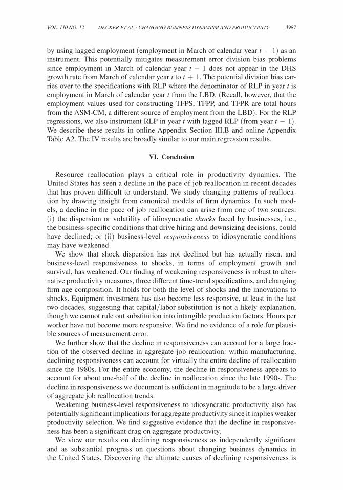
3987DECKER ET AL.: CHANGING BUSINESS DYNAMISM AND PRODUCTIVITYVOL. 110 NO. 12
by using lagged employment (employment in March of calendar year t − 1 ) as an instrument. This potentially mitigates measurement error division bias problems since employment in March of calendar year t − 1 does not appear in the DHS growth rate from March of calendar year t to t + 1 . The potential division bias car-ries over to the specifications with RLP where the denominator of RLP in year t is employment in March of calendar year t from the LBD. (Recall, however, that the employment values used for constructing TFPS, TFPP, and TFPR are total hours from the ASM-CM, a different source of employment from the LBD). For the RLP regressions, we also instrument RLP in year t with lagged RLP (from year t − 1 ). We describe these results in online Appendix Section III.B and online Appendix Table A2. The IV results are broadly similar to our main regression results.
VI. Conclusion
Resource reallocation plays a critical role in productivity dynamics. The United States has seen a decline in the pace of job reallocation in recent decades that has proven difficult to understand. We study changing patterns of realloca-tion by drawing insight from canonical models of firm dynamics. In such mod-els, a decline in the pace of job reallocation can arise from one of two sources: (i) the dispersion or volatility of idiosyncratic shocks faced by businesses, i.e., the business-specific conditions that drive hiring and downsizing decisions, could have declined; or (ii) business-level responsiveness to idiosyncratic conditions may have weakened.
We show that shock dispersion has not declined but has actually risen, and business-level responsiveness to shocks, in terms of employment growth and survival, has weakened. Our finding of weakening responsiveness is robust to alter-native productivity measures, three different time-trend specifications, and changing firm age composition. It holds for both the level of shocks and the innovations to shocks. Equipment investment has also become less responsive, at least in the last two decades, suggesting that capital/labor substitution is not a likely explanation, though we cannot rule out substitution into intangible production factors. Hours per worker have not become more responsive. We find no evidence of a role for plausi-ble sources of measurement error.
We further show that the decline in responsiveness can account for a large frac-tion of the observed decline in aggregate job reallocation: within manufacturing, declining responsiveness can account for virtually the entire decline of reallocation since the 1980s. For the entire economy, the decline in responsiveness appears to account for about one-half of the decline in reallocation since the late 1990s. The decline in responsiveness we document is sufficient in magnitude to be a large driver of aggregate job reallocation trends.
Weakening business-level responsiveness to idiosyncratic productivity also has potentially significant implications for aggregate productivity since it implies weaker productivity selection. We find suggestive evidence that the decline in responsive-ness has been a significant drag on aggregate productivity.
We view our results on declining responsiveness as independently significant and as substantial progress on questions about changing business dynamics in the United States. Discovering the ultimate causes of declining responsiveness is

3988 THE AMERICAN ECONOMIC REVIEW DECEMBER 2020
important but beyond the scope of this paper. Our model framework suggests that changing firm-level behavior, rather than a more tranquil profitability environment, should be the focus of further research; for example, rising factor adjustment costs or changes in the relationship between revenue distortions and business-level pro-ductivity can readily produce both declining responsiveness and the rising disper-sion of revenue-based productivity measures we observe. This could be the result of regulatory changes that affect the cost of hiring or downsizing; alternatively changes in the economic environment that are more interpretable in the “correlated wedges” framework could be to blame. As examples of the former, Davis and Haltiwanger (2014) focus on changes in employment-at-will doctrines in the US judicial system, rising prevalence of occupational licensing, increasing use of non-competes even in sectors such as fast-food restaurants, and potential indirect factors (such as zoning) that impair geographic labor mobility. Alternatively, the “correlated wedges” inter-pretation could accommodate a role for rising product market power (as studied by De Loecker, Eeckhout, and Unger 2020) or labor market power, as firms may absorb high productivity shocks through higher markups.
Our estimated negative effects of declining responsiveness on aggregate produc-tivity are noteworthy. However, we also acknowledge that reallocation is costly. While job reallocation can facilitate job growth and job-to-job transitions, an import-ant source of wage gains, job destruction imposes profound costs on workers, fam-ilies, and communities. Optimal policies for labor and other markets must balance these considerations against the benefits of productivity-enhancing reallocation for overall living standards. Identifying the source of declining responsiveness is a crit-ical avenue for future research.
REFERENCES
Andrews, Dan, Chiara Criscuolo, and Peter N. Gal. 2015. “Frontier Firms, Technology Diffusion and Public Policy: Micro Evidence from OECD Countries.” The Future of Productivity: Main Back-ground Papers.
Autor, David, David Dorn, Lawrence Katz, Christina Patterson, and John Van Reenen. Forthcoming. “The Fall of the Labor Share and the Rise of Superstar Firms.” Quarterly Journal of Economics.
Bachmann, Rüdiger, and Christian Bayer. 2013. “‘Wait-and-See’ Business Cycles?” Journal of Mon-etary Economics 60 (6): 704–19.
Baily, Martin Neil, Charles Hulten, and David Campbell. 1992. “Productivity Dynamics in Manufac-turing Plants.” Brookings Papers on Economic Activity: Microeconomics: 187–249.
Barro, Robert J. 1972. “A Theory of Monopolistic Price Adjustment.” Review of Economic Studies 39 (1): 17–26.
Barth, Erling, Alex Bryson, James C. Davis, and Richard Freeman. 2016. “It’s Where You Work: Increases in the Dispersion of Earnings across Establishments and Individuals in the United States.” Journal of Labor Economics 34 (2): S67–97.
Berger, David, and Joseph Vavra. 2019. “Shocks vs. Responsiveness: What Drives Time-Varying Dis-persion.” Journal of Political Economy 127 (5): 2104–42.
Bils, Mark, Peter J. Klenow, and Cian Ruane. 2020. “Misallocation or Mismeasurement?” NBER Working Paper 26711.
Blackwood, G. Jacob, Lucia S. Foster, Cheryl A. Grim, John Haltiwanger and Zoltan Wolf. Forthcom-ing. “Macro and Micro Dynamics of Productivity: From Devilish Details to Insights.” American Eco-nomic Journal: Macroeconomics.
Bloom, Nicholas. 2009. “The Impact of Uncertainty Shocks.” Econometrica 77 (3): 623–85.Bloom, Nicholas, Max Floetotto, Nir Jaimovich, Itay Saporta-Eksten, and Stephen J. Terry. 2018.
“Really Uncertain Business Cycles.” Econometrica 86 (3): 1031–65.Bloom, Nicholas, and John Van Reenen. 2007. “Measuring and Explaining Management Practices
across Firms and Countries.” Quarterly Journal of Economics 122 (4): 1351–408.

3989DECKER ET AL.: CHANGING BUSINESS DYNAMISM AND PRODUCTIVITYVOL. 110 NO. 12
Caballero, Ricardo J., Eduardo M. R. A. Engel, and John Haltiwanger. 1997. “Aggregate Employment Dynamics: Building from Microeconomic Evidence.” American Economic Review 87 (1): 115–37.
Cooper, Russell W., and John C. Haltiwanger. 2006. “On the Nature of Capital Adjustment Costs.” Review of Economic Studies 73 (3): 611–33.
Cooper, Russell, John Haltiwanger, and Jonathan L. Willis. 2007. “Search Frictions: Matching Aggre-gate and Establishment Observations.” Journal of Monetary Economics 54: S56–78.
Corrado, Carol, Charles Hulten, and Daniel Sichel. 2009. “Intangible Capital and U.S. Economic Growth.” Review of Income and Wealth 55 (3): 661–85.
Crouzet, Nicolas, and Janice Eberly. 2018. “Intangibles, Investment, and Efficiency.” AEA Papers and Proceedings 108: 426–31.
Davis, Steven J., and John Haltiwanger. 2014. “Labor Market Fluidity and Economic Performance.” NBER Working Paper 20479.
Davis, Steven J., John Haltiwanger, Ron Jarmin, and Javier Miranda. 2007. “Volatility and Disper-sion in Business Growth Rates: Publicly Traded versus Privately Held Firms.” In NBER Macroeco-nomics Annual 2006, Vol. 21, edited by Daron Acemoglu, Kenneth Rogoff, and Michael Woodford, 107–56. Cambridge, MA: MIT Press.
Davis, Steven J., John C. Haltiwanger, and Scott Schuh. 1996. Job Creation and Destruction. Cam-bridge, MA: MIT Press.
Decker, Ryan, John Haltiwanger, Ron Jarmin, and Javier Miranda. 2014. “The Role of Entrepre-neurship in US Job Creation and Economic Dynamism.” Journal of Economic Perspectives 28 (3): 3–24.
Decker, Ryan A., John Haltiwanger, Ron S. Jarmin, and Javier Miranda. 2016a. “Declining Business Dynamism: Implications for Productivity?” Hutchins Center Working Paper 23.
Decker, Ryan A., John Haltiwanger, Ron S. Jarmin, and Javier Miranda. 2016b. “Where Has All the Skewness Gone? The Decline in High-Growth (Young) Firms in the U.S.” European Economic Review 86: 4–23.
Decker, Ryan A., John Haltiwanger, Ron S. Jarmin, and Javier Miranda. 2017. “Declining Dyna-mism, Allocative Efficiency, and the Productivity Slowdown.” American Economic Review 107 (5): 322–26.
Decker, Ryan A., John C. Haltiwanger, Ron S. Jarmin, and Javier Miranda. 2018. “Changing Business Dynamism and Productivity: Shocks vs. Responsiveness.” NBER Working Paper 24236.
Decker, Ryan A., John Haltiwanger, Ron S. Jarmin, and Javier Miranda. 2020. “Replication Data for: Changing Business Dynamism and Productivity: Shocks versus Responsiveness.” American Eco-nomic Association [publisher], Inter-university Consortium for Political and Social Research [dis-tributor]. https://doi.org/10.3886/E120432V1.
De Loecker, Jan, Jan Eeckhout and Gabriel Unger. 2020. “The Rise of Market Power and the Macro-economic Implications.” Quarterly Journal of Economics 135 (2): 561–644.
De Loecker, Jan, Pinelopi K. Goldberg, Amit K. Khandelwal, and Nina Pavcnik. 2016. “Prices, Mark-ups, and Trade Reform.” Econometrica 84 (2): 445–510.
Edmond, Chris, Virgiliu Midrigan, and Daniel Yi Xu. 2018. “How Costly Are Markups?” NBER Working Paper 24800.
Elsby, Michael W. L., and Ryan Michaels. 2013. “Marginal Jobs, Heterogeneous Firms, and Unem-ployment Flows.” American Economic Journal: Macroeconomics 5 (1): 1–48.
Eslava, Marcela, and John C. Haltiwanger. 2020. “The Life-Cycle Growth of Plants: The Role of Pro-ductivity, Demand and Wedges.” NBER Working Paper 27184.
Fernald, John. 2014. “Productivity and Potential Output before, during, and after the Great Recession.” In NBER Macroeconomics Annual 2014, Vol. 29, edited by Jonathan A. Parker and Michael Wood-ford, 1–51. Cambridge, MA: MIT Press.
Fort, Teresa, and Shawn Klimek. 2016. “The Effects of Industry Classification Changes on US Employment Composition.” Unpublished.
Foster, Lucia, Cheryl Grim, and John Haltiwanger. 2016. “Reallocation in the Great Recession: Cleansing or Not?” Journal of Labor Economics 34 (1): S293-331.
Foster, Lucia, John Haltiwanger, and C. J. Krizan. 2001. “Aggregate Productivity Growth: Lessons from Microeconomic Evidence.” In New Developments in Productivity Analysis, edited by Charles R. Hulten, Edwin R. Dean, and Michael J. Harper, 303–63. Chicago: University of Chicago Press.
Foster, Lucia, John Haltiwanger, and Chad Syverson. 2008. “Reallocation, Firm Turnover, and Effi-ciency: Selection on Productivity or Profitability?” American Economic Review 98 (1): 394–425.
Gopinath, Gita, Sebnem Kalemli-Özcan, Loukas Karabarbounis, and Carolina Villegas-Sanchez. 2017. “Capital Allocation and Productivity in South Europe.” Quarterly Journal of Economics 132 (4): 1915–67.

3990 THE AMERICAN ECONOMIC REVIEW DECEMBER 2020
Guzman, Jorge, and Scott Stern. 2016. “The State of American Entrepreneurship: New Estimates of the Quantity and Quality of Entrepreneurship for 15 US States, 1988–2014.” Unpublished.
Haltiwanger, John, Ian Hathaway, and Javier Miranda. 2014. “Declining Business Dynamism in the U.S. High-Technology Sector.” Kauffman Foundation.
Haltiwanger, John, Ron S. Jarmin, Robert Kulick, and Javier Miranda. 2017. “High Growth Young Firms: Contribution to Job, Output, and Productivity Growth.” In Measuring Entrepreneurial Busi-nesses: Current Knowledge and Challenges, edited by John Haltiwanger et al. Chicago: University of Chicago Press.
Haltiwanger, John, Ron S. Jarmin, and Javier Miranda. 2013. “Who Creates Jobs? Small versus Large versus Young.” Review of Economics and Statistics 95 (2): 347–61.
Haskel, Jonathan, and Stian Westlake. 2017. Capitalism without Capital: The Rise of the Intangible Economy. Princeton, NJ: Princeton University Press.
Hecker, Daniel. 2005. “High-Technology Employment: A NAICS-Based Update.” Monthly Labor Review 128 (7): 57–72.
Hopenhayn, Hugo A. 1992. “Entry, Exit, and Firm Dynamics in Long-Run Equilibrium.” Economet-rica 60 (5): 1127–50.
Hopenhayn, Hugo, and Richard Rogerson. 1993. “Job Turnover and Policy Evaluation: A General Equilibrium Analysis.” Journal of Political Economy 101 (5): 915–38.
Hottman, Colin J., Stephen J. Redding, and David E. Weinstein. 2016. “Quantifying the Sources of Firm Heterogeneity.” Quarterly Journal of Economics 131 (3): 1291–1364
Hsieh, Chang-Tai, and Peter J. Klenow. 2009. “Misallocation and Manufacturing TFP in China and India.” Quarterly Journal of Economics 124 (4): 1403–48.
Hyatt, Henry R., and James R. Spletzer. 2013. “The Recent Decline in Employment Dynamics.” IZA Journal of Labor Economics 2: 5.
Ilut, Cosmin, Matthias Kehrig, and Martin Schneider. 2018. “Slow to Hire, Quick to Fire: Employment Dynamics with Asymmetric Responses to News.” Journal of Political Economy 126 (5): 2011–71.
Jovanovic, Boyan. 1982. “Selection and the Evolution of Industry.” Econometrica 50 (3): 649–70.Karahan, Fatih, Benjamin Pugsley, and Aysegül Sahin. 2018. “Demographic Origins of the Startup
Deficit.” Unpublished. Kehrig, Matthias, and Nicolas Vincent. 2017. “Growing Productivity without Growing Wages: The
Micro-Level Anatomy of the Aggregate Labor Share Decline.” ERID Working Paper 244.Kehrig, Matthias, and Nicolas Vincent. 2020. “The Micro-Level Anatomy of the Labor Share Decline.”
NBER Working Paper 25275.Molloy, Raven, Christopher L. Smith, Riccardo Trezzi, and Abigail Wozniak. 2016. “Understanding
Declining Fluidity in the U.S. Labor Market.” Brookings Papers on Economic Activity 47: 183–237.Olley, G. Steven, and Ariel Pakes. 1996. “The Dynamics of Productivity in the Telecommunications
Equipment Industry.” Econometrica 64 (6): 1263–97.Pugsley, Benjamin, Petr Sedlácek, and Vincent Sterk. 2017. “The Nature of Firm Growth.” CFM Dis-
cussion Paper 1737.Syverson, Chad. 2004. “Product Substitutability and Productivity Dispersion.” Review of Economics
and Statistics 86 (2): 534–50.Syverson, Chad. 2011. “What Determines Productivity?” Journal of Economic Literature 49 (2): 326–
65.Vavra, Joseph. 2014. “Inflation Dynamics and Time-Varying Volatility: New Evidence and an Ss Inter-
pretation.” Quarterly Journal of Economics 129 (1): 215–58.Wooldridge, Jeffrey M. 2009. “On Estimating Firm-Level Production Functions Using Proxy Variables
to Control for Unobservables.” Economics Letters 104 (3): 112–14.