Do SBA Loans Create Jobs?

Estimates from Universal Panel Data and Longitudinal Matching Methods

J. David Brown and John S. Earle*

September 2012

Abstract

This paper reports estimates of the effects of the Small Business Administration (SBA)

7(a) and 504 loan programs on employment. The database links a complete list of all SBA loans

in these programs to universal data on all employers in the U.S. economy from 1976 to 2010.

Our method is to estimate firm fixed effect regressions using matched control groups for the

SBA loan recipients we have constructed by matching exactly on firm age, industry, year, and

pre-loan size, plus kernel-based matching on propensity scores estimated as a function of four

years of employment history and other variables. The results imply positive average effects on

loan recipient employment of about 25 percent or 3 jobs at the mean. Including loan amount, we

find little or no impact of loan receipt per se, but an increase of about 5.4 jobs for each million

dollars of loans. Examining loans received only in high growth county-years (average growth of

22 percent), where most small firms should have excellent growth potential, we find similar

effects, implying that the estimates are not driven by differential demand conditions across firms.

Results are also similar regardless of distance of control from recipient firms, suggesting only a

very small role for displacement effects. In all these cases, the results pass a “pre-program”

specification test, where controls and treated firms look similar in the pre-loan period. Other

specifications, such as those using only matching or only regression imply somewhat higher

effects, but they fail the pre-program test.

* Brown (j.david.brown@census.gov): Center for Economic Studies–U.S. Census Bureau. Earle (earle@gmu.edu):

School of Public Policy–George Mason University and Central European University. We thank Zoltan Acs, Sergey

Lychagin, Gabor Kezdi, and participants in presentations at the Southern Economic Association Annual Meetings,

the Comparative Analysis of Enterprise Data Conference in Nuremberg, George Mason University, Central

European University, and the Small Business Administration (SBA) for helpful comments on preliminary results.

We also thank the SBA for providing the list of loans we use in the analysis. Any opinions and conclusions

expressed herein are those of the authors and do not necessarily reflect the views of the U.S. Census Bureau. All

results have been reviewed to ensure that no confidential information on individual firms is disclosed.

1

1. Introduction

The “strategic goal” of the Small Business Administration (SBA) is “growing businesses

and creating jobs.”1 The urgency of this mission has increased during the current slow recovery

and high unemployment in the U.S. Nearly all political groups have reached a rare agreement

that small businesses are the primary source of job creation, and the budget of the SBA has

steadily increased, reaching “all-time records in the Agency’s history, with over $30 billion in

lending support to 60,000 small businesses in its top two lending programs — 7(a) and 504”

during fiscal year 2011.2

The broad assumption underlying the SBA programs is that easier credit facilitates

growth, but whether the programs increase employment is theoretically ambiguous. Easier

access to finance may overcome credit market imperfections and enable expansion (Stiglitz and

Weiss, 1981). But the causal effect may be attenuated by “substitution effects” (crowding out of

other sources of capital) and the aggregate growth consequences may be reduced by general

equilibrium “displacement effects” (negative spillovers onto competing firms). If capital and

labor are gross substitutes, the effect on employment could even be negative if the loan programs

induce capital-labor substitution. Analyzing the impact of these programs is also empirically

difficult for several reasons: many factors influence employment and growth, there is likely

selection bias (positive or negative) in the awarding of loans, and firm-level microdata have

usually been unavailable.

Perhaps as a result of these difficulties – and despite the prominence of SBA programs,

their large size and high costs, and the many hopes vested in their benefits for business growth –

there have been few attempts to evaluate them using appropriate data and econometric methods.

Unlike labor market training programs, for example, where researchers have long estimated

employment and wage impacts using appropriate micro data and program evaluation methods,

analysts of SBA loans have had to rely on small samples, short time series, or aggregated data

that do not permit the use of recent developments in econometrics (e.g., Imbens and Wooldridge,

2009). Most previous evaluations of small business programs consist of simple comparisons

before and after the policy interventions, with little use of comparison groups of nonrecipients.

The most common unit of observation in SBA studies is a geographic area such as the county,

with outcomes measured as overall employment or per-capita income in the local area; Craig et

al. (2009) review these studies. Many factors affect county-level employment and income, of

course, which makes it difficult to disentangle the effects of a program that is small relative to

the local economy. The SBA itself reports a “performance indicator” – the number of “jobs

supported,” reported in recent years at over 0.5 mln.3 Although the exact calculation of this

1 See http://www.sba.gov/about-sba-info/11572. This goal is the first of three; the other two (which would be even

more difficult to evaluate) are “building an SBA that meets the needs of today’s and tomorrow’s small businesses”

and “serving as the voice for small business.” 2 SBA programs have received strong support both from congress and all recent presidential administrations, and

small businesses are frequently cited as “…the places where most new jobs begin” (President’s Weekly Address,

February 6, 2010). The academic source of this conventional wisdom goes back to Birch (1987), but it has been

questioned by a number of economists, for instance, Davis, Haltiwanger, and Schuh (1996) and most recently by

Haltiwanger, Jarmin, and Miranda (forthcoming). For the budget figures, see http://www.sba.gov/sites/default/

files/files/1-508%20Compliant%20FY%202013%20CBJ%20FY%202011%20APR%281%29.pdf . 3The figure is 583,737 for Fiscal Year 2010 (the most recent provided) in http://www.sba.gov/sites/default/

files/files/2-508%20Compliant%20Appendix%20FY%202012%20CBJ%20FY%202011%20APR%281%29.pdf ,

Appendix 3.

2

indicator is unclear, it seems to be based on summing up the borrowers’ statements on loan

applications concerning their intentions to create or retain jobs.

Our research aims to contribute to the evaluation of these employment impacts by using

much better data than were heretofore available and by applying recent econometric methods

developed for estimating causal effects with such data. We link administrative data on every

SBA 7(a) and 540 program loan to long-panel data on the universe of employers in the U.S.

economy, and we used the linked data to implement a longitudinal matching estimator (e.g.,

Heckman et al., 1997, 1998). The annual panels in our data run from 1976 to 2010 and permit us

to select comparator firms based on age, industry, and several years of employment history, to

control for time and firm-fixed effects, and to measure the evolution of employment before and

after the loans were awarded. We use multiple control groups, differentiated by distance from

the loan-recipients, to assess possible general equilibrium (displacement) effects of the loans.

The paper builds on previous research on small business, finance, and government policy

in several ways. Much of the recent small business controversy in the U.S. has actually not

concerned policy directly, but rather the empirical relationship between business size and

employment growth. Birch’s (1987) claim that small businesses were responsible for most job

creation is widely cited as the basis for government programs supporting this sector, although the

underlying methods have been questioned by Davis, Haltiwanger, and Schuh 1996 (see also

Neumark, Wall, and Zhang 2011, and Haltiwanger, Jarmin, and Miranda forthcoming). But the

size-growth relationship is a different issue from the impact of the programs on business growth

and performance, which is the question relevant for policy and the one we address in this paper.

Evaluating the effects of SBA loans on job creation is also related to macroeconomic

debates on the size of the government spending multiplier (e.g., Ramey 2011). As in this paper,

some of the recent literature on that question uses micro-data (e.g., Parker 2011 and Parker et al.

2011). Our analysis of potential displacement effects is relevant for the question whether

government spending merely reallocates resources across economic agents or whether it also has

an aggregate effect.

Finally, the paper is relevant for the broader theoretical and empirical literature on

finance and growth (Levine 2005). As emphasized in Beck’s (2011) review of the econometric

research, a standard identification problem in that literature is determining the direction of

causality between growth and finance, and despite a long list of empirical studies, the degree to

which financial development promotes economic growth remains controversial. Most studies

use aggregate (typically country-level) data. Those using firm-level data frequently employ

country-level measures of financial development, because of the difficulty of measuring financial

constraints at the firm level; see the controversy over the approach of analyzing the relationship

between investment and cash flow (Hubbard 1998). By contrast, in this paper we are able to

analyze a specific policy intervention varying at the firm level, which may be a unique

contribution to this literature.4

Section 2 describes the SBA programs we analyze. Section 3 describes the data,

including the several matched control samples. Section 4 outlines our evaluation methodology.

Section 5 provides results, and Section 6 concludes the paper with a summary of results and

caveats.

4 Beck (2011) concludes his review with a call for firm-level studies evaluating the growth effects of finance by

analyzing specific policy interventions, which is our purpose in this paper.

3

2. SBA Loan Programs

The SBA has several small business loan guarantee programs. SBA 7A loans not part of a

special subprogram can be for an amount up to $5 million, with a maximum 85 percent SBA

guarantee for loans up to $150,000, and a 75 percent maximum guarantee for higher amounts.5

They are term loans that can be used for expansion/renovation; new construction; purchase of

land, buildings, equipment, fixtures, and lease-hold improvements; working capital; debt

refinancing for compelling reasons; seasonal line of credit; and inventory. Maturity depends on

the ability to repay. Usually loans for working capital and machinery (not to exceed the life of

equipment) have a maturity of 5-10 years, while loans for purchase of real estate can have a term

up to 25 years. The SBA sets maximum loan interest rates, which decrease with loan amount

and increase with maturity. Since December 8, 2004 SBA has charged a guaranty fee, which

increases with maturity and loan amount. To qualify, a business must be for-profit; meet SBA

size standards;6 show good character,

7 management expertise, and a feasible business plan; not

have funds available from other sources;8 and be an eligible type of business.

9 The loan

application is sent by the SBA to an independent entity for analysis.

Some 7A programs are more streamlined. Unlike with other 7A loans, in the 7A

Preferred Lender Program (PLP) the SBA delegates the final credit decision and most servicing

and liquidation authority to PLP lenders.10

The SBA’s role is to check loan eligibility criteria.

The SBA selects lenders for PLP status based on their past record with the SBA, including

proficiency in processing and servicing SBA-guaranteed loans. In payment default cases, the

PLP lender agrees to liquidate all business assets before asking the SBA to honor its guaranty.

In the 7A Certified Lender Program (CLP), the SBA promises a loan decision within

three working days on applications handled by CLP lenders.11

Rather than ordering an

independently conducted analysis, the SBA conducts a credit review, relying on the credit

knowledge of the lender’s loan officers. Lenders with a good performance history with SBA

loans may receive CLP status.

5 See http://www.sba.gov/content/7a-terms-conditions.

6 The cut-offs for being a small business vary by NAICS industry. In some industries the criterion is the average

number of employees, with a cut-off ranging from 50 to 1,500. In other industries it is average annual receipts,

ranging from $750,000 to $35.5 million. For many types of financial institutions, the cut-off is $175 million in

assets. See http://www.sba.gov/sites/default/files/files/Size_Standards_Table.pdf. 7 The principals of each applicant firm provide a “Statement of Personal History”, which the SBA uses to determine

if they have shown a willingness and ability to pay their debts and abide by their community’s laws. See

http://www.sba.gov/content/standard-7a-evaluation-criteria. 8 A review is made of both business and personal financial resources. When these resources are deemed excessive,

the business is required to use them in place of part or all of the requested loan proceeds. See

http://www.sba.gov/content/standard-7a-evaluation-criteria. In the lender’s application for an SBA guaranty, the

lender must sign the following statement “Without the participation of SBA to the extent applied for, we would not

be willing to make this loan, and in our opinion the financial assistance applied for is not otherwise available on

reasonable terms.” See http://www.sba.gov/sites/default/files/SBA%20FORM%202301%20B.pdf. 9 This includes engaging in, or proposing to engage in, business in the United States or its possessions; possessing

reasonable owner equity to invest; and using alternative financial resources, including personal assets, before

seeking financial assistance. See http://www.sba.gov/content/7a-eligibility. 10

See http://www.sba.gov/content/steps-participating-plp. 11

See http://www.sba.gov/content/steps-participating-clp.

4

SBA 7A Express loans have a $350,000 maximum loan amount and 50 percent maximum

SBA guaranty.12

Interest rates can be higher than on other 7A loans. Qualified lenders may be

granted authorization by the SBA to make eligibility determinations. The SBA promises a

decision within 36 hours.13

The 504 Loan Program offers loan guarantees up to $5 million or $5.5 million, depending

on the type of business.14

Typically a lender covers 50 percent of the project costs without an

SBA guarantee, a Certified Development Company (CDC) certified by the SBA provides up to

40 percent of the financing (100 percent guaranteed by an SBA-guaranteed debenture), and the

borrower contributes at least 10 percent (the borrower is sometimes required to contribute up to

20 percent). CDCs are nonprofit corporations promoting community economic development via

disbursement of 504 loans. Proceeds may be used for fixed assets or to refinance debt in

connection with an expansion of the business via new or renovated assets. For-profit businesses

with tangible net worth of no more than $15 million and average income of no more than $5

million after federal income taxes in the two years prior to application are eligible. Businesses

must create or retain one job per $65,000 guaranteed by the SBA, with the exception of small

manufacturers, which must create or retain one job per $100,000.

3. Data

We use a database on all 7A and 504 loans guaranteed by the SBA from inception in

1953 through 2009 to identify loan recipients, amounts, and time of receipt. We convert the

SBA-approved loan amounts to real 2010 prices using the annual average Consumer Price Index

from the Bureau of Labor Statistics.15

Loan timing is based on the date the SBA approved the

loan. In order to exclude any firms receiving a disaster loan before their first 7A or 504 loan

from the analysis, we also use a database on all SBA disaster loans from inception through 2009.

We have matched the SBA 7A, 504, and disaster loan data to the Census Bureau’s

employer and non-employer business registers using the following passes: The first is an exact

match on 5-digit zip code, exact match on standardized street address, and exact match on

standardized business name. For those unobservations unmatched after this pass, the second

pass is an exact match on 3-digit zip code, a standardized street address soundex (phonetic

algorithm), and an exact match on standardized business name. The third pass is an exact match

on 5-digit zip code, all of street address allowing for some fuzziness (70 percent sensitivity in

SAS’s DQMATCH software), and business name allowing for some fuzziness. The fourth pass

is an exact match on 5-digit zip code and business name allowing for some fuzziness; and the

fifth pass is place (city) soundex, business name allowing for some fuzziness, street name

allowing for some fuzziness, and street number allowing for some fuzziness. A match from the

first pass is prioritized over the second pass, which is prioritized over the third pass, etc. In a

12

See http://www.sba.gov/content/become-express-lender and http://www.sba.gov/sites/default/files/files/

Loan%20Chart%20Baltimore%20June%202012%20Version%202.pdf. 13

There are several other smaller 7A programs not described here. See http://www.sba.gov/sites/default/files/files/

Loan%20Chart%20Baltimore%20June%202012%20Version%202.pdf. 14

See http://www.sba.gov/content/cdc504-loan-program. 15

This can be downloaded from ftp://ftp.bls.gov/pub/special.requests/cpi/cpiai.txt.

5

first series of passes, the SBA data are matched to business registers from the same year as the

loan. Then they are matched to business registers in the subsequent year, and finally to business

registers in the previous year.

The Census Bureau’s Longitudinal Business Database (LBD) consists of longitudinally

linked employer business registers. The LBD tracks all firms and establishments in the U.S.

non-farm business sector with paid employees on an annual basis in 1976-2010. The SBA loan

match to employer business registers allows us to link the SBA data to the entire LBD. The

LBD contains employment (as of the pay period including March 12th

), annual payroll,

establishment age (calculated based on the first year the establishment appears in the dataset),

state, county, zip code, and industry code. The industry code is a four-digit SIC code through the

year 2001 and a six-digit NAICS code in 2002-2010. We assign each establishment the latitude

and longitude of its 5-digit zip code’s centroid. The Census Bureau has calculated zip code

centroids in the decennial census years of 1990, 2000, and 2010.16

We apply the 1990 centroids

to the years 1976-1990, the 2000 centroids to the year 2000, and the 2010 centroids in 2010. We

linearly interpolate the centroids for 1991-1999 and 2001-2009.

As shown in Table 1, 55.39 percent of the SBA 7A and 504 loans have been matched to

business registers.17

In this study we focus on single-establishment employer businesses

receiving a SBA loan after their first year in operation.18

Among firms receiving multiple SBA

loans, we select the first 7A or 504 loan as the treatment.19

We drop firms with a SBA disaster

loan prior to their first 7A or 504 loan and those receiving their first 7A loan prior to 1977.20

Our

identification method relies heavily on the value of employment in the year prior to loan receipt,

so we drop firms that do not have it in the LBD. Finally, we drop firms for which no suitable

controls are found. Table 1 reports the number of loans dropped as a result of each of these

restrictions.

Potential biases can result from the fact that not all single-establishment employer

businesses receiving a SBA loan after start-up are included in the regression analysis. To get

some feel for the nature of the possible bias, in Table 2 we display descriptive statistics from the

SBA loan applications for four different samples: those reporting to be an existing business and

not matched to any business register, those not in the regressions due to missing employment in

the year prior to the loan, those not in the regressions because no suitable control firms have been

found, and the main regression sample. Those not matched to business registers or which are

missing LBD employment tend to be smaller firms relative to those in the regressions, and more

of them are minority-owned and sole proprietorships or partnerships. In contrast, fewer

16

They can be downloaded at http://www.census.gov/geo/www/gazetteer/gazette.html. 17

Among loans issued to firms identifying themselves on the loan application as existing businesses, the match rate

is somewhat higher, at 59.26 percent. 18

We drop loans issued to an entity that is part of a multi-establishment firm in the loan year or any earlier year.

Though the effects of SBA loans on multi-establishment firms and start-ups are of interest, they require different

identification methods, so we leave them for future research. 19

We limit the analysis to the first loan, as subsequent SBA loans could be influenced by the first loan’s effect. 20

The first 504 loans were issued in 1986. Our identification methods require at least one year of data prior to

receipt of the loan, and the LBD starts in 1976, necessitating dropping 7A loans prior to 1977.

6

recipients without suitable control firms are minority-owned or sole proprietorships or

partnerships, and they are generally larger. More of those without controls are in manufacturing

and fewer are in construction or services. There are nearly nine times as many loans in the not

matched to any business register and missing LBD employment groups as there are in the group

without suitable controls, so overall, the regression sample has higher average employment than

the other groups. This may affect the results if loan effects vary with firm size (a topic of future

research).

Table 3 shows descriptive statistics using variables from the LBD for those SBA firms

matched to it (called treated firms), as well as all other LBD firms (excluding multi-

establishment firms and those ever in a multi-establishment firm in the past). The standard

deviation of employment for firms not receiving SBA loans (i.e., non-treated firms) is much

larger, reflecting the fact that large firms are ineligible for SBA programs. Treated firm median

employment is higher and mean employment is about the same as for non-treated firms,

however, suggesting that SBA loan recipients tend to be larger firms within the small business

sector. Treated firms are younger on average. More treated firms are in manufacturing and

wholesale and retail trade compared to non-treated firms. These differences could affect

employment growth, so a simple comparison of treated and non-treated firm employment growth

is likely to be misleading.

4. Methods

Our goal is to analyze whether there is a causal effect of SBA loan receipt on

employment. Let { } indicate whether firm i receives an SBA loan in year t, and let

be employment at time t+s, , following loan receipt. The employment of the firm if it

hadn’t received a loan is . The loan’s causal effect for firm i at time t+s is defined as

. The value of is not observable, however. We define the average effect of

treatment on the treated as {

} { }

{ }. A counterfactual of the last term, i.e., the average employment outcome

of loan recipients had they not received a loan, can be estimated using the average employment

of non-recipients, { }. This approximation is valid as long as there are no

uncontrolled contemporaneous effects correlated with loan receipt. To help control for such

contemporaneous effects, we use matching techniques to select a control group.

We have taken the following steps to select a control group for the employment

regression sample. As mentioned in Section 3 above, we limit our treated sample to firms in the

LBD that have been single-establishment firms since birth, ones that are at least one year old

when receiving their first SBA loan, those receiving their first SBA 7A or 504 loan in 1977-

2009, those not receiving a SBA disaster loan prior to their first 7A or 504 loan, with non-

missing employment in the LBD in the year before loan receipt, and with no employment

7

outliers in the LBD throughout the 1976-2010 period.21

To be eligible to be a candidate control

firm for a particular treated firm, a firm must have non-missing employment in the year prior to

the treated firm’s loan receipt (which also means it isn’t a new start-up in the year of loan

receipt) and no employment outliers in the LBD; it can never have received an SBA 7A, 504, or

disaster loan at any time between 1953-2010; it can never have been a part of a multi-

establishment firm through the year of loan receipt for the treated firm; it must be in the same

four-digit industry (this is the four-digit SIC code through 2001 and the first four digits of the

NAICS code in 2002-2009) in the treated firm’s loan receipt year, be in the same firm age

category (1-2 years old, 3-5 years old, 6-10 years old, and 11 or more years old) in the treated

firm’s loan receipt year, be in the same firm employment category (1 employee, 2-4 employees,

5-9 employees, 10-19 employees, 20-49 employees, 50-99 employees, and 100 or more

employees) in the year before the treated firm’s loan receipt year. Among firms with nine or

fewer employees in the previous year, we also require the candidate control firm to be located in

the same state (firms with 1-9 employees are much more numerous than ones with more than

nine employees, so we can afford to impose more restrictions on this group). In addition, we

impose a restriction that the ratio of the treated firm’s employment in the previous year to the

control firm’s previous year employment be greater than 0.9 and less than 1.1. This means that

among firms with nine or fewer employees, employment must match exactly.

There are other variables that we would like to match on besides age category, industry,

employment in the year before treatment, and treatment year, but it is difficult to design

matching thresholds for each variable separately, so we reduce this dimensionality problem by

doing propensity score matching. We estimate probit regressions using the sample of treated

firms and their candidate controls.22

A dummy for SBA 7A or 504 loan receipt is regressed on

the log of employment in the year prior to the treated firm’s loan receipt; the square of the log of

employment in the year prior to the treated firm’s loan receipt; the log of employment one year

before minus log employment two years prior to the treated firm’s loan receipt; the log of

employment two years before minus log employment three years prior to the treated firm’s loan

receipt; the log of employment three years before minus log employment four years prior to the

treated firm’s loan receipt; the log of payroll/number of employees in the year prior to the treated

firm’s loan receipt; firm age; firm age squared; and year dummies. We also include dummies for

missing values for the log of employment two years before minus log employment three years

prior to the treated firm’s loan receipt, the log of employment three years before minus log

employment four years prior to the treated firm’s loan receipt, and the log of payroll/number of

employees in the year prior to the treated firm’s loan receipt.23

21

We define the following cases as outliers: an employment increase or decrease of more than ten times between the

first and second year of life or the second-to-last and last year of life; or an employment increase (decrease) of more

than five times followed in the next year by an employment decrease (increase) of more than five times. 22

Treated firms with no candidate controls are dropped at this point. 23

When a firm has a missing value for one of these variables, a zero is imputed.

8

The treated firm observations in the probit regressions are each assigned a weight of ( )

, where N is the total number of firms in the regression and R is the number of treated firms

in the regression. The non-treated firms are assigned a weight of 1. This equalizes the total

weight of the treated firm and non-treated firm groups. The purpose of this weighting is to

produce propensity scores that span a wider range, centered around 0.5 rather than near zero.

We limit the treated and non-treated firms in the employment regression analysis to ones

within a common support, meaning that no propensity score of a treated (non-treated) firm that

we use is higher than the highest non-treated (treated) firm propensity score, and no propensity

score of a treated (non-treated) firm that we use is lower than the lowest non-treated (treated)

firm propensity score. A non-treated firm is included as a control for a particular treated firm if

the ratio of the treated to the non-treated firm’s propensity score is at least 0.95 and not more

than 1.05. Treated firms with no controls meeting all these criteria are not included in the

employment regression analysis. Non-treated firms appear in the employment regressions as

many times as they have treated firms to which they are matched (i.e., this is matching with

replacement). Kernel weights are applied to the controls.24

In the employment regressions, each

control is assigned a final weight of their kernel weight divided by the sum of the kernel weights

for all controls for a particular treated firm, and the treated firm is given a weight of 1. As a

result, the treated firm and all its control firms together receive equal weight.

Propensity score matching relies on a strong assumption of “selection on observables”.

Since our data are longitudinal, we are also able to eliminate unobserved, time-invariant

differences in employment through difference-in-differences (DID) regression specifications.

The employment regression specifications take the following form:

,

where i indexes firms from 1 to I, j indexes from 1 to R the treated firms to which the firm is a

control,25

and t indexes the years from 1 to T. is a 1 x 66 vector of event time dummies.

Designating τ as the index of event time, the number of years since the treated firm received its

first SBA loan, such that in the pre-loan years, in

the year of loan receipt, and in the post-loan years.26

is a 1 x 35 vector of year

dummies, is a fixed effect for each firm for each treated firm to which it is matched, and

is an idiosyncratic error.27

In alternative specifications, is the firm’s employment and the

natural logarithm of the firm’s employment.

24 The kernel weight is (

(

)

)

, where tr is a subscript for the treated firm, and ntr is a

subscript for the non-treated firm. 25

For treated firms, i=j. 26

These event time dummies, which are sometimes non-zero for all firms, in conjunction with , which are

sometimes non-zero only for treated firms, are necessary to make these DID regressions. 27

The standard errors are cluster-adjusted by firm. We have also bootstrapped some specifications, and the standard

errors are similar to those reported here.

9

is a vector of SBA loan treatment measures, and are the loan treatment effects of

interest. We estimate several alternative specifications of . The simplest specifications

include a post-loan dummy, which for treated firms is equal to 1 in the year after receipt of the

first SBA loan and in all subsequent years. Others include the post-loan dummy interacted with

the amount of the first SBA loan, expressed in $thousands, or the post-loan dummy interacted

with the difference between the logarithm of the loan amount and the mean of the log loan

amount among treated firms in the regression.28

Some specifications include both post-loan

dummies and their interactions with loan amount or the difference between the log loan amount

and the mean, and some also include squared terms for the loan amount or the difference

between the log loan amount and the mean. We also estimate dynamic specifications including

treated-firm-specific dummy variables for the years before and after first SBA loan receipt. For

treated firms, these dummy variables take on identical values to the event time dummies

described above, while for non-treated control firms, they are always zero.

Table 4 shows the number of treated firms, number of control firm-treated firm

combinations, the number of pre-treatment and post-treatment firm-years for treated firms, and

the number of pre-treatment and post-treatment years for control firm-treated firm combinations.

On average there are several years of data on each treated and control firm before and after

treatment, the former facilitating control for pre-treatment differences, and the latter allowing us

to study long-run treatment effects. Note that treated firms have more post-treatment years on

average, which indicates a higher survival propensity.

The reliability of propensity score matching depends on whether, conditional on the

propensity score, the potential outcomes and are independent of treatment incidence. The

assumption of independence conditional on observables depends on the pre-treatment variables

being balanced between the treated and control groups. We evaluate this in two ways – by

performing a standardized difference (or bias) test for the main variables included in the

matching probit regressions, and by analyzing the pre-treatment event-time dynamics (see

Section 5). Table 5 reports the means of the main variables included in the matching probit

regressions for four different samples: all treated firms, all non-treated firms, treated firms

included in the employment regressions, and controls included in the employment regressions.

Treated firm employment and average wage are substantially larger than for non-treated firms

prior to matching, and treated firms experience more employment growth in the four years prior

to treatment. After matching, these differences are negligible. The standardized difference

measures confirm this: employment, employment growth, and wage biases are reduced by over

89 percent, while age bias is reduced by 38 percent.29

None of the biases are close to being large

after matching.30

28

If a firm received multiple SBA loans in the year, the loan amounts are combined. 29

The mean age is very similar in the total treated and total non-treated samples, leaving little scope for

improvement through matching. 30

Rosenbaum and Rubin (1985) consider a value of 20 to be large.

10

5. Results

Table 6 contains basic results for specifications with log(employment) as the dependent

variable. The first column is the simplest difference-in-difference (DiD) specification, where the

variable of interest is the Postloan dummy (treatment dummy during the postloan period), and

the result implies an average effect of about 25 percent increase in employment associated with

receiving the loan. Given that average employment is 13 to 15 in our samples, this implies an

average gain of 3-4 jobs in the treated firms relative to an estimated counterfactual of non-

treatment. The other columns in Table 6 allow the effect to vary with log(Loan Amount),

demeaned in the sample so that the Postloan dummy represents the effect at the sample mean,

and the log(Loan Amount) is set to zero for nontreated firms and years. The results suggest that

doubling Loan Amount increases employment by about one job, with some concavity in the

estimated relationship. This result bears much more analysis, however, as it may well reflect

heterogeneous loan effects by firm size, which is likely correlated with loan size, a topic in our

plans for future research.

Next we study the dynamics of loan effects on employment in event time. As described

in the previous section, we can estimate separate effects by years normalized around the loan

year. Grouping together all years five and more years before the loan as the base period (a

normalization is necessary because of the inclusion of firm fixed effects), we permit the

estimated coefficient to vary for each year from four years before to 10+ years after the loan.

Examining the dynamics of the estimates prior to the loan provides a Heckman-Hotz (1989)

“pre-program test” of the specification: if we observe large differences between the treated and

control firms prior to the loan, and particularly if we observe differing trends, then this would be

symptomatic of selection bias, even conditioning on our matching and regression procedures.

Concerning the postloan period, the results in Table 6 assume a constant loan effect in the

postloan period, but an interesting question is whether the estimate is averaging an initial jump in

employment that falls later on, or whether the employment gain is sustained in the longer term.

Figure 2 contains the results from estimating these dynamics. We observe only tiny

differences between the treated and control firms in the preloan period. There is a slight

tendency for worse performance of treated relative to control firms: compared to five years and

more before the loan, employment falls about 3 percent in treated firms relative to controls. But

this difference is trivial compared with the big jumps we estimate in the loan year and year

following: about 20 percent total. The jump in the loan year may be explained by anticipatory

hiring or receipt of the loan early in the calendar year, but it certainly marks a dramatic change in

employment trend relative to the preloan period. After two years, the rate of growth diminishes,

but the estimates imply it never falls over the 10+ year period we observe. An interpretation of

these results is that the SBA loan, rather than crowding out alternative sources of finance, may

“crowd in” by making it possible for firms to develop a credit history and gain regular access to

formal financial markets.31

The log specification in Table 6 has the advantages that the range of both the dependent

variable and loan size variable are constrained, the relationship is assumed proportionate rather

than absolute, and problems of heteroskedasticity are mitigated. While lacking these advantages,

the unlogged specification permits more direct estimates of the effects of receiving an SBA-

31

A potentially important issue here is the effect of different terms of the SBA-backed loans, which indeed seem to

vary widely. Whether employment falls after the loan term expires would be interesting to investigate as a further

piece of evidence on the “crowding-in” hypothesis, and we plan to address this in future research.

11

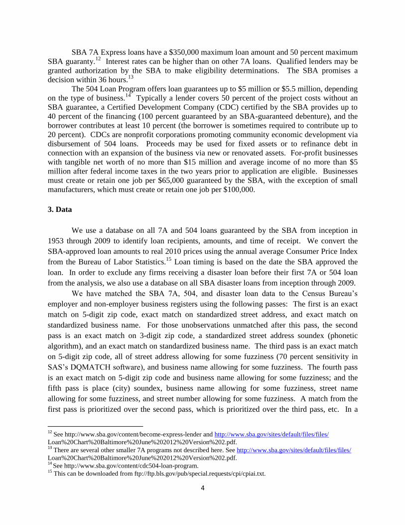
backed loan and of receiving different loan amounts on the number of jobs created. Table 7

therefore contains corresponding results with unlogged employment as dependent variable and

Loan Amount expressed in millions of dollars. The simple DiD result in the first column implies

a gain of 3 jobs from loan receipt, averaged over the whole sample. The other columns again

permit the effect to vary with Loan Amount. Column (2) shows that including Loan Amount

reduces the coefficient on Postloan Dummy to a quarter of its previous magnitude (in column

(1)), statistically insignificantly different from zero, and the magnitude declines still further in

the quadratic specification in column (3) to the tiny value of 0.20. This implies that the

employment gain from loan receipt is associated only with the amount of the loan, not with

selection into the treatment group, evidence that our matching procedures may be working to

reduce selection bias in the estimates. Indeed, in the final quartic specification, in column (4),

the Postloan dummy coefficient is actually negative, which taken literally would imply negative

selection into the SBA loan programs.

The coefficients on Loan Amount imply an increase of 5 in employment associated with

each one million dollars of loans, again with some slight concavity in the relationship between

employment and the size of the loan. As in the analysis of Table 6, this result requires further

examination in the context of possible heterogeneity of loan effects with respect to size and other

firm characteristics. Leaving aside these heterogeneity issues, we can make two rough

calculations of job creation due to SBA loans, in both cases assuming the coefficients in Table 7,

estimated over the period of 1976-2010 can be applied to the “$30 billion in lending support to

60,000 small businesses” in fiscal year 2011. The first uses the specification in column (1) to

multiply the Postloan dummy coefficient of 3.074 increase in employment per loan times the

60,000 small businesses receiving loans to obtain an estimate of 184,440. The second uses

column (2) and multiplies 60,000 by 0.708 (=42,480) and 30 billion*0.0054/1000 (=162,000) for

a total of 204,480. The two estimates are rather close, and although they are significantly less

than the claimed half-million or more “jobs created and retained” by the SBA, they are not in a

different order of magnitude.

The basic identifying assumption in these estimates is that the combination of matching

and regression methods has eliminated unobserved differences in demand for loans by firms that

are correlated with differences in their growth potential. If this assumption is invalid, then it

might be the case that the effects we estimate reflect selection bias in which types of firms are

loan recipients. Note that the inclusion of firm fixed effects in our regressions imply that such a

residual selection bias must be time-varying, and indeed the dynamics results presented above, in

Figure 2, imply that there would have to be a demand shock, a jump in growth potential, exactly

in the loan year and following year. Any other form of selection bias, such as a more rapid trend

growth rate prior to loan receipt, would have been reflected as such in Figure 2.

One way of assessing this potential problem of time-varying demand shocks is to focus

on situations where all firms face a strong increase in demand and thus have good growth

possibilities. For this purpose, we focus on unusually rapid growth environments – cases located

in county-years in the top decile of county-level employment growth rates over the whole

sample; the average employment growth in these cases is 22.2 percent, and the minimum is 11.5

percent – compared with a county-year average of 0.18 percent. We restrict both the treated

firms and controls to come from these unusually high growth situations. If the loan receipt is just

reflecting a greater opportunity for growth among treated firms, then the estimate with this high-

growth-context sample should be zero, or at least attenuated compared to the full sample

estimates in Tables 6 and 7. The results shown in Table 8, however, are rather similar to those

12

for the full data: slightly larger for the coefficient on Postloan in the log(employment) equation,

and slightly smaller in other specifications. The dynamics of the Postloan coefficient in loan-

event time, shown in Figure 3, are also qualitatively similar, with only tiny differences in treated

and control firms prior to loan receipt and large sustained jumps immediately afterward.

Because this sample is smaller, the 99 percent confidence intervals are wider, of course. Overall,

there is no evidence from this analysis that differences in demand conditions drive our results.32

Our methods are designed to estimate the “treatment effect on the treated”(ToT), the

direct effect on firms receiving loans, and they assume the program has no effect on nontreated

firms used as controls in the analysis.33

Because only a tiny fraction of firms in the U.S. receive

SBA-backed loans, this assumption is plausible. But it is nevertheless possible that even if

treated firms grow as a result of loan receipt that the program creates general equilibrium effects,

or spillovers on other firms. The most obvious type of potential spillover would be negative:

displacement effects that reduce employment at nontreated firms that compete with the treated in

product and labor markets. Spillover effects could in principle also be positive, for instance if

the loan enables innovation that is somehow copied or imitated by other firms, and it could also

be positive for firms in upstream or downstream industries from the loan beneficiary. In either

case, the total job creation – including these indirect effects as well as the direct effect – would

differ from the direct effect we have estimated.

Estimating such general equilibrium effects is intrinsically difficult, and it is largely

ignored in the program evaluation literature. Positive spillovers would imply that our estimates

of the direct effect are lower than the total estimate, and therefore we focus attention here on the

possibility of negative displacement effects. If these result from product market competition,

where loan receipt gives the beneficiary an advantage over its competitors, then we should look

for negative effects within industries. If the degree of competition is related to geographic

distance, then we should look for larger negative effects nearer to treated firms than farther

away. In turn, this implies that the estimated ToT should be larger when the controls are drawn

from close by than when they are far away.

To assess this implication, we divide the controls within the kernel bandwidth according

to the distance from treated firm and estimate separately for nearby and far away controls. We

implement this procedure two different ways: in the first, controls are included if they are up to

10 miles away to constitute the “nearby” group, which is compared to a “far away” group more

than 200 miles distant; in the second procedure, we simply take the nearest four controls for the

“nearby” group and the furthest four as “far away.” The displacement hypothesis would predict

that we receive larger estimates for the nearby group than the far away group. Results are shown

in Table 10 and dynamics in Figure 4. In all cases, we find only slightly larger nearby

coefficients implying at most a small amount of displacement – on the order of 1-2 percentage

points of employment effect or 0.1-0.2 jobs from the unlogged specification, on average per loan.

Thus, while the analysis is consistent with displacement, the estimated magnitudes are so small

that they do not support an important role for displacement in driving our results.34

32

An alternative approach would be to consider the control group in rapidly growing contexts as a placebo, or

“pseudo-outcome” group, and to test the difference in their growth compared to controls in less rapidly growing

contexts. We plan to report such tests, which can be implemented in various ways, in future research. 33

The program evaluation literature sometimes refers to this as the “stable unit treatment value assumption”

(SUTVA) (Imbens and Wooldridge 2009). 34

An alternative approach would have been to estimate the difference between the loan impacts on nearby and far-

away controls in a single regression excluding the treated firms, akin to the pseudo-outcome test discussed above.

In fact, based on the linearity of least squares regression, we can infer the results from such an exercise at least

13

The analysis so far assumes no differences in survival rates between treated firms and

controls, although the SBA frequently refers to business survival as a performance measure, and

access to loans may well affect survival. The direction of the effect is not entirely certain,

because while more finance may get a business through hard times, the increased leverage and

possible over-extension may create greater vulnerability. Nor is the measurement of survival

unambiguous, as we can only track firms in the LBD and must classify any disappearance from

the database as an exit. Though great effort has been made to link establishments across time in

the LBD, we cannot always distinguish bankruptcy and other genuine shutdowns from buy-outs

or reorganizations that lead to a change in the identifying code in the LBD. As some of these

outcomes represent business failure, others reflect success, and some level of exit is a normal

feature of a dynamic economy, the analysis of exit is thus also not as clear normatively as our

analysis of employment effects.

With these qualifications in mind, we are nonetheless interested to ascertain the degree to

which our results might be driven by exit effects. Assuming exit represents job loss, then if exit

is more common among loan recipients, then our earlier results are overstated in ignoring the

employment decline associated with exit. On the other hand, if SBA-backed loans raise survival,

then our earlier results could be understated. To distinguish these alternatives, we impute a zero

value for employment in every year following exit and re-estimate the specifications in Table 7

(because zero values are included here, we cannot re-estimate Table 6). The results are slightly

larger but qualitatively similar to those without the imputations, so we conclude that different

patterns of exit are unlikely to play an important role in our results.

Finally, we consider some alternative estimation approaches. Tables 12 and 13 provide

analogous results to Tables 6 and 7 for the logged and unlogged specifications, respectively,

using a 2 percent propensity score bandwidth for the inclusion of controls. The sample is much

smaller, both because there are fewer controls, but also because some treated firms fail to find

controls within the narrower bandwidth that also satisfy the exact year, age, industry, and preloan

size restrictions. The results, however, are qualitatively similar. Figure 5 provides the

corresponding loan dummy dynamics to Figure 2, again with similar implications.

We may consider some approaches that do not use matching or regression, or either.

Table 14 shows mean employment levels pre- and post-treatment for the treated sample and for

all non-treated firms. The latter are about 35 percent smaller compared to post-treatment loan

recipients, but this cannot be interpreted causally because they also differ pre-treatment. If we

consider a matching estimator without regression adjustments, we can calculate the simple

difference-in-differences in the bottom part of Table 14, where treated-control differences are

smaller pre-treatment, and the change is much greater to the post-treatment period. A plot of

these employment levels for the treated and matched controls is shown in Figure 6 for the mean

and in Figure 7 for the median. But without regression adjustment, including fixed effects, there

is still some unobserved heterogeneity reflected in the pre-treatment differences and not

accounted for.

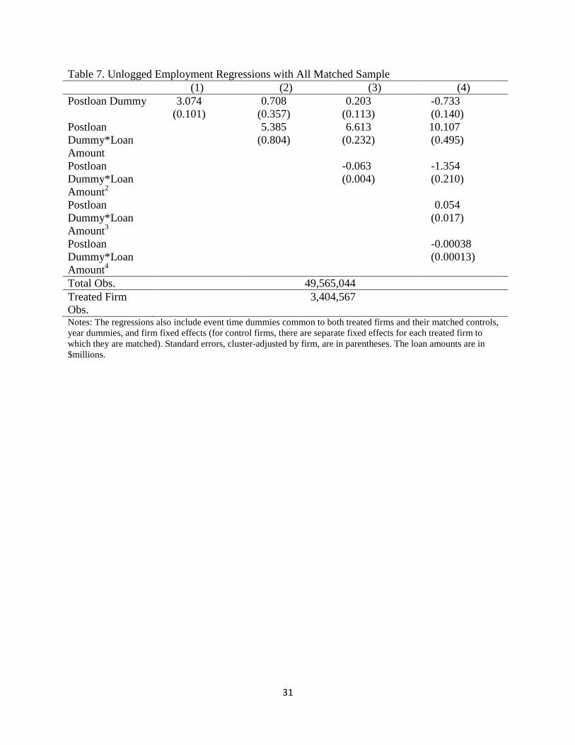
Two other alternative estimators that use regression but not matching include an after-

before estimator using only treated firms, but no control group, and one that includes all non-

roughly from the results in Table 10: assuming identical samples for the nearby and far-away groups (which is

almost exactly satisfied for the nearest 4 versus furthest 4), the coefficient on a nearby dummy variable would be

equal to the difference between the coefficient shown for the far-away group minus the coefficient shown for the

nearby group in the table. For the Postloan dummy specifications, this subtraction gives the magnitudes of

displacement discussed in the text.

14

treated firms as controls. Results for the first of these are shown in Tables 15 and 16. They tend

to imply larger loan effects than those in our preferred specifications using a matched control

group in Tables 6 and 7. For the full-LBD regressions, results are shown in Tables 17 and 18,

the coefficients are still (slightly) larger. We can diagnose potential selection bias in these

specifications by estimating dynamics as before, and the results are shown in Figures 8 and 9 for

these two specifications. Unlike the dynamics from the matched samples, where we observed

only tiny differences between treated and controls in the preloan period, in both Figure 8 and

Figure 9 the differences are substantial and trending strongly upward before the event year.

They also reach higher peaks in the postloan period, but this analysis implies that the results

without matching are plagued by too much selection bias to allow reliable inferences about the

impact of these programs.

6. Conclusion

Our estimates of the effects of the Small Business Administration (SBA) 7(a) and 540

loan programs on employment in this paper are based on an unusual linking of administrative

and census data and an application of econometric methods originally designed for evaluating

labor market training interventions. This approach appears to be fruitful, as we exploit the large

size and completeness of the data to combine matching and regression methods. We match

exactly on firm age, industry, year, and pre-loan size, plus we carry out kernel-based matching

on propensity scores estimated as a function of four years of employment history and other

variables. Having constructed the matched sample, we estimate program effects using firm fixed

effects regressions.

The results can be quickly summarized. We find positive average effects on loan

recipient employment of about 25 percent or 3 jobs at the mean. Including loan amount, we find

little or no impact of loan receipt per se, but an increase of about 5.4 jobs for each million dollars

of loans. Examining loans received only in high growth county-years (average growth of 22

percent), where most small firms should have excellent growth potential, we find similar effects,

implying that the estimates are not driven by differential demand conditions across firms.

Results are also similar regardless of distance of control from recipient firms, suggesting only a

very small role for displacement effects. In all these cases, the results pass a “pre-program”

specification test, where controls and treated firms look similar in the pre-loan period. Other

specifications, such as those using only matching or only regression imply somewhat higher

effects, but they fail the pre-program test.

This paper forms the first part of a much larger project in the area of small business

programs, finance, innovation, and growth. Our focus here is on a single outcome variable,

employment, because job creation has been the central SBA issue and because we can measure

this variable over a longer time period and for more firms than other outcomes we plan to study.

But the results should be treated as preliminary because heterogeneity in firm size and

performance implies that we will likely find considerable heterogeneity in program impacts as

well. There are several important dimensions to this heterogeneity, including firm characteristics

of size, age, location, and industry; program characteristics such as interest rate, term, and SBA

program; and economic environment, including the state of the business cycle. We look forward

to reporting these results in the near future.

References

15

Beck, Thorsten, “The Econometrics of Finance and Growth.” Accessed on March 5, 2011 from

http://www.tilburguniversity.edu/research/institutes-and-research-groups/center/staff/beck/

publications/new/financegrowth.pdf. Forthcoming in Palgrave Handbook of Econometrics,

2011.

Birch, David L., Job Creation in America: How Our Smallest Companies Put the Most People to

Work. New York: Free Press, 1987.

Craig, Ben R., William E. Jackson III, and James B. Thomson, “The Economic Impact of the

Small Business Administration’s Intervention in the Small Firm Credit Market: A Review of the

Research Literature.” Journal of Small Business Management, Vol. 47(2), 221–231, 2009.

Davis, Steven, John Haltiwanger, and Scott Schuh, Job Creation and Destruction. Cambridge,

Mass: The MIT Press, 1996.

Haltiwanger, John, Ron Jarmin, and Javier Miranda, “Who Creates Jobs? Small vs. Large vs.

Young.” Review of Economics and Statistics, forthcoming.

Heckman, James, and Joseph V. Hotz, “Choosing among Alternative Nonexperimental Methods

for Estimating the Impact of Social Programs: The Case of Manpower Training.” Journal of the

American Statistical Association, Vol. 84(408), 862-74, December 1989.

Heckman, James J., Hidehiko Ichimura, and Petra E. Todd, “Matching as an Econometric

Evaluation Estimator: Evidence from Evaluating a Job Training Programme.” Review of

Economic Studies, Vol. 64(4), 605-654, 1997.

Heckman, James J., Hidehiko Ichimura, and Petra E. Todd, “Matching as an Econometric

Evaluation Estimator.” Review of Economic Studies, Vol. 65(2), 261-294, 1998.

Heckman, James J., Robert J. LaLonde, and Jeffrey A. Smith, “The Economics and

Econometrics of Active Labor Market Programs.” In Handbook of Labor Economics, Vol. 3A.

Edited by Orley Ashenfelter and David Card. Elsevier Science B.V., Amsterdam, 1999.

Heckman, James J., Lance Lochner, and Christopher Taber, “Human Capital Formation and

General Equilibrium Treatment Effects: A Study of Tax and Tuition Policy.” Fiscal Studies,

Vol. 20(1), 25-40, 1999.

Hubbard, R. Glenn, “Capital-Market Imperfections and Investment.” Journal of Economic

Literature, Vol XXXVI, 193-225, March 1998.

Imbens, Guido W., and Jeffrey M. Wooldridge, “Recent Developments in the Econometrics of

Program Evaluation,” Journal of Economic Literature, Vol. 47(1), 5-86, 2009.

Jarmin, Ronald S., “Evaluating the Impact of Manufacturing Extension on Productivity Growth.”

Journal of Policy Analysis and Management, Vol. 18(1), 99-119, 1999.

16

Jarmin, Ronald S., and Javier Miranda, “The Longitudinal Business Database.” CES Working

Paper 02-17, 2002.

Levine, Ross, “Finance and Growth: Theory and Evidence.” In Handbook of Economic Growth,

Philippe Aghion and Steven Durlauf (eds.). Netherlands: Elsevier Science, 2005.

Neumark, David, Brandon Wall, and Junfu Zhang, “Do Small Businesses Create More Jobs?

New Evidence for the United States from the National Establishment Time Series.” Review of

Economics and Statistics 93(1), 16-29, 2011.

Parker, Jonathan A., “On Measuring the Effects of Fiscal Policy in Recessions.” NBER

Working Paper No. 17240, 2011.

Parker, Jonathan A., Nicholas S. Souleles, David S. Johnson, and Robert McClelland,

“Consumer Spending and the Economic Stimulus Payments of 2008.” NBER Working Paper

No. 16684, 2011.

Ramey, Valerie A., “Identifying Government Spending Shocks: It’s all in the Timing.” Quarterly

Journal of Economics, Vol. 126(1), 1-50, 2011.

Rosenbaum, P., and D. B. Rubin, “Constructing a Control Group Using a Multivariate Matched

Sampling Method that Incorporates the Propensity Score.” The American Statistician, Vol. 39,

pp. 33-38, 1985.

Stiglitz, Joseph, and Andrew Weiss, “Credit Rationing in Markets with Imperfect Information.”

American Economic Review, Vol. 71, 393-410, 1981.

ftp://ftp.bls.gov/pub/special.requests/cpi/cpiai.txt

http://www.census.gov/geo/www/gazetteer/gazette.html

http://www.sba.gov/about-sba-info/11572

http://www.sba.gov/content/become-express-lender

http://www.sba.gov/content/standard-7a-evaluation-criteria

http://www.sba.gov/content/steps-participating-clp

http://www.sba.gov/content/steps-participating-plp

http://www.sba.gov/content/7a-terms-conditions

http://www.sba.gov/sites/default/files/SBA%20FORM%202301%20B.pdf

http://www.sba.gov/sites/default/files/files/Loan%20Chart%20Baltimore%20June%202012%20Version

%202.pdf

17

http://www.sba.gov/sites/default/files/files/1-

508%20Compliant%20FY%202013%20CBJ%20FY%202011%20APR%281%29.pdf

http://www.sba.gov/sites/default/files/files/2-

508%20Compliant%20Appendix%20FY%202012%20CBJ%20FY%202011%20APR%281%29.

pdf

http://www.sba.gov/sites/default/files/files/Size_Standards_Table.pdf

Whitehouse.gov, “Weekly Address: President Obama Calls for New Steps to Support America’s

Small Businesses,” February 6, 2010.

18

Figure 1. Number of SBA Loans and Loan Amount by Year

0

5000

10000

15000

20000

25000

30000

35000

0

20000

40000

60000

80000

100000

120000

19

77

19

79

19

81

19

83

19

85

19

87

19

89

19

91

19

93

19

95

19

97

19

99

20

01

20

03

20

05

20

07

20

09

Loan

Am

ou

nt

($M

illio

ns)

Nu

mb

er

of

Loan

s

Number of Loans Loan Amount ($Millions)

19

Figure 2. Loan Dummy Dynamics, All Matched Sample

-0.05

0

0.05

0.1

0.15

0.2

0.25

0.3

0.35

-4 -3 -2 -1 0 1 2 3 4 5 6 7 8 9 10+

Years Before/After Loan

20

Figure 3. Loan Dummy Dynamics, Growing Counties Matched Sample

-0.2

-0.1

0

0.1

0.2

0.3

0.4

0.5

0.6

-4 -3 -2 -1 0 1 2 3 4 5 6 7 8 9 10+

Years Before/After Loan

21

Figure 4. Loan Dummy Dynamics, Matched Samples by Treated-Control Distance

-0.05

0

0.05

0.1

0.15

0.2

0.25

0.3

-4 -3 -2 -1 0 1 2 3 4 5 6 7 8 9 10+

Years Before/After Loan

<=10 Miles >200 miles Nearest 4 Furthest 4

22

Figure 5. Loan Dummy Dynamics, Matched Sample With +/- 2 Percent Propensity Score

Bandwidth

-0.1

-0.05

0

0.05

0.1

0.15

0.2

0.25

0.3

0.35

0.4

-4 -3 -2 -1 0 1 2 3 4 5 6 7 8 9 10+

Years Before/After Loan

23

Figure 6. Mean Firm Employment by Year Before/After Loan

0

5

10

15

20

25

30

35

-4 -3 -2 -1 0 1 2 3 4 5 6 7 8 9 10+

Years Before/After Loan

treated firms matched non-treated firms

24

Figure 7. Median Firm Employment by Year Before/After Loan

0

2

4

6

8

10

12

14

-4 -3 -2 -1 0 1 2 3 4 5 6 7 8 9 10+

Years Before/After Loan

treated firms matched non-treated firms

25

Figure 8. Loan Dummy Dynamics, Regressions with Treated Firms Only

0

0.1

0.2

0.3

0.4

0.5

0.6

0.7

0.8

-4 -3 -2 -1 0 1 2 3 4 5 6 7 8 9 10+

Years Before/After Loan

26

Figure 9. Loan Dynamics, All LBD

0

0.1

0.2

0.3

0.4

0.5

0.6

0.7

-4 -3 -2 -1 0 1 2 3 4 5 6 7 8 9 10+

Years Before/After Loan

27

Table 1. Path from Full SBA Loan Dataset to All Matched Regression Sample

Number

Total SBA Loans in 1977-2009 1,378,501

Except loans not matched to any business register 763,583

Except loans matched to non-employer business register 604,023

Except recipients receiving first SBA 7A/504 loan before 1977 or a

SBA disaster loan before its first SBA 7A/504 loan

528,753

Except SBA 7A/504 loans after the first loan 493,116

Except start-ups 337,148

Except multi-establishment firms 318,207

Except firms with missing employment in year before loan receipt 269,623

Except firms without controls (main regression sample) 216,023

Table 2. Sample Comparisons

Not Matched to

Any Business

Register, Non-

Start-Up

According to

SBA

Not in

Regressions

Because

Missing

Employment in

Year Before

Loan

Not in

Regressions

Because No

Control Firms

Found

In Regressions

Total Number 398,088 48,584 53,600 216,023

Mean Employment 11.87 8.86 16.73 14.80

Percent Sole

Proprietorships

39.09 20.02 13.47 18.74

Percent Partnerships 5.35 4.10 3.33 3.49

Percent Minority 28.00 22.96 13.51 21.29

Percent Female 27.59 27.68 22.25 26.17

Percent Veteran 11.23 10.83 13.79 11.47

Percent By Sector:

Construction 6.39 9.40 5.73 9.19

Manufacturing 5.50 6.22 14.36 7.16

Wholesale Trade 4.70 4.93 6.38 5.39

Retail Trade 12.90 11.08 10.33 11.66

Finance/Insurance/

Real Estate

2.69 2.51 1.37 2.36

Services 33.89 29.98 17.52 31.18

Other/Unknown 33.93 35.88 44.31 33.06 Notes: The variables come from the SBA loan recipient database.

28

Table 3. Descriptive Statistics

All Non-Treated Firms All Treated Firms

Employment Mean 12.54 12.46

Employment Standard

Deviation

129.70 26.91

Employment Median 4 6

Age Mean 8.20 6.74

Age Standard Deviation 7.61 6.59

Age Median 6 4

Percent by Sector:

Construction 11.15% 10.80%

Manufacturing 5.36% 12.62%

Wholesale Trade 6.21% 10.83%

Retail Trade 8.22% 12.58%

Finance/Insurance/Real

Estate

2.55% 1.87%

Services 55.47% 44.93%

Other 11.05% 6.37% Notes: This excludes multi-establishment firms and establishments that were ever in a multi-establishment firm in

the past. Non-treated firms are included in each year they appear in the LBD, while treated firms are included only

in the treatment year. For treated firms, employment is measured in the year prior to treatment. The variables come

from the LBD.

Table 4. Number of Firms and Firm-Year Observations in Regressions with All Matches

Number of

Firms

Pre-Treatment

Firm-Years

Pre-Treatment

Years/Firm

Post-

Treatment

Firm-Years

Post-

Treatment

Years/Firm

Treated 216,023 2,051,524 9.5 1,353,043 6.3

Controls 3,508,245 30,404,010 8.7 15,756,467 4.5 Notes: The year of loan receipt is counted as a pre-treatment year here.

29

Table 5. Bias Before and After Propensity Score Matching

Variable Mean

All Non-

Treated

All Treated Treated in

Regression

Sample

Controls in

Regression

Sample

% Bias in

Regression

Sample

% Bias

Reduction

Log Emp t-

1

1.307 1.702 1.847 1.879 -2.473 92.050

Log Emp t-

1 sq.

3.455 4.374 4.696 4.791 -1.781 89.739

Log Emp t-

1 – t-2

0.107 0.229 0.228 0.220 1.198 93.708

Log Emp t-

2 – t-3

0.095 0.186 0.198 0.192 0.909 94.176

Log Emp t-

3 – t-4

0.082 0.151 0.164 0.162 0.449 96.474

Log Wage 2.151 2.625 2.963 2.985 -1.641 95.297

Age 7.496 7.160 8.030 8.239 -2.928 37.624 Notes: % bias is the standardized difference, which for a given variable, say age, is

( )

∑ [ ∑ ( ) ]

√ ( ) ( )

. The all non-treated group is included in all years they appear in the

LBD. The other three groups are included only in the treatment year.

30

Table 6. Log Employment Regressions with All Matched Sample

(1) (2) (3) (4)

Postloan Dummy 0.241

(0.002)

0.228

(0.002)

0.241

(0.003)

0.244

(0.003)

Postloan

Dummy*Log

Loan Amount

0.070

(0.002)

0.071

(0.002)

0.064

(0.003)

Postloan

Dummy*Log

Loan Amount2

-0.0084

(0.0010)

-0.0108

(0.0011)

Postloan

Dummy*Log

Loan Amount3

0.00192

(0.00062)

Postloan

Dummy*Log

Loan Amount4

0.000220

(0.000057)

Total Obs. 49,565,044

Treated Firm

Obs.

3,404,567

Notes: The regressions also include event time dummies common to both treated firms and their matched controls,

year dummies, and firm fixed effects (for control firms, there are separate fixed effects for each treated firm to

which they are matched). Standard errors, cluster-adjusted by firm, are in parentheses. The log loan amount is the

difference between the firm’s log loan amount and the mean of the log loan amount among treated firms in the

sample.

31

Table 7. Unlogged Employment Regressions with All Matched Sample

(1) (2) (3) (4)

Postloan Dummy 3.074

(0.101)

0.708

(0.357)

0.203

(0.113)

-0.733

(0.140)

Postloan

Dummy*Loan

Amount

5.385

(0.804)

6.613

(0.232)

10.107

(0.495)

Postloan

Dummy*Loan

Amount2

-0.063

(0.004)

-1.354

(0.210)

Postloan

Dummy*Loan

Amount3

0.054

(0.017)

Postloan

Dummy*Loan

Amount4

-0.00038

(0.00013)

Total Obs. 49,565,044

Treated Firm

Obs.

3,404,567

Notes: The regressions also include event time dummies common to both treated firms and their matched controls,

year dummies, and firm fixed effects (for control firms, there are separate fixed effects for each treated firm to

which they are matched). Standard errors, cluster-adjusted by firm, are in parentheses. The loan amounts are in

$millions.

32

Table 8. Log Employment Regressions with Growing Counties Matched Sample

(1) (2)

Postloan Dummy 0.263

(0.026)

0.257

(0.025)

Postloan Dummy*Log

Loan Amount

0.054

(0.019)

Total Obs. 1,017,275

Treated Firm Obs. 21,171 Notes: The regressions also include event time dummies common to both treated firms and their matched controls,

year dummies, and firm fixed effects (for control firms, there are separate fixed effects for each treated firm to

which they are matched). Standard errors, cluster-adjusted by firm, are in parentheses. The log loan amount is the

difference between the firm’s log loan amount and the mean of the log loan amount among treated firms in the

sample. Treated and control firms are included in this sample only if they are located in counties with total

employment growth between the year before the treated firm’s loan receipt and the year of loan receipt that is in the

top decile of employment growth (10.9 percent) among county-year observations in the LBD. Geography is not used

for exact matching among treated and control firms in this sample.

Table 9. Unlogged Employment Regressions with Growing Counties Matched Sample

(1) (2)

Postloan Dummy 2.338

(0.510)

0.540

(0.448)

Postloan Dummy*Loan

Amount

4.360

(0.740)

Total Obs. 1,017,275

Treated Firm Obs. 21,171 Notes: The regressions also include event time dummies common to both treated firms and their matched controls,

year dummies, and firm fixed effects (for control firms, there are separate fixed effects for each treated firm to

which they are matched). Standard errors, cluster-adjusted by firm, are in parentheses. The loan amounts are in

$millions. Treated and control firms are included in this sample only if they are located in counties with total

employment growth between the year before the treated firm’s loan receipt and the year of loan receipt that is in the

top decile of employment growth (10.9 percent) among county-year observations in the LBD. Geography is not used

for exact matching among treated and control firms in this sample.

33

Table 10. Regressions with Control Groups by Geographic Distance from Matched Treated

Firms

<=10 miles >200 miles Nearest 4 Furthest 4

Log Employment

Postloan Dummy 0.199

(0.007)

0.180

(0.006)

0.203

(0.004)

0.194

(0.004)

Postloan Dummy 0.187

(0.007)

0.168

(0.007)

0.191

(0.004)

0.181

(0.004)

Postloan

Dummy*Log Loan

Amount

0.064

(0.004)

0.062

(0.004)

0.061

(0.002)

0.061

(0.002)

Postloan Dummy 0.191

(0.008)

0.171

(0.008)

0.198

(0.005)

0.189

(0.005)

Postloan

Dummy*Log Loan

Amount

0.065

(0.004)

0.063

(0.004)

0.062

(0.002)

0.062

(0.002)

Postloan

Dummy*Log Loan

Amount2

-0.0020

(0.0026)

-0.0018

(0.0026)

-0.0045

(0.0016)

-0.0045

(0.0016)

Unlogged Employment

Postloan Dummy 1.603

(0.138)

1.481

(0.110)

2.277

(0.134)

2.143

(0.145)

Postloan Dummy 0.461

(0.143)

0.348

(0.119)

0.444

(0.166)

0.315

(0.175)

PostloanDummy*

Loan Amount

3.388

(0.333)

3.360

(0.333)

4.540

(0.221)

4.533

(0.221)

Postloan Dummy 0.134

(0.138)

0.029

(0.115)

-0.001

(0.182)

-0.128

(0.190)

Postloan Dummy*

Loan Amount

4.898

(0.455)

4.831

(0.452)

6.143

(0.320)

6.131

(0.320)

Postloan Dummy*

Loan Amount2

-0.502

(0.120)

-0.489

(0.119)

-0.405

(0.052)

-0.404

(0.052)

Total Obs. 1,352,061 4,237,998 4,961,474 4,942,141

Treated Firm Obs. 371,925 371,925 1,079,342 1,079,993 Notes: The regressions also include event time dummies common to both treated firms and their matched controls,

year dummies, and firm fixed effects (for control firms, there are separate fixed effects for each treated firm to

which they are matched). Standard errors, cluster-adjusted by firm, are in parentheses. The log loan amount is the

difference between the firm’s log loan amount and the mean of the log loan amount among treated firms in the

sample. The loan amounts are in $millions. The first and second control group is non-treated firms located no more

than 10 miles away and more than 200 miles away from the treated firms to which they are matched, respectively.

Only treated firms that have controls in both control groups are included in the regressions. The third and fourth

control groups are the nearest and furthest four firms from the treated firms to which they are matched. Only treated

firms that have at least eight control firms are included in the regressions.

34

Table 11. Unlogged Employment Regressions with Matched Sample,

Imputing Zero Employment After Exit

(1) (2) (3) (4)

Postloan Dummy 3.258

(0.075)

2.215

(0.239)

1.891

(0.083)

1.774

(0.095)

Postloan Dummy*Loan

Amount

2.470

(0.560)

3.278

(0.186)

3.709

(0.330)

Postloan Dummy*Loan

Amount2

-0.030

(0.002)

-0.179

(0.117)

Postloan Dummy*Loan

Amount3

0.0039

(0.0059)

Postloan Dummy*Loan

Amount4

-0.000023

(0.000044)

Total Obs. 77,118,506

Treated Firm Obs. 4,526,915 Notes: The regressions also include event time dummies common to both treated firms and their matched controls,

year dummies, and firm fixed effects (for control firms, there are separate fixed effects for each treated firm to

which they are matched). Standard errors are cluster-adjusted by firm. The loan amount is in $millions. Zero

employment is imputed in all years after exit (i.e., through 2010).

Table 12. Log Employment Regressions with Sample Matched by +/-2 Percent Bandwidth

(1) (2) (3) (4)

Postloan Dummy 0.226

(0.003)

0.212

(0.003)

0.223

(0.004)

0.236

(0.004)

Postloan

Dummy*Log

Loan Amount

0.067

(0.002)

0.068

(0.002)

0.063

(0.003)

Postloan

Dummy*Log

Loan Amount2

-0.0067

(0.0012)

-0.0230

(0.0030)

Postloan

Dummy*Log

Loan Amount3

0.00148

(0.00067)

Postloan

Dummy*Log

Loan Amount4

0.00022

(0.00004)

Total Obs. 12,623,202

Treated Firm Obs. 2,379,029 Notes: The regressions also include event time dummies common to both treated firms and their matched controls,

year dummies, and firm fixed effects (for control firms, there are separate fixed effects for each treated firm to

which they are matched). Standard errors, cluster-adjusted by firm, are in parentheses. The log loan amount is the

difference between the firm’s log loan amount and the mean of the log loan amount among treated firms in the

sample.

35

Table 13. Unlogged Employment Regressions with Sample Matched by +/-2 Percent Bandwidth

(1) (2) (3) (4)

Postloan Dummy 2.998

(0.126)

0.448

(0.142)

-0.187

(0.163)

-0.951

(0.165)

Postloan Dummy

*Loan Amount

5.814

(0.265)

7.860

(0.428)

11.379

(0.535)

Postloan Dummy

*Loan Amount2

-0.482

(0.088)

-2.398

(0.226)

Postloan Dummy

*Loan Amount3

0.186

(0.025)

Postloan Dummy

*Loan Amount4

-0.0042

(0.0007)

Total Obs. 12,623,202

Treated Firm Obs. 2,379,029 Notes: The regressions also include event time dummies common to both treated firms and their matched controls,

year dummies, and firm fixed effects (for control firms, there are separate fixed effects for each treated firm to

which they are matched). Standard errors, cluster-adjusted by firm, are in parentheses. The loan amounts are in

$millions.

Table 14. Mean Employment With and Without Matching

Pre-Treatment Post-Treatment

Without Matching:

Treated 11.91 20.90

Non-Treated 15.69

With Matching:

Treated 10.84 20.17

Non-Treated 12.44 18.96 Notes: The year of loan receipt is included as a pre-treatment year. The post-treatment years for non-treated firms

with matching are the post-treatment years of the treated firms to which the non-treated firms are matched.

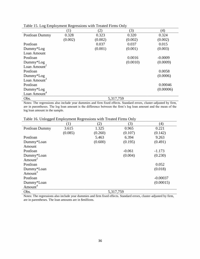
36

Table 15. Log Employment Regressions with Treated Firms Only

(1) (2) (3) (4)

Postloan Dummy 0.328

(0.002)

0.323

(0.002)

0.320

(0.002)

0.324

(0.002)

Postloan

Dummy*Log

Loan Amount

0.037

(0.001)

0.037

(0.001)

0.015

(0.003)

Postloan

Dummy*Log

Loan Amount2

0.0016

(0.0010)

-0.0009

(0.0009)

Postloan

Dummy*Log

Loan Amount3

0.0058

(0.0006)

Postloan

Dummy*Log

Loan Amount4

0.00046

(0.00006)

Obs. 5,317,759 Notes: The regressions also include year dummies and firm fixed effects. Standard errors, cluster-adjusted by firm,

are in parentheses. The log loan amount is the difference between the firm’s log loan amount and the mean of the

log loan amount in the sample.

Table 16. Unlogged Employment Regressions with Treated Firms Only

(1) (2) (3) (4)

Postloan Dummy 3.615

(0.085)

1.325

(0.260)

0.965

(0.107)

0.221

(0.142)

Postloan

Dummy*Loan

Amount

5.463

(0.600)

6.394

(0.195)

9.263

(0.491)

Postloan

Dummy*Loan

Amount2

-0.061

(0.004)

-1.173

(0.230)

Postloan

Dummy*Loan

Amount3

0.052

(0.018)

Postloan

Dummy*Loan

Amount4

-0.00037

(0.00015)

Obs. 5,317,759 Notes: The regressions also include year dummies and firm fixed effects. Standard errors, cluster-adjusted by firm,

are in parentheses. The loan amounts are in $millions.

37

Table 17. Log Employment Regressions with All LBD Sample

(1) (2) (3) (4)

Postloan Dummy 0.340

(0.088)

0.328

(0.002)

0.340

(0.002)

0.343

(0.002)

Postloan

Dummy*Log

Loan Amount

0.056

(0.001)

0.056

(0.001)

0.044

(0.002)

Postloan

Dummy*Log

Loan Amount2

-0.0075

(0.0008)

-0.0103

(0.0009)

Postloan

Dummy*Log

Loan Amount3

0.0033

(0.0005)

Postloan

Dummy*Log

Loan Amount4

0.00034

(0.00006)

Total Obs. 250,117,749

Treated Firm

Obs.

5,317,759

Notes: The regressions also include year dummies and firm fixed effects. Standard errors, cluster-adjusted by firm,

are in parentheses. The log loan amount is the difference between the firm’s log loan amount and the mean of the

log loan amount among treated firms in the sample.

Table 18. Unlogged Employment Regressions with All LBD Sample

(1) (2) (3) (4)

Postloan Dummy 3.648

(0.088)

1.197

(0.271)

0.814

(0.096)

-0.050

(0.132)

Postloan

Dummy*Loan

Amount

5.526

(0.604)

6.469

(0.197)

9.713

(0.515)

Postloan

Dummy*Loan

Amount2

-0.062

(0.004)

-1.329

(0.246)

Postloan

Dummy*Loan

Amount3

0.060

(0.020)

Postloan

Dummy*Loan

Amount4

-0.00043

(0.00016)

Total Obs. 250,117,749

Treated Firm

Obs.

5,317,759

Notes: The regressions also include year dummies and firm fixed effects. Standard errors, cluster-adjusted by firm,

are in parentheses. The loan amounts are in $millions.