WP/14/24

Do Forecasters Believe in Okun’s Law? An Assessment of Unemployment and Output

Forecasts

Laurence Ball, João Tovar Jalles, and Prakash Loungani

© 2014 International Monetary Fund WP/14/24

IMF Working Paper

Research Department

Do Forecasters Believe in Okun’s Law? An Assessment of Unemployment and Output Forecasts

Prepared by Laurence Ball, João Tovar Jalles, and Prakash Loungani1

Authorized for distribution by Prakash Loungani

February 2014

Abstract

This paper provides an assessment of the consistency of unemployment and output forecasts. We show that, consistent with Okun’s Law, forecasts of real GDP growth and the change in unemployment are negatively correlated. The Okun coefficient—the responsiveness of unemployment to growth—from forecasts is fairly similar to that in the data for various countries. Furthermore, revisions to unemployment forecasts are negatively correlated with revisions to real GDP forecasts. These results are based on forecasts taken from Consensus Economics for nine advanced countries since 1989.

JEL Classification Numbers: C53, E27, E37, E62, D8

Keywords: Unemployment; forecast revisions; Okun’s Law; Great Recession; forecast assessment

Author’s E-Mail Addresses: lball@jhu.edu; jjalles@imf.org; ploungani@imf.org

1 Johns Hopkins University and International Monetary Fund, respectively. The authors are grateful to Hites Ahir, Angela Espiritu and Ezgi Ozturk for excellent research assistance. We also thank Amy Guisinger for valuable help and comments on previous drafts of this paper.

This Working Paper should not be reported as representing the views of the IMF. The views expressed in this Working Paper are those of the author(s) and do not necessarily represent those of the IMF or IMF policy. Working Papers describe research in progress by the author(s) and are published to elicit comments and to further debate.

2

Contents Page

I. Introduction ............................................................................................................................3 

II. Estimating Okun’s Law with Forecasts ................................................................................4 A. Structure of Forecast Data.........................................................................................4 B. Estimating Okun’s Law .............................................................................................5 

III. Okun’s Law: Data vs. Forecasts ..........................................................................................6 

IV. Evidence from Forecast Revisions ......................................................................................9 

V. Conclusions .........................................................................................................................12  References…………………………………………………………………………………… 17 Tables

1. Okun’s Coefficients Comparison: Data vs. Forecasts……………... ………………………7 2. Unemployment Rate and GDP Growth Forecast Revisions……………...………………. 10 Figures

1. Okun’s Coefficients Comparison: Actual vs. Forecast Data………………………………. 8 2. Unemployment Rate and GDP Growth Forecast Revisions……………...………………..11 Appendix…………………………………………………………………………………….. 13 Appendix Tables

3. Okun's Law: Current Year Forecasts……………...……………………………………… ..13 4: Okun's Law: Year-Ahead Forecasts…………...................................................................... 14 Appendix Figures

3. Distributions of Actual and Forecasted Unemployment Rate and GDP Growth: Consensus 1989-2012……………...……………………………………………………….15 4. Unemployment Rate and GDP Growth Forecast Errors: Consensus 1989-2012………......16

3

I. INTRODUCTION

Okun (1962) reported a negative short-run correlation between unemployment and output that has become known as Okun’s Law and is a staple of macroeconomic textbooks. Blanchard and Fischer (1989) include it in their chapter on useful models in Lectures on Macroeconomics. Blinder (1997) refers to it as a “truly sturdy empirical regularity” that constitutes part of “the core of practical macroeconomics that we should all believe”. Leading textbooks such as Mankiw (2012) and Romer (2012) feature Okun’s Law as an empirical regularity.

This paper studies whether economic forecasters share this strong belief in the validity of Okun’s Law. As Mitchell and Pierce (2010) state, “if stable empirical relationships exist among macroeconomic variables, we should expect the public forecasts of professional economic forecasters to be generally consistent with these relationships.” In this respect, this paper contributes to the literature on whether forecasters’ beliefs are consistent with other commonly-used macroeconomics relationships such as the Phillips Curve and the Taylor Rule.2

Our work is also related to recent work on multivariate assessment of forecasts. Sinclair, Stekler and Carnow (2014) note that forecast evaluation methods have traditionally examined forecasts of individual variables. However, as they argue, forecasts are “often relied upon to provide a holistic picture of the state of the economy. In that case the forecasts of all important variables should be evaluated jointly in a multivariate framework.” They suggest several methods of joint evaluation of forecasts of several variables and provide an application to the case of U.S. forecasts of real growth, inflation and unemployment.

The source of the data used in this paper is Consensus Economics. We restrict attention to a group of advanced economies—the G7 economies plus Australia and New Zealand—for which forecasts are available for a long enough time span that we can reliably estimate whether Okun’s Law holds. The time period covered is 1989 to 2012.

Two recent papers have looked at forecasters’ belief in Okun’s Law. Mitchell and Pearce (2010) used forecasts only for the United States and a different data source, viz. the Wall Street Journal’s semi-annual survey, from the one we use. They found that “predictions of unemployment and real growth move in opposite directions, as per Okun’s Law.” For the period 1999 to 2007, the Okun coefficient—the responsiveness of unemployment changes to GDP growth—is about -0.6 in the data and about -0.75 in the forecasts.

The second paper is by Pierdzioch, Rülke and Stadtmann (2011). They use the same data source as in this paper, roughly the same set of countries (the G7), and a sample period from 1989 to 2007. One difference between their work and ours is that they use individual-level forecasts, whereas we use the mean of the individual forecasts, the so-called “consensus”. Setting aside this difference, our work makes three contributions that bolster their finding that forecasters believe

2 Fendel, Lis and Rülke (2011) provide evidence, using data from the same source as the one used in this paper, that unemployment and inflation forecasts for G7 countries are consistent with a belief in the Phillips curve. Mitchell and Pearce (2010) find that interest rates “responded more in accord with the Taylor Rule than is evident in the predictions” of United States forecasters.

4

in Okun’s Law. First, we provide a comparison of how the estimated Okun’s Law based on forecasts matches up with that in the data, drawing on the recent work of Ball, Leigh and Loungani (2013). Second, we exploit the availability of repeated revisions of the forecasts to show that revisions in unemployment forecasts are related to revisions of real GDP forecasts in a manner consistent with Okun’s Law. Third, the five years that we add to their sample period are the momentous ones of the Great Recession during which both Okun’s Law and forecasters belief in it were subjected to a severe test.3

The remainder of the paper is organized as follows. Section II describes the structure of forecasts on unemployment and real GDP and our procedure for estimating Okun’s Law using these forecasts. In Section III we compare estimates of the Okun’s coefficient from forecasts to those in the data. Section IV presents evidence on the relationship between forecast revisions in unemployment and output. Conclusions are in Section V.

II. ESTIMATING OKUN’S LAW WITH FORECASTS

A. Structure of Forecast Data

The forecasts we use have been published on a monthly basis by Consensus Economics, Inc. since October 1989 for major advanced economies. For each country there are between 10 and 30 forecasters. As noted, we use the arithmetic mean of these forecasts, the consensus. The countries consist of the G7 plus Australia and New Zealand, which are the set of countries for which a long time series of forecasts is available. In addition to consensus forecasts, our data set includes (actual) real GDP growth and unemployment rates from the IMF’s International Financial Statistics.4

The events being forecasted are year-over-year real GDP growth and the annual average unemployment rate. Every month a new forecast is made of each event and for two target years, the current year and the year ahead. Hence, for each target year, we have a sequence of 24 forecasts; we index this sequence by h (for horizon), with h=24 denoting forecasts made in January of the year ahead and h=1 denoting forecasts made in December of the current year. We refer to forecasts made in the same year as the target year (h=1 to 12) as current-year forecasts and those made in the year before the target year (h=13 to 24) as year-ahead forecasts. The basic properties of the data and forecasts are discussed in the Appendix. The forecasts display the reasonable property that the frequency distribution of forecasts starts to mirror the frequency distribution of the data as the forecast horizon draws to a close. Moreover, the magnitude of the

3 Tillmann (2010) finds that “individual forecasts for output growth and unemployment submitted by FOMC members suggest that the link between these two variables weakened significantly” in the 1990s, which he suggests arose because “policymakers were aware of a change in labor productivity” over this period. 4 It may be preferable to use the early releases of the unemployment and GDP data (since it is likely that these are closer to the objects that forecasters are trying to predict) rather than the final revised data. In practice, however, the choice of the early release (or ‘real time’) data vs. final data does not make a big difference, as Guisinger and Sinclair (2014) show in their comment on this paper. Similarly, Pierdzioch and others find that estimates of the Okun’s Law for the U.S. are similar whether one uses the final data or the real time data from the Federal Reserve Bank of Philadelphia database.

5

forecast errors declines with horizon.5

B. Estimating Okun’s Law

Okun’s Law is generally written as:

Ut – Ut* = β (Yt – Yt

*) + εt β < 0 ( 1 )

where Ut is the unemployment rate, Yt is the log of output and the * indicates a long-run level. As Ball and others (2013) discuss, the magnitude of the Okun coefficient “is difficult to pin down a priori. It depends on the costs of adjusting employment, which include both technological costs such as training and costs created by employment protection laws. The coefficient also depends on the number of workers who are marginally attached to the labor force, entering and exiting as employment fluctuates.” Since these factors differ across countries, it is quite likely that the Okun coefficient will also differ across countries.

In addition to the “levels” or “gap” version shown in equation (1), there is a “changes” version of Okun’s Law:

ΔUt = α + β ΔYt + ωt ( 2 )

where Δ is the change from the previous period. This equation follows from equation (1) if the natural rate U* is assumed to be constant and potential output Y* is assumed to grow at a constant rate. In this case, differencing equation (1) yields equation (2) with α = –β ΔY *, where ΔY * is the constant growth rate of potential output, and ωt = Δ εt.

In principle, it is better to estimate equation (1) because the implicit assumptions of a constant natural rate of unemployment and constant long-run growth rate of output may not always be reasonable. In this paper, however, we rely on estimates of equation (2). The reason is that otherwise—when we compare estimates of Okun’s Law in the data with that in the forecasts—we would need to know the forecasters’ estimates of U* and Y*, which we do not have. In any case, as Ball and others (2013) note, at least in the data both equations (1) and (2) fit quite well for most advanced countries.

We estimate the following version of equation (2) using forecasts:

Eh ΔUt = α + β Eh ΔYt ( 3 )

where Eh ΔUt and Eh ΔYt are the forecasts made at horizon h of the change in unemployment and

5 Both unemployment and real GDP forecasts show negative bias (that is, forecasts over-estimate both unemployment and real GDP growth). Moreover the bias in unemployment declines from h=24 to h=10 and then increases; while this pattern is difficult to explain, the magnitude of the bias is quite small. Explaining these biases is not the focus of the paper and they do not affect the reliability of the main results.

6

real GDP growth. As noted earlier, h varies from 1 to 24. In the empirical work we will report regression results for various choices of h. Obtaining Eh ΔYt is easy since we directly have forecasts of real GDP growth. Computing Eh ΔUt is a bit more complicated because forecasters predict levels of unemployment in the current and following year, rather than changes. We compute forecasted changes, Eh ΔUt, in slightly different ways for different horizons h. For h<=12, which are forecasts made during year t, we compute Eh

ΔUt as the forecast of unemployment in t minus actual unemployment in year t-1. For example, E6 ΔU1990 is the July 1990 forecast of unemployment in 1990 minus actual unemployment in 1989. For h>12, which are forecasts made during year t-1, we compute Eh ΔUt from forecasts of unemployment in both t and t-1. For example, E18 ΔU1990 is the difference between forecasts for unemployment in 1990 and 1989, both made in July 1989.

III. OKUN’S LAW: DATA VS. FORECASTS

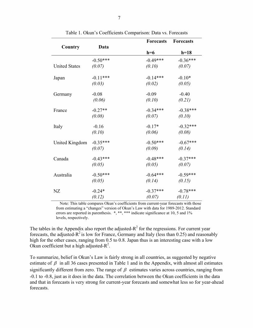
How does the Okun coefficient from the forecasts compare with that in the data? To answer this question, we estimate Okun’s Law using unemployment changes and real GDP growth using annual data from 1989 to 2012.6 In the main text of the paper, we compare these estimates to those from forecasts for two choices of horizon, h = 6 and h = 18.

As shown in Table 1, the estimate of , the Okun coefficient, is negative for all nine countries. It is significantly different from zero in all cases except that of Germany and Italy. Our key finding in this section is that forecasts indicate a belief in Okun’s Law. For the case of h = 6, for example, all estimates of the Okun coefficient are negative and significantly different from zero, except for Germany. There are three cases where the coefficient is low in absolute magnitude: Germany, Italy and Japan, where the range is -0.1 to -0.2. For the other six cases, the range is -0.34 to -0.64. It is evident from Table 1 that, for the case of h = 6, estimates of the Okun coefficient from the data line up very closely with that from the forecasts. Countries with low Okun’s coefficients in the data—Germany, Italy and Japan—are also the ones with low coefficients with forecasts, while Australia has the highest coefficient in both cases. The correlation coefficient between the two sets of estimates is 0.95. The results in Table 1 also show that using a different forecast horizon such as h = 18 does not make a big difference to the results. In the Appendix, we report results for two other forecast horizons, h=9 and 21. In all cases the estimate of the Okun coefficient is negative and in the vast majority of cases it is significantly different from zero. For h=9, the results are virtually identical to those reported for h = 6 in Table 1 above; the correlation between the Okun’s coefficient from the data and that from forecasts remains high at 0.95. In the case of the year-ahead forecasts, this correlation drops to 0.33 for h=18 and 0.45 for h=21. In both cases, however, the correlation is influenced by two outliers, Germany and New Zealand; without these two the correlation rises to 0.62 (for h=18) and 0.71 (for h=21).

6 Ball and others (2013) report estimates of the “gap” version of Okun’s Law for 20 advanced economies, including the nine studied in this paper, for the period 1980 to 2011.

7

Table 1. Okun’s Coefficients Comparison: Data vs. Forecasts

Forecasts Forecasts Country

Data

h=6 h=18

-0.50***

-0.49***

-0.36*** United States (0.07) (0.10) (0.07)

Japan

-0.11***

-0.14***

-0.10* (0.03) (0.02) (0.05)

Germany

-0.08

-0.09

-0.40 (0.06) (0.10) (0.21)

France

-0.27**

-0.34***

-0.38*** (0.08) (0.07) (0.10)

Italy

-0.16

-0.17*

-0.32*** (0.10) (0.06) (0.08)

United Kingdom

-0.35***

-0.50***

-0.67*** (0.07) (0.09) (0.14)

Canada

-0.43***

-0.48***

-0.37*** (0.05) (0.05) (0.07)

Australia

-0.50***

-0.64***

-0.59*** (0.05) (0.14) (0.15)

NZ

-0.24*

-0.37***

-0.78*** (0.12) (0.07) (0.11)

Note: This table compares Okun’s coefficients from current-year forecasts with those from estimating a “changes” version of Okun’s Law with data for 1989-2012. Standard errors are reported in parenthesis. *, **, *** indicate significance at 10, 5 and 1% levels, respectively.

The tables in the Appendix also report the adjusted-R2 for the regressions. For current year forecasts, the adjusted-R2 is low for France, Germany and Italy (less than 0.25) and reasonably high for the other cases, ranging from 0.5 to 0.8. Japan thus is an interesting case with a low Okun coefficient but a high adjusted-R2. To summarize, belief in Okun’s Law is fairly strong in all countries, as suggested by negative estimate of in all 36 cases presented in Table 1 and in the Appendix, with almost all estimates significantly different from zero. The range of estimates varies across countries, ranging from -0.1 to -0.8, just as it does in the data. The correlation between the Okun coefficients in the data and that in forecasts is very strong for current-year forecasts and somewhat less so for year-ahead forecasts.

8

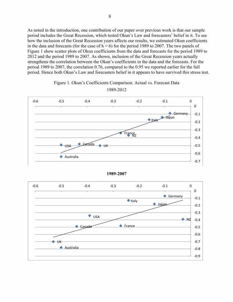
As noted in the introduction, one contribution of our paper over previous work is that our sample period includes the Great Recession, which tested Okun’s Law and forecasters’ belief in it. To see how the inclusion of the Great Recession years affects our results, we estimated Okun coefficients in the data and forecasts (for the case of h = 6) for the period 1989 to 2007. The two panels of Figure 1 show scatter plots of Okun coefficients from the data and forecasts for the period 1989 to 2012 and the period 1989 to 2007. As shown, inclusion of the Great Recession years actually strengthens the correlation between the Okun’s coefficients in the data and the forecasts. For the period 1989 to 2007, the correlation 0.76, compared to the 0.95 we reported earlier for the full period. Hence both Okun’s Law and forecasters belief in it appears to have survived this stress test.

Figure 1. Okun’s Coefficients Comparison: Actual vs. Forecast Data

1989-2012

1989-2007

USA

JapanGermany

France

Italy

UKCanada

Australia

NZ

-0.7

-0.6

-0.5

-0.4

-0.3

-0.2

-0.1

0

-0.6 -0.5 -0.4 -0.3 -0.2 -0.1 0

USA

Japan

Germany

France

Italy

UK

Canada

Australia

NZ

-0.9

-0.8

-0.7

-0.6

-0.5

-0.4

-0.3

-0.2

-0.1

0

-0.6 -0.5 -0.4 -0.3 -0.2 -0.1 0

9

In their comment on our paper, Guisinger and Sinclair (2014) provide another check of robustness by comparing the Okun coefficient from the forecasts with those computed from real-time data. As they report, the correlation between the two sets of coefficients is 0.60, and even higher (0.88) if two outliers are excluded. We conclude this section by discussing briefly how our results relate to some findings in the literature and noting some areas for further work. Most studies have found considerable cross-country variation in Okun’s coefficients in both data and forecasts. While the findings are not uniform across studies, many find low Okun coefficients for Japan and Germany, which is the case with our results as well. Pierdzioch and others (2011) find a small Okun’s coefficient for Japan in the individual forecast data; as they note, this mirrors findings of low Okun’s coefficients in Japanese data in studies by Paldam (1987), Moosa (1997), Lee (2000) and Freeman (2001).7 We leave for future work tests of whether the relationship between forecasts of unemployment and real GDP displays asymmetries or has undergone structural breaks. With respect to asymmetries, Silvapulle, Moosa and Silvapulle (2004) find that in data for the United States the response of unemployment to output is stronger when the output gap is negative than when the gap is positive. In forecasts for G-7 countries, Pierdzioch and others (2011) found some evidence of asymmetry for the United States, but it was sensitive to the choice of horizon; they did not find any evidence of asymmetries in forecasts for the other six G7 countries. With respect to structural breaks, Ball and others (2013) found no evidence of a structural break in the Okun’s Law relationship for the United States. For other countries, Sogner and Stiassny (2002) and Ball and others (2013) find some evidence of changes in the Okun coefficient. For a set of 20 OECD countries, Ball and others (2013) do a check for stability by estimating separate coefficients for the first and second halves of their sample, 1980–1995 and 1996–2011. They find that for seven of the 20 countries, they can reject equality of the coefficients at the five percent level; three of those countries are part of our sample, Canada, Japan and the UK.

IV. EVIDENCE FROM FORECAST REVISIONS

We exploit the availability of repeated revisions of forecasts to shed further light on whether forecasters believe in Okun’s Law. We define an ‘initial’ revision of the forecast as the change in the year-ahead forecasts between April (h = 21) and October (h = 15) and the ‘final’ revision of the forecasts as the change in current-year forecasts between April (h = 9) and October (h = 3). Results from regressions of revisions of unemployment rate forecasts on a constant plus revisions of GDP growth forecasts are shown in Table 4.8 7 Rülke (2012) uses individual-level forecasts from Consensus Economics for six Asian-Pacific countries (three of which—Australia, Japan and New Zealand—are in our sample) and concludes that “professional forecasters believe in … Okun’s law. This result … is robust when using time-varying coefficients, different forecast horizons and when taking business cycle asymmetries into account. The results also suggest that the confidence in [Okun’s Law] is more pronounced during the economic crisis 2007–2009 and when looking at longer forecast horizons. Interestingly, the coefficients based on the actual series are similar to those based on the forecasts.” 8 An equation specification without a constant term does not alter our results. The results are also robust to the choice of forecast horizon, i.e., changing the months over which the final and initial revisions are calculated.

10

Table 2. Unemployment Rate and GDP Growth Forecast Revisions

Panel A: Year-Ahead Revisions Panel B: Current-Year Revisions

Adj. R2 Adj. R2 United States 0.058* -0.386*** 0.882 0.027 -0.158** 0.118 (0.03) (0.04) (0.04) (0.06) Japan -0.011 -0.194*** 0.684 -0.009 -0.073* 0.122 (0.02) (0.03) (0.04) (0.04) Germany 0.038 -0.362*** 0.417 -0.101* -0.319*** 0.322 (0.06) (0.09) (0.06) (0.06) France 0.007 -0.419*** 0.635 -0.014 -0.198 0.054 (0.05) (0.1) (0.08) (0.14) Italy 0.065 -0.231** 0.353 -0.085 -0.226 0.027 (0.05) (0.09) (0.07) (0.17) United Kingdom -0.075 -0.450*** 0.672 -0.194*** -0.192** 0.184 (0.05) (0.08) (0.05) (0.09) Canada 0.026 -0.333*** 0.748 -0.022 -0.214** 0.232 (0.02) (0.05) (0.05) (0.08) Australia 0.052 -0.373*** 0.369 -0.058 -0.217** 0.327 (0.05) (0.12) (0.04) (0.08) New Zealand 0.005 -0.367*** 0.572 -0.129 -0.222*** 0.212 (0.04) (0.09) (0.09) (0.06)

11

Figure 2. Unemployment Rate and GDP Growth Forecast Revisions

The key result is that in all 18 cases shown in the table, revisions in output growth forecasts and revisions in unemployment forecasts are negatively correlated, consistent with Okun’s Law. They are significantly different from zero in all but two cases.

We also find that the absolute value of the Okun coefficient is higher for the initial revisions than for the final revisions in all nine cases, as illustrated in Figure 2, albeit marginally so in the case of Germany and Italy. The adjusted R2 is also considerably higher in each of the nine cases for the year-ahead revisions than for the current-year revisions. A conjecture for this finding is that at the start of the forecast horizon, when information about likely departures from Okun’s Law is scarce, revisions in output and unemployment should be highly correlated if forecasters believe in Okun’s Law. As the forecast horizon draws to a close, forecasters know more about the likely extent of the deviation from Okun’s Law. At that point, the revisions of output and unemployment should be less correlated, as forecasters start to place greater weight on what they are learning about the likely ‘residual’ from Okun’s Law than on their prior belief in it. Our work assumes that it is revisions in GDP forecasts that drive revisions in unemployment forecasts. In future work, we intend to explore the possibility that the relationship between the two sets of revisions could be more complicated. Data on unemployment and real GDP arrive at different frequencies—the former generally monthly, the latter quarterly—and GDP data are subject to greater revision than unemployment data. In this environment, it would not be surprising if forecasters use the arrival of information about unemployment to adjust their real GDP forecasts.9

9 In preliminary work, we estimated a two variable VAR consisting of (1) monthly revisions to forecasts of unemployment changes and (2) the monthly revisions to real GDP growth forecasts. The impulse responses show that not only do unemployment forecasts respond to an innovation in real GDP forecasts but also that real GDP forecasts respond to innovations in unemployment forecasts. Thus there indeed seems to be a bi-directional relationship that needs to be explored further. Barnes, Gumbau-Brisa and Olivei (2013) find that, in the data, real-time errors in Okun’s Law contain information about future revisions to GDP. It would interesting to see if forecasters are aware of this relationship and use it to revise their GDP forecasts.

-0.6

-0.4

-0.2

0

USA Japan Germany France Italy UK Canada Australia New Zealand

initial final

12

V. CONCLUSIONS

Our results show that professional forecasters believe in Okun’s Law to a degree merited by how well it holds in the data. For all nine countries we study, the relationship between forecasts of changes in unemployment and changes in real GDP growth is negative, which is consistent with Okun’s Law. Moreover, the variation across countries in the Okun coefficient lines up well in the forecasts and the data; in particular, the small magnitudes of the Okun coefficients for Japan, Germany, Italy found in the data also hold true for the forecasts. Forecasters’ belief in Okun’s Law held up during the Great Recession, mirroring its survival in the data. We also find that relationship between revision in unemployment and real GDP forecasts is consistent with Okun’s Law: unemployment forecasts are revised down when GDP forecasts are revised up. Moreover, the correlation between output and unemployment forecast revisions is stronger in year-ahead forecasts than in current-year forecasts; this finding leads us to conjecture that forecasters’ reliance on Okun’s Law is stronger in the early stages of the forecast horizon, when information about the likely departures from Okun’s Law is scarce.

13

Appendix This Appendix describes the basic properties of the forecasts of unemployment and real GDP and a robustness check of the results reported in the Section III of main text of the paper. Properties of forecast Figure 3 contrasts the distributions of real GDP growth and unemployment with the distributions of the forecasts at selected horizons (h = 21, 9, 3, 1) with the distribution in the data. Both data and forecasts are pooled across the nine countries in our sample. The key purpose is to show that the forecasts display the reasonable property that they start to mirror the data as the forecast horizon draws to a close. As the value of h gets smaller, the distribution of the forecasts starts to move closer to the distribution of the data, and the distance between the two has largely vanished at h=1, particularly for real GDP forecasts. We next examine properties of the forecast errors. Ideally, forecast errors would not display bias; moreover, the absolute size of the errors should be smaller for smaller values of h. For each country i during year t, we define , where e represents forecast error, F denotes the

forecast, and A denotes its respective realization.

Table 3. Okun's Law: Current Year Forecasts

Current Year Current Year (h=6; Survey Month: July) (h=9; Survey Month: April)

α β Adj. R2 α β Adj. R2

U.S. 1.38*** -0.49*** 0.66 1.28*** -0.47*** 0.73 [0.29] [0.10] [0.21] [0.07]

Japan 0.32*** -0.14*** 0.58 0.30*** -0.14*** 0.61 [0.06] [0.02] [0.05] [0.02]

Germany 0.77* -0.09 -0.03 0.82* -0.06 -0.04 [0.31] [0.10] [0.29] [0.13]

France 0.89*** -0.34*** 0.25 0.74*** -0.24** 0.11 [0.14] [0.07] [0.15] [0.07]

Italy 0.50** -0.17* 0.1 0.48* -0.17* 0.09 [0.17] [0.06] [0.17] [0.07]

UK 1.03*** -0.50*** 0.73 1.28*** -0.55*** 0.73 [0.20] [0.09] [0.19] [0.08]

Canada 1.09*** -0.48*** 0.79 1.23*** -0.53*** 0.88 [0.14] [0.05] [0.11] [0.03]

Australia 2.04*** -0.64*** 0.64 1.93*** -0.61*** 0.71 [0.48] [0.14] [0.34] [0.10]

N. Zealand 0.94*** -0.37*** 0.51 1.12*** -0.40*** 0.43 [0.14] [0.07] [0.19] [0.06]

Note: This table presents OLS estimates of Eq. (3). Standard errors are reported in parenthesis. *, **, *** indicate significance at 10, 5 and 1% levels, respectively.

ititit FAe

14

In Table 4, the results for h = 18, which are reported in the main text, are compared to those for h = 21. As with the current-year forecasts, the choice of the forecast horizon does not make an appreciable difference; the correlation between the estimates for h=18 and h=21 is 0.98. Comparing with Table 3, we see that there are pronounced differences in the cases of Germany, Italy and New Zealand; in each case the Okun coefficient is considerably larger in absolute magnitude in the case of year-ahead forecasts. Nevertheless, correlation between the current-year and year-ahead estimated remains quite high; for example, the correlation between the estimates for h=6 and h=21 is 0.74. This supports our assertion in the main text that the Okun coefficient estimates from forecasts are not very sensitive to the choice of horizon.

Table 4. Okun's Law: Year-Ahead Forecasts

Year Ahead Year Ahead (h=18; Survey Month: July) (h=21; Survey Month: April)

α β Adj. R2 α β Adj. R2 U.S. 0.96*** -0.36*** 0.36 0.99*** -0.38*** 0.39

[0.21] [0.07] [0.22] [0.08] Japan 0.21* -0.10* 0.13 0.18 -0.09 0.11

[0.10] [0.05] [0.12] [0.05] Germany 0.67 -0.40 0.27 0.63 -0.40 0.30

[0.46] [0.21] [0.46] [0.21] France 0.66** -0.38*** 0.52 0.59* -0.35** 0.44

[0.22] [0.10] [0.26] [0.11] Italy 0.48** -0.32*** 0.63 0.32* -0.25** 0.56

[0.16] [0.08] [0.14] [0.07] UK 1.63*** -0.67*** 0.53 1.57*** -0.63*** 0.59

[0.36] [0.14] [0.18] [0.07] Canada 0.90*** -0.37*** 0.57 0.82** -0.35*** 0.52

[0.21] [0.07] [0.22] [0.07] Australia 1.87** -0.59*** 0.56 1.92** -0.61*** 0.54

[0.52] [0.15] [0.53] [0.15] N. Z. 2.17*** -0.78*** 0.78 1.89*** -0.66*** 0.74

[0.33] [0.11] [0.3] [0.11] Note: This table presents OLS estimates of Eq. (3). Standard errors are reported in parenthesis. *, **, *** indicate significance at 10, 5 and 1% levels, respectively.

15

Figure 3. Distributions of Actual and Forecasted Unemployment Rate and GDP Growth: Consensus 1989-2012

Panel A

Panel B

Figure 4 shows three conventional summary measures of errors, the mean error or bias, the mean absolute error (MAE) and the root mean squared error (RMSE). The horizontal axis of the graphs shows the horizon. The bias in unemployment is negative over the entire horizon; that is, actual unemployment is below the forecast on average. The pattern of the bias is difficult to explain. In any event, the main point to note is that the size of the bias is not large. In the case of GDP growth, the bias is also negative, so that forecasters are over-optimistic throughout the forecast horizon. But here the bias is monotonically eliminated over time, so that by h=1 there is essentially no bias. The MAE and RMSE statistics display the reassuring property that the errors decline systematically over time for both unemployment and real GDP growth. For unemployment, MAE starts out at 1 percent at the start of the horizon (compared against an average value of 7 percent for the sample) and decline to 0.35 percent by the end. For real GDP growth, the MAE for h=24 is rather large compared to the sample average (1.5 percent compared to a sample average of 2.1 percent), but declines to 0.25 percent for h=1.

010

2030

21 m

ont

h ho

rizon

2 4 6 8 10 12

Advanced Economies

010

2030

9 m

onth

hor

izo

n

2 4 6 8 10 12

010

2030

3 m

onth

hor

izo

n

2 4 6 8 10 12

010

2030

1 m

onth

hor

izo

n

2 4 6 8 10 12

Distributions of Actual (Grey) and Forecasted (Black)Unemployment Rate, 1989-2012

020

4060

8010

021

mo

nth

horiz

on

-5 0 5

Advanced Economies

020

4060

8010

09

mon

th h

oriz

on

-10 -5 0 5

020

4060

8010

03

mon

th h

oriz

on

-5 0 5

020

4060

8010

01

mon

th h

oriz

on

-5 0 5

Distributions of Actual (Grey) and Forecasted (Black)GDP growth, 1989-2012

16

Figure 4. Unemployment Rate and GDP Growth Forecast Errors: Consensus 1989-2012

Panel A Panel B

Robustness checks Section III of the main text of the paper provides estimates of the Okun coefficients for h = 6 (which corresponds to July of the current year). In Table 3, these estimates are compared with those for h = 9 (April of the current year). This does not make much of a difference to the Okun coefficient estimates; the correlation between the two is 0.96.

-.3

-.25

-.2

-.15

13691215182124

1

h1

Mean Errors

.2.4

.6.8

1

13691215182124

1

h1

Mean Absolute Errors

.6.8

11.

2

13691215182124

1

Forecast Horizon

Root Mean Squared Errors

Unemployment Rate

-.8

-.6

-.4

-.2

0

13691215182124

1

h1

Mean Errors

.51

1.5

13691215182124

1

h1

Mean Absolute Errors

.51

1.5

2

13691215182124

1

Forecast Horizon

Root Mean Squared Errors

GDP growth

17

References

Ball, L., Daniel Leigh, and Prakash Loungani, 2013, “Okun’s Law: Fit at Fifty,” NBER Working Paper No. 18668, (Cambridge, Massachusetts: National Bureau of Economic Research).

Barnes, Michelle, Fabià Gumbau-Brisa, and Giovanni Olivei, 2013, “Do Real-Time Okun’s Law Errors Predict GDP Data Revisions?” Working Paper 13–3, Federal Reserve Bank of Boston.

Blanchard, Olivier and Stanley Fischer, 1989, Lectures on Macroeconomics (Cambridge: MIT Press). Blinder, Alan, 1997, “Is There a Core of Practical Macroeconomics that We Should all Believe?”

American Economic Review, Vol. 87 (May), pp. 240–43. Fendel, Ralf, Elisa Lis, and Jan-Christoph Rülke, 2011, “Do Professional Forecasters Believe in

the Phillips Curve? Evidence from the G7 Countries,” Journal of Forecasting, Vol. 30 (March), pp. 268–87.

Freeman, Donald, 2001, “Panel Tests of Okun’s Law for Ten Industrial Countries,” Economic

Inquiry, Vol. 39 (October), pp. 511–23. Guisinger, A. and T. Sinclair, 2014, “Okun’s Law in Real-time,” forthcoming. Lee, Jim, 2000, “The Robustness of Okun’s Law: Evidence from OECD Countries,” Journal of

Macroeconomics, Vol. 22 (April), pp. 331–56. Mankiw, N. G., 2012, Macroeconomics, Eighth Edition, Worth Publishers. Mitchell, Karlyn and Douglas Pearce, 2010, “Do Wall Street Economists Believe in Okun’s Law

and the Taylor Rule?” Journal of Economics and Finance, Vol. 34 (April), pp. 196–17. Moosa, Imad, 1997, “A Cross-country Comparison of Okun’s Coefficient,” Journal of

Comparative Economics, Vol. 24 (June), pp. 335–56. Okun, Arthur, 1962, "Potential GNP: Its Measurement and Significance," Proceedings of the

Business and Economics Statistics Section, American Statistical Association, pp. 89–104. Paldam, Martin, 1987, “How Much Does One Percent Growth Change the Unemployment Rate?

A Study of 17 OECD Countries, 1948-1985,” European Economic Review, Vol. 31, No. 1-2, pp. 306–13.

Pierdzioch, Christian, Jan-Christoph Rülke, and Georg Stadtmann, 2011, “Do Professional

Economists’ Forecasts Reflect Okun’s Law? Some Evidence for the G7 Countries,” Applied Economics, Vol. 43, No. 11, pp. 1365–73.

Romer, David, 2012, Advanced Macroeconomics, Fourth Edition, The Mcgraw-Hill.

18

Rülke, Jan-Christoph, 2012, “Do Professional Forecasters Apply the Phillips Curve and Okun's Law? Evidence from Six Asian-Pacific Countries,” Japan and the World Economy, Vol. 24 (December), pp. 317–324.

Silvapulle, Paramsothy, Moosa, Imad and Mervyn Silvapulle, M, 2004, “Asymmetry in Okun's

Law,” Canadian Journal of Economics, Vol. 37, No. 2, pp. 353–374. Sinclair, Tara, Stekler, H.O., and Warren Carnow, 2014, “A New Approach for Evaluating

Economic Forecasts,” forthcoming. Sögner, Leopold and Alfred Stiassny, 2002, “An Analysis on the Structural Stability of Okun's

Law—A Cross-country Study,” Applied Economics, Vol. 34, No. 14, pp. 1775–87. Tillmann, Peter, 2010, “Do FOMC Members Believe in the Okun’s Law?” Journal Economic

Bulletin, Vol. 30, No. 3, pp. 2398–04.