Institut de Recerca en Economia Aplicada Regional i Pública Document de Treball 2015/01 1/37 Research Institute of Applied Economics Working Paper 2015/01 1/37

Grup de Recerca Anàlisi Quantitativa Regional Document de Treball 2015/01 1/37 Regional Quantitative Analysis Research Group Working Paper 2015/01 1/37

“An analysis of the Okun’s law for the Spanish provinces”

Celia Melguizo Cháfer

WEBSITE: www.ub-irea.com • CONTACT: irea@ub.edu

WEBSITE: www.ub.edu/aqr/ • CONTACT: aqr@ub.edu

Universitat de Barcelona Av. Diagonal, 690 • 08034 Barcelona

The Research Institute of Applied Economics (IREA) in Barcelona was founded in 2005, as a research institute in applied economics. Three consolidated research groups make up the institute: AQR, RISK and GiM, and a large number of members are involved in the Institute. IREA focuses on four priority lines of investigation: (i) the quantitative study of regional and urban economic activity and analysis of regional and local economic policies, (ii) study of public economic activity in markets, particularly in the fields of empirical evaluation of privatization, the regulation and competition in the markets of public services using state of industrial economy, (iii) risk analysis in finance and insurance, and (iv) the development of micro and macro econometrics applied for the analysis of economic activity, particularly for quantitative evaluation of public policies.

IREA Working Papers often represent preliminary work and are circulated to encourage discussion. Citation of such a paper should account for its provisional character. For that reason, IREA Working Papers may not be reproduced or distributed without the written consent of the author. A revised version may be available directly from the author.

Any opinions expressed here are those of the author(s) and not those of IREA. Research published in this series may include views on policy, but the institute itself takes no institutional policy positions.

Abstract

The inverse relationship between unemployment and Gross Domestic Product (GDP) growth, commonly known as Okun’s law, has been traditionally analysed in the economic literature. Its application for Spain has been carried out at the national level or for the autonomous communities but it has not been analysed for provinces, the territorial level closer to local labour markets. This study analyses this relationship during the period spanning from 1985 to 2011. After testing the time series properties of provincial GDP and unemployment, we specify statiic and dynamic versions of the Okun’s law using VAR and PVAR techniques. Both static and dynamic analyses lead us to determine that provinces show large differences in their unemployment sensitivity to GDP shocks. In particular, provinces where economic activity is concentrated and Southern provinces are those suffering from higher cyclical variations in unemployment rates.

JEL classification: C32, C33, J23, R11 Keywords: Unemployment, Output fluctuations, Spanish provinces

Celia Melguizo Cháfer. AQR Research Group-IREA. Department of Econometrics. University of Barcelona, Av. Diagonal 690, 08034 Barcelona, Spain. E-mail: cmelguizo@ub.edu �

Acknowledgements

1. Introduction

The strong impact of business cycles on unemployment is a Spanish particular

feature. The high increase in unemployment during the current economic downturn is a

clear example of this great variability of the unemployment rate. Since 2008 and in just

six years the unemployment rate has more than tripled, accounting in 2013 for 26% of

the working population. However, this phenomenon is not confined to recession

periods. Before this economic crisis, Spanish economy had experienced a continuous

growth reducing unemployment rates from 20% of the labour force population to levels

slightly above the European average.

Nevertheless, unemployment sensitivity to Gross Domestic Product (GDP) shifts

is not the same for all regions. Villaverde and Maza (2009) found that whereas in some

regions a great unemployment response to changes in the economic cycle is observed,

in others unemployment rate varies to a lesser extent. They attributed these differences

to the unequal growth of productivity between regions. But, analysing the differences

regarding the impact of GDP on unemployment for autonomous communities could be

somehow misleading. It is important to consider regional units that are closer to local

labour markets, as this is the territorial dimension that really matters to firms and

workers. In fact, autonomous communities show great internal differences in the level

of economic activity, diverse urbanization degree and lack of uniformity in the

productivity level and productivity growth. In this regard, the provincial approach

implies a thorough and rigorous analysis that provides more light to the patterns and

differences in the unemployment sensitivity to economic variations. Still in the regional

analysis, provincial approach situates us closer to the local level.

Therefore, the aim of this paper consists in analysing the differences between

provinces in the unemployment response to GDP variations. In order to do so, we

consider static and dynamic specifications to determine the relationship between the

aforementioned variables for all Spanish provinces. Firstly, the static analysis is carried

out by using the difference version of the Okun’s law, whereas VAR techniques are

used to perform the dynamic analysis. The analysis is complemented using panel and

PVAR models in order to compare provincial results with the aggregate dynamics of

unemployment and GDP.

Our results show that there are great differences between provinces regarding the

unemployment sensitivity to variations in economic conditions. Both static and dynamic

analysis suggest that provinces where economic activity is concentrated and southern

provinces are those ones that suffer to a higher extent the impact of GDP shocks on

unemployment.

This finding justifies resorting to a provincial approach as we also find that

autonomous communities are not homogenous. So, one of the contributions of this

paper concerns the need to consider a provincial approach when we analyse the Spanish

labour market from a regional perspective. It has not been carried out previously in

studies examining Okun's law for Spain. This new scope of analysis offers interesting

results that should be taken into account when economic policies are defined. The

second contribution consists in performing a dynamic analysis of the Okun’s law

through VAR and PVAR techniques, which have not been applied at the Spanish

provincial level yet.

The rest of the paper is organized as follows. In section 2, we briefly gather the

contributions to Okun's law, including specific analysis for Spain.. In section 3, we

describe the methodology that we undertake and section 4 presents the main results that

we obtain. Finally, section 5 concludes.

2. Literature review

2.1. General overview

The relationship between economic activity and unemployment has been

traditionally analysed by using the different specifications of Okun’s law.1 Okun

(1962) formulated the well-known rule of a thumb that assigns approximately a 3

percentage – point of GDP decrease to a 1 percentage – point of unemployment rate

increase. Since then, it has been the focus of discussion and analysis. Many authors

have submitted it to transformations in order to modify certain theoretical foundations

and to achieve a more accurate statistical fit. Furthermore, it has been applied to

different economic contexts. It is worth noting the work of Gordon (1984), Evans

1 Okun's law is an empirically observed relationship relating unemployment to GDP. The initial statement of this law supposes that a 3% increase in output corresponds to a 1% decline in the rate of unemployment.

(1989), Prachowny (1993), Weber (1995), Attfield and Silverstone (1997), Knotek

(2007), Owyang and Sekhposyan (2012) and Perman et. al. (2014), among others.

The different authors have defined both static and dynamic specifications of the

aforementioned empirical relationship. For instance, Evans (1989) considered three

lagged periods in order to observe how past variations in Gross National Product (GNP)

and unemployment influenced quarterly values of these variables. He applied a bivariate

approach and obtained instantaneous causality and a significant long run relationship

between GNP and unemployment rate.

Economists have also analysed the relationship between GDP and

unemployment rate in two additional directions. First, whereas Okun seminal study

considered unemployment as the exogenous variable, other relevant analysis placed it

endogenously. Thus, Okun’s coefficient comparisons between both kinds of studies turn

out worthless. Second, another transformation undergone by the empirical relationship

has consisted in introducing new variables in the original formula. For instance, Gordon

(1984) introduced as explanatory variables the changes in capital and technology

regarding their potential level, besides unemployment variations. Prachowny (1993)

considered labour supply, workers weekly hours and capacity utilization deviations

from the equilibrium additionally.

All these transformations have contributed to the fact that there is no consensus

about the value of the Okun’s coefficient. Some authors have confirmed the value

initially presented by Okun. Others obtained that the magnitude of the impact of

business cycle on unemployment is closer to two instead of three. Finally, there are

analyses that show that the Okun’s coefficient varies over the period selected and

among the countries considered.

Weber (1995) analysed the U.S. economy during the period 1948-1988 and

obtained that the long-term coefficient was close to three. However, he acknowledged

there was a breakdown in the third quarter of 1973. In the same line, more recent studies

such as Knotek (2007) and Owyang and Sekhposyan (2012) considered this empirical

relationship is a good approximation in the long term, but they showed the coefficient

has not been kept stable over the time.

In this regard, Perman et. al. (2014) conducted a meta-analysis to obtain the

“true value” of the Okun’s law coefficient. In order to do so, they used a sample of 269

estimates. Among these, they discarded those ones that did not fulfil the pre-established

requirements and distinguished between the analyses that considered changes in GDP as

the independent variable and the studies that considered unemployment variations

exogenously. They quantified the impact of unemployment rate on GDP in -1.02 points.

This value is far away from the three points - coefficient and make obvious that the

period and countries selected matters. In the same vein, Lee (2000) acknowledged that

Okun's law could be considered valid qualitatively, but not quantitatively. He selected

16 OECD countries to observe if the so - called rule of thumb holds. Lee obtained that,

although all countries present a negative relationship between GDP and unemployment,

the coefficient that relates these variables varies significantly across countries. Moosa

(1997), who considered the G7 countries, had previously obtained the same result.

Therefore, the fact that a significant negative relationship between

unemployment and GDP could be accepted for almost all countries and for any period is

an interesting empirical result. However, the coefficient divergence across countries and

over time is one of the most important criticisms2.

2.2. From the national to the regional perspective

The main criticism of Okun's law, based on the divergence in its coefficient, has

become a tool to compare the labour market performance in the different countries and

regions. The regional analysis further allows isolating the impact of labour market

institutions. For this reason, many authors have figured out the patterns of

unemployment and business cycle by region as well as their relationship to determine

the appropriate economic policies to apply.

One of the first authors to apply the Okun’s law at regional level was Freeman

(2000). He applied it to eight U.S. areas and obtained, unlike the studies that we

mention later, a similar and stable coefficient for all regions. This result shows a high

flexibility in the U.S. labour market that favours regional convergence in the

unemployment rates. However, Adanu (2005) did not get this level of convergence

2 But this is not the only one. From a labour economics perspective, many authors recognize that unemployment rate does not provide comprehensive information from the labour market situation. In this regard, Benati (2001) and Emerson (2011) established that it leaves out the “discouraged worker” effect, i.e., the unemployed who drop out the labour market as they give up hope about being employed. As a result, this group become part of the inactivity. On the other hand, the “added worker” effect (the entry of inactive in the labour market due to an adverse economic situation), which has been considered by Congregado et. al. (2011), also modifies the unemployment rate.

among Canadian provinces. Moreover, he obtained that the law did not hold for three of

the ten provinces analysed. Adanu analysed how unemployment affects GDP during the

1981-2001 period for the Canadian provinces and observed GDP highly varies in the

most industrialized provinces when changes in labour occur. This is mainly due to

productive jobs are in a greater extent in industrialized provinces.

In European countries, Okun’s law holds at national level but when regions are

analysed, some authors obtain that variations in business cycle do not always explain

the changes in the unemployment rate. Binet and Facchini (2013) applied the

relationship to the twenty-two French regions and obtained it is significant for only

fourteen of them. They show it is due to high unemployment rates coexist in some

regions with above average per capita GDP levels. According to the authors, such

situation out of equilibrium is partly a result of a rapid growth of working-age

population that has not been absorbed by an employment increase. Also, the great

percentage of public sector employment in the regions where the Okun’s law does not

hold hampers the adjustment to equilibrium.

Lack of significance of Okun’s law is even more extended in the Greek regions.

Christopoulos (2004) applied a similar analysis to Greek regions and obtained that only

six of thirteen have a significant relationship between unemployment and the business

cycle. Moreover, the coefficients point out much higher unemployment sensitivity to

GDP variations than in North America. Contrarily to Canadian provinces, most

industrialized regions in Greece do not show a significant relationship between

unemployment and GDP, probably due to hysteresis in unemployment.

2.3. The specific case of Spain

The Spanish economy has been characterized by a strong impact of business

cycles on unemployment since 1975. In fact, unemployment rate has experienced an

upward trend that has only undergone two breakdowns during 1986-1991 and 1995-

2007 expansion periods. This unemployment uptrend cannot be justified by the

moderate increase in the labour force participation at the national level.

The economic depression, which affected Spanish economy since 1975, was

mainly attributable to the great instability that took place during the transition to

democracy, the shocks produced in the industry as a result of the delayed effect of the

oil price increase and the social measures that partly geared to augment wages. As a

consequence, in 1985 unemployment rate reached 21.4% and only 47% of the

population was occupied. But, in 1986, the entry into the European Union caused a

widespread optimism that affected the economy and led to a fall in the unemployment

rate. This lasted until 1991, when a generalised recession affected the Spanish economy.

The cycle change came again in 1995 when labour law reforms favoured wage

moderation and boosted temporary jobs. A fuelled housing sector development,

favoured by low interest rates after the euro adoption, promoted the economic growth

and the convergence to the European levels of unemployment occurred. In 2007,

whereas the average unemployment rate was around 7% in Europe, in Spain it was at

8%. This degree of unemployment rate variation illustrates the strong impact that GDP

has on unemployment in Spain, resulting in a greater Okun’s coefficient for this country

than for most OECD ones. Since 2007, the bursting of the housing bubble triggered an

unprecedented recession and in three years, an increase in the unemployment rate of

nearly 12 percentage points occurred. This unemployment increase was accompanied by

only a 7.8 percentage - point GDP drop, which reinforces the assumption of the high

unemployment variability in Spain.

On the other hand, labour force participation has seemed to be alien to these

cycles. It maintained a growing trend that just stalled during 1991-1996 period. This is

illustrated by Jimeno and Bentolila (1998), who acknowledge that changes in the

Spanish economy have been reflected in the unemployment rate. They also consider this

Spanish feature is not commonly observed in the U.S. and most European countries.

There, shocks have a greater impact on migration flows and participation respectively.

But, this is not the whole story. National data do not pick up the great diversity

that Spanish regions show. There are large disparities between regions in terms of the

unemployment rate and unemployment elasticity to business cycles. This is shown by

Pérez, et. al. (2002) and Amarelo (2013). They analysed the cases of Andalusia and

Catalonia respectively and compared them with the Spanish results. Pérez, et. al. (2002)

obtained for Andalusia a lower unemployment variability to business cycles during the

1984-2000 period than it was obtained for Spain, although when the employment rate

was taken into account instead unemployment rate, they cannot find significant

differences from the Spanish value. Meanwhile, Amarelo (2013) observed that

unemployment variability in Catalonia was higher than that obtained for Spain.

Villaverde and Maza (2007, 2009), who observed the Okun’s law for all Spanish

regions, attributed the differences between regions to the productivity growth. They

obtained neither development degree nor spatial patterns can explain these differences.

 

3. Data sources and methodology

3.1. Data sources and variable definition

The analysis of the effect of the output variation on the unemployment rate

requires three macroeconomic data sets: real GDP, unemployment and labour force

participation data. The analysis is carried out annually at provincial level and the period

we focus is spanning between 1985 and 2011. The selected period allows us to consider

the entry of Spain into the European Union and the industrial reconversion, which took

place right after this event, the creation of the welfare state, the economic expansion,

partly dependent on an oversized housing sector, and the recent crisis that began in 2008

and still persists. Meanwhile, province as the unit of analysis implies a thorough study

that specifically takes into account each area weaknesses and allows defining individual

policies that will have greater impact. The number of selected Spanish provinces for the

analysis is 50, excluding Ceuta and Melilla. The information has been taken out from

the Spanish National Institute of Statistics (INE). We resort to the Contabilidad

Regional de España CRE (Spanish Regional Accounts) to obtain nominal GDP by

province and the Índice de Precios al Consumo IPC (Consumer Price Index CPI) data

set to deflate nominal output and obtain a proxied measure of real GDP. Using CPI as

GDP deflator is a consequence of the GDP deflator lack of data at the provincial level

for part of the considered period. INE only supplies information about rates of variation

of real GDP by region, hence provincial CPI becomes the most suitable indicator to

remove the effect of prices in the output. Furthermore, unemployment and labour force

participation information, which is required to draw up the unemployment rate, is

provided by the Encuesta de Población Activa EPA (Labour Force Survey).

TABLE 1

INE provides us non homogeneous panel data sets. Nominal GDP is in different

year basis and we have to homogenize it taking 2011 as the year basis. Moreover, CPI is

only available for provinces after 1993 and we use the index for the provincial capitals

in the previous years. Meanwhile, occupation and participation data are furnished

according to different criteria based on the time when information was collected. In this

case, we follow De la Fuente (2012), who makes the required adjustments in order to

link the 1976-1995 and 1996-2004 occupation and participation series to the 2005-2013

series. The differences are mainly due to sample replacement and methodological

changes such as questionnaires modifications and adjustments in the definition of

occupation and unemployment. These annual and state adjustments are distributed

among the provinces considering their weighting in the state occupation and labour

force participation data.

3.2. Methodology

The analysis of the relationship between output and unemployment requires

checking that series are stationary as a first step. Firstly, we do it for every province and

afterwards, we aggregate all provincial series in a panel that is tested by the panel unit

root tests we mention later. Then, we estimate the relationship between GDP and

unemployment. We use the difference version of the Okun’s law and estimate it by

using Ordinary Least Squares (OLS) and Fixed Effect (FE) for provinces and the panel

respectively. Finally, we perform a dynamic analysis by using VAR and PVAR

techniques.

3.2.1. Unit Root Testing

Unit root testing is a necessary procedure before estimating. It allows us to know

whether the processes generated are stationary and, therefore, the obtained results are

not spurious and have economic sense. Augmented Dickey-Fuller (ADF) and the

Philips-Perron (PP) are some of the most applied tests. In both, the null hypothesis

assumes that series are generated by integrated processes whereas the alternative

establishes the series are stationary. The difference between them is in the way the serial

correlation problem is dealt. Whereas ADF introduces additional lags as regressors of

the variable that is susceptible to present a certain autocorrelation degree, PP makes a

non-parametric correction of the t-test statistic, i.e., PP test uses Newey–West (1987)

standard errors to account for serial correlation. ADF test obtain better results for finite

samples, but PP is robust to heteroskedasticity and unspecified autocorrelation.

However, these traditional unit root tests do not consider the existence of

structural breaks in the series. So, the presence of structural breaks would provoke that

ADF and PP tests tend to have low power. Glynn et. al. (2007) establish that structural

breaks generate a bias in ADF and PP tests that reduces their ability to reject a false unit

root hypothesis. Perron (1989) was the first author to mention this and he developed a

procedure based on the ADF test that accounted for only one exogenous break. His

analysis broke with the idea proposed by Nelson and Plosser (1982), who stated random

shocks were not transitory and did have permanent effect in the economies. However,

the Perron procedure is severely criticised by many economists. Some of them are

Christiano (1992), who established that a pre-test analysis of the data could lead to bias

in the unit root test or Zivot and Andrews (1992), who proposed an endogenous

determination of the break to reduce this bias. The Zivot-Andrews test allows for a

structural break, which is registered the time period in which ADF t-statistic is the

minimum. Later versions, such as Perron and Vogelsang (1992) distinguish between

additive and innovative outliers. Clemente, Montañés and Reyes (1998) contemplate

this break distinction, but they go further and consider the existence of two breaks. In

our study, we conduct the ADF and PP traditional tests but we also apply Zivot-

Andrews and Clemente-Montañés-Reyes tests, which assume structural breaks in the

series. Applying both kinds of tests guarantees robustness in determining if the series

are stationary. The lag length selection criterion has been different for each test. For the

ADF test, we have observed for every province the lags that are significant at 90% level

and we have chosen the maximum number of significant lags. Meanwhile, we have

recurred to the default number of Newey-West lags to calculate the standard error for

the PP test.3

After conducting individual unit root tests, panel-data unit root tests are applied

in order to complete our analysis and get an overall view of the GDP and the

unemployment rate of the Spanish provinces. They give additional information and

increase the value of unit root tests based on single series. There is some literature about

them and many attempts to remove cross-sectional dependence such as Pesaran (2007),

Moon and Perron (2004), Maddala and Wu (1999), Levin-Lin (2002) and Im-Pesaran-

Shin (2003). In our work we apply the Fisher-type, Levin Lin Chu, Im Pesaran Shin and

Hadri LM tests. In the first three tests, the null hypothesis considers the presence of unit

roots in, at least, one of the series that form the panel and stationarity is assumed under

the alternative hypothesis. Otherwise, Hadri LM test considers in its null hypothesis that

the series are generated by stationary processes. Hadri test is an extension of

Kwiatkowski et. al.(1992) tests for panel data and it provides us added value due to, as

Hadri (1999) acknowledges, by testing both the unit root and the stationary hypothesis

we are able to make a distinction between the stationary series, the series that have

unit roots and those ones for which we are not sure if they are stationary or integrated.

In all the tests the lag length4 is chosen according to Österholm (2004), who

selects the maximum number of lags from the individual tests. The maximum

significant number of lags obtained in the individual ADF test is that we use to

determine the lag length for the panel unit root tests.

3.2.2. Okun’s law specifications

3 This number of lags is given by the following formula: int{4(T/100)2/9}.

4 Other criteria are also used in order to obtain robust results. We also consider the AIC criterion in the Levin Lin Chu and Im Pesaran Shin tests to select the lag length.

Once we know that the series that we are working with are stationary, we can

figure out the relationship between GDP and unemployment variables and then analyse

their dynamics.

In order to observe the relationship that the aforementioned variables maintain,

we resort to the difference version of the Okun's law.

(ut – ut-1) = α + β1(yt - yt-1) (1)

where ut – ut-1 represents the difference between unemployment rates in periods t and t-

1, yt – yt-1 is the variation of the GDP natural logarithm that takes place between t and t-

1 periods. This specification is considered in our analysis due to the unobservability of

the potential magnitudes of the variables taken into account, which are considered in the

gap version. In addition, the large variability in the unemployment rate observed for

Spain and many of its provinces over the selected period makes our specification

becomes more accurate than the gap approach. The estimation of the coefficient of

provincial series is performed by using the Ordinary Least Squares method (OLS)

method, while the panel that integrates all provinces requires estimating by fixed effects

(FE).

The dynamic behaviour of economic growth and unemployment rate variation is

analysed through the VAR and PVAR techniques. It allows us to consider the effect that

past values of both variables have on each of them. We can write VAR representation as

follows:

Δut = α(L)Δut-1 + β(L)Δyt-1 + vtu

Δyt = γ(L)Δyt-1 + η(L)Δut-1 + vty (2)

where Δut and Δyt represents respectively unemployment rate and GDP natural

logarithm variations between periods t and t-1; α(L), β(L), γ(L) and η(L) are respectively

the vectors of the coefficients relating past values of the variables associated to current

values; vtu and vt

y are vectors of the idiosyncratic errors.

The VAR analysis allows answering the question of what is the effect of an

output or unemployment innovation regarding past values of these variables. VAR

models treat GDP and unemployment variables as endogenous and interdependent and

analyse the transmission of idiosyncratic shocks across time. Meanwhile, the panel that

includes all provincial series requires the PVAR technique5. The lag order selected in

these dynamic analyses is one because we work with annual data and we expect that the

variables considered keep some correlation with the same variable lagged one period.

The AIC and BIC criteria also obtain that considering one lag in the VAR analysis is

optimal for most series.

After performing the estimation, Impulse Response Functions (IRFs) associated

show the response of both variables to shocks in any of them. We obtain them for all the

provinces by orthogonalising the variables.

4. Empirical results

The Spanish unemployment rate has experienced a great variability relative to

variations in GDP. The crises have resulted in large increases in unemployment, while

economic expansions have also meant higher falls in the unemployment rate than initial

statement of the Okun’s law forecasted. Provinces have suffered differently the

unemployment sensitivity to GDP variations. In this section, we explore the Okun’s

relationship for all provinces and the panel to detect the unemployment behaviour

regarding output fluctuations and their dynamics. In order to do so, we firstly conduct

the tests that prove the stationarity of the series employed and then we perform the static

and dynamic analyses to estimate the aforementioned empirical relationship.

5 In order to apply PVAR technique, we resort to Ryan Decker program, which is an update version of the Inessa Love original package, which is used in Love and Zicchino (2006), among others.

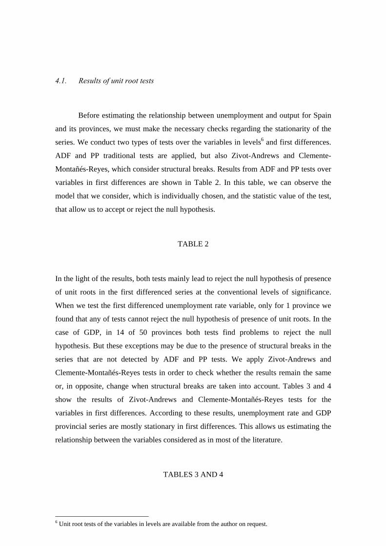
4.1. Results of unit root tests

Before estimating the relationship between unemployment and output for Spain

and its provinces, we must make the necessary checks regarding the stationarity of the

series. We conduct two types of tests over the variables in levels6 and first differences.

ADF and PP traditional tests are applied, but also Zivot-Andrews and Clemente-

Montañés-Reyes, which consider structural breaks. Results from ADF and PP tests over

variables in first differences are shown in Table 2. In this table, we can observe the

model that we consider, which is individually chosen, and the statistic value of the test,

that allow us to accept or reject the null hypothesis.

TABLE 2

In the light of the results, both tests mainly lead to reject the null hypothesis of presence

of unit roots in the first differenced series at the conventional levels of significance.

When we test the first differenced unemployment rate variable, only for 1 province we

found that any of tests cannot reject the null hypothesis of presence of unit roots. In the

case of GDP, in 14 of 50 provinces both tests find problems to reject the null

hypothesis. But these exceptions may be due to the presence of structural breaks in the

series that are not detected by ADF and PP tests. We apply Zivot-Andrews and

Clemente-Montañés-Reyes tests in order to check whether the results remain the same

or, in opposite, change when structural breaks are taken into account. Tables 3 and 4

show the results of Zivot-Andrews and Clemente-Montañés-Reyes tests for the

variables in first differences. According to these results, unemployment rate and GDP

provincial series are mostly stationary in first differences. This allows us estimating the

relationship between the variables considered as in most of the literature.

TABLES 3 AND 4

6 Unit root tests of the variables in levels are available from the author on request.

As previously mentioned, we have also carried out panel unit root tests. Results

are shown in Table 5 and confirm the results obtained for provincial series: unit root

processes are found in the levels of the variables while we cannot reject stationarity in

first differences. In particular, the Levin Lin Chu, Im Pesaran Shin and Fisher Type

(conducted as an ADF test) tests reject the null hypothesis of unit root processes in the

first differenced variables at 99% confidence level. Meanwhile, Hadri LM test cannot

reject stationarity at any of the conventional confidence levels.

TABLE 5

4.2. Static analysis

In this section we estimate the relationship between GDP and unemployment.

We construct a first difference specification for the provinces and the panel that

integrates all of them. The estimation of the provincial series is performed by the

method of ordinary least squares (OLS) while the panel requires estimating by fixed

effects (FE).

The results of the estimation of the Okun’s relationship for the Spanish provinces and

the provincial panel are shown in table 6. Coefficients point out the influence that a

percentage point of GDP variation has on the rate of unemployment. We have ordered

the provinces attending the value of this coefficient and we can observe the great

differences between them. Whereas for some provinces such as Barcelona or Cádiz a

percentage point of GDP variation is accompanied by a change in the opposite direction

of the unemployment rate whose value is higher than 0.6, for Palencia, Cáceres or

Guadalajara GDP shifts barely affect unemployment. The absolute value of the

relationship coefficient does not reach 0.2 percentage points. This is a clear example of

the divergence in the Spanish labour market. There are some provinces where

unemployment highly responds to shifts in the economic activity, whereas some others

show low variability or even not present any relationship. Map 1 shows that provinces

that present greater unemployment sensitivity to GDP variation are the southern ones as

well as the provinces where economic activity is concentrated. This distinction is

because sensitivity to business cycles in these two groups of provinces is presumably

due to different causes. Madrid, Barcelona, Valencia or Zaragoza are provinces where

the respective autonomic capital is. Also, in these provinces large population is

concentrated, they are mostly urban areas and show a high level of economic activity.

Whereas the south is a traditional depressed area where unemployment is accompanied

by lack of economic activity. In the peninsular centre, with the exception of Madrid, and

in the north of Spain is observed that employment remains much more stable. It is

affected in a lesser extent by cyclical changes in the economy. Meanwhile, panel

estimation states that a percentage point of variation in GDP result in an unemployment

rate change in the opposite direction that is quantified in 0.353 percentage points. This

value is not comparable with that obtained by other authors for Spain due to panel

estimation gives equal weight to all regions, so in this case it yields a downward biased

value of the Okun’s coefficient. This is because very populous provinces that present

higher unemployment and economic activity in absolute terms are among those having

greater unemployment sensitivity to GDP variations.

TABLE 6

MAP 1

4.3. Dynamic analysis

The dynamic analysis allows us to observe the effect of economic growth shocks

on unemployment, but also the impact of innovations in unemployment rate variation on

GDP growth. However, as we did earlier in the static analysis, we mainly focus in the

first issue.7 Through the VAR technique, we observe for all provincial series the effect

on unemployment rate of the GDP growth disturbances regarding past values of

unemployment rate variation and economic growth. The impulse response functions

associated (IRFs) shows in an easily interpretable way this effect. So, we have estimated

a bivariate VAR for all provinces and we have obtained their orthogonal impulse-

response functions. The orthogonal IRF representations for all Spanish provinces are

reported in Figure 1. The effect of GDP growth shocks is observed for 6 periods. The

confidence bands are defined by the grey shaded area that is around the line that points

7 Full results from the VAR and PVAR analysis are available from the author on request.

out the effect of GDP growth shocks on unemployment. We can observe that for all

provinces the effect of shocks on unemployment is negative but the magnitude of these

shocks and the persistence varies across provinces. In provinces such as Cádiz, Jaén or

Valencia the initial effect of the shock is very sharp, whereas in Barcelona, Madrid or

Sevilla this initial effect is not so steep but the shock is more persistent. There are also

provinces for which we cannot observe any impact on unemployment. This is the case

of Albacete or Zamora, among others. As in the static analysis, we observe that

provinces greatly differ in their unemployment response to economic shifts. In this case,

the characteristics of the technique employed allow us to observe not only the effect of

the shock in the period when it occurs, but also the impact that this shock has over time.

Table 7 shows for the Spanish provinces the impact of these shocks in the period when

they occur as well as the cumulative effect after 2, 4 and 6 periods. We have ordered the

provinces attending the magnitude of impact of the shock. In the top of the table are the

provinces for which the cumulative effect of the shock is higher at period 6. Again, we

can find in the first positions of the table the provinces where economic activity is

concentrated and some southern provinces. The bottom is composed by the provinces

for which the static analysis acknowledged the impact of GDP on unemployment was

relatively low or not significant. Map 2 gathers in a clearer way the cumulative effect of

GDP growth shocks on unemployment. As we have previously mentioned, we get

results comparable to those obtained in the static analysis. In this case, Málaga are not

between the provinces with higher sensitivity to GDP shifts. Contrarily, Almería,

Badajoz and Huelva does become part of this group. Peninsular centre remains the

geographical area where lower effect of GDP shocks on unemployment is observed.

FIGURE 1

TABLE 7

MAP 2

After observing for all provinces the effect of economic growth shocks, we

apply the PVAR technique in order to observe the effect of shocks for the panel that

integrates all Spanish provinces. In this case, we show the effect that unemployment and

GDP shocks have on themselves and on the other variable. As can be expected the

effect that a shock in the output growth generates on itself is positive. The same occurs

for the first differences of the unemployment rate variable. The effects that shocks have

on the other variable are negative. It should be mentioned that the effect that an

unemployment rate growth shock has on economic growth takes place after one period

due to we have orthogonalized the variables. GDP growth affects unemployment rate

variation contemporaneously, but unemployment rate variation affects economic growth

with a lag. Results from PVAR analysis can be observed in Figures 2 and 3. They show

the IRFs representations when a shock in economic growth and a shock in

unemployment rate variation are respectively produced. The standard errors are

calculated using Monte Carlo simulations with 500 replications. From these figures, we

can draw that the GDP growth shocks have higher effect on both variables than the

unemployment shocks. This is also observed in Table 8, which shows the cumulative

effect of shocks for the panel of provinces.

FIGURES 2 and 3

TABLE 8

However, the ordering of the variables in the VAR model could determine the

results obtained with this methodology up to now. For this reason, and in order to check

the robustness of previous results, we change the ordering of the variables. In other

words, we want to know if the results obtained in Figure 1 differ from those ones

obtained when we consider that economic growth shocks affect unemployment rate

variation with a lag. The variables orthogonalization in the opposite direction than it

was assumed before implies that shocks barely affect unemployment rate variation for

many provinces. There are clear exceptions such as Barcelona, province where shocks

on economic growth still have a great impact. But, as Figure 4 shows provinces such as

Madrid, Valencia, Sevilla or Santa Cruz de Tenerife, among others, obtain different

results when the order of the variables changes. It also shows that in Albacete or

Zamora, like in some other provinces, shocks in GDP growth does not have any effect

regardless the order of the variables in the VAR analysis.

FIGURE 4

5. Final remarks and future research

This paper has examined the empirical relationship between economic activity and

the unemployment rate for the Spanish provinces. This analysis has been carried out

considering static and dynamic specifications. Okun’s law first difference version is

used in order to perform the static analysis whereas VAR and PVAR methodology

allow us to observe the effect that an innovation in the economic growth has on

unemployment rate variation.

The main results obtained in this study indicate that the provincial analysis matters.

Our analysis provides further information than previous studies for Spain that

considered the region as their geographical scope of analysis. We find that provinces

within regions show a different response in the unemployment rate regarding GDP

variations. Both static and dynamic analyses conclude that provinces that suffer in a

higher extent the economic shocks on unemployment are those ones where economic

activity is concentrated and some southern provinces. Meanwhile peninsular centre,

excepting Madrid, is the geographical area where unemployment is the least affected by

economic shifts.

From these results, we can assume that the North-South pattern and the degree of

economic activity play a fundamental role in the unemployment sensitivity to changes

in GDP. However, an analysis of determinants of the sensitivity of unemployment to

variations in the economic activity would provide more light to this issue. Therefore,

our research in the near future is going to focus on determining the influencing factors

that provoke the unemployment sensitivity to GDP variations differ across Spanish

provinces.

6. References

Adanu, K. (2005): “A cross-province comparison of Okun’s coefficient for Canada”,

Applied Economics, 37, pp. 561–570.

Amarelo, C. (2013): “La relació entre el creixement econòmic i la taxa d'atur en el cas

català” , Generalitat de Catalunya, Departament d’Economia i Finances,

Direcció General d’Anàlisi i Política Econòmica.

Attfield, C. L. F., Silverstone, B.(1997): “Okun’s Coefficient: a Comment”, The Review

of Economics and Statistics, 79, pp. 326-329.

Benati, L. (2001): “Some empirical evidence on the ‘discouraged worker’ effect”,

Economics Letters, 70(3), pp 387–395.

Binet, M.E., Facchini, F. (2013): "Okun's law in the french regions: a cross-regional

comparison", Economics Bulletin, 33(1), pp. 420-433.

Christiano, L.J. (1992): “Searching for a Break in GNP”, Journal of Business and

Economic Statistics, 10, pp. 237-249.

Christopoulos, D. (2004): “The relationship between output and unemployment:

Evidence from Greek regions”, Papers in Regional Science, 83, pp. 611–620.

Clemente, J., Montañés, A., Reyes, M. (1998): “Testing for a unit root in variables with

a double change in the mean”, Economics Letters, 59 (2), pp. 175-182.

Congregado, E., Golpe, A., van Stel, A.A. (2011): "Exploring the big jump in the

Spanish unemployment rate: Evidence on an 'added-worker' effect", Economic

Modelling, Elsevier, vol. 28(3), pp. 1099-1105

Emerson, J. (2011): “Unemployment and labor force participation in the United States”,

Economics Letters 111 (3), pp. 203-206

De la Fuente, A. (2012): "Series enlazadas de los principales agregados nacionales de la

EPA, 1964-2009", Working Papers 1221, BBVA Bank, Economic Research

Department.

Evans, G. W. (1989): “Output and Unemployment Dynamics in the United States:

1950-1985”, Journal of Applied Econometrics, 4, pp. 213-237.

Freeman, D. (2000): “A regional test of Okun’s Law”, International Advances in

Economic Research, 6, pp. 557–570.

Glynn, J., Perera, N., Verma, R. (2007): “Unit root tests and structural breaks: A survey

with applications”, Revista de Métodos Cuantitativos para la Economia y la

Empresa , 3, pp 63-79

Gordon, R. J. (1984): “Unemployment and potential output in the 1980s”, Brookings

Papers on Economic Activity, 2, pp. 537–586.

Hadri, K. (1999): "Testing The Null Hypothesis Of Stationarity Against The Alternative

Of A Unit Root In Panel Data With Serially Correlated Errors", Research

Papers, University of Liverpool, Management School.

Im, K. S., Pesaran, M. H. and Shin, Y. (2003). “Testing for Unit Roots in

Heterogeneous Panels” , Journal of Econometrics, 115(1), pp. 53-74.

Jimeno, J. F., Bentolila, S. (1998): "Regional unemployment persistence (Spain, 1976-

1994)", Labour Economics, 5(1), pp. 25-51.

Knotek, E. (2007): “How Useful is Okun’s Law?”, Federal Reserve Bank of Kansas

City Economic Review, Fourth quarter, pp. 73–103.

Kwiatkowski, D., Phillips, P.C.B., Schmidt, P., Shin, Y. (1992): “Testing the Null

Hypothesis of Stationarity against the Alternative of a Unit Root”, Journal of

Econometrics, 54, pp. 159-178.

Lee, J. (2000): “The Robustness of Okun’s Law: Evidence from OECD Countries”,

Journal of Macroeconomics, 22(2) , pp. 331-356.

Levin, A., Lin, C. F. (2002): “Unit Root Test in Panel Data: Asymptotic and Finite

Sample Properties”, Journal of Econometrics, 118(1), pp.1-24.

Love, I., Zicchino, L. (2006): “Financial development and dynamic investment

behavior: Evidence from panel VAR” ,Quarterly Review of Economics and

Finance, 46 (2), pp. 190-210.

Maddala, G.S., Wu, S. (1999): “A comparative study of unit root tests with panel data

and a new simple test” Oxford Bulletin of Economics and Statistics, 4, pp. 631-

652.

Moon, H.R., Perron, B. (2004): “Efficient estimation of the seemingly unrelated

regression cointegration model and testing for purchasing power parity”,

Econometric Reviews 23 (4), pp. 293-323.

Nelson, C.R., Plosser C.I. (1982), “Trends and random walks In Macroeconomic Time

Series”, Journal of Monterey Economics, 10, pp.139-162.

Newey, W., West, K. (1987): “Hypothesis testing with efficient method of moments

estimation”, International Economic Review 28, pp. 777–787.

Moosa, I. A. (1997): “A cross-country comparison of Okun’s coeficient”, Journal of

Comparative Economics, 24, pp. 335–356.

Okun, A. M. (1962): “Potential GNP: its Measurement and Significance.”, Proceedings

of the Business and Economic Statistics Section of the American Statistical

Association, pp. 98-104.

Österholm, P. (2004): "Killing four unit root birds in the US economy with three panel

unit root test stones", Applied Economics Letters, 11(4), pp. 213-216.

Owyang, M. T., Sekhposyan, T. (2012): “Okun’s Law Over the Business Cycle: was the

Great Recession All That Different?”, Federal Reserve Bank of St. Louis 94,

N°5, pp. 399–418.

Pérez, J. J., Rodríguez J., Usabiaga, C. (2002):“Análisis dinámico de la relación entre

ciclo económico y ciclo del desempleo en Andalucía en comparación con el

resto de España”, D.T. E2002/07, CentrA, pp. 1-29.

Perman, R., Stephan, G., Tavéra, C. (2014): “Okun's law-a meta-analysis”, Manchester

School Working Papers.

Perron, P. (1989): "The Great Crash, the Oil Price Shock, and the Unit Root

Hypothesis", Econometrica, 57(6), pp. 1361-1401.

Perron, P., Vogelsang, T.J.(1992): “Nonstationarity and level shifts with an application

to purchasing power parity”, Journal of Business and Economic Statistics, 10,

pp. 301-320.

Pesaran, M.H. (2007): “A Simple Panel Unit Root Test in the Presence of Cross Section

Dependence”, Journal of Applied Econometrics, 22(2), pp.265-312.

Prachowny, M. F. J. (1993): “Okun’s Law: Theoretical Foundations and Revised

Estimates”, The Review of Economics and Statistics, 75(2) , pp. 331-336.

Villaverde, J., Maza, A. (2007): “Okun’s Law in the Spanish Regions”, Economics

Bulletin, 18, pp. 1–11.

Villaverde, J. and Maza, A. (2009): “The Robustness of Okun’s Law in Spain, 1980–

2004: Regional Evidence”, Journal of Policy Modeling, 31(2),pp. 289–297.

Weber, C. E.(1995): “Cyclical Output, Cyclical Unemployment and Okun’s Coefficient:

A New Approach”, Journal of Applied Econometrics, 10, pp. 433-445.

Zivot, E., Andrews, K. (1992): “Further Evidence on the Great Crash, the Oil-Price

Shock, and the Unit-Root Hypothesis” Journal Business and Economic

Statistics, 10 (3), pp. 251-270.

TABLES

TABLE 1: SOURCES OF INFORMATION

Data Information Detailed Components Source Real GDP Real GDP is obtained from the nominal GDP

deflated by CPI. We construct a homogeneous series for the aforementioned data sets for the period spanning 1985-2010.

Nominal GDP

(CRE 86, CRE 00, CRE 08)

IPC

CRE

IPC

(IPC 83, 92, 11)

Unemployment Unemployment is the overall number of people aged 16 and older, who have not been working for at least an hour during the reference week for money or other kind of remuneration. Unemployment does not include people who are temporarily absent from work due to illness, vacation, etc.

-

EPA

Labour Force

Labour force is the overall number of people aged 16 and older, who supply labour for the production of goods and services or are avalaible and able to be incorporated to work.

-

EPA

TABLE 2: UNIT ROOT TESTS OVER VARIABLES IN FIRST DIFFERENCES

Province Unemployment Rate GDP (Natural logarithm) ADF-t PP-t ADF-t PP-t Model t-Stat. Model1 t-Stat. Model t-Stat. Model1 t-Stat. Álava NT,C,0L -4.3401** NT,C -4.3152** NT,C,0L -2.9184** NT,C -2.9414** Albacete NT,C,0L -2.9747** NT,C -3.0240** T,C,0L -4.6703** T,C -4.6670** Alicante/Alacant NT,C,0L -3.0620** NT,C -3.0354** T,C,0L -1.9603 T,C -2.0225 Almería NT,C,0L -2.8541* NT,C -2.7565* T,C,0L -2.5549 T,C -2.5640 Asturias NT,C,0L -3.9725** NT,C -3.9472** NT,C,0L -3.0955** NT,C -3.1020** Ávila NT,C,0L -2.6123* NT,C -2.7139* NT,C,0L -3.5218** NT,C -3.5223** Badajoz NT,C,0L -3.5773** NT,C -3.6150** T,C,0L -3.0489 T,C -3.2314* Balears, Illes NT,C,0L -2.9158** NT,C -2.9390** T,C,0L -2.6417 T,C -2.7743 Barcelona NT,C,0L -2.7529* NT,C -2.8135* NT,C,0L -1.4944 NT,C -1.5516 Burgos NT,C,1L -4.3130** NT,C -3.2502** NT,C,0L -3.5531** NT,C -3.4834** Cáceres NT,C,0L -5.5945** NT,C -5.6300** NT,C,0L -2.9549** NT,C -3.0063** Cádiz NT,C,0L -3.0025** NT,C -3.0438** NT,C,0L -2.8506* NT,C -2.9086** Cantabria NT,C,0L -3.0156** NT,C -3.0829** T,C,0L -2.7936 T,C -2.9649 Castellón/Castelló NT,C,0L -2.1541 NT,C -2.2915* NT,C,0L -3.2087** NT,C -3.3164** Ciudad Real NT,C,0L -2.7521* NT,C -2.7197* NT,C,0L -2.7974* NT,C -2.6942* Córdoba NT,C,0L -3.3545** NT,C -3.4207** T,C,0L -4.2576** T,C -4.3211** Coruña, A NT,C,0L -3.4540** NT,C -3.4690** NT,C,0L -2.6861* NT,C -2.6191* Cuenca NT,C,0L -3.4739** NT,C -3.4459** NT,C,0L -3.8879** NT,C -3.9059** Girona NT,C,0L -3.0999** NT,C -3.1304** NT,C,1L -1.4340 NT,C -2.9063** Granada NT,C,0L -2.4437 NT,C -2.5567* NT,C,0L -1.9032 NT,C -1.8953 Guadalajara NT,C,0L -2.6211 NT,C -2.6615* NT,C,0L -3.0171** NT,C -3.0790** Guipúzcoa NT,C,0L -3.3379** NT,C -3.3918** NT,C,0L -2.8571* NT,C -2.9089** Huelva NT,C,0L -4.7314** NT,C -4.7313** NT,C,0L -4.2095** NT,C -4.2311** Huesca NT,C,1L -4.1560** NT,C -3.7785** NT,C,0L -4.1637** NT,C -4.2276** Jaén NT,C,0L -4.5335** NT,C -4.5484** T,C,0L -5.5028** T,C -5.5530** León NT,C,0L -3.5080** NT,C -3.4897** NT,C,0L -4.4714** NT,C -4.5412** Lleida NT,C,1L -4.2100** NT,C -3.4461** NT,C,0L -3.5335** NT,C -3.4752** Lugo NT,C,0L -3.6691** NT,C -3.6798** NT,C,0L -3.9376** NT,C -4.0086** Madrid NT,C,0L -2.5025 NT,C -2.5369* NT,C,0L -1.8478 NT,C -2.0250 Málaga NT,C,0L -2.4461 NT,C -2.5271* NT,C,0L -1.8913 NT,C -2.0157 Murcia NT,C,0L -2.6864* NT,C -2.7921* NT,C,0L -1.4259 NT,C -1.4573 Navarra T,C,1L -3.6520** T,C -3.1516** NT,C,1L -1.9620 NT,C -3.1012** Ourense NT,C,2L -5.0280** NT,C -3.7997** NT,C,0L -4.1791** NT,C -4.2379** Palencia NT,C,0L -3.2371** NT,C -3.2467** T,C,0L -5.3529** T,C -5.3341** Palmas, Las NT,C,0L -2.6309* NT,C -2.6195* NT,C,0L -1.9159 NT,C -2.0075 Pontevedra NT,C,0L -2.3506 NT,C -2.5137 NT,C,0L -1.7539 NT,C -1.8881 Rioja, La T,C,0L -3.7760** NT,C -3.2703** T,C,0L -3.2922** T,C -3.3368* Salamanca NT,C,0L -4.1156** NT,C -4.1050** T,C,0L -3.7084** T,C -3.7651** Sta. Cruz deTenerife NT,C,0L -3.1854** NT,C -3.1877** NT,C,1L -1.5230 NT,C -3.4959** Segovia NT,C,0L -3.9177** NT,C -3.8861** NT,C,0L -3.3546** NT,C -3.3590** Sevilla NT,C,0L -2.5063 NT,C -2.6326* NT,C,0L -2.4388 NT,C -2.4352 Soria T,C,0L -4.5460** T,C -4.5363** NT,C,0L -5.6521** NT,C -5.6604** Tarragona NT,C,0L -3.0756** NT,C -3.0471** NT,C,0L -4.1084** NT,C -4.1696** Teruel NT,C,1L -1.8340 NT,C -4.1201** NT,C,0L -4.0569** NT,C -4.0484** Toledo NT,C,0L -2.7404* NT,C -2.7707* NT,C,0L -2.5388* NT,C -2.7592* Valencia/València NT,C,0L -2.6687* NT,C -2.7276* NT,C,0L -1.9302 NT,C -1.9216 Valladolid NT,C,0L -3.2225** NT,C -3.2559** NT,C,0L -3.1913** NT,C -3.0225** Vizcaya NT,C,0L -3.5781** NT,C -3.5990** NT,C,0L -2.5256* NT,C -2.6269* Zamora NT,C,0L -3.9595** NT,C -3.9143** NT,C,0L -4.5428** NT,C -4.5422** Zaragoza NT,C,0L -2.5406* NT,C -2.5320* NT,C,0L -1.2897 NT,C -1.3290 NT: No trend; T: Trend; NC: No Intercept; C: Intercept; 0L: 0 lags included; 1L: 1 lag included; 2L: 2 lags included. (**) We can reject the null hypothesis of unit roots with, at least, 95% confidence level. (*) We can reject the null hypothesis of unit roots with 90% confidence level.    

 

TABLE 3: UNIT ROOT TESTS OVER UNEMPLOYMENT IN FIRST DIFFERENCES

Zivot-Andrews Clemente-Montañés-Reyes t-statistic Year Outliers t-statistic Years Outliers t-statistic Years Álava -5.4415*** 1995 0 AO 2 IO -7.0608** 1993 2007Albacete -4.6138* 1994 1 AO -3.9399** 2005 2 IO -5.0296 1992 2007Alicante/Alacant -4.2939 1995 1 AO -4.5730** 2007 1 IO -4.2610** 2007 Almería -5.5579*** 2008 1 AO -5.1773** 2005 1 IO -5.7720** 2006 Asturias -5.3707*** 2009 0 AO 2 IO -5.4224 2000 2007Ávila -3.9956 2008 1 AO -3.4886 2004 1 IO -3.8457 2006 Badajoz -5.1635** 1996 1 AO -4.3963** 2005 2 IO -5.6946** 1993 2007Balears, Illes -4.1136 1995 1 AO -6.4611** 2007 1 IO -5.8571** 2007 Barcelona -3.5999 1995 1 AO -4.3400** 2005 1 IO -4.1322 2006 Burgos -5.9221*** 2008 1 AO -6.0052** 2005 1 IO -3.6211 2006 Cáceres -6.2679*** 2008 0 AO 0 IO 2000 Cádiz -4.9084** 2008 2 AO -5.4411 1995 2007 2 IO -5.1404 1993 2007Cantabria -5.4721*** 1997 2 AO -3.2812 1994 2005 1 IO -597.5612** 2007 Castellón/Castelló -4.5756* 2008 1 AO -4.1231** 2005 1 IO -4.5277** 2006 Ciudad Real -4.1883 2008 1 AO -3.2304 2005 1 IO -7.8294** 2006 Córdoba -5.3384*** 2008 1 AO -5.7231** 2007 2 IO -5.6849** 1998 2007Coruña, A -4.3977 1995 1 AO -4.0982** 2008 2 IO -4.8523 2003 2007Cuenca -5.2320** 2008 1 AO -1.8110 2005 1 IO -15.0459** 2007 Girona -4.9410** 1998 1 AO -3.5961** 2007 1 IO -4.6705** 2006 Granada -3.7159 2007 2 AO -5.9275** 1995 2004 1 IO -4.7254** 2005 Guadalajara -5.0698** 2008 1 AO -5.5498** 2005 1 IO -4.0469 2006 Guipuzcoa -5.7113*** 1997 1 AO -3.8839** 2005 0 IO 1992 Huelva -5.9192*** 2008 1 AO -6.0639** 2007 2 IO -3.2378 2000 2007Huesca -6.1900*** 1997 0 AO 1 IO -5.3170** 2007 Jaén -5.9625*** 1997 2 AO -4.9246 1996 2007 2 IO -5.7242** 1997 2007León -4.9960** 2008 1 AO -4.1172** 2004 1 IO -5.2780 1998 2007Lleida -6.6024*** 2008 1 AO -3.7742** 2005 1 IO -5.6932** 2006 Lugo -5.3509*** 2009 2 AO -5.0417 1996 2005 2 IO -7.1998** 1993 2007Madrid -3.7719 1997 1 AO -3.1380 2005 1 IO -3.1825 2006 Málaga -4.1512 2008 1 AO -3.3468 2005 1 IO -4.0197 2006 Murcia -4.7478* 2008 1 AO -3.4002 2005 1 IO -3.9655 2006 Navarra -5.0212** 1997 2 AO -5.1918 1991 2005 1 IO -4.7737** 2006 Ourense -7.1934*** 2000 0 AO 2 IO -5.6535** 1998 2008Palencia -5.1847** 1997 1 AO -4.4056** 2005 1 IO -4.4989** 2006 Palmas, Las -4.6299 2008 1 AO -5.0404** 2005 1 IO -4.2150 2006 Pontevedra -4.1383 2008 1 AO -3.2259 2009 1 IO 0.2588 2006 Rioja, La -5.5148*** 1996 1 AO -4.6449** 2005 1 IO -4.4076** 2007 Salamanca -4.7899* 1995 0 AO 0 IO Santa Cruz de Tenerife -5.1820** 2008 1 AO -5.1308** 2005 2 IO -7.4914** 1992 2006Segovia -4.6547* 2008 1 AO -4.6549** 2005 1 IO -5.2629 1989 2006Sevilla -3.3781 2008 1 AO -3.1059 2007 1 IO -3.3450 2006 Soria -6.8873*** 2009 1 AO -5.9716** 2006 1 IO -6.7424** 2007 Tarragona -4.4937 2008 1 AO -3.1315 2005 1 IO -4.5842** 2006 Teruel -4.0441 1997 1 AO -5.0337** 2005 2 IO -6.0361** 1993 2007Toledo -4.7128* 2008 0 AO 2 IO -5.8984** 1994 2006Valencia/València -3.6519 1995 1 AO -3.2389 2005 1 IO -3.5603 2006 Valladolid -4.6401* 2008 1 AO -0.0889 2005 1 IO -4.2834** 2007 Vizcaya -5.2280** 1996 2 AO -4.2814 1995 2005 1 IO -4.3991** 2007 Zamora -5.0068** 1995 1 AO -4.7609** 2008 2 IO -7.1788** 1996 2007Zaragoza -4.3899 1995 1 AO -3.3316 2006 1 IO -3.5758 2006 NT: No trend; T: Trend; NC: No Intercept; C: Intercept; 0L: 0 lags included; 1L: 1 lag included; 2L: 2 lags included. (***) We can reject the null hypothesis of unit roots with 99% confidence level. (**) We can reject the null hypothesis of unit roots with 95% confidence level. (*) We can reject the null hypothesis of unit roots with 90% confidence level.    

 

TABLE 4: UNIT ROOT TESTS OVER FIRST DIFFERENCED GDP (NL)

Province Zivot- Andrews Clemente-Montañés-Reyes t-statistic Year Outlier t-statistic Year 1 Year 2 Outlier t-statistic Year 1 Year 2 Álava -4.2834 2008 2 AO -5.3172 1996 2006 2 IO -9.6526** 1995 2007 Albacete -6.2632*** 1998 1 AO -4.7301** 2007 1 IO -4.7628** 1989 Alicante/Alacant -4.0762 2008 1 AO -3.6470** 2009 2 IO -5.3703 1994 2007 Almería -4.5901* 1996 1 AO -3.5318 2005 1 IO -4.2321 2006 Asturias -5.4985*** 2008 1 AO -4.4522** 2009 2 IO -6.0306** 1998 2007 Ávila -4.9596** 1998 0 AO 2 IO -6.2950** 1988 2006 Badajoz -3.2341 2009 1 AO -3.4020 2005 1 IO -3.8288 2007 Balears, Illes -4.6287* 1997 1 AO -3.1821 2005 1 IO -3.6373 2007 Barcelona -3.1178 2008 2 AO -3.3226 1990 2005 1 IO -3.1931 2006 Burgos -5.0130** 2009 1 AO -1.0219 2005 1 IO -1.7121 2007 Cáceres -5.4860*** 1999 0 AO 2 IO -3.5527 1993 1997 Cádiz -4.0440 2008 1 AO -3.9582** 2005 2 IO -2.7857 1992 2006 Cantabria -4.1476 1997 1 AO -3.4478 2009 1 IO -3.7906 2006 Castellón/Castelló -4.6313* 2007 1 AO -4.6699** 2007 1 IO -4.0232 2007 Ciudad Real -4.9075** 1998 1 AO -3.6479** 2005 1 IO -3.6566 2006 Córdoba -5.5630*** 1998 0 AO 2 IO -6.3215** 1990 2006 Coruña, A -4.1480 2009 1 AO -4.4424** 2009 2 IO -4.1892 2000 2007 Cuenca -4.9821** 2008 1 AO -4.8091** 2005 1 IO -4.8149** 2006 Girona -5.4883*** 2008 1 AO -3.0689 2004 2 IO -5.4895** 1997 2006 Granada -3.4694 1997 1 AO -3.3460 2004 1 IO -3.1848 2005 Guadalajara -4.8262** 1990 2 AO -3.6037 1991 1996 0 IO Guipuzcoa -4.5453 2008 1 AO -3.7338** 2004 1 IO -3.9639 2005 Huelva -4.9539** 2007 1 AO -5.0940** 2007 1 IO -4.5940** 2007 Huesca -5.8809*** 2009 2 AO -5.2918 1998 2006 2 IO -6.5284** 1997 2007 Jaén -6.1741*** 1997 0 AO 0 IO 1989 León -6.7731*** 2008 1 AO -6.8503** 2008 2 IO -7.2401** 2003 2007 Lleida -5.0180** 1996 1 AO -5.2296** 2008 1 IO -4.7726** 2008 Lugo -5.7905*** 2000 1 AO -4.9848** 2007 2 IO -5.5086** 1998 2006 Madrid -3.8092 2008 2 AO -4.3226 1991 2007 1 IO -3.9343 2006 Málaga -4.1515 2008 1 AO -3.7830** 2009 2 IO -4.8448 1995 2007 Murcia -3.3689 1997 2 AO -4.2668 1996 2007 2 IO -3.7924 1995 2006 Navarra -2.9503 1996 1 AO -3.4405 2005 1 IO -4.4352** 2006 Ourense -6.4138*** 1999 2 AO -5.8580** 1998 2007 1 IO -5.1740** 2007 Palencia -6.6050*** 1989 1 AO -4.8703** 2005 1 IO -2.3002 2006 Palmas, Las -3.6359 1997 1 AO -3.0454 2005 2 IO -10.8037** 1998 2006 Pontevedra -3.7003 2008 1 AO -3.5483 2009 1 IO -3.6362 2006 Rioja, La -5.5330*** 2008 1 AO -4.6602** 2009 2 IO -4.2038 1995 2007 Salamanca -6.0307*** 2000 1 AO -3.1650 2007 0 IO 2009 Santa Cruz de Tenerife -5.6561*** 2008 1 AO -5.2446** 2005 1 IO -5.7461** 2006 Segovia -5.5680*** 1997 1 AO -4.7823** 2005 2 IO -0.8590 1995 2006 Sevilla -3.9509 1997 2 AO -2.7896 1991 2007 1 IO -6.7182** 2006 Soria -6.5526*** 1990 1 AO -6.4220** 1990 2 IO -6.4457** 1988 2007 Tarragona -1.9861 1996 2 AO -5.7355** 1996 2004 1 IO -5.2718** 2006 Teruel -4.9722** 2009 1 AO -1.1786 1989 1 IO -4.0805 1991 Toledo -3.8877 2008 1 AO -3.8888** 2009 1 IO -3.8538 2008 Valencia/València -4.8277** 1997 1 AO -2.7838 2010 2 IO -4.7505 1995 2007 Valladolid -4.8147** 2008 1 AO -4.1603** 2009 1 IO -4.8740** 2006 Vizcaya -3.9874 1997 1 AO -3.7123** 2008 2 IO -4.4603 1995 2007 Zamora -7.5695*** 1999 1 AO -4.8633** 2004 1 IO -4.6554** 2005 Zaragoza -3.1879 2008 1 AO -2.7833 2009 2 IO -4.4927 1987 2006

NT: No trend; T: Trend; NC: No Intercept; C: Intercept; 0L: 0 lags included; 1L: 1 lag included; 2L: 2 lags included. (***) We can reject the null hypothesis of unit roots with 99% confidence level. (**) We can reject the null hypothesis of unit roots with 95% confidence level. (*) We can reject the null hypothesis of unit roots with 90% confidence level.

 

  

TABLE 5: PANEL UNIT ROOT TESTS OVER FIRST DIFFERENCED VARIABLES

Unemployment Rate GDP NL Test Model First Diff. Model First Diff.

Hadri LM c, 1lag 1.0001 c, 1lag 0.119 Levin Lin Chu c, 1lag -14.5758*** c, 1lag -13.9239*** Im Pesaran Shin c, 1lag -16.7515*** c, 1lag -18.532*** Fisher Type (conducted as a ADF) c, 1lag -18.5478*** c, 1lag -20.3016*** C: intercept included; 1lag: 1 lag included. (***) We can reject the null hypothesis of unit roots with 99% confidence level. (*) We can reject the null hypothesis of unit roots with 90% confidence level.

TABLE 6: ESTIMATION RESULTS

Province ln GDPt - ln GDPt-1 Coeff. St. Error Observations R-squared Cádiz -0.683*** -0.0905 26 0.599 Barcelona -0.648*** -0.133 26 0.645 Valencia/València -0.629*** -0.153 26 0.591 Palmas, Las -0.612*** -0.171 26 0.518 Balears, Illes -0.561*** -0.131 26 0.578 Murcia -0.555*** -0.156 26 0.381 Málaga -0.528*** -0.139 26 0.555 Zaragoza -0.528*** -0.111 26 0.543 Castellón/Castelló -0.522*** -0.134 26 0.549 Sevilla -0.510*** -0.124 26 0.518 Madrid -0.486*** -0.109 26 0.619 Granada -0.484*** -0.137 26 0.421 Ciudad Real -0.458*** -0.0962 26 0.574 Álava -0.450*** -0.0979 26 0.599 Jaén -0.449*** -0.107 26 0.358 Córdoba -0.447*** -0.103 26 0.442 Ávila -0.435*** -0.124 26 0.351 Asturias -0.427*** -0.0954 26 0.395 Badajoz -0.425*** -0.0778 26 0.445 Sta. Cruz deTenerife -0.419** -0.172 26 0.323 Pontevedra -0.411*** -0.0835 26 0.535 Girona -0.386*** -0.101 26 0.445 Guipúzcoa -0.385*** -0.0851 26 0.473 Vizcaya -0.364*** -0.128 26 0.363 Almería -0.356*** -0.0884 26 0.41 Alicante/Alacant -0.355* -0.177 26 0.293 Cantabria -0.353** -0.139 26 0.366 Navarra -0.328*** -0.0725 26 0.541 Tarragona -0.328*** -0.117 26 0.307 Coruña, A -0.319** -0.118 26 0.253 Huesca -0.317*** -0.0904 26 0.34 Huelva -0.312** -0.134 26 0.113 Ourense -0.302* -0.153 26 0.11 Valladolid -0.300*** -0.0863 26 0.286 Segovia -0.284*** -0.101 26 0.362 Toledo -0.256*** -0.0875 26 0.302 Lleida -0.255** -0.109 26 0.212 Burgos -0.254** -0.115 26 0.177 Lugo -0.230*** -0.0508 26 0.446 Cuenca -0.224* -0.129 26 0.173 León -0.223** -0.1 26 0.167 Palencia -0.199** -0.0761 26 0.132 Cáceres -0.195** -0.0895 26 0.066 Guadalajara -0.184*** -0.0554 26 0.273 Rioja, La -0.268 -0.161 26 0.159 Albacete -0.155 -0.125 26 0.048 Soria -0.15 -0.11 26 0.132 Teruel -0.113 -0.0995 26 0.081 Salamanca -0.0743 -0.112 26 0.011 Zamora -0.055 -0.109 26 0.008 Panel Spain -0.3529*** 0.0219 1300 0.2859 (***) Significant relationship at 99% confidence level. (**) Significant relationship at 95% confidence level. (*) Significant relationship at 90% confidence level.

TABLE 7: CUMULATIVE EFFECT OF SHOCKS IN GDP (FD)

Unemployment rate (First Difference) Provinces 0 2 4 6Barcelona -0.01213 -0.03223 -0.04463 -0.05193Cádiz -0.01774 -0.03764 -0.04381 -0.04577Palmas, Las -0.01461 -0.03126 -0.04023 -0.04531Sevilla -0.01194 -0.02955 -0.03726 -0.04071Almería -0.01326 -0.02869 -0.03623 -0.03991Zaragoza -0.00954 -0.02376 -0.03291 -0.03876Murcia -0.01143 -0.02637 -0.03407 -0.03798Huelva -0.01135 -0.03367 -0.0368 -0.03727Madrid -0.00895 -0.02212 -0.02982 -0.03432Badajoz -0.01369 -0.02807 -0.03243 -0.03378Castellón/Castelló -0.01215 -0.02534 -0.03106 -0.03355Valencia/València -0.01529 -0.02787 -0.03151 -0.03256Balears, Illes -0.01496 -0.02677 -0.03079 -0.03228Pontevedra -0.00824 -0.02092 -0.02777 -0.03153Ciudad Real -0.01201 -0.02518 -0.02956 -0.03104Cantabria -0.00621 -0.02225 -0.02841 -0.0304Córdoba -0.01657 -0.0273 -0.02887 -0.0291Girona -0.01045 -0.02321 -0.02672 -0.02772Santa Cruz de Tenerife -0.01372 -0.02456 -0.0268 -0.02726Jaén -0.02075 -0.02482 -0.02475 -0.02475Asturias -0.01134 -0.02202 -0.02362 -0.02388Granada -0.01125 -0.0203 -0.02255 -0.02301Álava -0.0148 -0.02054 -0.02171 -0.02194Ourense -0.00769 -0.02056 -0.02172 -0.02184Guipuzcoa -0.00846 -0.01938 -0.02109 -0.02128Valladolid -0.00756 -0.01666 -0.01932 -0.0201Alicante/Alacant -0.00971 -0.017 -0.01917 -0.01986Málaga -0.01388 -0.02188 -0.0209 -0.01964Toledo -0.00742 -0.01513 -0.01779 -0.01871Cuenca -0.00716 -0.01704 -0.01834 -0.01852Cáceres -0.00587 -0.01661 -0.0182 -0.01846Guadalajara -0.00732 -0.01485 -0.01727 -0.018Vizcaya -0.00959 -0.01595 -0.01729 -0.01758Navarra -0.00745 -0.01425 -0.01638 -0.01705Rioja, La -0.00856 -0.01454 -0.01609 -0.01649Segovia -0.01049 -0.01433 -0.01468 -0.01471Lleida -0.00648 -0.01309 -0.01405 -0.0142Coruña, A -0.00726 -0.01287 -0.01393 -0.01414Tarragona -0.00792 -0.01277 -0.01364 -0.0138Teruel -0.00412 -0.01177 -0.01324 -0.01352León -0.00621 -0.01211 -0.01277 -0.01285Lugo -0.00741 -0.01322 -0.01284 -0.01282Huesca -0.0084 -0.01137 -0.01162 -0.01164Albacete -0.00317 -0.00897 -0.01078 -0.01132Palencia -0.00544 -0.01018 -0.01097 -0.0111Salamanca 0.000246 -0.00746 -0.00956 -0.01011Soria -0.00557 -0.00954 -0.00973 -0.00975Ávila -0.0098 -0.00988 -0.00905 -0.00887Zamora -0.00039 -0.00272 -0.00288 -0.00289Burgos -0.00426 -0.00254 -0.00184 -0.00178

TABLE 8: CUMULATIVE EFFECT OF SHOCKS FOR THE PANEL OF PROVINCES

0 2 4 6 UR response to a UR Shock 0.0194 0.025 0.0264 0.0268 GDP response to a UR Shock 0 -0 -0.0061 -0.0066 UR response to a GDP Shock -0.0096 -0 -0.033 -0.0344 GDP response to a GDP Shock 0.0325 0.058 0.0665 0.0692

MAPS

MAP 1: UNEMPLOYMENT SENSITIVITY TO ECONOMIC SHOCKS - STATIC ANALYSIS.

MAP 2: UNEMPLOYMENT SENSITIVITY TO ECONOMIC SHOCKS - DYNAMIC ANALYSIS.

(-.03206,-.05193](-.02069,-.03206](-.01414,-.02069][-.00178,-.01414]

(-.485,-.683](-.3855,-.485](-.301,-.3855][-.184,-.301]No data

FIGURES

FIGURE 1. PROVINCIAL OIRF REPRESENTATIONS

-.04

-.02

0

.02

.04

0 2 4 6

ÁlavaU

R

step

-.04

-.02

0

.02

.04

0 2 4 6

Albacete

UR

step

-.04

-.02

0

.02

.04

0 2 4 6

Alicante/Alacant

UR

step

-.04

-.02

0

.02

.04

0 2 4 6

Almería

UR

step

-.04

-.02

0

.02

.04

0 2 4 6

Asturias

UR

step

-.04

-.02

0

.02

.04

0 2 4 6

Ávila

UR

step

-.04

-.02

0

.02

.04

0 2 4 6

Badajoz

UR

step

-.04

-.02

0

.02

.04

0 2 4 6

Balears, Illes

UR

step

-.04

-.02

0

.02

.04

0 2 4 6

Barcelona

UR

step

-.04

-.02

0

.02

.04

0 2 4 6

Burgos

UR

step

-.04

-.02

0

.02

.04

0 2 4 6

Cáceres

UR

step

-.04

-.02

0

.02

.04

0 2 4 6

Cádiz

UR

step

-.04

-.02

0

.02

.04

0 2 4 6

Cantabria

UR

step

-.04

-.02

0

.02

.04

0 2 4 6

Castellón/Castelló

UR

step

-.04

-.02

0

.02

.04

0 2 4 6

Ciudad Real

UR

step

-.04

-.02

0

.02

.04

0 2 4 6

Córdoba

UR

step

-.04

-.02

0

.02

.04

0 2 4 6

Coruña, A

UR

step

-.04

-.02

0

.02

.04

0 2 4 6

Cuenca

UR

step

-.04

-.02

0

.02

.04

0 2 4 6

Girona

UR

step

-.04

-.02

0

.02

.04

0 2 4 6

Granada

UR

step

-.04

-.02

0

.02

.04

0 2 4 6

Guadalajara

UR

step

-.04

-.02

0

.02

.04

0 2 4 6

Guipuzcoa

UR

step

-.04

-.02

0

.02

.04

0 2 4 6

Huelva

UR

step

-.04

-.02

0

.02

.04

0 2 4 6

Huesca

UR

step

-.04

-.02

0

.02

.04

0 2 4 6

Jaén

UR

step

-.04

-.02

0

.02

.04

0 2 4 6

León

UR

step

-.04

-.02

0

.02

.04

0 2 4 6

LleidaU

R

step

-.04

-.02

0

.02

.04

0 2 4 6

Lugo

UR

step

-.04

-.02

0

.02

.04

0 2 4 6

Madrid

UR

step

-.04

-.02

0

.02

.04

0 2 4 6

Málaga

UR

step

-.04

-.02

0

.02

.04

0 2 4 6

Murcia

UR

step

-.04

-.02

0

.02

.04

0 2 4 6

Navarra

UR

step

-.04

-.02

0

.02

.04

0 2 4 6

Ourense

UR

step

-.04

-.02

0

.02

.04

0 2 4 6

Palencia

UR

step

-.04

-.02

0

.02

.04

0 2 4 6

Palmas, Las

UR

step

-.04

-.02

0

.02

.04

0 2 4 6

Pontevedra

UR

step

-.04

-.02

0

.02

.04

0 2 4 6

Rioja, La

UR

step

-.04

-.02

0

.02

.04

0 2 4 6

Salamanca

UR

step

-.04

-.02

0

.02

.04

0 2 4 6

Santa Cruz de Tenerife

UR

step

-.04

-.02

0

.02

.04

0 2 4 6

Segovia

UR

step

-.04

-.02

0

.02

.04

0 2 4 6

Sevilla

UR

step

-.04

-.02

0

.02

.04

0 2 4 6

Soria

UR

step

-.04

-.02

0

.02

.04

0 2 4 6

Tarragona

UR

step

-.04

-.02

0

.02

.04

0 2 4 6

Teruel

UR

step

-.04

-.02

0

.02

.04

0 2 4 6

Toledo

UR

step

-.04

-.02

0

.02

.04

0 2 4 6

Valencia/València

UR

step

-.04

-.02

0

.02

.04

0 2 4 6

Valladolid

UR

step

-.04

-.02

0

.02

.04

0 2 4 6

Vizcaya

UR

step

-.04

-.02

0

.02

.04

0 2 4 6

Zamora

UR

step

-.04

-.02

0

.02

.04

0 2 4 6

Zaragoza

UR

step

FIGURE 2. RESPONSE TO GDP GROWTH SHOCKS FOR THE PANEL OF PROVINCES

FIGURE 3. RESPONSE TO SHOCKS IN UNEMPLOYMENT CHANGES FOR THE PANEL OF PROVINCES

0.0000

0.0100

0.0200

0.0300

0.0400G

DP

0 1 2 3 4 5 6s

GDP Shock

-0.0150

-0.0100

-0.0050

0.0000

UR

0 1 2 3 4 5 6s

-0.0040

-0.0030

-0.0020

-0.0010

0.0000

GD

P

0 1 2 3 4 5 6s

0.0000

0.0050

0.0100

0.0150

0.0200

UR

0 1 2 3 4 5 6s

UR Shock

FIGURE 4. ORTHOGONALIZING THE VARIABLES IN TWO DIRECTIONS. EFFECTS ON UNEMPLOYMENT RATE CHANGES WHEN GDP GROWTH SHOCKS OCCURS

-.04

-.02

0

.02

.04

0 2 4 6 0 2 4 6

Álava

UR

step

-.04

-.02

0

.02

.04

0 2 4 6 0 2 4 6

Albacete

UR

step

-.04

-.02

0

.02

.04

0 2 4 6 0 2 4 6

Alicante/Alacant

UR

step

-.04

-.02

0

.02

.04

0 2 4 6 0 2 4 6

Almería

UR

step

-.04

-.02

0

.02

.04

0 2 4 6 0 2 4 6

Asturias

UR

step

-.04

-.02

0

.02

.04

0 2 4 6 0 2 4 6

Ávila

UR

step

-.04

-.02

0

.02

.04

0 2 4 6 0 2 4 6

Badajoz

UR

step

-.04

-.02

0

.02

.04

0 2 4 6 0 2 4 6

Balears, Illes

UR

step

-.04

-.02

0

.02

.04

0 2 4 6 0 2 4 6

Barcelona

UR

step

-.04

-.02

0

.02

.04

0 2 4 6 0 2 4 6

Burgos

UR

step

-.04

-.02

0

.02

.04

0 2 4 6 0 2 4 6

Cáceres

UR

step

-.04

-.02

0

.02

.04

0 2 4 6 0 2 4 6

Cádiz

UR

step

-.04

-.02

0

.02

.04

0 2 4 6 0 2 4 6

Cantabria

UR

step

-.04

-.02

0

.02

.04

0 2 4 6 0 2 4 6

Castellón/Castelló

UR

step

-.04

-.02

0

.02

.04

0 2 4 6 0 2 4 6

Ciudad Real

UR

step

-.04

-.02

0

.02

.04

0 2 4 6 0 2 4 6

Córdoba

UR

step

-.04

-.02

0

.02

.04

0 2 4 6 0 2 4 6

Coruña, A

UR

step

-.04

-.02

0

.02

.04

0 2 4 6 0 2 4 6

Cuenca

UR

step

-.04

-.02

0

.02

.04

0 2 4 6 0 2 4 6

Girona

UR

step

-.04

-.02

0

.02

.04

0 2 4 6 0 2 4 6

Granada

UR

step

-.04

-.02

0

.02

.04

0 2 4 6 0 2 4 6

Guadalajara

UR

step

-.04

-.02

0

.02

.04

0 2 4 6 0 2 4 6

Guipuzcoa

UR

step

-.04

-.02

0

.02

.04

0 2 4 6 0 2 4 6

Huelva

UR

step

-.04

-.02

0

.02

.04

0 2 4 6 0 2 4 6

Huesca

UR

step

-.04

-.02

0

.02

.04

0 2 4 6 0 2 4 6

Jaén

UR

step

-.04

-.02

0

.02

.04

0 2 4 6 0 2 4 6

León

UR

step

-.04

-.02

0

.02

.04

0 2 4 6 0 2 4 6

Lleida

UR

step

-.04

-.02

0

.02

.04

0 2 4 6 0 2 4 6

Lugo

UR

step

-.04

-.02

0

.02

.04

0 2 4 6 0 2 4 6

Madrid

UR

step

-.04

-.02

0

.02

.04

0 2 4 6 0 2 4 6

Málaga

UR

step

-.04

-.02

0

.02

.04

0 2 4 6 0 2 4 6

Murcia

UR

step

-.04

-.02

0

.02

.04

0 2 4 6 0 2 4 6

Navarra

UR

step

-.04

-.02

0

.02

.04

0 2 4 6 0 2 4 6

Ourense

UR

step

-.04

-.02

0

.02

.04

0 2 4 6 0 2 4 6

Palencia

UR

step

-.04

-.02

0

.02

.04

0 2 4 6 0 2 4 6

Palmas, Las

UR

step

-.04

-.02

0

.02

.04

0 2 4 6 0 2 4 6

Pontevedra

UR

step

-.04

-.02

0

.02

.04

0 2 4 6 0 2 4 6

Rioja, La

UR

step

-.04

-.02

0

.02

.04

0 2 4 6 0 2 4 6

Salamanca

UR

step

-.04

-.02

0

.02

.04

0 2 4 6 0 2 4 6

Santa Cruz de Tenerife

UR

step

-.04

-.02

0

.02

.04

0 2 4 6 0 2 4 6

Segovia

UR

step

-.04

-.02

0

.02

.04

0 2 4 6 0 2 4 6

Sevilla

UR

step

-.04

-.02

0

.02

.04

0 2 4 6 0 2 4 6

Soria

UR

step

-.04

-.02

0

.02

.04

0 2 4 6 0 2 4 6

Tarragona

UR

step

-.04

-.02

0

.02

.04

0 2 4 6 0 2 4 6

Teruel

UR

step

-.04

-.02

0

.02

.04

0 2 4 6 0 2 4 6

Toledo

UR

step

-.04

-.02

0

.02

.04

0 2 4 6 0 2 4 6

Valencia/València

UR

step

-.04

-.02

0

.02

.04

0 2 4 6 0 2 4 6

Valladolid

UR

step

-.04

-.02

0

.02

.04

0 2 4 6 0 2 4 6

Vizcaya

UR

step

-.04

-.02

0

.02

.04

0 2 4 6 0 2 4 6

Zamora

UR

step

-.04

-.02

0

.02

.04

0 2 4 6 0 2 4 6

Zaragoza

UR

step

Research Institute of Applied Economics Working Paper 2014/01, pàg. 5 Regional Quantitative Analysis Research Group Working Paper 2014/01, pag. 5