do contagion effects exist in capital flow volatility? contagion effects exist in capital flow...

Do Contagion Effects Exist in Capital Flow Volatility?

Hyun-Hoon Lee, Cyn-Young Park , Hyung-suk Byun No. 302 | September 2012

ADB Economics Working Paper Series

Do Contagion Effects Exist in Capital Flow Volatility?Hyun-Hoon Lee, Cyn-Young Park, and Hyung-suk Byun examine how the volatility of different types of capital flows to emerging countries is affected by the volatility of capital flows elsewhere as well as other economic and policy factors. Using normalized standard deviation as a measure of capital flow volatility and generalized method of moments estimation, the authors find strong and significant contagion effects from global and regional volatilities on the volatility of capital flows to developing economies. The evidence of contagion and the differential and time-varying effect of other policy variables on the volatility of various types of capital flows suggest the need for regional policy cooperation in dealing with volatile capital flows.

About the Asian Development BankADB’s vision is an Asia and Pacific region free of poverty. Its mission is to help its developing member countries reduce poverty and improve the quality of life of their people. Despite the region’s many successes, it remains home to two-thirds of the world’s poor: 1.8 billion people who live on less than $2 a day, with 903 million struggling on less than $1.25 a day. ADB is committed to reducing poverty through inclusive economic growth, environmentally sustainable growth, and regional integration. Based in Manila, ADB is owned by 67 members, including 48 from the region. Its main instruments for helping its developing member countries are policy dialogue, loans, equity investments, guarantees, grants, and technical assistance.

Asian Development Bank6 ADB Avenue, Mandaluyong City1550 Metro Manila, Philippineswww.adb.org/economics

Printed on recycled paper Printed in the Philippines


Do Contagion Effects Exist in Capital Flow Volatility? Hyun-Hoon Lee, Cyn-Young Park , Hyung-suk Byun

No. 302 September 2012

Hyun-Hoon Lee is Professor of Economics at the Department of International Trade and Business at Kangwon National University. Cyn-Young Park is Assistant Chief Economist at the Asian Development Bank. Hyung-suk Byun is Researcher at Kangwon National University. The authors are grateful to Aitor Erce, Rebecca Neumann, and Won Joong Kim for comments and suggestions. The authors would also like to thank Lea Ortega for her excellent research assistance.

Asian Development Bank 6 ADB Avenue, Mandaluyong City 1550 Metro Manila, Philippines www.adb.org © 2012 by Asian Development Bank September 2012 ISSN 1655-5252 Publication Stock No. WPS124993 The views expressed in this paper are those of the author and do not necessarily reflect the views and policies of the Asian Development Bank (ADB) or its Board of Governors or the governments they represent. ADB does not guarantee the accuracy of the data included in this publication and accepts no responsibility for any consequence of their use. By making any designation of or reference to a particular territory or geographic area, or by using the term “country” in this document, ADB does not intend to make any judgments as to the legal or other status of any territory or area. Note: In this publication, “$” refers to US dollars.

The ADB Economics Working Paper Series is a forum for stimulating discussion and eliciting feedback on ongoing and recently completed research and policy studies undertaken by the Asian Development Bank (ADB) staff, consultants, or resource persons. The series deals with

key economic and development problems, particularly those facing the Asia and Pacific region; as well as conceptual, analytical, or methodological issues relating to project/program economic analysis, and statistical data and measurement. The series aims to enhance the knowledge on

Asia’s development and policy challenges; strengthen analytical rigor and quality of ADB’s country partnership strategies, and its subregional and country operations; and improve the quality and availability of statistical data and development indicators for monitoring

development effectiveness.

The ADB Economics Working Paper Series is a quick-disseminating, informal publication whose

titles could subsequently be revised for publication as articles in professional journals or chapters in books. The series is maintained by the Economics and Research Department.

Printed on recycled paper

CONTENTS

ABSTRACT v

I. INTRODUCTION 1 II. DESCRIPTIVE ANALYSIS 3 A. Data on Capital Flows 3 B. Measurement for Volatility of Capital Flows 6 C. Trend of Volatility by Different Types of Capital Flows 7 III. EMPIRICAL SPECIFICATION 13 A. The Model 13 B. Dependent Variable 13 C. Explanatory Variables 13 D. Specification 16 IV. RESULTS 16 A. Global Contagion Effects 16 B. Intraregional versus Extra-regional Contagion Effects 20 C. Results for Sub-sample Period: 1995–2009 23 D. Robustness Checks 28 V. SUMMARY AND CONCLUSIONS 28 APPENDIXES 29 REFERENCES 35

ABSTRACT

The paper aims to assess what influences volatility of capital flows to emerging countries and whether or not there is a spillover or contagion effect in the volatility. The empirical results suggest strong and significant contagion effects from global and regional volatilities on the volatility of capital flows in different types to individual economies. The evidence of contagion from global and regional volatilities implies that there is a strong need for global and regional policy cooperation to contain the spillover or contagion effects. However, other policy variables have a differential and time-varying effect on volatility of different types of capital inflow, presenting policy dilemma and challenge to producing coordinated efforts by global and regional policy makers.

I. INTRODUCTION

Volatility of international capital flows and the limited ability of developing economies to deal with it continue to be a major international policy concern. Multiple episodes of financial crisis in the 1990s highlighted the disruptive potential of capital flow volatility beyond a national border, prompting the global talk about reforming the international monetary and financial system. Fischer (1998) noted two important reasons for the reform. First, international capital flows to emerging markets tend to be too large and volatile, frequently disrupting their economic activity. Second, international financial systems are often subject to contagion. As the global financial crisis of 2008/2009 has renewed interest in the reform of the international monetary system, there is a great sense of déjà vu.

The spillover or contagion effects first caught the attention of the global financial

community, as the Mexican devaluation in December 1994 brought an abrupt end to capital flows to many Latin American economies and triggered speculative attacks on their currencies—dubbed as the “tequila effect” afterwards. The next crisis that hit many Asian economies in 1997 spread beyond the regional boundary, triggering a debt default and ruble depreciation by Russian Federation and pushing the United States (US) hedge fund Long-Term Capital Management to the brink of bankruptcy. The spillover or contagion effect culminated in the global financial crisis of 2008/2009, which rattled financial markets worldwide and pushed the world economy into the worst recession since World War II.

Contagion refers to the cross-border transmission of financial shocks, through co-

movements of asset prices and capital flows. The causes of contagion fall into broadly two categories: similar fundamentals and herding behaviors of financial agents (Calvo and Reinhart, 1996; and Dornbusch, Park, and Claessens, 2000). First, co-movements may arise when economies share similar fundamentals and have strong macroeconomic interdependence through trade and financial linkages. Asset prices and capital flows may respond similarly to a shock given the similar fundamentals while the shock can be transmitted rapidly through trade and investment channels. It may be natural to expect that these similar fundamentals lead to strong co-movements in asset prices and capital flows. Second, co-movements may result from the behaviors of financial agents regardless of economic fundamentals. A crisis in one country may prompt investors to withdraw from other countries without properly examining the fundamental linkage. Eichengreen, Rose, and Wyplosz (1997) also find that the odd of a speculative attack in one country increases when there was a speculative attack elsewhere in the world, suggesting the existence of the herding or bandwagon effects in currency crises. Behaviors of indiscriminating investors and speculators may seem “irrational.” However, seemingly irrational behaviors, driven by herding, panics, a loss of confidence, and swings in investor sentiment can still result from individually rational choices.

Hence, Karolyi (2003) suggests the third category of irrational co-movements or

“contagion” in a much more puristic sense. Empirical studies in search for the evidence of contagion have largely focused on co-movements of asset prices, with some extensions to examine excess or excessive co-movements; yet evidence of contagion is at best controversial depending on the arbitrary definition of the purely contagious effects (Karolyi, 2003). Many speculated on the connection between herding/contagion and volatility of capital flows (Calvo and Reinhart, 1996; and Dornbusch, Park, and Claessens, 2000). However, very few examined the effect of contagion on capital flow volatility.

2 І ADB Economics Working Paper Series No. 302

With increased capital mobility, studies proliferated to investigate why capital flows, especially to developing economies, are volatile and what determines the level of cross-border flows. Only recently, however, some began to focus more explicitly on volatility of capital flows. Broner and Rigobon (2006) and Alfaro, Kalemli-Ozcan, and Volosovych (2007) try to explain why foreign capital flow is more volatile in emerging economies than in advanced economies. Broner and Rigobon (2006) find that the higher volatility in developing countries can be explained by their relatively high exposures to occasional crises, contagion, and more persistent shocks to capital flows compared with developed economies, rather than by the volatility of their economic fundamentals. Alfaro, Kalemli-Ozcan, and Volosovych (2007) emphasize the importance of institutional quality and the soundness of macroeconomic policies in explaining these volatility differences by focusing on total equity flows (foreign direct investment [FDI] and portfolio flows).

Recent studies also note the different patterns of volatility exhibited by different types of

capital flows and explore the factors behind the volatility dynamics. Neumann, Penl, Tanku (2009) examine how different types of capital flows respond to the opening of financial markets. Specifically, they show that a further opening of financial markets tends to increase the volatility of FDI in emerging economies, while it does not lead to any meaningful change in the volatility of portfolio investment flows. This, however, stands in contrast to the findings of the International Monetary Fund’s (IMF’s) 2007 Global Financial Stability Report that financial market openness and institutional quality are negatively associated with the volatility of capital flows in both emerging and developed economies.

Broto, Diaz-Cassou, and Erce (2011) suggest global conditions have differential impacts

on FDI, portfolio investment, and other investment flows. Based on Engle and Gonzalo Rangel (2008), they estimate conditional volatilities of different types of capital flows to investigate the impact of various domestic and global factors on volatility. Their results show that global factors have become increasingly significant relative to country specific factors since 2000, underlining the volatility of portfolio and other investment flows and that the institutional framework has important implications for capital flow volatility.

In a similar fashion, Mercado and Park (2011) investigate the impact of a set of domestic

and global factors on the level and volatility of different types of capital flows to developing economies, using the standard deviation of these flows (as a % of gross domestic product [GDP]) in 5-year rolling windows as the volatility estimates. Their findings suggest that better institutional quality is important for attracting more and stable capital inflows while “pull” factors in general seem more relevant than “push” factors for capital flow volatility. They also report that a regional factor plays an important role in determining the volatility of capital inflows to emerging Europe and emerging Latin America.

This paper aims to assess the effects of spillover or contagion in the volatility of capital

flows to developing countries. As in Broto, Diaz-Cassou, and Erce (2011); Mercado and Park (2011); and Neumann, Penl, and Tanku (2009), this paper focuses on volatility of capital flows. However, three major differences set our paper apart from the previous studies. First, this paper, while adopting the most commonly used measure of volatility—standard deviation of capital flows in a moving window, employs a more rigorous normalization procedure. Second, this paper examines how volatility of capital flows to individual emerging economy responds to the volatility of capital flows (i) to all developing countries, (ii) to the neighboring countries in the same region, and (iii) to all the other developing countries outside the region. Third, in addition

Do Contagion Effects Exist in Capital Flow Volatility? І 3

to the usual three types of capital flows, FDI, portfolio investment, and other investment flows1 from IMF’s International Financial Statistics (IFS), this study includes the net flows of long-term and short-term external debt in its analysis,2 drawn from World Bank’s World Development Indicators-Global Development Finance (WDI-GDF) online database.3

As noted in Broto, Diaz-Cassou, and Erce (2011), measuring volatility of capital flows is

not straightforward. In this paper, we use the standard deviation in rolling windows to estimate time-varying volatilities. But recognizing some important drawbacks of the standard deviation, we adopt a standardization methodology similar to the concept of coefficient of variation over different sub-periods to estimate more accurate measure of volatility. Using a new measure of volatility, we estimate the effects of spillover or contagion more specifically, by regressing the volatility of capital flows to individual economies against the volatility of capital flows to all developing economies, their regional neighbors, and all the other developing countries outside the region. This is in addition to a battery of domestic factors drawing on the previous studies. We also estimate inter- and intraregional contagion effects for the sub-sample period of 1995–2009 separately from the whole sample period of 1980–2009 to assess whether the effects have changed in recent years. The empirical results can also confirm the argument of Broto, Diaz-Cassou, and Erce (2011) that “since 2000 global factor beyond the control of emerging economies have become increasingly significant relative to country-specific drivers” (p.1).

This paper presents evidence for strong contagion effects of intraregional volatilities and

that in recent years the intraregional effects have become stronger, in some types of capital flows. We find that policy variables such as financial openness, macroeconomic stability, and accumulation of foreign exchange reserves have a differential and time-varying effect on the volatility of different types of capital flows. The findings of the varying impacts suggest difficulty in designing a universal policy framework to reduce capital flow volatility. The only exception is institutional quality that turns out to be the only significant factor that seems to reduce the volatility of certain types of capital flows without increasing that of others.

The remainder of this paper is organized as follows. After a brief discussion on the data

and accurate measure of volatility of capital flows, Section II presents the trend of volatilities for different types of capital flows in different country groups. In Section III, we describe the empirical framework and the key variables. In Section IV, we report and discuss our main results. Section V offers a summary and some policy implications.

II. DESCRIPTIVE ANALYSIS

A. Data on Capital Flows For this paper, we collected annual data4 on capital inflows for the period 1990–2009 from the IMF’s International Financial Statistics (IFS) and World Bank’s World Development Indicators-Global Development Finance (WDI-GDF) online database. Earlier studies suggest the 1 Other investment consists mostly of cross-border bank lending. 2 Net flows of long-term and short-term external debt during the year are disbursements minus principal repayments.

Long-term external debt is defined as debt that has an original or extended maturity of more than one year. Short-term external debt is defined as debt that has an original maturity of one year or less.

3 Broner and Rigobon (2006) and IMF (2007) analyze only total inflows, while other authors focus exclusively on one type of investment flows. For instance, Alfaro, Kalemli-Ozcan, and Volosovych (2007) focus on equity flows only.

4 For many countries in the sample, quarterly series of capital flows were not available.


composition of capital flows matter in terms of financial volatility. Empirical evidence also points to the relatively high volatility of short-term capital flows such as bank lending and portfolio investments compared with long-term flows such as FDI. Wei and Wu (2001), Ju and Wei (2006), Levchenko and Mauro (2007), and Tong and Wei (2009) also find that the economy is more vulnerable to a financial crisis if the composition of capital flows is skewed toward short term flows that are more likely to be reversed than FDI in times of financial stress. In order to evaluate the differential impacts of contagion on volatility by different types of capital flows, our data is divided into FDI, portfolio investment, and other investment flows based on IFS as well as short- and long-term debt flows from the WDI-GDF online database. We include 50 emerging and developing economies in our sample dataset.

Following the wave of financial liberalization in late 1980s and 1990s, capital flows to

emerging economies have increased dramatically. However, the composition of capital flows varies significantly across different regions and economies as well as over time. Figures 1A–1D present net capital flows to emerging economies (in % of GDP) by different regional groups. FDI flows constitute the most positive important category of capital flows to emerging economies, averaging 1.8% of GDP for the whole sample period compared with portfolio investment flows at 0.4% and other investment flows at –0.4%. Emerging Asia attracts the least capital flows relative to its GDP but with the relatively high share of more stable FDI flows compared with other developing regions. Consistent with the earlier studies, swings in net other investment flows are the largest, particularly pronounced in emerging Asia during the Asian financial crisis of 1997/1998 and in emerging Europe in 1990, 1994, and 2007. The composition of capital flows is also changing over time, gradually shifting toward long-term flows.

Figure 1: Net Capital Flows (% GDP)

(A) Total Emerging Economies

Note: Other investments include financial derivatives. Data for Estonia and Latvia start in 1992; data for Belarus, Czech Republic, Lithuania and Slovakia start in 1993; data for Moldova, Russian Federation, and Ukraine start in 1994; data for Hong Kong, China; and Viet Nam start in 1998 and 1996, respectively.

Source: Author's calculations using data from International Financial Statistics, and World Economic Outlook Database, International Monetary Fund.

–8

–6

–4

–2

0

2

4

6

8

10

1990

1991

1992

1993

1994

1995

1996

1997

1998

1999

2000

2001

2002

2003

2004

2005

2006

2007

2008

2009

Direct Investments Portfolio Investments Other Investments


(B) Emerging Asia

Note: Other investments include financial derivatives. Data for Hong Kong, China; and Viet Nam start in 1998 and 1996, respectively.

Source: Author's calculations using data from Internatioal Financial Statistics, and World Economic Outlook Database, International Monetary Fund.

(C) Emerging Europe

Note: Other investments include financial derivatives. Data for Hong Kong, China; and Viet Nam start in 1998 and 1996, respectively.

Source: Author's calculations using data from Internatioal Financial Statistics, and World Economic Outlook Database, International Monetary Fund.

–8

–6

–4

–2

0

2

4

6

8

10

1990

1991

1992

1993

1994

1995

1996

1997

1998

1999

2000

2001

2002

2003

2004

2005

2006

2007

2008

2009


–8

–6

–4

–2

0

2

4

6

8

10

1990

1991

1992

1993

1994

1995

1996

1997

1998

1999

2000

2001

2002

2003

2004

2005

2006

2007

2008

2009



(D) Emerging Latin America

Note: Other investments include financial derivatives.

Source: Author's calculations using data from International Financial Statistics, and World Economic Outlook Database, International Monetary Fund.

B. Measurement for Volatility of Capital Flows The standard deviation of capital flows in a rolling window is a widely used measure of volatility. This measure of capital flow volatility for country i in year t, σit, is given by the following expression:

1

22

( 1)

1( )

t

it ikk t n

flown

(1)

Where ( 1)

1

t

ikk t n

flown

, and flowik denotes capital inflows (or capital inflows relative to

country i’s GDP) to country i and in period k. While the standard deviation is a popular measure of volatility, this measure has some

important drawbacks. First, technically, the standard deviation shows dispersion from the mean, so different means will generate different dimensions to the standard deviation. That is, the standard deviation will give very different estimates of volatility depending on the means (in this case, the size of capital flows) and does not necessarily correspond to the actual magnitude of variation. For instance, let us consider two hypothetical cases of capital inflows to two different countries during the period of 2005–2009, which are (2, 4, 1, 3, 5) for country i and (20, 40, 10, 30, 50) for country j. While the variation of capital inflows appears to be the same for both countries, the standard deviation for country i is 1.58 and it is 15.8 for country j. With steady increases in capital flows to developing economies since 1990s, the use of the standard

–8

–6

–4

–2

0

2

4

6

8

10

1990

1991

1992

1993

1994

1995

1996

1997

1998

1999

2000

2001

2002

2003

2004

2005

2006

2007

2008

2009



deviation may well exaggerate the size of volatility over time. Recognizing such drawback, this paper normalizes the size of capital flows in each rolling window. That is, we set the largest capital flows in absolute terms at 100 and adjust the rest of capital flows series accordingly. In the above example, for country i, 5 will be set to 100 and others will be adjusted accordingly to generate a normalized capital flow series (40, 80, 20, 60, 100). The appropriate normalization for country j, with 50 set to 100 would generate the same set. The “normalized” standard deviation is now 31.6 in both cases.5

Second, the choice of the length of a rolling window is arbitrary. Recent studies including

IMF (2007); Neumann, Penl, and Tanku (2009): and Mercado and Park (2011) used 5-year rolling windows to calculate the standard deviation of capital inflows. The standard deviation using a longer window will provide more information about volatility, but the number of observations will be reduced as a result. In this paper, we also use the 5-year moving window, but the estimates using the 3-year moving window will be provided as a robustness check. We also tried to better match the volatility to each year. For example, we use the standard deviation of capital flows during a 5-year rolling window for the volatility value in the mid-year of this window. That is, the above equation is not considered as the standard deviation of time t, but of time t-(n-1)/2. Therefore, in the above example, 31.6 will be considered as the volatility of capital inflows in 2007.

Third, the standard deviation of a rolling window is strongly persistent. The standard

deviation of each rolling window is highly related to the standard deviations of the previous and next rolling windows to the extent that these windows overlap. Therefore, when the standard deviation of capital flows in a rolling widow is used as the dependent variable in a regression analysis, the error term is serially correlated by construction. In order to overcome this drawback, this study utilizes the system generalized method of moments (GMM) estimator for dynamic panel data models of Blundell and Bond (1998), which combine moment conditions for the model in first differences with moment conditions for the model in levels. C. Trend of Volatility by Different Types of Capital Flows This section compares the relative size of volatility by different types of capital, measured as “normalized” standard deviation of 5-year moving window for the period of 1980–2009. Figure 2A shows the trend of volatility by five different types of capital inflows (relative to GDP) to all developing countries included in the sample of this study: FDI, portfolio investment, other investment, long-term external debt, and short-term external debt. It is worthwhile to note that FDI has the lowest volatility and short-term external debt has the highest volatility. This finding is consistent with the previous studies that FDI is relatively more stable and resilient to shocks compared with other types of capital flows, and short-term external debt is least stable. Another interesting point is that the volatilities of most capital flows remain stable over time, except the volatility of long-term external debt that shows an upward trend since the early 1980s.

5 One may wish to employ coefficient of variation to get “dimensionless” volatility by dividing standard deviation by

the mean of each window. However, when the mean value is less than 1.0, the coefficient of variation becomes very large and sensitive to small changes in the mean value. For example, consider another two series of capital flows of (20, 40, 5, –20, –40) and (20, 40, 2.5, –20, –40). In these two series, the only difference is 5 and 2.5 at each midpoint and hence their volatilities should be similar. Indeed, our preferred method of normalization would produce the volatility of 79.254 and 79.068 for each series, respectively. But the coefficient of variation will produce very different volatilities for these two series at 63.285 and 126.992, respectively.


Figure 2: Volatilities of Different Types of Capital Inflows to All Developing Countries in the World

(A) Calculation Based on 5-year Moving Average

(B) Calculation Based on 3-year Moving Average

Note: FDI, FPI, and IOI refer to the standard deviation of foreign direct investment, portfolio investment, and other flows (mostly bank lending) in % of GDP, respectively. NFED_LT and NFED_ST refer to the standard deviation of net flows on long-term external debt and on short-term external debt in % of GDP, respectively.

Source: Calculated by the authors using the IMF’s International Financial Statistics and World Bank’s World Development Indicators-Global Development Finance (WDI-GDF) online database.For a comparison, Figure 2B illustrates the trend of volatilities measured as standard deviation of a 3-year moving window. Using the 3-year moving window gives more variability in the volatility trend, as the smoothing effect of a longer window is reduced. Nonetheless, the above two observations remain valid; FDI has the lowest volatility and short-term external debt the highest.

1980

–198

419

81–1

985

1982

–198

619

83–1

987

1984

–198

819

85–1

989

1986

–199

019

87–1

991

1988

–199

219

89–1

993

1990

–199

419

91–1

995

1992

–199

619

93–1

997

1994

–199

819

95–1

999

1996

–200

019

97–2

001

1998

–200

219

99–2

003

2000

–200

420

01–2

005

2002

–200

620

03–2

007

2004

–200

820

05–2

009

90

80

70

60

50

40

30

20

10

0

VIFDI VIFPI VIOI VNFED_LT VNFED_ST

1980

–198

219

81–1

983

1982

–198

419

83–1

985

1984

–198

619

85–1

987

1986

–198

819

87–1

989

1988

–199

019

89–1

991

1990

–199

219

91–1

993

1992

–199

419

93–1

995

1994

–199

619

95–1

997

1996

–199

819

97–1

999

1998

–200

019

99–2

001

2000

–200

220

01–2

003

2002

–200

420

03–2

005

2004

–200

620

05–2

007

2006

–200

820

07–2

009

VIFDI VIFPI VIOI VNFED_LT VNFED_ST

90

80

70

60

50

40

30

20

10

0


For a comparison, Figure 2B illustrates the trend of volatilities measured as standard deviation of a 3-year moving window. Using the 3-year moving window gives more variability in the volatility trend, as the smoothing effect of a longer window is reduced. Nonetheless, the above two observations remain valid; FDI has the lowest volatility and short-term external debt the highest.

Figure 3 depicts the trend of volatility of the three different types of capital flows into

three different regional groups of developing countries: (i) East Asian developing countries; (ii) Latin American developing countries; and (iii) Eastern European developing countries.6 As seen in the Figure 3, the volatility of FDI flows is the lowest in all three different regions, while portfolio and other investment flows (mostly bank lending) show similar levels of volatility. The figure also shows that volatilities of all three types of capital flows to Asian and Eastern European developing countries picked up during the period of the global financial crisis of 2007–2009, while those to Latin America appear to have remained stable or rather declined during the same period. Given that our data coverage is limited until 2009, the full crisis impact may not have been captured. Nonetheless, the results suggest that the crisis effects might have been delayed in Latin American developing countries.

Figure 3: Volatilities of FDI, Portfolio Investment, and Other Investment to Different Country Groups

(A) Asian Developing Countries

6 A complete list of countries in each region is shown in Appendix 1.

19

80

–1

98

41

98

1–

19

85

19

82

–1

98

61

98

3–

19

87

19

84

–1

98

81

98

5–

19

89

19

86

–1

99

01

98

7–

19

91

19

88

–1

99

21

98

9–

19

93

19

90

–1

99

41

99

1–

19

95

19

92

–1

99

61

99

3–

19

97

19

94

–1

99

81

99

5–

19

99

19

96

–2

00

01

99

7–

20

01

19

98

–2

00

21

99

9–

20

03

20

00

–2

00

42

00

1–

20

05

20

02

–2

00

62

00

3–

20

07

20

04

–2

00

82

00

5–

20

09

90

80

70

60

50

40

30

20

10

0

FDI FPI IOI


(B) Latin American Developing Countries

(C) Eastern European Developing Countries

Note: FDI, FPI, and IOI refer to the 5year standard deviation of foreign direct investment, portfolio investment, and other flows (mostly bank lending) in % of GDP, respectively.

Source: Calculated by the authors using the IMF’s International Financial Statistics online database.

19

80

–1

98

41

98

1–

19

85

19

82

–1

98

61

98

3–

19

87

19

84

–1

98

81

98

5–

19

89

19

86

–1

99

01

98

7–

19

91

19

88

–1

99

21

98

9–

19

93

19

90

–1

99

41

99

1–

19

95

19

92

–1

99

61

99

3–

19

97

19

94

–1

99

81

99

5–

19

99

19

96

–2

00

01

99

7–

20

01

19

98

–2

00

21

99

9–

20

03

20

00

–2

00

42

00

1–

20

05

20

02

–2

00

62

00

3–

20

07

20

04

–2

00

82

00

5–

20

09

90

80

70

60

50

40

30

20

10

0

FDI FPI IOI

19

80

–1

98

41

98

1–

19

85

19

82

–1

98

61

98

3–

19

87

19

84

–1

98

81

98

5–

19

89

19

86

–1

99

01

98

7–

19

91

19

88

–1

99

21

98

9–

19

93

19

90

–1

99

41

99

1–

19

95

19

92

–1

99

61

99

3–

19

97

19

94

–1

99

81

99

5–

19

99

19

96

–2

00

01

99

7–

20

01

19

98

–2

00

21

99

9–

20

03

20

00

–2

00

42

00

1–

20

05

20

02

–2

00

62

00

3–

20

07

20

04

–2

00

82

00

5–

20

09

90

80

70

60

50

40

30

20

10

0

FDI FPI IOI


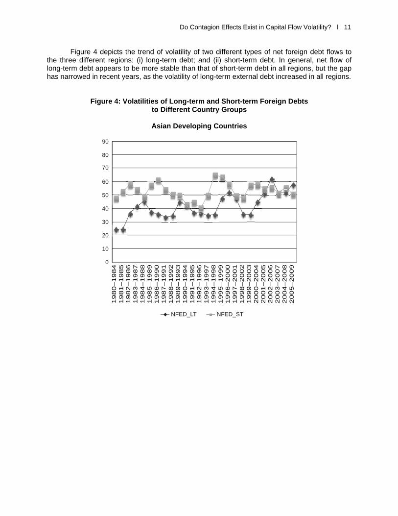
Figure 4 depicts the trend of volatility of two different types of net foreign debt flows to the three different regions: (i) long-term debt; and (ii) short-term debt. In general, net flow of long-term debt appears to be more stable than that of short-term debt in all regions, but the gap has narrowed in recent years, as the volatility of long-term external debt increased in all regions.

Figure 4: Volatilities of Long-term and Short-term Foreign Debts to Different Country Groups

Asian Developing Countries

19

80

–1

98

41

98

1–

19

85

19

82

–1

98

61

98

3–

19

87

19

84

–1

98

81

98

5–

19

89

19

86

–1

99

01

98

7–

19

91

19

88

–1

99

21

98

9–

19

93

19

90

–1

99

41

99

1–

19

95

19

92

–1

99

61

99

3–

19

97

19

94

–1

99

81

99

5–

19

99

19

96

–2

00

01

99

7–

20

01

19

98

–2

00

21

99

9–

20

03

20

00

–2

00

42

00

1–

20

05

20

02

–2

00

62

00

3–

20

07

20

04

–2

00

82

00

5–

20

09

90

80

70

60

50

40

30

20

10

0

NFED_LT NFED_ST


(B) Latin American Developing Countries

(C) Eastern European Developing Countries

Note: NFED_LT and NFED_ST refer to the 5year standard deviation of net flows on long-term external debt and on short-term external debt in % of GDP, respectively.

Source: Calculated by the authors using World Bank’s World Development Indicators-Global Development Finance online database.

19

80

–1

98

41

98

1–

19

85

19

82

–1

98

61

98

3–

19

87

19

84

–1

98

81

98

5–

19

89

19

86

–1

99

01

98

7–

19

91

19

88

–1

99

21

98

9–

19

93

19

90

–1

99

41

99

1–

19

95

19

92

–1

99

61

99

3–

19

97

19

94

–1

99

81

99

5–

19

99

19

96

–2

00

01

99

7–

20

01

19

98

–2

00

21

99

9–

20

03

20

00

–2

00

42

00

1–

20

05

20

02

–2

00

62

00

3–

20

07

20

04

–2

00

82

00

5–

20

09

90

80

70

60

50

40

30

20

10

0

NFED_LT NFED_ST

19

80

–1

98

41

98

1–

19

85

19

82

–1

98

61

98

3–

19

87

19

84

–1

98

81

98

5–

19

89

19

86

–1

99

01

98

7–

19

91

19

88

–1

99

21

98

9–

19

93

19

90

–1

99

41

99

1–

19

95

19

92

–1

99

61

99

3–

19

97

19

94

–1

99

81

99

5–

19

99

19

96

–2

00

01

99

7–

20

01

19

98

–2

00

21

99

9–

20

03

20

00

–2

00

42

00

1–

20

05

20

02

–2

00

62

00

3–

20

07

20

04

–2

00

82

00

5–

20

09

90

80

70

60

50

40

30

20

10

0

NFED_LT NFED_ST


Tables in Appendix 2 provide the estimated volatilities for different types of capital flows into the 50 individual countries included in the sample of the study.

III. EMPIRICAL SPECIFICATION A. The Model This paper constructs a panel data set using the volatility measures obtained in the previous section as the dependent variable. Explanatory variables are grouped in three categories: external variables, policy variables, and control variables. The equation to be estimated is VMit = β0 + EVit β1 + PVit-1 β2 + CVit-1 β3 + εit. (2)

Where VM is a volatility measure of the five different types of capital inflows, EV is a vector of external variables, PV is a vector of policy variables, and CV is a vector of control variables. β is a vector of unknown coefficients and εit is an error term. As will be explained, except for external variables, all other explanatory variables are one-year lagged to minimize endogeneity problem. B. Dependent Variable We use volatility of capital inflows measured by standard deviation of capital flows relative to GDP (drawn from IMF’s IFS database). First, this paper compares the volatilities of the following three types of capital flows:

VFDI : 5-year standard deviation of net foreign direct investment inflows in % of

GDP VFPI: 5-year standard deviation of net portfolio investment inflows in % of GDP VOI: 5-year standard deviation of net other investment inflows in % of GDP Second, the following two definitions of external debt (drawn from World Bank’s WDI-

GDF) online database) will also be used as dependant variables. VED_LT: 5-year standard deviation of net inflows on long-term external debt in %

of GDP VED_ST: 5-year standard deviation of net inflows on short-term external debt in

% of GDP As noted above, we also compute standard deviations over moving window of 3 years to

check the robustness of the empirical results.

C. Explanatory Variables External Variables: The dearth of theory to predict volatility dynamics of capital flows explains a wide spectrum of models and variables used to determine the capital flow volatility. As the main purpose of this paper as asserted in the introduction is to assess the effects of spillover or contagion in the volatility of capital flows to emerging economies, we construct two separate variables to evaluate the impact of regional and global volatilities on the volatility of capital flows to individual


economies. First, intraregional volatility is constructed as the simple average volatility of capital flows to the neighboring countries in the same region when an individual economy belongs to each of three regional groups—East Asia, Latin America, and Eastern Europe.7 Second, global volatility is constructed as the simple average of volatilities of capital flows to all emerging countries in the sample. Global volatility can be further refined to extra-regional volatilities of capital flows to emerging countries. That is, extra-regional volatility is constructed as the simple average volatility of capital flows to all other emerging countries outside each of the three regional groups.

1. Global Volatility

ALL: Simple average of the world-wide volatilities of net capital inflows to all emerging countries

2. Intraregional Volatility

East_Asia_Intra: Simple average volatility of net capital inflows to other neighboring countries in East Asia

Latin_America_Intra: Simple average volatility of net capital inflows to other neighboring countries in Latin America

East_Europe_Intra: Simple average volatility of net capital inflows to other neighboring countries in Eastern Europe

Extraregional Volatility East_Asia_Extra: Simple average volatility of net capital inflows into other emerging

countries outside East Asia Latin_America_Extra: Simple average volatility of net capital inflows into other emerging

countries outside Latin America East_Europe_Extra: Simple average volatility of net capital inflows into other emerging

countries outside Eastern Europe As contagion can occur in very short-term, the above global and regional volatility

variables enter in regression contemporaneously.

Policy Variables: We also include some policy variables in the regression analysis to assess how these variables are associated with the volatility of capital flows to emerging economies. Four policy variables are considered: financial market openness, institutional quality, macroeconomic stability, and accumulation of foreign exchange reserves.

Financial openness is measured as Chin and Ito’s (2010) financial openness index

which is the extensity of capital controls based on the information from the IMF’s Annual Report

7 The whole sample also includes the developing countries located in Africa, Middle East, South Asia, and the

Pacific, but the average volatility of capital inflows to these countries is not included as these countries do not reveal regional identity as compared with Asia, Latin America, and Eastern Europe. See Appendix 1 for the list of the countries in each regional group.


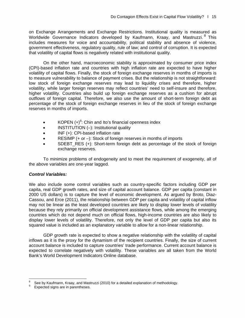
on Exchange Arrangements and Exchange Restrictions. Institutional quality is measured as Worldwide Governance Indicators developed by Kaufmann, Kraay, and Mastruzzi. 8 This includes measures for voice and accountability, political stability and absence of violence, government effectiveness, regulatory quality, rule of law; and control of corruption. It is expected that volatility of capital flows is negatively related with institutional quality.

On the other hand, macroeconomic stability is approximated by consumer price index

(CPI)-based inflation rate and countries with high inflation rate are expected to have higher volatility of capital flows. Finally, the stock of foreign exchange reserves in months of imports is to measure vulnerability to balance of payment crises. But the relationship is not straightforward: low stock of foreign exchange reserves may lead to liquidity crises and therefore, higher volatility, while larger foreign reserves may reflect countries’ need to self-insure and therefore, higher volatility. Countries also build up foreign exchange reserves as a cushion for abrupt outflows of foreign capital. Therefore, we also use the amount of short-term foreign debt as percentage of the stock of foreign exchange reserves in lieu of the stock of foreign exchange reserves in months of imports.

KOPEN (+)9: Chin and Ito’s financial openness index INSTITUTION (–): Institutional quality INF (+): CPI-based inflation rate RESIMP (+ or –): Stock of foreign reserves in months of imports SDEBT_RES (+): Short-term foreign debt as percentage of the stock of foreign

exchange reserves. To minimize problems of endogeneity and to meet the requirement of exogeneity, all of

the above variables are one-year lagged.

Control Variables: We also include some control variables such as country-specific factors including GDP per capita, real GDP growth rates, and size of capital account balance. GDP per capita (constant in 2000 US dollars) is to capture the level of economic development. As argued by Broto, Diaz-Cassou, and Erce (2011), the relationship between GDP per capita and volatility of capital inflow may not be linear as the least developed countries are likely to display lower levels of volatility because they rely primarily on official development assistance flows, while among the emerging countries which do not depend much on official flows, high-income countries are also likely to display lower levels of volatility. Therefore, not only the level of GDP per capita but also its squared value is included as an explanatory variable to allow for a non-linear relationship.

GDP growth rate is expected to show a negative relationship with the volatility of capital

inflows as it is the proxy for the dynamism of the recipient countries. Finally, the size of current account balance is included to capture countries’ trade performance. Current account balance is expected to correlate negatively with volatility. These variables are all taken from the World Bank’s World Development Indicators Online database.

8 See by Kaufmann, Kraay, and Mastruzzi (2010) for a detailed explanation of methodology. 9 Expected signs are in parentheses.


GDP_PC (+): log of GDP per capita (constant in 2000 US dollars) GDP_PC_SQ (–) : GDP_PC squared PGDP (–): Change in GDP_PC (i.e., growth rate): CABL (+): Current account balance (% of GDP) Similarly to the policy variables, the control variables are also one-year lagged.

D. Specification

As mentioned in the previous section, the standard deviation of a moving window is strongly persistent as it leans on previous periods. That is, the standard deviations using overlapping rolling widows are highly correlated by construction. Therefore, when the standard deviation of capital flows over a rolling widow is used as the dependent variable in a regression analysis, the error term is serially correlated by construction. In order to overcome this drawback, this study utilizes the system GMM estimator for dynamic panel data models of Blundell and Bond (1998).

IV. RESULTS

A. Global Contagion Effects

Table 1a reports the results for the contagion effects of all other emerging countries, the impact of the policies, and the country specific condition. The sample covers the period of 1980–2009. Note that the dependant variable is the standard deviation of inflows of different types of capital as ratio of GDP over the 5-year rolling windows. Columns (1)–(3) report the results for FDI, portfolio investment, and other investments, respectively, when RESIMP is included, while Columns (4)–(6) report the corresponding results when RESIMP is replaced with SDEBT_RES. The estimated value for each moving window is assigned as the volatility of capital flows for the midyear in each rolling window, and as previously noted, except for the external variable, all policy and control variables are one-year lagged.

The estimated results are described here by the type of variables.

Control Variables Before turning to the contagion effect variable, let us first consider the estimates for GDP per capita in Table 1a. Both GPD per capita in its level (GDP_PC) and quadratic term (GDP_PC_SQ) yield statistically significant estimates in Columns (1–(3) but their signs are not consistent and yield insignificant results in Columns (4)–(6). Therefore, the impact of GDP per capita on capital flow volatility does not seem to be robust and consistent.

GDP growth rate (PGDP) reveals negative and significant results for FDI flow volatility

(in Columns 1 and 4) and other investment (in Column 4), suggesting that countries with fast economic growth tend to incur lower FDI inflow volatilities. In contrast, GDP growth rate is positively and significantly associated with portfolio investment flow volatility (in Columns 2 and 5), which is inconsistent with the common wisdom. Size of current account balance (CABL) is found to be consistent with our expectation for FDI and other investments. That is, in the case of FDI and other investments, size of current account balance is negatively correlated with their volatilities.


Table 1a: Determinants of Volatility of Foreign Capital Inflow to Emerging Countries: 5-Year Moving Windows, Full Sample

Full Sample (1980–2009)

VFDI VFPI VOI VFDI VFPI VOI

(1) (2) (3) (4) (5) (6)

Lag of Dep Variable 1.030*** 0.832*** 0.845*** 0.764*** 0.834*** 0.885***

(0.021) (0.021) (0.008) (0.066) (0.035) (0.048)

ALL 0.655*** 0.740*** 0.493*** 0.841*** 0.780*** 0.478***

(0.084) (0.065) (0.038) (0.071) (0.089) (0.094)

KOPEN 0.018 -0.967*** 1.158*** 0.714*** 1.022 –1.400

(0.279) (0.323) (0.357) (0.247) (2.208) (1.166)

INSTITUTION –1.278* –11.116*** –2.413 1.694 3.199 –12.938*

(0.745) (2.492) (2.074) (3.788) (6.806) (7.231)

INF –0.004*** –0.001*** –0.001*** –0.003*** –0.000 –0.001*

(0.000) (0.000) (0.000) (0.000) (0.000) (0.000)

RESIMP 0.337*** –0.224*** –0.106

(0.070) (0.080) (0.195)

SDEBT_RES 0.001*** 0.007*** 0.000***

(0.000) (0.001) (0.000)

GDP_PC –12.370*** 42.936*** 46.011*** 15.234 40.606 0.064

(3.898) (12.366) (11.575) (19.574) (24.970) (39.441)

GDP_PC_SQ 0.875*** –2.656*** –2.983*** –1.215 –2.848 0.536

(0.256) (0.861) (0.769) (1.373) (1.752) (2.757)

PGDP –0.127*** 0.164*** –0.141*** –0.163*** 0.272*** –0.083

(0.014) (0.025) (0.039) (0.021) (0.056) (0.080)

CABL –0.060*** –0.056 –0.231*** –0.001 –0.027 –0.375***

(0.019) (0.056) (0.044) (0.028) (0.079) (0.050)

Constant 20.786 –193.997*** –187.592*** –57.902 –169.597* –50.603

(15.632) (44.367) (42.449) (68.472) (90.019) (137.452)

Number of observations 957 719 989 722 537 747

Number of groups 49 45 49 35 32 35

Arellano-Bond test

AR(1) –4.475 –3.867 –5.087 –3.462 –3.022 –4.715

p-value 0.000 0.000 0.000 0.000 0.002 0.000

AR(2) 0.358 –2.028 1.478 0.342 –2.023 1.282

p-value 0.720 0.042 0.139 0.750 0.043 0.199

Overidentification test (Sagan)

Chi-squared 39.368 36.963 41.810 25.081 22.366 23.612

p-value 0.777 0.853 0.686 0.996 0.999 0.998

Note: Shown in parentheses are standard errors. ***, **, and * denote one, five, and ten percent level of significance, respectively.


External Variables We find strong contagion effects. The estimates for ALL, or the average value of capital flow volatilities of all emerging countries in the world show positive and significant coefficients in all three equations. That is, capital flows to a developing country become more volatile when capital flows to other developing countries become more volatile. This finding suggests two things. First, a developing country can fall into a difficult situation when other developing countries are experiencing unstable financial turmoil. Second, therefore, there is a need for developing countries to cooperate to reduce the contagion effect of financial turmoil.

Policy Variables As for the policy variables, we find that greater financial market opening (KOPEN) does not lead to a consistent impact on the volatilities of different types of net capital inflows to developing countries. For example, in the case of other investments, countries with greater degree of financial market openness appear to suffer from greater degree of capital volatility, while in the case of portfolio investment, countries with greater degree of financial market openness tend to enjoy lower degree of volatilities of capital inflows. However, when we control for the effect of reserves in relation to short-term debt levels, financial openness has a significant and positive effect only on foreign direct investment flow volatility. This finding is similar to earlier findings [Neumann, Penl, and Tanku (2009); and Mercado and Park (2011)] that financial openness affects different types of capital flows differently. Interestingly, these studies also find that financial openness reduces volatility of portfolio investment flows, while it may increase the volatility of FDI flows.

Institutional quality (INSTITUTION) appears to have significant and negative effects on

all three types of capital flows (FDI, portfolio, and other investments). Consistent with earlier studies [Broner and Rigobon (2006), IMF (2007), Wei (2011), and Mercado and Park (2011)], this result suggests that better institutional quality is associated with more stable flows. Indeed, this is the only policy variable that reduces the volatility of certain capital flows without increasing that of others.

The INF is negative and significant for all three types of capital flows, suggesting that

countries with high inflation rates tend to have lower capital inflow volatility, which is at odds with some earlier findings. Broto, Diaz-Cassou, and Erce (2011) argue that investors might view domestic inflation as a signal of macroeconomic mismanagement in emerging economies, hence inducing an increase in the volatility of capital flows. But Mercado and Park (2011) find no significant effect of inflation on the size and volatility of capital inflows. In any case, this result is puzzling and deserves further investigation in the future studies.

Lastly, RESIMP enters with positive and significant coefficient in the case of FDI, but

with negative and significant coefficients in the case of portfolio investment. On the other hand, SDEBT_RES has a significantly positive effect on all three types of capital flows. While the level of foreign exchange reserves, per se, may not have universal impact on the volatilities of different types of capital flows, its adequacy in relation to the level of short-term debt seems to have a clear implication on capital flow volatility. For example, large short-term debt relative to the level of foreign exchange reserves suggests imprudence in fiscal management, hence increasing the volatility of capital flows.


Table 1b reports the corresponding results for long-term and short-term external debt. Per capita GDP in the level term appears to have a negative influence on the volatilities of long- and short-term debts while its quadratic term seems to have a positive one, although most of these coefficients are insignificant except for the level of per capita GDP on the volatility of long-term debt flows in equation (2). The results suggest high-income economies have generally low volatility of external debt flows to a certain extent, although there is no significant evidence for non-linearity of the relationship. Indeed, high-income economies with relatively healthy credit ratings may be able to attract more stable (and long-term) debt flows.

Table 1b: Determinants of Volatility of Foreign Capital Inflow to Emerging Countries:

5-Year Moving Windows, Full Sample (with Short-term Debt)

Full Sample (1980–2009)VED_LT VED_ST VED_LT VED_ST

(1) (2) (3) (4) Lag of Dep Variable 0.815*** 0.512*** 0.940*** 0.526***

(0.091) (0.065) (0.036) (0.063) ALL 0.025 0.951*** –0.053 0.959***

(0.134) (0.075) (0.094) (0.076) KOPEN –3.511* 0.906 –0.045 0.798

(1.863) (1.455) (1.033) (1.480) INSTITUTION 3.453 6.310 0.384 6.489

(7.563) (6.124) (2.742) (7.083) INF –0.002*** 0.002*** –0.002*** 0.002***

(0.000) (0.001) (0.000) (0.001) RESIMP –0.832** 0.369

(0.379) (0.609) SDEBT_RES –0.001*** 0.000***

(0.000) (0.000) GDP_PC –1.612 –58.089 –38.418* –26.420

(48.350) (62.466) (22.663) (55.768) GDP_PC_SQ 0.378 3.374 2.469 1.359

(3.534) (4.078) (1.553) (3.650) PGDP –0.105** 0.032 –0.092** 0.035

(0.049) (0.051) (0.041) (0.052) CABL 0.179** 0.147* 0.005 0.183***

(0.083) (0.086) (0.060) (0.050) Constant 4.891 215.107 152.265* 93.804

(162.275) (236.819) (83.138) (212.411) Number of observations 757 709 753 709 Number of groups 35 35 35 35 Arellano-Bond test AR(1) –4.050 –4.205 –3.880 –4.373 p-value 0.000 0.000 0.000 0.000 AR(2) 0.001 –0.929 0.276 –0.834 p-value 0.999 0.353 0.782 0.404 Overidentification test (Sagan)

Chi-squared 15.830 27.399 18.637 29.112 p-value 0.996 0.999 1.000 0.981



Among the control variables, only the CABL is found to have a relatively consistent and significant relationship with the volatilities of both long-term and short-term external debt flows. However, the finding suggests that higher CABL is positively related to higher volatility of external debt flows. This finding is not only at odds with our expectation but also different from the previous results for the volatilities of other types of capital flows. This is also puzzling and requires further investigation in future studies.

We find significant global contagion effect on the volatility of short-term external debt

flows (Columns 2 and 4). That is, short-term debt flows to a developing country can become more volatile when short-term external debt flows to other developing countries become more volatile. In contrast, we find no significant global contagion effect on the volatility of long-term external debt flows.

As for the policy variables, KOPEN is negatively associated with the volatility of long-

term external debt flows. INSTITUTION appears to have no significant effect on the volatilities of both short- and long-term external debt flows. Unlike the significant effects on other types of capital flows, this result may reflect that debt financing has relatively more legal and institutional protection, such as creditor rights.

INF appears to have a significantly negative effect on long-term external debt volatility

but a significantly positive effect on short-term external debt volatility. High inflation rates would discourage long-term external debt inflows, affecting their volatility negatively. On the other hand, countries with high inflation rates may offer higher returns on short-term debts, which could increase short-term debt inflow and its volatility.

Finally, the RESIMP has a significant and negative effect on the volatility of long-term

debt flows. SDEBT_RES has a significant and negative effect on long-term external debt volatility and a significant and positive effect on short-term volatility.

B. Intraregional versus Extra-regional Contagion Effects

We divided the contagion effect into intraregional contagion effects and extra-regional contagion effects. Tables 2a and 2b report these contagion effects for the volatilities of the three types of capital inflows and of two different types of external debt inflows to the regions of East Asia, Latin America, and Eastern Europe.


Table 2a: Regional Contagion Effects on Volatility of Foreign Capital Inflow: 5-Year Moving Windows, Full Sample


VFDI VFPI VOI

(1) (2) (3) (4) (5) (6)

Lag of Dep Variable 1.112*** 1.086*** 0.877*** 0.879*** 0.822*** 0.837*** (0.038) (0.030) (0.013) (0.016) (0.027) (0.013)

East_Asia_Intra 0.098* 0.203*** 0.162*** (0.052) (0.037) (0.055)

Latin_America_Intra –0.004 0.125** 0.325*** (0.044) (0.049) (0.046)

East_Europe_Intra 0.035 0.162*** 0.341*** (0.046) (0.060) (0.051)

East_Asia_Extra –0.024 0.196*** –0.119* (0.046) (0.072) (0.064)

Latin_America_Extra –0.184*** 0.158** 0.063 (0.040) (0.076) (0.076)

East_Europe_Extra –0.151*** –0.057 –0.002 (0.045) (0.069) (0.064)

KOPEN –0.395 –0.135 –0.746 –1.053 1.435* 0.356 (0.334) (0.490) (0.732) (0.766) (0.804) (0.699)

INSTITUTION –2.394 0.761 –13.570*** –11.079*** –3.132 –5.333* (1.706) (1.093) (3.035) (3.607) (2.424) (3.067)

INF –0.005*** –0.004*** –0.002*** –0.003*** –0.001*** –0.001*** (0.000) (0.000) (0.000) (0.000) (0.000) (0.000)

RESIMP 0.283*** 0.056 0.158 –0.115 –0.172 –0.138 (0.077) (0.064) (0.313) (0.139) (0.107) (0.167)

GDP_PC –16.011 –6.121 0.883 –13.190 11.873 36.207*** (10.283) (7.674) (12.720) (21.744) (19.883) (11.658)

GDP_PC_SQ 1.133* 0.453 0.104 1.110 –0.890 –2.260*** (0.680) (0.501) (0.898) (1.467) (1.380) (0.821)

PGDP –0.115*** –0.091*** 0.116*** 0.098*** –0.038 –0.083 (0.027) (0.017) (0.026) (0.027) (0.077) (0.057)

CABL –0.054*** –0.026 –0.087 –0.175*** –0.165*** –0.224*** (0.017) (0.022) (0.068) (0.057) (0.052) (0.050)

Constant 49.606 19.276 –12.183 37.651 –36.139 –132.507*** (37.137) (29.242) (42.411) (77.262) (69.588) (39.648)

Number of observations 957 957 713 719 989 989 Number of groups 49 49 45 45 49 49

Arellano-Bond test AR(1) –4.377 –4.533 –3.907 –3.781 –5.151 –5.093 p-value 0.000 0.000 0.000 0.000 0.000 0.000 AR(2) –0.429 –0.482 –1.899 –2.040 1.592 1.407 p-value 0.668 0.629 0.057 0.041 0.111 0.159 Overidentification test (Sagan) Chi-squared 34.924 36.225 38.817 36.440 40.233 40.852 p-value 0.903 0.873 0.796 0.867 0.748 0.723



Table 2b: Regional Contagion Effects on Volatility of Foreign Capital Inflow: 5-Year Moving Windows, Full Sample


VED_LT VED_LT VED_ST VED_ST (1) (2) (3) (4)

Lag of Dep Variable 0.853*** 0.852*** 0.606*** 0.190 (0.109) (0.084) (0.046) (0.130)

East_Asia_Intra 0.058 0.499** (0.061) (0.243)

Latin_America_Intra 0.188 0.500** (0.206) (0.237)

East_Europe_Intra 0.282*** 0.042 (0.094) (0.236)

East_Asia_Extra –0.415* 0.970*** (0.223) (0.277)

Latin_America_Extra –0.199 0.848*** (0.170) (0.276)

East_Europe_Extra –0.486 –0.553*** (0.311) (0.112)

KOPEN 1.819 –5.242*** –0.534 0.132 (1.704) (1.689) (1.542) (1.848)

INSTITUTION 15.366* –4.206 0.865 –26.179*** (9.003) (5.027) (8.863) (9.533)

INF –0.002*** –0.001*** 0.003*** 0.001* (0.000) (0.000) (0.001) (0.001)

RESIMP –0.336 –0.161 0.710 –0.419 (0.596) (0.358) (1.000) (0.793)

GDP_PC –6.301 75.156 –42.448 –302.434** (104.509) (56.044) (79.273) (129.209)

GDP_PC_SQ –0.222 –4.508 2.498 19.105** (6.936) (3.711) (5.436) (8.549)

PGDP –0.093*** –0.064 –0.049 0.001 (0.031) (0.075) (0.073) (0.077)

CABL 0.098 0.107 –0.050 0.051 (0.079) (0.080) (0.143) (0.150)

Constant 68.847 –290.998 171.633 1,181.579** (381.157) (208.097) (278.217) (478.465)

Number of observations 757 757 704 709 Number of groups 35 35 35 35

Arellano-Bond test

AR(1) –3.993 –3.948 –4.352 –1.081 p-value 0.000 0.000 0.000 0.080 AR(2) –0.442 0.130 –0.952 –2.198 p-value 0.658 0.896 0.341 0.028 Overidentification test (Sagan)

Chi-squared 18.030 14.923 26.840 16.408 p-value 1.000 1.000 0.999 1.000

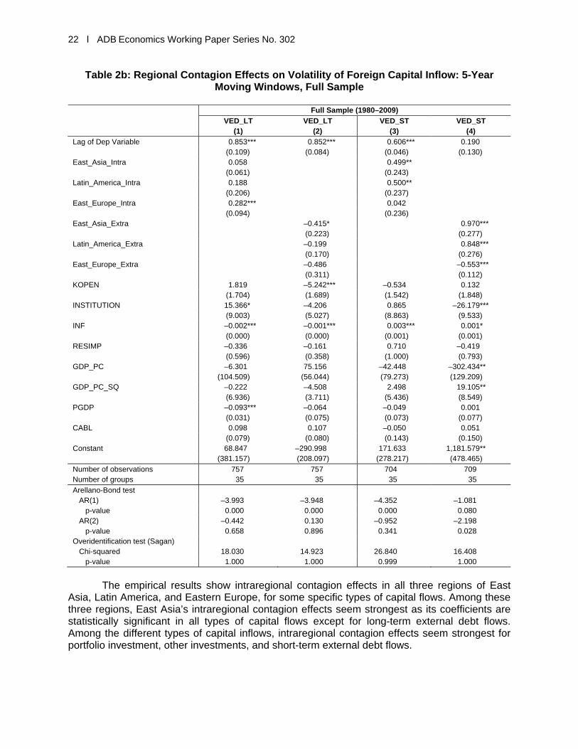
The empirical results show intraregional contagion effects in all three regions of East

Asia, Latin America, and Eastern Europe, for some specific types of capital flows. Among these three regions, East Asia’s intraregional contagion effects seem strongest as its coefficients are statistically significant in all types of capital flows except for long-term external debt flows. Among the different types of capital inflows, intraregional contagion effects seem strongest for portfolio investment, other investments, and short-term external debt flows.


On the other hand, extra-regional contagion effects are observed only for portfolio investment flows and short-term external debt flows to East Asian and Latin American countries. In some cases, the coefficients for extra-regional contagion effects are negative. Strong intraregional contagion effects may reflect the investors’ herding behavior perhaps due to their perception of similarities of these economies and therefore, regional policy coordination may be an important element in designing a policy framework to manage capital inflows.

C. Results for Sub-sample Period: 1995–2009

Broto, Diaz-Cassou, and Erce (2011) argued that “since 2000, global factors beyond the control of emerging economies have become increasingly significant relative to country-specific drivers” (p.1). As an attempt to test their argument, we also estimate the global and regional contagion effects for the sub-sample period of 1995–2009 separately from the whole sample period of 1980 –2009. Note that we cover the sub-sample period from 1995 instead of 2000 in order to allow for more variation.

Tables 3a, 3b, 4a, and 4b report the corresponding results for the sub-sample period of

1995–2009. Here we focus on the contagion effects. During the sub-sample period, the size of ALL, the average of capital flow volatilities, is larger than that of the whole period in most types of capital flows, suggesting that global contagion effects have gained weight. Policymakers in developing countries may face greater challenges of ensuring financial stability in recent years as capital flow volatility in their economies seems to be more easily influenced by the volatility of capital flows to all other developing countries.

Tables 4a and 4b generally confirm that intraregional contagion effects remain strong.

However, the size of coefficients varies depending upon the types of capital and the regions. A noticeable finding is that intraregional contagion effect seems generally stronger than extra-regional contagion effect for most types of capital flows and for most regions, with the exception of volatility of FDI flows to emerging Asia. In emerging Asia, intraregional contagion is strong for FDI and foreign portfolio investment (FPI) low volatility. But in both Latin America and Eastern Europe, volatilities of FPI and other investment flows are more exposed to intraregional contagion than that of FDI flows. In terms of debt flows, intraregional contagion is significant for both long-term and short-term debt flows in emerging Asia. However, in Latin America, intraregional contagion is significant and negative only for short-term debt flow volatility, while it is significant and positive only for long-term flows in Eastern Europe.

Institutional quality continues to have a strong, negative relationship with the volatilities

of other investments and short-term external debt inflows. This result is quite impressive as it is difficult to believe that institutional quality changed dramatically for many countries in the sample during this shorter period of the sub-sample. There is a strong need for developing countries to enhance their institutional quality while the international community needs to find ways to reduce the contagion effect of financial turmoil among developing countries.

Again, other policy variables have differential impacts on the volatilities of capital inflow

depending on the different types and the different regions/economies. Institutional quality seems to be the only policy variable that reduces the volatility of certain capital flows without increasing that of others.


Table 3a: Determinants of Volatility of Foreign Capital Inflow to Emerging Countries: 5-Year Moving Windows, Sub-sample

Sub-sample (1995–2009)

VFDI VFPI VOI VFDI VFPI VOI (1) (2) (3) (4) (5) (6)

Lag of Dep Variable 0.907*** 0.939*** 0.865*** 0.899*** 0.858*** 0.956*** (0.041) (0.049) (0.044) (0.036) (0.033) (0.028)

ALL 0.705*** 0.730*** 1.071*** 0.897*** 1.110*** 0.883*** (0.214) (0.189) (0.298) (0.201) (0.165) (0.284)

KOPEN 0.352 –0.535 3.498*** 1.043** 0.829* 2.163** (0.591) (0.837) (1.160) (0.464) (0.447) (1.100)

INSTITUTION –2.224 –6.213 –6.576** 0.603 1.715 –4.430* (1.475) (3.817) (3.265) (1.685) (1.873) (2.362)

INF –0.000 0.003** 0.010*** 0.001** 0.010*** 0.016*** (0.001) (0.002) (0.002) (0.001) (0.003) (0.002)

RESIMP 0.243** –0.542** –0.058 (0.105) (0.246) (0.296)

SDEBT_RES –0.012*** –0.008 –0.011 (0.002) (0.013) (0.009)

GDP_PC –18.479** 35.995 48.913** 13.908 66.707*** 33.729 (8.799) (24.052) (22.990) (13.244) (15.214) (31.681)

GDP_PC_SQ 1.217** –2.364 –3.270** –1.050 –4.747*** –2.176 (0.569) (1.617) (1.438) (0.872) (1.084) (2.173)

PGDP –0.015 0.161** 0.155 0.011 0.200*** 0.407*** (0.073) (0.081) (0.159) (0.066) (0.072) (0.114)

CABL –0.116** 0.264*** –0.237** –0.097** 0.094 –0.313*** (0.048) (0.093) (0.101) (0.047) (0.122) (0.070)

Constant 49.925 –161.518* –223.473** –66.591 –273.673 –169.369 (31.321) (89.123) (90.005) (47.511) (56.322) (113.954)

Number of observations 558 490 558 402 354 402 Number of groups 49 45 49 35 32 35

Arellano-Bond test AR(1) –3.925 –4.563 –4.719 –3.361 –4.033 –4.203 p-value 0.000 0.000 0.000 0.000 0.000 0.000 AR(2) 0.004 –1.813 0.647 0.175 –1.701 0.508 p-value 0.997 0.069 0.517 0.861 0.088 0.611 Overidentification test (Sagan) Chi-squared 25.743 22.132 15.721 25.081 23.666 19.340 p-value 0.216 0.391 0.785 0.996 0.309 0.563



Table 3b: Determinants of Volatility of Foreign Capital Inflow to Emerging Countries: 5-Year Moving Windows, Sub-sample (with Short-term Debt)


VED_LT VED_ST VED_LT VED_ST (1) (2) (3) (4)

Lag of Dep Variable 0.878*** 0.663*** 0.834*** 0.648*** (0.032) (0.061) (0.029) (0.055)

ALL 0.390** 1.073*** 0.329* 1.121*** (0.168) (0.101) (0.177) (0.108)

KOPEN 0.784 –0.907 1.460 –1.227* (0.800) (0.673) (0.917) (0.668)

INSTITUTION 0.116 –11.504*** 0.322 –9.316** (2.517) (3.607) (2.345) (4.270)

INF 0.011*** –0.010*** 0.009*** –0.010*** (0.001) (0.003) (0.001) (0.002)

RESIMP 0.041 0.241 (0.156) (0.192)

SDEBT_RES 0.000 –0.033*** (0.008) (0.003)

GDP_PC 0.232 –58.200* 0.602 –45.488 (16.420) (34.917) (17.590) (30.350)

GDP_PC_SQ 0.375 3.497 0.437 2.761 (1.101) (2.322) (1.154) (2.023)

PGDP –0.341*** 0.009 –0.266*** –0.080 (0.101) (0.083) (0.098) (0.078)

CABL –0.153** 0.122 –0.121 0.057 (0.071) (0.098) (0.084) (0.111)

Constant –33.105 189.801 –34.573 138.880 (64.099) (127.336) (69.660) (111.166)

Number of observations 412 396 408 396 Number of groups 35 35 35 35

Arellano-Bond test AR(1) –3.310 –4.342 –3.366 –4.323 p-value 0.000 0.000 0.000 0.000 AR(2) 0.031 –0.563 0.043 –0.204 p-value 0.975 0.573 0.966 0.838 Overidentification test (Sagan) Chi-squared 17.756 23.119 21.789 24.979 p-value 0.664 0.337 0.411 0.248



Table 4a: Regional Contagion Effects on Volatility of Foreign Capital Inflow: 5-Year Moving Windows, Sub-sample


VFDI VFPI VOI

(1) (2) (3) (4) (5) (6)

Lag of Dep Variable 0.944*** 0.925*** 0.900*** 0.848*** 0.834*** 0.893***

(0.060) (0.054) (0.042) (0.038) (0.066) (0.047)

East_Asia_Intra 0.211*** 0.419*** 0.023

(0.082) (0.074) (0.148)

Latin_America_Intra 0.036 0.389*** 0.370***

(0.161) (0.070) (0.117)

East_Europe_Intra 0.110 0.172** 0.410***

(0.106) (0.086) (0.090)

East_Asia_Extra 0.271*** 0.050 –0.255

(0.087) (0.123) (0.206)

Latin_America_Extra –0.036 0.204* 0.008

(0.157) (0.108) (0.182)

East_Europe_Extra 0.183 –0.116 0.044

(0.132) (0.096) (0.108)

KOPEN –0.119 –0.005 –2.077*** –1.331* 3.460*** 2.478**

(0.529) (0.507) (0.724) (0.762) (1.139) (1.191)

INSTITUTION –1.092 –1.524 –0.993 –2.393 –3.942 –10.975***

(1.871) (2.215) (4.444) (4.238) (3.270) (3.995)

INF 0.000 0.001 0.005*** 0.005*** 0.006*** 0.010***

(0.001) (0.001) (0.002) (0.002) (0.002) (0.002)

RESIMP 0.211 0.370*** –0.874*** –0.530* 0.318 0.540*

(0.140) (0.128) (0.216) (0.281) (0.295) (0.313)

GDP_PC –22.714** –10.522 –23.190 28.430 –17.639 –36.034

(10.898) (11.726) (21.321) (31.903) (29.945) (39.926)

GDP_PC_SQ 1.492** 0.719 1.457 –1.887 0.677 2.097

(0.701) (0.782) (1.432) (2.085) (1.833) (2.452)

PGDP –0.068 –0.013 0.163** 0.222*** 0.104 0.267*

(0.077) (0.072) (0.071) (0.074) (0.154) (0.160)

CABL –0.056 –0.127** 0.258*** 0.219** –0.299*** –0.437***

(0.068) (0.054) (0.092) (0.089) (0.095) (0.104)

Constant 83.444** 34.927 90.435 –95.851 91.772 153.085

(41.914) (43.755) (75.808) (116.901) (120.292) (160.160)

Number of observations 558 558 490 490 558 558

Number of groups 49 49 45 45 49 49

Arellano-Bond test

AR(1) –3.840 –3.831 –4.302 –4.252 –4.572 –4.764

p-value 0.000 0.000 0.000 0.000 0.000 0.000

AR(2) 0.016 –0.001 –1.937 –1.782 0.613 0.431

p-value 0.987 0.998 0.052 0.074 0.539 0.666

Overidentification test (Sagan)

Chi-squared 27.917 22.106 29.659 29.098 28.438 34.239

p-value 0.142 0.393 0.099 0.111 0.128 0.034



Table 4b: Regional Contagion Effects on Volatility of Foreign Capital Inflow: 5-Year Moving Windows, Sub-sample


VED_LT VED_LT VED_ST VED_ST (1) (2) (3) (4)

Lag of Dep Variable 0.936*** 0.872*** 0.672*** 0.659*** (0.043) (0.035) (0.070) (0.062)

East_Asia_Intra 0.216*** 0.176** (0.061) (0.074)

Latin_America_Intra 0.070 –0.395** (0.084) (0.154)

East_Europe_Intra 0.489*** 0.108 (0.104) (0.098)

East_Asia_Extra –0.213*** 0.113 (0.077) (0.073)

Latin_America_Extra –0.118 –0.230* (0.147) (0.135)

East_Europe_Extra –0.221 –0.332 (0.179) (0.224)

KOPEN 1.619** 1.034* –0.888* –0.767 (0.717) (0.617) (0.466) (0.529)

INSTITUTION –0.915 1.159 –15.776*** –11.533*** (3.076) (2.795) (4.079) (3.802)

INF 0.011*** 0.011*** –0.006*** –0.004* (0.002) (0.002) (0.002) (0.002)

RESIMP 0.206 0.311* –0.071 –0.365* (0.209) (0.177) (0.207) (0.211)

GDP_PC –27.992 10.000 –94.144*** –43.099* (17.536) (16.312) (35.142) (24.038)

GDP_PC_SQ 2.329** –0.359 6.718*** 2.947* (1.152) (1.078) (2.490) (1.627)

PGDP –0.237*** –0.174* –0.139 –0.078 (0.084) (0.096) (0.100) (0.097)

CABL –0.072 –0.062 –0.038 –0.064 (0.068) (0.068) (0.096) (0.104)

Constant 75.477 –42.918 342.982*** 177.964** (67.797) (61.264) (122.154) (88.064)

Number of observations 412 412 396 396 Number of groups 35 35 35 35 Arellano-Bond test AR(1) –3.158 –3.147 –4.497 –4.313 p-value 0.001 0.001 0.000 0.000 AR(2) –0.133 0.168 –0.521 –0.407 p-value 0.894 0.866 0.602 0.683 Overidentification test (Sagan) Chi-squared 10.920 22.199 28.415 28.172 p-value 0.964 0.388 0.128 0.135


D. Robustness Checks The moving window of “5 years” may not be the right length of window to capture the volatility of capital flow. Therefore, this paper also uses the 3-year moving window as a robustness check. The results are not reported here due to space constraint, but two points are noteworthy. First, global contagion effect continues to prevail in both whole sample and sub-sample, although it does seem to gain weight in the sub-sample period of 1995–2009. Second, a strong intraregional contagion effect is also observed in all three regions for most types of capital inflows

As another robustness check, we also tried a 2-year lag for the explanatory variables

and found similar results.10 The results for global and intraregional contagion effects are robust and strong among all the emerging countries. Similar to our main results, all other explanatory variables (policy and control) again have different effects on capital inflow volatility depending on the type of flow.

V. SUMMARY AND CONCLUSIONS

The purpose of this paper was to assess how the volatility of different types of capital flows to emerging countries is affected by the volatility of capital flows elsewhere as well as other economic and policy factors. For this purpose, this paper suggests adopting more rigorous normalization procedure to the usual standard deviations to provide more accurate measures of capital flow volatility than past studies. The paper estimates volatilities of net capital flows in three different forms (foreign direct investment, foreign portfolio investment, and other investment) as well as net flows on short-term and long-term external debt to individual, regional, and global economies. Then, the volatilities in individual economies have been regressed against the global and regional volatilities as well as a battery of domestic factors.

The empirical results suggest strong and significant contagion effects from intraregional

volatilities in different types of capital flows to emerging economies. The evidence of contagion from regional volatilities implies that there is a strong need for regional policy cooperation to contain the spillover or contagion effects. However, other policy variables have differential and time-varying effects on volatility depending on different types of capital inflow, presenting policy dilemma and challenge to producing coordinated efforts by global and regional policy makers.

10 The results are available from the authors upon request.


Appendix 1: List of Countries in Each Regional Group

East Asia Latin America Eastern Europe Others

HKG Hong Kong, China ARG Argentina BUL Bulgaria BOS Botswana

INO Indonesia BRA Brazil CRO Croatia COTE Cote d'Ivoire

KOR Korea, Rep. of CHI Chile CZE Czech Republic GEO Georgia

MAL Malaysia COL Colombia EST Estonia GHA Ghana

PHI Philippines ECU Ecuador HUN Hungary IND India

PRC People’s Republic of China MEX Mexico LAT Latvia ISR Israel

SIN Singapore PAN Panama LIT Lithuania JOR Jordan

TAP Taipei,China PER Peru POL Poland KAZ Kazakhstan

THA Thailand URU Uruguay RUS Russian Federation KEN Kenya

VIE Viet Nam VEN Venezuela SLK Slovak Republic NIG Nigeria

SLV Slovenia OMA Oman

TUR Turkey PAK Pakistan

UKR Ukraine PNG Papua New Guinea

SAF South Africa

SAU Saudi Arabia

SLV Slovenia

SRI Sri Lanka

Source: Authors’ definition.


Appendix 2: Volatilities of Different Types of Capital Inflows to Developing Countries: 5-year Moving Windows

(A) Volatility of Foreign Direct Investment (FDI) Inflows

Year 1980–1984 1985–1989 1990–1994 1995–1999 2000–2004 2005–2009 ARG 24.6 39.7 15.4 31.4 31.0 23.2 BAN 37.7 47.1 36.9 18.5 BOS 37.4 39.8 50.6 26.0 46.8 27.7 BRA 14.0 34.0 28.4 35.8 24.5 19.3 BUL 37.9 38.7 22.1 26.8 CHI 29.3 36.2 24.2 24.8 18.1 17.8 COL 31.0 32.3 18.5 31.2 12.3 20.6 COTE 25.7 31.4 59.2 17.7 20.1 7.7 CRO 34.6 24.0 25.7 CZE 32.3 32.8 32.9 ECU 15.9 32.4 31.6 19.6 43.0 32.7 EST 25.7 23.0 25.5 GEO 28.4 28.2 GHA 38.0 28.7 41.3 23.8 26.4 36.1 HKG 33.4 12.2 HUN 15.6 24.5 42.7 IND 15.9 16.9 26.7 INO 25.3 10.1 65.1 52.5 25.8 ISR 30.2 17.7 28.3 27.5 32.3 30.4 JOR 31.2 40.4 72.1 43.4 32.5 21.6 KAZ 18.0 19.7 29.5 KEN 35.7 35.8 41.1 29.4 37.2 40.0 KOR 35.2 20.8 23.4 37.6 32.0 31.3 LAT 21.9 28.8 39.4 LIT 33.8 29.2 33.9 MAL 22.1 26.9 16.7 17.3 34.2 31.9 MEX 15.2 17.6 25.4 6.9 18.0 16.3 NIG 76.2 35.7 36.8 14.2 12.9 14.5 OMA 23.3 29.7 22.3 24.7 41.6 20.1 PAK 27.1 16.2 11.1 17.3 30.0 PAN 56.5 54.0 26.0 33.2 34.8 23.2 PER 69.0 34.1 43.6 20.7 22.3 17.6 PHI 64.1 38.0 34.2 23.1 37.9 25.4 PNG 21.5 15.3 32.0 36.6 39.2 43.4 POL 23.1 10.7 42.9 15.8 29.4 24.3 PRC 12.7 37.1 10.7 7.6 23.0 RUS 25.4 28.2 25.1 SAF 44.7 53.9 33.6 40.0 37.7 SAU 45.7 87.7 43.8 62.5 38.9 24.3 SIN 20.3 24.1 27.1 21.5 25.8 32.2 SLK 25.4 36.7 SLV 26.7 36.2 53.0 SRI 23.5 26.3 31.1 32.3 6.2 23.1 TAP 23.1 22.3 33.9 39.9 35.4 THA 19.8 36.1 24.9 36.0 16.6 26.5 TUR 32.9 34.2 13.9 9.5 31.8 25.9 UKR 22.8 17.8 20.7 URU 17.8 27.5 17.4 VEN 37.3 38.4 33.2 32.4 31.9 56.8 VIE 6.2 30.0

Data: 5-year standard deviation of foreign direct investment calculated by the authors using the IMF’s International Financial Statistics online database.

Source: Authors’ calculation.


(B) Volatility of Foreign Portfolio Investment (FPI) Inflows

Year 1980–1984 1985–1989 1990–1994 1995–1999 2000–2004 2005–2009

ARG 36.5 26.2 40.5 57.7 37.9 69.2

BAN 42.6 42.1 77.2 37.1

BOS 69.1 55.8 47.1 76.7

BRA 73.6 20.8 39.1 31.3 72.6 43.8

BUL 73.6 45.3 61.9

CHI 29.7 40.9 40.5 46.5

COL 28.4 26.2 47.4 48.0

COTE 22.3 47.5 37.6

CRO 50.9 31.7 68.3

CZE 27.8 32.9 39.2

ECU 41.6 44.8 49.6

EST 40.7 35.8 48.4

GEO 40.7

GHA 38.9 26.5 35.5 34.6 33.5 47.2

HKG 44.2 44.2

HUN 66.0 37.1 54.7

IND 40.7 37.5 52.1

INO 61.6 46.2 90.6 67.0 27.9

ISR 46.3 44.4 50.9 28.5 52.3 23.1

JOR 32.1 41.1

KAZ 45.9 53.5 48.9

KEN 36.3 71.6 39.5

KOR 44.7 50.4 35.1 35.2 26.3 53.4

LAT 41.3 44.5

LIT 41.5 28.0 38.5

MAL 37.1 47.7 46.5 48.4 52.1 62.8

MEX 85.5 71.8 33.1 72.1 61.2 39.2

NIG 46.5 25.9 33.7

OMA 66.0 66.0

PAK 36.4 38.7 54.7 58.7

PAN 75.0 26.5 37.3 67.4 42.2 39.6

PER 68.7 43.5 45.5

PHI 40.2 47.0 47.8 46.1 56.6

PNG

POL 39.3 31.9 50.6

PRC 34.3 43.2 40.7 32.5

RUS 48.4 49.1 69.6

SAF 52.9 35.9 33.5 63.2 48.9

SAU

SIN 38.4 55.9 44.3 42.9 57.9 68.1

SLK 41.3 44.8

SLV 37.5 48.0 39.4

SRI 18.6 27.7 11.5

TAP 48.3 42.2 41.1 30.4 57.3

THA 25.7 43.1 42.2 45.2 66.9 47.1

TUR 37.4 71.5 65.8 47.5

UKR 70.1 40.6 62.2

URU 44.9 27.2 32.9 27.4 32.5 46.2

VEN 43.6 57.8 50.6 80.4

VIE 42.5

Data: 5-year standard deviation of foreign portfolio investment calculated by the authors using the IMF’s International Financial Statistics online database.



(C) Volatility of Other Inflows (OI)

Year 1980–1984 1985–1989 1990–1994 1995–1999 2000–2004 2005–2009

ARG 60.9 46.0 56.6 37.8 40.5 66.2

BAN 16.0 16.9 21.3 13.8 25.3 30.0

BOS 18.9 36.8 29.7 23.3 62.8 48.4

BRA 68.7 16.8 38.6 69.9 40.6 44.3

BUL 37.8 70.5 65.4 39.7 40.8

CHI 71.2 34.2 64.6 34.0 80.6 71.7

COL 22.1 48.0 76.4 49.7 46.0 44.3

COTE 52.3 34.0 35.9 37.5 39.0 77.5

CRO 30.4 36.4 20.4

CZE 40.5 59.2 54.9

ECU 62.3 25.6 64.3 52.9 51.9 59.2

EST 33.3 29.9 48.5

GEO 57.7 34.8

GHA 37.1 34.5 21.0 24.6 51.9 56.3

HKG 76.9 45.5

HUN 28.2 38.1 69.7 66.1 34.5

IND 29.4 16.9 21.9 33.9 35.5 29.2

INO 28.2 54.3 44.9 28.7 68.9

ISR 30.7 51.3 27.8 29.4 48.0 60.0

JOR 21.5 31.0 53.6 75.1 70.9 75.3

KAZ 29.6 41.3 46.3

KEN 22.1 32.3 53.6 43.2 43.7 20.3

KOR 32.9 46.9 41.8 82.9 55.6 55.4

LAT 28.6 24.6 47.6

LIT 29.1 39.5 57.8

MAL 35.8 54.1 48.6 44.3 49.2 53.4

MEX 44.7 49.2 42.8 69.1 43.0 58.6

NIG 69.0 29.4 36.3 70.0 24.7 49.9

OMA 38.0 46.7 76.2 40.6 66.0 41.5

PAK 17.4 28.5 21.7 94.4 28.4

PAN 71.9 46.1 31.8 75.6 47.0 35.0

PER 56.7 20.3 59.2 50.1 49.9 50.6

PHI 49.8 77.1 15.0 51.6 28.7 80.0

PNG 36.0 25.4 54.7 35.4 55.9 68.5

POL 68.1 35.5 43.5 65.8 59.0 42.2

PRC 29.5 65.2 61.6 46.8 44.5

RUS 72.7 55.9 47.1

SAF 46.2 46.4 60.4 72.5 48.9

SAU 62.8 30.1 59.6 62.8 66.9 53.5

SIN 30.3 40.7 56.1 46.2 39.6 37.5

SLK 59.6 59.2

SLV 30.4 25.2 50.2

SRI 22.2 21.6 17.6 32.9 79.2 36.7

TAP 49.3 34.1 50.0 41.1 54.0

THA 20.0 42.4 17.8 76.7 28.4 59.4

TUR 26.4 73.7 64.2 19.8 64.9 49.2

UKR 26.5 47.9 44.7

URU 38.2 54.5 44.8 43.2 54.9 71.0

VEN 61.2 58.1 47.8 59.3 66.5 61.0

VIE 34.4 28.2

Data: 5-year standard deviation of other investment calculated by the authors using the IMF’s International Financial Statistics online database.



(D) Volatility of Net Flows of Long-term External Debt Year 1980–1984 1985–1989 1990–1994 1995–1999 2000–2004 2005–2009 ARG 42.6 43.3 58.4 25.8 61.4 48.2 BAN 16.6 15.0 21.8 22.3 21.0 26.1 BOS 31.3 37.0 74.9 42.6 30.2 45.6 BRA 18.3 69.5 44.6 59.2 55.6 41.4 BUL 21.2 51.3 80.1 34.4 38.4 CHI 19.6 24.4 29.3 32.8 38.9 40.3 COL 15.3 46.0 64.4 39.2 60.6 43.6 COTE 22.3 44.0 23.7 61.1 27.4 41.0 CRO CZE ECU 44.9 24.3 77.5 40.5 45.5 48.0 EST GEO 16.2 38.4 44.6 GHA 25.2 19.9 6.2 27.4 37.8 29.0 HKG HUN IND 16.4 17.6 23.7 44.3 70.6 39.5 INO 23.1 27.0 49.4 78.8 17.1 52.2 ISR JOR 18.5 25.6 49.8 37.1 52.9 46.5 KAZ 25.6 29.4 34.5 KEN 21.9 25.3 58.0 75.1 39.9 60.3 KOR LAT LIT 39.3 49.4 41.3 MAL 26.2 44.8 71.9 24.2 56.0 69.6 MEX 36.1 52.5 37.7 36.2 63.7 76.7 NIG 43.1 75.5 40.0 24.2 26.2 49.9 OMA PAK 29.0 24.4 18.9 30.0 62.6 14.9 PAN 27.7 37.4 29.7 57.8 32.1 43.9 PER 38.5 17.2 40.7 67.4 4.6 64.0 PHI 15.4 39.8 34.9 37.0 41.7 77.7 PNG 35.2 33.9 63.7 57.9 50.5 57.5 POL PRC 17.7 24.4 45.5 76.9 60.0 RUS 40.8 56.7 40.3 SAF 54.9 47.3 52.4 SAU SIN SLK SLV SRI 16.1 25.8 31.1 35.2 29.4 27.7 TAP THA 18.0 48.6 19.5 61.9 36.2 59.0 TUR 27.9 33.0 45.1 40.4 43.1 50.2 UKR 42.5 48.7 45.0 URU 33.6 41.6 58.6 36.1 42.5 56.8 VEN 50.0 49.7 43.2 43.7 44.8 69.1 VIE 41.5 29.0

Data: 5-year standard deviation of net flows on long-term external debt calculated by the authors using World Bank’s World Development Indicators-Global Development Finance online database.



(E) Volatility of Net Flows of Short-term External Debt Year 1980–1984 1985–1989 1990–1994 1995–1999 2000–2004 2005–2009 ARG 64.9 41.8 46.3 43.4 56.9 BAN 57.5 49.6 70.7 51.2 35.4 46.8 BOS 51.9 70.4 72.4 44.0 BRA 66.5 61.7 42.6 65.6 55.4 50.3 BUL 52.2 60.8 58.0 38.0 CHI 74.4 58.1 55.4 57.0 42.3 COL 74.7 47.1 48.7 55.4 66.3 76.0 COTE 64.9 38.4 54.3 58.4 32.4 CRO CZE ECU 75.8 47.1 45.3 52.8 67.7 72.5 EST GEO 44.4 66.4 73.7 GHA 85.9 62.7 35.5 41.0 56.7 51.4 HKG HUN IND 29.4 16.5 54.9 76.8 60.9 39.8 INO 27.1 40.5 46.2 53.3 74.5 62.6 ISR JOR 41.1 64.9 69.5 81.0 91.3 56.2 KAZ 48.6 20.7 49.0 KEN 78.0 63.3 73.5 54.1 84.4 70.7 KOR LAT LIT 42.6 35.0 79.4 MAL 49.2 70.3 51.5 60.7 69.8 45.3 MEX 69.0 54.4 36.7 35.0 45.0 48.2 NIG 47.3 46.8 77.2 75.5 77.6 65.2 OMA PAK 53.2 28.9 55.7 57.6 64.8 PAN 59.2 44.9 PER 76.7 57.5 72.4 60.1 48.4 49.0 PHI 75.4 57.4 58.0 58.9 73.1 79.6 PNG 73.1 57.5 63.4 64.0 73.7 69.3 POL PRC 62.6 24.7 61.8 39.0 47.3 RUS 49.4 47.3 69.1 SAF 52.6 58.1 63.2 SAU SIN SLK SLV SRI 68.8 58.6 50.1 50.9 53.3 TAP THA 38.7 55.7 27.0 78.0 41.3 26.5 TUR 77.0 70.9 64.9 32.6 57.3 72.8 UKR 70.9 43.2 52.7 URU 39.4 65.2 66.7 29.3 49.7 75.9 VEN 60.6 65.3 54.7 65.5 49.6 50.0 VIE 49.3 44.3

Data: 5-year standard deviation of net flows on short-term external debt calculated by the authors using World Bank’s World Development Indicators-Global Development Finance (WDI-GDF) online database


REFERENCES

Alfaro, L., S. Kalemli-Ozcan, and V. Volosovych. 2007. Capital Flows in a Globalized World: the Role of Policies and Institutions. In S. Edwards, ed. Capital Controls and Capital Flows in Emerging Economies: Policies, Practices and Consequences. Chicago, IL: The University of Chicago Press.

Blundell, R., and S. Bond. 1998. Initial Conditions and Moment Restrictions in Dynamic Panel Data Models. Journal of Econometrics, 68. 29–51.

Broner, F. A., and R. Rigobon. 2006. Why are Capital Flows So Much More Volatile in Emerging than in Developed Countries?” In R. J. Caballero, C. Calderon, and L. F. Cespedes, eds., External Vulnerability and Preventive Policies. Santiago: Central Bank of Chile.

Broto, C., J. Diaz-Cassou, A. Erce. 2011. Measuring and Explaining the Volatility of Capital Flows to Emerging Countries. Journal of Banking and Finance, Article in press.

Calvo, S., and C. Reinhart. 1996. Capital Flows to Latin America: Is There Evidence of Contagion Effect?. In Guillermo Calvo, Morris Goldstein, and Eduard Hochreiter, eds., Private Capital Flows to Emerging Markets after the Mexican Crisis. Washington, DC: Institute for International Economics.

Chinn, M., and H. Ito. 2010. The Chinn-Ito Index: A De Jure Measure of Financial Openness. Available at: http://web.pdx.educ/~ito/Chinn-Ito_website.htm

Karolyi, G. A. 2004. Does International Financial Contagion Really Exist?. Journal of Applied Corporate Finance, 16: 136–146.

Dornbusch, R., C. Y. Park, and S. Claessens. 2000. Contagion: Understanding How It Spreads. World Bank Research Observer. Oxford University Press.

Eichengreen, B., A. K. Rose, and C. Wyplosz. 1997. Contagious Currency Crises. NBER WP 5681; CEPR DP 1453, July 1996. Revised in March 1997. Part of this paper was published in the Scandinavian Journal of Economics 98, 1996.

Engle, R., and J. Gonzalo Rangel. 2008. The Spine GARCH Model for Unconditional Volatility and Its Global Macroeconomic Causes. Review of Financial Studies, 21: 1187–1222.

Fischer, S. 1998. Reforming the International Monetary System. Draft paper prepared for the David Finch Lecture, Melbourne, Australia, presented November 9. Available at <http://www.imf.org/external/np/speeches/1998/110998.htm>

International Monetary Fund. 2007. The Quality of Domestic Financial Markets and Capital Inflows. Global Financial Stability Report 2007. Washington, DC: International Monetary Fund.

Ju, J., and S.-J. Wei. 2006. A Solution to Two Paradoxes of International Capital Flows. NBER Working Paper No. 12668. Cambridge, MA: National Bureau of Economic Research. Karolyi, G. A. 2003. Does International Financial Contagion Really Exist? International Finance, 6: 179–199.


Kaufmann, D., A. Kraay, and M. Mastruzzi. 2010. The Worldwide Governance Indicators: A Summary of Methodology, Data and Analytical Issues. World Bank Policy Research.

Levchenko, A., and P. Mauro.2007. Do Some Forms of Financial Flows Help Protect from Sudden Stops? IMF Working Paper No. 06/202. Washington, DC: International Monetary Fund (IMF).

Mercado, R., and C.-Y. Park. 2011. What Drives Different Types of Capital Flow and Their Volatilities in Developing Asia? International Economic Journal 25: 4. 655–680.

Neumann, R. M., R. Penl, and A. Tanku. 2009. Volatility of Capital Flows and Financial Liberalization: Do Specific Flows Respond Differently. International Review of Economics and Finance, 18, 488–501.

Tong, H., and S.-J. Wei. 2009. The Composition Matters: Capital Inflows and Liquidity Crunch During a Global Economic Crisis. NBER Working Paper No. 15207. Cambridge, MA: NBER.

Wei, S.-J., and W. Wu.2001. Negative Alchemy? Corruption, Composition of Capital Flows, and Currency Crises. NBER Working Paper No. 8187. Cambridge, MA: NBER.

Wei, S-J (2011), Not All Financial Integration is Created Equal: The Composition Matters. M. Devereux, P. Lane, C.Y. Park, and S. J. Wei, eds. In The Dynamics of Asian Financial Integration. London and New York; Routledge Studies in the Modern World Economy.

Do Contagion Effects Exist in Capital Flow Volatility?

Hyun-Hoon Lee, Cyn-Young Park , Hyung-suk Byun No. 302 | September 2012


Do Contagion Effects Exist in Capital Flow Volatility?Hyun-Hoon Lee, Cyn-Young Park, and Hyung-suk Byun examine how the volatility of different types of capital flows to emerging countries is affected by the volatility of capital flows elsewhere as well as other economic and policy factors. The authors find strong and significant contagion effects from global and regional volatilities on the volatility of capital flows to developing economies.

About the Asian Development BankADB’s vision is an Asia and Pacific region free of poverty. Its mission is to help its developing member countries reduce poverty and improve the quality of life of their people. Despite the region’s many successes, it remains home to two-thirds of the world’s poor: 1.8 billion people who live on less than $2 a day, with 903 million struggling on less than $1.25 a day. ADB is committed to reducing poverty through inclusive economic growth, environmentally sustainable growth, and regional integration. Based in Manila, ADB is owned by 67 members, including 48 from the region. Its main instruments for helping its developing member countries are policy dialogue, loans, equity investments, guarantees, grants, and technical assistance.

Asian Development Bank6 ADB Avenue, Mandaluyong City1550 Metro Manila, Philippineswww.adb.org/economics

Printed on recycled paper Printed in the Philippines

do contagion effects exist in capital flow volatility? contagion effects exist in capital flow...

Documents