Complex Langevin Simulations of nonzero density QCD

Dénes SextyWuppertal University

Hadrons and Hadron interactions – Long term workshop Kyoto, 4th of March, 2015.

1. Sign problem in lattice QCD2. Complex Langevin equation and gauge cooling

3. Phase diagram of HDQCD 4. kappa and kappa_s expansion 5. Full QCD

Collaborators: Gert Aarts, Erhard Seiler, Ion-Olimpiu Stamatescu Felipe Attanasio, Lorenzo Bongiovanni, Benjamin Jäger, Zoltán Fodor, Sándor Katz

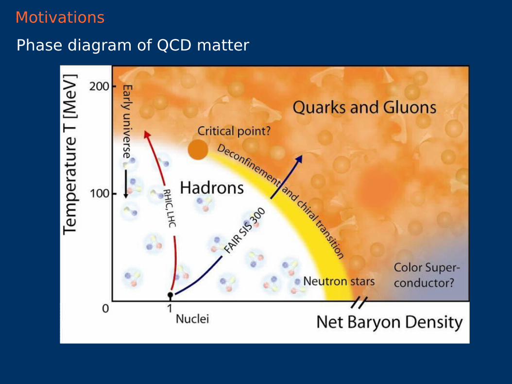
Phase diagram of QCD matter

Motivations

Non-zero chemical potential

Euclidean SU(3) gauge theory with fermions:

Z=∫DAμaD ΨDΨ exp(−SE [Aμ

a]−ΨDE(Aμ

a)Ψ)

For nonzero chemical potential, the fermion determinant is complex

Sign problem Naïve Monte-Carlo breaks down

QCD sign problem

Z=∫DUexp(−SE [U ])det (M(U))

Integrate out fermionic variables, perform lattice discretisation

Aμa ( x , τ) → U μ( x , τ)∈SU (3) link variables

DE (A) → M (U ) fermion matrix

Importance sampling is possibledet (M (U ))>0 →

det (M (U ,−μ ∗ ))=(det (M (U ) ,μ)) ∗

Only the zero density axis is directly accessible to lattice calculations using importance sampling

det (M (U ,μ))∈ℂ for μ>0

Z=∫DUexp(−SE [U ])det (M(U))

Path integral with complex weight

QCD sign problem

⟨F ⟩μ=∫DU e−S E det M (μ)F

∫DU e−S E det M (μ)=∫DU e−S E R

det M (μ)

RF

∫DU e−S E Rdet M (μ)

R

=⟨F det M (μ)/R ⟩R

⟨det M (μ)/R ⟩R

Reweighting

⟨ det M (μ)

R ⟩R

=Z (μ)

Z R

=exp (−VT Δ f (μ , T ))Δ f (μ , T ) =free energy difference

Exponentially small as the volume increases

Reweighting works for large temperatures and small volumes

⟨F ⟩μ → 0 /0

μ/T≈1Sign problem gets hard at

R=det M (μ=0), ∣det M (μ)∣, etc.

(Multi parameter) reweighting

Analytic continuation of results obtained at imaginary

Taylor expansion in

Canonical Ensemble, denstity of states, curvature of critical surface,subsets, fugacity expansion, SU(2) QCD, G2 QCD, dual variables, worldlines, ….

Barbour et. al. '97; Fodor, Katz '02

Most methods going around the problem work only for =B/3T

(μ /T )2

de Forcrand et al. (QCD-TARO) '99; Hart, Laine, Philipsen '00; Gavai and Gupta '03;Allton et al. '05 ; de Forcrand, Philipsen '08,...

Lombardo '00; de Forcrand, Philipsen '02; D'Elia Sanfilippo '09; Cea et. al. '08-,...

μ

Evading the QCD sign problem

Recent revival: Aarts and Stamatescu '08 Bose Gas, Spin model, etc. Aarts '08, Aarts, James '10 Aarts, James '11 Proof of convergence: Aarts, Seiler, Stamatescu '11QCD with heavy quarks: Seiler, Sexty, Stamatescu '12Kappa Expansion: Aarts, Seiler, Sexty, Stamatescu 1408.3770Full QCD with light quarks: Sexty '14

Stochastic quantisation

A Direct Method: Complex Langevin Use analiticity, expand integrals to the complex plane

Stochastic process for x:

d xd

=−∂S∂ x

Gaussian noise

Averages are calculated along the trajectories:

⟨O ⟩=limT→∞

1T∫0

T

O(x (τ))d τ=∫e−S (x)O(x)dx

∫e−S(x)dx

for real action the Langevin method is convergent

Stochastic Quantization Parisi, Wu (1981)

⟨η(τ)⟩=0

Given an action S (x)

⟨η(τ)η(τ ' )⟩=δ(τ−τ ')

Fokker-Planck equation for the probability distribution of P(x):

∂P∂

= ∂∂ x

∂P∂ x

P∂ S∂ x

=−HFPP Real action positive eigenvalues

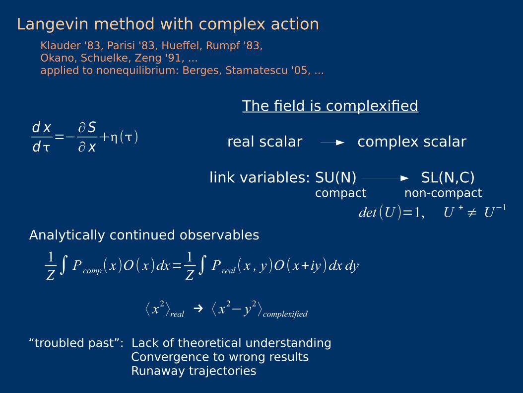
Langevin method with complex action

The field is complexified

real scalar complex scalar

link variables: SU(N) SL(N,C)compact non-compact

Klauder '83, Parisi '83, Hueffel, Rumpf '83,Okano, Schuelke, Zeng '91, ...applied to nonequilibrium: Berges, Stamatescu '05, ...

d xd

=−∂S∂ x

Analytically continued observables

1Z∫ P comp( x )O ( x )dx=

1Z∫ P real ( x , y )O ( x+iy )dx dy

det (U )=1, U + ≠ U−1

⟨ x2⟩real → ⟨ x2− y2⟩complexified

“troubled past”: Lack of theoretical understanding Convergence to wrong results Runaway trajectories

Proof of convergence

S=SW [U μ]+ln Det M (μ) measure has zeroscomplex logarithm has a branch cut meromorphic drift Is it a problem for QCD?

Non-holomorphic action for nonzero density

If there is fast decay

and a holomorphic action

[Aarts, Seiler, Stamatescu (2009) Aarts, James, Seiler, Stamatescu (2011)]

[see also: Mollgaard, Splittorff (2013), Greensite(2014)]

then CLE converges to the correct result

P (x , y )→0 as y→∞

S (x)

(Det M=0)

[QCD and poles: Aarts, Seiler, Sexty, Stamatescu 2014]

Non-real action problems and CLE

1. Real-time physics

2. Theta-Term

[Berges, Stamatescu (2005)][Berges, Borsanyi, Sexty, Stamatescu (2007)][Berges, Sexty (2008)][Anzaki, Fukushima, Hidaka, Oka (2014)][Fukushima, Hayata (2014)]

“Hardest” sign problem eiS M

Studies on Oscillator, pure gauge theory

[Bongiovanni, Aarts, Seiler, Sexty, Stamatescu (2013)+in prep.]

Q=ϵμ νθρF μν F θρ→∑x

q(x)On the lattice

S=F μν Fμν

+iΘϵμ νθρF μν F θρ

Not topologicalCooling is needed bare parameter needs renormalisationΘL

Θ real → complex action, ⟨Q⟩ imaginaryΘ imaginary → real action, ⟨Q⟩ real

Θ imaginary → use real Langevin or HMC Θ real → use complex Langevin

3. Bose gas with non-zero chemical potential

[Aarts (2009)]

4. XY-model, SU(3) Spin model

[Aarts and James (2010-2012)]

6. Random matrix theory

[Mollgaard and Splittorff (2014)]

5. Bose gas in rotating frame

[Hayata and Yamamoto (2014)]

This Talk: QCD with static quarks Hopping expansion of QCD expansion to all orders Full QCD with light quarks

[Seiler, Sexty, Stamatescu (2013)][Aarts, Bongiovanni, Seiler, Sexty, Stamatescu (2013)][Sexty (2014)][Aarts, Seiler, Sexty, Stamatescu (2014)]

S [x ]=σ x2+i λ x

Gaussian Example

σ=1+i λ=20

dd τ

(x+i y )=−2σ(x+iy)−iλ+η

CLE

P (x , y )=e−a(x−x0)2−b( y− y0)

2−c (x−x0)( y− y0)

Gaussian distribution around critical point

∂ S (z)∂ z ]

z0

=0

Measure on real axis

Thimble z=−∂zS (z) Straight lines starting from z0

Measure on thimble

Gauge theories and CLE

Unitarity norm: ∑iTr (U iU i

+ )Distance from SU(N)

Tr (U U + )+Tr (U−1(U−1) + )≥2N

∑ij∣(U U + −1)ij∣

2

link variables: SU(N) SL(N,C)compact non-compact

det (U )=1, U + ≠ U−1

Gauge degrees of freedom also complexify

Infinite volume of irrelevant, unphysical configurations

Process leaves the SU(N) manifold exponentially fast already at μ≪1

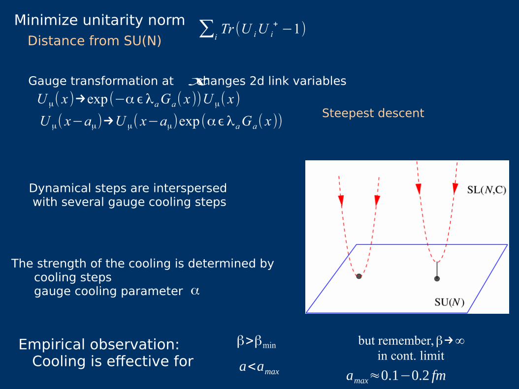
U μ( x−aμ)→U μ( x−aμ)exp(αϵλaGa( x ))

Gauge transformation at changes 2d link variables

U μ( x )→exp(−α ϵλaGa( x ))U μ( x )

Dynamical steps are interspersed with several gauge cooling steps

The strength of the cooling is determined by cooling steps gauge cooling parameter

x

α

Empirical observation: Cooling is effective for

β>βmin but remember,β→∞in cont. limit

a<amax

Minimize unitarity norm ∑iTr (U iU i

+ −1)Distance from SU(N)

Steepest descent

amax≈0.1−0.2 fm

Smaller cooling

excursions into complexified manifold

“Skirt” develops

small skirt gives correct result

The effect of gaugecooling

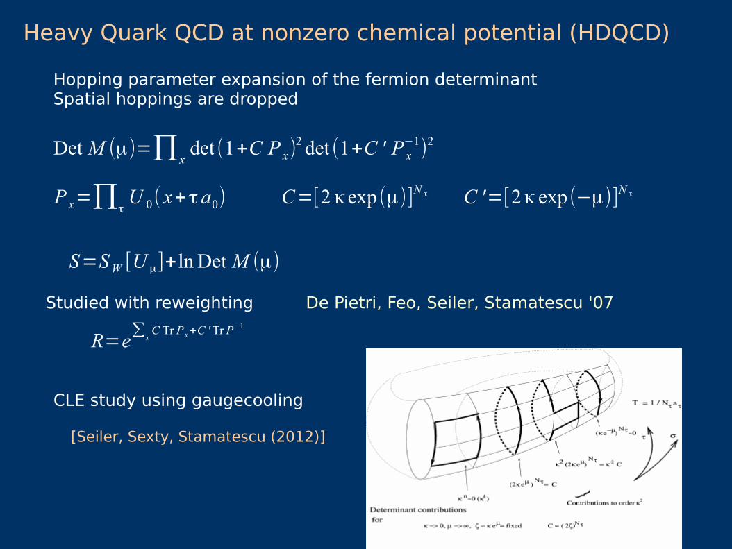
Heavy Quark QCD at nonzero chemical potential (HDQCD)

Det M (μ)=∏xdet (1+C P x)

2 det (1+C ' P x−1)2

P x=∏τU 0( x+τa0) C=[2 κexp(μ)]N τ C '=[2 κexp(−μ)]N τ

Hopping parameter expansion of the fermion determinantSpatial hoppings are dropped

S=SW [U μ]+ln Det M (μ)

Studied with reweighting De Pietri, Feo, Seiler, Stamatescu '07

CLE study using gaugecooling

[Seiler, Sexty, Stamatescu (2012)]

R=e∑

xC Tr Px+C ' Tr P−1

Gauge cooling stabilizes the distribution SU(3) manifold instable even at μ=0

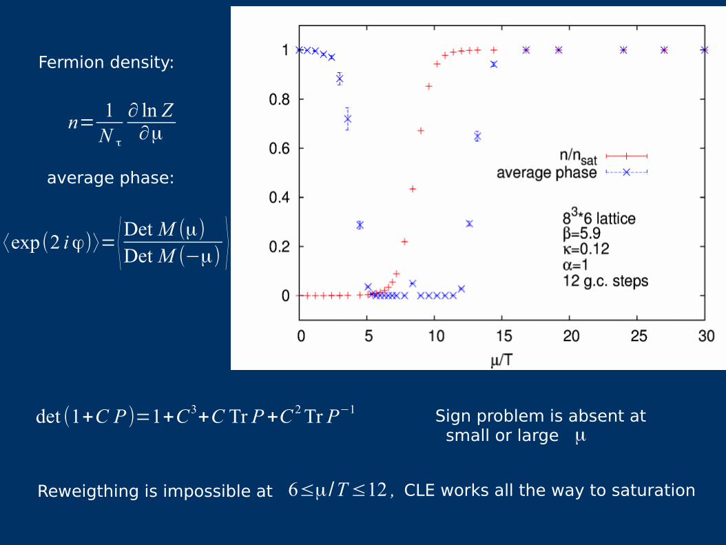
average phase:

⟨exp(2 iϕ)⟩= ⟨ Det M (μ)

Det M (−μ) ⟩

Reweigthing is impossible at 6≤μ/T≤12 , CLE works all the way to saturation

Fermion density:

n=1N τ

∂ ln Z∂μ

det (1+C P )=1+C3+C Tr P+C 2 Tr P−1 Sign problem is absent at small or large μ

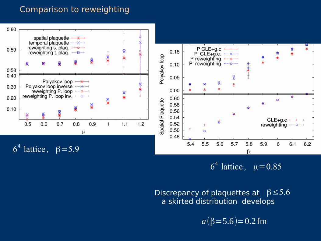
Comparison to reweighting

64 lattice , μ=0.85

Discrepancy of plaquettes at a skirted distribution develops

β≤5.6

64 lattice , β=5.9

a(β=5.6)=0.2 fm

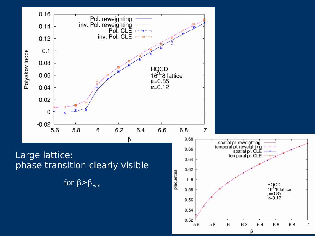
Large lattice: phase transition clearly visible

for β>βmin

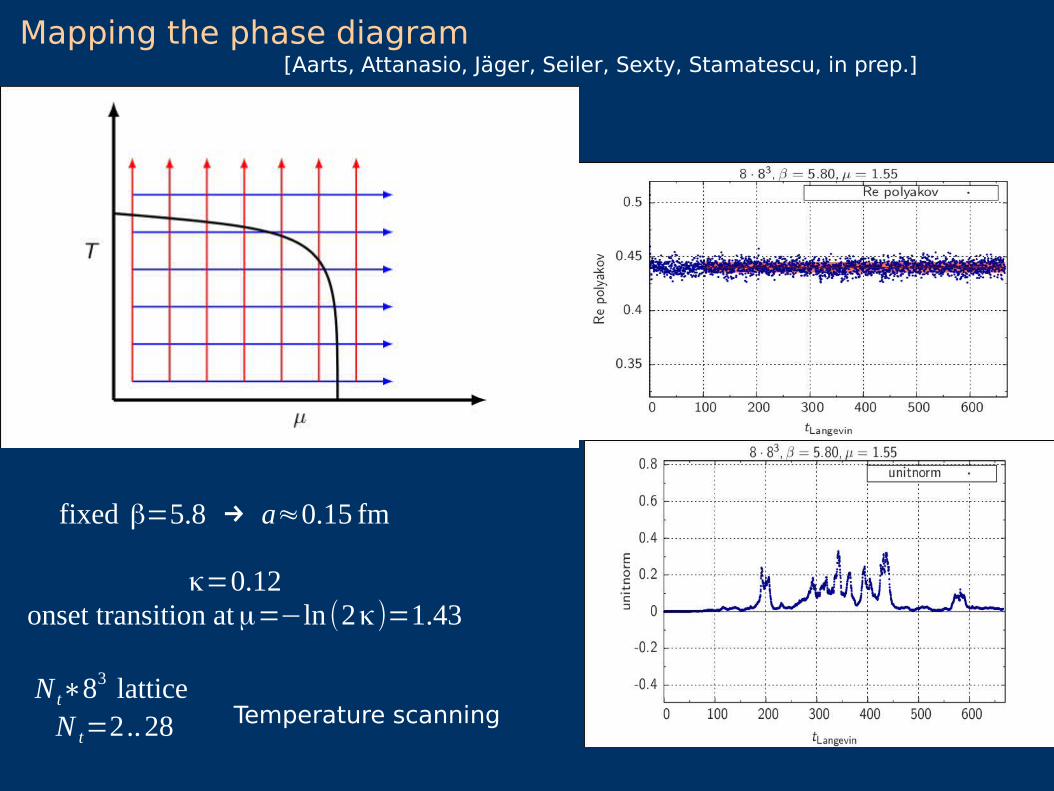
Mapping the phase diagram

fixed β=5.8 → a≈0.15 fm

κ=0.12 onset transition at μ=−ln (2κ)=1.43

N t∗83 lattice N t=2..28 Temperature scanning

[Aarts, Attanasio, Jäger, Seiler, Sexty, Stamatescu, in prep.]

Exploring the phase diagram of HDQCD

Onset in fermionic density Silver blaze phenomenon

Polyakov loop Transition to deconfined state

β=5.8 κ=0.12 N f=2 N t=2. ..24

Polyakov loop susceptibility

Hint of first order deconfinement and first order onset transition

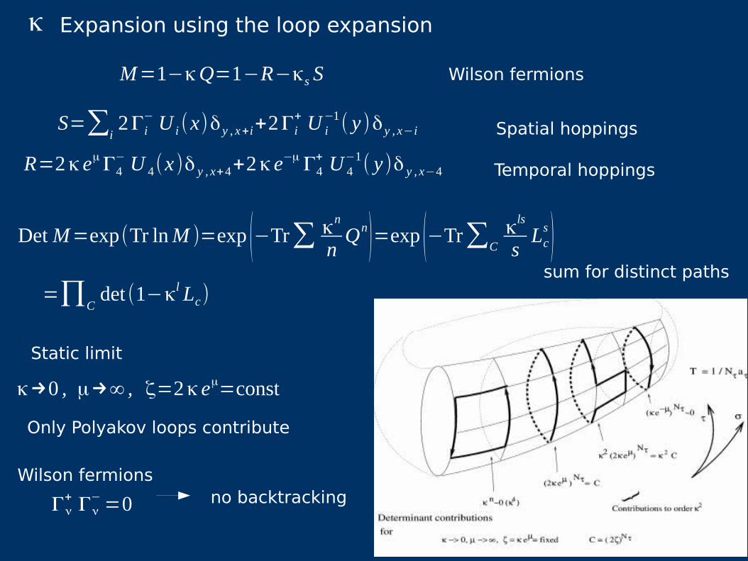
Expansion using the loop expansion κ

M=1−κQ=1−R−κs S

R=2 κ eμ Γ4− U 4(x )δ y , x+4+2 κ e−μ Γ4

+ U 4−1( y)δ y , x−4

S=∑i2Γi

− U i (x)δ y , x+i+2Γi+ U i

−1( y )δ y , x−i Spatial hoppings

Temporal hoppings

Det M=exp(Tr lnM )=exp (−Tr∑ κn

nQn)=exp (−Tr∑C

κls

sLcs )sum for distinct paths

=∏Cdet (1−κl Lc)

Static limit

κ→0 , μ→∞ , ζ=2 κ eμ=const

Only Polyakov loops contribute

Wilson fermions

Γν+ Γν

− =0 no backtracking

Wilson fermions

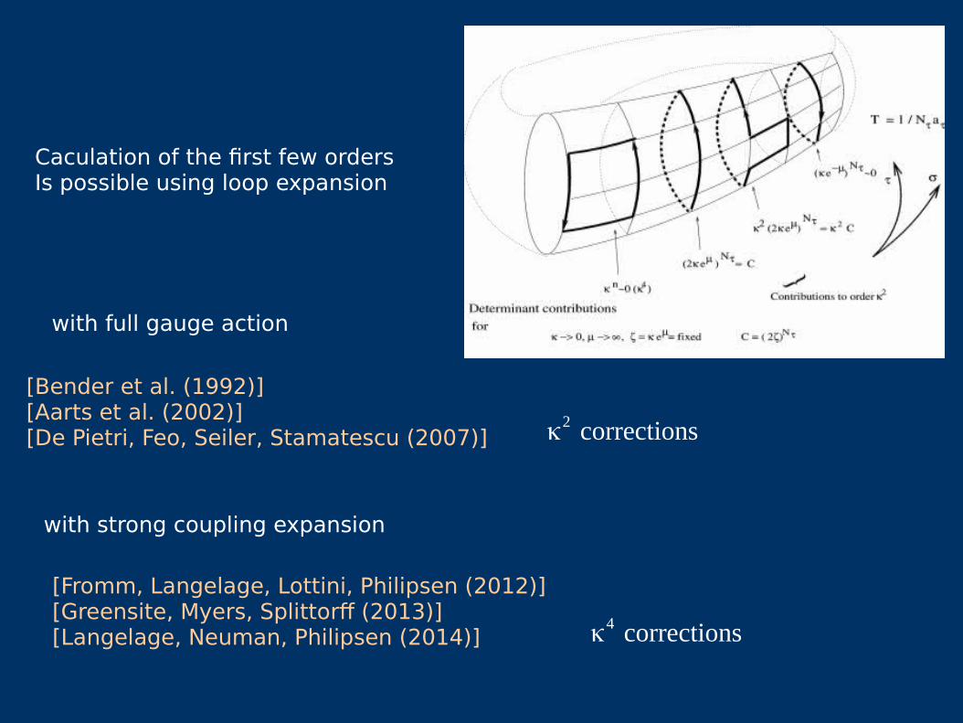
Caculation of the first few orders Is possible using loop expansion

with full gauge action

[Bender et al. (1992)][Aarts et al. (2002)][De Pietri, Feo, Seiler, Stamatescu (2007)]

with strong coupling expansion

[Fromm, Langelage, Lottini, Philipsen (2012)][Greensite, Myers, Splittorff (2013)][Langelage, Neuman, Philipsen (2014)] κ4 corrections

κ2 corrections

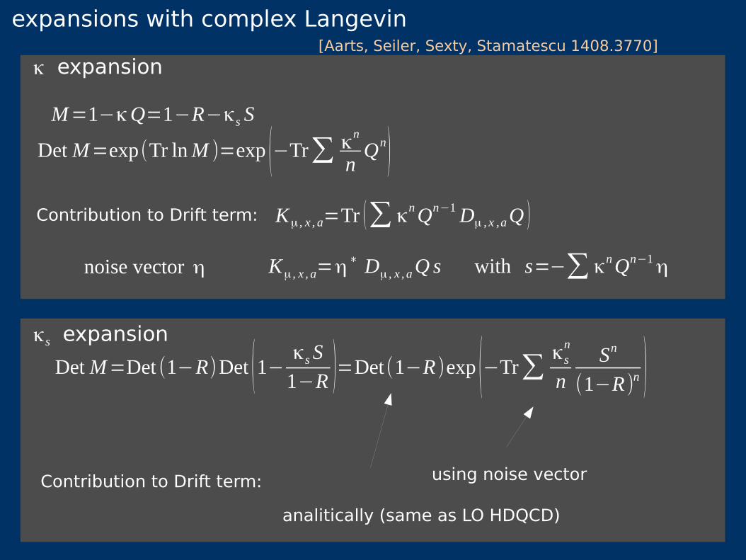
expansions with complex Langevin

M=1−κQ=1−R−κs S

Det M=Det (1−R)Det (1−κsS

1−R )=Det (1−R )exp (−Tr∑κsn

nSn

(1−R )n )

Contribution to Drift term:

Kμ , x , a=Tr (∑ κnQn−1Dμ , x ,aQ )

noise vector η Kμ , x , a=η∗ Dμ , x , aQ s with s=−∑ κnQn−1 η

Det M=exp(Tr lnM )=exp (−Tr∑ κn

nQn)

Contribution to Drift term:

analitically (same as LO HDQCD)

using noise vector

expansionκs

expansionκ[Aarts, Seiler, Sexty, Stamatescu 1408.3770]

Det M=Det (1−R)Det (1−κsS

1−R )=Det (1−R )exp (−Tr∑κsn

nSn

(1−R )n )

Det M=exp(Tr lnM )=exp (−Tr∑ κn

nQn)

expansionκs

expansionκ

Numerical cost: N multiplications with S and (1−R)−1

Numerical cost: N multiplications with Q

Q=R+κS with R + ∝eμbad convergence at high μ

better convergence propertiesTemporal part analytically

Calculation of high orders of corrections is easyExplicit check of the convergence to full QCD

No poles!

Convergence to full QCD with no poles non-holomorphicity of the QCD action is not a problem

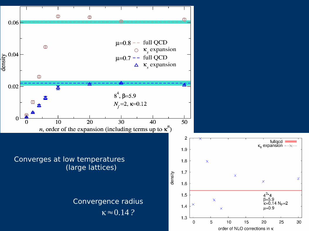
Converges at low temperatures (large lattices)

Convergence radius

κ≈0.14?

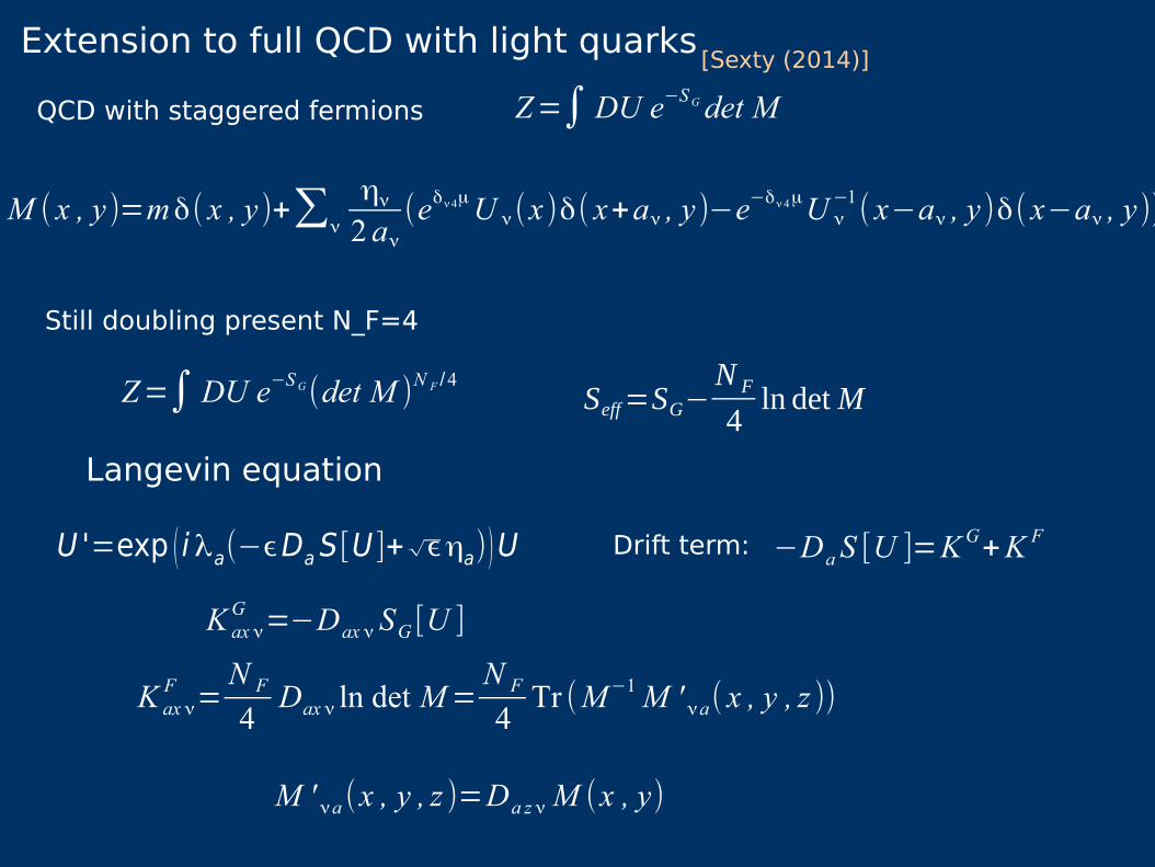
QCD with staggered fermions

M ( x , y )=mδ( x , y )+∑ν

ην

2 aν

(eδν4μU ν (x )δ( x+aν , y )−e−δν 4μU ν

−1( x−aν , y )δ( x−aν , y))

Still doubling present N_F=4

Langevin equation

Z=∫DU e−S G(det M )N F /4

U'=exp ( iλa(−ϵDaS[U ]+√ϵηa))U

Z=∫DU e−S G det M

K ax νF =

N F

4Dax ν ln det M=

N F

4Tr (M−1M ' νa( x , y , z ))

K ax νG =−Dax ν SG [U ]

M ' νa (x , y , z )=Da z νM (x , y)

Extension to full QCD with light quarks[Sexty (2014)]

−DaS [U ]=KG+K FDrift term:

Seff=SG−N F

4ln det M

QCD with fermions Z=∫DU e−S G det M

K ax νF =

N F

4Dax ν ln det M=

N F

4Tr (M−1M ' νa( x , y , z ))

Extension to full QCD with light quarks[Sexty (2014)]

Additional drift term from determinant

Noisy estimator with one noise vector Main cost of the simulation: CG inversion

Unimproved staggered and Wilson fermions

Heavy quarks: compare to HDQCDLight quarks: compare to reweighting

Inversion cost highly dependent on chemical potentialEigenvalues not bounded from below by the mass (similarly to isospin chemical potential theory)

Zero chemical potential

Cooling is essential already for small (or zero) mu

Drift is built from random numbers real only on average

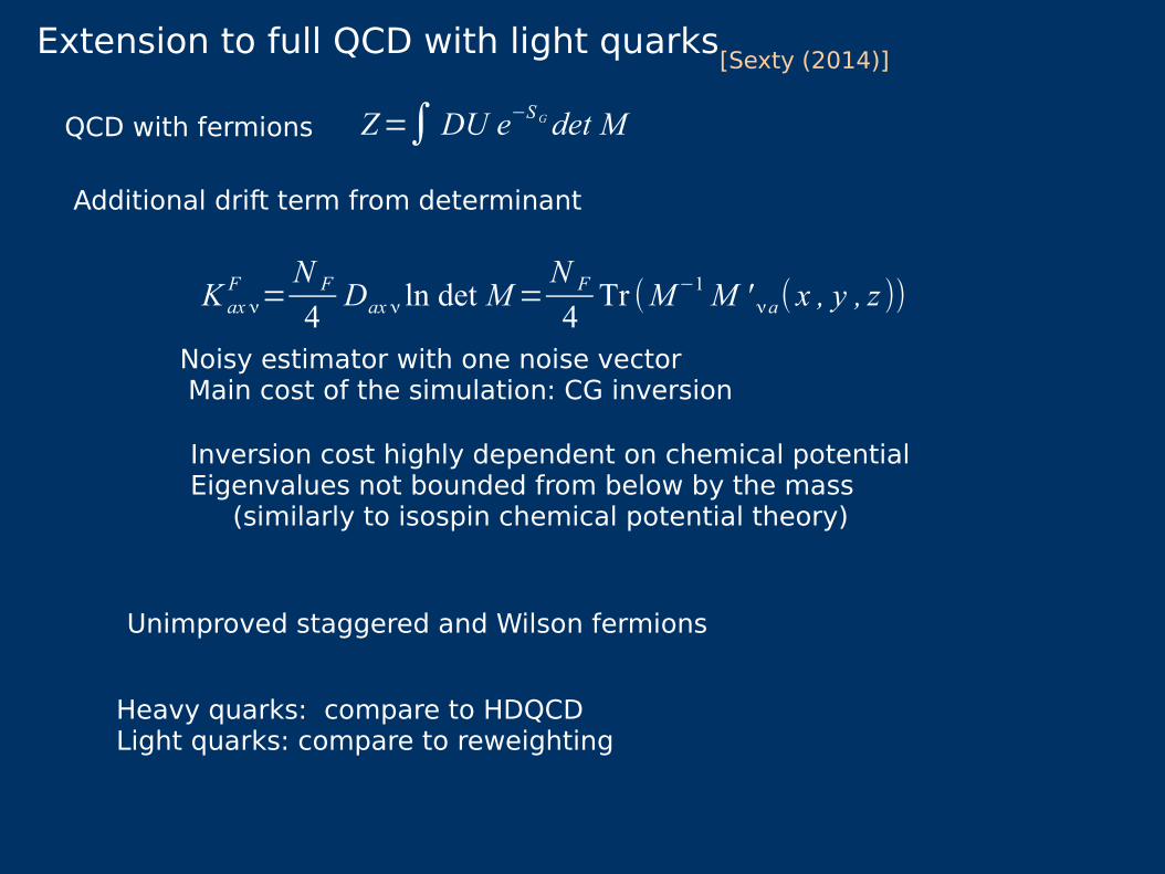
CLE and full QCD with light quarks [Sexty (2014)]

Non-holomorphic action poles in the fermionic drift

Is it a problem for full QCD?

So far, it isnt:Comparison with reweightingStudy of the spectrumHopping parameter expansion

Physically reasonable results

Comparison with reweighting for full QCD

[Fodor, Katz, Sexty (in prep.)]

R=Det M (μ=0)

Reweighting from ensemble at

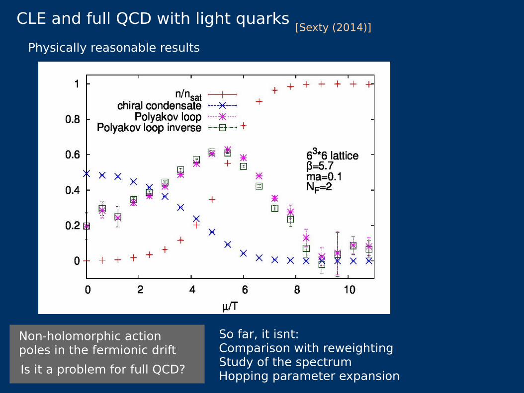
Sign problem

Sign problem gets hard around μ/T≈1−1.5

⟨exp(2 iϕ)⟩= ⟨det M (μ)

det M (−μ) ⟩

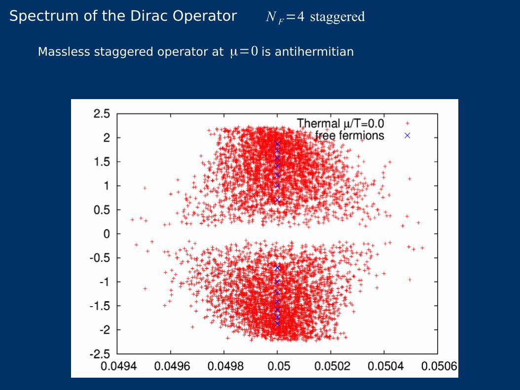
Spectrum of the Dirac Operator N F=4 staggered

Massless staggered operator at is antihermitianμ=0

Spectrum of the Dirac Operator N F=4 staggered

Conclusions

Recent progress for CLE simulations Better theoretical understanding (poles?) Gauge cooling Kappa expansion Two novel implementations with CLE: kappa and kappa_s Calculations at very high orders are feasible Convergence checked explicitly Shows that poles give no problem in QCD

Phase diagram of HDQCD mapped out

First results for full QCD with light quarks No sign or overlap problem CLE works all the way into saturation region Comparison with reweighting for small chem. pot. Low temperatures are more demanding

Direct simulations of QCD at nonzero density using complexified fields Complex Langevin Equations

Backup slides

Conclusion

QCD = HQCD for quark mass > 4/a

(For large mass) HQCD is qualitatively similar to QCD

Phasequenched vs full

in phasequenched P=P−1

in full theory, inv. Polyakov loop rises first

Reweighting form PQ theory better than Reweighting from ? μ=0

Z=∫dU e−Sg|det M|

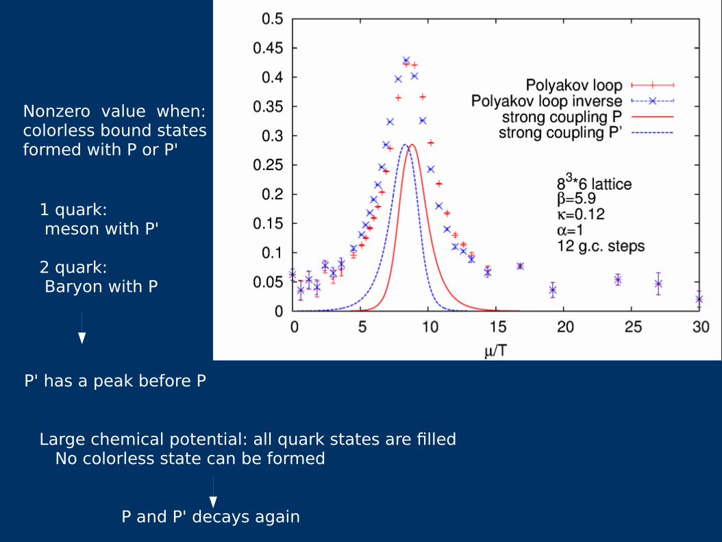
Nonzero value when:colorless bound states formed with P or P'

1 quark: meson with P'

2 quark: Baryon with P

P' has a peak before P

Large chemical potential: all quark states are filled No colorless state can be formed

P and P' decays again

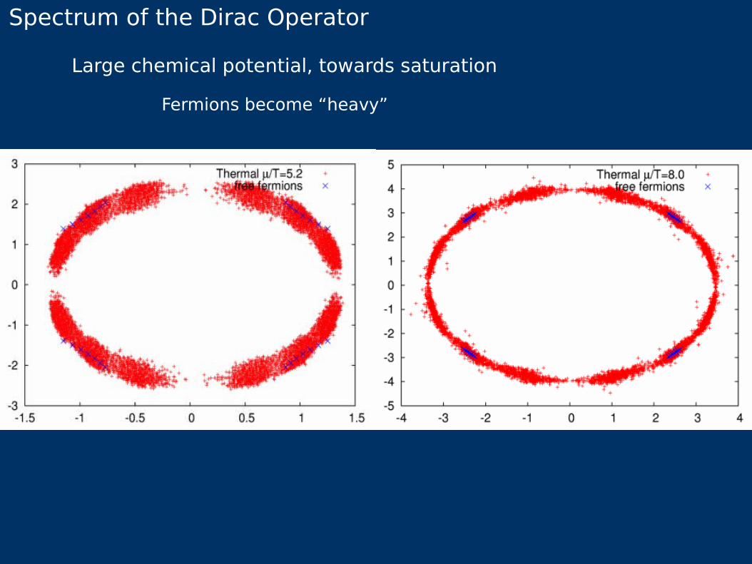
Spectrum of the Dirac Operator

Large chemical potential, towards saturation

Fermions become “heavy”