diversification versus concentration: the winner is
TRANSCRIPT

Diversification versus Concentration . . . and the Winner is?
Danny Yeung*
Paolo Pellizzari**
Ron Bird†***
Sazali Abidin****
The Paul Woolley Centre for the Study of Capital Market Dysfunctionality, UTS
Working Paper Series 18
Abstract: Diversification has its obvious benefits but its pursuit can involve a
trade-off between risk-controls and returns. We investigate this trade-off by
examining the relative performance of diversified versus concentrated portfolios
both formed on the basis of the same stock preferences. Using US equity mutual
funds as our data base, we establish that the concentrated portfolios achieve the
better performance. This highlights the potential for investors to diversify across
concentrated funds rather than have the funds do the diversification themselves. It
also highlights that the stocks selection skills of the managers may be lost by their
portfolio construction endeavours.
* Paul Woolley Centre, University of Technology Sydney
* *University of Venice
*** Paul Woolley Centre, University of Technology Sydney and School of
Management, Waikato University
**** School of Management, Waikato University
† Corresponding author:
Paul Woolley Centre for the Study of Capital Market Dysfunctionality
University of Technology Sydney
Quay Street, Haymarket NSW Australia 2007
Phone: +612 95147716
Fax: +612 95147722
Email: [email protected]

2
In the blue corner we have the great diversifiers ably led by Harry
Markowitz, Bill Sharpe and other protagonists from the Modern Portfolio Theory
(MPT) school. In the red corner we have the celebrated concentrators including
John Maynard Keynes, Warren Buffet and a score of other like-minded
practitioners. The concentrators fell out of favour among the investment
community over 50 years ago when the MPT people showed us the advantages of
diversifying our asset holdings. They demonstrated that by so doing we reduced
the risk of holding these assets and if we choose not to diversify that we would be
paying too much for them. Somewhat persuaded by these arguments, but also
driven by their clients, the professional fund managers moved to holding widely-
diversified, risk-controlled portfolios (i.e. from being concentrators to diversifiers).
It was only a decade or so after this transition began that many of the great
diversifiers began telling the professionals that they were not doing a good job for
their clients. That as a group they were only average and that they actually
detracted from their clients’ wealth once account was taken of fees. Still,
diversification remained the main game into the new millennium with little or no
connection being made between the apparent lack of skills displayed by the
professional managers and the mantra of diversification. With the bursting of the
dot.com boom in early 2000s, we saw an increased interest in more concentrated
portfolios under the guise of absolute return funds driven by investors seeking a
continuation of the high returns that they had been enjoying for the previos two
decades. Along with this shift in demand we saw a re-emergence of the debate as
to the relative benefits associated with running diversified versus concentrated
portfolios.
It is this debate that we take up in this paper where we use US equity
mutual fund data to examine how the managers would have performed if they
pursued more concentrated portfolios. We exclude funds that are already
concentrated and for the remainder identify the manager’s preferred stocks. We
then form concentrated portfolios based on these preferred stocks where the size of
these portfolios range from 5 to 30 stocks. As would be expected the more
concentrated portfolios, the higher its absolute risk (as measured by the standard
deviation of its returns) and also its risk relative to the benchmark (as measured by
its tracking error). More importantly, we find that the concentrated portfolios
outperform both the actual performance of the fund and its benchmark. Risk-
adjusted performance also tends to be higher for the more concentrated portfolios
as compared to the actual portfolios and the benchmark.
These findings are basically good news for the professional managers who
have long been criticised for their performance. The evidence suggests that they
are actually good at what they spend most of their time doing, selecting stocks.
The problem is that they are stripped of this edge due to having to depart from
their stock preferences in the interests of diversification and risk-control. This is

3
not to downplay the importance for investors of running a diversified portfolio
across all of its investments but it does question the current practice of requiring a
high degree of diversification of individual managers.
The remainder of the paper is structured as follows. In section 1, we outline
the nature of the issue that we are addressing drawing where possible from the
available literature. Section 2 is devoted to outlining our data and the methods that
we employ in our analysis. We present and discuss our findings in Section 3.
Section 4, provides us with the opportunity to summarise.
Section 1: Background
The major advance of our understanding of risk came with the work by
Harry Markowitz (1952) on portfolio theory. This work completely changed our
view on portfolio construction by demonstrating that we should no longer assess
risk at the level of individual securities but rather in terms of the contribution that
each security makes to the total portfolio. The investment process involves
assessing the potential of the securities in our universe to generate returns and
then combining these securities in a portfolio to generate acceptable risk-return
outcomes. The work of Markowitz switched our attention back to the portfolio
construction phase where risk plays a much more equal role to returns in
determining where the funds are invested. In particular, we learned from MPT the
need to diversify our portfolios and by so doing achieve risk-reduction. By not
diversifying we would be taking on risks that are not compensated by the market
and so effectively paying too much for our securities.
The need to embrace diversification was not only accepted by the funds
management community because they were convinced that it was a good idea but
also because it rapidly came to be accepted as prudent practice by the regulators
and their clients. For example, it is embedded in the “prudent man” principles that
govern fiduciaries1. As a consequence, we find that almost all product description
statements or investment mandates that govern how funds are invested will have
many explicit and implicit statements that drive the manager towards holding
diversified portfolios. Hence over the second half of the 20th century we moved to a
world governed by the diversifiers.
The question that we pose here is whether the benefits associated with
diversification come at a cost in terms of foregone returns? The answer is
potentially yes as there may be a conflict between investing in the stocks that are
1 The Employee Retirement Income Security Act (“ERISA”) was enacted into law in the US in
1974. ERISA enforces the administration of retirement and benefit plans. ERISA has a Diversification Rule
– A fiduciary must diversify investments in order to minimize risk of loss unless it would be considered
prudent to not diversify investments. 29 U.S.C. §1104 (a)(1)(C).
4
cheap and investing in stocks that bring the greatest diversification advantages to
the portfolio. It is important to note here that there can be no conflict if markets are
efficient as then there are no market mispricings to exploit and so portfolio
construction is the only game in town. Of course many would disagree about the
efficiency of markets or otherwise why would so many resources be devoted to
identifying mispriced stocks. Perhaps the best expression that we have of the
dangers of diversification comes from one of the greatest intuitive investment
thinkers of all time, John Maynard Keynes, who wrote to a friend in 1934:
“As times goes on, I get more and more convinced that the right
method of investment is to put large sums into enterprises
which one thinks one knows something about and in the
management of which one thoroughly believes. It is a mistake to
think one limit’s one’s risk by spreading too much between
enterprises about which one knows little and has no reason for
special confidence.”
The insights provided by Keynes have not been lost on many of the greatest
investors of our time, such as Warren Buffet and George Soros, who are firmly in
the camp of the concentrators. Of course, the one feature that is common to all of
the well regarded concentrators is their ability to choose stocks. Without this
special ability, a manager would be well-advised to limit the bets that they take or
probably better, offer index funds. The reality is that the majority of funds are
invested with active managers which either suggests that there is a surfeit of
managers with the ability to outperform and/or only a weak relationship between
a manager’s stock selection ability and his willingness to take bets. On this latter
point, Bird et al. (2011) have demonstrated that given investors tend to chase
outperformance, even managers with negative ability have strong incentives to
take sizable bets in the hope of fluking some significant outperformance. Therefore
we cannot conclude that the fact that we have many managers willing to take
active bets as being indicative that we have a large number of managers with the
ability to identify mispriced stocks.
Perhaps to obtain better insights into the true ability of active managers we
should explore the available literature of which there is ample. The studies of the
performance of active funds are numerous dating back to the mid-60s with the
general finding being that as a group they underperform their benchmark once
account is taken of their management fees and the other incremental costs
associated with employing active managers (Jones and Wermers, 2011). Of course,
the fact that active management as a whole fails to outperform does not preclude
that many managers will outperform their benchmark over any particular
measurement period2. However given that most managers are appointed on the 2 Jones and Wermers, (2011) recommend the taking account of the following four factors when trying to
identify superior managers: (i) past performance, (ii) macroeconomic forecasting, (iii) fund/manager
characteristics, and (iv) analysis of fund holdings.

5
basis of their past performance, this will only translate into value-adding future
outperformance for investors if it proves that there is a high level of persistence in
manager performance (Gohal and Wahal, 2008). Again the empirical evidence
suggests that there is little persistence in fund performance which adds to the
argument that investors would be well advised to delegate the majority of their
funds to low costs passive management (Busse et al., 2010).
The implications commonly drawn from these findings is that (i) managers
as a group underperform on an after-fees basis and (ii) markets are efficient given
that highly-paid professions managers are unable to identify mispriced stocks.
These issues are no where near as clear-cut as one might think with one possible
interpretation of the empirical findings being that securities are often mispriced
and funds managers are quite good at identifying these mispricing but that the
profit-making potential of this ability is either diluted or destroyed by a number of
factors including the risk controls introduced at the portfolio construction stage.
The other particularly relevant literature comes from the recent work on the
relationship portfolio concentration and fund performance. The common finding
of most of this research is that on average the more concentrated portfolios
outperform their benchmarks on an after-fees basis (Kacpercyzyk et al., 2005;
Brands et al., 2005; Cremers and Petajisto, 2009). Bird et al. (2011) have shown that
it is optimal for the more skilled managers to run the more concentrated portfolios
suggesting that there may be self-selection with the better managers running the
more concentrated portfolios and achieving the better performance. Cohen et al.
(2010) show that the absolute best idea of a fund managers (i.e. the stock that they
like most) systematically outperforms the portfolios actually run by the manager.
Overall, the results from prior research raise the possibility that if fund managers
invested in concentrated portfolios based on their best ideas, they would
significantly improve their performance over that realised from investing in more
diversified portfolios. The remainder of this paper is aimed at providing more
clarification on the important contest between the diversifiers and the
concentrators. The determination of the winner of this contest will have several
important implications. The first being as to how investors should optimally use
fund managers when structuring their investments. An option being that they
allow the managers to run concentrated funds and then to combine the funds in a
way to realise the diversification benefits. Our findings will also provide insights
into the contributions made by fund managers. The possibility that the average
manager has above average stock selection skills brings into question the
conclusion drawn from the fund performance literature that as a group they offer
little to clients who would be well advised to invest via index funds. A third
important implication of our findings relates to the efficiency of markets. If
managers display the ability to outperform running concentrated portfolios, then
this suggests that they can consistently identify mispriced stocks. Finally, if we do

6
find evidence to suggest that managers are good at stocks selection, then the
question is why does this not translates into better overall investment
performance. The suggestion is that the benefits from their superior stock selection
skills are lost in the portfolio construction stage of the process as a result of the
inclusion of many stocks in the portfolio for risk-control purposes rather than
because they are considered mispriced.
Section 2: Data and Methodology
The Data
Our data set extends from 1999 to 2009 with the majority of the data being
collected on a quarterly basis. All but the holdings data for the funds is obtained
from CRSP Survivor-Bias-Free US Mutual Fund Database. Fund Holdings data is
obtained from Thomson Reuters S12 Mutual Fund Holdings.3 Data for the indices
used are obtained from Russell Company and Standard and Poors. Finally we
obtained our stocks returns data from Compustat. We make use of the
CRSP/Compustat Merged Database (CCM) to link the stock data to funds
information to perform our analysis. The data for the four factors used in the
Carhart model were obtained from Kenneth French’s website.
Sample and Data Selection
The fund selection process began by collecting quarterly data for actively
managed funds from the universe of CRSP Survivor-Bias-Free US Mutual Fund
Database.4 Because we want to deal with diversified portfolios, we deleted from
any funds with an average holding of less than 40 stocks5. Some sample statistics
for our final sample of 4,723 actively managed are reported in Table 1. The average
fund size is $306m with an average fund holding of more than 150 stocks. Our
sample contains a lot of embryonic funds with very low funds under management
and relatively low stock holdings. When growth and value managers are evaluated
separately, the value managers are slightly larger both in terms of funds under
management and also stock holdings. Finally, Table 1 reports that there are 1659
institutional funds and 3069 retail funds in the sample. While the average retail
fund tends to have larger funds under management, the median institutional fund
has slightly higher fund under management than the median retail fund. The
finding may reflect that institutional investors are more aware that there is an
optimal fund size above which fund returns will decrease.
3 Given that CRSP fund holdings data was only available from 2003, the use of Thomson Reuters S12 Fund
holdings data enables us to significantly expand the sample period. 4 Consistent with other studies in the mutual fund area, we use the funds’ strategic objective provided by
CRSP to filter our sample. Since CRSP provide several sets of strategic objectives (namely Strategic Insights
and Lipper Investment Objectives) and neither set of strategic objectives data covers the entire sample period,
we use a combination of Strategic Insights and Lipper Investment Objectives to filter our final sample. We
selected funds with the following Lipper Investment objectives: G, GI, LSE, MC, MR and SG. Funds from
the Strategic Insights objective codes, we selected AGG, GRI, GRP, ING, SCG and GMC. 5 The literature suggests that the majority of the benefits of diversification are obtained by the time that the
portfolio size has reached 40 securities (Tang, 2004)

Table 1 Summary Statistics
This table shows the summary statistics of the sample of mutual funds in the period 1999 to 2009. Fund size represents the total net asset of the company. We report the
characteristics of the fund size fund size and the average number of stocks held by the funds. The table contains statistics for the full sample as well as subsample of
funds. We classify managers into Growth, Value and Style Neutral based on the designated benchmark index. For example, the sample of Value managers
contains all the funds that have a value index (i.e. S&P400 Value, S&P500 Value, S&P600 Value, Russell 1000 Value, Russell 2000 Value and Russell Mid Value) as
its designated benchmark. From the sample of active funds, we were able to classify the Institutional funds in our sample through the use of the institutional fund
identifier (inst_fund) from CRSP. The remainder of the sample of funds are classified as Retail mutual funds.
Full Sample Small Large Growth Value Institutional Retail
Fund Size ($’M)
Number Of
Stocks
Fund Size ($’M)
Number Of
Stocks
Fund Size ($’M)
Number Of
Stocks
Fund Size ($’M)
Number Of
Stocks
Fund Size ($’M)
Number Of
Stocks
Fund Size ($’M)
Number Of
Stocks
Fund Size ($’M)
Number Of
Stocks
Mean 306 153 7 128 867 184 302 95 381 110 214 184 355 138
Median 50 87 6 86 293 93 43 80 50 79 54 93 46 84
Standard Deviation
1614 257 4
148 2709 329 1241 78 1490 119 913 314 1747 224
Min 1 41 1 41 93 41 1 41 1 41 5 41 1 41
Max 60890 3561 16 1891 60890 3561 24288 933 25101 1653 30647 3501 59756 3561
Number Of Funds
4723 1574 1575 1491 835 1654 3069

The Methodology
Benchmark Assignment and Active Position
An essential part of our analysis is the assignment of a benchmark to each fund in
our sample. We do so using a measure that we refer to as the fund’s active position which
is half the aggregate of the absolute differences between the fund’s holdings and the
index weight for each stock. Consistent with Cremers and Petajisto (2009), we estimate
the level of active management by comparing the holdings of a mutual fund with the
stocks weightings of 18 different indices. We collected index compositions data for a total
of 18 equity market indexes of which nine belonged to the Russell family (namely the
Russell 1000, Russell 2000, and Russell Midcap indexes, plus the value and growth
components of each) and the other nine being sourced from Standard and Poors (the
S&P400, S&P500 and S&P600 indexes, plus the value and growth components of each)6.
We determine each quarter the index that most closely tracks each fund’s actual portfolio
(i.e. the index that gives it the smallest active position). As a consequence over the life of
each fund we have a benchmark index assigned each quarter. We then allocate to each
fund as its benchmark, that index that was chosen in the greatest number of quarters. In
this way, we are able to maintain the principle of choosing the index that is closest to the
actual holdings while being able to maintain a single benchmark over the life of the fund.
Portfolio Weights and Returns
Concentrated Portfolio Construction
Each quarter, we measure the difference between each fund’s portfolio holdings
and the holdings of the assigned bench mark index (the “bet size” for each stock)7. The
differences can be thought of as a measure of the degree of confidence that the manager
has for that stock to yield superior returns. We sort these bets by size from the largest. We
then build each quarter concentrated portfolios varying in size from five stocks (Top 5) to
30 stocks (Top 30) where the stocks included are based upon these rankings (i.e. the top
five stocks in the Top 5 portfolio, and so on).
Portfolio Weights and Returns
We use two set of portfolio weights in our analysis, equal weighting and
“conviction” weighting. Equal weighting assumes that managers will invest at the
beginning of each quarter an equal proportion of funds in each stock within the portfolio.
For example, a manager will invest 10% of funds in each stock within the Top 10
concentrated portfolio. In the case of equal weighting, the portfolio returns each quarter
will be the average quarterly returns of the stocks within the portfolio.
We also implement a second set of weights, “conviction weights”, for the concentrated
portfolio. We believe that conviction weights are informative because it takes into
6 We wish to thank Russells and Standard and Poor for providing this data
7 We also repeated the analysis using the S&P500 as the index for all funds. The basic results were unchanged
to those reported in this paper.

9
account both the index and the strengths of the manager’s opinion for each stock. The
conviction weight is calculated as follows:
( )
(
)where
Indexholdingit is the index weight assigned to stock i in quarter t
SumofIndexholdingst represents the aggregate of the index weights for each stock
included in the portfolio in quarter,t
BetSizeit represents the difference between the fund’s actual holdings of stock i in
quarter t and the index weight for that stock and the holdings in the benchmark
index
SumOfBetst is the sum the BetSizeit foe the stocks included in the portfolio
The quarterly returns of the concentrated portfolios are simply the sum of the weighted
average of the quarterly returns of all the stocks in the portfolio where the weights are
determined by the conviction weights.
Portfolio Performance and Excess Returns
The quarterly returns for the various portfolios are calculated on the presumption
that an equal amount is invested in each fund for which we have a portfolio for that
quarter. For example, if we have portfolio for a 1,000 funds for a particular quarter, then
we assume an investment of 0.1% in that fund for that quarter. Therefore, the return for
the portfolio for the quarter is the average of the quarterly returns for each of the funds
included that quarter. In this way, we calculate the returns for the Top 5 through to Top
30 portfolios over the 44 quarters in our sample. Using these returns we can then
calculate the annualised returns for each portfolio, its standard deviation and its Sharpe
ratio8.
As well as calculating the absolute return for each concentrated portfolio each
quarter, we also calculate its excess return. These excess returns are calculated relative to
the following three sets of returns: the fund’s actual returns, the returns on its own
assigned index and the returns on the S&P500 index. Using the same procedure as
previously, we use these quarterly excess returns to calculate the annualised excess
return for each concentrated, Top 5 through to Top 30, its tracking error (which is the
standard deviation of the quarterly excess returns) and its information ratio (which is the
annualised excess return divided by its tracking error). Finally we used 4-factors model
developed by Carhart (1997) to determine risk adjusted alphas for the concentrated
portfolios and to examine their risk exposures.
8 See Sharpe (1966)
10
Section 3: Findings
Absolute Returns
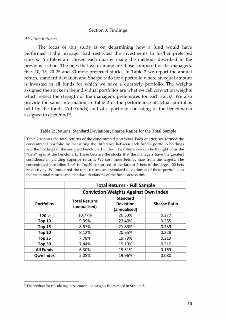
The focus of this study is on determining how a fund would have
performed if the manager had restricted the investments to his/her preferred
stock’s. Portfolios are chosen each quarter using the methods described in the
previous section. The ones that we examine are those composed of the managers,
five, 10, 15, 20 25 and 30 most preferred stocks. In Table 2 we report the annual
return, standard deviation and Sharpe ratio for a portfolio where an equal amount
is invested in all funds for which we have a quarterly portfolio. The weights
assigned the stocks in the individual portfolios are what we call conviction weights
which reflect the strength of the manager’s preferences for each stock9. We also
provide the same information in Table 2 of the performance of actual portfolios
held by the funds (All Funds) and of a portfolio consisting of the benchmarks
assigned to each fund10.
Table 2: Returns, Standard Deviations, Sharpe Ratios for the Total Sample
Table 2 reports the total returns of the concentrated portfolios. Each quarter, we formed the
concentrated portfolio by measuring the difference between each fund’s portfolio holdings
and the holdings of the assigned bench mark index. The differences can be thought of as the
“Bets” against the benchmark. These bets are the stocks that the managers have the greatest
confidence in yielding superior returns. We sort these bets by size from the largest. The
concentrated portfolios Top5 to Top30 comprised of the largest 5 bets to the largest 30 bets
respectively. We measured the total returns and standard deviation as of these portfolios as
the mean total returns and standard deviations of the funds across time.
Total Returns - Full Sample Conviction Weights Against Own Index
Portfolios Total Returns (annualised)
Standard Deviation
(annualised) Sharpe Ratio
Top 5 10.77% 26.33% 0.277
Top 10 9.39% 23.40% 0.255
Top 15 8.67% 21.83% 0.239
Top 20 8.12% 20.65% 0.228
Top 25 7.78% 19.79% 0.219
Top 30 7.44% 19.13% 0.210
All Funds 6.30% 19.51% 0.169
Own Index 5.05% 19.96% 0.080
9 The method for calculating these conviction weights is described in Section 2.

11
The major insight provided by Table 2 is that the concentrated portfolios as
a group outperform both the actual (diversified) portfolios implemented by the
funds and also their benchmarks. Further, the more concentrated the portfolio, the
better the performance as we see a progressive decrease in realised returns as the
concentrated portfolios are expanded from five stocks to 30 stocks. This provides
strong evidence that the portfolio construction phase of the investment process is
resulting in reduced returns. As one would expect, the concentrated portfolios
have higher total risk as measured by the standard deviation of the returns.
However, these progressively decrease as the number of stocks in the concentrated
portfolios increase. Indeed by the time the portfolio holdings increase to 25 to 30
stocks, the standard deviation for the concentrated portfolios are equivalent to
those for the diversified portfolios which is consistent with previous evidence on
the number of stocks required to include in a portfolio to gain the majority of the
advantages’ of diversification. Given our findings on returns and standard
deviations, it is not surprising that the concentrated portfolios have a higher
Sharpe ratio to those of the actual funds and also the funds’ indices. Again, the
Sharpe ratio of the concentrated portfolios consistently declines as we expand their
portfolio size. All of our findings suggest that we have been effective in using the
actual portfolios of the funds to determine the relative preferences of the managers
for the stocks that they include in their portfolio. The conclusion that we would
draw from the information contained in table 2 is the managers of mutual funds as
a group have good stock selection skills but that these are diluted by the portfolio
construction process.
Excess Returns
We next evaluate the performance of the same portfolios where we
measured the return of the concentrated portfolios relative to both the actual
portfolios that they held (i.e. Own Funds) and their own benchmark (i.e. Own
Index)11. The results reported in Table 3 present a similar picture to what we saw in
Table 2 with both the outperformance and the risk as measured by the tracking
error reducing as the concentrated portfolio is diluted. It has to be remembered
that these results represent the performance across several thousand mutual funds
and so report the performance of the average fund. Again they confirm the ability
of the average manager to identify mispriced stocks with the information ratio
indicating that they can add value on a risk-adjusted basis.
11
We obtained similar results when we evaluated the excess returns relative to the S&P500.

12
Table 3: Excess Return, Tracking Error and Information Ratio for Total Sample
Table 3 reports the excess returns of the concentrated portfolios. Each quarter, we formed the concentrated
portfolio by measuring the difference between each fund’s portfolio holdings and the holdings of the assigned
bench mark index. The differences can be thought of as the “Bets” against the benchmark. These bets are the
stocks that the managers have the greatest confidence in yielding superior returns. We sort these bets by size
from the largest. The concentrated portfolios Top5 to Top30 comprised of the largest 5 bets to the largest 30 bets
respectively. We reported the excess returns of the portfolios in comparison to the fund’s actual performance
and the performance of the benchmark index. Tracking error is measured as the standard deviation of the excess
returns. Information Ratio is calculated as the. We reported the excess returns, tracking error and information
ratio as of these portfolios as the mean excess returns, tracking error and information ratio of the funds across
time.
Conviction Weighted Portfolios
Concentrated Portfolios
Relative to 0wn Fund Relative to Own Index
Excess Return (% pa)
Tracking Error (%pa)
Information ratio
Excess Return (% pa)
Tracking Error (%pa)
Information ratio
Top 5 3.75 16.49 0.23 5.26 17.68 0.30
Top 10 2.41 12.94 0.19 3.90 14.06 0.28
Top 15 1.69 11.00 0.15 3.16 12.12 0.26
Top 20 1.17 9.62 0.12 2.67 10.68 0.25
Top 25 0.83 8.69 0.10 2.30 9.69 0.24
Top 30 0.52 8.04 0.07 1.97 9.00 0.22
Carhart 4-factor Model
The final piece of analysis using our total sample is to subject our
concentrated portfolios to the Carhart four-factor model. The dependent variable in
our variable is the average quarterly return on our concentrated portfolios derived
using each fund’s own benchmark, less the risk-free rate. The risk-adjusted
performance as indicated by the constant (alpha) as reported in Table 4 suggests
that the outperformance of the concentrated portfolios ranged from slightly in
excess of 5.1% pa for the Top 5 portfolio to about 2.1 % pa for the Top 30 portfolio12.
The market beta for the portfolios commences above one for the most concentrated
portfolio and quickly falls to be insignificantly different to one as the concentration
is diluted. The strongest tilt across the funds is towards strong momentum stocks
with much weaker tilts towards small cap and growth stocks. Based on these
findings, again it appears that managers have stock selection skills which they do
not exploit when building diversified portfolios.
Table 4: Four Factor Model Applied to Total Sample
12
We conduct time series analysis based upon 43 quarterly observations. The sample size is a constraint on
being able to identify significant relationships.

13
We applied the Carhart four-factor model to the quarterly returns of the concentrated portfolio to control for risks.
The Carhart four-factor model coefficients are reported in the table. Rm-Rf is the coefficient associated with the
market premium (market returns less the risk free returns), SMB is the size premium (small stocks minus big
stocks), HML is the book-to-market premium (high minus low book-to-market stocks) and momentum is the 11
month less one month momentum factor. We reported the coefficients and the p-values in the table below.
Conc. Port.
Four Factor Model : Excess Returns based on Weighting against Own Index
Alpha P-Value Rm-Rf P-Value SMB P-Value HML P-Value Momentum P-Value
Top 5 1.246 0.307 1.249 0.088 0.143 0.542 -0.195 0.230 0.405 0.010
Top 10 0.955 0.321 1.168 0.143 0.121 0.515 -0.128 0.319 0.342 0.006
Top 15 0.790 0.339 1.118 0.228 0.111 0.488 -0.090 0.410 0.305 0.005
Top 20 0.680 0.350 1.077 0.371 0.099 0.480 -0.060 0.534 0.275 0.004
Top 25 0.599 0.363 1.044 0.573 0.092 0.468 -0.037 0.670 0.253 0.003
Top 30 0.528 0.386 1.015 0.830 0.088 0.452 -0.020 0.801 0.235 0.003
We plot in Figure 2 distribution of the excess annual returns for the Top 5
and Top 20 concentrated portfolios based on the excess returns over benchmark for
each fund included in our sample.13. As we have seen previously, both the average
and standard deviations of the excess returns decrease as we increase the size of
the concentrated portfolio. The values for the percentile cut-offs and the fact that
the mean excess return for the concentrated portfolio is much greater than its
median highlights are strong indicators that excess returns of the individual
concentrated funds are skewered towards the higher returns (i.e. to the right). This
is further confirmed by observing that average positive excess return of the funds
outperforming their benchmark is much greater than average negative return for
those funds that underperform. Therefore, if only 50% of the funds had a positive
excess return, the average returns over all managers would also be positive.
However, the information provided at the bottom of Figure 1 indicates that this
percentage of managers outperforming ranges from 55.65% for the Top 5 portfolio
to 53.09% for the Top 30 portfolio14. In summary, then average return of the
concentrated portfolios is positive because (i) the majority of these funds
outperform and (ii) those that do outperform on average do better in absolute
terms than those that underperform.
The other issue that we would like to address when discussing our whole
sample is the timing of the outperformance of the concentrated portfolios. When
we analyse their performance over the 11 years covered by our sample, we find
that they outperformed for five of these years and underperformed for six. As
must be the case given our overall finding of outperformance, their added value in
13
The excess returns reported are measured relative to the fund’s benchmark. 14
It would be wrong to use 50% as the point of comparison for the percentage of actual manager’s
outperforming, The reason be in that on average only 43% of the stocks in the common indices outperform in
a particular year which means that 43% of the stocks held included in an index fund would outperform. This
makes an outperformance of between 53% and 55+% of our funds look quite impressive.

14
the good years exceeds the detracted value in the bad years. It may not come as a
surprise to find that the good years for the concentrated portfolios are confined
largely to periods when the market was performing well. This finding is totally
consistent with the overall tilt in the concentrated portfolios towards relative small
positive momentum stocks which are the types of stocks that tend to during
periods of strong market sentiment. This suggests that investors would be best
placed favouring concentrated funds when market sentiment is high but switch to
more diversified funds when overall gloom descends on markets.
Investment Styles
Of interest is whether our findings over the total sample hold for important
sub-sets of the sample. In this case we have repeated much of the analysis where
the total sample is divided on the basis into style neutral, value and growth
funds15. In Table 5 we report the annualised return, standard deviation and Sharpe
measures for the concentrated portfolios for each style of fund. In addition we
provide for each style both the actual returns achieved plus the returns achieved
by their benchmarks (with also standards deviations and Sharpe measures for
each). All three styles display the same finding as previously with the returns,
standard deviations and Sharpe measures reducing as the concentrated portfolios
are diluted. By far the greatest returns are realised by the concentrated portfolios
operated by the growth managers with their “Top 5” portfolios outperforming
their actual performance by almost 8% per annum. However, this very good
performance is somewhat facilitated by the fact that growth indices are populated
by stocks with high valuation multiples (i.e. “expensive” stocks) making it easier
for the growth managers to identify mispriced stocks in their universe. Still it
remains impressive that the average growth manager can maintain a relatively
good information ratio even for their Top 30 portfolio. In the case of the value and
market neutral funds, they can both produce a reasonable performance for their
more concentrated portfolios which dissipates at a slightly faster rate than it does
for the growth funds16. We have reported previously that the actual returns are
after transaction costs while the other returns are all before transaction costs. Once
these are added back to the actual returns it proves that all of the concentrated
portfolios of the growth managers handsomely outperform their actual returns
9adjsuted for transaction costs and the returns on their benchmark. The story for
the style neutral and value managers is not quite as good with their actual
performance (adjusted for transaction costs) equating with that of their “Top 20”
concentrated portfolio with their more concentrated portfolios still outperforming.
15
This division is done on the basis of the fund’s benchmark. 16
We also conducted identical analysis where all performance was evaluated relative to a common index
(S&P500). In this case, the performance of the concentrated for the value funds was almost as impressive as
that of the growth managers. Consistent with Bird et al (2011), this confirms that the growth managers have
an advantage in implementing their portfolios but that the value style brings higher returns than does the
growth style (consistent with there being a positive value premium)

Distribution of Excess Returns Concentrated Portfolios
Top5 Top10 Top15 Top20 Top25 Top30
Mean 5.82% 4.24% 3.52% 2.88% 2.46% 2.09%
Std Deviation 15.73% 12.02% 10.59% 9.43% 8.53% 7.90%
10th Percentile -15.21% -12.84% -11.03% -10.17% -9.50% -9.35%
25th Percentile -6.73% -5.40% -4.85% -4.62% -4.22% -4.04%
Medians 1.47% 1.32% 1.05% 0.74% 0.73% 0.49%
75th Percentile 11.68% 8.93% 7.93% 6.73% 6.35% 5.87%
90th Percentile 30.49% 22.91% 20.25% 16.83% 15.82% 13.74%
Positive Excess Returns 55.65% 55.01% 54.99% 54.19% 53.89% 53.09%
Mean of Positive Excess Returns Fund 21.49% 16.28% 13.86% 12.25% 11.07% 10.30%
Mean of Negative Excess Returns Fund -11.63% -9.18% -8.15% -7.44% -6.95% -6.64%
Figure 1: Distribution of Excess Returns for Total Sample

Table 5 Returns, Standard Deviations and Sharpe Ratios for Different Investment Styles
Table 5 reports the returns of the concentrated portfolios for managers of different investment
styles. We classify managers into Growth, Value and Style Neutral based on the designated
benchmark index. For example, the sample of Value managers contains all the funds that have a
value index (i.e. S&P400 Value, S&P500 Value, S&P600 Value, Russell 1000 Value, Russell 2000
Value and Russell Mid Value) as its designated benchmark. We reported the returns, standard
deviations and Sharpe ratio as of these portfolios as the mean returns, standard deviations and
Sharpe ratio of the funds across time.
Conviction Weighted Portfolios: Market Neutral Funds
Concentrated Portfolios Conviction Weights Against Own Index
Total Returns Standard Deviation Sharpe Ratio
Top 5 8.33% 22.17% 0.22
Top 10 6.93% 19.51% 0.18
Top 15 6.18% 18.24% 0.15
Top 20 5.59% 17.29% 0.12
Top 25 5.34% 16.61% 0.11
Top 30 5.14% 16.12% 0.10
All Market Neutral Funds 4.40% 18.03% 0.08
Corresponding Index Ret 3.70% 18.27% 0.04
Conviction Weighted Portfolios: Value Funds
Concentrated Portfolios Conviction Weights Against Own Index
Total Returns Standard Deviation Sharpe Ratio
Top 5 11.20% 18.40% 0.43
Top 10 10.42% 16.83% 0.42
Top 15 9.48% 16.05% 0.38
Top 20 8.84% 15.46% 0.35
Top 25 8.41% 15.12% 0.33
Top 30 7.99% 14.82% 0.31
All Value Funds 8.11% 18.56% 0.27
Corresponding Index Ret 7.04% 19.23% 0.21
Conviction Weighted Portfolios: Growth Funds
Concentrated Portfolios Conviction Weights Against Own Index
Total Returns Standard Deviation Sharpe Ratio
Top 5 14.40% 31.30% 0.35
Top 10 12.86% 28.13% 0.33
Top 15 11.72% 26.14% 0.32
Top 20 10.81% 24.55% 0.30
Top 25 10.21% 23.34% 0.29
Top 30 9.69% 22.47% 0.28
All Growth Funds 6.64% 23.77% 0.15
Corresponding Index Ret 4.83% 22.84% 0.08
We next analysed the performance of the three styles using the Carhart
four-factor model and the results are reported in Table 6. Our findings show a clear
separation between the risk-adjusted performances of the concentrated portfolios
for each of the three investment styles: the growth funds with an annual risk-
adjusted return of 7.9%, the value with 4.9%, and the market neutral trailing with

17
2.8%. The market beta of the growth funds is consistently above one, with that of the
market neutral funds ranging both sides of one, and that for the value funds
typically being less than one. The preferred stocks by each style of management is
strongly tilted towards momentum stocks and each style of manager has a slight tilt
towards small cap stocks with this being greatest for the growth managers. Finally
true to label, the value funds have a value tilt, the growth funds have a growth tilt,
and the market neutral managers have no discernible tilt to either value or growth.
Table 6: Four Factor Model Applied to Different Investment Styles
Table 6 reports the Carhart four-factor model coefficients for the concentrated portfolios for managers of different
investment styles. We regress the quarterly returns of the concentrated portfolios against the Carhart four-factor
model. The Carhart four-factor model coefficients are reported in the table. Rm-Rf is the coefficient associated with
the market premium (market returns less the risk free returns), SMB is the size premium (small stocks minus big
stocks), HML is the book-to-market premium (high minus low book-to-market stocks) and momentum is the 11
month less one month momentum factor. We reported the coefficients and the p-values in the table below.
Conc. Port.
Four Factor Model : Excess Returns based on Weighting against Own Index for Market Neutral Funds
Alpha P-Value Rm-Rf P-Value SMB P-Value HML P-Value Momentum P-Value
Top 5 0.686 0.508 1.179 0.146 0.058 0.771 -0.118 0.391 0.368 0.006
Top 10 0.466 0.557 1.103 0.277 0.035 0.822 -0.057 0.588 0.304 0.004
Top 15 0.322 0.629 1.052 0.501 0.023 0.856 -0.021 0.809 0.268 0.002
Top 20 0.268 0.649 1.016 0.817 0.012 0.916 0.006 0.939 0.243 0.002
Top 25 0.218 0.683 0.983 0.789 0.010 0.923 0.027 0.699 0.224 0.002
Top 30 0.184 0.712 0.957 0.462 0.007 0.940 0.041 0.535 0.209 0.002
Conc. Port.
Four Factor Model : Excess Returns based on Weighting against Own Index For Value Funds
Alpha P-Value Rm-Rf P-Value SMB P-Value HML P-Value Momentum P-Value
Top 5 1.212 0.172 1.047 0.651 0.093 0.583 0.154 0.193 0.388 0.001
Top 10 0.950 0.170 0.983 0.834 0.075 0.572 0.210 0.025 0.327 0.000
Top 15 0.752 0.210 0.954 0.508 0.075 0.516 0.243 0.004 0.309 0.000
Top 20 0.610 0.261 0.921 0.218 0.076 0.467 0.263 0.001 0.284 0.000
Top 25 0.540 0.281 0.902 0.102 0.065 0.499 0.275 0.000 0.266 0.000
Top 30 0.445 0.342 0.883 0.038 0.065 0.474 0.285 0.000 0.250 0.000
Conc. Port.
Four Factor Model : Excess Returns based on Weighting against Own Index for Growth Funds
Alpha P-Value Rm-Rf P-Value SMB P-Value HML P-Value Momentum P-Value
Top 5 1.921 0.223 1.411 0.030 0.251 0.408 -0.465 0.030 0.428 0.032
Top 10 1.519 0.234 1.323 0.036 0.227 0.356 -0.382 0.028 0.370 0.023
Top 15 1.334 0.229 1.264 0.048 0.213 0.320 -0.340 0.025 0.324 0.022
Top 20 1.183 0.227 1.216 0.065 0.196 0.300 -0.300 0.024 0.285 0.022
Top 25 1.057 0.233 1.176 0.095 0.185 0.281 -0.271 0.025 0.259 0.022
Top 30 0.095 0.244 1.143 0.142 0.180 0.258 -0.246 0.027 0.239 0.022
Small versus Large Funds

18
There is evidence to suggest that large funds as a group underperform small
funds because as they grow they experience higher transaction costs (Chen et al.,
2005) and they become less aggressive in pursuing performance (Bird et al.,2011).
Therefore, comparing what managers might have achieved if they invested in their
preferred stocks provides a good opportunity to evaluate whether there is any
difference in the stock selection skills of those managing large and small funds. In
order to evaluate this we separated the sample into large (top third) and small
(bottom third) funds in terms of funds under management with the results of the
Carhart four-factor analysis being reported in Table 7. We find that the managers of
the larger funds have a slight edge over the managers of the small funds if they
restricted themselves to investing in concentrated portfolios composed of their most
favoured stocks: the Carhart alpha being 5.6% pa. for the large funds and 4.5% for
the small funds. There is little in the way of difference between the risks in the
portfolios of the large and small funds with all running large momentum tilts and
slight tilts towards growth and small cap stocks. The overall implication we draw
from our analysis is that the managers of the larger funds may have superior stock
selection skills so evidence of their underperformance suggests for some reason they
may be unwilling to fully exploit these superior skills
Table 7: Four factor Model Applied to Small and Large Funds
Table 7 reports the Carhart four-factor model coefficients for the concentrated portfolios for managers of different
sizes. We spilt the funds within our sample into terciles by their average size (as measured by the Tangible Net
Assets). We regress the quarterly returns of the concentrated portfolios against the Carhart four-factor model. The
Carhart four-factor model coefficients are reported in the table. Rm-Rf is the coefficient associated with the market
premium (market returns less the risk free returns), SMB is the size premium (small stocks minus big stocks), HML
is the book-to-market premium (high minus low book-to-market stocks) and momentum is the 11 month less one
month momentum factor. We reported the coefficients and the p-values in the table below.
Conc. Port.
Four Factor Model : Excess Returns based on Weighting against Own Index for Small Funds
Alpha P-Value Rm-Rf P-Value SMB P-Value HML P-Value Momentum P-Value
Top 5 1.111 0.356 1.235 0.103 0.134 0.564 -0.187 0.245 0.394 0.011
Top 10 0.833 0.368 1.152 0.166 0.110 0.536 -0.120 0.329 0.327 0.006
Top 15 0.689 0.390 1.107 0.258 0.103 0.505 -0.090 0.397 0.292 0.005
Top 20 0.593 0.400 1.068 0.411 0.089 0.513 -0.061 0.517 0.261 0.005
Top 25 0.522 0.413 1.037 0.643 0.082 0.506 -0.039 0.643 0.239 0.004
Top 30 0.452 0.444 1.009 0.895 0.078 0.496 -0.023 0.773 0.222 0.004
Conc. Port.
Four Factor Model : Excess Returns based on Weighting against Own Index For Large Funds
Alpha P-Value Rm-Rf P-Value SMB P-Value HML P-Value Momentum P-Value
Top 5 1.361 0.252 1.231 0.103 0.142 0.536 -0.183 0.247 0.403 0.009
Top 10 1.059 0.265 1.155 0.169 0.115 0.529 -0.115 0.363 0.342 0.005
Top 15 0.881 0.278 1.104 0.277 0.103 0.510 -0.077 0.474 0.305 0.004
Top 20 0.766 0.287 1.064 0.446 0.094 0.497 -0.047 0.621 0.277 0.003
Top 25 0.678 0.299 1.032 0.674 0.088 0.485 -0.024 0.777 0.256 0.003
Top 30 0.607 0.316 1.005 0.938 0.084 0.472 -0.008 0.922 0.240 0.003

19
Institutions versus Retail Funds
The final cut that we make in the data is between institutional and retail
funds. The little evidence available on the relative performance of these types of
managers is mixed. A very recent study by Del Guercio and Reuter (2011) found
that direct-sold retail funds outperformed institutional funds that in turn
outperformed broker-sold retail funds. In Tables 8 we report the results of applying
a Carhart 4-factor model to fund separated into retail and institutional. We find that
the level of outperformance of the concentrated portfolios of the institutional and
retail funds to be almost identical ranging from 5.1%pa for the most concentrated
portfolio to 2.1%pa for the least concentrated portfolio. Not only are the returns
realised almost identical but so are the risks and the portfolio characteristics. The
concentrated portfolios run by those managing retail funds and institutional funds
have the same strong tilt towards positive momentum stocks and relatively small
tilts towards growth stocks and small cap stocks that we have found previously.
Table 8: Four Factor Model Applied to Institutional and Retail Funds
Table 8 reports the Carhart four-factor model coefficients for the concentrated portfolios for managers of both the
Institutional and Retail funds. From the sample of active funds, we were able to classify the Institutional funds in
our sample through the use of the institutional fund identifier (inst_fund) from CRSP. The remainder of the
sample of funds are classified as Retail mutual funds. We reported the coefficients and the p-values in the table
below.
Conc. Port.
Four Factor Model : Excess Returns based on Weighting against Own Index for Institutional Funds
Alpha P-Value Rm-Rf P-Value SMB P-Value HML P-Value Momentum P-Value
Top 5 1.256 0.307 1.257 0.080 0.143 0.544 -0.202 0.219 0.404 0.011
Top 10 0.956 0.321 1.174 0.128 0.120 0.518 -0.131 0.306 0.339 0.007
Top 15 0.789 0.337 1.124 0.204 0.108 0.498 -0.092 0.398 0.302 0.005
Top 20 0.681 0.348 1.082 0.339 0.096 0.494 -0.062 0.517 0.271 0.004
Top 25 0.599 0.360 1.048 0.533 0.089 0.482 -0.039 0.653 0.249 0.004
Top 30 0.529 0.382 1.019 0.790 0.086 0.464 -0.022 0.785 0.231 0.004
Conc. Port.
Four Factor Model : Excess Returns based on Weighting against Own Index for Retail Funds
Alpha P-Value Rm-Rf P-Value SMB P-Value HML P-Value Momentum P-Value
Top 5 1.232 0.306 1.232 0.106 0.143 0.536 -0.181 0.258 0.406 0.009
Top 10 0.960 0.319 1.156 0.173 0.122 0.511 -0.119 0.352 0.346 0.006
Top 15 0.796 0.340 1.107 0.276 0.116 0.470 -0.085 0.441 0.310 0.004
Top 20 0.683 0.352 1.067 0.436 0.106 0.455 -0.055 0.574 0.281 0.003
Top 25 0.604 0.365 1.036 0.648 0.099 0.444 -0.033 0.709 0.259 0.003
Top 30 0.529 0.390 1.009 0.902 0.094 0.431 -0.017 0.839 0.241 0.003
Implementable Strategy
All the strategies that have been discussed to date have involved an equal
investment in each fund in existence at the beginning of each quarter. Although

20
analysis conducted on this basis is appropriate to address the relative benefits from
an investors’ perspective of funds running diversified versus concentrated
portfolios. However, it certainly does not reflect an implementable strategy
because investors will neither invest in hundreds of funds at the same time nor
will they rebalance their portfolio of funds on a quarterly basis. In this section, we
evaluate a strategy somewhat similar to that which could be pursued by a large
investor who puts together either a portfolio of diversified funds or a portfolio of
concentrated funds.
We initially divide the funds into nine groups based on their style (growth,
value and style-neutral) and market capitalisation (large cap, medium cap and
small cap). A diversified portfolio of concentrated funds (Top 5, Top 15, Top 25) is
created at the beginning of each quarter by a random choice of one (five) fund(s)
from each group with the return for that quarter being the average of the returns
realised by the nine concentrated funds. In this way the annual return for each of
the years in our sample is determined and so we can calculate the annualised
return for this single iteration of the strategy. We repeat this exercise 1,000 times
and measure the average return across these 1,000 simulations as being indicative
of the return that might be realise from a strategy where an investor follows a
strategy where the diversification is done by the investor who distributes his funds
across several concentrated funds. The above procedures are repeated where
rather than rebalancing the portfolios of managers quarterly, the rebalancing takes
place at three years intervals.
In a similar way we build portfolios of diversified funds following several
different strategies. The first of such strategies is where each quarter (each three
years) we just randomly choose a single fund from available at the time. We then
calculate the rate of return for each period using the actual returns realised by the
chosen funds. We repeat this exercise 1,000 times and measure the average return
across these 1,000 simulations as being indicative of the return that might be realise
from a strategy where an investor follows a strategy where the diversification is
done by the managers. The other four strategies differ in terms of the funds chosen
at the time of each rebalancing: (i) three funds randomly chosen; (ii) three funds
randomly chosen, one small cap., one medium cap., one large cap.; (iii) three funds
randomly chosen, one style neutral, one value, one large growth: (v) nine funds
randomly chosen, one of each type. The above procedures are repeated where
rather than rebalancing the portfolios of managers quarterly, the rebalancing takes
place at three years intervals.
Table 9:

21
Table 9 reports the results of a strategy based on investing in a diversified portfolio of
concentrated funds versus a strategy of investing in a less diversified portfolio of concentrated
fund. We initially divide the funds into nine groups based on their style (growth, value and
style-neutral) and market capitalisation (large cap, medium cap and small cap). The diversified
portfolio of concentrated funds is created at the beginning of each quarter in panel A (and each
three years in panel B) by a random choice of one (or five) fund from each group with the return
for that year being the average of the returns realised by the nine concentrated funds (45 where
five managers are chosen). This strategy is simulated 1,000 times as explained above for the
diversified strategy and so an annualised return is determined that is typical of that to be
realised from following this strategy. Five separate strategies were simulated following the
same procedures outlined above: (i) one manager is randomly chosen each period, (ii) five
managers are randomly chosen each period; (iii) three managers are randomly chosen, one small
cap, one medium cap, one large cap; (iv) three managers are randomly chosen, one style-neutral,
one value, one growth; (v) nine managers are randomly chosen : one from each of the nine
groups outlined above. We report the total returns, standard deviation (Std Dev) and the Sharpe
Ratio of all of these strategies in the table below.
Panel A: Rebalancing every quarter
Concentrated
Portfolios Returns Std Dev Sharpe Ratio
1 Fund
Top 5 10.99% 0.29 0.277
Top15 8.61% 0.23 0.246
Top 25 7.84% 0.21 0.233
5 Fund
Top 5 10.92% 0.28 0.285
Top15 8.74% 0.23 0.252
Top 25 7.90% 0.20 0.248
Any 1 Fund 6.39% 0.20 0.171
Any 5 Fund 6.28% 0.20 0.166
One Of each Cap Fund 7.13% 0.21 0.203
One Of Each Style Fund 6.26% 0.19 0.171
One Of Each Type of Fund 7.15% 0.20 0.212
Panel B: Rebalancing every three years
Concentrated
Portfolios Returns Std Dev
Sharpe
Ratio
1 Fund
Top 5 11.07% 0.28 0.294
Top15 8.86% 0.22 0.264
Top 25 7.85% 0.20 0.244
5 Fund
Top 5 11.07% 0.28 0.295
Top15 8.77% 0.22 0.261
Top 25 7.83% 0.20 0.244
Any 1 Fund 6.17% 0.20 0.161
Any 5 Fund 6.28% 0.20 0.166
One Of each Cap Fundr 7.29% 0.21 0.212
One Of Each Style Fund 6.28% 0.19 0.173
One Of Each Type of Fund 7.07% 0.20 0.206

22
In Table 9 we report the annualised return, standard deviation and Sharpe ratio for
the six strategies where the investors do the diversification and five strategies
where the funds do the diversification17. One thing to note is the performance of
the strategies where the investor does the diversification remain unchanged
whether nine or 45 funds are chosen or where rebalancing is undertaken quarterly
or every three years. It is also worth noting that three of the five ways of building
portfolios of diversified funds yield similar results with the other two (one of each
cap fund and one of each type of manager) differing because they over-represent
small cap funds that outperformed other funds over our data period. It is because
of this that we will in future discussion concentrate more on the strategies where
with one or five managers are randomly chosen each period in our future
discussion.
The main finding to observe is that the returns from a strategy of building a
diversified portfolio of concentrated funds consistently outperforms a strategy of
building an undiversified portfolio of diversified funds. For example, choosing
randomly choosing one manager of from each of the nine groups each three years
and investing in each fund’s Top 5 portfolio realises a return of 11.07%pa whereas
a strategy of randomly choosing one manager every three years and invesing in
that fund’s concentrated (actual) portfolio is 6.17%pa. The outperformance of
almost 5%pa of the former strategy does come at the cost of higher risk (a standard
deviation of 0.28 versus 0.20) but it does yield a much higher Sharpe ratio (0.29
versus 0.16). Again the former strategy is after transactions costs while the latter is
before transaction costs. Once one accounts for this difference, the difference in
returns the Top 5 portfolio and the diversified portfolios is reduced to about 4%pa
with the Shape ratio for the concentrated strategy still being 50% higher than that
for the diversified strategy. The Sharpe ratio of the Top 15 and Top 25 portfolio
remains at about 15% after accounting for transaction costs.
17
There are several reasons why these results will differ from those reported in Table 2. Two important ones
being that (i) the weighting to the different investments styles when preparing the Table 2 findings are
dependent on the number of each type of manager in our sample whereas the styles are equally weighted
when calculating the results in Table 12, and (ii) the managers included in the concentrated portfolios are
rebalanced quarterly when preparing table 2 but only annually when preparing Table 12.

23
Section 4: Summary Conclusion
There are two important steps in the investment process: ranking the stocks
in your investment universe (stock selection) and then combining them to form an
investment portfolio (portfolio construction). The realised return on the portfolio
obviously reflects the joint impact on these two decisions. We have attempted in
this study to separate the impact of these two steps by calculating the returns that
a manager would have realised if he had restricted his investments to a very
concentrated portfolio composed of the stocks that he preferred most. We found a
large sample of US mutual funds that the managers would have improved their
performance and comfortably outperformed their benchmark if they had gone the
concentrated portfolio route.
This finding is not surprising as diversification/risk control is a very
important element in the portfolio construction phase. When deciding what weight
(if any) to allocate a security in a portfolio, here is a trade-off between its expected
return and the impact that that it will have on portfolio risk. It should come as no
surprise that this can result in some securities being allocated relatively low (high)
portfolio weights even though the manager has strong liking (dislike) for the
securities. Hence, it is quite possible for a manager to be quite good at stock
selection but for this to not be reflected in fund performance.
The question then is what implication can we draw from our finings? The
first is that then much maligned managers of US equity mutual funds who have
consistently been found to detract from the wealth of their clients would seem to
be fairly competent with stock selection. If managers are able to add value due to
their stock selection skills, then this implies that they must be able to identify
mispriced stocks which have the further implication that US equities are not
efficiently priced. The third major implication of our findings is the suggestion
that there may be better ways for investors to achieve diversification rather than
requiring it to be done for them by their fund managers.
The remaining question is just who is the winner of our contest. Our
evidence is quite clear that the average concentrator realises superior returns than
the average diversified portfolio. On the basis of these findings we are willing to
award the concentrators a narrow points' victory. One caveat being that a good
diversifier will always beat a bad concentrator and that success for the investors
will always come back to identifying the managers skilled at stock selection. A
second caveat relates to our finding that concentrated portfolios have a large tilt
towards positive momentum stocks and smaller tilts towards young, growth
stocks. An important consequence of this is that the concentrated portfolios are
geared to performing well when market sentiment is positive but equally that they
will underperform .Paradoxically, this highlights the need for diversification and
so the need for the investor to carefully construct their portfolio of concentrated
funds.

24
References
Bird, R., P .Pellizari and P. Woolley (2011), “The Strategic Implementation of
an Investment Process in a Funds Management Firm”, Paul; Woolley Centre
Working Paper, University of Technology Sydney
Brands, S., S. Brown and D. Gallagher (2005), “Portfolio Concentration and
Investment Manager Performance”, International Review of Finance, vol. 5, pp. 149 –
174.
Carhart, M. (1997), “On Persistence in Mutual Fund Performance”, The
Journal of Finance, vol. 52, pp. 57 – 82.
Cohen, R., C. Polk and B. Silli, “Best Ideas”, Paul Woolley Centre Working
Paper, London School of Economics
Cremers, M., and A Petajisto (2009), How Active is Your Fund Manager? A
New Measure that Predicts Performance, Review of Financial Studies, Vol. 22, pp.
3329 – 3365.
Goyal, A., and S Wahal (2008), “the Selection and Termination of
Investment Management Firms by Plan Sponsors”, The Journal of Finance, Vol. 63,
pp. 1805 – 1847
Jones R., and R Wermers (2011), “Active Management in Mostly Efficient
Markets”, Financial Analysts Journal, forthcoming
Kacperczyk, M., C. Sialm and L. Xheng (2006), The Journal of Finance, vol. 60,
pp. 1983 – 2011..
Markowitz, H (1952), “Portfolio Selection”, The Journal of Finance, vol. 7, pp.
77 – 91
Sharpe, W. (1966), “Mutual Fund Performance” Journal of Business, vol. 39,
pp. 119 – 138.
Tang, G. (2004), “How Efficient is Naïve Diversification: An Educational
Note”, Omega, vol. 32, pp. 155 -160.