districting and government overspendingecon.ucsb.edu/~jon/econ230c/baqirdistricting.pdf ·...
TRANSCRIPT

1318
[Journal of Political Economy, 2002, vol. 110, no. 6]� 2002 by The University of Chicago. All rights reserved. 0022-3808/2002/11006-0001$10.00
Districting and Government Overspending
Reza BaqirInternational Monetary Fund
Theories of government spending driven by a common-pool problemin the fiscal revenues pool predict that greater districting of a politicaljurisdiction raises the scale of government. This paper presents evi-dence on this and related predictions from a cross section of citygovernments in the United States. The main finding is that, whenother plausible determinants of government spending are controlledfor, greater districting leads to a considerably greater scale of govern-ment activity. The results also show that at-large electoral systems donot, and forms of government that concentrate powers in the officeof the executive do, break this relationship.
I. Introduction
A central feature of the recent literature on the political economy ofgovernment spending is the prominence given to the role of distributivepolitics—the politics of policies that produce benefits concentrated toa particular group of people and costs that are disbursed over the entirepolitical jurisdiction. Pork barrel projects are a prime example in whichfederally financed projects produce benefits for one geographical com-munity. As discussed extensively in Weingast, Shepsle, and Johnsen(1981), such politics leads to a bias toward bigger project size and, ingeneral, bigger government. Legislators, when making spending pro-
I am grateful to Alberto Alesina, James Alt, Alan Auerbach, Gary Cox, Barry Eichengreen,Caroline Hoxby, Steven Levitt, David Romer, Pablo Spiller, and seminar participants atBerkeley, Cambridge, Harvard, Institute for International Economic Studies (StockholmUniversity), International Monetary Fund, Massachusetts Institute of Technology, and theWorld Bank for helpful comments and discussions. This research was supported in partby a grant from the MacArthur Foundation. The views expressed in this paper are thoseof the author and do not necessarily represent those of the affiliated institution.

districting 1319
posals, fully value the benefits of public spending in their district butinternalize only a fraction of the taxation costs.1 Other recent papersin which the same basic channel affects fiscal performance include Chariand Cole (1993a, 1993b), Chari, Jones, and Marimon (1997), Hallerbergand von Hagen (1999), and Velasco (1999).
A central prediction that emerges from this class of models is thatthe greater the number of districts, the greater the overspending biasand, hence, the greater the size of government. The purpose of thispaper is to test this and related predictions from a cross section of citygovernments in the United States. These governments exhibit substan-tial variation in both their fiscal outcomes and political structures andconstitute a good data set for testing theories relating political institu-tions to fiscal outcomes. City political structures are, and have been,difficult to change, and the resilience in these institutions bolsters ourfaith in making causal interpretations from the regression results. Thesedata have the additional virtue that cities share a common nationalinstitutional setup, and problems in inference arising from unquanti-fiable historical and institutional factors, which in general plague cross-country studies, are likely to be less. The central empirical findings canbe summarized as follows.
First, there is strong evidence that, when city population and otherplausible determinants of government size are controlled for, bigger citycouncils are associated with considerably greater government expen-ditures per capita. Extensive sensitivity analysis of the main results in-dicates that the finding is robust to a variety of considerations. Whenpossible concerns of endogeneity are addressed by instrumenting forcouncil size using the size of the city council 30 years ago, the estimatedeffect becomes stronger in magnitude. The findings are also robust toalternative measures of the size of government: the share of total gov-ernment expenditures in total city income and local government em-ployment per capita. The results indicate an elasticity of 0.11 of gov-ernment size with respect to the number of districts: one more politicaldistrict in the average city (of seven districts) is associated with a 1.6percent increase in government expenditures per capita.2 In terms ofaggregate government spending, this amounts to an increase of about$0.72 million in the average city. Given a median city budget in thesample of $17.5 million and given that when cities consider redistrictingthey generally consider changes of more than just one district, theseamount to nontrivial effects of political districting on government size.
Given that an overspending bias may arise in legislatures and, more
1 This is also referred to as the “common-pool” problem in the literature on environ-mental economics. At a more general level, the overspending bias arises because of dis-tricting and generalized taxation.
2 These estimates are taken from the discussion in Sec. IVD.

1320 journal of political economy
important, that, ex post, each legislator may prefer a coordinated out-come that entails less spending for all, a central question that emergesis what political institutions, if any, we can put into place to achievebetter outcomes. I consider the effects of two such institutions that arepurported to limit the effect of districting on government size: (i) at-large electoral systems, in which candidates for office are elected fromthe entire jurisdiction; and (ii) forms of government that afford strongpowers to the office of the executive in the government—the office ofthe city mayor in the case of cities. I am able to present evidence onboth of these mechanisms since there is substantial variation in both ofthese institutions across cities in the sample and since evidence suggeststhat these institutions are hard to change.
It is commonly believed that at-large systems, compared to districtsystems, can curtail pork barrel–type spending by inducing council mem-bers to treat the entire city as their constituency. If at-large councilmembers did cater to the good of the entire city, the asymmetry insharing the benefits and costs of public expenditures would be removedand the overspending bias would disappear. The evidence I find con-tradicts this commonly held view. At-large cities are not less susceptibleto pork barrel–type spending than district cities. Many cities in recentyears have adopted mixed electoral systems—in which some councilmembers are elected at large and some by district—in an effort to tryto capture the best elements of both district and at-large systems. Resultsfor these cities indicate that the effects of both district and at-largecouncil members are slightly exacerbated in mixed electoral systems.One interpretation that these results admit is that in addition to theexternalities that council members impose on each other within a group,there are also intergroup externalities that they fail to internalize, henceleading to greater sensitivity of the size of government to the size of thecouncil.
The other institution I examine is the strong-mayor form of city gov-ernment. Recent literature in the area of budget institutions—the studyof how the rules of the game surrounding the budgetary process affectfiscal outcomes—indicates that political institutions that centralizedecision-making authority in one figure in the government, as, for in-stance, in the president of a presidential government system, can reducethe overspending bias.3 A strong executive can internalize the exter-nalities inherent in legislators’ spending proposals and enforce fiscaldiscipline on the legislature. City governments in the United States comein two predominant forms: (i) the mayor-council form, in which the citymayor is generally elected directly from the city population and is thehead of the executive branch of the government; and (ii) the council-
3 For a review of the empirical literature, see Alesina and Perotti (1999).

districting 1321
manager form, in which the legislative and executive functions of gov-ernment are fused into the city council, which may appoint a city man-ager to administer city services. The relevant difference between thetwo is that the former concentrates powers in the city mayor, who cannotbe fired by the city council and can therefore exert independent influ-ence on the city council. In addition, cities vary considerably in howmuch power they concentrate in their mayors, for instance, by givingthem agenda-setting powers and powers to veto council legislation. Us-ing data on the form of city government and on indicators of mayorpowers, I find suggestive evidence that city governments with strongmayors, particularly those that afford their mayors veto powers, are ableto break the relationship between districting and the size of governmentspending.
The paper is organized as follows. Section II briefly discusses thetheory and the existing empirical evidence and delineates the contri-bution of this paper. Section III describes the data used in the paper.Section IV presents the main results with respect to the impact of dis-tricting on government size. Section V presents the results from inves-tigating the role of (a) electoral systems and (b) forms of governmentin mediating the relationship between districting and government size.Section VI concludes the paper.
II. Related Literature
Weingast et al. (1981) provided one of the earlier formalizations of thecommon-pool problem in the fiscal revenues pool. They considered theproblem in which representatives from legislative districts propose pub-lic projects from the national tax revenue pool. One of their results wasthat, given district tax shares that are nonincreasing in the number ofdistricts, “project scale for any district grows as the polity is more finelypartitioned into districts” (p. 654).4 The basic ingredients to Weingastet al.’s overspending result were districting, a legislative norm of uni-versalism (under which legislators follow a policy of mutual support,making for a coalition of the whole), and generalized taxation.5 A sub-sequent criticism of their approach, however, was the universalism as-sumption. Although in other work (e.g., Shepsle and Weingast 1981)they showed that the expected utility of a legislator running for reelec-
4 Recent papers that have the same common-pool mechanism at their heart includeChari and Cole (1993a, 1993b), Chari et al. (1997), Hallerberg and von Hagen (1999),and Velasco (1999).
5 They also have a different source of inefficiency, which they call the “politicization ofexpenditures” (that some project costs are politically beneficial as the public outlays pro-vide employment, etc.), but it is not necessary for the result on government scale anddistricting.

1322 journal of political economy
tion is higher when the legislature has a norm of universalism than inthe alternative environment of minimum winning coalitions, the lackof a clear voting game made the theory less appealing.6 Subsequentwork by Baron and Ferejohn (1989) and Baron (1991) on legislativebargaining helped to fill this gap. Their framework was later adoptedby Persson, Roland, and Tabellini (1997, 1998, 2000) to provide a richset of predictions relating political institutions to fiscal outcomes. Theirwork showed that overspending is more likely in parliamentary systemssince members of the governing coalition are likely to have veto powersover budget legislation, making the environment like universalism. Bycomparison, presidential systems are expected to have less governmentspending because they rely on a separation of powers and afford morepowers to an independent executive. Results in this paper shed lighton both these sets of results. The basic prediction on the effect of thenumber of players is readily tested. The analogy between presidentialand parliamentary systems on the one hand and mayor-council andcouncil-manager forms of government on the other is used to presentevidence on the latter type of issues on separation of powers.
The existing empirical literature is based mostly on cross-country andU.S. state data.7 The general approach in these papers is to examinehow constructed indices of the fragmentation of the budgetary processaffect fiscal outcomes.8 A common overall theme in this literature isthat institutions that centralize decision-making authority are associatedwith smaller budget deficits and quicker fiscal adjustment to adverseshocks. This paper contributes in the following ways. First, I use a sampleof local governments in the United States that allows me to greatlyincrease the degrees of freedom and complements the set of findingspertaining to countries and states. Second, I focus on providing evidenceon a central prediction of common-pool models that has not receivedmuch attention: the effect of districting on government size. Of the twocentral predictions that common-pool type models make, that (i) moredistricts and (ii) a more decentralized legislative decision-making pro-cess worsen the outcome, it is the latter that has received most of theattention. One reason for this omission may be that direct tests of this
6 Of immediate relevance for this paper, Cox and Tutt (1984) provide micro evidencefrom the study of the Los Angeles County Board of Supervisors for a norm of universalismin the board’s budgetary decision making.
7 Relevant papers in the cross-county literature include Roubini and Sachs (1989a,1989b), von Hagen and Harden (1994), Alesina et al. (1999), Hallerberg and von Hagen(1999), Kontopoulos and Perotti (1999), and Bradbury and Crain (2001). For state-levelstudies, see Alt and Lowry (1994), Poterba (1994), Bayoumi and Eichengreen (1995),Gilligan and Matsusaka (1995, 2001), and Bohn and Inman (1996), among others.
8 In a different empirical approach, Inman and Fitts (1990) test the predictions of acommon-pool model using time-series data for U.S. federal expenditures and revenuesfor the period 1795–1988. They do not directly test the relationship between districtingand government size, but their findings are consistent with those in this paper.

districting 1323
relationship from cross-county or cross-state data are difficult since bud-gets at the national level are drafted by committees or cabinets and thensubmitted for approval to the full legislature. In the absence of anexplicit theoretical model of these institutions, it is unclear whether bythe number of districts we should mean the total strength of the leg-islature, the number of members in the federal cabinet (or the numberof members of the relevant committee), the number of political partiesin the government, or some combination of the three.9 However, onecan readily exploit the variation in the size of city councils across U.S.city governments to test this prediction. City councils are relatively cab-inet- and committee-free. Hence, they offer a rather clean test of therelationship between districting and government size. The sample ofcity governments also has the advantage that these governments sharea common national institutional environment. There is likely less vari-ation in unobserved institutions across cities in one country than acrosscountries in the world. Finally, I provide evidence on a question thathas not yet received much attention: How does a city’s electoral systemaffect the extent of the overspending bias in the legislatures?10
III. Data
The basic specification used in the paper is to regress measures ofgovernment size on the size of the city council and other determinantsof government expenditures. The data have been combined from dif-ferent sources. Fiscal data are taken from the 1992 Census of Govern-ments conducted by the Census Department. Demographic and incomedata are taken from the 1990 Census of Population.11 Data on the po-litical structure of city governments have been combined from (i) a1990 survey of city governments conducted by an association of localgovernments in the United States, the International City/County Man-agement Association (ICMA), and (ii) the 1992 Census of Governments,
9 Kontopoulos and Perotti (1999) look at the issue of the number of players as well asthe fragmentation of the budgetary process in affecting fiscal outcomes. They measurethe number of players alternatively as the number of political parties in a coalition gov-ernment and as the number of spending ministries in a government. Using panel dataon 20 OECD countries for the period 1960–95, they find that the number of playersmatters for fiscal outcomes but get some variation in which measure matters: for the 1970sthey find that the number of spending ministries matters whereas for the 1980s the numberof parties matters. Their results also cannot be compared directly since their dependentvariable is the change in expenditures as opposed to the level of expenditures.
10 However, see recent work by Persson and Tabellini (2001) and Milesi-Ferretti, Perotti,and Rostagno (2002) on national electoral systems and the level and composition ofgovernment spending.
11 The fiscal and demographic data were obtained from the County and City Compendium1993 (Slater-Hall Information Products, Washington, D.C.), a data product similar to theCensus Department’s County and City Databook 1994 but providing more comprehensivecoverage of U.S. cities.

1324 journal of political economy
TABLE 1Attempted and Approved Changes in City Government Structure, 1980–90
Type of Change
Attempted Approved
NumberPercentage
of Total NumberPercentage
of Total
Any change in structure ofgovernment 230 16.2 114 8.0
Increase council size 40 2.8 21 1.5Decrease council size 20 1.4 11 .8Change to district electoral system 82 5.8 35 2.5Change to a mixed electoral system 34 2.4 17 1.2Change the mix between the at-
large and district councilmembers 15 1.1 7 .5
Change the form of government 37 2.6 11 .8
Source.—ICMA.Note.—Total number of cities in the sample is 1,420. The sample is smaller than that in table 4 below because of
data availability on questions of proposed and approved changes in city government structure.
Government Organization File. The latter source provides informationfor fewer variables but for a greater number of cities.
Size of the city council is measured as the number of officials electedto the chief governing body of the government (Csize) and varies froma minimum of three to a maximum of 50 in the data set. Central tothe empirical analysis is the assumption that council size is costly tochange. Both theoretical and empirical arguments support this as-sumption. Theoretically, a change in the number of districts almostalways has to be approved by the incumbent legislators. The redistrictinginherent in such a change reapportions the incumbent council mem-bers’ constituencies and introduces uncertainty in their reelection pros-pects. In their influential study of the world’s electoral systems, Taa-gepera and Shugart (1989) convey this point well when they discuss theresilience in electoral laws: “Reforms usually require the approval ofcurrent assembly members. But these are by definition the very peoplewhom the current electoral system has served well. Why should theywant to change a system that got them elected?” (p. 5). At a practicallevel, there are significant costs involved in changing a political insti-tution such as the size of the council. Typically the process involves aproposal brought forward either directly by the voters if the city has aprovision for initiative or by the council, extensive discussion of themerits and demerits of change in the size of the council and the likelyimpact of a change on representation (with a commission being ap-pointed sometimes to consider the issue at length), and approval bythe council or the city population (by a referendum) or both.
Direct evidence also shows that the size of the city council is difficultto change. Table 1 summarizes the information from the ICMA data on
districting 1325
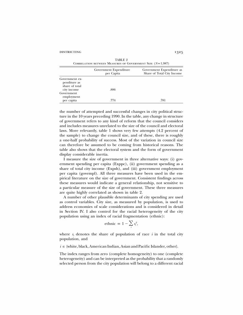
TABLE 2Correlation between Measures of Government Size (Np1,987)
Government Expenditureper Capita
Government Expenditure asShare of Total City Income
Government ex-penditure asshare of totalcity income .886
Governmentemploymentper capita .774 .781
the number of attempted and successful changes in city political struc-ture in the 10 years preceding 1990. In the table, any change in structureof government refers to any kind of reform that the council considersand includes measures unrelated to the size of the council and electorallaws. More relevantly, table 1 shows very few attempts (4.2 percent ofthe sample) to change the council size, and of these, there is roughlya one-half probability of success. Most of the variation in council sizecan therefore be assumed to be coming from historical reasons. Thetable also shows that the electoral system and the form of governmentdisplay considerable inertia.
I measure the size of government in three alternative ways: (i) gov-ernment spending per capita (Exppc), (ii) government spending as ashare of total city income (Expsh), and (iii) government employmentper capita (govempl). All three measures have been used in the em-pirical literature on the size of government. Consistent findings acrossthese measures would indicate a general relationship, not sensitive toa particular measure of the size of government. These three measuresare quite highly correlated as shown in table 2.
A number of other plausible determinants of city spending are usedas control variables. City size, as measured by population, is used toaddress economies of scale considerations and is considered in detailin Section IV. I also control for the racial heterogeneity of the citypopulation using an index of racial fragmentation (ethnic):
2ethnic p 1 � s ,� ii
where si denotes the share of population of race i in the total citypopulation, and
i � {white, black, American Indian, Asian and Pacific Islander, other}.
The index ranges from zero (complete homogeneity) to one (completeheterogeneity) and can be interpreted as the probability that a randomlyselected person from the city population will belong to a different racial

1326 journal of political economy
group than another randomly selected person. The racial categories aretaken from the 1990 census. In the sensitivity analysis, I also control fora similar measure of heterogeneity for the council, using data on councilmembers by race. The additional control variables are per capita income(incomepc), educational attainment as measured by the percentage ofpopulation with a bachelor of arts or higher degree (BAgrad), andincome inequality in the city as measured by the ratio of the mean tomedian household income (MMI90).12 Income and educational attain-ment are likely determinants of the demand for public services. Theinequality variable is included since the size of government may respondto redistributive pressure arising out of income inequality. Table 3 showsthe summary statistics on all the variables used in the study.
It is useful to consider what drives the variation of council size in thesample. Theoretically, the most obvious determinant is city population.Bigger jurisdictions should, and do, have bigger councils. Regressingcouncil size on city population (in millions) yields the following equa-tion (standard errors are in parentheses):
2Csize p 6.62 � 5.36Pop90, R p .15, N p 1,972.(0.07) (0.29)
The slope coefficient indicates that although bigger cities have biggercouncils, the effect is considerably small in magnitude. An increase inthe city population from 10,000 to 100,000 would be associated with anincrease in the council size from 6.7 to 7.2—a fairly small effect.13 Thesmall magnitude of effect is consistent with the evidence on the infre-quency of changes in council size: over time, while city populations mayhave changed considerably, council size has changed less frequently,leading to a small slope coefficient in the 1990 cross section. The otherimportant sample correlates of council size are the state in which thecity is located and the city’s ethnic and income heterogeneity. Statematters because city councils derive their authority from state govern-ments, which vary in their laws governing local governments. Runningthe regression above with a complete list of state indicator variablesyields an adjusted of .41, whereas the estimated coefficient on pop-2Rulation remains virtually unchanged (and highly significant). To theextent that preferences for public services are correlated along ethnic
12 For a subset of the sample I had data on the income-based Gini coefficient and onthe city unemployment rate. The findings on inequality are robust to either measure used.The unemployment variable was used to control for government spending responding tounemployment for standard Keynesian reasons. The results on council size were robustto including the unemployment rate in the regression.
13 The same equation estimated in log-log form yields an elasticity of council size withrespect to city population of 0.11. Taagepera and Shugart (1989, chap. 5) estimate a similarequation for a cross section of countries in 1985 and report an elasticity of legislature size(lower house) with respect to country population of 0.33.

TABLE 3Summary Statistics
Variable Units Minimum Maximum Median MeanStandardDeviation
Number ofObservations
City government expenditures per capita $1,000 per capita .020 7.836 .641 .791 .539 1,991City government expenditures, as a percentage
of total city income Percentage .078 44.660 4.933 5.973 4.123 1,991City government employees per capita Employees per 1,000 population .429 98.873 9.746 12.101 8.835 1,996Council size Number of people 3 50 6 6.859 2.888 2,342Council size, 1960 Number of people 5 9 7 6.505 1.517 465Ethnic Fraction .004 .730 .187 .235 .173 3,146Council-ethnic Fraction 0 .720 0 .122 .180 1,779City population Number of people 10,005 7,322,564 21,099 45,540 173,103 3,146Income per capita $10,000 per capita .438 6.330 1.386 1.528 .597 3,146%BAgrad Fraction .007 .909 .188 .225 .129 3,146Ratio of mean to median household income Ratio .986 4.777 1.213 1.248 .185 3,146Council members elected by district Number of people 0 50 0 2.856 4.048 2,342Council members elected at large Number of people 0 16 5 4.003 2.731 2,342Mayor-council form of government Indicator variable 0 1 0 .378 .485 1,696Mayor-council form of government, 1960 Indicator variable 0 1 0 .359 .480 473Mayor elected directly from city population Indicator variable 0 1 1 .775 .417 1,696Mayor proposed budget to council Indicator variable 0 1 0 .173 .378 1,696Mayor appoints department heads Indicator variable 0 1 0 .232 .422 1,696Mayor can veto council-passed measures Indicator variable 0 1 0 .345 .475 1,696Mayor can veto specific items of appropriations Indicator variable 0 1 0 .086 .281 1,696
Source.—The 1992 Census of Governments; 1990 Census of Population; 1992 Census of Governments, Government Organization File (all Census Department); a survey of citygovernments conducted by the ICMA; and the County and City Compendium 1993 (Slater-Hall Information Products, Washington, DC).
Note.—Cross-sectional city government data pertain to 1990, unless otherwise stated. Ethnic is an index of racial heterogeneity for the city population, ranging from zero (leastheterogeneity) to one (most heterogeneity). Its construction is described in the text. Council-ethnic is a similar measure for the city council using data on council members byrace. %BAgrad is the percentage population over 25 with a college or higher educational degree. For the indicator variables, the variable equals one (and zero otherwise) if thecorresponding statement is true. The last five variables on the powers of mayors are classified further in table 9 below. The text provides further details on all variables.

1328 journal of political economy
and income lines, we should expect greater demand for political rep-resentation in more heterogeneous jurisdictions for a given population.Regressing council size on population and two measures of heteroge-neity (ethnic, as defined above, and income inequality, measured by theratio of the mean to median income) as well as a complete list of stateindicator variables gives
Csize p 5.87 � 5.22Pop90 � 1.64ethnic � 1.02MMI,(0.25) (0.39) (0.40)
2R p .42, N p 1,972.
The regressions for government size reported below control for thesemeasures of income and ethnic heterogeneity, and the coefficients onthese variables can be interpreted as capturing their direct impact ongovernment size, when the effects that may go through council size arecontrolled for.
IV. Results I: Districting and Government Size
Table 4 presents the results of ordinary least squares (OLS) regressionsfor the size of government on the size of the city council and othervariables. The three measures of government size are used in log formbecause of the presence of large outliers in each of these series andbecause in this form the coefficients on the council size variable canconveniently be interpreted as the elasticity of government size withrespect to the number of electoral districts. The first specification in-cludes only city population as a control variable. Subsequent specifi-cations play close attention to the following sets of factors: (i) otherplausible determinants of government size, (ii) the nonlinear effects ofcity population on government size, and (iii) the presence of state-specific effects correlated with both council size and government size.I discuss each in turn below.
The first specification indicates that the magnitude of effect of councilsize on government size is close across the three measures of governmentsize. When the control variables are added in the second specification,these magnitudes remain relatively unchanged, indicating, in particular,that the council size effect is not going through two other possiblepolitical factors: racial heterogeneity and income inequality. Coefficientson the control variables indicate that government size increases withthe racial heterogeneity of the city and the ratio of mean to medianincome of the city. The first of these two findings is consistent with theresults in Alesina, Baqir, and Easterly (1999) and is not explored furtherhere except to note that since the index of racial fragmentation goesup with the effective number of racial groups in the population, it is
districting 1329
important to determine whether bigger councils might simply be prox-ying for a more heterogeneous population. Results discussed in sub-section E below indicate that this is not the case. The positive coefficienton the measure of income inequality interestingly relates to a long-standing literature on the relationship between income inequality andredistributive spending.14 The coefficient on per capita income is con-sistent with previous studies of local public goods that find the demandfor local public services to be income inelastic.15 Plausible coefficientson the control variables suggest that the empirical model is not grosslymisspecified.
A. City Size
The variable with the greatest statistical significance is the logarithm ofthe city population. Log form was used to capture the presence ofoutliers in the series. Since city size is strongly correlated with govern-ment expenditures and council size, the third specification splits the1990 population into five quintiles and allows for a different slope co-efficient for each interval. The results are illuminating. In small andmedium-sized cities, per capita government expenditures decline withcity population, consistent with the presence of economies of scale. Anincrease of 10,000 people in the city population for cities at the smallestquintile is associated with approximately an 18 percent decrease in ex-penditures per capita—an effect of considerable magnitude. At higherpopulation quintiles the estimated effect becomes weaker in magnitude,eventually turning positive for the very biggest cities, suggesting theyielding of economies of scale to diseconomies.16 The pattern of coef-ficients suggests a U-shaped relationship between the size of governmentand city population. Figure 1, which makes a finer division of city sizesin the sample, confirms this. The vertical bars show average per capitagovernment expenditures by decile of the city population.17 The con-nected line shows the average residuals by population decile from aregression of per capita expenditures on all the other variables includedin table 4. Both series show a similar pattern and suggest that economiesof scale in government spending eventually yield to diseconomies of
14 See Benabou (1996) for an excellent review of this literature. This relationship is notexplored further here since it is not the focus of the paper, but the findings on this variableare consistent in all the specifications.
15 See, e.g., the review provided by Mueller (1987).16 The F-tests for the equality of coefficients across the five population quintiles reject
at p-values of less than .001.17 The pattern is not markedly different when median per capita expenditure for the
interval is used instead of the mean. Figures for the other two measures of governmentsize yield very similar results.

1330
TABLE 4OLS Regressions for Government Size
(1) (2) (3) (4)
A. ln(Government Expenditures per Capita)
ln(council size) .2760***(.0384)
.3021***(.0383)
.3203***(.0384)
.1127***(.0373)
ln(city population) .1515***(.0133)
.1307***(.0139)
Ethnic .1920**(.079)
.2550***(.0783)
.5099***(.0911)
Income per capita .2272***(.0355)
.2339***(.0359)
.1631***(.0349)
%BAgrad �.6060***(.1537)
�.5940***(.1557)
�.3898***(.1425)
Mean/median income .6613***(.0921)
.6543***(.0939)
.8524***(.0957)
City population:1st quintile �1.8201***
(.3143)�1.2740***
(.2821)2d quintile �1.2652***
(.2057)�.9433***(.1796)
3d quintile �.7196***(.1425)
�.5609***(.122)
4th quintile �.2002**(.0808)
�.1842***(.0691)
5th quintile .0147***(.0047)
.0188***(.0049)
Constant �2.4819***(.1436)
�3.3969***(.1825)
�1.9632***(.139)
�.0401(.1633)
State fixed effects no no no yesObservations 1,972 1,972 1,972 1,972Adjusted 2R .10 .15 .14 .39Standard error of
regression .536 .523 .525 .442
B. ln(Government Expenditures as a Share of Income)
ln(council size) .2855***(.0393)
.2746***(.0369)
.2903***(.037)
.1100***(.0367)
ln(city population) .1225***(.014)
.1058***(.0136)
Ethnic .2791***(.0772)
.3357***(.0767)
.5955***(.0901)
Income per capita �.2913***(.0338)
�.2852***(.0339)
�.3332***(.0343)
%BAgrad �.7339***(.1497)
�.7187***(.1515)
�.5896***(.1415)
Mean/median income .9025***(.0917)
.8921***(.0937)
1.0982***(.097)
City population:1st quintile �1.3642***
(.3061)�.7671***(.2778)
2d quintile �1.0219***(.201)
�.6553***(.1771)
3d quintile �.6137***(.1377)
�.4491***(.1194)
4th quintile �.1694**(.0789)
�.1437**(.0679)

1331
TABLE 4(Continued)
(1) (2) (3) (4)
5th quintile .0123***(.0047)
.0154***(.0045)
Constant �.193(.1494)
�.6216***(.1804)
.5390***(.138)
2.2141***(.1669)
State fixed effects no no no yesObservations 1,972 1,972 1,972 1,972Adjusted 2R .07 .28 .28 .45Standard error of
regression .578 .508 .510 .434
C. ln(Government Employment per Capita)
ln(council size) .5082***(.042)
.4998***(.0407)
.4950***(.0408)
.1322***(.0374)
ln(city population) .0345**(.0146)
.0226(.0146)
Ethnic .0702(.0889)
.0678(.0887)
.3166***(.0892)
Income per capita �.0375(.0376)
�.0358(.0375)
.0081(.037)
%BAgrad �.5437***(.174)
�.5205***(.1749)
�.4514***(.1561)
Mean/median income 1.4238***(.1079)
1.4157***(.1095)
1.1636***(.1047)
City population:1st quintile �.357
(.3331)�.5887**(.2865)
2d quintile �.2609(.2278)
�.4923***(.1883)
3d quintile �.3917**(.152)
�.4735***(.1179)
4th quintile �.1462(.0941)
�.1513**(.0714)
5th quintile .0032(.0054)
.0159***(.003)
Constant .9901***(.1544)
�.5121***(.1984)
�.2178(.1573)
2.1450***(.1772)
State fixed effects no no no yesObservations 1,977 1,977 1,968 1,968Adjusted 2R .08 .20 .20 .51Standard error of
regression .590 .551 .552 .432
Note.—The dependent variable for each measure of government size is named in each panel. The first specificationfor each measure includes only council size and the natural logarithm of the city population. The last specification foreach measure includes all listed covariates and a complete set of state fixed effects. Ethnic is an index of racialheterogeneity for the city population: higher values represent greater heterogeneity. %BAgrad is the percentage ofpopulation over 25 with a college or higher degree. All variables are described in table 3. Population quintiles havepopulation data expressed in 100,000s. The data set is a 1990 cross section of city governments in the United States,and sources are described in Sec. III in the text. Robust standard errors are in parentheses.
** Significant at the 5 percent level.*** Significant at the 1 percent level.

1332 journal of political economy
Fig. 1.—Government size by city size
scale. The estimated relationship with respect to council size is notaffected when we allow nonlinear effects of population size.
B. State-Specific Effects
Since state-specific factors, such as differing degrees of state fiscal de-centralization, are likely to affect both local government spending andlocal political structure, the fourth specification in table 4 controls fora complete set of state fixed effects. The estimated coefficient on councilsize drops to little over a third of its value. Figure 2 plots the logarithmof the median per capita city expenditure in a state against the mediancouncil size in the state and shows a strong positive correlation.18 Note,however, the presence of influential observations: Washington, D.C.(with one local government) and the New England states are clusteredon the upper-right side of the figure (fig. 3 excludes these states). Wash-ington, being the nation’s capital and having the highest level of ex-penditures per capita, can deserve special treatment. The New Englandstates are the oldest states in the United States with a history of liberaland very democratic local government traditions. Some cities in theNew England states also use the town meeting form of local government,which is unique to these states. A closer examination shows that thereduction in the council size coefficient in the fourth specification is
18 Figures using the other two measures of government size look very similar.

districting 1333
Fig. 2.—Council size and government expenditures: all states
accounted for by the New England effect. Running the fourth specifi-cation with only the indicators for the New England states gives closeto the same reduction in the coefficient on council size.19 The resultsare presented in row 1a of table 5. An F-test for the equality of thecoefficients on the six state indicators does not reject at conventionallevels, indicating that we could include one indicator variable for NewEngland states. Row 1b of table 5, which reports the coefficients andstandard errors on the council size variable when only this indicator isincluded in the equation, confirms this. Does the relationship betweencouncil size and government expenditures survive when we look onlyat the non–New England states? The subsequent two rows in table 5show that it does. Row 1c reports the coefficients when only non–NewEngland states are included in the sample and state indicators are notincluded. The estimated coefficient for each measure of governmentsize is very close to the full sample regression with all state indicators(col. 4 of table 4). Moreover, inclusion of state indicators in thisnon–New England sample (row 1d of table 5) does not alter the coef-ficient much for two of the three measures of government size, consis-tent with the discussion above that the original reduction in the coef-
19 The New England states are Connecticut, Maine, Massachusetts, New Hampshire,Rhode Island, and Vermont. The same holds if we include in addition an indicator forWashington, D.C.

1334 journal of political economy
Fig. 3.—Council size and government expenditures: excluding Washington, D.C., andNew England.
ficient was coming from the New England states.20 Table 5 also pullstogether results from other specification tests, which are discussed indetail below.
C. Reverse Causality
Evidence presented in Section III suggested that council size is costlyto change, which should limit concerns that results are contaminatedbecause of reverse causation. However, it is possible that over long pe-riods, council size may have adjusted to incorporate spending prefer-ences of cities.21 To address these concerns, I present results with in-strumental variables, using the size of the city council in 1960 as aninstrument.22 Since we are going a fairly long period back in time, thisvariable is likely exogenous to the spending decisions in 1990. However,
20 There are only 92 observations if we look at the New England sample. Regressionsfor government size in this sample do not give any significant variable except racial het-erogeneity. Note that even population is not significant, which indicates a not very goodfit of the model.
21 It is, though, not clear why greater government spending would require bigger coun-cils. The council refers to the legislative function in government, whereas governmentprograms typically fall under the executive branch. Getting more government programsis more likely to mean more government employees than more legislators.
22 The data come from Aiken and Alford (1972) and were obtained electronically fromthe web site of the Inter-university Consortium for Political and Social Research, http://www.icpsr.umich.edu, study 0028.

TABLE 5Sensitivity Analysis
Coefficient on ln(Council Size) When the De-pendent Variable Is:
ln(Expenditureper Capita)
ln(Expendituresas Share of
City Income)
ln(GovernmentEmploymentper Capita)
0. Baseline coefficient .1127(.037)
.1100(.037)
.1322(.037)
1. State-specific effects:a. Indicators only for New England states .1284
(.039).1115
(.038).2982
(.041)b. One indicator for New England .1323
(.038).1147
(.038).2937
(.040)c. Non–New England sample, without state
indicators.1410
(.041).1224
(.040).3218
(.043)d. Non–New England sample, with state
indicators.1294
(.043).1255
(.042).1496
(.042))e. State share in total revenue, with all state
indicators.1200
(.038).1169
(.037).1366
(.038)2. Population growth, 1980–90 .0971
(.038).0972
(.037).1051
(.037)3. Effective number of ethnic groups .1088
(.049).1114
(.047).1378
(.049)4. Ethnic heterogeneity:
a. Ethnic ≥ median (.20) .1374(.039)
.1275(.038)
.1470(.039)
b. Ethnic ! median .0879(.039)
.0924(.038)
.1173(.039)
5. Big councils vs. small councils:a. Council size 1 9 .1361
(.04).1338
(.039).1510
(.041)b. Council size ≤ 9 .1718
(.049).1703
(.048).1797
(.052)6. Big cities vs. small cities:
a. City population ≥ median (25,555) .1294(.038)
.1266(.037)
.1381(.038)
b. City population ! median .0756a
(.040).0730a
(.039).1191
(.04)7. Central vs. suburban cities (includes indica-
tors for central and suburban cities).1464
(.047).1402
(.045).1955
(.048)8. Population density: controls for
ln(population density).1114
(.037).1084
(.037).1308
(.038)9. Percentage voting for Democratic president .1144
(.039).1102
(.039).1340
(.039)
Note.— The table reports results from variations on the fourth specification in table 4 for each measure of governmentsize. Row 0 reproduces the original specification for ease of reference. Only the coefficients (and robust standard errorsin parentheses) on the council size are reported to conserve space. Results on the other variables are discussed in Sec.IVE. Each regression additionally includes all variables of table 4, including population quintiles and state indicators.Effective number of ethnic groups equals the reciprocal of one minus the racial heterogeneity variable for the citycouncil. For rows 4–6, the council size variable is split according to the conditions in the two subrows. Numbers ofobservations range from 1,455 to 1,972 depending on data availability for the additional variables.
a p-value !.06 (for all other estimated coefficients associated p-values ! .05).

1336 journal of political economy
it is available for only 465 cities of the OLS sample. Since there is aconsiderable change in the sample size, table 6 first reports the OLSand then the two-state least-squares (2SLS) results (both with and with-out the state indicators). The OLS results show that the statisticallysignificant estimated coefficients (on council size, racial heterogeneity,per capita income, and the ratio of mean to median income) are quiteclose to the estimates in the full sample of table 4. Thus the 465-observation sample is representative of the full sample. When we in-strument for the 1990 value of council size, the estimated coefficientincreases in magnitude. If reverse causality was contaminating the OLSresults, we would have expected a reduction in the coefficient with theinstrumental variable specification. One explanation that can accountfor the increase is that, over time, cities that have received net populationinflows would have benefited from economies of scale in governmentspending while at the same time would have been under pressure toincrease representation of the council. This would lead to a downwardbias in the 1990 cross-sectional relationship between council size andgovernment spending, and the instrumental variable results help torecover the causal effect of districting on spending.
D. Discussion
Given these results, it is useful to consider the magnitude of the effectof council size on government size. Focusing on per capita expendituresand using the baseline specification of column 4 of table 4, we can take0.11 as an estimate of the magnitude of effect. An addition of onecouncil member, then, to an average city council (of seven members)would be associated with a 1.6 percent increase in per1(≈ 0.11 # )
7capita city government expenditures. Given average per capita cityspending of $792, this amounts to an increase of $12 per capita. Inaggregate terms, these coefficients imply that for an average city of58,000 people, an addition of one political district in the city would beassociated with an increase of $0.72 million (≈ 0.016 # 792 # 58,000)in the city budget.23 With a median city budget of $17.5 million, andgiven that when cities consider changes in the number of seats in the
23 If anything, this estimate is likely to be an underestimate of the effect on aggregateexpenditures. Redoing the regressions with the log of total city government expendituresas the dependent variable gives an estimated coefficient (standard error) of (i) 0.294(0.061) in the OLS regression of table 4 (with state indicators), (ii) 0.353 (0.191) in the2SLS specification of table 6 (with state indicators), and 0.381 (0.090) in the OLS re-gression corresponding to panel B of table 10 below with indicators and interaction forcities with strong mayors. When the smallest of these coefficients (0.29) is used, theestimated effect of an increase of one councilman on the aggregate budget is $3.1 millionat the sample mean and $0.73 million at the sample median of total expenditures.

districting 1337
city council they typically consider changes of more than one council-man, these are fairly substantial effects.
It is also useful to consider actual government spending in otherwisesimilar cities that have very different council sizes. Two of the key de-terminants of council size are state and population. Grouping big citiesby state and population and looking for big differences in council sizesgives an illustrative example from Connecticut. Bridgeport and NewHaven had very similar levels of population (142,000 and 130,000, re-spectively), racial heterogeneity (0.571 and 0.573), per capita income($13,100 and $12,970), land area (16 and 19 square miles), and otherindicators in 1990 used in the baseline regression. New Haven, however,has 30 council members, 10 more than Bridgeport. In 1990 it also spent$600 more than Bridgeport. The predicted difference from the regres-sion in per capita spending is $200 for these two cities.
E. Additional Sensitivity Analysis
In the rest of this section I present results from other sensitivity analysisexercises carried out to check the robustness of the basic results. Table5 pulls together the results from variations on the basic specification ofcolumn 4 of table 4.24 For ease of reference, row 0 repeats the resultsfrom table 4. The subsequent four rows were discussed above in thecontext of state-specific effects. Row 1e presents one additional speci-fication to control for state-specific effects: it controls for the share oftotal revenue coming from state government as a proxy for the degreeof state influence in the fiscal affairs of the city. This share varies in thesample from zero to 88 percent with a mean (median) share of 16percent (13 percent). Row 1e shows that the council size coefficients donot change much when we control for this variable. It is important tonote that for a good fit between theory and data, most of the revenueneeds to come from local sources. If most revenues came from, say, thestate government and cities lobbied to get greater revenues transferreddown, the appropriate measure of the “number of players” in the com-mon pool would be the number of municipal governments in the state.For the average city, 78 percent of the revenue comes from local sources(median 81 percent). As a final check, I ran the basic regression oftable 5 with the log of the locally generated per capita governmentrevenue as the dependent variable. The estimated coefficient (standarderror) on ln(council size) is 0.0856 (0.038) with a p-value of .024, veryclose to the original estimates of the effect on the size of government.
24 Coefficients on the control variables are suppressed to conserve space. Significantdifferences in any of these variables are noted in the discussion. Complete results areavailable on request.

1338
TABLE 62SLS Results for Government Size (Np465)
(1) (2) (3) (4)
A. ln(Government Expenditures per Capita)
Estimation OLS 2SLS OLS 2SLSState fixed
effects no no yes yesln(council size) .4084***
(.0832).6448***
(.1319).1630**
(.0751).3173**
(.147)Ethnic .2327*
(.1379).3013**
(.1422).4237***
(.1361).4188***
(.1369)Income per
capita.2496***
(.0627).2716***
(.064).1788***
(.0527).1796***
(.053)%BAgrad .1634
(.294).1233
(.2971).2781
(.2277).2754
(.2288)Mean/median
income.4021**
(.1883).4069**
(.19).6143***
(.1558).6093***
(.1566)City population:
1st quintile �.7590**(.3126)
�.7671**(.3154)
�.5950**(.238)
�.5805**(.2395)
2d quintile �.2626(.2015)
�.2675(.2033)
�.1823(.1516)
�.177(.1524)
3d quintile �.4312***(.1395)
�.4429***(.1408)
�.2719***(.1042)
�.2804***(.105)
4th quintile �.1957**(.0883)
�.2023**(.0891)
�.0421(.0671)
�.053(.068)
5th quintile �.0012(.0192)
�.0154(.0203)
.0275*(.0148)
.0182(.0167)
Constant �1.7937***(.3001)
�2.2838***(.369)
�1.6949***(.4203)
�2.0302***(.5036)
Adjusted 2R .16 .15 .57 .57Standard error
of regression .474 .478 .338 .340
B. ln(Government Expenditures as a Share of Income)
Estimation OLS 2SLS OLS 2SLSState fixed
effects no no yes yesln(council size) .3956***
(.0799).6060***
(.1265).1684**
(.0739).2996**
(.1444)Ethnic .2595*
(.1323).3205**
(.1363).4687***
(.1339).4645***
(.1345)Income per
capita�.2502***(.0602)
�.2307***(.0613)
�.3066***(.0518)
�.3060***(.052)
%BAgrad �.1809(.2822)
�.2166(.2848)
�.1271(.224)
�.1295(.2249)
Mean/medianincome
.7334***(.1807)
.7377***(.1821)
.9781***(.1533)
.9738***(.1539)
City population:1st quintile �.6901**
(.3)�.6973**(.3023)
�.5116**(.2342)
�.4993**(.2354)
2d quintile �.2486(.1934)
�.2529(.1949)
�.161(.1492)
�.1566(.1498)
3d quintile �.4062***(.1339)
�.4166***(.135)
�.2542**(.1025)
�.2614**(.1032)
4th quintile �.1853**(.0847)
�.1912**(.0854)
�.0432(.066)
�.0525(.0668)

1339
TABLE 6(Continued)
(1) (2) (3) (4)
5th quintile �.0043(.0184)
�.0169(.0195)
.0209(.0145)
.013(.0164)
Constant .5793**(.2881)
.1431(.3538)
.6093(.4136)
.3242(.4948)
Observations 465 465 465 465Adjusted 2R .20 .19 .57 .57Standard error
of regression .455 .458 .333 .334
C. ln(Government Employment per Capita)
Estimation OLS 2SLS OLS 2SLSState fixed
effects no no yes yesln(council size) .6965***
(.0894).9087***
(.1413).2104***
(.074).3545**
(.1446)Ethnic .0629
(.148).1244
(.1523).3039**
(.134).2993**
(.1347)Income per
capita�.046(.0673)
�.0263(.0685)
.0396(.0519)
.0403(.0521)
%BAgrad .4991(.3157)
.4631(.3182)
.4785**(.2241)
�.4759**(.2252)
Mean/medianincome
1.0453***(.2022)
1.0496***(.2035)
.7374***(.1534)
.7326***(.1541)
City population:1st quintile �.6291*
(.3357)�.6364*(.3378)
�.4531*(.2343)
�.4396*(.2357)
2d quintile �.0984(.2163)
�.1028(.2177)
�.0342(.1492)
�.0294(.15)
3d quintile �.3780**(.1498)
�.3885**(.1508)
�.1662(.1026)
�.1741*(.1033)
4th quintile �.2024**(.0948)
�.2083**(.0954)
.0177(.066)
.0075(.0669)
5th quintile �.0376(.0206)
�.0504**(.0218)
.0057(.0146)
�.003(.0164)
Constant �.1096(.3223)
�.5494(.3953)
.9063**(.4138)
.5933(.4955)
Observations 465 465 465 465Adjusted 2R .19 .18 .65 .65Standard error
of regression .509 .512 .333 .335
Note.—For each measure of government size and for specifications with and without a complete set of state indicators,the table compares the results of OLS and 2SLS regressions. Council size (in 1990) is instrumented with 1960 councilsize using historical data from Aiken and Alford (1972). The OLS results are reported since the common sample ismuch smaller than the regressions of table 4 because of availability of 1960 council size data. Population quintiles havepopulation data expressed in 100,000s. Robust standard errors are in parentheses.
* Significant at the 10 percent level.** Significant at the 5 percent level.*** Significant at the 1 percent level.

1340 journal of political economy
Row 2 of table 5 includes as an additional regressor the growth inthe city population, which can be an important factor because of theimplications for city infrastructure. The estimated coefficient on thepopulation growth variable is negative (�0.202 for the expenditure percapita regression) and statistically significant. When I split the popu-lation growth variable in a manner similar to the 1990 population var-iable as described above, I find that most of the effect is coming fromthe upper quintiles: the coefficients on the first three quintiles of pop-ulation growth are not significant, whereas there is very little change inthe coefficients on other variables. The negative estimated effect is there-fore coming from rapidly growing cities in the sample.
Although we control for racial heterogeneity of the city, heterogeneityof the council may be an additional factor affecting government spend-ing. On the one hand, one could envisage that it is not council size perse but the number of racial groups in the city council that, potentiallythrough a similar common-pool type argument, is driving up govern-ment expenditures. Since bigger councils are likely to be more heter-ogeneous, council size may simply be proxying for the number of racialgroups in the council. This would imply that government spendingshould not be related to the number of districts in racially homogeneouscouncils. On the other hand, one could argue that in addition to elec-toral districts, spending coalitions get formed along racial groups, sothat spending is sensitive to both the number of districts and the numberof racial groups in the council. Row 3 presents the results when weadditionally control for a measure of the effective number of racialgroups in the council.25 There is very little impact on the coefficient forthe council size variable. In addition, the coefficient on the effectivenumber of ethnic groups variable ranges between 0.10 and 0.12 for thethree specifications and is significant at 5 percent. These results aremore consistent with the latter interpretation: it is not the case that thesize of the council is simply proxying for the ethnic heterogeneity ofthe council. The next two rows (4a and 4b) show separate slope coef-ficients for heterogeneous and homogeneous cities and provide furtherevidence that the effect of districting is present in both.
In the government expenditure regressions, 1,777 of the 1,972 citiesin the sample have councils composed of nine or fewer members. To
25 This is in addition to controlling for the racial heterogeneity of the city population.The effective number of ethnic groups is the reciprocal of one minus the ethnic variablefor the city council using data on council members by race. When racial groups aredistributed equally, this equals the number of racial groups. When groups are not dis-tributed symmetrically, as in one large group and several small groups, it is less than thenumber of groups to capture the “effective” number of groups. This is the same variableused by, e.g., Taagepera and Shugart (1989), Ordeshook and Shvetsova (1994), and Cox(1997) in their studies of the effects of electoral systems on the number of effective partiesin the legislature.

districting 1341
see whether the relationship holds separately in big and small councils,I estimate separate coefficients on council size for these two groups.Row 5 shows significant effects for both large and small councils. I alsoestimate separate coefficients depending on whether the city populationis less than or greater than the median for the sample (25,555). Thisis done partly to capture the commonly discussed idea that big citieshave their special problems and may attain poorer outcomes for reasonsother than the externalities inherent in distributive politics. Results showthat (a) the magnitude of the effect is stronger in large cities, and (b)the statistical significance for the council size variable in small citiesdrops somewhat, but the coefficients are significant at 6 percent for twoof the three measures and at 5 percent for the third measure of gov-ernment size.
The next two regressions include other potentially omitted variables:inner-city versus suburban versus rural cities and population density.There may be systematic differences between inner cities and suburbsthat are correlated with both desired government expenditures andcouncil size. Central city residents typically favor greater public servicesand, because they are more heterogeneous, may also desire bigger citycouncils. Suburbs generally have the opposite characteristics. The sameeffect to some extent can be picked up in the population density var-iable. Results show that the council size effect is robust to these con-siderations. I also try to control directly for variation in political pref-erences by using data on percentages voting for a Democratic presidentin the 1992 presidential election, assuming that, though many factorsare likely to affect a voting decision, residents with innate preferencesfor big government are, ceteris paribus, more likely to vote for a Dem-ocratic candidate. Such voting data are available only at the county level.I mapped each city in the sample to the county it is located in and usedthe county electoral data as a proxy for the city electoral variable.26 Theresults after I control for this variable are shown in row 9 of table 5.There is little change for the council size coefficient, and, interestingly,the coefficient on the voting variable is not significant in any of thespecifications, suggesting that other controls in the equation may alreadybe accounting for the variation in political preferences.
V. Results II: Electoral Systems and Form of Government
Table 1 demonstrated that the city electoral system and form of gov-ernment change relatively infrequently. The purpose of this section is
26 For this to be a good proxy, it requires that there be a relatively high correlationacross cities in a county on voting patterns. In the absence of direct information on howlarge or small this variation may be, the results on this variable should be interpreted withcaution.
1342 journal of political economy
to examine whether the relationship between council size and govern-ment size varies systematically across these two sets of politicalinstitutions.
A. Electoral Systems
The key variation in electoral systems across cities is whether candidatesare elected from the entire city or from districts within the city.27 Of thetotal number of cities in the sample, 56 percent have at-large systems,17 percent have district systems, and the remaining 27 percent have amixed system in which some council members are elected by districtand some at large.28 Traditionally cities had district-based systems. At-large systems were introduced in some cities around the turn of the lastcentury in part because it was believed that they would help to curtailpork barrel–type spending by inducing council members to treat theentire city as their constituency. For instance, Richard S. Childs, an earlymunicipal reformer, noted the following as a criticism of ward systems(and a recommendation for at-large systems): “ward elections notori-ously produced political small fry who intrigued in the council for pettyfavors and sought appropriations for their wards in reckless disregardof city-wide interests and the total budget” (1965, p. 37). In their reviewof the argument for adopting at-large systems in U.S. cities, Engstromand McDonald (1986) note that council members elected at large were“expected to make decisions on the basis of what they perceived to begood for the entire city, not just one geographic or social segment ofit” (p. 203).
Alternatively, at-large council members, despite running from thewhole city, may have “home bases” or particular constituencies com-prising subsets of the city population that they seek to distribute ex-penditures to in exchange for votes.29 If so, we would expect the sameeffect from increasing at-large council members as from increasing dis-trict council members: an additional at-large council member represents
27 I have so far been using the terms “council size” and “number of districts” inter-changeably. The two need not be the same in cities in which some council members areelected at large. The results in this section will justify the use of council size as the relevantright-hand-side variable.
28 For most cities, when council members are elected at large, they run from the entirecity. A few cities, however, have several multimember districts. Although I do not have thedata to distinguish between single-member and multimember district systems, Welch(1990) collected these data in a survey and found that 1.9 percent of her sample weresuch cities. For empirical purposes, therefore, I take the district electoral systems to meansingle-member district systems.
29 See Uslaner (1985) for a study of Israel’s Knesset, an extreme example of an at-largesystem at the national level in which all representatives are elected from the entire country.He shows that legislators identify themselves with particular constituencies within thecountry along geographical, ethnic, and religious lines.

districting 1343
an additional player in the pool. Such home bases can develop alongdimensions such as ethnicity, income, age, and any other characteristicthat can segment the city population. Indeed, in at-large electoral sys-tems, geography may be one of the dimensions along which constitu-encies for individual council members may form. It will be useful toexplicitly state the two contrasting views on the role of at-large councilmembers.
Hypothesis I. At-large council members cater to the common goodof the whole city, and district council members cater to the good oftheir respective districts.
Hypothesis II. At-large council members cater to particular constit-uencies and face the same asymmetry between benefits and costs oftheir policy proposals as district council members.
The prediction to be tested is whether the relationship between coun-cil size and government size is nonexistent in cities with at-large councilmembers. As a first look at the question, I estimate the following spec-ification:
ln (g) p a � a D � a ln ( J ) � a D 7 ln ( J ) � b 7 Z � e,0 1 L 2 3 L
where g is a measure of the size of government, DL is an indicator variablefor a council with a majority of the council elected at large, J is the sizeof the council, and Z are all controls used in table 4. The predictionsof hypothesis I are and and those of hypothesis IIa 1 0 a � a p 0,2 2 3
are anda 1 0 a p 0.2 3
The differing predictions rest on the estimated coefficient for a3.Results, presented in panel A of table 7, show that the data reject thefirst hypothesis for all three measures of government size. For the gov-ernment expenditure regressions, the estimate of a3 is not statisticallydifferent from zero, indicating the same relationship between districtingand government size in both district and at-large majority councils. Forthe government employment regression, an at-large majority council isassociated with a negative intercept effect but a steeper positive rela-tionship between council size and government size. At the sample mean,the net effect of switching to an at-large majority council is an increasein government size of 15 percent. The coefficients on the other variablesare suppressed to conserve space, but they are close to the estimates intable 4.
Panel B of table 7 takes a closer look at the data. The specificationabove lumped together pure at-large systems with those mixed systemsin which a majority of the council members were elected at large. Thispanel separates the coefficients across nonmixed and mixed electoralsystems. The first three coefficients compare cities with district systemsto at-large systems, and the next three coefficients compare mixed sys-tems with an at-large majority to mixed systems with a district majority.

TABLE 7Regressions for Effects of Electoral Systems
ln(Expendituresper Capita)(Np1,972)
ln(Expendituresas Share of
City Income)(Np1,972)
ln(GovernmentEmploymentper Capita)(Np1,968)
Panel A
Majority at large �.2056(.1358)
�.1848(.1316)
�.4662***(.1442)
ln[council size (J)] .1510***(.0507)
.1475***(.0493)
.1252**(.0504)
Majority at large#ln(J) .075(.0709)
.0701(.0686)
.2051***(.0759)
Adjusted 2R .33 .43 .45
Panel B
Pure#majority at large �.1457(.1399)
�.1324(.1358)
�.3717**(.1474)
Pure#ln(J) .1132**(.0495)
.1107**(.0483)
.0957*(.05)
Pure#majority at large#ln(J)
.0735(.0737)
.0721(.0716)
.1754**(.0781)
Mixed#majority at large �.676(.457)
�.6248(.432)
�.7596(.4716)
Mixed#ln(J) .1743***(.0502)
.1700***(.0489)
.1448***(.0504)
Mixed#majority at large#ln(J)
.2953(.1961)
.2721(.1856)
.3939*(.2192)
Adjusted 2R .33 .43 .45
Panel C
Pure system .2651*(.1555)
.2599*(.1515)
.1896(.1586)
Pure#district share#ln(J) .1190***(.0438)
.1136***(.0429)
.1688***(.0461)
Pure#at-large share#ln(J) .1139**(.0494)
.1139**(.0484)
.1510***(.0521)
Mixed#district share#ln(J)
.2620***(.0731)
.2547***(.0716)
.2561***(.0725)
Mixed#at-large share#ln(J)
.4129***(.0805)
.3972***(.0784)
.4461***(.0845)
Adjusted 2R .33 .43 .45
Note.—Each panel corresponds to a different specification. All regressions include the complete set of controls oftable 4, including state indicators and population quintiles. Majority at large is an indicator variable for a city councilwith a majority of at-large council members. J represents council size. Pure is an indicator for an electoral system inwhich either all council members are elected by district or all at large, and mixed is an indicator for an electoral systemin which some council members are elected by district and some at large. District share (at-large share) is the shareof district (at-large) council members in the council. See text for the interpretation on the transformed variables inpanel C. Robust standard errors are in parentheses.
* Significant at the 10 percent level.** Significant at the 5 percent level.*** Significant at the 1 percent level.
districting 1345
Results are consistent with those in panel A. All at-large councils havethe same relationship between council size and government spendingas pure district councils, whereas mixed systems with a majority of at-large council members have the same relationship as those with a ma-jority of district council members.
The results in panel B of table 7 also indicate that the magnitude ofthe relationship becomes stronger when we look at mixed systems. TheF-tests for the equality of coefficients on the council size variable acrossmixed and nonmixed systems reject at p-values of less than .01 for allthree measures of government size. This indicates that in addition toan intragroup externality, mixed systems may be associated with an in-tergroup externality, leading to even less internalization of the costs ofspending proposals and hence greater sensitivity of government spend-ing to council size.30
Finally, panel C of table 7 takes another look at the same question.The two sets of results discussed above focused on the at-large electionof the majority of the council. It is possible that at-large council membersmay exert influence on spending decisions even when they do not con-stitute a majority. Such outcomes can come about in universalisticdecision-making norms in the legislature when the aggregate decisionreflects the desired outcomes of each member of the legislature. Thespecification estimated in panel C is
J JD Lln (g) p a � (1 � D ) 7 a � a ln ( J ) � a ln ( J )0 M 1 2 3[ ]J J
J JD L� D 7 a ln ( J ) � a ln ( J ) � b 7 Z � e,M 4 5[ ]J J
where DM is an indicator for a city with a mixed electoral system. Theadvantage of transforming the data on council members in this way isthat (a) under the null of (alternatively ), the inde-a p a a p a2 3 4 5
pendent variable reduces to ln(J), allowing the estimated coefficientsto be compared to the previous specifications; and (b) (alter-a 1 a2 3
natively ) if and only if Hence, a comparison ofa p a �g/�J 1 �g/�J .4 5 D L
a2 and a3 (and a4 and a5, respectively) allows us to compare the mag-nitude of the effect for the two types of council members.31 The inter-
30 Chow tests to determine whether coefficients on all control variables should be freedacross mixed and nonmixed cities did not reject.
31 We can also run the regression separating thelog (g) p a � a J � a J � b 7 Z � e,1 2 D 3 L
coefficients across mixed and nonmixed systems as above and testing whether Thea p 0.3
magnitudes, however, cannot be compared with the previous set of results because of theloglinear specification. The results are qualitatively the same. The estimated coefficients(p-values) for expenditures per capita are the following, with the first two coefficients fornonmixed and the second two for mixed systems: 0.120 (0.029), 0.010 (0.088), 0.019(0.013), and 0.050 (0.000).

1346 journal of political economy
action with DM estimates the effects separately for mixed and nonmixedcouncils. The results in panel C of table 7 show (i) no qualitative dif-ference between the effects of the two types of council members and(ii) a different pattern of coefficients for mixed versus nonmixed elec-toral systems. When districts are compared with at-large systems, thereis very little difference in the effects of the two types of council members:F-tests for do not reject at conventional levels for all threeˆ ˆa p a2 3
measures. In mixed systems, the estimated marginal effect of at-largecouncil members is greater than that of district council members, andthe difference is statistically significant: F-tests for consistentlyˆ ˆa p a4 5
reject at 5 percent for all three regressions. Comparing the estimatedcoefficients for each type of council members across mixed and non-mixed systems indicates stronger effects in mixed systems: F-tests for thejoint hypothesis and reject at p-values of less than .001ˆ ˆ ˆ ˆa p a a p a2 4 3 5
for all three measures of government size.
1. Discussion
The results in table 7 indicate that although critics of district systemsmay have been right in thinking that district systems contribute to moregovernment spending, they were likely wrong in supposing that at-largecouncil members would not cater to particular constituencies within thejurisdiction. The result, however, is all the more surprising since theelectoral system used in at-large city elections is a first-past-the-post sys-tem, where voters typically are allowed to cast as many votes as thereare seats to be filled and candidates with the largest number of votesare declared the winners. As discussed elsewhere in the literature onelectoral systems (e.g., Cox 1997), such systems tend to reduce thenumber of groups in the legislature. For instance, if there is a majoritygroup and a racial minority group and people vote only for membersof their own group, it is possible for the legislature to consist entirelyof the majority group. The results show that even though at-large systemsmay reduce council heterogeneity, council members still seek to targetgovernment expenditure to particular groups, resulting in the contin-uation of pork barrel–type spending. This is consistent with evidencediscussed above that the relationship between council size and govern-ment size exists in both homogeneous and heterogeneous councils.
The results in table 7 also show that the estimated effects are largerin cities with mixed electoral systems. One concern with this result mightbe the following: if mixed systems tend to have fewer numbers of at-large and district council members than pure at-large and pure districtsystems, respectively, and if government size is a concave function ofcouncil size, then we would automatically get bigger coefficients in themixed sample. This turns out not to be the case. Although there is

districting 1347
TABLE 8Mean Number of Council Members by Electoral System
District System At-Large System Mixed System
Number elected by district 2.0 5.7Number elected at large 4.5 2.5
suggestive evidence that government size is a concave function of councilsize, it is not the case that mixed systems have fewer numbers of bothat-large and district council members, as table 8 demonstrates.32 Thetable reports the mean number of council members elected by districtand at large by electoral system. Mixed systems, on average, have agreater number of district council members (than district systems) anda smaller number of at-large council members (than at-large systems).The predicted changes in magnitude would therefore be in oppositedirections; however, the results in table 7 show that for both district andat-large council members, the effects become stronger in mixed coun-cils. The t-tests for the equality of means across these two types of ob-servations reject strongly for both district and at-large council members.
B. Form of Government
Cities vary in their form of government and the powers they afford theoffice of the executive. Table 9 gives a breakdown. Of the 1,696 citiesfor which the form of government and mayor powers data are available,roughly one-third (641) have the mayor-council form of government.Subsequent rows show that this form is systematically associated withgreater powers afforded to the city mayor. Of mayor-council form cities,98 percent have directly elected mayors and 74 percent give their mayorsveto powers, whereas of council-manager cities, 65 percent have directlyelected mayors and 11 percent give them veto powers.
One theme in the existing cross-county literature on political insti-tutions and budgetary outcomes is that presidential systems of govern-ment with strong executives can enforce fiscal discipline on a legislatureotherwise prone to overspending.33 The variation in political form ofgovernment across cities in the United States (mayor-council and coun-cil-manager systems) maps quite well to presidential and parliamentarysystems, and evidence from cities can relate interestingly to the debate
32 The regression corresponding to col. 4 in table 4, but replacing log(J) with J and J 2,yields the following coefficients (standard errors) on the linear and quadratic terms: 0.0263(0.0086) and �0.0006 (0.00027), respectively. Both coefficients are statistically significantat 5 percent in this regression. However, the quadratic term loses significance in some ofthe sensitivity analysis regressions of table 5.
33 See the review by Alesina and Perotti (1999) and other papers in the Poterba andvon Hagen (1999) volume.

1348 journal of political economy
TABLE 9Distribution of Mayor Powers
All Cities Mayor-Council Council-Manager
Total 1,696 641 1,055Mayor elected directly from city 1,315
(78%)629
(98%)686
(65%)Mayor proposes budget to council 293
(17%)286
(45%)7
(1%)Mayor appoints department heads 394
(23%)379
(59%)15
(1%)Mayor can veto council-passed
measures585
(34%)473
(74%)112
(11%)Mayor can veto specific items of
appropriations146
(9%)126
(20%)20
(2%)
Note.—Numbers in parentheses are percentages of total. Sample consists of all available observations and, in par-ticular, is slightly larger than the regression sample. There are no significant differences in the pattern if the sampleis restricted to the regression sample.
at the cross-county level. In this subsection I examine whether citieswith strong executives are able to break the link between districting andgovernment spending. The basic specification I estimate is similar tothe one estimated for majority at-large systems above:
ln (g) p a � a D � a ln ( J ) � a D 7 ln ( J ) � b 7 Z � e,0 1 M 2 3 M
where DM is an indicator variable either for the mayor-council form ofgovernment or for one of the measures of mayor powers in table 9.34
The hypothesis to be tested is a � a p 0.2 3
Panel A of table 10 reports the results when DM equals one (and zerootherwise) for the mayor-council form of government. First, note thatwhen variation in the form of government is taken into account, thecoefficients on the council size variable become stronger than the onesin table 4. This is not due to the change in sample size since runningthe regressions of table 4 for this sample gives coefficients very close tothose reported in table 4. Second, for two of the three measures ofgovernment size, the coefficient on the interaction is negative and sta-tistically significant at p-values of less than 8 percent. Coefficients onthe other variables are suppressed, but the pattern is very similar to theones in table 4. Formal tests for the hypothesis do nota � a p 02 3
reject at conventional levels, but the test is not very powerful becauseof the statistically weak coefficients estimated on the interaction term.
I next ran similar regressions using the indicators of actual mayorpowers using the four indicators listed above. The only indicator ofmayor powers that was associated with statistically significant results wasthe overall mayor veto indicator: in all other cases, log council size was
34 Chow tests for estimating a separate set of coefficients for the control variables donot reject at conventional levels for all three measures of government size.

districting 1349
TABLE 10Regressions for Form of Government
ln(Expenditures perCapita)
ln(Expendituresas Share of
City Income)
ln(GovernmentEmploymentper Capita)
Panel A
Mayor-council form .2619(.1716)
.2165(.166)
�.0144(.1771)
ln[council size (J)] .2213***(.0701)
.2171***(.0673)
.1758**(.0687)
Mayor-council form#ln(J)
�.1601*(.0871)
�.1407*(.0842)
�.0156(.0881)
Observations 1,451 1,451 1,449Adjusted 2R .35 .45 .47
Panel B
Mayor veto .4665***(.1746)
.4348***(.1684)
.2978*(.1772)
ln[council size (J)] .2051***(.0669)
.2008***(.0655)
.2019***(.0734)
Mayor veto#ln(J) �.2222**(.0878)
�.2060**(.085)
�.1391(.0895)
Observations 1,432 1,432 1,430Adjusted 2R .35 .45 .47
Panel C
Specification OLS 2SLS OLS 2SLS OLS 2SLSMayor veto .469
(.405)1.411
(1.056).500
(.393)1.358
(1.021).806*
(.426)1.295
(1.104)ln[council size (J)] .263**
(.131).624**
(.225).268**
(.126).612***
(.217).678***
(.137).858***
(.235)Mayor veto#ln(J) �.208
(.204)�.668(.513)
�.219(.198)
�.646(.496)
�.359*(.214)
�.559(.536)
Observations 343 343 343 343 343 343Adjusted 2R .11 .08 .18 .15 .19 .17
Note.—Each panel corresponds to a different specification. Mayor-council form is an indicator for whether thegovernment has declared a mayor-council form of government. J represents council size. Mayor veto is an indicator forwhether the city mayor has powers to veto council-passed measures. Regressions include all other controls of table 4,except panel C, where state indicators are not included. 2SLS specifications in panel C use 1960 values of council sizeand mayor-council form as instruments. Robust standard errors are in parentheses.
* Significant at the 10 percent level.** Significant at the 5 percent level.*** Significant at the 1 percent level.
close in magnitude to the coefficients reported in panel A of table 10and was statistically significant, but the interaction term was not. Theresults with the mayor veto variable are presented in panel B of table10. For the expenditure measures of government size the results arequite striking: government expenditure does not increase with councilsize in city governments in which mayors have veto powers. For thegovernment employment regression, the p-value associated with the co-efficient on the interaction term is .12.
It is also interesting to note that the coefficient estimated on theindicator for a mayor veto is positive and statistically significant. Whenthe number of districts is held constant, the effect of switching to astrong-mayor form is positive for small councils and negative for big

1350 journal of political economy
councils. At the sample median of a seven-member council, the switchfrom a weak- to a strong-mayor form entails a 3 percent increase inexpenditures per capita. Note that the prediction of common-pool mod-els refers to the slope effect—government size increases with district-ing—and it continues to be the case that governments with executiveveto do not exhibit this relationship.
A potential problem with the results might be the possible endoge-neity of the mayor veto variable. If cities that are more prone to havingfiscal problems choose strong-mayor forms of government, then thecoefficient on the mayor veto is likely to be biased upward. Availableevidence, however, indicates that this is not likely. The Aiken and Alford(1972) study, which was used to instrument for council size, also hasinformation on the form of city government in 1960, which is a goodpredictor for whether the city’s mayor in 1990 has veto powers. For thecommon sample of 473 observations, regressing 1990 mayor veto on1960 form of government, all control variables used in the regressionsabove, and a complete set of state indicators yields highly statisticallysignificant positive coefficients on the 1960 variable for both the linearprobability model and the probit model. A switch to a mayor-councilform of government in 1960 is associated with a 0.40 increase in theprobability of having mayor veto in 1990 for the linear model and a0.53 increase in probability for the probit model. I next instrument forthe mayor veto variable using the 1960 form of government and runthe same regression.35 These results are displayed in panel C of table10. For all three measures of government size, the results indicate thatthe coefficient on the mayor veto variable becomes stronger in mag-nitude in the instrumental variable specifications. The standard errorson the mayor veto variable are also bigger, but the coefficient increasesby about three times for the per capita expenditures regression.36 Ifreverse causality was accounting for the positive coefficients in the OLSresults, we would have expected the opposite. Although this finding isnot pursued further here, exploring the positive coefficient on themayor veto indicator would make for interesting future research.37 Forthe present purposes, I note that addressing endogeneity considerations
35 The sample size drops to 343 from 473 as government expenditure variables areadditionally included.
36 These regressions include all variables in the standard specification, including pop-ulation quintiles, but do not include state indicators. With the considerably smaller degreesof freedom, regressions with a complete list of state indicators do not give any significantcoefficients except per capita income. The direction of the change in the coefficient onthe mayor veto variable, however, is the same when state indicators are included.
37 One possibility is that although strong mayors are able to enforce fiscal discipline onthe council, they may themselves indulge in patronage-related spending by virtue of theirstrong position.

districting 1351
using the form of government 30 years ago as an instrument strengthensthe results on the council size variable as well as the interaction.
VI. Conclusion
The purpose of this paper was to test whether the size of governmentis sensitive to the number of people making spending proposals out ofa common revenue pool. Evidence from U.S. cities shows that scaledmeasures of government size do indeed go up with the number oflegislators in a city government. The finding is robust to considerationof a number of possibly omitted variables and specifications. When con-cerns of potential reverse causality are addressed by instrumenting withthe size of the city council 30 years go, the estimated magnitude of theeffect becomes stronger. An estimate for the elasticity of governmentsize with respect to the number of districts is 0.11. The findings alsoshow that government size increases with the racial heterogeneity of thecity, with a measure of the skewness of the income distribution, andthat it decreases with city population in small cities but increases in largecities. Given the basic finding, the paper also looked at whether councils(a) dominated by legislators elected at large and (b) with strong mayorsare able to break this relationship between the number of players andgovernment size. The evidence suggests “no” to the first question and“yes” to the second.
Given the relatively good fit between theory and the data at hand,these findings are important for policy. They argue, first of all, that forany government, keeping the fiscal house in order depends in largepart on how many people get to spend out of the tax revenue pool.When more people are added, everybody, including the incumbents,raises his or her spending decisions. Second, they show the relativefruitlessness and relative usefulness, respectively, of the following twoways to contain this spending tendency: electing council members atlarge and giving executives strong powers. Given that these city govern-ments share many features with national governments, these findingshave interesting implications for countries or states considering changesin the political process to address chronic fiscal problems. They implythat whether legislators run for office from the entire jurisdiction orfrom geographical districts within it, their decisions with respect to gov-ernment spending do not differ: giving the executive veto powers maybe a better way to enforce discipline on the legislature.
These findings, however, have left certain areas unaddressed. First isthe hard issue of welfare consequences. Lower spending may be ben-eficial for all if the point of departure is a state of overspending arisingfrom a common-pool problem and if it is brought down for all districts.It may not be beneficial if existing spending is too low or the distribution

1352 journal of political economy
of reductions across districts is skewed. When some districts lose morespending than others, the welfare consequences are unclear. Thusstrong executives may reduce the distortion on the size of the budget,yet they might introduce distortions in the distribution of spending ifthey cater to a minimum winning coalition. These issues are hard toaddress with the data at hand since city government budgets are notbroken down by district. Such analysis may be possible, however, at thefederal level looking at the relationship between the changes in the sizeof the federal budget and its distribution across congressional districts.
Another important area of research is to take one step further backand examine the question, Why do some cities choose strong-mayorforms of government? Such an exercise addressing the important ques-tion of why certain political institutions get chosen is admittedly difficultto address using cross-country data because of the role of history andunquantifiable factors, but it can be usefully addressed using the citygovernment data at hand. Over the course of their history, cities haveoccasionally changed their form of government. If the arguments pre-sented in this paper have some bearing on reality, one factor that wouldbe important for a city deciding the form of government would be thesize of the council. If the size of the council is relatively exogenousbecause it may depend in part on the city population and if it is thecase that bigger councils are going to have greater spending pressures,cities with large legislatures should choose strong-mayor forms of gov-ernment. Although OLS and probit regressions show a positive andsignificant effect of council size on alternative indicators for strong-mayor forms of government, the empirical challenge is to identify theeffect of council size on the form of government since both may be theresult of some third outside factor (such as a movement for “reform”that entailed changes to both council size and form of government).Further work in this area would shed additional important light on theseissues.
References
Aiken, Michael, and Alford, Robert. “Governmental Units Analysis Data.” Studyno. 0028. Ann Harbor: Univ. Michigan, Inter-university Consortium Polit. andSoc. Res., 1972.
Alesina, Alberto; Baqir, Reza; and Easterly, William. “Public Goods and EthnicDivisions.” Q.J.E. 114 (November 1999): 1243–84.
Alesina, Alberto; Hausmann, Ricardo; Hommes, Rudolf; and Stein, Ernesto.“Budget Institutions and Fiscal Performance in Latin America.” J. DevelopmentEcon. 59 (August 1999): 253–73.
Alesina, Alberto, and Perotti, Roberto. “Budget Deficits and Budget Institutions.”In Fiscal Institutions and Fiscal Performance, edited by James M. Poterba andJurgen von Hagen. Chicago: Univ. Chicago Press (for NBER), 1999.
Alt, James E., and Lowry, Robert C. “Divided Government, Fiscal Institutions,

districting 1353
and Budget Deficits: Evidence from the States.” American Polit. Sci. Rev. 88(December 1994): 811–28.
Baron, David P. “Majoritarian Incentives, Pork Barrel Programs, and ProceduralControl.” American J. Polit. Sci. 35 (February 1991): 57–90.
Baron, David P., and Ferejohn, John A. “Bargaining in Legislatures.” AmericanPolit. Sci. Rev. 83 (December 1989): 1181–1206.
Bayoumi, Tamim, and Eichengreen, Barry. “Restraining Yourself: The Implica-tions of Fiscal Rules for Economic Stabilization.” Internat. Monetary Fund StaffPapers 42 (March 1995): 32–48.
Benabou, Roland. “Inequality and Growth.” In NBER Macroeconomics Annual1996, edited by Ben S. Bernanke and Julio J. Rotemberg. Cambridge, Mass.:MIT Press, 1996.
Bohn, Henning, and Inman, Robert P. “Balanced-Budget Rules and Public Def-icits: Evidence from the U.S. States.” Carnegie-Rochester Conf. Ser. Public Policy45 (December 1996): 13–76.
Bradbury, John Charles, and Crain, W. Mark. “Legislative Organization andGovernment Spending: Cross-Country Evidence.” J. Public Econ. 82 (December2001): 309–25.
Chari, V. V., and Cole, Harold. “A Contribution to the Theory of Pork BarrelSpending.” Staff Report no. 156. Minneapolis: Fed. Reserve Bank, 1993. (a)
———. “Why Are Representative Democracies Fiscally Irresponsible?” Staff Re-port no. 163. Minneapolis: Fed. Reserve Bank, 1993. (b)
Chari, V. V.; Jones, Larry E.; and Marimon, Ramon. “The Economics of Split-Ticket Voting in Representative Democracies.” A.E.R. 87 (December 1997):957–76.
Childs, Richard S. The First 50 Years of the Council-Manager Plan of Government.New York: Nat. Municipal League, 1965.
Cox, Gary W. Making Votes Count: Strategic Coordination in the World’s ElectoralSystems. Political Economy of Institutions and Decisions Series. Cambridge:Cambridge Univ. Press, 1997.
Cox, Gary W., and Tutt, Timothy N. “Universalism and Allocative Decision Mak-ing in the Los Angeles County Board of Supervisors.” J. Politics 46 (May 1984):546–55.
Engstrom, Richard L., and McDonald, Michael D. “The Effect of At-Large versusDistrict Elections on Racial Representation in U.S. Municipalities.” In ElectoralLaws and Their Political Consequences, edited by Bernard Grofman and ArendLijphart. New York: Agathon, 1986
Gilligan, Thomas W., and Matsusaka, John G. “Deviations from Constituent In-terests: The Role of Legislative Structure and Political Parties in the States.”Econ. Inquiry 33 (July 1995): 383–401.
———. “Fiscal Policy, Legislature Size, and Political Parties: Evidence from Stateand Local Governments in the First Half of the 20th Century.” Nat. Tax. J. 54(March 2001): 57–82.
Hallerberg, Mark, and von Hagen, Jurgen. “Electoral Institutions, Cabinet Ne-gotiations, and Budget Deficits in the European Union.” In Fiscal Institutionsand Fiscal Performance, edited by James M. Poterba and Jurgen von Hagen.Chicago: Univ. Chicago Press (for NBER), 1999.
Inman, Robert P., and Fitts, Michael A. “Political Institutions and Fiscal Policy:Evidence from the U.S. Historical Record.” J. Law, Econ. and Organization 6(special issue; 1990): 79–132.
Kontopoulos, Yianos, and Perotti, Roberto. “Government Fragmentation andFiscal Policy Outcomes: Evidence from OECD Countries.” In Fiscal Institutions
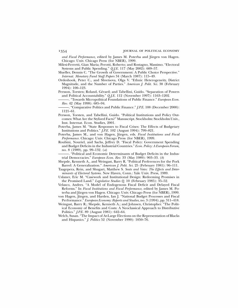
1354 journal of political economy
and Fiscal Performance, edited by James M. Poterba and Jurgen von Hagen.Chicago: Univ. Chicago Press (for NBER), 1999.
Milesi-Ferretti, Gian Maria; Perotti, Roberto; and Rostagno, Massimo. “ElectoralSystems and Public Spending.” Q.J.E. 117 (May 2002): 609–57.
Mueller, Dennis C. “The Growth of Government: A Public Choice Perspective.”Internat. Monetary Fund Staff Papers 34 (March 1987): 115–49.
Ordeshook, Peter C., and Shvetsova, Olga V. “Ethnic Heterogeneity, DistrictMagnitude, and the Number of Parties.” American J. Polit. Sci. 38 (February1994): 100–123.
Persson, Torsten; Roland, Gerard; and Tabellini, Guido. “Separation of Powersand Political Accountability.” Q.J.E. 112 (November 1997): 1163–1202.
———. “Towards Micropolitical Foundations of Public Finance.” European Econ.Rev. 42 (May 1998): 685–94.
———. “Comparative Politics and Public Finance.” J.P.E. 108 (December 2000):1121–61.
Persson, Torsten, and Tabellini, Guido. “Political Institutions and Policy Out-comes: What Are the Stylized Facts?” Manuscript. Stockholm: Stockholm Univ.,Inst. Internat. Econ. Studies, 2001.
Poterba, James M. “State Responses to Fiscal Crises: The Effects of BudgetaryInstitutions and Politics.” J.P.E. 102 (August 1994): 799–821.
Poterba, James M., and von Hagen, Jurgen, eds. Fiscal Institutions and FiscalPerformance. Chicago: Univ. Chicago Press (for NBER), 1999.
Roubini, Nouriel, and Sachs, Jeffrey D. “Fiscal Policy: Government Spendingand Budget Deficits in the Industrial Countries.” Econ. Policy: A European Forum,no. 8 (1989), pp. 99–132. (a)
———. “Political and Economic Determinants of Budget Deficits in the Indus-trial Democracies.” European Econ. Rev. 33 (May 1989): 903–33. (b)
Shepsle, Kenneth A., and Weingast, Barry R. “Political Preferences for the PorkBarrel: A Generalization.” American J. Polit. Sci. 25 (February 1981): 96–111.
Taagepera, Rein, and Shugart, Matthew S. Seats and Votes: The Effects and Deter-minants of Electoral Systems. New Haven, Conn.: Yale Univ. Press, 1989.
Uslaner, Eric M. “Casework and Institutional Design: Redeeming Promises inthe Promised Land.” Legislative Studies Q. 10 (February 1985): 35–52.
Velasco, Andres. “A Model of Endogenous Fiscal Deficit and Delayed FiscalReforms.” In Fiscal Institutions and Fiscal Performance, edited by James M. Po-terba and Jurgen von Hagen. Chicago: Univ. Chicago Press (for NBER), 1999.
von Hagen, Jurgen, and Harden, Ian J. “National Budget Processes and FiscalPerformance.” European Economy: Reports and Studies, no. 3 (1994), pp. 311–418.
Weingast, Barry R.; Shepsle, Kenneth A.; and Johnsen, Christopher. “The Polit-ical Economy of Benefits and Costs: A Neoclassical Approach to DistributivePolitics.” J.P.E. 89 (August 1981): 642–64.
Welch, Susan. “The Impact of At-Large Elections on the Representation of Blacksand Hispanics.” J. Politics 52 (November 1990): 1050–76.