I I

AD/A-002 426

RATIONALE OF COMPUTER-ADMINISTERED

ADMISSIBLE PROBABILITY MEASUREMENT

Emir H. Shuford, Jr., et al

RAND Corporation

Prepared for:

Defense Advanced Research Projects Agency

July 1974

DISTRIBUTED BY:

RAWlu TecWWhnical emi ServieU. S. DEPARTMENT OF COMMERCE

..........

D ...........

SECURITY CL AS AIFICATION OF THIS PAGE (When Data Frntted) _

REPORT DOCUMENTATION PAGE FRED OMSTRUCTIORS1. REPORT NUMBER 2. GOVT ACCESSION NO. 3. FECIPIENT'S CATALOG NUMBERR-1371-ARPA1. .. __

4. TITLE (and Subtt•tle S. TYP"6"1'Rz0;fftnIO COVERED

Rationale of Computer-Administered Admissible IrterimProbabil1itty Measurement P4. PERFORMING ORG. REPORT NUMBER

7. AUTHOR(&) S. CONTRACT ON GRANT NUMBER(s)

".H. Shuford, Jr., and T. A. Brown DAHC15 73 C 0181

S. PERFORMING ORGANIZATION NAME AND ADORESS 10. PROGRAM ELEMENT. PROJECT. TASKThe Rand Corporation AREA & WORK UNIT NUMBERS

1700 Main StreetSanta Monica, Ca. 90406

II. CONTROLLING OFFICE NAME AND ADDRESS 12. REPORT DATE

Defense Advanced Research Projects Agency 3 Jul 1974Department of Defense NUMBEROF PAGESA vI"1 nnt-nn A hc999i p a

14. AMONITONG A C ADDRESS(fit dilfteari Irom Controlliri Olffce) IS. SECURITY CLAiS. (ol thie repon)

UNCLASSIFIEDIla. DECL ASSI FI CATION.'DOWN GRADING

SCHEDULE

IS. DISTRIBUTION STATEMENT (of this Raport)

Approved for public release; distribution unlimited

17. DISTRIBUTION STATEMENT (of the absttact entered In Block 20, If differmnt itom Ropo#i)

No restrictions

II. SUPPLEMENTARY NOTES

1I. KEY WORDS (Continue on reverse side If necessary and identify by block numbot)

Admissible Probability Measurement Computer-Aided TestingTesting Decision TheoryProbability

20. ABSTRACT (Continue on reverse aide If neceacary and identify by block fumbet)

see reverse side

i"n"dg.ed byNATIONAL TECHNICALINFORMATION SERVICE

US C0*m.ent of CemmreeS.10-9Wd. VA. 22151

DD •AN 1473 EDITION OF I NOV 61 IS OBSOLETE UNCLASSIFIEDSSECURITY CLASSIFICATION OF THIS PAGE

1JNCLASSIFl-ED -

S11CURITY CLASSIFICATION Of THIS PAGO(WRM Data X•101")

.4 I

Part of an ongoing study of decision-theoreticpsychometrics. Measurement of a student's know-ledge about the subject matter of a multiple-choice question can be much finer if his estimateis elicited, for each possible response, of theprobability that it is the correct one. Thereport describes the rationale underlying a pro-

• cedure for eliciting such estimates using a pro-"per scoring rule, and new techniques for calibrat-ing those probabilities. The procedure couldyield two classes of benefits: students could

* ilearn to use the language of numerical probabil-ity to communicate uncertainty, and the learningof other subjects could be facilitated. Thereport also presents new results comparing theincentive for study, rehearsal, and practiceprovided by the proper scoring rule with thatprovided by the simple choice procedure, and

concerning the potential effect of cutoffscores and prizes on student behavior.(See also R-1258.) Y. pp. (WH)

*i

SEUIYCAS0I/ UNCLASSIFIED•" ~~SECURITY CLASSIFICATION OF THIS PAGEftian Vm&t Enw.,*

ARPA ORDER NO.: 19-1 I3D20 Human Resources

V

R-1 371 -ARPA

July 1974

Rational .f Computer-AdministeredAdmissible Probability Measurement

Emir H. Shuford, Jr. and Thomas A. Brown

S.,• . --, • ,

ivi

A Report prepared for

DEFENSE ADVANCED RESEARCH PROJECTS AGENCY

AMROVED FOR FUILIC RUEASE; DISTRIIUTION UNLIMITED

-iii-

PREFACE

This report was prepared as part of Rand's DoD Training and Man-

power Management Program, sponsored by the Human Resources Research

Office of the Defense Advanced Research Projects Agency (ARPA). With

manpower issues assuming an even greater importance in defense plaa-

ning and budgeting, it is the purpose of this research program to de-

velop broad strategies and specific solutions for dealing with present

and future military manpower problems. This includes the development

of new research methodologies for examining broad classes of manpower

[ problems, as well as specific problem-oriented research. In addition

to providing analysis of current and future manpower issues, it is

hoped that this research program will contribute to a better general

understanding of the manpover problems confronting the Department of

Defense.

We believe decision-theoretic psychometrics holds considerable

promise for military selection, training, and other applications. In

the past, use of this technique has been hampered by the need to orient

people to a new way of answering questions, and the need to process

the much greater amount of information the method yields.

Because computers now offer a reasonable and, in many cases, a

cost-attractive solution to these problems, we have devised programs

and procedu',es for the on-line administration of tests according to

the requirements of decision-theoretic psychometrics. At this time,

these programs are running on certain IBM 360/370 computer systems

with graphic capability, on the IMLAC PDS-l "smart terminal" computer,

and on the PLATO TV system.

This report provides the rationale for these applications, and

thus should be of interest to potential users and adapters of these

programs, as well as to educators interested in examining in depth

the implications of this new methodology.

4.

I•

$

'• I .... ..i ....... .. --• I ....... " i ... .i , • .. .. . 11... . ....... '| '•r[• '1 ... ... ! ... ... ... ..........i n '' ...... ii ...... ' .......... ...! '' .. ...... ..... " . .. ......

SUMMARY

A student's choice of an answer to a test question is a coarse

measure of his knowledge about the subject matter of the question.

Much finer measurement might be achie-red if the student were asked to

estimate, for each possible answer, the probability that it is the

correct one. Such a procedure could yield two classes of benefits:

(a) students could learn the language of numerical probability and use

it to communicate uncertainty, and (b) the learning of other subjects

could be facilitated.

This report describes the rationale underlying a procedure for

eliciting personal estimates of probabilities utilizing a proper scor-

ing rule, and illustrates some new techniques for calibrating thoseprobabilities and providing better feedback to students learning to

assess uncertainty. In addition, ne-. results are presented comparing

the incentive for study, rehearsal, ind practice provided by the proper

scoring rule with that provided by the simple choice procedure, and

concerning the potential effect of cutoff scores and prizes upon stu-

dent behavior.

A companion report describes an interactive computer program in-

corporating these procedures. See W. L. Sibley, A Piototype Computer

Program for Tnteractive Computer Administered AdvissibZe ProbabiZity

Measurement, R-1258-ARPA, April 1974.

P P

S~PRECEDING PAGE BLANK

-.vii-

PREFACE ................................................... i

SUIM ARY .................................................... v

Section1. ELICITATION OF PERSONAL PROBABILITIES IN EDUCATION .

2. THE CONTEXT OF TESTING ...................................... 3

3. IKOWLEDGE AS A PROBABILITY DISTRIBUTION .................... 3

4. THE EFFECT OF LIMITING RESPONSE OPTIONS .................... 5

5. STRATEGIES FOR RESPONDING TO A TEST ITEM .............. 85.1 Simple Choice Testing ............................... 85.2 Confidence Testing ................................ 105.3 Admissible Probability Measurement ........... 15

6. MARSHALING FACTS AND REASONS BEFORE RESPONDING ...... 20

7. DETECTING BIAS IN THE ASSIGNMENT OF PROBABILITIES ... 23

8. PERCEIVED VERSUS ACTUAL INFORMATION ...................... 29

9. THE CONSEQUENCES OF BIASED PROBABILITIES ................. 37

10. A LIKELIHOOD RATIO MEASURE OF PERSPICACITY .......... 38

11. POTENTIAL IMPACT OF TESTING METHOD UPONSTUDY BEHAVIOR ................................. 42

11.1 Allocation of Study Effort Among Topics 4311.2 Investment of Study Effort in a

Single Topic ................................ 46

12. IMPACT OF INAPPROPRIATE REWARDS UPON TEST-TAKING BEHAVIOR ................................ 47

13. SUMMARY AND CONCLUSIONS ............................. 53

AppendixA. FITTING A PLANAR REALISM FUNCTION ................... 55 I?. HOW TO CALCULATE THE VALUE OF"p" AT WHICH MAXIMUM

EXPECTED RETURN PER UNIT EFFORT IS ACHIEVED ....... 61C. ALLOCATING STUDY EFFORT TO MAXIMIZE PROFIT .......... 66D. SOME RESULTS OF OPTIMAL STRATEGIES TO ACHIEVE

A PASSING GRADE ......................................... 71

REFIM, ZCES ................................................ 75

PRECEDING PAGE BLANK

RATIONALE OF COMPUTIR-ADMINkISTMERD ADMISSIBLE

PROBABILITY MEASUREMENT

1. ELICITATION OF PERSONAL PROBABILITIES IN EDUCATION

Along with the recent growth of the theory and application of the

mathematics of decisionmaking has come an increased interest in expres-

sing uncertainty in terms of personal probabilities. Most of the atten-

tion in this area has been focused upon eliciting personal probabilities

from decisionmakers and experts to guide policy decisions [1-3]. How-

ever, at the end of his comprehensive and excellent review of this area,

Savage [3] refers to potential educational applications of these tech-

niques and states:

Proper scoring rules hold forth promise as more sophisti-"cated ways of administering multiple-choice tests in certaineducational situations. The student is invited not merelyto choose one [answer] (or possibly none) but to show insome way how his opinion is distributed over the [answers],subject to a proper scoring rule or a rough facsimile thereof.

Though requiring more student time per item, these methodsshould result in more discrimination per item than ordinarymultiple-choice tests, with a possible net gain. Also, theyseem to open a wealth of opportunities for the educationalexperimenter.

Above all, the educational advantage of training people--possibly beginning in early childhood--to assay the strengthsof their own opinions and to meet risk with judgment seemsinestimable. The usual tests and the language habits of ourculture tend to promote confusion between certainty and be-lief. They encourage both the v4 ce of acting and speakingas though we were certain when we are only fairly sure andthat of acting and speaking as though the opinions we do

have were worthless when they are not very strong.

Effects of nonlinearity in educational testingt deserve somethought, but presumably nonlinearity is not a severe threatwhen a test consists of a large number of items. One sourceof nonlinearity that has been pointed out to me is this A

Described and discussed in Sec. 5.3.

'Those effects are discussed in Sec. 12.

?I

-2-

student competing with others for a single prize is motivatedto respond so as to maximize the probability that his scorewill be the highest of all. This need not be consistent withmaximizing his expected score, and presumably situationscould be devised in which the difference would be important.

This brief statement characterizes both the promises and the problems

of eliciting personal probabilities from students. The promises come

from two educational goals that might be served by this application:

1. As .i subject matter and skill that is valued in and of itself.For example, it is important for students to learn to dis-

criminate degrees of uncertainty and to be able to communi-

cate uncertainty using the language of numerical probability.

2. As a means of facilitating the learning of other subject

matter, e.g., by providing more information about a student's

state of knowledge.

The problems reside largely in tu areas:

1. Students must be taught a new way of answering questions and

they must overcome bad habits and inappropriate sets induced

by their prior test-taking experience.

2. Great care must be exercised in insuring that the incentive

structure impacting on the student does in fact correspond

to that assumed in the decision-theoretic derivation of the

method, i.e., the student must be motivated to attempt to

maximize his expected score, rather than maximize the proba-

bility of exceeding some standard or surpassing his class-

mates. This ig a subtle point we discuss at greater length

in Sec. 12 below.

The purpose of this report is to describe the rationale underly-

ing a procedure for eliciting personal estimates of probabilit.is util-

izing a proper scoring rule, and to illustrate some new techniques for

calibrating personul probabilities and providing better feedback to

-3-

students learning to assess uncertainty. In addition, new results are

presented comparing the incentive for study, rehearsal, and practice

provided by the proper scoring rule with that provided by the simple

choice procedure, and concerning the potential effect of cutoff scores

upon student behavior.

A companion report [41 describes an experimental version of an

interactive computer program incorporating these procedures and focuses

upon the first problem mentioned above.

2. THE CONTEXT OF TESTING

Students are asked a series of questions to ascertain their know-

ledge of the subject matter represented by the questions. A test item

is composed of a question and a list of k (k - 2, 3, ... ) possible

answers, one and only one of which is correct. A "test" is composed

of n of these items, usually answered in sequence, and where n typi-

cally has a value between 10 and 100.

3. KNOWLEDGE AS A PROBABILITY DISTRIBUTION

While a person holding the answer key is not at all uncertain

about which answer to a question is designated "correct," a student

may encounter a certain amount of uncertainty. In information-

theoretic terms [5], that amount is

ki P10S2 Pi.- ~i-I

where piis tche likelihood (according to the student's view of the

situation) of the event, "Answer i is the correct answer." Because

the pi's may be viewed as probabilities of mutually exclusive and

collectively exhaustive events, we have

0p gPl • I and I pl .Jui=1

i•

-4-

The uncertainty measure, called "entropy" by information theorists,

achieves its maximum value (log 2 k) when all the pi's are equal and

achieves its min1mum val-,' (zero) whet, one pi is unity and the rest

are zero.

There may be several sources of this uncertainty. Some examples

are: the student may not be familiar with the standards and values of

the writer of the test item; the student may not comprehend all of the

language used in the test item; most important, he may not know enough

facts and reasons to arrive unequivocally at the correct answer.

The uncertainty measure itself is unsatisfactory as a measure of

useful knowledge, because it is symetric or nondirectional with re-

spect to the answers. According to this measure, a student would have

minimal uncertainty (and maxi-al information) whenever one of the pi's

equals one. A student holding a probability of one for an inorrect

answer possesses just as much information (in his own view) as does

another student holding a probability of one for the correct answer.

Uncertainty can serve as a measure of learning, but education and

training is concerned with what is learned and must focus •on the prob-

ability associated with the correct answer. Before a student is ex-

posed to a subject matter and tries to learn it, he might be expected

to be uncertain about answers to questions. If a question has three

answers, the student's probability associated with the correct answer

might fluctuate over time but remain close to the value of 1/3 corre-

sponding to maximal uncertainty, as shown by the first segment of the

curve in Fig. 1.

When the student begins to take an active interest in learning the

subject matter, the probability might be expected to rise and bn.gf to

approach one as the student achieves greater and greater mastery of thesubject matter. The student's probability associated with the correctanswer when measured over time might trace a path similar to the learn-

inS curve shown in Fig. 1. Upon completion of the learning phase and

if the student's knowledge or skill is not reinforced, the probability

might begin to decline toward 1/3 and trace a forgetting curve such as

that shown in Fig. 1.

1-5- 1~1.0

i.

PC II.33 II I

I ILearning I Forgetting

0 I

Time

Fig. I -Hypothetical trace of probability oveO time

While these hypothetical curves resemble those found in the psy-

chology of learning, it should be remembered that much of the experi-mental data in this area are reported in terms of averages over either

subjects, trials, or both. Such indirect measures must be used becauseof the discrete nature of the responses made available to the subjects.

If it were possible to take direct and repeated measurements of a sub-

ject's personal probabilities, the need for aggregation of data would

be greatly reduced and the results of experiments might appear quite

different.

4. THE EFFECT OF LIMITING RESPONSE OPTIONSIn the true-false and multiple-choice methods of test administra-

tion, a student is required to select one and only one of the answers

* •The major exception, response latency, is a measure continuous inthe time dimension. Even so, it is frequently averaged because of its

*: instability and, while possibly zeflecting uncertainty, it fpils to con-vey the directional information contained in the distribution of per-sonal probabilities.

-6-

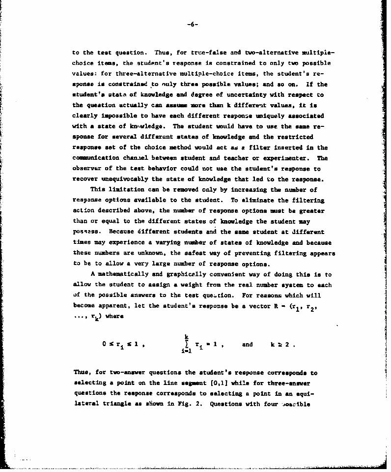
to the test question. Thus, for true-false and two-alternative multiple-

choice items, the student's response is constrained to only two possible

values: for three-alternative multiple-choice items, the student's re-

sponse is constrained to nnly three possible values; and so on. If the

student's stata of knowledge and degree of uncertainty with respect to

the question actually can assume more than k different values, it is

clearly impossible to have each different response uniquely associated

with a state of knomledge. The student would have to use the same re-

sponse for several different states of knowledge and the restricted

response set of the choice method would act as a filter inserted in the

comunication chanael between student and teacher or experimenter. The

observer of the test behavior could not use the student's response to

recover unequivocably the state of knowledge that led to the response.

This limitation can be removed only by increasing the number ofresponse options available to the student. To eliminate the filtering

act-'on described above, the number of response options must be greaterthan or equal to the different states of knowledge the student mayposqass. Because different students and the same student at differenttimes may experience a varying number of states of knowledge and because

these numbers are unknown, the safest way of preventing filtering appears

to be to allow a very large number of response options.

A mathematically and graphically convenient way of doing this is toallow the student to assign a weight from the real number system to each

of the possible answers to the test queý.cion. For reasons which will

become apparent, let the student's response be a vector R - (r 1 , r 2,

rk) where

k

0 :C r 1, 1 r i , and k 2.i-l

Thus, for two-answer questions the student's response corresponds to

selecting a point on the line segment [0,1] while for three-answerquestions the response corresponds to selecting a point in an equi-

lateral triangle as shown in Fig. 2. Questions with four -osxible

-7- 1

Answer

fiir3 -3

! r2 .2

r! .5

Answer Answer2 3

Fig.2 -The equilateral response tricngle used for computer assistedadmissible probability measurement

-8-

answers require three dimensions for a unitary response while questions

with even more possible answers require complex sequential allocation

responses.

5. STRATOCIES FOR RESPOR~fIG TO A TEST ITEM

Merely allowing a student more response options does not insure

that more information about his states of knowledge will actually be

transmitted. The student might, for example, exercise only a minimal

number of the options or, for another example, the way he associates

the response option with his probabilities might be inconsistent or

arbitrary. In either event, the amount of information actually trans-

mitted my be greatly reduced.

A student's state of knowledge, i.e., the facts recalled, reason-

ing, and other thought processes leading to a probability distribution

over the possible answers, are directly observable only by the student

himself. The student's responses are, of course, directly observable

by others, but there is no biological law that a student's responses

must reflect his probabilities. It is, in other words, a matter of

free will and volition on the part of the student as to how he asso-

ciates his response with his probabilities.

In a situation such as this, the best that can be done is to struc-

ture the task given the student so that he is rewarded for consistently

and accurately associating response with his probabilities. Although

the association is one-to-many, this is implicitly done with the simple

choice method of responding used in the administration of achievement,

aptitude, and ability tests.

5.1 Simple Choice Testins

To see this, suppose a student wishes to maximize his expected test

score. With the most frequently used simple choice scoring system, he

earns one point for each correct answer selected and no points for an

incorrect answer. Because his test score is simply the sun of his item

It can be assumed without lose of generality that the student re-ceives no points if he omits an item. Thus, the loss of a fraction ofa point as Illustrated by use of the "correction for guessing" formula

-9-

scores, his expected test score can be maximized by maximizing the

expectation for each item score. Thus, for any item on the test, the

decision problem faced by the student is as shown in Table 1; and his

optimal strategy is to choose that course of action or response asso-

ciated with the maximum expected score as defined by the information

available to him at the time of making the decision. This information

should be reflected in the personal probability distributions as de-fined in Sec. 3.

Table 1

DECISION PROBLEM FACED BY STUDENT ANSWERING ITEMUtIDER SIMPLE CHOICE METHOD

(a Probability5 (That Answer May Be Correct)

Pl P2 " " " Pk

Correct Answer Expected

Response 1 2 . . . k Score

Choose answer 1 1 0 . . . 0 pl

Choose answer 2 0 1 . . 0 P2

Choose answer k 0 0 ."P

It should be remembered that the probabilities characterize the

student--not the item question and answers. One answer is correct--

the others are incorrect. Two different students, or the same student

at different times, may very well possess different probability dis-

tributions over the answers to the same question. The probabilities

reflect the information available to the student at the time he must

make his decision, and provide his only guide to action.

does not change the structure of the task. The structure is changed,however, if the penalty for selecting a wrong answer is greater thank - 1, where k is the number of possible answers to the test question.

-10-

For a student who wishes to score well on a simple choice test,

the optimal test-taking decision rule is, for each item, to select

that answer he considers most likely to be correct. If two or more

answers are tied for maximum probability, it makes no difference which

he selects, because the expected score is the same. This decision rule

may be displayed graphically for two and three possible answers as

shown in Fig. 3.

This analysis makes it apparent that while the simple choice pro-

cedure can motivate a student to use a consistent and logical mapping

of probabilities onto responses, each response represents a very broad

range of probabilities. When a student chooses an answer, all that

may be inferred from this response is that he views no other answer

as being more likely to be correct.

Terms such as "•ell informed," "misinfnrmed," and "uninformed"

are sometimes used to describe a person's knowledge with respect to

some subject. These and related terms can be used to characterize

regions of the personal probability space, as illustrated by the de-

composition shown in Fig. 4 for three possible answers. Because each

point on the triangle corresponds to a possible probability Jistribu-

tion over the three answers, this classification 3roups distributions

that may have a similar import. For example, if a student had no

reason for very strongly preferring any answer over the others, his

probability distribution would be located near the center of the tri-

angle and he would be "uninformed" with respect to the item. Figures

3 and 4 may be compared to see what information is yielded by the

response-to-probability mapping induced by the simple choice method.

The relations can be summarized as in Table 2.

While the simple choice response is clearly intapable of discrim-

inating many states of knowledge, a free response such as that described

in Sec. 4 would have the potential of transmitting a great deal more

information about a student's state of knowledge. Will this informa-

tion actually be transmitted?

5.2 Confidence Testing

Suppose, as before, that the student wishes to maximize his ex-

pected test score and that he is allowed to distribute 100 points over

-11-

Two possible answers

Choose ChooseAnswer 2 Answer I

Answer 2 Answer I

Probability line

Three possible answers

Answer 1

Choose Choose

Answer 2 Answer 3

Answer 2 Answer 3

Probability triangle

Fig. 3- Optimal decision rules for two and three answers

S~I

...

-12-

Correctanswer

"Well informed"

"Informed"

Uninformed"

"Misintormed""Bc..dly • 'Badly .

misinformed " . .risi nformed

Incorrectans•wer answer

Fig.4-One possible decomposition of the probability triangleto represent some meaningful categories of knowledge

-13-

Table 2

IFEUNn ES THAT MAY BE DRAWN FROM THE SIEMLE CHOICE RESPONSE

If the studenthas selected Student may be: Student is not:

Well informed MisinformedInformed Badly informed

The correct answer Partially informedUninformed

Partially informed InformedUninformed Well informed

An incorrect Ser MisinformedBadly informedIf

the possible answers to each item as is sometimes done in "confidence

testing." This would provide a met of responses fine-grained enough

to transmit considerably more information and it would be quite simpleto score the student according to the number of points he allocated to

the correct answer. To be more explicit, let a1 1 be the number of

points allocated on the Jth item to the ith answer, where

kO9mij 1100 and m 100 iI

Let the test score be

Sre, =j,

where ms is the number of points allocated to the correct answer to

"item J.

The potential impact of this scoring rule upon student behaviormay be investigated by finding, as before, the optimal test-taking

strategy for a student who wishes to maximize his expected test score.Because his test score Is simply the sum of his item scores, his ex-

pected test score can be maximized by maximiping the expected score )

-14-

for each item. There are now far too many response options to list in

a table, but the expected score for any allocation on a single question

(mi, t2, ...2 m.k) may be written as

B(ml a 2, "" uktl1 P2 ' ..." Pk)"lP + a2 P2 + "'" + mkPk

It is not too difficult to find the optimal decision rule, i.e., to

specify for each probability distribution that response (allocation of

points) which maximizes the expected item score. Because the labeling

of the answers is, In a sense, arbitrary, we may assume without loss

of generality that

p1 l p2 • p3 e ... Pk

i.e., the answers can be reordered from most likely to least likely to t

be correct in the view of the student. The decision problem is one of

allocating points so as to maximize the sum of products as shown below.

mlp 1 +2P2 + ... + mkPr

The points may be placed one at a time because the placing of a point

does not change the structure of the problem. Allocating a point to

answer i yields a return of pi because only that proportion pi of the

point will be added to the sum. If P1 > P2' then the first point should

be placed in the first position in order to yield the largest possible

return, p,; the second point should also be placed in the first posi-

tion: and so on for all 100 points. If P1 - P2' or if p1 = P2 = P31

and so on, the points can be distributed between these maximum proba-

bilities, but there is nothing to be gained by so doing. The optimal

test-taking strategy for this scoring rule can be sumarized as, "Find

an answer that is at least as likely to be correct as any other and

allocate all 1.00 points to this answer."

Thus, this scoring rule induces a mapping of response onto proba-

bility that degenerates into the simple choice situation (see Fig. 3).

-15-

Although many response options are offered to the student, he is max-

imally rewarded for placing all 100 points on the most likely answer.

If a student follows this best test-taking strategy, his responses will

be essentially indistinguishable from choice type responses and no

additional information will be transmitted about his states of knowl-

edge. This example shows that merely offering an increased number of

response options does not guarantee that more information will be

transmitted.

5.3 Admissible Probability Measurement

What is required is a scoring rule that can motivate the student

to use more of the response options, each associated with a small region

of probabilities. In the limit, this relation could be expressed as

ri = f(pi), where f is a monotone increasing function of p and all of

the potentially available information could be transmitted. There are

other cogent reasons, however, for further constraining f to be the

identity function, i.e., r1 " Pi-.

With the identity relation, the student's responses are directlv

interpretable as probabilities and these numerical quantities can be

used in the equations of probability, information, and decision theory

[1]. Students would be learning to communicate degrees of uncertainty

in a universal language of probabilities. For this reason and in the

absence of any compelling reasons to do otherwise, it seems reasonable

to require that scoring rules possess the property that a student can

maximize his expected score if and only if his responses match his

probabilities. Scoring rules satisfying this condition have variously

been called "proper" [3], "reproducing" [1,6], and "admissible" [6).

It has been shown that there exist an infinite number of scoring

rules that induce the identity relation between response and proba-

bility [1,61. Only one, however, possesses the property that the

score depends only upon the response assigned to the correct answer,

and not upon how the responses are distributed over the other answers

when more than two answers are possible [6]. This is the logarithmic

scoring rule, which -my be written as Si A log ri + B, where A > 0.

Vi

-16-

Notice that log ri - -• when ri 0 0. This means that the loga-

rithmic scoring rule cannot be strictly applied In practice, because

if a student ever assigned a response of zero to a correct answer the

logarithmic scoring rule calls for an infinite penalty. However, by

restricting the range of possible responses that a student may use,so that r. l d (where d might be set at 0.01 or some other smal value)

the need for a very large penalty is avoided, but with the sacrifice[.*

of some accuracy in measuring very small probabilities [61.

For many purposes it seems desirable to adjust A and B so that

when a student possesses no information with respect to an item (i.e.,

all p's are equal), his score will be zero. This may be accomplished

by choosing a range, K, of possible scores and setting A - 0.5K and

B - 0.5K log k, where, as before, k is the number of possible answers.

The score that the student will receive if answer i is correct can now

be written:

S(ri) = 0.5K log kr1 , ri 2 0.01

A range of 100 points appears satisfactory for oany applications.

Figure 5 shows graphically the conditional scores for the case of two

possible answers while Fig. 6 shows selected conditonal score triplets

for the case of three possible answers. Notice that in the case of two

alternatives, the maximum score obtainable is about 15, while the mini-

mum score is about -85. In the case of three alternatives, the maximum

is about 24 and the minimum is about -76. This difference in maximum

and minimum scores is caused by the requirement that the scoring func-

tion be zero when all the responses are equal, but Lt may also be taken

to indicate that prediction may be, in some sense, easier with two

alternatives than with three.

Notice, also, how the penalties tend to be larger than the rewarr.s.

This is a characteristic of all th.. admissible scoring -iles because

the nonlinearity is required In order to induce matching behavior in

For those special situations requiring the accurate measurementof very small probabilities, d may be set at a very much smaller value.

-17-

15

0

S (r I)

-15

-30 S(r 2 )

-45

-75

0 0.1 0.2 0.3 0.4 0.5 0.6 0,7 0.8 0.9 1.0Respose (r

Fig. 5- Conditional score functions for the case of two possible answers

Becouse r2 I - r1 conditional score pairs may be found where r1 r.

tv~

-18-

ANSWER I

(24, , -6.

(22.-2/-16) (22,-.\7.2.6)

(19.-IU ) ) (lO,-6, -2) (,-YG,-I1)%

( I4 . 4 -7 ) (13 ,-2 , -26 ) (1, - -.11) (1J - 4. -2 ) (1 -IC, 4 .)

(4. 1, -•1) ( 14 -2. 2) (,. 0. -11 - 2) (4 , - 24 , - ( 1• -76, 4)

10 00 0 0"

(-, 1. •-76) (-4, 12, -2.1) (-2,. .- 11) (-2.4,-I•) (-2,-2.4) (-2,-lI, 'e) (-2,-b .- 6, ) (-4 7.*'••

-6, o, I', (- *,-5) (-.., 16, II) (-;5,21.1,. ()6,',41 1-46,4, 11 (46,-.(I ( ,17,-I ) 1 -4,-*6, 1.) (. 26, V- x , 22)

7 1,74.. 6 -76 , ') (-T, h1, 110) (It', 16.) It, 11.,4) (7•*1 16 ,) , 4, 1I) ( *6. -1, IC) •2. I ,-I1,6Il) (.- 76. '1,, 1) (-16. -76, 24)

ANSWER 2 ANSWER 3

Fig. 6- Conditional score triplets (based on logarithmic scoring function)for some selected responses on the equilateral probability triangle

-19-

the students. This characteristic of the scoring rule may have other

implications, as illustrated by this quotation f,,om a Rand staff mem-

ber after experiencing computer-assisted admissible probability measure-

ment as reported in (4].

One thought that occurred to me after I took (the) testwas that, contrary to other tests, this one can also bea learnt'aj experience. The situation in which one ispunished severely for emphatically stating what turns outto be wrong, more so than one is rewarded for what isright even if emphatically stated, is one that is closerto the reality situation of everyday life than the simpletests that look only for right or wrong. Thus, the testitself exercises a certain negative reinforcement againststating too strongly what one is not really sure about,and thus actually conditions a person to using what knowl-edge he has, and at the varying degree of rertainty withwhich he commands it, judicioeZzy. This will be of ad-vantage to him in life. For it is a fact of life that amistake stated with aplomb permanently reduces our credi-bility with others who must rely on our say-so, i.e., itmakes us less likely to succeed in a Job, tor instance.Thus (the) test is not only evaluative but educational.

Consider now the optimal test-taking strategy for a stutdent who wishes

to maximize expected test scores. As beforf, the total test score is

simply the sum of the item scores, so expected test scores can be maxi-

mized by maximizing each expected item score, which may be expressed as

S~ki" E[S(r)IP] S • P1 S(rt)1 i-I

k

kk

p P(0.5K log kr )

kO.5K(log k + , pi log ri)

i-.

-20-

This last form of the equation makes clear a relation between the

logarithmic scoring rule and information theory. If a student responds

with r- p for all I, then his expected item score is proportional to

a constant plus the amount of information he perceives that he possesses

with respect to the ithm. This relation mukes it easy to derive Informs-

tim measures from test scores based on the logarithmic scoring rule

(cf. Sec. 8).

Should the student respond with his probabilities or, more speci-

fically, how does the logarithmic scoring rule induce the student to do

this in order to maximize his expected scores? Figure 7 shows, for the

case of two answers, expected scores for all possible responses for each

of the four different probability distributions, while Fig. 8 shows ex-

pected score contours for the case of three answers. Notice that for

each probability distribution the largest expected score occurs where

the response matches the probability distribution. With an admissible

scoring rule such as the logarithmic, this is true not only for these

selacted distributions but for all possible probability distributions.

This means that a student always suffers a loss iu ex-pectcd score when-

ever he deviates from the optimal test-taking strategy of settingrl "p for all 1. Note further that the loss in expected score in-creases the more he deviates from this optimal strategy. For those

instances in which the student has no knowledge about an Itew, i.e.,

all the p's are equal, if he pretends to have complete knowledge by

setting one of the ri a 1, he loses 35 points in expected score when

there are two answers and almost 43 points when thero are three answers.

This feature of the logarithmic scoring rule may be expected to serie

as a disincentive toward guessing-type behavior. More important, how-

ever, the logarithmic scoring rule can serve to indice an exact a!so-

ciation of responses with probabilities. What other impact might It

have upon student behavior?

6. MARSHALING FACTS AND REASONS BEFORE RESPONDING

Up to this point the decision analyses have taken the student's

uncertainty (his probability distriLution) as given, and then focused

on finding that response which gives the highest possible expected

. .-.. 1....

-21-

1.5 1.5AB

0 0

15 -15

~-30 &-30-

I•.-45 -4 5

2-60 0

LU 'LU-75 -75

-90 I i I i i -90 _I_____I_ ________

f 0 0.2 0.4 0.6 0.8 1.0 0 0.2 0.4 0.6 0.8 1.0

Response Response

1.5 1.5

--, 0 ,.-- 0-

"• -15 -15CL C

. -30 30

-45 -45

,. ..-'60 -- 60,

-5 -75

- 9 0 i I , , i i I i- 9 0 -- j• l ; ,

0 0.2 0.4 0.6 0.8 1.0 0 0.2 0.4 0.6 0.8 1.0Response Response

Fig. 7- Expected score functions in the case of two answersfor four selected probability distributions

ISW.24. . . .- k

-22-

4014.1

tSA

S4S. - - - - - - -,

S) . .. 0 -- -

E[S(r) p 1 -1 7 j , P2 3 ELS~r)IP,= /. P2 1/2~.O, P3-/3]

151 /

/ o

Fg 8- Et

/o / s c p

--. 0----./ ./ \

-- -- /< .-.. -____ .o " -= - -- -. ' -- -- "

SFig. 8- Expected score contours in the case of three answersS~For four selected probability distributions

-23-

score. There does conic a time during the taking of any test when the

student has to commit himself to some response. The optimal strategies

derived above are appropriate to this problem and, thus, are designated

teat-taking strategies in the narrow sense.

The scope of the decision context must be enlarged, however, when

it is considered that a student may have some control over his proba-

bility distribution for an item. For one example, while taking a test

he can think more deeply about the questions and answers to bring more

facts and reasons to bear upon the problem at hand. For another ex-

ample, prior to taking a test he can study in order to gain additional

information about the subject matter. What implications does the scor-

Sting rule have for these types of behavior on the part of a student?

;iven that a student uses the optimal response strategy, r , his

optimal expected score. E[S(r )Ip] - k piS(r*), can be computed for

each possible probability distribution. Figure 9 shows this relation

when there are two possible answers for both the simple choice or linear

and the logarithmic scoring rules. Notice that as the student acquires

information to move his probability away from the state of being un-

informed (P0 P2 0.5). the optimal expected score from the simple

choice procedure increases in proportion to the distance moved along

the probability scale, while that from the logarithmic scoring prnce-

dure increases only slightly at first and then more and more as higher

levels of mastery are achieved. A similar effect is observed in the

case of three possible answcrs, as shown in Figs. 10 and 11. Thu.s, the

logarithmic procedure requires a higher level of mastery !o yield any

given optimal expected score (other than zero) than does the simple

choice procedure and, in this sense, can serve as a more striagent in-

centive system for learning. In Sec. 11 we build a model to investigate

this in more detail.

7. DETECTING BIAS IN THE ASSIGNMENT OF PROBABILITIES

The central theme so far has been concerned with the relation be-

tween a student's responses and his probabilities. The probabilities

were taken as given and tl,, relation (if any) between the student's

probabilities and thi, external world was reflVCt, d indirect Iv in thi,

studentts actual test score.

A4

-24-

15

Simple choice or linear

- Logarithmic

12 /\ /\ /\ /

o~0.6

- /

Q.0.3

\I /

0 0 . . . .0.6 0. 0. 0./.

S\ /\ /\ /

\ J/

0.3- /

\\/

0 0.1 0.2 0.3 0.4 0.5 0.6 0.7 0.8 0.9 1.0

Probability

Fig.9-Optimal expected score as a function of probabilityin the case of two answers

tI

-25-

Answer

24

20

*1 Iis

10

5 1

€0

24 24Answer Answer

2 3

Fig. 10-Optimal expected score for simple choice and linearscoring rules in the case of three answers

A

-26-

Answer1

24

15

10

E [S (r") p1, P2 P3 ]

0*

1 0 10

24 24Answer Answer

2 3Fig. 11- -OptimaI expected score for logarithmic sýoring rule

in the case of three answers

-27-

Here, the focus will be on the assessment of probabilities them-

selves, i.e., on the relation between the student's probabilities and

the facts and reasons leading to these probabilities. It should be

recognized that there is a point beyond which this type of analysis

cannot go. There exists no completely general descriptive or prescrip-

tive theory of how to derive probabilities from facts and reasons.

Even if such a theory did exist, there is at present no way of knowing

what facts and reasons a student is aware of at a particular moment in

time. Nevertheless, a number of powerful methods for the assessment

of probabilities are currently available or under development.

The externa 'aliditj ,rraph is the most fundamental means of call-

brating and operatiunally defining personal probabilities. Assume that

a student taking a test is following the optimal test-taking strategy

for the logarithmic scoring rule so that r - p. Now let

N(CIp) = number of correct answers assigned probability p

and

F N(Ilp) = number of incorrect answers assigned probability p

Then

r(p) H(Cp) + N(I'p)

is the empirical success ratio conditional upon the probability assign-

ment p. A student's probability assignments are perfectly valid if

R(p) - p for all p when the number of observations is increased without

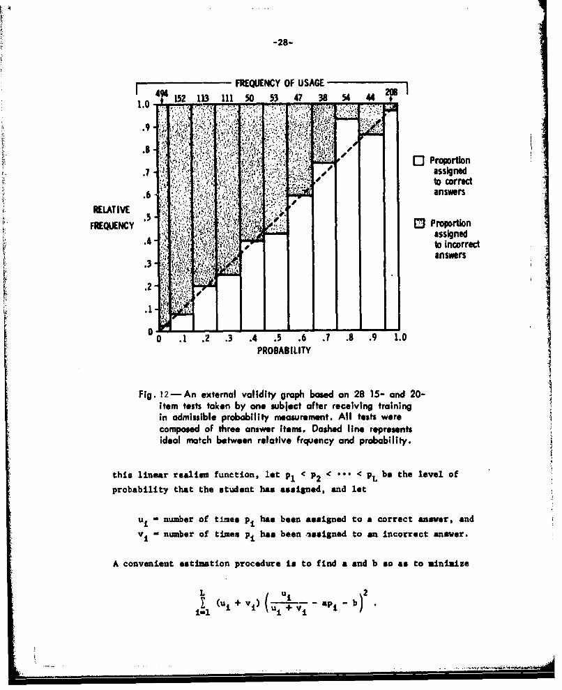
limit. Figure 12 illustrates an external validity graph.

An external validity graph requires an inordinate amount of data

before a student's probabilities can be calibrated. However, by plac-

ing some constraints on the relation between relative frequency andprobability, it is possible to obtain some results with much less data.

Suppose, now, that R(p) tends to q = ap + b, 0 . q • 1. To estimate

-28-

FREQUENCY OF USAGE152 13 111 50 53 47 38 54 44 2

~ -~Prouorion.7 assigned

S# .~ . .~....to correct.6 ... :'7;answers

RELATIVEF.REQUENCY. A~.:1 Proportion

FREQUNCY tX ~assigned

*~ ~ 'to Incorrect.3 J ~ *answers

0 .1 .2 .3 .4 .5 .6 .7 .8 .9 1.0PROBABILITY

Fig. 12-An external validity graph based an 28 15- and 20-item tests taken by *on subject after receiving trainingin admissible probability measurement. All tests werecomposed of three answer items. Dashed line represents4ideal match between relative frquency and probability.

this linear realism function, let P1 < P2 < ** p etelvlo

probability that the student has assigned, and let

Uj . number of times pi has beon assigned to a correct answer, and

vi number of times pi has been assigned to an incorrect answer.

A convenient estimation procedure Is to find a and b so as to ininiaize

L u )2S(ui i)(1- +- v, -a-I b

-29-

The least square estimators are (see [151):

(u+ v1 ) + uv -I.(u + vj)pi Juia ". .u . 2 1 (u. + vi) - [X(ui + vi)pi]2

I + vi )Pi

2 •

-(uI + V(u + vi)P ub m up N p

uI + vi)P• 2(ui + vi) - [1(ui + vi)PI]2

As long as a reasonably wide range of p's is used by the student, this

estimation procedure can yield fairly stable results with 15- and 20-

item tests, so it represents a tremendous improvement in efficiency

over the external validity graph. it should be noted that if the slope

estimate a > 1, the student appears to be undervaluing his subject

matter information, while if a < 1. the student is apparently over-

valuing his information (see Fig. 13). This analysis of bias appears

to be completely satisfactory for the case of just two possible answers

to each test item. Where three or more answers are allowed, however,

this analysis requires that each response/probability is independent of

the others in the distribution. This is not necessarily true for all

persons. For example, some people might tend to overvalue information

when deducing reasons in favor of an answer, but tend to undervalue

information when deducing reasons against an answer. In Appendix A we

* give a planar estimation procedure for the case of three possible

answers. This procedure is capable of detecting the separate dimen-

sions of bias.

The calibration results yielded by the realism function are re-

lated not only to Savage's conjecture quoted at the beginning of this

report but also to a familiar saying of Confucius: "When you know a

thing, to hold that you know it and when you do not know a thing, to

acknowledge that you do not know it. This is knowledge."

8. PERCEIVED VERSUS ACTUAL INFORMATION

This aspect of student behavior may be explored further by com-puting (under the assumption of independence among test items) the

-30-

0 /

0PrbaiI t

Fi.I/ w els ucin bsdo rbblt sinet

to thesubjec matte of th testrosbib i cae lit>pobbiit

assignment; I.e.,

n kn log k+ ~~Pl8 1

If the logarithmic scoring rule is uaed, Lhis expression when multi-

plied by 0.5K becomes the difference between the test score the student

-31-

expects and the test score he would expect if he had no information

relevant to the subject matter.

The amount of information the student actually possesses with re-

spect to the subject matter of the test may be estimated by substitut-

lng - max[O, *in(l, ipij + b)) for the Pij in •he above expression.

Comparison of these two information measures reflects the extent and

direction of student bias. This comparisoi may be made graphically

in terms of the infoontiition equare shown in Fig. 14, which has been

drawn to illustrate the aptness here of the Arabian proverb,

He who knows and knows that he knows,He is wise, follow him.

He who knows and knows not that he knows,He is asleep, awaken him.

He who knows not and knows not that he knows not,

He is a fool, shun him.

He who knows not and knows that he knows not,He is a child, teach him.

Wisen log k n log k

00

o E

00C I E

U U

LC

0 0Child

ric1 . 14 The infomatlon $ sqciare

Under certain conditions, however, the information measures mnybe equal but the realism function reveals that the student is tendingto overvalue his informiation. These instances tund to be uxtreme andeven pathological, e.g., when a nsudent tries to minimize hi.s vxpectedtest score.

-32-

At Rand we have demonstrated, and tried out, computer-administered

decision-theoretic testing with many different people using as sample

tests Reader's Digest vocabulary testa; Humanities, Natural Sciences,

and Social Sciences items from a workbook for the College Level Examin-

ation Program tests; and a midterm postgraduate-level test in Icono-

metrics. About halfway through these demonstrations we decided to begin

keeping a permanent record of what people were doing at the terminal.

Figure 15 compares the two information measures for the first test

taken by each of 66 people. Most of the data points fall below the

diagonal, indicating that most of the "subjects" at least initially

overvalue their knowledge of these subject matter areas. A few people

full close to the diagonal, suggesting that some people may exist who

can discriminate with great accuracy what they know well from what they

know less well.

What happens when people take more tests and, thus, gain more ax-perience with decision-theoretic testing? We find that many people can

reduce their score loss due to lack of realism [41. I think that this

improvement comes as they begin to experience the consequences of the

admissible scoring system [61 and leaxi to reduce their risk-taking

tendencies by making their utilities more nearly linear in points earned

or lost. There does, however, appear to be a limit to this improvement.

A number of people were encouraged or challenged to take more tests,

and to try to be as realistic and to score as well as they possibly could.We ended up with 11 subjects who took an appreciable number of tests--enough so we could discard the early ones they took while they were

learning the procedures and the consequences of the admissible scoring

system.

Figure 16 shows the apparently stable state behavior of the most

biased of the 11 subjects. The line designated YA is located at the

mean of the actual information measures, while the line designated I•

is located at the mean of the perceived information measures. The in-

tersection of the two lines gives a gross indication of actual versus

perceived information for those tests the subject decided to attempt.

By taking the ratio of Ip to I-A we can obtain a rough measure of the

extent and direction of bias. The ratio for this subject is 2.44, in-

dicating that she thought that she had almost two and one-half times

as much information as ahe actually had.

-•.,.-., . ,,.:_- , : .. , •-:•• •.'-- . ..- . ..-- - ;•. . • ,, ,: ,• I .. • • ' • ,," ,u •=,- •, • '• -' " •= " " '-• " " ' : • " • • : ,'f

-33-

00

S S

8 S

•0 Percive

< .A0 T0

C •o° eS • °o

• • %0

"PercPerceivedFig. 156 - Information comparisons for 66 subjects

while taking first somputer- d.dmi nhtered

ad lmiost ble probability test

. .

ii'A

x-

" • •

rC

!' 0""' 0

•. Perceived information•: Fig. 16-- Information comparisons for subject A, theS; ~most biased subject. Early tests excluded. Data shown _

; for last 18 tests taken by subject

-34-

Table 3 lists some personal characteristics for the 11 subjects

arranged in decreasing order of bias, which goes d ,wn almost to the

unbiased value of 1.00. Notice that no subject yielded an overall

ratio less than one, which would have indicated a person who typically

undervalued his information. Figure 17 compares the information meas-

ures for subjects B through K. Subject B, although apparently striv-Ing to reduce bias and to improve his score, waa unable to do so. The

remaining subjects, depicted in decreasing order of bias, were rre and

more often euccessful in producing a realistic assessment of their un-

certainty. Subjects J and K, the two most accurate subjects, were

remarkably consistent in demonstrating their ability to assess their

uncertainties accurately.

Table 3

SUBJECT CHARACTERISTICS

Subject 'P/'A YA Tests Sex Age Education

A 2.44 0.31 18 Woman 20-30 Master's +B 2.42 0.17 12 Man 30-40 DoctorateC 2.26 0.28 7 Man 50-60 DoctorateD 2.11 0.32 27 Woman 20-30 Bachelor 'sE 1.81 0.18 20 Woman 20-30 Some collegeF 1.67 0.40 12 Woman 50-60 DoctorateG 1.52 0.30 20 Woman 30-40 Bachelor'sH 1.33 0.35 9 Girl 9 Third grade1 1.22 0.38 21 Girl 12 Fifth gradeJ 1.02 0.71 34 Man 40-50 DoctorateK 1.00+ 0.85 8 Man 40-50 Doctorate

In cor.clusion, the introduction of decision-theoretic testing makes

it possible to define and to measure for the first time a human ability,call it rea~isrm, which may prove to be a -ý..ry inpurtant determinant of

individual and team performance. For example, to what e:,tent and in

what manner is an unro-alistic student handicapped in his attempts to

learn and to study effectively? For another example, does a team of

realistic people tend to out-perform a team of overvaluing people and,

ii so, for what types of tasks? Answers to these and many other ques-

tions must await further research.

B6 C

C

0 1

D0

.20

A

/ 000

°I eqZ

'A

IP 0

0. 10 c

D /

ai -

-- I* CtFi.1 0n(rmto coprsnfrsbecsBtruhK0

0]

-36-

H

.2

0

4 K00

C00

0 C

0 0

Fg .1

theirve I nformation. WedPo e nwwa eficived Info thisniit

exist within different subgroups of the population nor do we know

exactly how to go about educating people to become note realistic. The

results for subject A, suimiai'ized in Pig. 16, certainly prove that

level of education does not i.noure realism in assessing and comimnicat-

Ing uncertainty.

-37-

9 THE CONSEQENCES OF BIASED 0PROBABILITIES

Decomposing the test score provides a convenient means for shovIng

a student the consequences of having less than perfect realism inassessing the value of information. It is also related to a majoz, butlittle known, property of an admissible scoring system: A student's

actuaZ test score is marimi•ed if and onZy if his responses match theconditionaZ success ratios defined in the previous seotion. Thus, the

effect of experience upon a student who desires to score well on admis-sible probability tests should be in the direction of making his re-

sponses conform more closely to the conditional success ratios. Inother words, the student should develop his ability to give better

probabilistic predictions.

The maxim- test score obtainable on an n-item test with the logs-ritbuic scnring rule is M(n) - n(O.5K log k), while the minimm score

is m(n) - n(0.SK log 0.01K) because of the restriction on r. If S(n)is the total test score earned by a student, then M(n) - S(n) is the

amount of Improvement left in order to achieve perfect mastery of thetest, and when K - 100 this total Improvenent score can range between0 and lOOn. Thus, one function served by the use of an improvement

score is the elimination of negative scores.This total improvement score may now be broken down Into two scores,

each of which has a meaningful interpretation. Suppose the test is re-scored using the adjusted probabilities ptj, computed from the student's

realism function as described above, instead of the student's actualresponses rij. This procedure yields a new score, S(n), which typicallyis greater than or equal to S(n).t The adjusted score S(n) is an asti-mate of the score the student could have made if he were unbiased and

For a student who it biased in assessing uncertainty, i.e.,p 0 r(p), we have the possibility of conflict between maximizing ex-pected score versus maximizing actual test score. While of profoundimportance, a detailed treatment of this subject is beyond the ucopeof this retort. The conflict is resolved, of course, if the studentis able to change his probabilities to match the conditional su-cessratios.

Recall that the realism function is only a least-squares fit tothe data. If the realism function were fitted using a maxinum like-lihood procedure,'the logarithmic scoreyvould be strictly maximizedand there would be more assurance that S(n) k S(n).

-38-

made more effective use of the information available to him. Now,

S(n) - S(n) represents the improvement possible through more effective

use by the student of the information already available to him, while

M4(n) - S(n) represents the improvemsent possible as a result of his gain-

ing additional information pertaining to the subject matter of the test.

These two improvement scores are a decomposition of the total test score

because, when sumed, they equal the total improvement score. Such an

analysis, of course, is not possible with the simple choice method.

10. A LIKELIHOOD RATIO NEASURE OF PERSPICACITY

Realism appears to be an important. goal for human behavior. Thereis some indication, however, that it may not be sufficient as an ideal.

For example, by using complex strategies which sacrifice potential test

score, a student might be able to produce a realism function with a

slope nearer to one. This kind of pseudorealim must not be produced

at the expense of test score and if the proper emphasis is placed upon

score, it probably will not be.

For another example, there is the question of a student's ability

to discriminate levels and patterns of uncertainty. To illustrate,

consider some data from a 15-item, three-answer test. Figure 18 shows

the 15 probability distributions elicited from a student inexperienced

in explicitly assessing uncertainty. It appears that this student was

thinking in terms of which answer was most likely to be correct and, as

a result, responded along the line going from the no-information point

up to complete information. Figure 19 shows the 15 probability distribu-

tions elicited from a student with considerably more experience in ex-

plicitly assessing uncertainty. it appears that this student would

sometimes use information to "rule out" one of the answers and perform

other kinds of complex discriminations yielding a variety of probability

distributions.

Consider now using just one probability distribution to represent

each student's knowledge. Let p' be the highest probability assignedj

for item J, p" be the next highest, and p"j' the smallest. The average

probability distribution (p, p', P1) may be found by calculating

S.

-39-

0

Iii

Fig. 18 Probability distributions (ignoring permutations amongthe answer labels ) used by inexperienced subject taking one

15-item test and yielding a likelihood ratio of .214. Circlerepresents average probability distribution.

[ !

-40-

0

Fig. 19-- Probability distributions (ignoring permutations amcongthe answer labels ) used by highly trained subject taking one15-item test and yielding a likelihood ratio of 36.55. Circle

represents average probability distribution.

4- d J '.

n I J1 a and - •i-i i-i -i -

This average probability distributi:on is displayed as a circlo in Figs.

18 and 19. Notice that Lhe. are not strikingly different for the two

students.

Which set of probobtlity distributions, the original set or the

average one used for all items, is the better predictor of the set of

correct answers? To be nore specific, consider the "data" to be the

sequence of correct answers and let pcj be the original probability

assigned by the student to the correct answer to item J. Then, the

likelihood of the data under the hypothesis that they were generatedby the student's probability distributions is

j-l

Now consider the hypothesis that the data were generated by the con-

stant average probability distribution. That is, look at Pcj and give

it the value p', p". or p"' according to whether it was the largest,

middle, or smallest probability in the set. Or, equivalently, let

no - the number of times Pcj was largest,

n" - the number of times pcj was next largest, and

n" the number of times jcj was the mallest, so that

no + not + net$ a, U

If there are ties among the Pcj' fractional numbers must be used. The

likelihood of the data under this second hypothesis can be written as

- - --. ......-.. .--.- .

inP"" ' •oo

!L2

-42-

The likelihood ratio can now be computed as L1 /L 2 . For the data shown

in Fig. 18 this likelihood ratio is about 0.2, indicating that the data

are about five times more likely under the constant probability hypothe-

sis. For the data shown in Fig. 19 this likelihood ratio is about 37,

indicating that the data were about 37 times more likely using the

student's original set of varying probability distributions than using

the constant average probability distribution. Thus, this likelihood

ratio may prove to be a useful measure of a student's progress in learn-

ing how to extract and process information in probabilistic terms.

11. POTENTIAL IMPACT OF TESTING MET•OD UPON STUDY BEHAVIOR

Because lower levels of mastery often require much less effort toachieve than do the higher levels, the logarithmic may prove to be a

very appropriate reward system that can motivate students to achieve

higher levels of mastery of a subject matter than they do at present.

To investigate this, assume that the student has. for each question,

an exponential "learning curve" of the form

1p - 1 - 1 exp (-2Xc)

where c represents the cost to the student in time and energy, say, ofthe effort he puts into studying the question; ) is a parameter thatreflects the "easiness" or rate of learning of the subject matter of

the question; and p is the student's probability associated with the

correct answer. For the sake of definiteness and simplicity, assumethat each question has only two possible answers. Thus, if the student

plii no study at all into the question (i.e., c - 0), his probability

for the correct answer is 0.5, but as he invests effort in studying the

subject matter his probability increases asymptotically toward 1.0, as

illustrated in Fig. 20.

There are two ways of modeling the way a student will choose to

spend his study time and effort. You •.L.ty either assume that he has a

fixed amount of time available and seeks to allocate it across the

questions in s'ich a way as to maximize his optimal expected score; or

-| ,. . . . . . pc4. . . . . . . . . . . . . . .

3.0

0.9 X

>.0.8

0.6

0.50 12 3

5 Effort

Fig,20 - Pobabuity as a function of effort, c, where p 1 - 1/2 exp( -2 X c)

you may assume that there is some "exchange rate" between study timeIand score (e.g., one point of score is worth three minutes of time to

this particular student) and that he will "spend" his time on each ques-

tion in such a way as to maximize his "profit," i.e., the difference

between his optimal expected score on a question and the value of the

* time he expends on studying it. These approaches will be discussed

separate~ly, but It will become apparent their solutions are closely

* related.

11.1 Allocation of Study Effort Among Tcopics

First, suppose thaL- the student has a fixed and limited amount af

study time available and wishes to allocate It over the questions likely

to be asked in such a way that he wilU7 maximize his optimal expected* ucore. On a given question, by following the optimal tes.t-taking sitrat-

* egy he will expect trn score

E[s(r*)Jp(c)1 - *

where p(c) is the function of study time and effort defined in the pre-

vious section. Figure 21 shows optimal expected score as a function of

effort for a single question under both the simple choice or linear and

the logarithmic scoring procedures. The uaximum return (in terum of

expected score) per unit of effort may be found graphically by measur-

ing the slope of the steepest line through the origin which is tangent

to the optimal expected score.function, K . Analytically, it can beEdetermined by finding the point where the derivative of (c) with re-

spect to c is zero. Now in fact,

dE-(I p)log[2(l -p)]Tp- -E,d E I________A_____E

"c •cdp dc 2 2 ' 2c c

Because of the particular form chosen for p(c), it follows that the

numerator of this expression depends on p alone, not on c or X. Thus,

there exists a "critical value" of p, say p , for any given scoring

rule such that on any question and regardless of what X may be, the

student will get maximum reward per unit effort to bring his probability

for the correct answer up to p

It is easy to calculate p for any given scoring rule (see Appen-dix B). To be specific:

SCORING RULE CRITICAL PROBABILITY

Simple choice or linear 0.5

Logarithmic 0.891....

An allocation procedure that yields an approximately optimal solu-

tion to the overall problem (and an exactly optimal solution in most

cases) is as follows. Arrange the questions in order of increasing

study difficulty so that X1 ! X2 ! ... 1 Xn" The student should work

on the first question until he has expended enough effort so that p 2 p

and the ratio of marginal return to marginal cost (that is, dE/dc) is

-45-

0.5

0 |2

Effort (c)

Es 1H E* 0.5

0.

0 1 2

Effort (c)

Fig. 21-Optimal expected score as a function of effort (c) when )X 0.5

just equal to the mazimal achievable gain per unit effort on the second*question. Then he should work on the second question until p k p andthen work on the first and second question (keeping marginal returnratios equal) until the marginal return ratios equal the maxima.l achiev-able gain per unit effort on the third question. The process is con-tinued until the student has allocated all the effort he has available.

This allocation procedure will yield the true optimum for the scor-ing rules considered above if the student "runs out of Sas" at a pointwhere every question he has worked on at all has been worked on to apoint where p 2 p . In more complex, nonreproducing scoring procedures

-46-

that do not have steadily diminishing marginal returns for p L p , the

optimal allocation procedure will not work so well.

Now, obviously, a "real-life" student will not go through a care-

fiul quantitative analysis of how to allocate his study efforts, but the

quantitative model (which may come to represent the behavior of experi-

enced, test-wise students fairly well) does catch one aspect of study

behavior that is worth remarking: The use of a logarithmic scoring

rule encourages the student to study fewer questions to a higher degree

of mastery, while the conventional simple-choice procedure encourages

the study of more questions to a lower degree of mastery. Which in-

centive system is to be preferred depends upon the tradeoffs between

scope and retention of the subject matter for the particular learning

situation at hand.

Neither incentive system is beyond fault when study time is strictly

limited. On the one hand, use of the conventional simple-choice proce-

dure may mean that the student will remember none of the subject matter

more than a few hours or days after he takes the test. On the other

hand, if he uses the logarithmic procedure he may remember some of the

subject matter, but not enough for it to be of any use to him. "Cram-

ming" for a test can easily be a losing proposition which, with the

simple-choice procedure, yields an adequate test score but produces

little learning.

11.2 Investment of SRudy Effort in a Single Topic

An alternative way of modeling the student's study incentives is

to assulne that his study time is not strictly limited and that his time

has a value to him which is commensurable to the value of the test score

he may earn. If the total amount of time which he may spend on study

is flexibie, he would perhaps attempt to maximize his "profit" on each

test question. Tlat is to say, he would choose an expenditure of time

c on each question that maximizes E[r* Jp(c)' - se, where s is the

value, in units of test score, of a single unit of time (or study ef-

fort). Assume for the moment that the units of time (or study effort)

have been normlized in such a way that s - i.

Within the context of the quantitative model it is an easy task to

calculate (see Appendix C) as a function of ), the optimal investment

-47-

strategy and maximal point under both the simple choice and the loga-

rithmic scoring rules. The re~±ts of these calculations are graphed

in Fig. 22. For a given X the simple choice procedure allows the

larger profit and, in this sense, is a more lenient reward system than

is the logarithmic. Under the simple choice procedure it never pays

to work on a question where X < 0.5, while under the logarithmic the

student cannot make a profit If X < 1.5. If X 2 1.5, the student will

expend considerably more effort under the logarithmic scoring rule.

Note, by the way, that if the student studies a question at all under

the "maximum profit" hypothesis, he studies it at least up to the level

where his probability exceeds p

Thus, the same basic pattern appears under the "maximum profit"

hypothesis as under the "optimal allocation" hypothesis. Specifically,

the student is theoretically motivated to study fewer questions (through

avoidance of the harder ones with X < 1.5) but to a higher degree of

mastery under the logarithmic scoring rule than under the conventional

simple choice procedure. In the case of the investment problem, how-

ever, the student may be induced to study all of the questions by in-

creasing the reward for learning or by increasing the rate of learning

(X) either through improving learning efficiency or through reorganiza-

tion of the subject matter. Any of these steps may serve to resolve

the conflict between scope of learning and retention.

Whether these effects will be observable in real students in real-

life situations will be an interesting matter to investigate empirically.

12. IMPACT OF INAPPROPRIATE REWARDS UPOlN1 TEST-TAKING BEHAVIOR

A fundamental assumption underlying all of the above analyres of

optimal behavior is that the student wishes to maximize his expected

test score. What may happen when this condition is relaxed?

With the simple choice procedure, a student desiring to maximize

expected test score does it by selecting, for each question on the

test, that answer he considers most likely to be correct, as shown in

Sec. 5.1. Suppose, however, that a cutting score or some grading

limits are imposed on the test so that the student now wishes to maxi-

mize the probability that his test score will equal or exceed a speci-

fied score, say N or more answers correct.

ii

-48-

0.6

0O.4 .90

-~0.3 7.E

0.2.

0.1

0 12 4

0.7

-~0.6

E .4

0.

0

0.

Fig. 22-Optimal investments and poisas a function of rate~ of learning

To find the optimal test-taking strategy under this rn.iard struc-

ture, assume that the student perceives all t~he questions to be inde-

pendent. That is to say, he feels that the probable correctness of

the answers to one question would not be affected by what the correct

answer turns out to be on another question. 2l.w let

p (j), 0 probability of getting question j correct given that

student chooses answer i(j),

pt(K) - probability of getting K correct out of the first t

questions,

pt(K+) - probability of getting or more correct out of the

first I questions.

I Then,

pn(NP+) n (h)h-N

SP(n),n P n-(h" 1) + 11 -p(n),n] Pn_1(h)lh-N " n

= Pi(n),n Pn-1(N " 1) + PnI(.-)

Since rn-1 (N - 1) 2 0, regardless of what strategy the student uses

on the first n - 1 questions, it follows that choosing 1(n) so that

Pi(n),n will be a maximum will give the student an equal or better

chance of getting N or more correct as viUl any other choice on the

nth question. Clea:ly, the questions could be renumbered to make any

question the "nth question," and thus tha obvious strategy is, indeed,

an optimal one.

The assumption of independence among the test itms vas used in

the proof given above. Consider now an ewample showing that this re-

sult does, in fact, depend on the assumption of independence. Here Is

"the te.;t:

''"2''1

___.__ _____ ___,-

.4!

-50-

1. It rained in Santa Honica on July 24, 1932. True or False?

2. It did not rain in Santa Monica on July 24, 1932. True or False?

You must get at least one ite right to pass the test. Obviously, if

you answer both items "True" or both items 'False' you are certain to

pass. If you are 90 percent certain that it did not rain in Santa

Honica on July 24, 1932 and you use the "obvious" strategy, then there

is a 10 percent chance that you will flunk. This shows that the ob-

vious strategy is not necessarily optimal if the questions are not

independent.

Be that as it may, the simple-choice procedure is relatively in-

sensitive to the reward structure within which it is embedded. As a

consequence of this property of the widely used simple-choice scoring

procedure, test givers have probably gotten in the habit of ignoring

reward structures and can afford to use cutoff scores and prizes with

abandon. Such behavior can cause great difficulty when one attempts

to improve testing through the elicitation of personal probabilities.

The notion that the student should answer each question in such a

way as to maximize his expected score is based upon the assumption that

he has a linear utility for points. In many educational contexts as

they currently exist, this assumption will be manifestly out of line

with the facts.

For example, suppose that some special prize is to be given to

whoever gets the best score for a given test. This will tend to make

students overstate their probabilities (or, to put it another way, to

appear to overvalue their information), because the chance of getting

a really high score will be worth more than the risk of getting an un-

usually low score (which will be no worse for the student than a medi-

ocre score). The precise quantitative measurement of this effect is

very difficult in general, because it involves a multiperson game that

is affected not only by each player's perception of the difficulty of

the questions but also by his perception of the ability of the other

players. However, an aaalysis of what happens if two players are asked

a single question will be Zound in [7], pp. 12-13.

The special case in which a prize is awarded only in the event that

the student makes a perfect score is very easy to understand. With this

ii iiiiii

I-51

reward struicture, the student should always set one of the ri 1 no

matter how great his uncertainty because if he fails to do so, he will

foreclose any possibility of making a perfect score.

Another context in which students might be motivated to give re-sponses other than their personal probabilities is any situation in

which all that matters is to achieve a given level of score. For ex-

ample, if the students are on a "pass-fail" system, where they pass

the course if they achieve a certain test score or better, and fail

the course otherwise, then they may have considerable incentive to

shade their responses up or down from their probabilities. The gen-

eral problem of determining an optimal response strategy under these

circumstances is mathematically very complex and no solution is known.

The following simplified example, however, can be solved and it illus-

trates very clearly how the imposition of a 'pass-fail" reward struc-

* ture on top of a reproducing scoring system may completely destroy any

incentive for students to respond with their probabilities.

Suppose a student faces an exam consisting of n two-answer items.

Suppose these questions all "look alike" to the student, in the sense

that on each question he has a fixed probability distribution, p and

1 - p, with p ' 1/2. Suppose that he requires a total score T on the

test in order to pass. He wants to choose a fixed response r to assign

to the preferred answer to each question. What value of r should he

choose in order to maximize his probability of passing the test? It

is not hard to show (see Appendix D), that he will have the maximal

probability of passing if he chooses r such that E[S(r)jr] - T/n. Note

that this r does not depend on p at all! So the student's optimal test-

taking strategy depends only on what score he must make in order to pass,

and not on his level of knowledge with respect to each test ittm. In

short, this reward structure utterly destroys the reproducing character

of the scoring rule. Figure 23 illustrates the student's probability

of passing as a function of his response strategy in the particular case

where T - 0.58, n - 20, and p - 0.8. Note that the student will be

about nine times as likely to fail the test if he pursues the "maximum

expected value" strategy as he will be if he follows the '"aximum probe-

bility of passing" strategy.

____ ____ ___ ____ ____ ___

-52-

S0.6 9•II

IL

0.9 1

0.5

I II t

0.4- =

I I

0.83 I I I

03 I 1

0.5 0.6 0.7 0.8 0.9 .0

Response an each question

Fig. 23- Probability of "passing" as a function of response to each questionin a 20 question test; Logarithmic scoring system; probability 0.8

on each question; Score required to pass T - 0.58

,INIII

I •

-53-

In an actual situation, however, the reproducing character of

the scoring rule would not be completely washed out, because the stu-

dent would not have precisely the same probability distribution for

each item. It seem intuitively evident (although a rigorous proof

has not yet been discovered) that his best strategy would be to hedge

all his responses but still let his responses vary somewhat with his

probabilities.

But the best remedy is to avoid creating reward structures which

put a highly nonlinear value on points earned under an allegedly re-

producing scoring rule. Another (partial) remedy is to avoid letting

the student know how many questions there are on a test, or how dif-

ficult they are, before he begins to take it.

13. SUIHAZY AND CONCLUSIONS

We have seen that it is patently desirable to broaden the responses

that students are permitted to make to multiple-choice questions. The

reasons for this are as follows: the student is then able to transmit

more information to the teacher on each item; conventional multiple-

choice tests do nothing to train the student to weight the strength of

conviction justified by his knowledge on a given item; and students

themselves prefer greater freedom of response and chafe under the lUZI-

tations of the conventional one-choice response format.

However, it is meaningless or even deceptive to permit students

to give a weighted response rather than a unitary choice if the scor-

ing system is not carefully chosen so as to encourage students to use

the full range of choice available to them. For example, if the stu-

dent is allowed to respond with weights (which add up to one over all

alternative responses on each question) and is then given a score on

each question equal to the weight he ascribed to the correct alterna-

tive, then it will not take an intelligent student long to recognize

that he should not utilize the freedom you have made available to him,

but simply respond with weights of zero and one as in a conventional

multiple-choice test. One excellent solution to this problem appears

to be the use of "admissible scoring systems," which are designed to

provide the student with a mazinam expected score if he makes his re-

spouses correspond to his subjective probabilities.

S.,.-,-.~=~--w*yY*-s-",-'-~-'''----- -~

-54-

Admissible scoring procedures have many desirable features. They

link the student's responses to the well-developed disciplines of sub-

jective probability, information theory, and Bayesian decisionmakins.

The student who becomes "test-wise" against a reproducing scoring sys-

tea has learned to express his uncertainty in the universal language

of probability theory. He has also learned to weight the facts, clues,

and reasons available to him and come up with a "risk-balancing" re-

sponse. Preliminary data from computer-administered admissible proba-

bility testing show that, while sow people possess this aptitude,

others are quite biased in their assessment of uncertainty and could

benefit greatly from further training in this skill. Admissible scor-

ing procedures also have the theoretical advantage that they lead the

student toward higher degrees of mastery than do conventional scoring

procedures. That is to say, the student perceives increased rewards

for higher degrees of certainty on each question under an admissible

scoring system than under a conventional multiple-choice scoring sys-

tem. The latter tends to encourage superficial knowledge of a wide

variety of topics; the former'encourages total mastery of a smaller

number of topics. This perception should have a desirable effect on

the student's study habits. Whether this effect will be observed in

practice makes an interesting topic for future experiments.

It will be very Important, in practical applications of admissible

probability testing, to insure that the exter•nZ incentive system (i.e.,

what is done with the test scores) be consistent with the basic assump-

tion of admissible probability testing. That is to say, the students

must perceive the maximization of expected score as being their best

strategy. In theory, the use of a "pass-fail" system, or the use of

extreme competition, may have the effect of distorting the students'

responses away from their true subjective probabilities. The value of

the students' rewards must be somehow proportional to the total score

thiy each receive. Whether this problem turns out to be serious or not

is another question that can be answered only by empirical tests.

Appendix A

FITTING A PLANAR REALISM FUNCTION

1. MOAION. NORMALIZATION, AND SYIETRY

Assume there are n questions in the test, with three possible

answers for each question. We reorder the answers so that p1 k p2 a:P3,where is the probability the student ascribes to the ith answer on

the Jth question. We let i denote the correot answer on the Jth

question.

We wish to find a linear transformation

ql- + a 1 2 P 2 + a 1 3 P 3

-2 a 2 1 Pl + a2 2 P2 + a 2 3P3 (A.1)

q3 a3Pl + a 3 2 P2 + a 3 3P3

that will minimize the quantity,

n 3(' e J)2 A(A.2)

Jl i-1

where eJ is zero or one depending upon whether answer I to the jt;

question is incorrect or correct.

In addition to minimizing expression (A.2), we require the trans-

formation to meet certain conditions of normality and symmetry:

3 3(A) If Pi-i then qj

(B) If Pl'2' then q, q 2 .P=1 i'Pl2

(B) I Pl =P2 ' then ql=2'

(C) If P2r"P3 , then q2 q 3 .

.........I

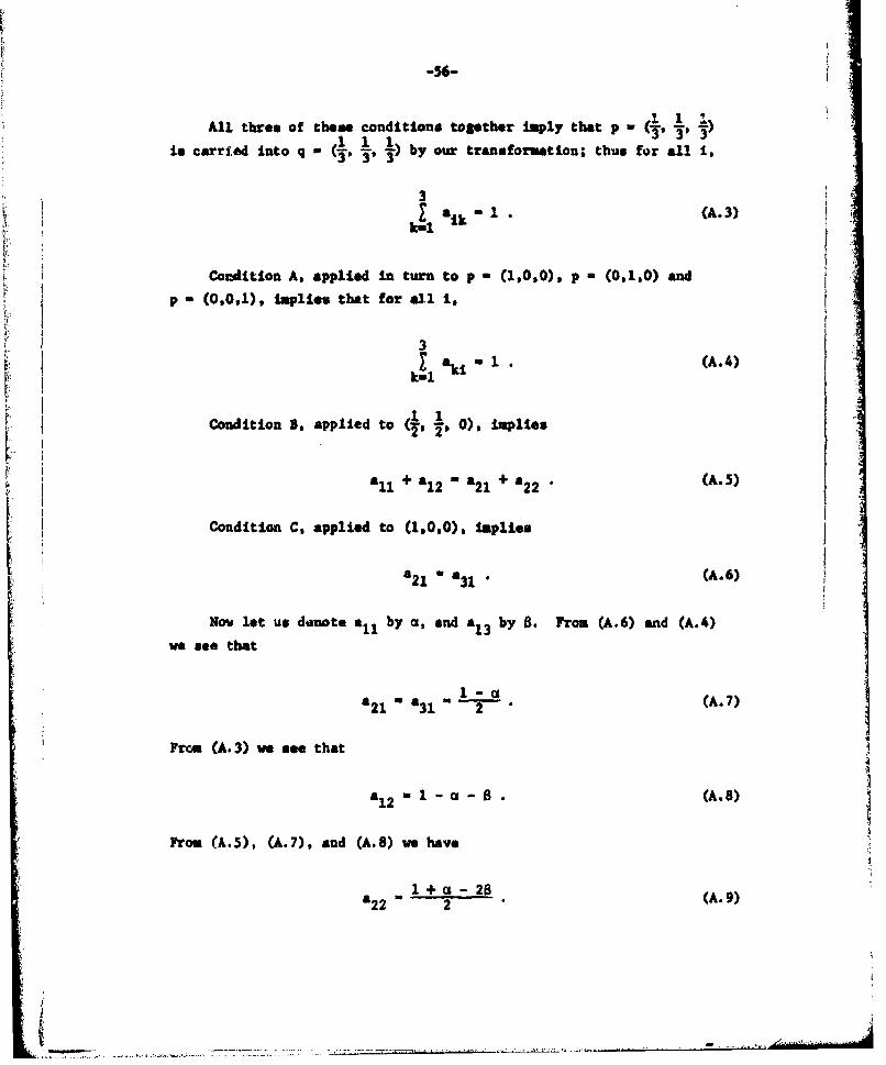
-56-

All three of these conditions together imply that p - (., 1 )

i. carried into q - (•. 1 , .) by our transformation; thus for all i,

3i•1 tk =1 .(A.3)

k-l

Condition A, applied in turn to p - (1,0,0), p - (0,1,0) and

p - (0,0,1), tmplies that for all t,

3a ki 1 (A.4)

Condition C, applied to (1,010), Implies

Condition C, applied to (1.0,0), Implies

a21 a 31 . (A.6)

Nov let us denote al1 by u, and £13 by 8. From (A.6) and (A.4)

ve see that

£21 " a3 1 -2 . (A.7)

Frcm (A.3) we see that

a12 -1-u-B. (A.8)

From (A.5), (A.7), and (A.8) we haveIV

I + 2 - (2 9)£22 2 "

Frou (A.8), (A.9), and (A.3) we derive

'23 (A.10)

Applying (A.4) now yields

+ a (A.)32 2 and 33 1 "20.

In mmaery, the application of normality and symmetry conditions

shows that system (A1) may be written

q, " axPl + (1 - a - 0) P2 + OP3

1•'-Pa + (l1 +- a- 2+2 * _2 PI 2 P2 + BP3 (A.12)

93 - - P " p -1+ 2 _.P2 + (1 - 2B)P 3

It is easy to see that these expressions are necessary and suf-ficient conditions for (A), (B), and (C) to hold.

The parameters a and B have an immediate interpretation, as follows.The requirement that p1 , P2 m P3 means that we are restricting ourattention to one-sixth of the "answer triangle" (the shaded area in theupper left-hand triangle of Fig. 24). The mapping (A.12) leaves thepoint (-1 ,) fixed, carries (1,0,0) into (a,0,0), and carries

of the shaded triangle, and by knowing what happens to them it is easy

to visualize what happens to all other points in the triangle. Figure24 includes three examples of what the mappings look like for dtfferentvalues of a and B.

2. NINI3IIZATION OF AThis section gives the formulas required to calculate values of

a and B that will minimize A, the quantity defined by (A.2). The der-ivation of these formulas is by taking the derivative of A with respect

i -58-

3 2 3 2

I I

2 3 2 2

Fig. 24- Effect of the linear transformation on the triangle p P>_ 2! P3for various values of a and 13

to a and B. We skip the intermediate steps In this routine calcula-

tion, and jump directly to our final formulas:

Ccoi CEO - Ca C•

'-o C0 -c C0 G

(A.13)

a Ca1. an - CI. Claamcoo C3 - COM Coo

The quantities appearing in these formulas are defined a& follows.

Let

"- P1 P 2 2 3 (A. 14)i ÷P -PI -a= a- L

l P 2 -,P 1 :4 P1 -

p3 2

The reader will note that

-J AA ai + A0 + C

I II I I A I

Nov we define

J-1 i-i s O J11 A4- A

n 3

Coa1-1 i i Ai

n n 3(A.16)

j1 I~ - - -

n n 3

0. ijJ-1 i-i I-i

-60-

Recall that I is the subscript of the probability ascribed to the

correct answer on the jth queation. Now the reader may be bothered

by the following question: suppose a respondent on the first questions

lists probabilities (0.4, 0.2, 0.4), and the third answer is lu fact

correct. We reorder the probabilities to get (0.4, 0.4, 0.2), but

what value do we take for I1? Should it be 1 or 2? It does not matter,

as far as calculating our coefficients a and B is concerned, for i

enters into the calculation only as a subscript for A's and B's; when

this ambiguity arises about whether i - 1 or I - 2, we have p1 - p2

and so A1! A2 and Bj Bj. Similarly, if there is ambiguity over

whetheri1 -2ori 1 3, we have A - Aand A B Because of the

symmetry built into Eq. (A.12), it also makes no difference which pos-

sible value of iJ we select (where ambiguity exists) in calculating

the total score awarded to the "transformed" estimates.

3. TRUNCATION AND NIMORALIZATION

The procedure above does not necessarily lead to a vector (qls

q2 ' q3 ) that is a proper probability vector. Although the q's will

sum to one, they will not necessarily fall between zero and one. We

truncate and renormalize in the obvious way:

(1, max (0, qj))q min =

Id

(A.17)3d " min (1, max (0, q J))

i-1

This truncation may seem rather arbitrary and ad hoc. Recall,

however, that it will take place only if the respondent underestimetes

his knowledge (and a and B do not fall between zero and one), a phenom-

enon that so far has occurred only rarely and with naive subjects.

Therefore, the use of a more sophisticated truncation and renormaliza-

tion routine hardly seems justified.

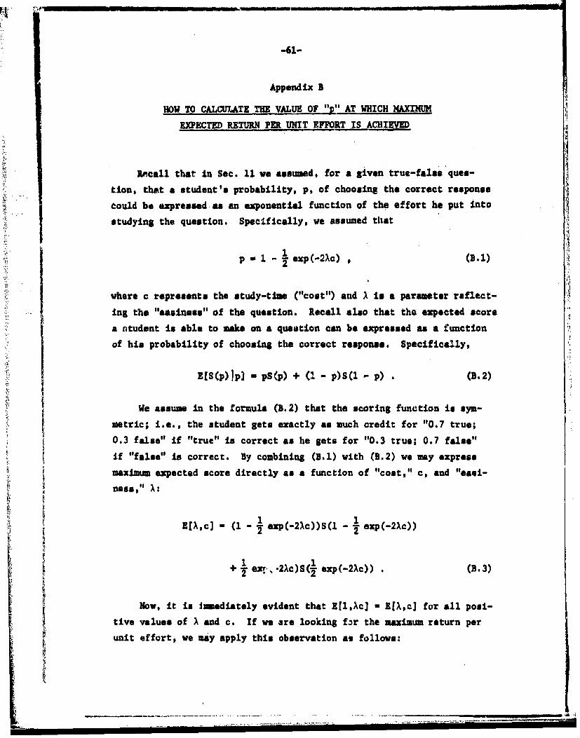
-61-

Appendix B

HOW TO CA1CULATE THE VALUE OF "v" AT WHICH MAXIMUM

EXPECTED RETURN PER UNIT EFFORTIS ACHIEVE

Recall that in Sec. 11 we assumed, for a given true-false ques-

tion, that a student's probability, p, of choosing the correct response

eould be expressed as an exponential function of the effort he put into

studying the question. Specifically, we assumed that

p- 1- exp(-2,c) , (3.1)

where c represents the study-time ("cost") and XL is a parameter reflect-

ing the "easiness" of the question. Recall also that the expected score

a ntudent is able to make on a question can be expressed as a function

of his probability of choosing the correct response. Specifically,

EL[SWp)jp -ps(p) + (1 -p)S(l p) . (B.2)

We assume in the formula (B.2) that the scoring function is sym-

metric; i.e., the student gets exactly as much credit for "0.7 true;

0.3 false" if "true" is correct as he gets for "0.3 true; 0.7 false"

if "false" is correct. By combining (1.1) with (B.2) we may express

maximum expected score directly as a function of "cost," c, and "ea'ui-

ness," A~:

E[A,cJ- (1 - exp(-2)Xc))S(l - .1 exp(-2Xc))1 2

+ ex.., -2Xc)S(t sxp(-2)c)) . (B-.3)

Now, it is Immediately evident that E[,Zlcj - E[X,c] for all posi-

tive values of A and c. If vs are looking far the maximum return per

unit effort, we may apply this observation as follows:

-62-

ma" c - XE~lc) - E max (B.4)Cao c cO , ckO cz c

In~~~~~~~~~~~~ othe wodi crprsnste)stta aiieIn other words, if cX represents the cost that maximizes-

then A~c -c 1 This is true, in an obvious sen,:.e, even if the c, areA

not unique. In our learning model, p depends on the product of X and

c. This is extremely convenient, for if we let pX - Xc,, we see that

P• pl. In other words, the maxim= return per uiit effort is achieved

on a given true-false question by studying that question until a given

probability of choosing the correct answer is achieved; and this

"ýmaatery level" (which we shall call p.) does not depend on the easi-

ness of the question, but only on the scoring function used. Thiscritical mastery level is thus a characteristic of the scoring func-

tion; presumably students will study harder when faced with a scoring

function with a high critical naatery level than they will when faced

with a scoring function having a low one.

If the scoring function is differentiable, elementary •1 ulus

may be used to calculate the value of p . One good way to do this isto use the chain rule, as follows:

!L(EIj( j ) 1P .1dE _1(B5

"dc"c c dp dc 2 (B.5)

log(2p)•-T~ple1: Lt 5p)1 log (2) "This is the loga~rithic scoring rule

normalized so that S(j) - 0 and S(l) - 1. Then

E p log(2p) + (1 - p) lop(2(1 -p)log 2

dr- 1°8(1 --' )d- log (B.6)dcp log 2

! - X exp(-2Xc) -2(l - p)Xdc"

-63-

Therefore,

c log(2) ' ) - c log 2(1 -p))

-p log(2p) + (1 - p log(2(1 - p)) • (3.7)

Since

c-,os2!. ] (B.8)2

we see that (B.7) may be expressed as

c log2 A( "" -l log(2(1 - p))(1 - p)

- p log2p - (1 - p) log(2(l - p)) . (B.9)EI

The aximum value of w- vil1 be achieved at the point where the

right-hand side of (B.9) iquals zero. Solving this transcendental

equation is very difficult by hand, but is easy (using the method of

false position or Newton's method) on any computer. The derivative

in (B.9) is zero at p-y; is positive for < p < 0.8910751 ... ; and

is negative for 0.8910751 ... < p. Thus the aximum expected score

per unit effort is achieved for p - 0.8910751 ....

Example 2: Let S(p) - 1 - 4(1 - p)2 This is the "quadratic scoring

system," or "Brier score," often used by meteorologists to evaluate

the quality of probabilistic weather predictions. In our case, weInormalize it so that e(-) - 0 and s(1) - 1. Then

E- (2p - 1)2

dEd- ap - 4 (B.10)

2(1 p)Xde

• • • . ...... ..... •...... .,.- ,.. -..-.....

-64-

So

c~. •c ) - c (8p - 4) 2 ( (1 p)X - (2p - 1)2dc a c

Using relation (3.8), we see that

C - •o1(2 - p) ( - p) (2p - (2p 1)

(B.12)

Simple calculation shows that the derivative in (B.12) is zero at

p - ; positive for < p < 0.857665933 ... ; and negative for p >

0.85766593 .... Thus the maximum expected score per unit effort against

the quadratic scoring system is achieved at p - 0.85766593 .... In

short, the quadratic scoring system is apparently slightly less effective

(theoretically) than the logarithmic scoring system in stimulating stu-

dents to work hard on individual questions.

Example 3: The techuiques of this appendix may also be applied to scor-

ing systems that are not admissible. For example, suppose a student is

approaching a true-false test that is to be marked and graded in the

traditional way (+1 for a right answer; -1 for a wrong one). Then If

a student has probability p e.f selecting the right answcr, his expected

score on the question will be p a (+1) + (1 - p) * (-1). We therefore

have

E -=2p- 1

dE2 (B.13)

AR 2(1 -p) A

Thus

2 d - c • 2 2 (1 - p))- (2p-l) . (1.14)

ac c

....--......... - . -~... ~ ', 9 '' ''

-65-

It follows that

2d a-Eý - -2(l p)log(2(l -p)) -(2p -1) (B.15)dc(

The derivative In (B.15) In negative for <' p < 1. It follows

that (_)is & maxium at p - .In other words, the uaxiinm returnper unit effort against a conventional true-false question Is achievedby putting forth an infiniteuimal amount of effort.

-66-

Appendix C

ALLWCATING STtUY EFFORT TO MAXIMZE PROFIT

In Appendix B we analyzed the problem of how much study would get

the muxiwm return per unit effort. Another approach to the question

of how students will be motivated to study is to suppose that study

effort and points pined on a test question can be measured In com-

mensurable terms. The student is then In the position of "purchasing"

expected score vith study effort. You night expect the student to

attempt to maxisize his "profit"; that is, to try to make the differ-

ence between the value of the score he expects to gain and the value

(to him) of the effort he expends in study. In short, he will try to

Maximize

B0A,c) - c . (C.1)

If the reward system is such that E is a differentiable function

of p, then this maximization problem may be solved by finding the point

at which the derivative is zero.

d ( c) dE d• 1 (C. 2)TC . - dp dc

We assume, as in Appendix B, that

1i

p =l- exp (-2),c) ((C.3)

dd-c- X exp(-2,c) - ,2(l - p)

Combining (C.2) with (C.3) we see that the derivative of profit

will be zero where

2dE" (C.4)2(l p) dp

I I II I I II I

-67-

Although we would ordinarily think of fixing A and then solving

for p (or what is the same thing, c), Expression (C.4) is such an easy

formula that the best way to derive numerical values seems to be to

regard p as a parameter and derive the maximum expected profit as a( + lo2M - 9). A. (p)

function of A by plotting the curve .E(p) + 21(p) '

Eample 1: Consider the logarithmic scoring system, S(p) log 2

Then we have

X(p) = 2(1 -p)[log(p/1 - p)j

; Z~~~(p) - - + p lon P + . (1 - 0 111o(l 9)( .5log 2

(1 - )log 2i(1 - p)(.c

+log 2

Carrying out these calculations yields the following values:

p lambda cost profit

0.99 7.542 0.25934 0.659860.98 4.453 0.36146 0.497100.97 3.323 0.42327 0.382330.96 2.726 0.46321 0.294490.95 2.354 0.48906 0.221540.94 2.099 0.50500 0.167560.93 1.914 0.51360 0.120480.92 1.774 0.51658 0.081240.91 1.664 0.51514 0.048390.90 1.577 0.51018 0.020820.89 1.507 0.50238 -0.002290.88 1.450 0.49226 -0.02163

Note that for p less than about 0.9 there is really no value of A

for which such a p is optimal, since it is better not to study at all

(and get zero profit) than to do any studying and get a negative profit.

Example 2: low let us turn to the quadratic scoring system, S(p)

1 -4 (p - 1)2.

, i -,

-68-

P 2(1 - p)[A( 2 p - 1)](C.6)

2R(p) - c (I -2p) + (1 - p) 4 (2p -)lo 2(1- p)

Carrying out these calculations leads to the following:

p lambda cost profit

0.99 12.755 0.15335 0.807050.98 6.510 0.24721 0.674390.97 4.433 0,31735 0.566250.96 3.397 0.37179 0.474610.95 2.778 0.41447 0.395530.94 2.367 0.44780 0.326600.93 2.076 0.47344 0.266160.92 1.860 0.49260 0.213000.91 1.694 0.50621 0.166190.90 1.563 0.51502 0.124980.89 1.457 0.51965 0.088750.88 1.371 0.52061 0.056990.87 1.299 0.51835 0.029250.86 1.240 0.51326 0.005140.85 1.190 0.50567 -0.01567

If X is less than about 1.2, It is better not to study at all, and

accept zero profit, for no finite amount of effort expended will lead

to a commensurate reward.

Example 3: As a final example, consider a normal true-false test.

This is not an admissible scoring system, but we can see that E(p) -

11

2p, 1 (p I). Thus

X(P) 4(1 -p)

(C.7)

1(p) - c - 2p - 1 + 2(1 - p)log 2(1 - p)

Computation yields the following:

-69-

p lambda cost profit

0. 95 5.000 0.23026 0.669740.90 2.500 0.32189 0.478110.85 1.667 0.36119 0.338810.80 1.250 0.36652 0.233480.75 1.000 0.34657 0.153430.70 0.833 0.30650 0.093500.65 0.714 0.24967 0.050330.60 0.625 0.17851 0.021490.55 0.556 0.09482 0.005180.50 0.500 0.0 0.0

If X c 0.5, then any positive amount of study is unremunerative.

i

..

i

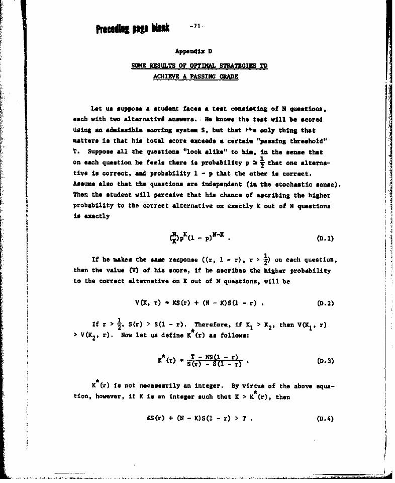
pM"Alg pgso u -71

Appendix D

SO" RESULTS O OPIRML STMATIHGIS TO

ACHIEVE A PASSING GRADE

Let us suppose & student faces a test consisting of N questions,

each with two alternativd answers.. He knows the test will be scored

asing an admissible scoring systm S, but that r'e only thing that

natters is that his total score exceeds a certaiu "passing threshold"

T. Suppose all the questions "look alike" to him, in the sense that

on each question he feels there is probability p ' k that one alterna-

tive is correct, and probability 1 - p that the other is correct.

Assume also that the questions are independent (in the stochastic sense).Then the student will perceive that his chance of ascribing the higher

probability to the correct alternative on exactly K out of N questions

is exactly

(XNK(1 . p)N- . (D.1)

m If he wakes the same response ((r, 1 - r), r > 1) on each question,then the value (V) of his score, if he ascribes the higher probability

to the correct alternative on K out of N questions, will be

V(K, r) - KS(r) + (N - K)S(l - r) . (D.2)

If r > ½, S(r) > S(1 - r). Therefore, if K1 > K2, then V(Kl, r)

> V(K2 , r). Now let us define K (r) as follows:

K*(r) (D.3)

K (r) is not necessarily an integer. By virtue of the above equa-

tion, however, if K is an integer such that K > KX(r), then

KS(r) + (N - K)S(l - r) > T (D.4)

J...i'-~~ii.i~t~.j4~2f ~ , ___

-72

Therefore, the student will maximize his probability of "passing the

test" (i.e., getting a score greater than T) if he selects that r which

minimizes K (r). I assert that the optimum value of r (which we shall

call r*) is that r which satisfies the equation,

r SOr+(I-r)S(l-r (D.5)

By substituting (D.5) in (D.3) we see that

- r r (D. 6)N

Now consider some r r*, r > We will show that K*(r) > K*(r*),

thus proving that r is an optimal response. By definition of what an

admissible scoring system is, we know that

Kr K *r K (r*NL S (*)+ 1 SU r) N S(r)

(D. 7)

+ (1 K-r ~ r)

From this, and (D.3), we deduce

K (r)S(r) + (N - K*(r))S(l - r) - T > K*(r*)S(r)

(D.8)

+ (N - *(r*))s(l - r)

Thus

K (r)[S(r) -S(U- ) K*(r)[S(r) -S(l- r)]

K (r) - K*(r*). (D.9)

The fact that the solution to (D.5) is an optimal response in this

setting is a striking illustration of the fact that nonlinear utility

for score may destroy the admissible property of a scoring system, for

!,A

-73

Eq. (D.5) does not depend upon the student's subjective probability p

at all!

It is interesting to note, by the way, that the optimal total test

strategy may not involve making the same response on all questions, evenwhen the student's subjective probabilities on all questions are the

smne. For example, if T - S(l) and he is completely uninformed (p -on all questions, then he viii secure a 50 percent chance of passing

by making a (1,0) response on one question and a ( -5 1) response on allthe rest. This is manifestly a better chance than he can secure by any

strategy that calls for the same (r, 1 - r) response on every question.

!I

.. .. . .~ . 0, , . , 0 , , " ... . . . . . . . . .. .. i -. . .

MWlp In -77-

1. Brown, T. A., and H. Shuford, Jr., Quantifving• o L rtainty Intoj ~NwwrcaZ ProbabiZities for. the Reporti~ng of InteZligenoe, The

Rand Corporation, R-1185-ARPA, 1973.

2. Grayson, C., Decisions Under Thwertintzj: Droiltin Decisions byjOiZ and Gas Opera.tor, Harvard Business School, Division of Ra-search, Boston, hss.., 1950.

3. Savage, L. J., "Elicitstion of Personal Probabilities and Expecta-tions," JournaZ of the American StatisticaZ Association, Vol. 66,1971, pp. 783-801.

4. Sibley, V. L., A Pm'totijpe Computer PFog2'a for' Interactive Computer'-Ad4inisatred Ad#niaibZe ProbabiZity Measurwaent, The Rand Corpora-tion, R-1258-ARPA, 1973.

55. Shannou, C. I., and V. Weaver, The MathenaticaZ Yheo•y of Cwnmi-cation, University of Illinois Press, Urbana, Ill., 1949.

6. Shuford, H., Jr., A. Albert, and H. E. .Massengill, "AdmissibleProbability measuuremnt Procedures," Payaohometrika, Vol. 31,1966, pp. 125-145.

7. Brown, T. A., .Frobabilistic Po2'eoaets and Reproducing Sorinng Sys-ten#, The Rand Corporation, RJ4-6299-ARPA, June 1970.

,I

•1 I I I I U u n g ,