Disparity statistics in natural scenesDepartment of Electrical and Computer Engineering,The University of Texas at Austin, Austin, TX, USAYang Liu

Department of Electrical and Computer Engineering,The University of Texas at Austin, Austin, TX, USAAlan C. Bovik

Department of Psychology,The University of Texas at Austin, Austin, TX, USALawrence K. Cormack

Binocular disparity is the input to stereopsis, which is a very strong depth cue in humans. However, the distribution ofbinocular disparities in natural environments has not been quantitatively measured. In this study, we converted distancesfrom accurate range maps of forest scenes and indoor scenes into the disparities that an observer would encounter, givenan eye model and fixation distances (which we measured for the forest environment, and simulated for the indoorenvironment). We found that the distributions of natural disparities in these two kinds of scenes are centered at zero, havehigh peaks, and span about 5 deg, which closely matches the macaque MT cells’ disparity tuning range. These ranges arefully within the operational range of human stereopsis determined psychophysically. Suprathreshold disparities (910 arcsec)are common rather than exceptional. There is a prevailing notion that stereopsis only operates within a few meters, but ourfinding suggests that we should rethink the role of stereopsis at far viewing distances because of the abundance ofsuprathreshold disparities.

Keywords: stereopsis, binocular disparity, stereoacuity, stereo upper limit, Panum’s fusion area

Citation: Liu, Y., Bovik, A. C., & Cormack, L. K. (2008). Disparity statistics in natural scenes. Journal of Vision, 8(11):19, 1–14,http://journalofvision.org/8/11/19/, doi:10.1167/8.11.19.

Introduction

Stereopsis is the ability to see depth using retinaldisparities, which are the differences in relative imageposition of scene points on the two retinae. It is widelythought (Palmer, 1999) that stereopsis does not operatebeyond a few meters because the retinal disparityproduced by a given depth interval decreases dramaticallywith distance. Further, binocular disparity is a relative cueand must be scaled by absolute distance information. Themost obvious sources of this information, convergenceand accommodation, cease to be effective beyond a fewmeters, so it is not surprising that stereopsis is assumed tobehave similarly. Nobody, however, has measured thedisparities actually occurring outdoors and examined theirrelationship to the visual system. It is easy to show thatsuprathreshold disparities can indeed occur at far viewingdistances (e.g., von Helmholtz, 1962; Tyler, 1991), but ifthey are abundant or even in the majority rather than beinga curious exception, then we should perhaps rethink therole of stereopsis in both ordinary vision and in primateevolution.To determine disparities in the natural world, we must

have two pieces of information: the real distance fromeach direction where the incoming light strikes the retinaand the point of binocular fixation. For the former, laser

range scanning technology suits this task well. Severalresearchers collected range maps in the real world(Huang, Lee, & Mumford, 2000; Potetz & Lee, 2003;Yang & Purves, 2003a). Yang and Purves (2003b) placedtheir laser scanner at a height of 1.65 m, which is a typicaleye height of a male adult. We computed disparitydistributions in natural scenes using available range mapsfrom Yang and Purves (2003b) and distributions ofbinocular fixation points that we either measured empiricallyor simulated. In this paper, we concentrated our analysis onthe horizontal plane at eye height because the vast majorityof our observers’ fixations were near this plane.

Range map data

We formatted the range data into a right hand worldcoordinate system with metric unit, where the x axis goesfrom left to right, the y axis goes from down to up, and thez axis points toward the viewer. In each range map, theorigin of the coordinate system is the location of the laserscanner.To calculate exact disparities, we must first have an

optical model of the human eye. We approximated thehuman eye as a perfect sphere with its center at its nodalpoint (Le Grand, 1980). With an interpupillary distance of

Journal of Vision (2008) 8(11):19, 1–14 http://journalofvision.org/8/11/19/ 1

doi: 10 .1167 /8 .11 .19 Received July 17, 2007; published August 29, 2008 ISSN 1534-7362 * ARVO

0.065 m, we assume that the nodal points of the twoidentical eye balls are located at (j0.0325, 0, 0) and(0.0325, 0, 0), and the observer is looking at the negativedirection of the z axis.Instead of computing the 3D projection on the retinal

sphere, we only consider the projection in a particular 2Dsituation, which is the horizontal great circle of the retinalsphere. All the scene points on the XZ plane are projectedon the horizontal great circle with different horizontaldisparities but zero vertical disparities. A scene point’shorizontal disparity can be accurately calculated when weknow the coordinates of the current fixation and its ownposition.Figure 1 is a top view of the XZ plane when the two

eyes are fixating on a point F (xf, yf, zf). We define thefixation distance to be the distance between the fixationpoint F and Oc, which is also the midpoint between thetwo eyes. To simplify the computation, we assume the twoeyes have a midsagittal fixation, which means xf = 0 andyf = 0. By doing so, we can use the fixation distance zf torepresent a fixation. The disparity of point P can bespecified by:

d ¼ "rj"l ¼ !j8 ð1Þ

where

! ¼ 2 atanðj0:0325=zf Þ; ð2Þ

8 ¼ atanjxpj0:0325

zp

� �jatan

jxp þ 0:0325

zp

� �: ð3Þ

Each range map is a geometrical description of theworld by a laser scanner centered at Oc. If we think of thelaser scanner as the cyclopean eye, then its retina is hit bylaser beams at all directions with the same angularsampling step size. Of course, this geometrical descriptionof the world may not be the same when the laser scanneris located at the left eye’s position Ol, or the right eye’sposition Or. But since the interpupillary distance is muchsmaller than the distances in the range maps, it isreasonable to assume that the range maps are valid fortwo eyes at Ol and Or.From Equation 1 we can see that the disparity is de-

cided by zf, xp, yp, and zp. The range map gives xp, yp,and zp. We must decide the position of the fixation pointF(0, 0, zf) beforehand to calculate the disparity. In orderto simulate the human fixation in the forest scenes, weconducted the following experiment to collect humanfixation distances in an environment similar to the one inwhich the range data were collected.

Empirical fixation distancedistribution

Three observers, one female and two male, with normalor corrected to normal vision, were asked to walk in awooded park near the campus of the University of Texasat Austin. (Pilot observations showed that some peoplelook at the ground a great deal of the time. Our threeobservers did not. Obviously, the effects of the groundplan are very interesting and relevant to stereopsis andbinocular vision, but in this paper we wanted to concen-trate on disparities at large viewing distances along thehorizontal meridian.)Two experimenters followed the observer. The first

experimenter, who did not look at the observer whilewalking, timed random intervals between 2 and30 seconds. At the end of each random interval, “time”was called and the observer reported the current locus offixation (The observers found it to be easy after a fewtrials). The line-of-sight distance to the indicated regionwas then measured using a laser rangefinder fordistances larger than 15 meters. A measuring wheelwas used for distances smaller than 15 meters. Wecollected 100 fixation distances for each observer for a

Figure 1. The geometry of binocular disparity computation. Whenthe observer is fixating at point F, the vergence angle is !. Anotherpoint P has two projections on two retinae. The angle between theleft visual axis FOl and the left projection line POl is "l, and theangle between the right visual axis FOr and the right projectionline POr is "r. We define the binocular disparity to be d = "r j "l.Theoretically, if the point P is inside the ideal horopter defined bythe current fixation F, the disparity of P is negative (crossed).Otherwise it is positive (uncrossed). When P is exactly located onthe horopter, its two projections are on the corresponding retinalpoints, which yield 0 disparity.

Journal of Vision (2008) 8(11):19, 1–14 Liu, Bovik, & Cormack 2

total of 300 binocular fixation samples. We selected 255out of the 300 fixation distances by omitting all distancessmaller than 2 m, which served to eliminate the rareoccasions when the observers were looking at the groundat their feet. We denote the 255 fixation distances as d1,d2, I d255. These fixation distances range from 2.7 m to123.8 m.Figure 2 shows the distribution of fixation distances we

obtained (top right), along with the distribution ofdistances present in the range data (top left). Bothdistributions are roughly log-normal, which can be seen

as a linear relationship when the quantiles of the log of thedata are plotted against equal quantiles from the standardnormal distribution (middle). Similarly, when the quan-tiles of the range data are plotted against equal quantilesof the fixation data, the trend is roughly linear indicatingthat the two distributions are very similar in shape. Thisindicates that, effectively, observers are selecting fixationdistances in accord with their prevalence in the environ-ment. If this is true, then such an observer could be easilymodeled for the purposes of computing disparity distribu-tions, a point to which we will return below.

Figure 2. The human fixation distance (A) are roughly log normal distributed and matched well with the scene distances (B) at eye level.See text for details. The insets in the upper row show the scene distances converted to angular units that, for some readers, may facilitatecomparisons with the subsequent figures.

Journal of Vision (2008) 8(11):19, 1–14 Liu, Bovik, & Cormack 3

The computation of naturalbinocular disparity

Previous studies show humans generally fixate onrelevant objects during daily visual tasks, such as makinga sandwich (Hayhoe, Shrivastava, Mruczek, & Pelz, 2003)and making tea (Land, Mennie, & Rusted, 1999).Similarly, our observers always reported fixating on aspecific object, generally on or near the horizontal plane.We used the following method to combine our humanfixation distances with the range maps.For each fixation distance di, we went through the

23 forest range maps to find a matched distance d onthe horizontal plane, with a criterion of the error (di j d) /di G 5%. This matching process gave us (hopefully) a goodintuitive association between the range maps and ourfixation data, the idea being “Given that observers generallyfixate on objects, and given that this observer was fixating ata distance d, where could he or she have been plausiblylooking in the range data?” After we found the matched

distance d, we placed a virtual observer with the midpointbetween two eyes located at the origin Oc and directlyfacing the direction of the matched distance d.Figure 3 shows this process schematically for fixations

1, 2, and 255. The top row shows each fixation along withthe 631 scene points within a horizontal 90-deg anglecentered on fixation (the horizontal resolution of the rangemaps is about 0.143 deg). The next row shows thedisparities computed for each of these points, and thethird row shows the histograms of these disparities foreach fixation point (column). Finally, the data werecombined across fixations to yield the overall disparitydistribution shown at the bottom.This distribution of disparities is shown in greater detail

in Figure 4A. This plot represents our best estimate of thedistribution of angular disparities available to an observerlooking straight ahead in a natural outdoor woodedenvironment. The peak is very near zero, but the span isover 4.5 deg. The maximum of disparity is 1.24 deg,which corresponds to the nearest fixation at about 2.66 mand a farthest scene point at about 160 m; the minimum isj3.30 deg, which corresponds to the farthest fixation at

Figure 3. This flowchart shows the process of disparity computation. We find a scene distance matching every human fixation distanceand chose its T45-deg neighborhood to compute disparities. Each 90-deg neighborhood contributes 631 disparities to the overallhistogram. The total histogram contains 255 � 631 = 160905 disparities.

Journal of Vision (2008) 8(11):19, 1–14 Liu, Bovik, & Cormack 4

about 124 m and a nearest scene point at about 1.2 m. Themean is roughly zero deg (4.07 arcmin), and the standarddeviation is about 0.37 deg (22.2 arcmin). The kurtosis is5.57, which is much larger than that of the Gaussian(kurtosis = 0), indicating that there are too manydisparities near zero to be consistent with a Gaussiandisparity distribution. Indeed, it is apparent that theGaussian red curve is not a satisfactory fit by eye. Wealso fitted the Laplace distribution, whose probabilitydensity function is f(xª2, b) = exp (jªx j 2ª/b)/2b, tothe disparity data using the MLE (maximum likelihoodestimation) method. The fit is clearly better. Moreover, aplot of log-density vs. disparity is shown in Figure 4B, andthe roughly linear flanks are consistent with the Laplacedistribution (though the kurtosis Laplace distribution is 3,which is still substantially lower than our obtained valueof close to 6). Crucially, however, 98% of the distributioncomprises disparity values greater than T10 arcsec (a largebut not unreasonable stereothreshold).As mentioned above, the distributions of environmental

distance and fixation distance are strikingly similar, whichis what would be obtained if, for our purposes, observerswere selecting a random visual direction, and fixating thenearest object along that direction (in other words, this isthe simplest behavior that would lead to a match betweenthe range and fixation distributions shown in Figure 2). Totest this, we recomputed the distribution of disparitiesfrom the range maps using a simulated observer instead ofour empirical distribution of fixation distances. Thissimulated observer first selected a random (uniform)azimuth for head orientation over T120 deg (i.e., halfthe 330-deg field of view of the rangefinder minus theT45-deg field over which we compute disparities) and thenselected the coordinate corresponding to the nearest objectin that direction (i.e., the range returned by the rangefinderin that direction) as the fixation point. We did this a totalof 255 times (selecting a random range map each time) toyield the same number of disparity estimates as above(255 � 631). The resulting disparity distribution is shown

in Figure 5 and is qualitatively very similar to that inFigure 4. The dark blue line in Figure 5 shows the bestfitting Laplace distribution for these disparities, while thedashed blue line shows the best fitting Laplace for thedisparities estimated using the human fixation data (i.e.,re-plotted from Figure 4A). The inset shows the quantile–quantile (Q–Q) plot of the two estimated disparitydistributions. The striking agreement (the linearity of theQ–Q plot) indicates that, for the present purposes at least,we can use a model that selects the nearest point along arandom visual direction as a fixation point to generate areasonable approximation of human fixation distances.Obviously, this is not what human observers do, but itproduces the same distribution of fixation distances overthe long run.A main point of this study is that the distribution of

disparities in large-scale (outdoor) environments is largelysuprathreshold, and therefore a potential stimulus to

Figure 4. (A) The distribution of binocular disparity derived from 23 forest range maps. The red curve is the best fitting Gaussian on thedata. It is visually apparent that the distribution is non-Gaussian because of the higher peak and heavier tails. (B) The distribution betweenT1 deg shows a good linearity using semi-log plot.

Figure 5. The disparity distribution from nearest fixations withuniformly distributed orientations, the solid blue line shows thebest fitting Laplace, and the dashed blue line is the re-plot of thebest fitting Laplace of the disparity distribution from human fixationdistances. The inset shows the quantile–quantile plot of the twodistributions. The good linearity is prominent.

Journal of Vision (2008) 8(11):19, 1–14 Liu, Bovik, & Cormack 5

stereopsis. It might be argued that the suprathresholddisparities arise largely from very distant objects whenfixation is very near, or from very near objects whenfixation is at infinity. In Figure 6, we separate thehistogram into two sub-histograms, which correspond to

fixation distances larger than the median fixation distanceof 15 m (red) and those smaller than 15 m (blue). For farfixations, there is a very high peak of near zero disparitiescorresponding to continuous local far neighborhoodaround the fixations and also a considerably long tail ofcrossed disparities from nearer scene points. For nearerfixations, the peak around zero is much lower. This isbecause the relative disparity between two points of samedistance interval is larger when the absolute distances ofthe two points are closer to an observer. Because of thepiecewise continuous structure of natural scenes, a pointin the 90-deg scene matched with a nearer fixationdistance is more likely to reside in a nearer localneighborhood containing the fixation point, and vice versawith farther fixation distances. After these scene distanceshave been converted to disparities, the disparities in thenearer scenes differ from those in the farther scenessignificantly as Figure 6 shows. But we should stress thatthe difference between the red and blue plots in Figure 6 isultimately caused by different fixation distances. It is theupper (915 m) and lower (G15 m) fixation distances thatpartition the matched scenes into two different groups andyield the different disparity distributions in Figure 6.

Figure 6. The shape of disparity distribution changes with fixationdistance.

Figure 7. (A) The mean of disparity distributions at different eccentricities from forest scenes (circles) and indoor scenes (squares).(B) The standard deviations of two disparity distributions at different eccentricity. (C) The 95% ranges of two disparity distributionsat different eccentricities.

Journal of Vision (2008) 8(11):19, 1–14 Liu, Bovik, & Cormack 6

We also examined the relationship between sampleddisparities and horizontal eccentricity. Figures 7A and 7Bshow the mean (circles and red line) and standarddeviation (circles and red line) of the disparity distributionas a function of horizontal eccentricities (using 5-degeccentricity bins). Figure 7C (circles and red line) showsthe 95% range of the distribution (disparities between the97.5% percentile and 2.5% percentile) against eccentric-ities. The monotonic increase of the mean and standarddeviation is prominent. Figure 8A shows the pdfs of thedisparities at T13, T9, T5, and T1 deg. It is obvious to seethe distributions are all unimodal, roughly peaked nearzero, and become broader as the eccentricity increases.The increase of standard deviation and span of the

disparity distribution is easy to understand since the worldis piecewise continuous. With eccentricity growing,peripheral scene points are less likely to be located onthe same object or surface as the fixation point, whichresults a larger range of disparity values. Anotherinteresting observation is that the mean disparity alsoseems to increase with eccentricity, which indicates thatthe peripheral points tend to have positive (far) disparities.Does this also indicate that peripheral locations aregenerally farther away than straight-ahead fixations interms of absolute distance?1 It is unclear how this couldbe the case in the current study given that, even if therewere some systematic orientation bias in the originalrange data, it is difficult to imagine how this couldpropagate to the disparity data given the randomnessinherent in our simulations. Nevertheless, we verified thestationarity of the range data (as a whole) with respect toorientation by computing the range distributions (and themeans and standard deviations) at many orientations in theoriginal data and, indeed, the mean range, the standarddeviation, and (as far as we could tell) the shape ofthe range distribution were independent of orientation.The only thing remaining that could have produced theorientation dependence was the nature of the disparitycalculation, specifically, the VM circle. Referring toFigure 1, assume that the fixation F is such that the meandisparity along OcF is zero. Given the independence ofthe range data, this condition will hold (at least approx-

imately) for any other fixation point on the iso-distancecircle. Thus, if fixation were to remain at F, then the meandisparity at any eccentricity will be shifted by thedisparity between the VM circle and the iso-distancecircle at that eccentricity. This disparity shift is plotted asthe red dashed line in Figure 7A. The agreement is goodgiven the standard deviations associated with the data, andthe remaining discrepancy is probably due to the partic-ular sample of ranges we acquired. Note also that thesubjective horopter measured by psychophysical methodsis a little different from the VM circle (Howard &Rogers, 1995) and is generally between the VM circle andthe frontal parallel plane located at the fixation point.Thus, the effective dependence of mean disparity oneccentricity should be less in practice than estimated here.

Discussion

Relationship between different environmentsand natural disparity distribution

While environments such as room and car interiorsprobably had a minimal impact on primate evolution, theyundoubtedly provide a large amount of input to both themature and developing human binocular system. Fortu-nately, Yang and Purves (2003b) also collected range datafrom 27 indoor scenes at Duke University. The scannersetting was the same as in the scanning of the forestscenes. These indoor range maps represent descriptions ofthe distances of a 330 � 80 field of view from theperspective of a person with an eye-height of 1.65 m intypical indoor scenes like classrooms, halls, corridors, etc.In order to get a rough approximation of the disparity

distribution of indoor scenes, we took advantage of theobservation (above) that a simple algorithm that selectsthe nearest point along a random direction as the fixationpoint produces a very human-like distribution of fixationdistances. Again, we are certainly not claiming that this iswhat people actually do; we only note that, over many

Figure 8. Disparity distributions at different eccentricities in (A) forest scenes and (B) indoor scenes.

Journal of Vision (2008) 8(11):19, 1–14 Liu, Bovik, & Cormack 7

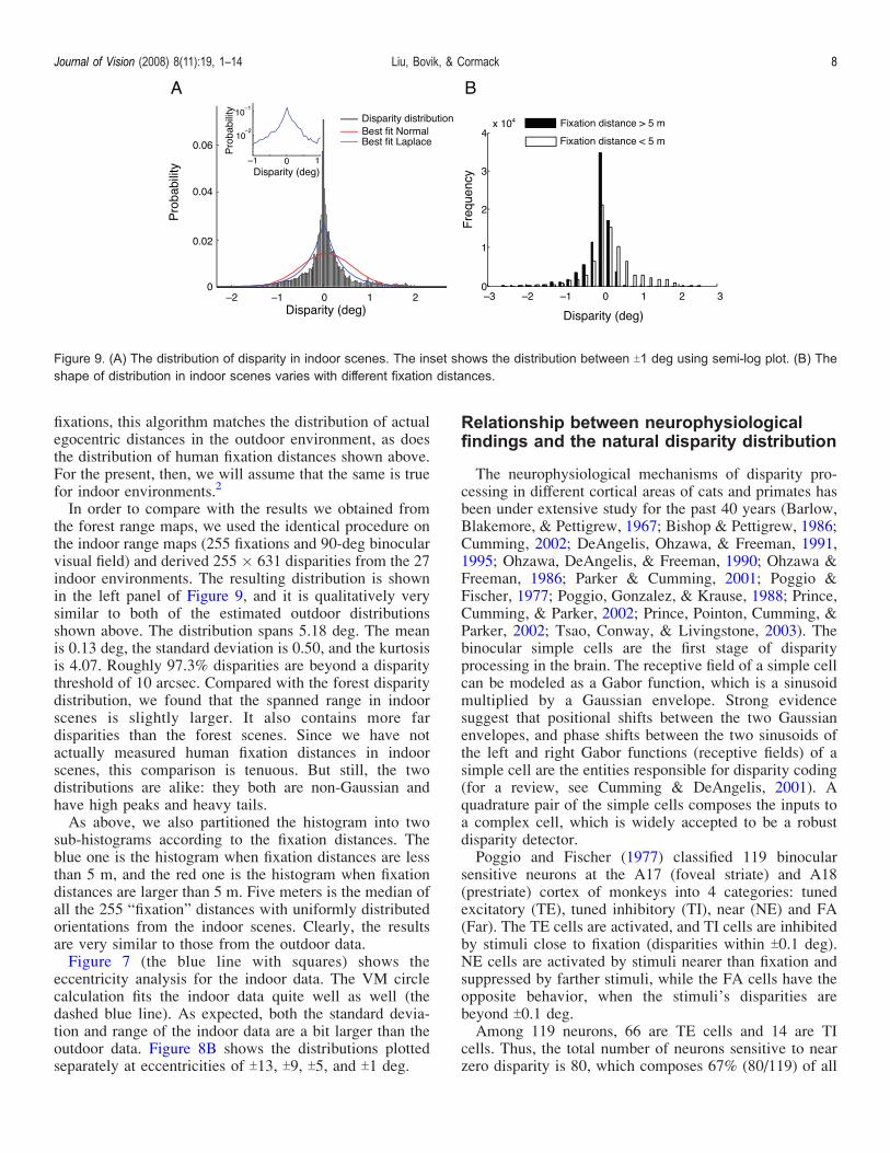
fixations, this algorithm matches the distribution of actualegocentric distances in the outdoor environment, as doesthe distribution of human fixation distances shown above.For the present, then, we will assume that the same is truefor indoor environments.2

In order to compare with the results we obtained fromthe forest range maps, we used the identical procedure onthe indoor range maps (255 fixations and 90-deg binocularvisual field) and derived 255 � 631 disparities from the 27indoor environments. The resulting distribution is shownin the left panel of Figure 9, and it is qualitatively verysimilar to both of the estimated outdoor distributionsshown above. The distribution spans 5.18 deg. The meanis 0.13 deg, the standard deviation is 0.50, and the kurtosisis 4.07. Roughly 97.3% disparities are beyond a disparitythreshold of 10 arcsec. Compared with the forest disparitydistribution, we found that the spanned range in indoorscenes is slightly larger. It also contains more fardisparities than the forest scenes. Since we have notactually measured human fixation distances in indoorscenes, this comparison is tenuous. But still, the twodistributions are alike: they both are non-Gaussian andhave high peaks and heavy tails.As above, we also partitioned the histogram into two

sub-histograms according to the fixation distances. Theblue one is the histogram when fixation distances are lessthan 5 m, and the red one is the histogram when fixationdistances are larger than 5 m. Five meters is the median ofall the 255 “fixation” distances with uniformly distributedorientations from the indoor scenes. Clearly, the resultsare very similar to those from the outdoor data.Figure 7 (the blue line with squares) shows the

eccentricity analysis for the indoor data. The VM circlecalculation fits the indoor data quite well as well (thedashed blue line). As expected, both the standard devia-tion and range of the indoor data are a bit larger than theoutdoor data. Figure 8B shows the distributions plottedseparately at eccentricities of T13, T9, T5, and T1 deg.

Relationship between neurophysiologicalfindings and the natural disparity distribution

The neurophysiological mechanisms of disparity pro-cessing in different cortical areas of cats and primates hasbeen under extensive study for the past 40 years (Barlow,Blakemore, & Pettigrew, 1967; Bishop & Pettigrew, 1986;Cumming, 2002; DeAngelis, Ohzawa, & Freeman, 1991,1995; Ohzawa, DeAngelis, & Freeman, 1990; Ohzawa &Freeman, 1986; Parker & Cumming, 2001; Poggio &Fischer, 1977; Poggio, Gonzalez, & Krause, 1988; Prince,Cumming, & Parker, 2002; Prince, Pointon, Cumming, &Parker, 2002; Tsao, Conway, & Livingstone, 2003). Thebinocular simple cells are the first stage of disparityprocessing in the brain. The receptive field of a simple cellcan be modeled as a Gabor function, which is a sinusoidmultiplied by a Gaussian envelope. Strong evidencesuggest that positional shifts between the two Gaussianenvelopes, and phase shifts between the two sinusoids ofthe left and right Gabor functions (receptive fields) of asimple cell are the entities responsible for disparity coding(for a review, see Cumming & DeAngelis, 2001). Aquadrature pair of the simple cells composes the inputs toa complex cell, which is widely accepted to be a robustdisparity detector.Poggio and Fischer (1977) classified 119 binocular

sensitive neurons at the A17 (foveal striate) and A18(prestriate) cortex of monkeys into 4 categories: tunedexcitatory (TE), tuned inhibitory (TI), near (NE) and FA(Far). The TE cells are activated, and TI cells are inhibitedby stimuli close to fixation (disparities within T0.1 deg).NE cells are activated by stimuli nearer than fixation andsuppressed by farther stimuli, while the FA cells have theopposite behavior, when the stimuli’s disparities arebeyond T0.1 deg.Among 119 neurons, 66 are TE cells and 14 are TI

cells. Thus, the total number of neurons sensitive to nearzero disparity is 80, which composes 67% (80/119) of all

Figure 9. (A) The distribution of disparity in indoor scenes. The inset shows the distribution between T1 deg using semi-log plot. (B) Theshape of distribution in indoor scenes varies with different fixation distances.

Journal of Vision (2008) 8(11):19, 1–14 Liu, Bovik, & Cormack 8

cells. There are 22 (19%) FA cells and 11 (9%) NE cells.They also found that all neurons’ preferred disparities arelimited within T1 deg. Although the 4 category classi-fication of neurons is rather rough and has been challengedby newer findings in psychophysics and physiology(Cormack, Stevenson, & Schor, 1993; Stevenson, Cormack,Schor, & Tyler, 1992), it still yields a quantitativemeasurement of the proportions of disparity tuning in V1.Prince, Cumming, et al. (2002) studied 180 neurons in

V1 of macaque monkeys with strong binocular disparityselectivity. Their data support a continuum of disparitytuning instead of 4 discrete categories. However, they stillapplied the same simple criterion by Poggio and Fischer(1977) to the 180 neurons. Their results were in goodagreement with Poggio and Fisher: 69 (38%) are TEneurons, 29 (16%) are TI neurons, 38 (21%) are NEneurons and 44 (25%) are FA neurons.Now consider the disparity distribution in the 23 forest

range maps (Figure 4). Using the 0.1-deg criterion andonly considering the disparities within the T5 degeccentricity limit found in both results (Poggio & Fischer,1977; Prince, Cumming, et al., 2002), 17% of the naturaldisparities are larger than 0.1 deg (FA), 22% are smallerthanj0.1 deg (NE), and 61% are within T0.1 deg (TE/TI).In the 27 indoor range maps, 12% of the disparities arelarger than 0.1 deg, 11% are smaller than j0.1 deg, and77% are within T0.1 deg.The general agreement between the natural disparity

distribution and the physiological data of V1 are veryinteresting. As Figures 4 and 9 show, 97.5% of thedisparities in forest scenes and 93% of the disparities in

indoor scenes are within T1 deg. This means that most ofthe natural disparities are within the encoding range of theV1 cells. Figure 10 shows that more than half of naturaldisparities within T5 deg eccentricity are betweenT0.1 deg, which is consistent with the V1 cells. The forestscenes contain a slightly greater number of near disparitiesthan far disparities. However, the indoor scenes containalmost same number of far disparities and near disparities.Of course, as our previous results show, the distribution ofdisparities has a dependency on fixation distances. Nearfixation distances produces more far (uncrossed, positive)disparities, and far fixation distances produces more near(crossed, negative) disparities. It seems that the disparitiesin the forest and indoor scenes are roughly symmetric, notthe same as V1, which has more far tuned neurons thannear tuned neurons. However, it is debatable to concludethat more V1 neurons are tuned to far than to near givenonly two studies (Poggio & Fisher, 1977; Prince,Cumming, et al., 2002), and it is also debatable that the23 forest scenes and 27 indoor scenes are the most relevantenvironments in V1 evolution. Perhaps those elements ofthe environment that are within reach of the primate armcontribute more to the development of V1 tuning, but wedo not know what the disparity distribution in smalldistances looks like without available range maps.It is known that the size of receptive fields increases

with retinal eccentricity, and the spatial frequency ofreceptive fields decreases with retinal eccentricity (Wilson& Sherman, 1976). In the well-accepted binocular energymodel proposed by Ohzawa and Freeman (1986), acomplex cell receives inputs from a quadrature pair ofsimple cells. The complex cell’s disparity tuning curve isdecided by the size and spatial frequency of the simplecells (Ohzawa & Freeman, 1986; Qian & Zhu, 1997; Zhu& Qian, 1996). Peripheral neurons with larger receptivefields and lower spatial frequencies can encode disparitiesat a wider range, but with coarser resolution. As is shownby a recent report on V1 (see Figure 11 in Prince,Cumming, et al., 2002), the disparity tuning curves dobecome continuously coarser and wider as the eccentricitygrows.Another study on binocular receptive fields and eccen-

tricity (Joshua & Bishop, 1970) on anesthetized catsshowed that the standard deviation of receptive fielddisparity, which is a term similar to the preferred disparityof the neuron, also increases with eccentricity. Table 1lists the standard deviation of the receptive field disparityfrom Joshua and Bishop (1970), and the standard devia-tion of the natural disparity distribution in the forestscenes and the indoor scenes in different eccentricitygroups. The qualitative agreement among the two columnsis obvious. Again, this clearly shows that the property ofdisparity sensitivity in V1 may match the distribution ofnatural disparities.Recent physiological findings suggest that V1 is not

directly responsible for high level depth perception(Cumming & Parker, 2000). DeAngelis and Uka (2003)

Figure 10. The percentage of binocularly tuned V1 Neurons fromPoggio and Fisher (1977), Prince, Cumming, et al. (2002), thepercentage of natural disparities within T5-deg eccentricity fromthe forest scenes and from the indoor scenes. NE represents theneurons tuned to near disparities smaller than j0.1 deg. TE andTI represent neurons tuned to disparities within T0.1 deg. FArepresent far disparities larger than 0.1 deg. The yellow bars andred bars show the proportions of the disparities in our disparitydistributions that can excite the NE, TE and TI, and FA cells,respectively.

Journal of Vision (2008) 8(11):19, 1–14 Liu, Bovik, & Cormack 9

studied the MT (V5) area of awake macaque monkeys.They found that MT neurons are more significantly tunedto horizontal disparities than V1 cells and have a broaderrange of disparity tuning. Unlike the T1 deg limit of theV1 cells reported by Poggio and Fischer (1977) andPrince, Cumming, et al. (2002), the range of MT’sdisparity tuning covers about 6 deg centered at 0. Thedisparity tuning range of MT, shown in Figure 11A, ismore closely matched with natural disparity distributions,which also spans 4–5 deg, although it would appearthat MT oversamples large disparities relative to theirprevalence in our distributions. This is also shown by the

Q–Q plots in Figures 11C and 11D; there is excellentagreement over a roughly 2-deg central range, but the MTdata show heavier tails. An interesting property of the MTdisparity tuning is the preference of negative (near)disparities. Although the majority of the MT cells arestill tuned to smaller disparities near zero, there arenoticeably more (61%) neurons tuned to negative (near)disparities than positive (far) disparities, which is just thereverse of the V1 cells, and is also different from theroughly symmetric natural disparity distribution. Figure 11Bshows the proportions the disparities in the forest scenesand indoor scenes respectively, compared with the MT

Figure 11. (A) The distribution of the preferred disparities of 471 MT neurons. (B) The disparity percentage of the MT neurons, the forestscenes, and the indoor scenes. We used the same T0.1-deg criterion here as in Figure 10. You may notice that the shape of naturaldisparity bar plot is different from that of Figure 10. It is because that we chose the disparities within a 30-deg eccentricity to match the MTneurons’ eccentricity range instead of the 5-deg eccentricity range of V1. (C) The Q–Q plot of the disparity distribution in the 23 forestrange maps against the preferred disparities of 471 MT neurons. (D) The Q–Q plot of the disparity distribution in the 27 indoor range mapsagainst the preferred disparities of 471 MT neurons.

EccentricityStandard deviation of spread of

receptive field disparitiesStandard deviation of the natural binocular

disparities in the 23 forest scenesStandard deviation of the natural binocular

disparities in the 27 indoor scenes

0–4 deg 0.50 deg (90 cells) 0.23 deg 0.29 deg4–8 deg 0.76 deg (74 cells) 0.26 deg 0.32 deg8–12 deg 0.79 deg (39 cells) 0.35 deg 0.40 deg12–16 deg 0.90 deg (10 cells) 0.41 deg 0.46 deg

Table 1. Changes in horizontal receptive field disparities with horizontal retinal eccentricities, adapted from Joshua and Bishop (1970).

Journal of Vision (2008) 8(11):19, 1–14 Liu, Bovik, & Cormack 10

neurons, based on the same T0.1-deg criteria but within a30-deg eccentricity to match the MT neurons’ eccentricityrange. The MT’s deviation from the natural disparitydistribution and the V1 neurons is obvious.What causes the deviation of MT’s disparity tuning

from V1’s? We assume that V1 is specialized for disparityencoding instead of depth perception. If V1 is simply anencoder, then its job should be loyally conveying thedisparity information to higher cortical areas for furtherdisparity processing. Thus, the disparity tuning of V1 cellsshould exactly reflect the disparity distribution in thenatural environment, nothing more, nothing less. How-ever, not every disparity is equally important to the well-being of the creature. From an ecological and evolutionalpoint of view, a nearer object is more important to thecreature, since it means either a reachable fruit or anapproaching danger. It is imaginable that higher corticalareas such as MT weight the input from V1 differentlyaccording to their importance.

Relationship between psychophysicalfindings and the natural disparity distribution

The operational range of stereopsis is determined bytwo limits:

1. depth discrimination threshold (stereoacuity) and2. upper disparity limit. Various methods have been

used to measure the two limits.

The obtained results are different, given different experimentdesigns. But it is commonly believed that the depthdiscrimination is the best at the foveal center and with zerodisparity and decreases with growing eccentricity andpedestal disparity. The upper disparity limit increases witheccentricity and stimulus size.Ogle (1952) studied the limit of stereopsis by moving

one rod in depth away from the fixation. There are threestereo perception levels:

1. strong depth perception in the Panum’s fusionalarea (T5 arcmin at the fovea), where objects arefused,

2. strong depth perception with diplopia, and3. vague depth perception with diplopia.

He called the first two patent stereopsis, and the thirdqualitative stereopsis.Ogle found the range of patent stereopsis extends to

about T10 arcmin at the fovea. There is a clear disparity–depth relationship in this area, which makes fine depthjudgment possible. Beyond the T10 arcmin limit, theperformance of judging the stimulus to be nearer orfurther than the fixation is still above chance, but the finedisparity–depth relationship is lost. The range of qual-

itative stereopsis at fovea is about T15 arcmin. There is noreliable depth perception beyond the qualitative stereopsisrange. At the periphery, the range of reliable depthperception is much larger. For example, patent stereopsisextends to about 70 arcmin and qualitative stereopsisabout 2 deg at a 6-deg eccentricity.Westheimer and Tanzman (1956) found that the limit of

convergent (uncrossed) disparity is about 6 deg anddivergent (uncrossed) disparity about 10 deg. Blakemore(1970) studied the range of stereopsis using a small fixationpoint and briefly exposed, vertical slit-shaped targets atdifferent eccentricities and pedestal disparities. He foundthat the upper limit for reliable qualitative localization of aslit as nearer or further than the fixation is 4–7 deg ofabsolute disparity in a convergent direction and 9–12 deg ina divergent direction near the fovea. Even larger absolutedisparities can be recognized as the eccentricity of the slitsincreases. Landers and Cormack (1997) also found thatreliable disparity discrimination is well beyond 1 deg.The width of the disparity distribution in the 23 forest

scenes is about 4.5 deg, which is covered by the rangefound by Blakemore (1970). Apparently, the distributionof disparities depends on the distance distributions in theenvironments. Blakemore’s experiments had a viewdistance of only 43.7 cm, which is significantly smallerthan the distances in a forest. This could be one reasonthat the disparity limit he measured is larger than therange of the disparity distribution.Blakemore (1970) studied the disparity discrimination

thresholds at different eccentricities and different pedestaldisparities. He found that the best stereoacuity is achievedat the zero eccentricity and at the fixation. There is a lossof stereoacuity as the eccentricity grows, where thedisparities are more likely to be large. Our findings showthat binocular disparities in the natural world have a largerstandard deviation as the eccentricity grows.Tyler (1973) measured the sensitivity function for the

disparity modulation and found that the stereoacuitypeaked at a disparity modulation frequency about 1 cpd.For lower disparity modulation frequency, both the lowerand higher disparity limits were elevated. Prince andRogers (1998) measured the sensitivity function fordisparity modulation at different eccentricities. Theyfound that the sensitivity decreased with eccentricity, butinterestingly, the peak sensitivity to disparity modulationalways happened at the same frequency at all eccentric-ities, with cortical magnification factor taken into account.In a very recent study, Hibbard (2007) also modeled the

statistics of disparity in a similar way as we did, but he useda collage sphere model (spheres randomly distributed atdifferent spatial locations) instead of actual range data tocalculate the disparity distribution. He also found thedisparity-eccentricity dependency and the Laplace-likeshape of the disparity distribution, which are very similarto our results. Our results thus indicate that Hibbard’s modelproduces an accurate statistical description of disparityinformation for at least two common environments.

Journal of Vision (2008) 8(11):19, 1–14 Liu, Bovik, & Cormack 11

Conclusion

By computing disparities from actual range data, wefound that the distribution of binocular disparities in forestscenes and indoor scenes from Yang and Purves’s (2003b)range map database is highly peaked at 0 deg and spansseveral degrees. The range of the disparity distribution isfully covered by the range of macaque MT cells’ (DeAngelis& Uka, 2003) disparity tuning. The proportion of thedistribution is qualitatively consistent with the proportionof the disparity tuned V1 neurons (Figure 10). We arefully aware that our distribution is not the canonicalmeasurement of the disparities across all tasks andenvironments. But it does seem to be a robust estimateof the disparities that an observer is likely to encounter inboth large scale (outdoor) and small scale (indoor)environments when gaze is roughly horizontal.Simoncelli and Olshausen (2001) pointed out that the

evolution and development of a biological visual system isdriven by three fundamental factors: (1) the tasks that thevisual system must perform, (2) the computationalcapabilities and limitations of the neurons, and (3) theliving environment of the organism. In this paper, we triedto correlate the disparity distribution in the naturalenvironments with other research areas in stereopsis inan attempt to integrate these points. Examples of thisintegrated perspective are biologically compatible stereo-psis models (Read, Parker, & Cumming, 2002; Tsai &Victor, 2003). These models tried to solve depth percep-tion with current computational models (DeAngelis et al.,1991; Ohzawa et al., 1990; Qian & Zhu, 1997) ofbinocular neurons. Read et al. (2002) assumed a non-Gaussian, zero-favoring distribution of the disparity as aBayesian prior. Our disparity distribution supports herassumption quite well and can also serve as a moreaccurate priori probability in a Bayesian framework ofstereo correspondence.Finally, we point out that the most up-to-date laser

scanning technology offers co-registered distance andluminance maps (Potetz & Lee, 2003). It is even moreinteresting to look at the joint distribution of luminancefeatures and disparity features in the natural world if thistechnology is combined with a fixation selection scheme,which will greatly enhance our understanding of the stereocorrespondence and disparity processing.

Acknowledgments

This research was supported by NSF Grant ITR-0427372. We thank Zhiyong Yang and Dale Purves forsharing their range maps. We also thank KalpanaSeshadrinathan for her useful comments and proofreading.

Commercial relationships: none.Corresponding author: Yang Liu.Email: young76@mail.utexas.edu.Address: Department of Electrical and Computer Engi-neering, The University of Texas at Austin, TX 78712.

Footnotes

1If anything, the opposite is probably true when

navigating, considering the nature of paths, roads, andhallways.

2Of course people deploy their fixations differently

(in some sense) for different tasks in different environ-ments, and this may influence the shape of the distributionof fixation distances relative to the distribution of environ-mental distances, but until we can simultaneously measureranges and fixations in the same environment and co-register the data, we will proceed under the aboveassumption.

References

Barlow, H. B., Blakemore, C., & Pettigrew, J. D. (1967).The neural mechanism of binocular depth discrim-ination. The Journal of Physiology, 193, 327–342.[PubMed] [Article]

Bishop, P. O., & Pettigrew, J. D. (1986). Neuralmechanisms of binocular vision. Vision Research,26, 1587–1600. [PubMed]

Blakemore, C. (1970). The range and scope of binoculardepth discrimination in man. The Journal of Physiol-ogy, 211, 599–622. [PubMed] [Article]

Cormack, L. K., Stevenson, S. B., & Schor, C. M. (1993).Disparity-tuned channels of the human visual system.Visual Neuroscience, 10, 585–596. [PubMed]

Cumming, B. G. (2002). An unexpected specialization forhorizontal disparity in primate primary visual cortex.Nature, 418, 633–636. [PubMed]

Cumming, B. G., & DeAngelis, G. C. (2001). Thephysiology of stereopsis. Annual Review of Neuro-science, 24, 203–238. [PubMed]

Cumming, B. G., & Parker, A. J. (2000). Local disparitynot perceived depth is signaled by binocular neuronsin cortical area V1 of the Macaque. Journal ofNeuroscience, 20, 4758–4767. [PubMed] [Article]

DeAngelis, G. C., Ohzawa, I., & Freeman, R. D. (1991). Depthis encoded in the visual cortex by a specialized receptivefield structure. Nature, 352, 156–159. [PubMed]

DeAngelis, G. C., Ohzawa, I., & Freeman, R. D. (1995).Neuronal mechanisms underlying stereopsis: How do

Journal of Vision (2008) 8(11):19, 1–14 Liu, Bovik, & Cormack 12

simple cells in the visual cortex encode binoculardisparity? Perception, 24, 3–31. [PubMed]

DeAngelis, G. C., & Uka, T. (2003). Coding of horizontaldisparity and velocity by MT neurons in the alertmacaque. Journal of Neurophysiology, 89, 1094–1111.[PubMed] [Article]

Hayhoe, M. M., Shrivastava, A., Mruczek, R., & Pelz, J. B.(2003). Visual memory and motor planning in anatural task. Journal of Vision, 3(1):6, 49–63, http://journalofvision.org/3/1/6/, doi:10.1167/3.1.6. [PubMed][Article]

Hibbard, P. B. (2007). A statistical model of binoculardisparity. Visual Cognition, 15, 149–165.

Howard, I. P., & Rogers, B. J. (1995). Binocular visionand stereopsis. New York: Oxford University Press.

Huang, J., Lee, A. B., & Mumford, D. (2000). Statistics ofrange images. Paper presented at CVPR, 2000.

Joshua, D. E., & Bishop, P. O. (1970). Binocular singlevision and depth discrimination. Receptive field dis-parities for central and peripheral vision and binoc-ular interaction on peripheral single units in cat striatecortex. Experimental Brain Research, 10, 389–416.[PubMed]

Land, M., Mennie, N., & Rusted, J. (1999). The roles ofvision and eye movements in the control of activitiesof daily living. Perception, 28, 1311–1328. [PubMed]

Landers, D. D., & Cormack, L. K. (1997). Asymmetriesand errors in perception of depth from disparitysuggest a multicomponent model of disparity pro-cessing. Perception & Psychophysics, 59, 219–231.[PubMed]

Le Grand, Y. (1980). Physiological optics. New York:Springer-Verlag.

Ogle, K. N. (1952). On the limits of stereoscopic vision.Journal of Experimental Psychology, 44, 253–259.[PubMed]

Ohzawa, I., DeAngelis, G. C., & Freeman, R. D. (1990).Stereoscopic depth discrimination in the visualcortex: Neurons ideally suited as disparity detectors.Science, 249, 1037–1041. [PubMed]

Ohzawa, I., & Freeman, R. D. (1986). The binocularorganization of complex cells in the cat’s visual cortex.Journal of Neurophysiology, 56, 243–259. [PubMed]

Palmer, S. E. (1999). Vision scienceVphotons to phenom-enology. Cambridge, MA: MIT Press.

Parker, A. J., & Cumming, B. G. (2001). Corticalmechanisms of binocular stereoscopic vision. Pro-gress in Brain Research, 134, 205–216. [PubMed]

Poggio, G. F., & Fischer, B. (1977). Binocular interactionand depth sensitivity in striate and prestriate cortex of

behaving rhesus monkey. Journal of Neurophysiol-ogy, 40, 1392–1405. [PubMed]

Poggio, G. F., Gonzalez, F., & Krause, F. (1988). Stereo-scopic mechanisms in monkey visual cortex: Binocularcorrelation and disparity selectivity. Journal of Neuro-science, 8, 4531–4550. [PubMed] [Article]

Potetz, B., & Lee, T. S. (2003). Statistical correlationsbetween two-dimensional images and three-dimensionalstructures in natural scenes. Journal of the OpticalSociety of America A, Optics, Image Science, andVision, 20, 1292–1303. [PubMed]

Prince, S. J., Cumming, B. G., & Parker, A. J. (2002).Range and mechanism of encoding of horizontaldisparity in macaque V1. Journal of Neurophysiol-ogy, 87, 209–221. [PubMed] [Article]

Prince, S. J., Pointon, A. D., Cumming, B. G., & Parker,A. J. (2002). Quantitative analysis of the responses ofV1 neurons to horizontal disparity in dynamicrandom-dot stereograms. Journal of Neurophysiology,87, 191–208. [PubMed] [Article]

Prince, S. J., & Rogers, B. J. (1998). Sensitivity todisparity corrugations in peripheral vision. VisionResearch, 38, 2533–2537. [PubMed]

Qian, N., & Zhu, Y. (1997). Physiological computation ofbinocular disparity. Vision Research, 37, 1811–1827.[PubMed]

Read, J. C., Parker, A. J., & Cumming, B. G. (2002). Asimple model accounts for the response of disparity-tuned V1 neurons to anticorrelated images. VisualNeuroscience, 19, 735–753. [PubMed]

Simoncelli, E. P., & Olshausen, B. A. (2001). Naturalimage statistics and neural representation. AnnualReview of Neuroscience, 24, 1193–1216. [PubMed]

Stevenson, S. B., Cormack, L. K., Schor, C. M., & Tyler,C.W. (1992). Disparity tuning in mechanisms of humanstereopsis. Vision Research, 32, 1685–1694. [PubMed]

Tsai, J. J., & Victor, J. D. (2003). Reading a population code:A multi-scale neural model for representing binoculardisparity. Vision Research, 43, 445–466. [PubMed]

Tsao, D. Y., Conway, B. R., & Livingstone, M. S. (2003).Receptive fields of disparity-tuned simple cells inmacaqueV1.Neuron, 38, 103–114. [PubMed] [Article]

Tyler, C. W. (1973). Stereoscopic vision: Cortical limi-tations and a disparity scaling effect. Science, 181,276–278. [PubMed]

Tyler, C. W. (1991). Cyclopean vision. In D. Regan (Ed.),Vision and visual dysfunction. Binocular vision(vol. 9, pp. 38–74). London: Macmillan.

von Helmholtz, H. (1962). Treatise on physiologicaloptics (vol. III). New York: Dover.

Journal of Vision (2008) 8(11):19, 1–14 Liu, Bovik, & Cormack 13

Westheimer, G., & Tanzman, I. J. (1956). Qualitativedepth localization with diplopic images. Journal ofthe Optical Society of America, 46, 116–117.[PubMed]

Wilson, J. R., & Sherman, S. M. (1976). Receptive-fieldcharacteristics of neurons in cat striate cortex:Changes with visual field eccentricity. Journal ofNeurophysiology, 39, 512–533. [PubMed]

Yang, Z., & Purves, D. (2003a). A statistical explanationof visual space. Nature Neuroscience, 6, 632–640.[PubMed]

Yang, Z., & Purves, D. (2003b). Image/source statistics ofsurfaces in natural scenes. Network, 14, 371–390.[PubMed]

Zhu, Y. D., & Qian, N. (1996). Binocular receptive fieldmodels, disparity tuning, and characteristic disparity.Neural Computation, 8, 1611–1641. [PubMed]

Journal of Vision (2008) 8(11):19, 1–14 Liu, Bovik, & Cormack 14