discrete sampling and integration for the ai practitionermeel/slides/cmv-aaai17.pdf• naive...
TRANSCRIPT

DiscreteSamplingandIntegrationfortheAIPractitioner
Supratik Chakraborty,IITBombayKuldeepS.Meel,RiceUniversityMosheY.Vardi,RiceUniversity

Agenda
Part1:BooleanSatisfiability Solving(Vardi)
Part2(a):Applications(Chakraborty)
CoffeeBreak
Part2(b):PriorWork(Chakraborty)
Part3:Hashing-basedApproach(Meel)

Discrete Sampling and Integration for the AIPractitioner
Part I: Boolean Satisfiability Solving
Supratik Chakraborty, IIT BombayKuldeep S. Meel, Rice University
Moshe Y. Vardi, Rice University
Boolean Satisfiability
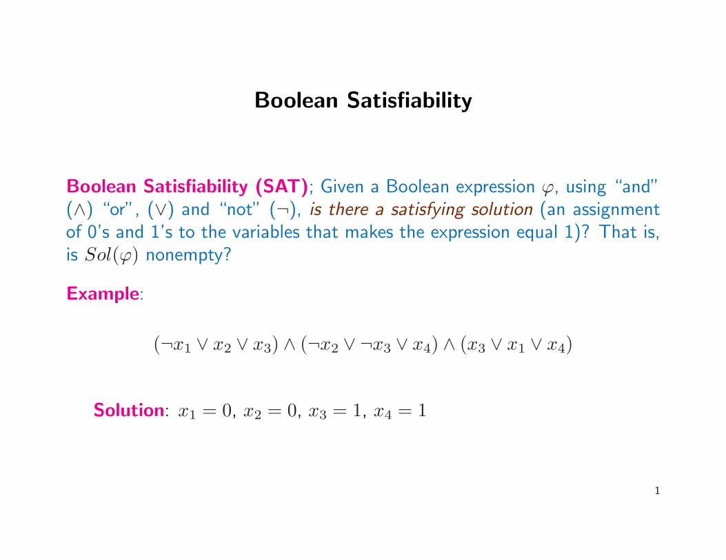
Boolean Satisfiability (SAT); Given a Boolean expression ϕ, using “and”(∧) “or”, (∨) and “not” (¬), is there a satisfying solution (an assignmentof 0’s and 1’s to the variables that makes the expression equal 1)? That is,is Sol(ϕ) nonempty?
Example:
(¬x1 ∨ x2 ∨ x3) ∧ (¬x2 ∨ ¬x3 ∨ x4) ∧ (x3 ∨ x1 ∨ x4)
Solution: x1 = 0, x2 = 0, x3 = 1, x4 = 1
1
Discrete Sampling and Integration
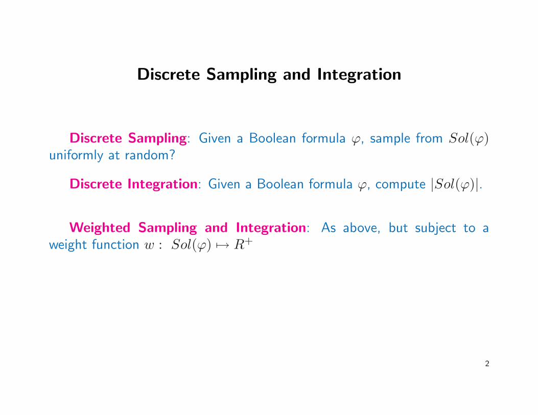
Discrete Sampling: Given a Boolean formula ϕ, sample from Sol(ϕ)uniformly at random?
Discrete Integration: Given a Boolean formula ϕ, compute |Sol(ϕ)|.
Weighted Sampling and Integration: As above, but subject to aweight function w : Sol(ϕ) 7→ R+
2

Basic Theoretical Background
Discrete Integration: #SAT
Known:
1. #SAT is #P-complete.
2. In practice, #SAT is quite harder than SAT.
3. If you can solve #SAT, then you can sample uniformly using self-reducibility.
Desideratum: Solve discrete sampling and integration using a SAT solver.
3

Is This Time Different? The Opportunities andChallenges of Artificial Intelligence
Jason Furman, Chair, Council of Economic Advisers, July 2016:
“Even though we have not made as much progress recently on otherareas of AI, such as logical reasoning, the advancements in deeplearning techniques may ultimately act as at least a partial substitutefor these other areas.”
4

P vs. NP : An Outstanding Open Problem
Does P = NP?
• The major open problem in theoretical computer science
• A major open problem in mathematics
– A Clay Institute Millennium Problem– Million dollar prize!
What is this about? It is about computational complexity – how hard it isto solve computational problems.
5

Rally To Restore Sanity, Washington, DC, October 2010
6

Computational Problems
Example: Graph – G = (V,E)
• V – set of nodes• E – set of edges
Two notions:
• Hamiltonian Cycle: a cycle that visits every node exactly once.• Eulerian Cycle: a cycle that visits every edge exactly once.
Question: How hard it is to find a Hamiltonian cycle? Eulerian cycle?
7

Figure 1: The Bridges of Konigsburg
8

Figure 2: The Graph of The Bridges of Konigsburg
9

Figure 3: Hamiltonian Cycle
10

Computational Complexity
Measuring complexity: How many (Turing machine) operations does ittake to solve a problem of size n?
• Size of (V,E): number of nodes plus number of edges.
Complexity Class P : problems that can be solved in polynomial time – nc
for a fixed c
Examples:
• Is a number even?• Is a number square?• Does a graph have an Eulerian cycle?
What about the Hamiltonian Cycle Problem?
11

Hamiltonian Cycle
• Naive Algorithm: Exhaustive search – run time is n! operations
• “Smart” Algorithm: Dynamic programming – run time is 2n operations
Note: The universe is much younger than 2200 Planck time units!
Fundamental Question: Can we do better?
• Is HamiltonianCycle in P?
12

Checking Is Easy!
Observation: Checking if a given cycle is a Hamiltonian cycle of agraph G = (V,E) is easy!
Complexity Class NP : problems where solutions can be checked inpolynomial time.
Examples:
• HamiltonianCycle• Factoring numbers
Significance: Tens of thousands of optimization problems are in NP!!!
• CAD, flight scheduling, chip layout, protein folding, . . .
13

P vs. NP
• P : efficient discovery of solutions• NP : efficient checking of solutions
The Big Question: Is P = NP or P 6= NP?
• Is checking really easier than discovering?
Intuitive Answer: Of course, checking is easier than discovering, soP 6= NP !!!
• Metaphor: finding a needle in a haystack• Metaphor: Sudoku• Metaphor: mathematical proofs
Alas: We do not know how to prove that P 6= NP .
14

P 6= NP
Consequences:
• Cannot solve efficiently numerous important problems• RSA encryption may be safe.
Question: Why is it so important to prove P 6= NP , if that is what iscommonly believed?
Answer:
• If we cannot prove it, we do not really understand it.• May be P = NP and the “enemy” proved it and broke RSA!
15
P = NP
S. Aaronson, MIT: “If P = NP , then the world would be a profoundlydifferent place than we usually assume it to be. There would be no specialvalue in ‘creative leaps,’ no fundamental gap between solving a problem andrecognizing the solution once it’s found. Everyone who could appreciatea symphony would be Mozart; everyone who could follow a step-by-stepargument would be Gauss.”
Consequences:
• Can solve efficiently numerous important problems.• RSA encryption is not safe.
Question: Is it really possible that P = NP?
Answer: Yes! It’d require discovering a very clever algorithm, but ittook 40 years to prove that LinearProgramming is in P .
16
Sharpening The Problem
NP -Complete Problems: hardest problems is NP
• HamilatonianCycle is NP -complete! [Karp, 1972]
Corollary: P = NP if and only if HamiltonianCycle is in P
There are thousands of NP -complete problems. To resolve the P = NPquestion, it’d suffice to prove that one of them is or is not in P .
17

History
• 1950-60s: Perebor Project – Futile effort to show hardness of searchproblems.
• Stephen Cook, 1971: Boolean Satisfiability is NP-complete.• Richard Karp, 1972: 20 additional NP-complete problems– 0-1 Integer
Programming, Clique, Set Packing, Vertex Cover, Set Covering,Hamiltonian Cycle, Graph Coloring, Exact Cover, Hitting Set, SteinerTree, Knapsack, Job Scheduling, ...– All NP-complete problems are polynomially equivalent!
• Leonid Levin, 1973 (independently): Six NP-complete problems• M. Garey and D. Johnson, 1979: “Computers and Intractability: A Guide
to NP-Completeness” - hundreds of NP-complete problems!• Clay Institute, 2000: $1M Award!
18

Boole’s Symbolic Logic
Boole’s insight: Aristotle’s syllogisms are about classes of objects, whichcan be treated algebraically.
“If an adjective, as ‘good’, is employed as a term of description, let usrepresent by a letter, as y, all things to which the description ‘good’is applicable, i.e., ‘all good things’, or the class of ‘good things’. Letit further be agreed that by the combination xy shall be representedthat class of things to which the name or description represented byx and y are simultaneously applicable. Thus, if x alone stands for‘white’ things and y for ‘sheep’, let xy stand for ‘white sheep’.
19

Boolean Satisfiability
Boolean Satisfiability (SAT); Given a Boolean expression, using “and”(∧) “or”, (∨) and “not” (¬), is there a satisfying solution (an assignmentof 0’s and 1’s to the variables that makes the expression equal 1)?
Example:
(¬x1 ∨ x2 ∨ x3) ∧ (¬x2 ∨ ¬x3 ∨ x4) ∧ (x3 ∨ x1 ∨ x4)
Solution: x1 = 0, x2 = 0, x3 = 1, x4 = 1
20

Complexity of Boolean Reasoning
History:
• William Stanley Jevons, 1835-1882: “I have given much attention,therefore, to lessening both the manual and mental labour of the process,and I shall describe several devices which may be adopted for saving troubleand risk of mistake.”
• Ernst Schroder, 1841-1902: “Getting a handle on the consequencesof any premises, or at least the fastest method for obtaining theseconsequences, seems to me to be one of the noblest, if not the ultimategoal of mathematics and logic.”
• Cook, 1971, Levin, 1973: Boolean Satisfiability is NP-complete.
21
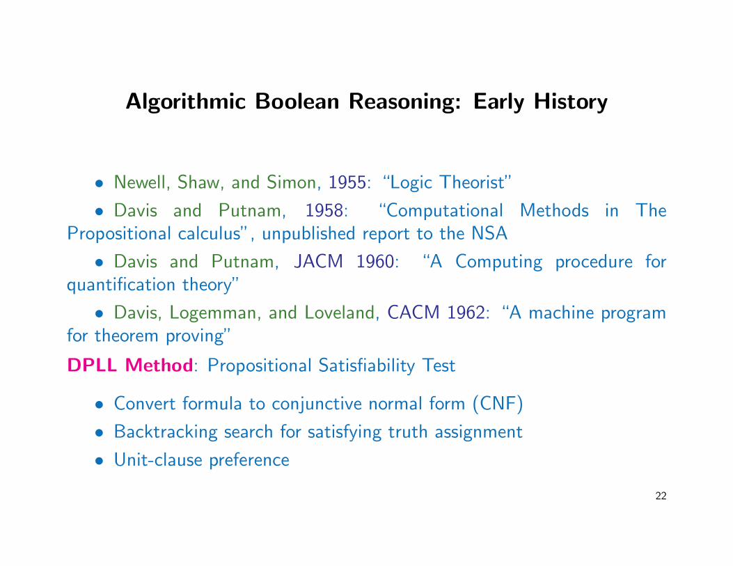
Algorithmic Boolean Reasoning: Early History
• Newell, Shaw, and Simon, 1955: “Logic Theorist”
• Davis and Putnam, 1958: “Computational Methods in ThePropositional calculus”, unpublished report to the NSA
• Davis and Putnam, JACM 1960: “A Computing procedure forquantification theory”
• Davis, Logemman, and Loveland, CACM 1962: “A machine programfor theorem proving”
DPLL Method: Propositional Satisfiability Test
• Convert formula to conjunctive normal form (CNF)
• Backtracking search for satisfying truth assignment
• Unit-clause preference
22

Modern SAT Solving
CDCL = conflict-driven clause learning
• Backjumping
• Smart unit-clause preference
• Conflict-driven clause learning
• Smart choice heuristic (brainiac vs speed demon)
• Restarts
Key Tools: GRASP, 1996; Chaff, 2001
Current capacity: millions of variables
23
S. A. Seshia 1
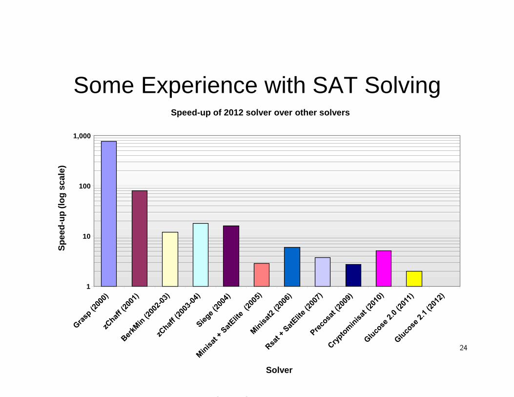
Some Experience with SAT Solving Sanjit A. Seshia
Speed-up of 2012 solver over other solvers
1
10
100
1,000
Solver
Sp
ee
d-u
p (
log
sc
ale
)
Figure 4: SAT Solvers Performance%labelfigure
24

Knuth Gets His Satisfaction
SIAM News, July 26, 2016: “Knuth Gives Satisfaction in SIAM vonNeumann Lecture”
Donald Knuth gave the 2016 John von Neumann lecture at the SIAMAnnual Meeting. The von Neumann lecture is SIAM’s most prestigiousprize.
Knuth based the lecture, titled ”Satisfiability and Combinatorics”, onthe latest part (Volume 4, Fascicle 6) of his The Art of ComputerProgramming book series. He showed us the first page of the fascicle,aptly illustrated with the quote ”I can’t get no satisfaction,” from theRolling Stones. In the preface of the fascicle Knuth says ”The story ofsatisfiability is the tale of a triumph of software engineering, blendedwith rich doses of beautiful mathematics”.
25

SAT Heuristic – Backjumping
Backtracking: go up one level in the search tree when both Booleanvalues for a variable have been tested.
Backjumping [Stallman-Sussman, 1977]: jump back in the search tree,if jump is safe – use highest node to jump to.
Key: Distinguish between
• Decision variable: Variable is that chosen and then assigned first c andthen 1− c.
• Implication variable: Assignment to variable is forced by a unit clause.
Implication Graph: directed acyclic graph describing the relationshipsbetween decision variables and implication variables.
26

Smart Unit-Clause Preference
Boolean Constraint Propagation (BCP): propagating values forced byunit clauses.
• Empirical Observation: BCP can consume up to 80% of SAT solvingtime!
Requirement: identifying unit clauses
• Naive Method: associate a counter with each clause and update counterappropriately, upon assigning and unassigning variables.
• Two-Literal Watching [Moskewicz-Madigan-Zhao-Zhang-Malik, 2001]:“watch” two un-false literals in each unsatisfied clause – no overhead forbackjumping.
27

SAT Heuristic – Clause Learning
Conflict-Driven Clause Learning: If assignment 〈l1, . . . , ln〉 is bad, thenadd clause ¬l1 ∨ . . . ∨ ¬ln to block it.
Marques-Silva&Sakallah, 1996: This would add very long clauses! Instead:
• Analyze implication graph for chain of reasoning that led to badassignment.
• Add a short clause to block said chain.• The “learned” clause is a resolvent of prior clauses.
Consequence:
• Combine search with inference (resolution).• Algorithm uses exponential space; “forgetting” heuristics required.
28

Smart Decision Heuristic
Crucial: Choosing decision variables wisely!
Dilemma: brainiac vs. speed demon
• Brainiac: chooses very wisely, to maximize BCP – decision-time overhead!• Speed Demon: chooses very fast, to minimize decision time – many
decisions required!
VSIDS [Moskewicz-Madigan-Zhao-Zhang-Malik, 2001]: Variable StateIndependent Decaying Sum – prioritize variables according to recentparticipation on conflicts – compromise between Brainiac and Speed Demon.
29

Randomized Restarts
Randomize Restart [Gomes-Selman-Kautz, 1998]
• Stop search• Reset all variables• Restart search• Keep learned clauses
Aggressive Restarting: restart every ∼50 backtracks.
30

SMT: Satisfiability Modulo Theory
SMT Solving: Solve Boolean combinations of constraints in an underlyingtheory, e.g., linear constraints, combining SAT techniques and domain-specific techniques.
• Tremendous progress since 2000!
Example: SMTLA(x > 10) ∧ [((x > 5) ∨ (x < 8)]
Sample Application: Bounded Model Checking of Verilog programs –SMT(BV).
31

SMT Solving
General Approach: combine SAT-solving techniques with theory-solvingtechniques
• Consider formula as Boolean formula ove theory atoms.
• Solve Boolean formula; obtain conjunction of theory atoms.
• Use theory solver to check if conjunction is satisfiable.
Crux: Interaction between SAT solver and theory solver, e.g., conflict-clauselearning – convert unsatisfiable theory-atom conjection to a new Booleanclause.
32

Applications of SAT/SMT Solving in SW Engineering
Leonardo De Moura+Nikolaj Bjorner, 2012: Applications of Z3 at Microsoft
• Symbolic execution
• Model checking
• Static analysis
• Model-based design
• . . .
33

Reflection on P vs. NP
Old Cliche “What is the difference between theory and practice? In theory,they are not that different, but in practice, they are quite different.”
P vs. NP in practice:
• P=NP: Conceivably, NP-complete problems can be solved in polynomialtime, but the polynomial is n1,000 – impractical!
• P6=NP: Conceivably, NP-complete problems can be solved by nlog log log n
operations – practical!
Conclusion: No guarantee that solving P vs. NP would yield practicalbenefits.
34
Are NP-Complete Problems Really Hard?
• When I was a graduate student, SAT was a “scary” problem, not to betouched with a 10-foot pole.
• Indeed, there are SAT instances with a few hundred variables that cannotbe solved by any extant SAT solver.
• But today’s SAT solvers, which enjoy wide industrial usage, routinelysolve real-life SAT instances with millions of variables!
Conclusion We need a richer and broader complexity theory, a theory thatwould explain both the difficulty and the easiness of problems like SAT.
Question: Now that SAT is “easy” in practice, how can we leverage that?
• Is BPPNP the “new” PTIME?
35

Notation• Given X1 , … Xn : variables with finite discrete domains D1, … Dn Constraint (logical formula) ϕ over X1 , … Xn Weight function W: D1 × … Dn→ Q≥ 0
Sol(ϕ) : set of assignments of X1 , … Xn satisfying ϕ Determine W(ϕ) = ∑ y ∈ Sol(ϕ) W(y)
If W(y) = 1 for all y, then W(ϕ) = | Sol(ϕ) |
Randomly sample from Sol(ϕ) such that Pr[y is sampled] ∝ W(y)If W(y) = 1 for all y, then uniformly sample from Sol(ϕ)
For this tutorial: Initially, Di’s are 0,1 – Boolean variablesLater, we’ll consider Di’s as 0, 1n – Bit-vector variables 1
Discrete Integration (Model Counting)
Discrete Sampling

Closer Look At Some Applications• Discrete Integration Probabilistic Inference Network (viz. electrical grid) reliability Quantitative Information flow And many more …
• Discrete Sampling Constrained random verification Automatic problem generation And many more …
2

Application 1: Probabilistic Inference An alarm rings if it’s in a working state when an earthquake happens
or a burglary happens The alarm can malfunction and ring without earthquake or burglary
happening
Given that the alarm rang, what is the likelihood that an earthquakehappened?
Given conditional dependencies (and conditional probabilities) calculate Pr[event | evidence] What is Pr [Earthquake | Alarm] ?
3

Probabilistic Inference: Bayes’ Rule
4
How do we represent conditional dependencies efficiently, and calculate these probabilities?
]Pr[]|Pr[]Pr[
]Pr[]Pr[
]Pr[]Pr[]|Pr[
jjj
jj
iii
eventeventevidenceevidenceevent
evidenceeventevidenceevent
evidenceevidenceeventevidenceevent
×=∩
∩∩=∩=
∑
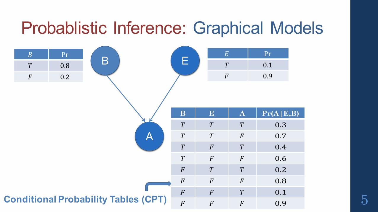
Probablistic Inference: Graphical Models
5
B E
A
B E A Pr(A|E,B)
Conditional Probability Tables (CPT)

6
B E
A
Pr 𝐸 ∩ 𝐴 =Pr 𝐸 ∗ Pr ¬𝐵 ∗ Pr 𝐴 𝐸, ¬𝐵
+ Pr 𝐸 ∗ Pr 𝐵 ∗ Pr 𝐴 𝐸, 𝐵]
Probabilistic Inference: First Principle Calculation
B E A Pr(A|E,B)

Probabilisitc Inference: Logical FormulationV = vA, v~A, vB, v~B, vE, v~E Prop vars corresponding to eventsT = tA|B,E , t~A|B,E , tA|B,~E … Prop vars corresponding to CPT entries
Formula encoding probabilistic graphical model (ϕPGM):(vA ⊕ v~A) ∧ (vB ⊕ v~B) ∧ (vE ⊕ v~E) Exactly one of vA and v~A is true
∧(tA|B,E ⇔ vA ∧ vB ∧ vE) ∧ (t~A|B,E ⇔ v~A ∧ vB ∧ vE) ∧ …
If vA , vB , vE are true, so must tA|B,E and vice versa
7

Probabilistic Inference: Logic and Weights
V = vA, v~A, vB, v~B, vE, v~ET = tA|B,E , t~A|B,E , tA|B,~E …
W(v~B) = 0.2, W(vB) = 0.8 Probabilities of indep events are weights of +ve literals
W(v~E) = 0.1, W(vE) = 0.9 W(tA|B,E) = 0.3, W(t~A|B,E) = 0.7, … CPT entries are weights of +ve literalsW(vA) = W(v~A) = 1 Weights of vars corresponding to dependent eventsW(¬v~B) = W(¬vB) = W(¬ tA|B,E) … = 1 Weights of -ve literals are all 1
Weight of assignment (vA = 1, v~A = 0, tA|B,E = 1, …) = W(vA) * W(¬v~A)* W( tA|B,E)* … Product of weights of literals in assignment 8

Probabilistic Inference: Discrete IntegrationV = vA, v~A, vB, v~B, vE, v~ET = tA|B,E , t~A|B,E , tA|B,~E …
Formula encoding combination of events in probabilistic model (Alarm and Earthquake) F = ϕPGM∧ vA ∧ vE
Set of satisfying assignments of F: RF = (vA = 1, vE = 1, vB = 1, tA|B,E = 1, all else 0), (vA = 1, vE = 1, v~B = 1, tA|~B,E = 1, all else 0)
Weight of satisfying assignments of F:W(RF) = W(vA) * W(vE) * W(vB) * W(tA|B,E ) + W(vA) * W(vE) * W(v~B) * W(tA|~B,E )
= 1* Pr[E] * Pr[B] * Pr[A | B,E] + 1* Pr[E] * Pr[~B] * Pr[A | ~B,E] = Pr[ A ∩ E] 9

Application 2: Network Reliability
Graph G = (V, E) represents a (power-grid) network • Nodes (V) are towns, villages, power stations• Edges (E) are power lines• Assume each edge e fails with prob g(e) ∈ [0,1] • Assume failure of edges statistically
independent• What is the probability that s and t become
disconnected?
10
st

Network Reliability: First Principles Modelingπ : E → 0, 1 … configuration of network
-- π(e) = 0 if edge e has failed, 1 otherwise
Prob of network being in configuration π
Pr[ π ] = Π g(e) × Π (1 - g(e))
Prob of s and t being disconnected
Pds,t = Σ Pr [π]
11
e: π(e) = 0 e: π(e) = 1
st
π : s, t disconnected in π
May need to sum over numerous (> 2100) configurations

Network Reliability: Discrete Integration• pv: Boolean variable for each v in V• qe: Boolean variable for each e in E
• ϕs,t (pv1, … pvn, qe1, … qem) : Boolean formula such that sat assignments σ of ϕs,t have 1-1 correspondence with configs π that disconnect s and t
- W(σ) = Pr[ π ]
12
st
Pds,t = Σ Pr [π] = Σ W(σ) = W(ϕ)
π : s, t disconnected in π 𝜎 ⊨ 𝜑𝑠, 𝑡

Application 3: Quantitative Information Flow• A password-checker PC takes a secret password (SP) and a user input (UI) and returns “Yes” iff SP = UI [Bang et al 2016] Suppose passwords are 4 characters (‘0’ through ‘9’) long
13
PC1 (char[] SP, char[] UI) for (int i=0; i<SP.length(); i++)
if(SP[i] != UI[i]) return “No”;return “Yes”;
PC2 (char[] H, char[] L) match = true;for (int i=0; i<SP.length(); i++)
if (SP[i] != UI[i]) match=false;else match = match;
if match return “Yes”;else return “No”;
Which of PC1 and PC2 is more likely to leak information about the secret key through side-channel observations?

QIF: Some Basics• Program P receives some “high” input (H) and produces a “low” (L) output Password checking: H is SP, L is time taken to answer “Is SP = UI?” Side-channel observations: memory, time …
• Adversary may infer partial information about H on seeing L E.g. in password checking, infer: 1st char is password is not 9.
• Can we quantify “leakage of information”?“initial uncertainty in H” = “info leaked” + “remaining uncertainty in H” [Smith 2009]
• Uncertainty and information leakage usually quantified using information theoretic measures, e.g. Shannon entropy
14

QIF: First Principles Approach• Password checking: Observed time to answer “Yes”/“No”
Depends on # instructions executed
• E.g. SP = 00700700UI = N2345678, 𝑁 ≠ 0
PC1 executes for loop onceUI = 02345678
PC1 executes for loop at least twiceObserving time to “No” gives away whether 1st char is not N, 𝑁 ≠ 0
In 10 attempts, 1st char can of SP can be uniquely determined.In max 40 attempts, SP can be cracked.
15
PC1 (char[] SP, char[] UI) for (int i=0; i<SP.length(); i++)
if(SP[i] != UI[i]) return “No”;return “Yes”;

QIF: First Principles Approach• Password checking: Observed time to answer “Yes”/“No” Depends on # instructions executed
• E.g. SP = 00700700
UI = N2345678, 𝑁 ≠ 0
PC1 executes for loop 4 times
UI = 02345678
PC1 executes for loop 4 times
Cracking SP requires max 104 attempts !!! (“less leakage”)16
PC2 (char[] H, char[] L) match = true;for (int i=0; i<SP.length(); i++)
if (SP[i] != UI[i]) match=false;else match = match;
if match return “Yes”;else return “No”;

QIF: Partitioning Space of Secret Password• Observable time effectively partitions values of SP [Bultan2016]
17
T
PC1 (char[] SP, char[] UI) for (int i=0; i<SP.length(); i++)
if(SP[i] != UI[i]) return “No”;return “Yes”;
SP[0] != UI[0]
“No”
F
SP[0] != UI[0]
t = 3
SP[1] != UI[1]
“No”
F
T
SP[1] != UI[1]SP[0] = UI[0]
t = 5
SP[2] != UI[2]
“No”
F
T
SP[2] != UI[2]SP[1] = UI[1]SP[0] = UI[0]
t = 7
SP[3] != UI[3]
“No”T
“Yes”
SP[3] = UI[3] SP[1] = UI[1]SP[2] = UI[2] SP[0] = UI[0]
F
SP[3] != UI[3]SP[2] = UI[2]SP[1] = UI[1]SP[0] = UI[0]
t = 9
t = 11

QIF: Probabilities of Observed Times
18
SP[0] != UI[0]
SP[1] != UI[1]
SP[2] != UI[2]
SP[3] != UI[3]
“No” “No” “No” “No”
F F F
T T T T
SP[0] != UI[0]
“Yes”
SP[3] = UI[3] SP[1] = UI[1]SP[2] = UI[2] SP[0] = UI[0]
F
SP[1] != UI[1]SP[0] = UI[0]
SP[2] != UI[2]SP[1] = UI[1]SP[0] = UI[0]
SP[3] != UI[3]SP[2] = UI[2]SP[1] = UI[1]SP[0] = UI[0]
t = 3 t = 5 t = 7 t = 9
t = 11
𝜑567 ∶ 𝑆𝑃 1 ≠ 𝑈𝐼 1 ∧ 𝑆𝑃 0 = 𝑈𝐼 0
Pr [ t = 5 ] = |@AB CDEF |GHI
Model Counting if UI
uniformly chosen

QIF: Probabilities of Observed Times
19
SP[0] != UI[0]
SP[1] != UI[1]
SP[2] != UI[2]
SP[3] != UI[3]
“No” “No” “No” “No”
F F F
T T T T
SP[0] != UI[0]
“Yes”
SP[3] = UI[3] SP[1] = UI[1]SP[2] = UI[2] SP[0] = UI[0]
F
SP[1] != UI[1]SP[0] = UI[0]
SP[2] != UI[2]SP[1] = UI[1]SP[0] = UI[0]
SP[3] != UI[3]SP[2] = UI[2]SP[1] = UI[1]SP[0] = UI[0]
t = 3 t = 5 t = 7 t = 9
t = 11
𝜑567 ∶ 𝑆𝑃 1 ≠ 𝑈𝐼 1 ∧ 𝑆𝑃 0 = 𝑈𝐼 0
Pr [ t = 5 ] = W(𝜑567) Discrete Integration if UI chosen according to
weight function

QIF: Quantifying Leakage via IntegrationExp information leakage =
Shannon entropy of obs times =
Information leakage in password checker example PC1: 0.52 (more “leaky”)PC2: 0.0014 (less “leaky”)
Discrete integration crucial in obtaining Pr[t = k]
20
K Pr 𝑡 = 𝑘 . log1/Pr[𝑡 = 𝑘]S∈V,7,W,X,GG

Unweighted Counting Suffices in Principle
Weighted Model Counting
21
Weighted Model Counting Unweighted Model Counting
Reduction polynomial in #bits representing weightsIJCAI 2015
Probabilistic Inference
Network Reliability
Quantified Information Flow
DMPV 2017
KML 1989, Karger 2000

Application 4: Constr Random Verification
Functional Verification• Formal verificationChallenges: formal requirements, scalability~10-15% of verification effort
• Dynamic verification: dominant approach
22

CRV: Dynamic Verification
§Design is simulated with test vectors• Test vectors represent different verification scenarios §Results from simulation compared to intended results
§How do we generate test vectors?Challenge: Exceedingly large test input space!
Can’t try all input combinations2128 combinations for a 64-bit binary operator!!!
23

CRV: Sources of Constraints
24§ Test vectors: solutions of constraints
§ Proposed by Lichtenstein, Malka, Aharon (IAAI 94)
a b
c
64 bit
64 bit
64 bit
c = f(a,b)
• Designers: 1. a +64 11 *32 b = 122. a <64 (b >> 4)
• Past Experience: 1. 40 <64 34 + a <64 50502. 120 <64 b <64 230
• Users:1. 232 *32 a + b != 11002. 1020 <64 (b /64 2) +64 a <64 2200

CRV: Why Existing Solvers Don’t Suffice
25
a b
c
64 bit
64 bit
64 bit
c = f(a,b)
Constraints• Designers:
1. a +64 11 *32 b = 122. a <64 (b >> 4)
• Past Experience: 1. 40 <64 34 + a <64 50502. 120 <64 b <64 230
• Users:1. 232 *32 a + b != 11002. 1020 <64 (b /64 2) +64 a <64 2200
Modern SAT/SMT solvers are complex systemsEfficiency stems from the solver automatically “biasing” searchFails to give unbiased or user-biased distribution of test vectors

CRV: Need To Go Beyond SAT Solvers
26
Set of Constraints
Sample satisfying assignments uniformly at random
SAT Formula
Scalable Uniform Generation of SAT Witnesses
a b
c
64 bit
64 bit
64 bit
c = f(a,b)
Constrained Random Verification

Application 5: Automated Problem Generation• Large class sizes, MOOC offerings require automated generation of related but randomly different problems
• Discourages plagiarism between students
• Randomness makes it hard for students to guess what the solution would be
• Allows instructors to focus on broad parameters of problems, rather than on individual problem instances
• Enables development of automated intelligent tutoring systems
27

Auto Prob Gen: Using Problem Templates• A problem template is a partial specification of a problem
“Holes” in the template must be filled with elements from specified sets Constraints on elements chosen to fill various “holes” restricts problem
instances so that undesired instances are eliminated
• Example: Non-deterministic finite automata to be generated for complementation
Holes: States, alphabet size, transitions for (state, letter) pairs, final states, initial states
Constraints: Alphabet size = 2Min/max transitions for a (state, letter) pair = 0/4Min/max states = 3/5Min/max number of final states = 1/3Min/max initial states = 1/2
28

Auto Prob Gen: An Illustration Non-det finite automaton encoded as a formula on following variables
s1, s2, s3, s4, s5 : States f1, f2, f3, f4, f5: Final statesn1, n2, n3, n4, n5: Initial statess1a1s2, s1a2s2, … : Transitions
𝜑 Z[Z5 = \ 𝑛Z → 𝑠Z ∧ 1 ≤K𝑛ZZ
≤ 2Z
𝜑 5ab[c = \ 𝑠Z𝑎e𝑠S → 𝑠Z ∧ 𝑠S ∧\ 0 ≤K𝑠Z𝑎e𝑠S ≤ 4SZ,eZ
𝜑 c5gAh[5 = 3 ≤ ∑ 𝑠ZZ ≤ 5
𝜑 lZ[c5 =\ 𝑓Z → 𝑠Z ∧ 1 ≤ K𝑓ZZ
≤ 3 Z
29
Every solution of 𝜑 Z[Z5 ∧ 𝜑 5ab[c∧ 𝜑 c5gAh[5 ∧ 𝜑 lZ[c5gives an automaton satisfying specified
constraints

Auto Prob Gen: An Illustration Non-det finite automaton encoded as a formula on following variables
s1 = 1, s2 = 0, s3 = 1, s4 = 1, s5 = 1: States f1 = 0, f2 = 0, f3 = 1, f4 = 1, f5 = 0: Final statesn1 = 1, n2 = 0, n3 = 0, n4 = 0, n5 = 0: Initial statess1a1s3 = 1, s1a1s4 = 1, s4a2s4 = 1, s4a1s5 = 1, … : Transitions
30
s1
s3
s4
s5
a1
a1a1
a5

Auto Prob Gen: Discrete Sampling• Uniform random generation of solutions of constraints gives automata satisfying constraints randomly
• Weighted random generation of solutions gives automata satisfying constraints with different priorities/weightages.
Examples: Weighing final state variables more gives automata with more final statesWeighing transitions on letter a1 more gives automatawith more transitions labeled a1
31

Discrete Sampling and Integration
for the AI Practitioner
Supratik Chakraborty, IIT Bombay
Kuldeep S. Meel, Rice UniversityMoshe Y. Vardi, Rice University
Part 2b: Survey of Prior Work

How Hard is it to Count/Sample? • Trivial if we could enumerate RF: Almost always impractical
• Computational complexity of counting (discrete integration):
Exact unweighted counting: #P-complete [Valiant 1978]
Approximate unweighted counting:
Deterministic: Polynomial time det. Turing Machine with Σ2p oracle [Stockmeyer 1983]
Randomized: Poly-time probabilistic Turing Machine with NP oracle
[Stockmeyer 1983; Jerrum,Valiant,Vazirani 1986]
Probably Approximately Correct (PAC) algorithm
Weighted versions of counting: Exact: #P-complete [Roth 1996],
Approximate: same class as unweighted version [follows from Roth 1996] 33
0for ),1(||) e(F,DetEstimat 1
|| >+×≤≤+
εεεε FF RR
10,0for ,1)1(||), te(F,RandEstima1
||Pr ≤<>−≥⎥⎦⎤
⎢⎣⎡ +⋅≤≤+
δεδεδεε FF RR
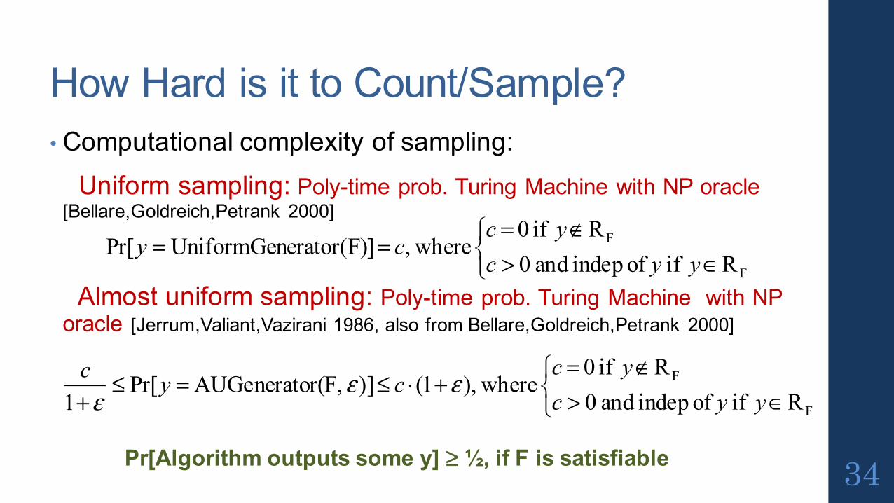
How Hard is it to Count/Sample?• Computational complexity of sampling:
Uniform sampling: Poly-time prob. Turing Machine with NP oracle [Bellare,Goldreich,Petrank 2000]
Almost uniform sampling: Poly-time prob. Turing Machine with NP oracle [Jerrum,Valiant,Vazirani 1986, also from Bellare,Goldreich,Petrank 2000]
34
R if of indep and0
R if 0 where, erator(F)]UniformGenPr[
F
F
⎩⎨⎧
∈>∉=
==y yc
yccy
⎩⎨⎧
∈>∉=
+⋅≤=≤+ F
F
R if of indep and0R if 0
where,)1( )] r(F,AUGeneratoPr[1 y yc
yccyc εε
ε
Pr[Algorithm outputs some y] ≥ ½, if F is satisfiable

Markov Chain Monte Carlo Techniques• Rich body of theoretical work with applications to sampling and counting
[Jerrum,Sinclair 1996]• Some popular (and intensively studied) algorithms:
Metropolis-Hastings [Metropolis et al 1953, Hastings 1970], Simulated Annealing [Kirkpatrick et al 1982]
• High-level idea: Start from a “state” (assignment of variables) Randomly choose next state using “local” biasing functions (depends on target
distribution & algorithm parameters) Repeat for an appropriately large number (N) of steps After N steps, samples follow target distribution with high confidence
• Convergence to desired distribution guaranteed only after N (large) steps• In practice, steps truncated early heuristically
Nullifies/weakens theoretical guarantees [Kitchen,Keuhlman 2007]35

Exact Counters• DPLL based counters [CDP: Birnbaum,Lozinski 1999] DPLL branching search procedure, with partial truth assignments Once a branch is found satisfiable, if t out of n variables assigned, add
2n-t to model count, backtrack to last decision point, flip decision and continue
Requires data structure to check if all clauses are satisfied by partial assignment
Usually not implemented in modern DPLL SAT solvers Can output a lower bound at any time
36

Exact Counters• DPLL + component analysis [RelSat: Bayardo, Pehoushek 2000] Constraint graph G:
Variables of F are verticesAn edge connects two vertices if corresponding variables appear in some clause of F
Disjoint components of G lazily identified during DPLL search F1, F2, … Fn : subformulas of F corresponding to components
|RF| = |RF1| * |RF2| * |RF3| * … Heuristic optimizations:
Solve most constrained sub-problems firstSolving sub-problems in interleaved manner
37

Exact Counters• DPLL + Caching [Bacchus et al 2003, Cachet: Sang et al 2004,
sharpSAT: Thurley 2006]If same sub-formula revisited multiple times during DPLL search, cache result and re-use it“Signature” of the satisfiable sub-formula/component must be storedDifferent forms of caching used:
Simple sub-formula cachingComponent cachingLinear-space caching
Component caching can also be combined with clause learning and other reasoning techniques at each node of DPLL search tree
WeightedCachet: DPLL + Caching for weighted assignments 38
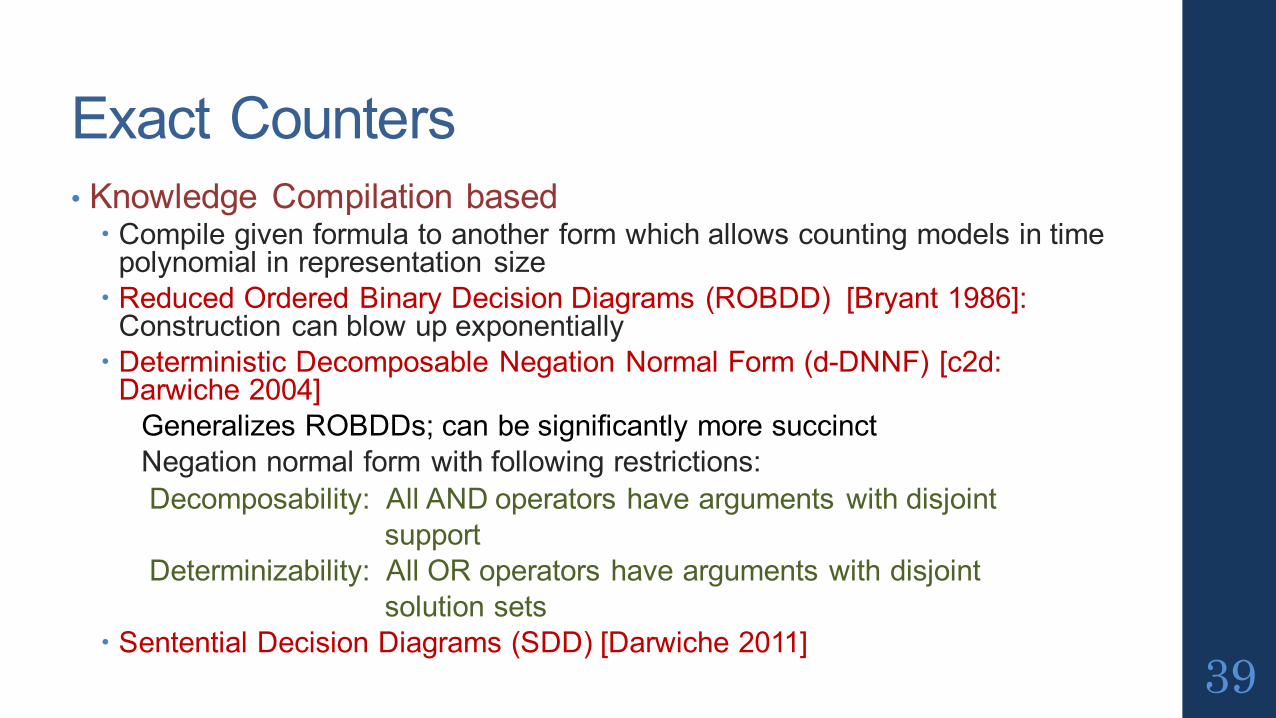
Exact Counters• Knowledge Compilation based
Compile given formula to another form which allows counting models in time polynomial in representation size
Reduced Ordered Binary Decision Diagrams (ROBDD) [Bryant 1986]: Construction can blow up exponentially
Deterministic Decomposable Negation Normal Form (d-DNNF) [c2d: Darwiche 2004]
Generalizes ROBDDs; can be significantly more succinctNegation normal form with following restrictions:Decomposability: All AND operators have arguments with disjoint
supportDeterminizability: All OR operators have arguments with disjoint
solution sets Sentential Decision Diagrams (SDD) [Darwiche 2011]
39

Exact Counters: How far do they go?• Work reasonably well in small-medium sized problems, and in large problem instances with special structure
• Use them whenever possible #P-completeness hits back eventually – scalability suffers!
40

Bounding Counters[MBound: Gomes et al 2006; SampleCount: Gomes et al 2007; BPCount: Kroc et al 2008]
Provide lower and/or upper bounds of model count Usually more efficient than exact counters No approximation guarantees on bounds
Useful only for limited applications
41
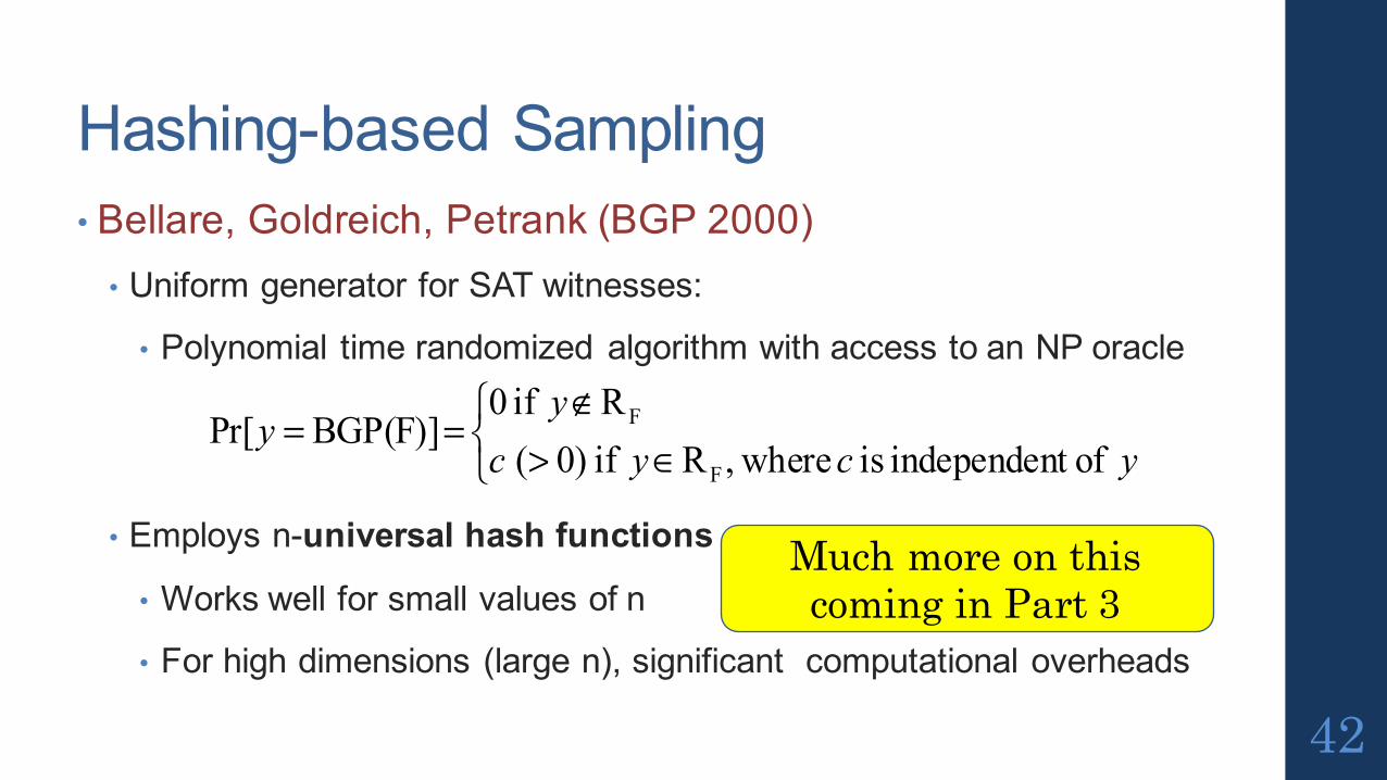
Hashing-based Sampling• Bellare, Goldreich, Petrank (BGP 2000)
• Uniform generator for SAT witnesses:
• Polynomial time randomized algorithm with access to an NP oracle
• Employs n-universal hash functions
• Works well for small values of n
• For high dimensions (large n), significant computational overheads
42
⎩⎨⎧
∈>∉
==ycyc
yy
oft independen is where,R if)0(R if 0
BGP(F)]Pr[F
F
Much more on this coming in Part 3

Approximate Integration and Sampling: Close Cousins
Almost-Uniform Generator
PAC Counter
Polynomial
reduction
• Yet, no practical algorithms that scale to large problem instances were derived from this work
• No scalable PAC counter or almost-uniform generator existed until a few years back
• The inter-reductions are practically computation intensive•Think of O(n) calls to the counter when n = 100000 43
• Seminal paper by Jerrum, Valiant, Vazirani 1986

Prior Work
44Performance
Gua
rant
ees
MCMC
SAT-Based
BGP
BDD/other exact tech.

Techniques using XOR hash functions• Bounding counters MBound, SampleCount [Gomes et al. 2006, Gomes et al 2007] used random XORs Algorithms geared towards finding bounds without approximation
guarantees Power of 2-universal hashing not exploited
• In a series of papers [2013: ICML, UAI, NIPS; 2014: ICML; 2015: ICML, UAI; 2016: AAAI, ICML, AISTATS, …] Ermon et al used XOR hash functions for discrete counting/sampling Random XORs, also XOR constraints with specific structures 2-universality exploited to provide improved guarantees Relaxed constraints (like short XORs) and their effects studied
45

An Interesting Combination: XOR + MAP Optimization• WISH: Ermon et al 2013• Given a weight function W: 0,1n → ℜ≥0
Use random XORs to partition solutions into cells After partitioning into 2, 4, 8, 16, … cells
Use Max Aposteriori Probability (MAP) optimizer to find solution with max weight in a cell (say, a2, a4, a8, a16, …)
Estimated W(RF) = W(a2)*1 + W(a4)*2 + W(a8)* 4 + …
• Constant factor approximation of W(RF) with high confidence• MAP oracle needs repeated invokation O(n.log2n)
MAP is NP-complete Being optimization (not decision) problem), MAP is harder to solve in
practice than SAT
46

XOR-based Counting and Sampling• Remainder of tutorial Deeper dive into XOR hash-based counting and sampling Discuss theoretical aspects and experimental observations
Based on work published in [2013: CP, CAV; 2014: DAC, AAAI; 2015: IJCAI, TACAS; 2016: AAAI, IJCAI, 2017: AAAI]
47

Discrete Sampling and Integration for the AIPractitioner
Part III: Hashing-based Approach to Sampling andIntegration
Supratik Chakraborty, IIT BombayKuldeep S. Meel, Rice UniversityMoshe Y. Vardi, Rice University
1 / 41

Discrete Integration and Sampling
• Given
– Variables X1,X2, · · ·Xn over finite discrete domains D1,D2, · · ·Dn
– Formula ϕ over X1,X2, · · ·Xn
– Weight Function W : D1 × D2 · · · × Dn 7→ [0, 1]
• Sol(ϕ) = solutions of F
• Discrete Integration: Determine W (ϕ) = Σy∈Sol(ϕ)W (y)
– If W (y) = 1 for all y , then W (ϕ) = |Sol(ϕ)|
• Discrete Sampling: Randomly sample from Sol(ϕ) such thatPr[y is sampled] ∝W (y)
– If W (y) = 1 for all y , then uniformly sample from Sol(ϕ)
2 / 41

Part I
Discrete Integration
3 / 41

From Weighted to Unweighted Integration
Boolean Formula ϕ and weightfunction W : 0, 1n → Q≥0
4 / 41

From Weighted to Unweighted Integration
Boolean Formula ϕ and weightfunction W : 0, 1n → Q≥0 Boolean Formula F ′
W (ϕ) = c(W )× |Sol(F ′)|
4 / 41

From Weighted to Unweighted Integration
Boolean Formula ϕ and weightfunction W : 0, 1n → Q≥0 Boolean Formula F ′
W (ϕ) = c(W )× |Sol(F ′)|
• Key Idea: Encode weight function as a set of constraints
(CFMV, IJCAI15)
4 / 41

From Weighted to Unweighted Integration
Boolean Formula ϕ and weightfunction W : 0, 1n → Q≥0 Boolean Formula F ′
W (ϕ) = c(W )× |Sol(F ′)|
• Key Idea: Encode weight function as a set of constraints
(CFMV, IJCAI15)
How do we estimate |Sol(F ′)|?
4 / 41

As Simple as Counting Dots

As Simple as Counting Dots

As Simple as Counting Dots
Pick a random cell
Estimate = Number of solutions in a cell × Number of cells
5 / 41

Challenges
Challenge 1 How to partition into roughly equal small cells of solutionswithout knowing the distribution of solutions?
6 / 41

Challenges
Challenge 1 How to partition into roughly equal small cells of solutionswithout knowing the distribution of solutions?
Challenge 2 How large is a “small” cell?
6 / 41

Challenges
Challenge 1 How to partition into roughly equal small cells of solutionswithout knowing the distribution of solutions?
Challenge 2 How large is a “small” cell?
Challenge 3 How many cells?
6 / 41

Challenges
Challenge 1 How to partition into roughly equal small cells of solutionswithout knowing the distribution of solutions?
• Designing function h : assignments → cells (hashing)• Solutions in a cell α: Sol(ϕ) ∩ y | h(y) = α
6 / 41

Challenges
Challenge 1 How to partition into roughly equal small cells of solutionswithout knowing the distribution of solutions?
• Designing function h : assignments → cells (hashing)• Solutions in a cell α: Sol(ϕ) ∩ y | h(y) = α• Deterministic h unlikely to work
6 / 41

Challenges
Challenge 1 How to partition into roughly equal small cells of solutionswithout knowing the distribution of solutions?
• Designing function h : assignments → cells (hashing)• Solutions in a cell α: Sol(ϕ) ∩ y | h(y) = α• Deterministic h unlikely to work• Choose h randomly from a large family H of hashfunctionsUniversal Hashing (Carter and Wegman 1977)
6 / 41

r-Universal Hashing
• Let H be family of r−universal hash functions mapping 0, 1n to0, 1m
∀y1, y2, · · · yr ∈ 0, 1n, α1, α2, · · ·αr ∈ 0, 1
m, hR←− H
Pr[h(y1) = α1] = · · ·Pr[h(yr ) = αr ] =
(
1
2m
)
Pr[h(y1) = α1 ∧ · · · ∧ h(yr ) = αr ] =
(
1
2m
)r
7 / 41

Desired Properties
• Let h be randomly picked a family of hash function H and Z bethe number of solutions in a randomly chosen cell α
– What is E[Z ] and how much does Z deviate from E[Z ]?
• For every y ∈ Sol(ϕ), we define Iy =
1 h(y) = α(y is in cell)
0 otherwise
• Z =∑
y∈Sol(ϕ) Iy
– Desired: E[Z ] = |Sol(ϕ)|2m and σ2[Z ] ≤ E[Z ]
8 / 41

Desired Properties
• Let h be randomly picked a family of hash function H and Z bethe number of solutions in a randomly chosen cell α
– What is E[Z ] and how much does Z deviate from E[Z ]?
• For every y ∈ Sol(ϕ), we define Iy =
1 h(y) = α(y is in cell)
0 otherwise
• Z =∑
y∈Sol(ϕ) Iy
– Desired: E[Z ] = |Sol(ϕ)|2m and σ2[Z ] ≤ E[Z ]
– It suffices to have H to be 2-universal
8 / 41

Desired Properties
• Let h be randomly picked a family of hash function H and Z bethe number of solutions in a randomly chosen cell α
– What is E[Z ] and how much does Z deviate from E[Z ]?
• For every y ∈ Sol(ϕ), we define Iy =
1 h(y) = α(y is in cell)
0 otherwise
• Z =∑
y∈Sol(ϕ) Iy
– Desired: E[Z ] = |Sol(ϕ)|2m and σ2[Z ] ≤ E[Z ]
– It suffices to have H to be 2-universal– Pr
[
E[Z ]1+ε≤ Z ≤ E[Z ](1 + ε)
]
≥ 1− σ2[Z ]
( ε
1+ε)2(E[Z ])2
8 / 41

Desired Properties
• Let h be randomly picked a family of hash function H and Z bethe number of solutions in a randomly chosen cell α
– What is E[Z ] and how much does Z deviate from E[Z ]?
• For every y ∈ Sol(ϕ), we define Iy =
1 h(y) = α(y is in cell)
0 otherwise
• Z =∑
y∈Sol(ϕ) Iy
– Desired: E[Z ] = |Sol(ϕ)|2m and σ2[Z ] ≤ E[Z ]
– It suffices to have H to be 2-universal– Pr
[
E[Z ]1+ε≤ Z ≤ E[Z ](1 + ε)
]
≥ 1− σ2[Z ]
( ε
1+ε)2(E[Z ])2 ≥ 1− 1
( ε
1+ε)2(E[Z ])
8 / 41

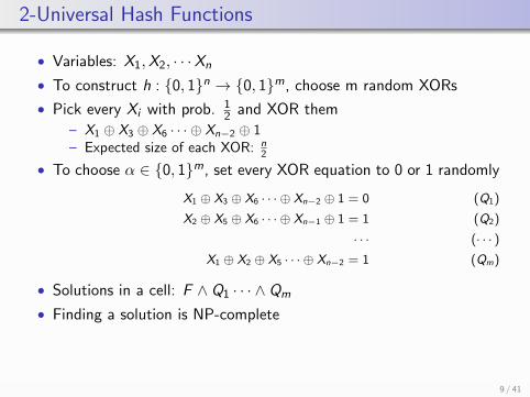
2-Universal Hash Functions
• Variables: X1,X2, · · ·Xn
• To construct h : 0, 1n → 0, 1m, choose m random XORs
• Pick every Xi with prob. 12 and XOR them
– X1 ⊕ X3 ⊕ X6 · · · ⊕ Xn−2 ⊕ 1– Expected size of each XOR: n
2
9 / 41

2-Universal Hash Functions
• Variables: X1,X2, · · ·Xn
• To construct h : 0, 1n → 0, 1m, choose m random XORs
• Pick every Xi with prob. 12 and XOR them
– X1 ⊕ X3 ⊕ X6 · · · ⊕ Xn−2 ⊕ 1– Expected size of each XOR: n
2
• To choose α ∈ 0, 1m, set every XOR equation to 0 or 1 randomly
X1 ⊕ X3 ⊕ X6 · · · ⊕ Xn−2 ⊕ 1 = 0 (Q1)
X2 ⊕ X5 ⊕ X6 · · · ⊕ Xn−1 ⊕ 1 = 1 (Q2)
· · · (· · · )
X1 ⊕ X2 ⊕ X5 · · · ⊕ Xn−2 = 1 (Qm)
• Solutions in a cell: F ∧ Q1 · · · ∧ Qm
9 / 41
2-Universal Hash Functions
• Variables: X1,X2, · · ·Xn
• To construct h : 0, 1n → 0, 1m, choose m random XORs
• Pick every Xi with prob. 12 and XOR them
– X1 ⊕ X3 ⊕ X6 · · · ⊕ Xn−2 ⊕ 1– Expected size of each XOR: n
2
• To choose α ∈ 0, 1m, set every XOR equation to 0 or 1 randomly
X1 ⊕ X3 ⊕ X6 · · · ⊕ Xn−2 ⊕ 1 = 0 (Q1)
X2 ⊕ X5 ⊕ X6 · · · ⊕ Xn−1 ⊕ 1 = 1 (Q2)
· · · (· · · )
X1 ⊕ X2 ⊕ X5 · · · ⊕ Xn−2 = 1 (Qm)
• Solutions in a cell: F ∧ Q1 · · · ∧ Qm
• Finding a solution is NP-complete
9 / 41

2-Universal Hash Functions
• Variables: X1,X2, · · ·Xn
• To construct h : 0, 1n → 0, 1m, choose m random XORs• Pick every Xi with prob. 1
2 and XOR them– X1 ⊕ X3 ⊕ X6 · · · ⊕ Xn−2 ⊕ 1– Expected size of each XOR: n
2• To choose α ∈ 0, 1m, set every XOR equation to 0 or 1 randomly
X1 ⊕ X3 ⊕ X6 · · · ⊕ Xn−2 ⊕ 1 = 0 (Q1)
X2 ⊕ X5 ⊕ X6 · · · ⊕ Xn−1 ⊕ 1 = 1 (Q2)
· · · (· · · )
X1 ⊕ X2 ⊕ X5 · · · ⊕ Xn−2 = 1 (Qm)
• Solutions in a cell: F ∧ Q1 · · · ∧ Qm
• Finding a solution is NP-completeModern SAT solvers are able to deal routinely with practicalproblems that involve many thousands of variables, although suchproblems were regarded as hopeless just a few years ago.
(Knuth, 2016)
9 / 41

2-Universal Hash Functions
• Variables: X1,X2, · · ·Xn
• To construct h : 0, 1n → 0, 1m, choose m random XORs
• Pick every Xi with prob. 12 and XOR them
– X1 ⊕ X3 ⊕ X6 · · · ⊕ Xn−2 ⊕ 1– Expected size of each XOR: n
2
• To choose α ∈ 0, 1m, set every XOR equation to 0 or 1 randomly
X1 ⊕ X3 ⊕ X6 · · · ⊕ Xn−2 ⊕ 1 = 0 (Q1)
X2 ⊕ X5 ⊕ X6 · · · ⊕ Xn−1 ⊕ 1 = 1 (Q2)
· · · (· · · )
X1 ⊕ X2 ⊕ X5 · · · ⊕ Xn−2 = 1 (Qm)
• Solutions in a cell: F ∧ Q1 · · · ∧ Qm
• Finding a solution is NP-complete
• Performance of state of the art SAT solvers degrade with increasein the size of XORs (SAT Solvers != SAT oracles)
9 / 41

Improved Universal Hash Functions
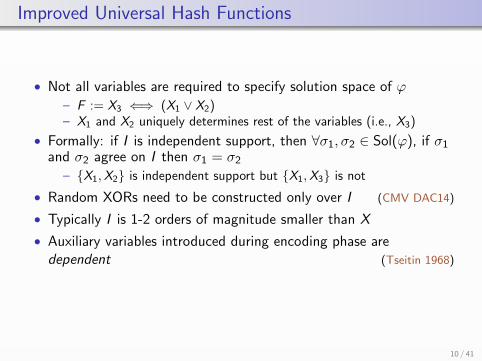
• Not all variables are required to specify solution space of ϕ
– F := X3 ⇐⇒ (X1 ∨ X2)– X1 and X2 uniquely determines rest of the variables (i.e., X3)
• Formally: if I is independent support, then ∀σ1, σ2 ∈ Sol(ϕ), if σ1and σ2 agree on I then σ1 = σ2
– X1,X2 is independent support but X1,X3 is not
10 / 41

Improved Universal Hash Functions
• Not all variables are required to specify solution space of ϕ
– F := X3 ⇐⇒ (X1 ∨ X2)– X1 and X2 uniquely determines rest of the variables (i.e., X3)
• Formally: if I is independent support, then ∀σ1, σ2 ∈ Sol(ϕ), if σ1and σ2 agree on I then σ1 = σ2
– X1,X2 is independent support but X1,X3 is not
• Random XORs need to be constructed only over I (CMV DAC14)
10 / 41
Improved Universal Hash Functions
• Not all variables are required to specify solution space of ϕ
– F := X3 ⇐⇒ (X1 ∨ X2)– X1 and X2 uniquely determines rest of the variables (i.e., X3)
• Formally: if I is independent support, then ∀σ1, σ2 ∈ Sol(ϕ), if σ1and σ2 agree on I then σ1 = σ2
– X1,X2 is independent support but X1,X3 is not
• Random XORs need to be constructed only over I (CMV DAC14)
• Typically I is 1-2 orders of magnitude smaller than X
• Auxiliary variables introduced during encoding phase aredependent (Tseitin 1968)
10 / 41

Improved Universal Hash Functions
• Not all variables are required to specify solution space of ϕ
– F := X3 ⇐⇒ (X1 ∨ X2)– X1 and X2 uniquely determines rest of the variables (i.e., X3)
• Formally: if I is independent support, then ∀σ1, σ2 ∈ Sol(ϕ), if σ1and σ2 agree on I then σ1 = σ2
– X1,X2 is independent support but X1,X3 is not
• Random XORs need to be constructed only over I (CMV DAC14)
• Typically I is 1-2 orders of magnitude smaller than X
• Auxiliary variables introduced during encoding phase aredependent (Tseitin 1968)
Algorithmic procedure to determine I?
10 / 41

Independent Support
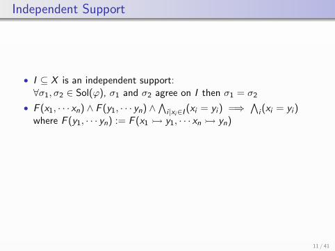
• I ⊆ X is an independent support:∀σ1, σ2 ∈ Sol(ϕ), σ1 and σ2 agree on I then σ1 = σ2
11 / 41
Independent Support
• I ⊆ X is an independent support:∀σ1, σ2 ∈ Sol(ϕ), σ1 and σ2 agree on I then σ1 = σ2
• F (x1, · · · xn) ∧ F (y1, · · · yn) ∧∧
i |xi∈I(xi = yi ) =⇒
∧
i (xi = yi )where F (y1, · · · yn) := F (x1 y1, · · · xn yn)
11 / 41

Independent Support
• I ⊆ X is an independent support:∀σ1, σ2 ∈ Sol(ϕ), σ1 and σ2 agree on I then σ1 = σ2
• F (x1, · · · xn) ∧ F (y1, · · · yn) ∧∧
i |xi∈I(xi = yi ) =⇒
∧
i (xi = yi )where F (y1, · · · yn) := F (x1 y1, · · · xn yn)
• QF ,I := F (x1, · · · xn) ∧ F (y1, · · · yn) ∧∧
i |xi∈I(xi = yi ) ∧ ¬(
∧
i (xi =yi ))
• Lemma: QF ,I is UNSAT if and only if I is independent support
11 / 41

Independent Support
H1 := x1 = y1,H2 := x2 = y2, · · ·Hn := xn = yn
Ω = F (x1, · · · xn) ∧ F (y1, · · · yn) ∧ ¬(∧
i
(xi = yi ))
Lemma
I = xi is independent support iif HI ∧ Ω is UNSAT where
H I = Hi |xi ∈ I
12 / 41

Minimal Unsatisfiable Subset
Given Ψ = H1 ∧ H2 · · · ∧ Hm ∧ Ω
Unsatisfiable Subset Find subset Hi1,Hi2, · · ·Hik of H1,H2, · · ·Hmsuch that Hi1 ∧ Hi2 ∧ Hik ∧ Ω is UNSAT
13 / 41

Minimal Unsatisfiable Subset
Given Ψ = H1 ∧ H2 · · · ∧ Hm ∧ Ω
Unsatisfiable Subset Find subset Hi1,Hi2, · · ·Hik of H1,H2, · · ·Hmsuch that Hi1 ∧ Hi2 ∧ Hik ∧ Ω is UNSAT
Minimal Unsatisfiable Subset Find minimal subset Hi1,Hi2, · · ·Hikof H1,H2, · · ·Hm such that Hi1 ∧ Hi2 ∧ Hik ∧ Ω isUNSAT
13 / 41

Minimal Unsatisfiable Subset
Given Ψ = H1 ∧ H2 · · · ∧ Hm ∧ Ω
Unsatisfiable Subset Find subset Hi1,Hi2, · · ·Hik of H1,H2, · · ·Hmsuch that Hi1 ∧ Hi2 ∧ Hik ∧ Ω is UNSAT
Minimal Unsatisfiable Subset Find minimal subset Hi1,Hi2, · · ·Hikof H1,H2, · · ·Hm such that Hi1 ∧ Hi2 ∧ Hik ∧ Ω isUNSAT
13 / 41

Minimal Independent Support
H1 := x1 = y1,H2 := x2 = y2, · · ·Hn := xn = yn
Ω = F (x1, · · · xn) ∧ F (y1, · · · yn) ∧ ¬(∧
i
(xi = yi ))
Lemma
I = xi is Minimal Independent Support iif H I is Minimal UnsatisfiableSubset where H I = Hi |xi ∈ I
MIS MUS
14 / 41

Minimal Independent Support
H1 := x1 = y1,H2 := x2 = y2, · · ·Hn := xn = yn
Ω = F (x1, · · · xn) ∧ F (y1, · · · yn) ∧ ¬(∧
i
(xi = yi ))
Lemma
I = xi is Minimal Independent Support iif H I is Minimal UnsatisfiableSubset where H I = Hi |xi ∈ I
MIS MUSTwo orders of magnitude improvement in runtime
14 / 41

Challenges
Challenge 1 How to partition into roughly equal small cells of solutionswithout knowing the distribution of solutions?
• Independent Support-based 2-Universal HashFunctions
Challenge 2 How large is a “small” cell?
Challenge 3 How many cells?
15 / 41

Challenge 2: How large is a “small” cell
• Too large Hard to enumerate
16 / 41

Challenge 2: How large is a “small” cell
• Too large Hard to enumerate
• Too small Weaker probabilistic guarantees
16 / 41

Challenge 2: How large is a “small” cell
• Too large Hard to enumerate
• Too small Weaker probabilistic guarantees
– Pr[
E[Z ]1+ε≤ Z ≤ E[Z ](1 + ε)
]
≥ 1− 1( ε
1+ε)2(E[Z ])
16 / 41

Challenge 2: How large is a “small” cell
• Too large Hard to enumerate
• Too small Weaker probabilistic guarantees
– Pr[
E[Z ]1+ε≤ Z ≤ E[Z ](1 + ε)
]
≥ 1− 1( ε
1+ε)2(E[Z ])
We want a “small” cell to have roughly thresh solutions, wherethresh = 5
(
1 + 1ε2
)
16 / 41

Challenges
Challenge 1 How to partition into roughly equal small cells of solutionswithout knowing the distribution of solutions?
• Independent Support-based 2-Universal HashFunctions
Challenge 2 How large is a “small” cell?
• Independent Support-based 2-Universal HashFunctions
Challenge 3 How many cells?
17 / 41

Challenge 3: How many cells?
• A cell is small if it has less than thresh = 5(1 + 1ε)2 solutions
• We want to partition into 2m∗
cells such that 2m∗
= |Sol(ϕ)|thresh
18 / 41

Challenge 3: How many cells?
• A cell is small if it has less than thresh = 5(1 + 1ε)2 solutions
• We want to partition into 2m∗
cells such that 2m∗
= |Sol(ϕ)|thresh
– Check for every m = 0, 1, · · · n if the number of solutions ≤ thresh
18 / 41

Challenge 3: How many cells?
• A cell is small if it has less than thresh = 5(1 + 1ε)2 solutions
• We want to partition into 2m∗
cells such that 2m∗
= |Sol(ϕ)|thresh
– Check for every m = 0, 1, · · · n if the number of solutions ≤ thresh– XORs for each m must be independently chosen
18 / 41

Challenge 3: How many cells?
• A cell is small if it has less than thresh = 5(1 + 1ε)2 solutions
• We want to partition into 2m∗
cells such that 2m∗
= |Sol(ϕ)|thresh
– Check for every m = 0, 1, · · · n if the number of solutions ≤ thresh– XORs for each m must be independently chosen
Query 1: Is #(F ∧ Q11 ) ≤ thresh
Query 2: Is #(F ∧ Q21 ∧ Q2
2 ) ≤ thresh
· · ·
Query n: Is #(F ∧ Qn1 · · · ∧ Qn
n ) ≤ thresh
– Stop at the first m where Query m returns YES and return estimateas #(F ∧ Qm
1 · · · ∧ Qmm )× 2m
• Number of SAT calls is O(n) (CMV, CP13) (CFMSV, AAAI14)
18 / 41

ApproxMC(F , ε, δ)
# of sols≤ thresh?
19 / 41

ApproxMC(F , ε, δ)
# of sols≤ thresh?
# of sols≤ thresh?
No
19 / 41

ApproxMC(F , ε, δ)
# of sols≤ thresh?
# of sols≤ thresh?
No No
19 / 41

ApproxMC(F , ε, δ)
# of sols≤ thresh?
# of sols≤ thresh?
# of sols≤ thresh?
# of sols≤ thresh?
· · ·
No No
No
19 / 41

ApproxMC(F , ε, δ)
# of sols≤ thresh?
# of sols≤ thresh?
# of sols≤ thresh?
Estimate =# of sols ×# of cells # of sols
≤ thresh?
· · ·
No No
No
Yes
19 / 41

ApproxMC(F , ε, δ)
Theoretical Guarantees
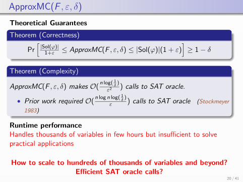
Theorem (Correctness)
Pr[
|Sol(ϕ)|1+ε
≤ ApproxMC(F , ε, δ) ≤ |Sol(ϕ)|(1 + ε)]
≥ 1− δ
Theorem (Complexity)
ApproxMC(F , ε, δ) makes O(n log( 1
δ)
ε2) calls to SAT oracle.
• Prior work required O(n log n log( 1
δ)
ε) calls to SAT oracle (Stockmeyer
1983)
20 / 41

ApproxMC(F , ε, δ)
Theoretical Guarantees
Theorem (Correctness)
Pr[
|Sol(ϕ)|1+ε
≤ ApproxMC(F , ε, δ) ≤ |Sol(ϕ)|(1 + ε)]
≥ 1− δ
Theorem (Complexity)
ApproxMC(F , ε, δ) makes O(n log( 1
δ)
ε2) calls to SAT oracle.
• Prior work required O(n log n log( 1
δ)
ε) calls to SAT oracle (Stockmeyer
1983)
Runtime performance
20 / 41

ApproxMC(F , ε, δ)
Theoretical Guarantees
Theorem (Correctness)
Pr[
|Sol(ϕ)|1+ε
≤ ApproxMC(F , ε, δ) ≤ |Sol(ϕ)|(1 + ε)]
≥ 1− δ
Theorem (Complexity)
ApproxMC(F , ε, δ) makes O(n log( 1
δ)
ε2) calls to SAT oracle.
• Prior work required O(n log n log( 1
δ)
ε) calls to SAT oracle (Stockmeyer
1983)
Runtime performanceHandles thousands of variables in few hours but insufficient to solvepractical applications
How to scale to hundreds of thousands of variables and beyond?
20 / 41
ApproxMC(F , ε, δ)
Theoretical Guarantees
Theorem (Correctness)
Pr[
|Sol(ϕ)|1+ε
≤ ApproxMC(F , ε, δ) ≤ |Sol(ϕ)|(1 + ε)]
≥ 1− δ
Theorem (Complexity)
ApproxMC(F , ε, δ) makes O(n log( 1
δ)
ε2) calls to SAT oracle.
• Prior work required O(n log n log( 1
δ)
ε) calls to SAT oracle (Stockmeyer
1983)
Runtime performanceHandles thousands of variables in few hours but insufficient to solvepractical applications
How to scale to hundreds of thousands of variables and beyond?Efficient SAT oracle calls?
20 / 41

Beyond ApproxMC
• Query 1: Is #(F ∧ Q11 ) ≤ thresh
• Query 2: Is #(F ∧ Q21 ∧ Q2
2 ) ≤ thresh
• · · ·
• Query n: Is #(F ∧ Qn1 · · · ∧ Qn
n ) ≤ thresh
Classical View
• Every NP query requires equal amount of time
21 / 41

Beyond ApproxMC
• Query 1: Is #(F ∧ Q11 ) ≤ thresh
• Query 2: Is #(F ∧ Q21 ∧ Q2
2 ) ≤ thresh
• · · ·
• Query n: Is #(F ∧ Qn1 · · · ∧ Qn
n ) ≤ thresh
Classical View
• Every NP query requires equal amount of time
Practitioner’s View
• Solving (F ∧ Q11 ) followed by (F ∧ Q2
1 ∧ Q22 ) requires larger
runtime than solving (F ∧ Q11 ) followed by (F ∧ Q1
1 ∧ Q22 )
– If (F ∧ Q11 ) =⇒ L then (F ∧ Q1
1 ∧ Q22 ) =⇒ L
– But, If (F ∧ Q11 ) =⇒ L then it is not always the case that
(F ∧ Q21 ∧ Q2
2 ) =⇒ L
21 / 41

Beyond ApproxMC
• What if we modify our queries to:– Query 1: Is #(F ∧ Q1) ≤ thresh
– Query 2: Is #(F ∧ Q1 ∧ Q2) ≤ thresh
– · · ·– Query n: Is #(F ∧ Q1 ∧ Q2 · · · ∧ Qn) ≤ thresh
• Stop at the first m where Query m returns YES and returnestimate as #(F ∧ Q1 ∧ Q2 · · · ∧ Qm)× 2m
• Observation: #(F ∧ Q1 · · · ∧ Qi ∧ Qi+1) ≤ #(F ∧ Q1 · · · ∧ Qi )– If Query i returns YES, then Query i + 1 must return YES
22 / 41

Beyond ApproxMC
• What if we modify our queries to:– Query 1: Is #(F ∧ Q1) ≤ thresh
– Query 2: Is #(F ∧ Q1 ∧ Q2) ≤ thresh
– · · ·– Query n: Is #(F ∧ Q1 ∧ Q2 · · · ∧ Qn) ≤ thresh
• Stop at the first m where Query m returns YES and returnestimate as #(F ∧ Q1 ∧ Q2 · · · ∧ Qm)× 2m
• Observation: #(F ∧ Q1 · · · ∧ Qi ∧ Qi+1) ≤ #(F ∧ Q1 · · · ∧ Qi )– If Query i returns YES, then Query i + 1 must return YES– Galloping search (# of SAT calls: O(log n))– Incremental solving
• But Query i and Query j are no longer independent
22 / 41

Beyond ApproxMC
• What if we modify our queries to:– Query 1: Is #(F ∧ Q1) ≤ thresh
– Query 2: Is #(F ∧ Q1 ∧ Q2) ≤ thresh
– · · ·– Query n: Is #(F ∧ Q1 ∧ Q2 · · · ∧ Qn) ≤ thresh
• Stop at the first m where Query m returns YES and returnestimate as #(F ∧ Q1 ∧ Q2 · · · ∧ Qm)× 2m
• Observation: #(F ∧ Q1 · · · ∧ Qi ∧ Qi+1) ≤ #(F ∧ Q1 · · · ∧ Qi )– If Query i returns YES, then Query i + 1 must return YES– Galloping search (# of SAT calls: O(log n))– Incremental solving
• But Query i and Query j are no longer independent– Independence crucial to analysis (Stockmeyer 1983, · · · )
• Key Insight: The probability of making a bad choice of Qi is verysmall for i ≪ m∗
– Dependence of Query j upon Query i (i < j) does not hurt
(CMV, IJCAI16)
22 / 41

Taming the Curse of Dependence
Let 2m∗
= |Sol(ϕ)|thresh
Lemma (1)
ApproxMC (F , ε, δ) terminates with m ∈ m∗ − 1,m∗ with probability≥ 0.8
Lemma (2)
For m ∈ m∗ − 1,m∗, estimate obtained from a randomly picked celllies within a tolerance of ε of |Sol(ϕ)| with probability ≥ 0.8
23 / 41

Optimized ApproxMC(F , ε, δ)
Theorem (Correctness)
Pr[
|Sol(ϕ)|1+ε
≤ ApproxMC(F , ε, δ) ≤ |Sol(ϕ)|(1 + ε)]
≥ 1− δ
Theorem (Complexity)
ApproxMC(F , ε, δ) makes O(log n log( 1
δ)
ε2) calls to SAT oracle.
24 / 41

Optimized ApproxMC(F , ε, δ)
Theorem (Correctness)
Pr[
|Sol(ϕ)|1+ε
≤ ApproxMC(F , ε, δ) ≤ |Sol(ϕ)|(1 + ε)]
≥ 1− δ
Theorem (Complexity)
ApproxMC(F , ε, δ) makes O(log n log( 1
δ)
ε2) calls to SAT oracle.
Theorem (FPRAS for DNF)
If ϕ is a DNF formula, then ApproxMC is FPRAS – fundamentallydifferent from the only other known FPRAS for DNF (Karp, Luby 1983)
24 / 41

Beyond Boolean: Handling bit-vectors
• Bit-vector: fixed-width integers
– Bit-vector constraints can be translated into a Boolean formula
• Significant advancements in bit-vector solving over the past decade
• Challenge: Hash functions for bit vectors
• Lifting hashing from (mod 2) to (mod p) constraints
• p: smallest prime grater than domain of variables
25 / 41

Beyond Boolean: Handling bit-vectors
• Bit-vector: fixed-width integers
– Bit-vector constraints can be translated into a Boolean formula
• Significant advancements in bit-vector solving over the past decade
• Challenge: Hash functions for bit vectors
• Lifting hashing from (mod 2) to (mod p) constraints
• p: smallest prime grater than domain of variables
• Linear equality (mod p) constraints to hash into cells
• Amenable to Gaussian Elimination
• Number of cells: pm
• Large p does not give finer control on the number of cells
– Few cells too many solutions in a cell– Too many cells No solutions in most of the cells
25 / 41

HSMT : Efficient word-level Hash Function
• Use different primes to control the number of cells
• Choose appropriate N and express as product of preferred primes,i.e., N = pc11 pc22 pc33 · · · p
cnn
• HSMT :
– c1 (mod p) constraints– c2 (mod p) constraints– · · ·
• HSMT satisfies guarantees of 2-universality
26 / 41

From Timeouts to under 40 seconds
Performance of RDA
Performance of ApproxMC
(DMPV, AAAI17)
27 / 41

Highly Accurate Estimates
Observed relative error (G5)
10 20 30 40 50 60
Terminal Node
10
20
30
40
50
60
Sou
rce
Node
0
0.02
0.04
0.06
0.08
0.1
0.12
0.14
Rel
ativ
e E
rror
(ε = 0.8, δ = 0.1)
28 / 41

Beyond Network Reliability
ApproxMC
NetworkReliability
ProbabilisticInference
DecisionMakingUnder
Uncertainty
QuantifiedInformation
Flow
ProgramSynthesis
(DMPV,AAAI17)
(CFMSV, AAAI14), (IMMV,CP15), (CFMV, IJCAI15), (CMMV,
AAAI16), (CMV, IJCAI16) (CMV,IJCAI16)
Fremont,Rabe andSeshia 2017
(CFMSV, AAAI14), Fremontet al 2017, Ellis et al 2017
29 / 41

Part II
Discrete Sampling
30 / 41

Discrete Sampling
• Given
– Boolean Variables X1,X2, · · ·Xn
– Formula ϕ over X1,X2, · · ·Xn
• Uniform Generator
Pr[y is output] =1
|Sol(ϕ)|
• Almost-Uniform Generator
1
(1 + ε)|Sol(ϕ)|≤ Pr[y is output] =
1 + ε
|Sol(ϕ)|
31 / 41

As simple as sampling dots

As simple as sampling dots
As simple as sampling dots
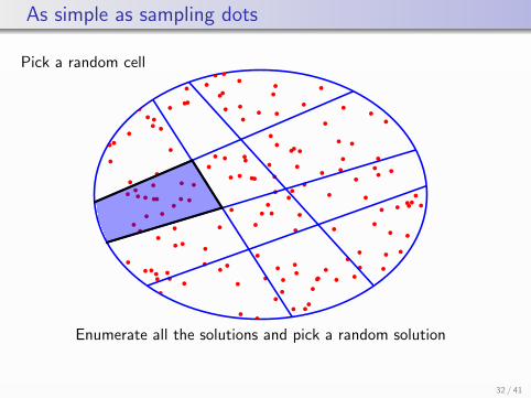
Pick a random cell
Enumerate all the solutions and pick a random solution
32 / 41

As simple as sampling dots
Pick a random cell
Enumerate all the solutions and pick a random solutionChallenge: How many cells?
32 / 41

How many cells?
• Desired Number of cells: 2m∗
= |Sol(ϕ)|thresh
– But determining |Sol(ϕ)| is expensive– ApproxMC(F , ε, δ) returns C such that
Pr[
|Sol(ϕ)|1+ε
≤ C ≤ |Sol(ϕ)|(1 + ε)]
≥ 1− δ
– m = log Cthresh
( m∗ = log |Sol(ϕ)|thresh
)– Check for m = m − 1, m, m + 1 if a randomly chosen cell is small
33 / 41

How many cells?
• Desired Number of cells: 2m∗
= |Sol(ϕ)|thresh
– But determining |Sol(ϕ)| is expensive– ApproxMC(F , ε, δ) returns C such that
Pr[
|Sol(ϕ)|1+ε
≤ C ≤ |Sol(ϕ)|(1 + ε)]
≥ 1− δ
– m = log Cthresh
( m∗ = log |Sol(ϕ)|thresh
)– Check for m = m − 1, m, m + 1 if a randomly chosen cell is small– Not just a practical hack required non-trivial proof
(CMV, CAV13)
(CMV, DAC14)
(CFMSV, TACAS15)
33 / 41

Theoretical Guarantees
Theorem (Almost-Uniformity)
∀y ∈ Sol(ϕ), 1(1+ε)|Sol(ϕ)| ≤ Pr[y is output] ≤ 1+ε
|Sol(ϕ)|
34 / 41

Theoretical Guarantees
Theorem (Almost-Uniformity)
∀y ∈ Sol(ϕ), 1(1+ε)|Sol(ϕ)| ≤ Pr[y is output] ≤ 1+ε
|Sol(ϕ)|
Theorem (Query)
For a formula ϕ over n variables, to generate m samples, UniGen makesone call to approximate counter
34 / 41

Theoretical Guarantees
Theorem (Almost-Uniformity)
∀y ∈ Sol(ϕ), 1(1+ε)|Sol(ϕ)| ≤ Pr[y is output] ≤ 1+ε
|Sol(ϕ)|
Theorem (Query)
For a formula ϕ over n variables, to generate m samples, UniGen makesone call to approximate counter
• JVV (Jerrum, Valiant and Vazirani 1986) makes n ×m calls
34 / 41

Theoretical Guarantees
Theorem (Almost-Uniformity)
∀y ∈ Sol(ϕ), 1(1+ε)|Sol(ϕ)| ≤ Pr[y is output] ≤ 1+ε
|Sol(ϕ)|
Theorem (Query)
For a formula ϕ over n variables, to generate m samples, UniGen makesone call to approximate counter
• JVV (Jerrum, Valiant and Vazirani 1986) makes n ×m calls
Universality
• JVV employs 2-universal hash functions
• UniGen employs 3-universal hash functions
Random XORs are 3-universal
34 / 41

Three Orders of Improvement
Relative Runtime
SAT Solver 1
Desired Uniform Generator 10
UniGen 20
XORSample (2012 state of the art) 50000
Experiments over 200+ benchmarks
35 / 41

Three Orders of Improvement
Relative Runtime
SAT Solver 1
Desired Uniform Generator 10
UniGen 20
XORSample (2012 state of the art) 50000
Experiments over 200+ benchmarksUniGen is highly parallelizable – achieves linear speedup i.e., runtimedecreases linearly with number of processors.
35 / 41

Three Orders of Improvement
Relative Runtime
SAT Solver 1
Desired Uniform Generator 10
UniGen (two cores) 10
XORSample (2012 state of the art) 50000
Experiments over 200+ benchmarksUniGen is highly parallelizable – achieves linear speedup i.e., runtimedecreases linearly with number of processors.Closer to technical transfer
36 / 41

Uniformity
• Benchmark: case110.cnf; #var: 287; #clauses: 1263
• Total Runs: 4× 10⁶; Total Solutions : 16384
37 / 41

Statistically Indistinguishable
• Benchmark: case110.cnf; #var: 287; #clauses: 1263
• Total Runs: 4× 10⁶; Total Solutions : 16384
38 / 41

Beyond Verification
UniGen
HardwareValidation
MusicImprovisation Probabilistic
Reasoning
ProgramAnalysis
ProblemGeneration
39 / 41

Towards Discrete Sampling and Integration
Revolution
40 / 41

Towards Discrete Sampling and Integration
Revolution
• Tighter integration between solvers and algorithms
40 / 41

Towards Discrete Sampling and Integration
Revolution
• Tighter integration between solvers and algorithms
• Exploring solution space structure of CNF+XOR formulas(DMV, IJCAI16)
0 1 2 3 4 5 6
r: Density of 3-clauses
0.0
0.2
0.4
0.6
0.8
1.0
1.2
s:Density
ofXOR-clauses
0.00
0.15
0.30
0.45
0.60
0.75
0.90
1.00
• Can we handle real variables without discretization?
40 / 41

Summary
• Counting and Sampling are fundamental problems in ComputerScience
– Applications from network reliability, probabilistic inference,side-channel attacks to hardware verification
• Hashing-based approaches provide theoretical guarantees anddemonstrate scalability
– From problems with tens of variables to hundreds of thousands ofvariables
Generator RelativeRuntime
SAT Solver 1Desired Uniform Generator 10
UniGen 20UniGen (two cores) 10
XORSample 50000
41 / 41