backtracking dr. jouhaina chaouachi siala. backtracking backtracking is used to solve problems in...
TRANSCRIPT

Backtracking
Dr. Jouhaina Chaouachi Siala

Backtracking
• Backtracking is used to solve problems in which a sequence of objects is selected from a specified set so that the sequence satisfies some criterion.
• Backtracking is used to solve a class of problems known as Constraint Satisfaction Problems (CSP).
• All possible solutions defines the State space of the problem and can be represented as a tree called the State Space Tree.
• Backtracking is a modified depth-first search of a tree.
• Often the goal is to find any feasible solution rather than an optimal solution.
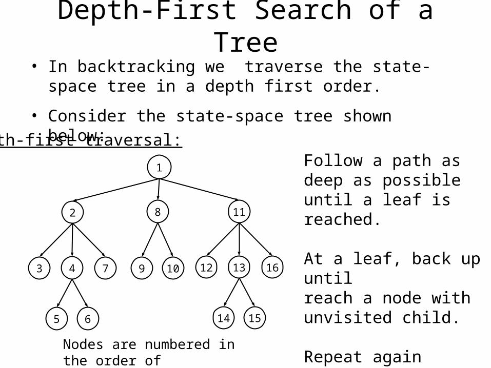
Depth-First Search of a Tree• In backtracking we traverse the state-space tree in a depth first
order.
• Consider the state-space tree shown below:
Nodes are numbered in the order ofa depth-first traversal of the tree.
1
2
3 7
8
4
5 6
11
12 1613
14 15
9 10
Depth-first traversal:Follow a path as deep as possible until a leaf is reached.
At a leaf, back up until reach a node with unvisited child.
Repeat again

Backtracking: n-Queens Problem -I-Problem: Place n queens on an n x n chessboard so that no two
queens threaten each other.
• No two queens threaten each other: Not in the same row.
• Assign each queen to a different row. Each queen can be placed in one of the four columns 4 x 4 x 4 x 4 = 256 possible solutions. 1 2 3 4
1
2
3
4
Q in row 1 is in column 1 1,1 1,2 1,3 1,4
2,1
3,1
4,1 4,4
Checked first. Checked next

Backtracking: n-Queens Problem -II-• Make the search more efficient :
– Not in the same column.– Not in the same diagonal.
1,1 1,2
2,1
x x
2,2
x x x x x x x
3,2
x x x x
4,1 4,4
x x x
2,1 2,2 2,3 2,4
3,1
4,1 4,2 4,3
x x x
x x

• Backtracking: After determining that a node leads to a “dead end” go back to the node’s parent and proceed with search on next child.
• Nonpromising nodes: Cannot lead to a solution• Promising Nodes: May lead to a solution
Backtracking Revisited
1,1 1,2
2,1
x x
2,2
x x x x x x x
3,2
x x x x
4,1 4,4
x x x
2,1 2,2 2,3 2,4
3,1
4,1 4,2 4,3
x x x
x x
Dead endnonpromising
promising

void checknode(node v){ node u; if (promising(v))
if (there is a solution at v)write the solution;
elsefor (each child u of
v) checknode(u);
}
General Algorithm for Backtracking
void df_tree_search(node v){ node u; visit v; for (each child u of v)
df_tree_search(u);}
General recursive Algorithmfor depth first search. General Algorithm for the
Backtracking Approach
• Backtracking algorithm is similar to a depth first search algorithm. Only difference is that in backtracking the children of a node are visited only if the node is promising and no solution at the node.
• Use a function promising called the promising function (different in each application of backtracking) to determine if a node is promising.

void expand(node v){ node u; for (each child u of v) if (promising(u))
if (there is a solution at u)write the solution;
elseexpand(u);
}
Efficient General Algorithm for Backtracking
Efficient General Algorithmfor the Backtracking Approach
• Previously introduced general algorithm for backtracking makes a call to checknode before knowing if the node is promising.
• A more efficient solution could be obtained by visiting only promising nodes.
void checknode(node v){ node u; if (promising(v))
if (there is a solution at v)write the solution;
elsefor (each child u of
v) checknode(u);
}General Algorithm for theBacktracking Approach

bool promising(index i) { index k; bool switch; k =1; switch = true; while (k < i && switch) { if (col[i] = = col[k] || (col[i] - col[k] = =abs(i - k))
switch = false; k++; } return switch;}
The Backtracking Algorithm for the n-Queens Pbcol[i]: column where the queen in the ith row is placed.
void queens (index i) { index j; if (promising(i))
if (i = = n) cout << col[1] through col[n]; else for (j = 1; j <= n; j++) {
col[i + 1] = j; queens(i + 1); }}
if solution found
See if queen in (i + 1)st row can be Positioned in each of the n columns
Check if any queen threatensQueen in the ith row.
If queen in the kth row threatensqueen in the ith row along oneof its diagonals, then:
col(i) - col(k) = i - k or col(i) - col(k) = k - i
If queen in the kth row is in thesame column as queen in the ith row, then:
col(i) = col(k)

Test Run for the n-Queens Problem Algorithm h) backtrack to root <1,2> is promising
i) <2,1> is nonpromising <2,2> is nonpromising <2,3> is nonpromising <2,4> is promising
a) <1,1> is promising
b) <2,1> is nonpromising <2,2> is nonpromising <2,3> is promising
c) <3,1> is nonpromising <3,2> is nonpromising <3,3> is nonpromising <3,4> is nonpromising
d) backtrack to <1,1> <2,4> is promising
e) <3,1> is nonpromising <3,2> is promising
f) <4,1> is nonpromising <4,2> is nonpromising <4,3> is nonpromising <4,4> is nonpromising
g) backtrack to <2,4> <3,3> is nonpromising <3,4> is nonpromising
j) <3,1> is promising
k) <4,1> is nonpromising <4,2> is nonpromising <4,3> is promising
Solution is found.
1,1 1,2
2,1
x x
2,2
x x x x x x x
3,2
x x x x
4,1 4,4
x x x
2,1 2,2 2,3 2,4
3,1
4,1 4,2 4,3
x x x
x x
Root
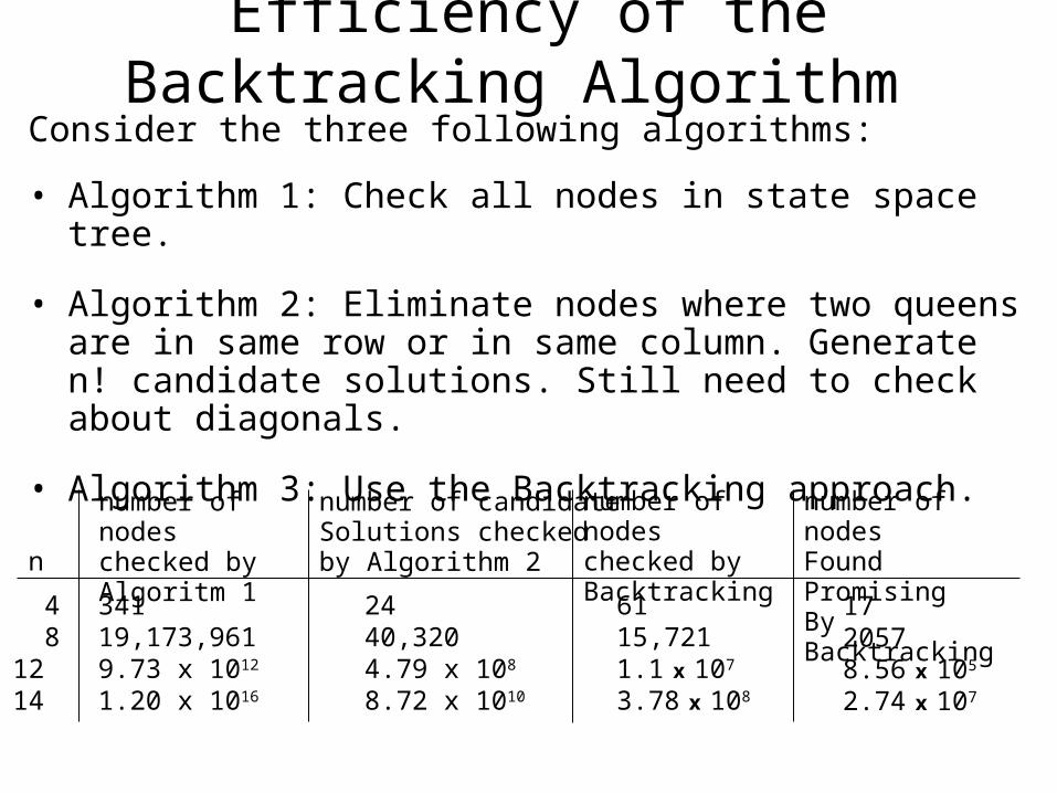
Efficiency of the Backtracking Algorithm Consider the three following algorithms:
• Algorithm 1: Check all nodes in state space tree.
• Algorithm 2: Eliminate nodes where two queens are in same row or in same column. Generate n! candidate solutions. Still need to check about diagonals.
• Algorithm 3: Use the Backtracking approach.
n
4 81214
2440,3204.79 x 108
8.72 x 10¹⁰
6115,7211.1 x 107 3.78 x 10⁸
341 19,173,961 9.73 x 10¹²
1.20 x 10¹⁶
number of nodeschecked by Algoritm 1
number of candidateSolutions checked by Algorithm 2
number of nodeschecked byBacktracking
number of nodesFound PromisingBy Backtracking
1720578.56 x 105 2.74 x 10⁷

Graph Coloring: The m-Coloring Problem• Find all ways to color an undirected graph using at most m colors,
so that no two adjacent vertices are of the same color.
• An important application of the graph coloring problem is map coloring.
• Any map can be represented by a planar graph.
• A graph is called planar if it can be drawn in a plane such that no two edges cross each other.
v1
v3
v2
v4
No solution for the 2-coloring Pb.
v1 color 1v2 color 2v3 color 3v4 color 2
Solution for the 3-coloring Pb:
v1
v3
v2
v4
v5
Map Planar graph
v3
v5
v4
v1
v2

State Space Tree for the m-Coloring Problem• Each path from the root to a leaf is a candidate solution.
• A candidate solution is a solution if any two adjacent vertices are of different colors.
Start
1
1 3
2
2
3
1 32
1 32
Start
1
1 3
2
2
3
1 32
1 32
x x
x x
x
v1
v2
v3
v4
State Space Tree State Space Tree producedby Backtracking

Backtracking Algorithm for the m-Coloring Pbvcol[i]: is the color (integer between 1
and m) assigned to the ith vertexvoid m_coloring (index i) { int color; if (promising(i))
if (i = = n) cout << vcol[1] through vcol[n]; else for (color = 1; color <= m; color++) {
vcol[i + 1] = color; m_coloring(i + 1); }}
bool promising(index i) { index j; bool switch; j =1; switch = true; while (j < i && switch) { if (W[i][j] && vcol[i] = = vcol[j])
switch = false; j++; } return switch;}
if solution found
Try every color for next vertex
Check if an adjacent vertexis already this color
Graph represented by an adjacency matrix . W[i][j] is true if there is an edge between the two vertices i and j otherwise it is false.

Backtracking Approach to the 0-1Knapsack Problem• State space tree is constructed based on whether to include or
exclude item i at level i.
• This is an optimization problem. We can not know if a node contains an optimal solution until the search is over. We will always expand a promising node to look at its children.
• What constitutes a non-promising node so that we can trim the state space tree.
• A node is non promising if:– Total weight at the node is at least the maximum weight– Potential profit for an expansion from that node is not
better than the best profit seen so far. One way to find a bound on this potential is to assume that the entire remaining weight capacity is filled with the most expensive (per weight) items.

Backtracking Approach to the 0-1Knapsack
Problem
• Totweight = weight + wj
• Bound = (profit + pj ) + (W - totweight) x pk/wk
• Bound maxprofit• Bound = 40 + 30 + (16 – 7) x 5 = 115

State Space Tree for 0-1Knapsack Pb. Using Backtracking
Example: 4 items and maximum weight W = 16
Item 1 $40 2
Item 2 $30 5
Item 3 $50 10
Item 4 $10 5
$00
$115
$402
$115
$00
$82
$402
$98
$707
$115
$402
$50
$9012
$98
$9012
$90
$10017$0
$707
$80
$12017$0
(1,1) (1,2)
(0,0)
(2,1) (2,2)
(3,2)(3,1) (3,3) (3,4)
(4,3) (4,4)
P1/w1 = 20
P2/w2 = 6
P3/w3 = 5
P4/w4 = 2 $707
$70
$8012
$80
(4,1) (4,2)
x
x
xxxx
x
Total profits so far
Total weight so far
Bound on total profits
Exclude Item 1
Include Item 1
i pi wi pi/wi
1 $40 2 $202 $30 5 $63 $50 10 $54 $10 5 $2

Test Run of the 0-1Knapsack Backtracking Algorithm 1) maxprft = 0; 2) Visit node (0,0) a) prft = $0; wght = 0; b) bond = $115 3) Visit node (1,1) a) prft = $40; wght = 2; b) maxprft = $40; c) bond = $115
4) Visit node (2,1) a) prft = $70; wght = 7; b) maxprft = $70; c) bond = $115 5) Visit node (3,1) a) prft = $120; wght
=17; b) non prom. c) bond not computed 6) Backtrack to node(2,1)
7) Visit node (3,2) a) prft = $70; wght = 7; b) bond = $80;
8) Visit node (4,1) a) prft = $80; wght = 12; b) maxprft = $80;. c) bond = $80; d) non prom. 9) Backtrack to node(3,2)10) Visit node (4,2) a) prft = $70; wght =7; b) bond = $70 c) non prom.11) Backtrack to node(1,1)
12) Visit node (2,2) a) prft = $40; wght = 2; b) bond = $98
13) Visit node (3,3) a) prft = $90; wght = 12; b) maxprft = $90; c) bond = $98;
14) Visit node (4,3) a) prft = $100; wght = 17; b) non prom.
15) Backtrack to node(3,3)16) Visit node (4,4) a) prft = $90; wght =12; b) bond = $90 c) non prom.17) Backtrack to node(2,2)
18) Visit node (3,4) a) prft = $40; wght = 2; b) bond = $50; c) non prom.
19) Backtrack to root(0,0)
20) Visit node (1,2) a) prft = $0; wght = 0; b) bond = $82; c) non prom.
21) Backtrack to root(0,0)
No more childs !
Done

Branch and Bound (B&B)
• Branch and Bound is very similar to Backtracking.
• Differences with the Backtracking approach are:– Not limited to a depth-first traversal of the state space
tree (any traversal order is OK).– It is used only for optimization problems.
• Visit the best nodes first: Best-first search with B&B pruning.
• Best-first search is a modification of breadth-first search.
• As in the case of backtracking algorithms, B&B Algorithms are usually exponential-time (or worse) in the worst case.

Breadth-First Search of a Tree• In B&B we traverse the state-space tree in a modified version
of a breadth first search.
• Consider the state-space tree shown below:
Nodes are numbered in the order ofa breadth-first traversal of the tree.
1
2
5 7
3
6
13 14
4
10 1211
15 16
8 9
Breadth-first traversal:
Visit the root first.
Visit all nodes at level 1, followed by all nodes at level 2, …
At each level visit nodes from left to right
Level 1
Level 2
Level 3

General Algorithm for Breadth-first Search
void bf_tree_search(tree T){ queue_of_node Q; node u,v;
initialize(Q); v = root of T; visit v; enqueue(Q,v);
while (!empty(Q)) { dequeue(Q,v); for (each child u of v) { visit u; enqueue(Q,v); } }}
• enqueue(Q,v): insert v at the end of the queue Q.
• dequeue(Q,v): Remove v from front of queue Q.
1
2
5 7
3
6
13 14
4
10 1211
15 16
8 9
Q: 1
Q: null; v =1while 1st pass
After for loop: Q: 2,3,4
Q: 3,4; v = 2while 2nd pass
After for loop: Q: 3,4,5,6,7

Breadth-First Search for 0-1 Knapsack Pb. Using B&B
Example: 4 items and maximum weight W = 16
Item 1 $40 2
Item 2 $30 5
Item 3 $50 10
Item 4 $10 5
$00
$115
$402
$115
$00
$82
$402
$98
$707
$115
$402
$50
$9012
$98
$9012
$90
$10017$0
$707
$80
$12017$0
(1,1) (1,2)
(0,0)
(2,1) (2,2)
(3,2)(3,1) (3,3) (3,4)
(4,3) (4,4)
P1/w1 = 20
P2/w2 = 6
P3/w3 = 5
P4/w4 = 2 $707
$70
$8012
$80
(4,1) (4,2)
$00
$60
$305
$82
(2,3) (2,4)
$305
$40
$8015
$82
(3,5) (3,6)
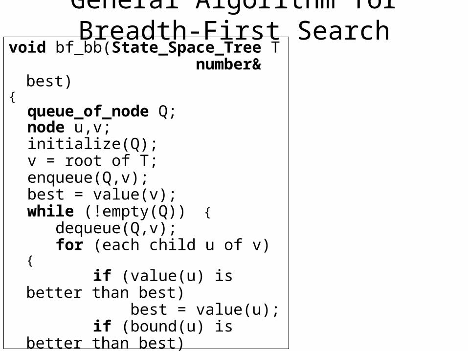
General Algorithm for Breadth-First Searchvoid bf_bb(State_Space_Tree T number& best){ queue_of_node Q; node u,v; initialize(Q); v = root of T; enqueue(Q,v); best = value(v); while (!empty(Q)) { dequeue(Q,v); for (each child u of v) { if (value(u) is better than best) best = value(u); if (bound(u) is better than best) enqueue(Q,u); } }}

void knapsack2(int n, const int p[], const int w[], int W, int& maxprft) { queue_of_node Q; node u,v; initialize(Q); v.level = 0; v.prft = 0; v.wgth = 0; maxprft = 0; enqueue(Q,v); while (!empty(Q)) { dequeue(Q,v); u.level = v.level + 1; u.wght = v.wght + w[u.level]; u.prft = v.prft + p[u.level] if (u.wght <= W && u.prft>maxprft) maxprft = u.prft; if (bound(u) > maxprft) enqueue(Q,u); u.wght = v.wght; u.prft = v.prft; if (bound(u) > maxprft) enqueue(Q,u); }}
float bound(node u) { index j,k int totwght; float result; if (u.wght >= W) return 0; else { result = u.prft; j = u.level + 1; totwght = u.wght; while(j ≤ n && totwght + w[j] ≤ W){ totwght = totwght + w[j]; result = result + p[j]; j+ +; } k = j; if (k <= n) result = result + (W - totwght) x
p[k]/w[k]; return result; }}

General Algorithm for Best-First Searchvoid bestf_bb(State_Space_Tree T number& best){ priority_queue_of_node PQ; node u,v; initialize(PQ); v = root of T; insert(PQ,v); best = value(v); while (!empty(PQ)) { remove(PQ,v); if (bound(v) is better than best) for (each child u of v) { if (value(u) is better than best) best = value(u); if (bound(u) is better than best) insert(PQ,u); } }}

void knapsack3(int n, const int p[], const int w[], int W, int& maxprft) { prty_queue_of_node PQ; node u,v; initialize(PQ); v.level = 0; v.prft = 0; v.wgth = 0; maxprft = 0; v.bond = bond(v); insert(PQ,v); while (!empty(PQ)) { remove(PQ,v); if (v.bound > maxprft) { u.level = v.level + 1; u.wght = v.wght + w[u.level]; u.prft = v.prft + p[u.level] if (u.wght <= W && u.prft > maxprft) maxprft = u.prft; u.bond = bond(u); if (u.bond > maxprft) insert(PQ,u); u.wght = v.wght; u.prft = v.prft; u.bond = bond(u); if (u.bond > maxprft) insert(PQ,u);}} }
float bond(node u) { index j,k int totwght; float result; if (u.wght >= W) return 0; else { result = u.prft; j = u.level + 1; totwght = u.wght; while(j ≤ n && totwght + w[j] ≤ W){ totwght = totwght + w[j]; result = result + p[j]; j+ +; } k = j; if (k <= n) result = result + (W - totwght) x
p[k]/w[k]; return result; }}

Best First State Space Tree for 0-1Knapsack Pb. Using B&B
Example: 4 items and maximum weight W = 16
$00
$115
Item 1 $40 2
Item 2 $30 5
Item 3 $50 10
Item 4 $10 5
$402
$115
$00
$82
$402
$98
$707
$115
$402
$50
$9012
$98
$9012
$90
$10017$0
$707
$80
$12017$0
(1,1) (1,2)
(0,0)
(2,1) (2,2)
(3,2)(3,1) (3,3) (3,4)
(4,1) (4,2)
P1/w1 = 20
P2/w2 = 6
P3/w3 = 5
P4/w4 = 2

Test Run of the 0-1Knapsack Best-First Algorithm 1) Visit node (0,0) a) prft = $0; wght = 0; b) bond = $115 c) maxprft = 0;
2) Visit node (1,1) a) prft = $40; wght = 2; b) maxprft = $40; c) bond = $115
3) Visit node (1,2) a) prft = $0; wght = 0; b) bond = $82 4) Find prom. not
expanded higher bond node: (1,1) a) visit child of (1,1)
5) Visit node (2,1) a) prft = $70; wght = 7; b) maxprft = $70; c) bond = $115
6) Visit node (2,2) a) prft = $40; wght = 2; b) bond = $98
7) Find prom. not expanded higher bond node: (2,1) a) visit child of (2,1)
8) Visit node (3,1) a) prft = $120; wght =17; b) non prom. c) bond = $0
9) Visit node (3,2) a) prft = $70; wght = 7; b) bond = $80; 10) Find prom. not expanded higher bond node: (2,2) a) visit child of (2,2)
11) Visit node (3,3) a) prft = $90; wght = 12; b) maxprft = $90; c) (1,2) , (3,2) become non prom. d) bond = $98;
12) Visit node (3,4) a) prft = $40; wght =2; b) bond = $50 c) non prom.13) Find prom. not expanded higher bond node: (3,3) a) visit child of (3,3)
14) Visit node (4,1) a) prft = $100; wght = 17; b) non prom. c) bond = $0;
15) Visit node (4,2) a) prft = $90; wght = 12; b) bond = $90; c) non prom.
No more promising unexpanded nodes !
Done

Best First State Space Tree for 0-1Knapsack Pb. Using B&B
Example: 4 items and maximum weight W = 16
$00
$120
Item 1 $60 5
Item 2 $30 5
Item 3 $50 10
Item 4 $10 5
$605
$120
$00
$82
$605
$112
$9010
$120
$605
$70
$11015
$112
$11015
$110
$12020$0
$9010
$100
$14020$0
(1,1) (1,2)
(0,0)
(2,1) (2,2)
(3,2)(3,1) (3,3) (3,4)
(4,1) (4,2)
P1/w1 = 20
P2/w2 = 6
P3/w3 = 5
P4/w4 = 2