discount rate heterogeneity among older households: a...
TRANSCRIPT

J Popul Econ (2017) 30:647–680DOI 10.1007/s00148-016-0623-y
ORIGINAL PAPER
Discount rate heterogeneity among older households:a puzzle?
AntoineBozio1,2 ·GuyLaroque2,3 ·CormacO’Dea2
Received: 17 February 2016 / Accepted: 13 October 2016 / Published online: 23 November 2016© The Author(s) 2016. This article is published with open access at Springerlink.com
Abstract We put forward a method for estimating discount rates using wealth andincome data. We build consumption from these data using the budget constraint.Consumption transitions yield discount rates by household groups. Applying thistechnique to a sample of older households, we find a similar distribution to those pre-viously estimated using field data, though with a much lower mean than those foundusing experiments. Surprisingly, among this older population, patience is negativelycorrelated with education and numeracy. This goes against the positive correlationfound for younger populations in experiments and some field studies. We discusspotential explanations for this result.
Keywords Time preference · Discount rate · Consumption
JEL Classifications D12 · D31 · D91 · E21
Responsible editor: Alessandro Cigno
� Cormac O’[email protected]
Antoine [email protected]
1 Paris School of Economics (PSE), Paris, France
2 Institute for Fiscal Studies (IFS), London, UK
3 University College London (UCL), London, UK

648 C. O’Dea et al.
1 Introduction
In many situations, individuals make decisions that involve a comparison of presentand future circumstances. They must decide howmuch to invest in education, howmuchto save for retirement, howmuch to invest in health, etc. In each case, these decisions arebased on some assessment of the potential welfare at different periods under differentscenarios. FollowingSamuelson (1937), economists have largely adopted a discounted-utility model which assumes that preferences over time can be condensed into onemajor parameter, the geometric discount rate (see Frederick et al. 2002 for a criticalreview and Hall 2010 for a review of recent research developed using this approach).
To estimate discount rates, both field data and experiments are found in the lit-erature. Experimental studies are by far the most numerous. Among the 42 studiessurveyed by Frederick et al. (2002), 34 use experimental methods. A typical approachis for individuals to be offered a menu of (real or hypothetical) choices between aquantity of money now and a different quantity of money at some point in the future.Respondents’ choices are used to estimate a discount rate.
Our paper fits into a much smaller literature that estimates discount rates usingfield data on aspects of behaviour and a lifecycle model of consumption and saving. Atypical way to estimate preference parameters in such models, though not the one thatwe will take, has been to solve numerically the intertemporal optimisation problemthat the agents in a particular population are assumed to face. Estimates of parame-ters such as the discount rate are chosen such that the model’s predictions are close,in some metric and according to some data, to those seen in reality. Such studies varyin the extent to which heterogeneity in the discount factor is admitted into the model.Some papers assume homogenous discounting behaviour, like French (2005) andEdwards (2013) where discounting is exponential and Laibson et al. (2007) wherediscounting is quasi-hyperbolic. More flexibility was allowed by Attanasio et al.(1999) who estimate a version of the lifecycle model where the discount rate variesstochastically with the composition of the household while even more is allowedby Samwick (1998) and Gustman and Steinmeier (2005) who estimate a differentdiscount rate for every household.
These papers fully specify a lifecycle model and solve it. The method we employdoes not do this but rather uses the first-order condition to that solution—the Eulerequation. We first generate longitudinal observations on consumption using a pro-cedure introduced by Ziliak (1998) and Browning and Leth-Petersen (2003). Thisinvolves calculating consumption using comprehensive and high quality data onassets and income and the intertemporal budget constraint. Our resulting distribu-tion of consumption is shown to be remarkably similar to that derived from theUK’s household budget survey. Using the Euler equation and consumption tran-sitions at the household level, we estimate average discount rates for groups ofhouseholds. Such an approach has typically been precluded in the past by theabsence of good quality panel data on consumption—a problem discussed in detail byBrowning et al. (2003).
Our approach has some parallels with papers that have previously relied on theEuler equation to estimate parameters, in particular the elasticity of intertemporalsubstitution. Estimation in this manner was carried out by Campbell and Mankiw

Discount rate heterogeneity 649
(1989) and Attanasio and Weber (1995) among others. For a lively criticism of thisapproach, see Carroll (2001) and for a defense see Attanasio and Low (2004). Ourapproach differs from these papers in three principal ways. First, we are able to useconsumption transitions at the household level rather than relying on aggregate orcohort-level data. Second, our use of household rather than cohort level consumptiondata allows us to use the exact Euler equation in our estimation, rather than relyingon Taylor series approximations. Third, we do not assume that the discount rate isthe same for each individual in our sample, nor do we assume that it is unchangingacross the lifecycle.
We apply the procedure outlined above to a representative sample of older Englishhouseholds using the English Longitudinal Survey of Ageing (ELSA). We show,unsurprisingly, that there is substantial heterogeneity in discounting in that popula-tion. The typical levels of discount rates that we estimate are of similar magnitudeto those estimated in other papers based on the lifecycle model of consumption andsaving. These rates imply substantially less discounting than is implied by the resultsof experimental studies.
Our most surprising result is that discount rates tend to rise with education andlevels of numerical ability (i.e. those with less education and those who are lessnumerically able tend to be the most patient). This result is contrary to that found inthe literature that measures the extent to which individuals discount future incomestreams (see for instance Warner and Pleeter 2001; Harrison et al. 2002; Dohmenet al. 2010). These papers differ in their empirical approach—the first uses data onthe choices of departing military personnel over whether they will take their sever-ance payment in a lump-sum or in the form of an annuity payment, while the secondand third papers use laboratory experiments. The literature using field data offersless conclusive evidence. Gourinchas and Parker (2002) solve a lifecycle model andestimate discount rates by matching simulated consumption data to those observedin the data at different ages and, similar to us, finds that people with more educa-tion are less patient. On the contrary, Cagetti (2003), implementing a broadly similarprocedure as that used by Gourinchas and Parker, but using data on assets instead ofconsumption, finds evidence suggesting the more educated are more patient. This isalso found by Lawrance (1991), using an approach based on a log-linearised Eulerequation and data on transitions in food expenditure.
We discuss our somewhat puzzling result below and raise the possibility thatprior evidence, driven largely by choices individuals made at younger ages is notapplicable to the discounting between periods at older ages.
The rest of this paper is structured as follows. Our empirical approach is outlinedin Section 2. In Section 3, we describe the data and explain how we calculate con-sumption from assets and income. Results are presented in Section 4 and discussedin Section 5. Section 6 concludes.
2 Theory and empirical approach
In our estimation of discount rates, we start from a standard life-cycle model inwhich each household (as a collective unit) maximises expected discounted utility by

650 C. O’Dea et al.
choosing their consumption and their holdings of each of J different asset or debtinstruments each period. In period t , household i faces the following optimisationproblem:
max{Xj
is ,cis }Ts=t
u(cit ) +T∑
τ=t+1
(τ−t∏
s=1
1
1 + ρi(t+s)
)E [u(ciτ )]
subject to the constraints
(i)
pτ ciτ +∑
jp
j
(τ+1)Xj
i(τ+1) = eiτ +diτ +∑
jrjτ pj
τ Xjiτ +
∑jpj
τ Xjiτ ∀ τ (1)
(ii)X
j
i(τ+1) ≥ bj
i(τ+1) ∀ τ, j (2)
where ρit is the discount rate for household i between period t and t + 1. Equation 1is the budget constraint at date τ and Eq. 2 represents a borrowing constraint for assetj : bj is the minimum level of that asset that must be held. This will be negative fordebt instruments that households have access to and zero for non-debt instruments.1
The other quantities in the model are consumption (ct ), holdings of each of J assets(Xj
t ) which are negative in the case of debts, the nominal income yield of asset j (rjt ),
the price of asset j (pjt ), labour income (et ), income from transfers (dt ) and the price
of consumption (pt ). We make the standard assumption that the instantaneous utilityfunction u(.) is invariant over time.
An Euler equation (first-order condition) is satisfied for every asset that house-holds can potentially hold (see for example Campbell 2000). That is, for each assetj , and for each pair of consecutive periods t and t +1, the following inequality holds:
du(cit )
dcit
≥ 1
(1 + ρi(t+1))E
[(1 + r
j
t+1
) pt
p(t+1)
du(ci(t+1))
dci(t+1)
](3)
The Euler equation holds at equality for household i as long as the sales of assetj are not constrained (i.e. as long as X
j
it+1 > bj
it+1). In particular, the consumptionof households who hold positive cash balances satisfies (where 0 indexes cash):
du(cit )
dcit
= 1
(1 + ρi(t+1))E
[(1 + r0t+1
) pt
p(t+1)
du(ci(t+1))
dci(t+1)
](4)
All features of the model other than the instantaneous utility function are allowedto vary freely over time—in particular, we do not assume that the discount rate istime-invariant.
We specify the utility function as taking the familiar isoelastic form:
u(c) = c1−γ
1 − γ(5)
1Alternatively, we could specify a liquidity constraint that ensures that total debts are no greater than acertain quantity.

Discount rate heterogeneity 651
where γ is the coefficient of relative risk aversion. Assuming that constraints on cashholdings do not bind, the discount rate is given by (suppressing i subscripts):
ρt+1 = E
[(1 + r0t+1
) pt
pt+1
(ct
ct+1
)γ ]− 1. (6)
This equation forms the basis for our empirical approach. We group householdsaccording to particular characteristics (such as their education level, numerical abil-ity, age and marital status) and estimate the expectation in the equation above byusing the sample average of the quantity in square brackets among households of aparticular group. In using the sample average to estimate the expectation term, weneed to assume that there are no differential shocks across households that lead tosystematic differences in the term pt
pt+1
(ct
ct+1
)γ
.
It is worth pointing out how the change in consumption (the central observablequantity that enters the Euler equation) identifies the discount rate. The faster is con-sumption growth, all else being equal, the lower is the discount rate (that is, themore patient is the individual concerned). Households who are patient tend to forsakecurrent consumption for future consumption—and therefore exhibit consumptiongrowth. The converse is also true. Those who are impatient tend to prefer currentconsumption to future consumption. They therefore have lower (or even negative)consumption growth.
To bring Eq. 6 to the data, we need to specify an interest rate on cash and a coeffi-cient of relative risk aversion. We now discuss each of these in turn. Figure 1 showsthe nominal pre-tax rate of return on two types of cash assets in the UK between2002 and 2009—instant access savings and time deposits. Until the large fall in thelast quarter of 2008, interest rates were relatively stable, moving within a range ofapproximately a percentage point. In our estimation, we use a nominal pre-tax inter-est rate of 3 %—approximately the average rate of return on time deposits over theperiod. Our headline results refer to the consumption changes over the period 2004
01
23
4
Inte
rest rate
2002m1 2004m1 2006m1 2008m1 2010m1
Month
Time deposits Instant access
Fig. 1 Nominal pre-tax rate of return on cash in the UK – 2002 to 2009

652 C. O’Dea et al.
to 2006 and will therefore be unaffected by the large fall in interest rates in 2008.With some exceptions, interest is taxable in the UK and we convert this pre-taxinterest rate to a post-tax interest rate using the marginal rate of tax faced by eachhousehold in a particular year. For couples whose members face different marginaltax rates, we use the lower of the two rates, on the basis that efficient tax-planningin most cases will allow the couple to pay that lower rate of tax on their assetincome.
We cannot identify the coefficient of relative risk aversion (γ in Eq. 6) and weassume that is does not vary across individuals. The assumption of a coefficient ofrelative risk aversion that does not vary across households is a strong one (Outreville2015 surveys the empirical literature which has shown differences in risk aversionexist by education group). However, our data does not contain sufficient individualvariation in interest rates to warrant identification. We set γ equal to 1.25. This isconsistent with the range of elasticities of intertemporal substitution estimated byAttanasio and Weber (1993) on UK data and very close to that obtained by Gustmanand Steinmeier (2005). We have generated results assuming alternative values of γ .While the mean discount rates are sensitive to these values, the ranking of house-holds’ discount rates is the same for all positive choices of γ that are constant acrosshouseholds.
Finally, it is worth making explicit two restrictions implicit in the use of Eq. 6.These relate to liquidity constraints and changes in the utility function due tochanging household composition or changing labour supply.
First, recall that the Euler Eq. 6 only holds at equality when individuals are not liq-uidity constrained. If we use Eq. 6 to estimate the discount rate for a group containingliquidity constrained individuals, the estimate will be biased downwards. Concernsabout the presence of liquidity constraints in our case are mitigated by the fact thatwe work on a population over the age of 50, at a point in the lifecycle where mosthave accumulated some liquid wealth—almost 95 % of our sample have positivegross liquid asset holdings. As a check that our results are not being driven by liquid-ity constraints, we have confirmed that there are no substantial changes in focusingonly on those with liquid assets above a certain minimum level (see Section 5).
Second, when individuals leave or join a household between periods, the assump-tion of a constant instantaneous utility function at dates t and t + 1 does not makesense; we therefore do not include households whose composition changes betweenwaves of data. Further, as evidence points to changes in consumption patterns aroundretirement (Banks et al. 1998; Wakabayashi 2008), we exclude from our samplehouseholds where some member left the labour market during the period covered byour data.
The previous two paragraphs have outlined two exclusions from our estimatingsample. Some further exclusions are necessary due to the fact that we are not able tocalculate consumption satisfactorily for every household in our sample. The extentof these exclusions is outlined in the Appendix. To deal with the fact that thoseomitted are unlikely to be a random sub-sample of our overall sample, we generateweights representing the probability of each household being included in our sam-ple and, in our results we attach a weight to each household of the inverse of this

Discount rate heterogeneity 653
probability. These probabilities are estimated as functions of marital status, edu-cation, age, income quintile and wealth quintile. Our results will, therefore, berepresentative of the entire population aged 50 and over if the selection into oursample can be adequately modelled as a function of these characteristics.
3 Data
Our data come from the English Longitudinal Study of Ageing (ELSA). ELSA isa panel survey that is representative of the English population aged 50 and over. Itstarted in 2002, and individuals have been re-interviewed every 2 years since then—our main results use data from the first three waves. The purpose and form of thesurvey is similar to the Health and Retirement Study (HRS) in the US and the Surveyof Health, Ageing and Retirement in Europe (SHARE) in 20 European countries.The first wave was conducted between April 2002 and March 2003 and sampled12,099 individuals (of whom 11,391 were core sample members; the remainder wasindividuals aged under 50 who were the partners of core sample members). There are7894 benefit units (i.e. a single person or couple along with any dependent children)where each member of the couple is a sample member. Our sample is drawn fromthese benefit units.
While ELSA contains questions on some components of expenditure (food,domestic fuel and clothing) it does not, unfortunately, contain data on total expendi-ture, which, approximating consumption, is needed to estimate the discount rate. Infact, there is no nationally representative longitudinal survey that collects total expen-diture in the UK and such data is rare internationally.2 This lack of comprehensivelongitudinal data on expenditure has proved something of an obstacle to bringingEuler equations to data. The literature has either relied on aggregate data, or, follow-ing Browning et al. (1985), has used repeated cross-sections to form a quasi-panelof birth cohort-level average expenditure. An alternative approach was suggested bySkinner (1987) and refined by Blundell et al. (2008). It involves estimating the rela-tionship between food (and possibly other items of) expenditure and total expenditureusing a household budget survey. As general-purpose panel surveys often containdata on food expenditure, this estimated relationship can be used to impute totalexpenditure.
We proceed in a different manner: following Ziliak (1998) and Browning andLeth-Petersen (2003), we use the rich data on income and assets that is contained inELSA to back out expenditure from the intertemporal budget constraint. In all thefollowing, we will equate total expenditure (excluding mortgage repayments) withconsumption. The rest of this section summarises this procedure—further details aregiven in the Appendix—and shows a close correspondence between features of the
2A notable exception to this is the Spanish ‘Encuesta continua de presupuesto familiares’, a diary-basedlongitudinal survey of expenditure. The Panel Study of Income and Dynamics in the US, since 1999, hascollected expenditure data that covers approximately 70 % of average total expenditure.

654 C. O’Dea et al.
resulting distribution of consumption with those that are obtained using the UK’sHousehold Budget Survey.
3.1 Calculating consumption using longitudinal data on assets and income
We use longitudinal data on assets and income along with the budget constraint tocalculate consumption between two waves. Equation 1 can be re-arranged to get thevalue of consumption in period t as follows:
ptct = et + dt +∑
j
rjt p
jt X
jt +
∑
j
(p
jt X
jt − p
j
t+1Xj
t+1
)(7)
The timing convention and how it relates to the data deserves some discussion. InELSA, interviews take place approximately every two years. So to be precise,
• Flow variables representing consumption ct , non-capital income et , transfers dt
and the asset yield, including any capital gain or loss, rjt , are measured over the
entire two year period;• Stock variablesX
jt represent holdings of assets at the beginning of the period (i.e.
at the time of the first interview); Xj
t+1 represents asset holdings at the beginningof period t + 1 or equivalently at the end of period t (i.e. at the time of the nextinterview);
• Asset prices pjt and p
j
t+1 represent asset prices at the time of the first and secondinterview;
• The overall price level pt represents the average price level in the period betweenthe two interviews.
Equation 7 is the equation that we use to calculate consumption between twowaves of the survey. Having calculated consumption in this manner, we make onefurther adjustment and subtract mortgage repayments (both capital components andinterest) from the resulting quantity. While these represent cash expenditure onhousing, they are not generally indicative of consumption of the flow of housingservices.
Equation 7 can be rewritten as:
ptct = et + dt +∑
j
(q
jt + p
j
t+1 − pjt
pjt
)p
jt X
jt +
∑
j
(p
jt X
jt − p
j
t+1Xj
t+1
)(8)
where the rate of return on asset j , rjt has been written as the sum of the income yield
qjt and the capital gain
pj
t+1−pjt
pjt
earned during period t .
Some, but not all of the quantities on the right-hand-side of Eq. 8 can be directlyread from the ELSA data. In each wave the value of each asset held (pjXj ) isrecorded, as are non-capital income (e), capital income (qjpjXj ) and lump-sumtransfers (d) in the period prior to the interview (where ‘period’ in the case of most

Discount rate heterogeneity 655
forms of income and transfers represents 12 months). ELSA respondents are askedfor details on 16 different financial asset and (non-mortgage) debt instruments.3
These include various type of savings products, bond holdings and equity holdings.See Section A.1.1 in the Appendix for more detail and Table 10 in that section forsummary statistics on holdings in each asset.
Our data does not record capital gains on assets held between the two waves
(p
j
t+1−pjt
pjt
), nor does it contain data on income and transfers for a period of approx-
imately one year (recall that ELSA sample members are surveyed approximatelyevery two years) - two objects that appear in Eq. 8. The majority of assets held bythe population in our sample are in safe forms—so there is no capital gain to be con-sidered for these assets. For equity holdings, we assume a capital gain (or loss) inline with the change in the FTSE index between the two interview dates. Estimatingincome in the missing year is facilitated by exploiting the longitudinal aspect of thesurvey data—we interpolate linearly between income in year y and income in yeary + 2 to obtain income in year y + 1. Finally, we assume that there are no lump-sum transfers in the missing year and we exclude from our sample those householdswhere it is likely that some member received a lump-sum transfer (due to retirement,redundancy or the death of a spouse or parent). We give further details about all ofthese assumptions and their implications in the Appendix.
3.2 Comparing consumption in ELSA and in the EFS
In this section, we compare the distribution of consumption estimated in the man-ner described above with that estimated using the Expenditure and Food Survey(EFS).4 The EFS is the UK’s household budget survey, and is used to calculate thecommodity-weights of the UK’s inflation indices (the Consumer Prices Index and theRetail Prices Index). The data is collected annually, throughout the year and the sur-vey is designed to be nationally-representative. Respondents are asked to record allpurchases over a 2-week period in a diary and also to complete a questionnaire thatseeks information on infrequently-purchased items. The combination of the diary andthe questionnaire allows a comprehensive measure of consumption to be calculated.
Figure 2 shows the cumulative distribution function and the probability densityfunction of total consumption in both surveys. The data shown is for calendar year2003 for the EFS and for (annualised) calculated consumption between the surveysin 2002/03 and 2004/05 for ELSA. The EFS functions are estimated using only thosehouseholds where the head is aged over 50 so that both samples are drawn frompopulations with the same age profile. Both distributions are shown net of mortgagerepayments. As mentioned at the end of Section 1 and discussed in the Appendix, tocompute the distribution of consumption in ELSA, we weight each observation by
3There are also questions on housing wealth, physical wealth and pension wealth.4This survey has, since 2008, been known as the Living Costs and Food Survey. However, the data that weshow is from years prior to this, so we make use of the older name.

656 C. O’Dea et al.
0.2
.4.6
.81
CD
F
0 10000 20000 30000
Consumption
0.0
00
02
.00
00
4.0
00
06
.00
00
8
De
nsity
0 10000 20000 30000
Consumption
EFS ELSA EFS ELSA
Fig. 2 CDF and PDF of consumption in EFS and ELSA—2003
the inverse of the probability of being able to calculate consumption. In both surveys,we trim the most extreme values—showing the middle 80 % of the distribution.
Figure 2 shows that there is a close correspondence between the distributions inboth shape and location. The correspondence is closest at the bottom of the distri-bution (i.e. up to annual consumption of £10,000). At this point, the distributionsdiverge somewhat—with the distribution of consumption in ELSA lying to the rightof that in the EFS. This divergence, which represents a tendency for consumption tobe greater in ELSA than the EFS in the upper half of the distribution, is consistentwith the fact that consumption in the EFS (grossed up to national levels) is knownto under-record the level of consumption calculated as part of the National Accountswith the degree of under-reporting thought to be greater for those who have higherlevels of consumption (see Brewer and O’Dea 2012).
3.3 Summary statistics
We noted at end of the last section (and give more detail in Appendix A.4.1) thatsome households are omitted from the sample (for example, because the data ontheir asset holdings had to be imputed and therefore we are not confident in thequality of our consumption data). Table 1 gives summary statistics, both for the full

Discount rate heterogeneity 657
ELSA sample and our sample. Panel (A) gives proportions in categories of age, edu-cation, numerical ability and marital status: these are the variables which we useto group households in estimating discount rates (6).5 Panel (B) gives means andselected percentiles of the distribution of annual income, net liquid wealth and nethousing wealth. Comparisons between the two sets of statistics shows that there is aclose correspondence between the characteristics of our sample and the full ELSAsample—with the exception that our sample under-represents those with the highestliquid wealth holdings.
4 Results
We first summarise the distribution of the quantities represented by the right-handside of Eq. 6:
[(1 + r0t+1)
pt
pt+1
(ct
ct+1
)γ ]− 1 (9)
This quantity would be equal to the discount rate if ct+1 and pt+1 were perfectlyforecasted by households at date t . Our presentation of the distribution of this quantitywhich we refer to below as the ‘ex-post’ discount rate is a useful preliminary step.
Our use of four waves of ELSA data gives us up to three observations on consump-tion for each household and therefore up to two observations on the ex-post discountrate. Figure 3 shows two distributions of the ex-post discount rates (trimming the bot-tom 10 % and top 10 % of the sample). The median discount rate is approximately−3 % in the earlier period and is 0 % in the later period. These median ex-post dis-count rates are low relative to estimates of the discount rate found in the literaturethat estimate such rates using field data and very low relative to those found in theexperimental literature.
Figure 3 shows substantial heterogeneity around these medians. This depicts thedistribution of the discount rate, perturbed by two phenomena. First, realisations ofstochastic variables will differ from their expectations. Second, our consumption datais likely to include some measurement error. Figure 3 also shows the distributionof the geometric mean of our two successive observations on the discount rate. Thevariance of this distribution is substantially smaller than the variance of either cross-sectional distribution. This could be due to some combination of averaging over time
5Those who did not complete UK school leaving exams (typically taken at the age of 18) have ‘low’education, those who completed these but have no third-level education are in the ‘middle’ educationgroup, and those with any post-schoolqualification are in the ‘high’ education group. Numerical ability istested using six questions in ELSA—our categorisation follows that in Banks et al. (2010). Marital statusis defined covering the first four waves of ELSA - those whose status changed are in the ‘other’ group.The age, education and numerical ability of the couple are taken as that of the older/more educated/morenumerically-able of the couples. More details on the education and numerical ability characteristics aregiven in Appendix A.1.2.

658 C. O’Dea et al.
Table 1 Summary statistics
(A) (B)
All Our All Our
Households sample Households sample
Age groups (props.) Annual income (£1000s)
50–59 34.45 34.13 Mean 17.01 17.14
60–69 26.78 25.29 p10 5.08 5.14
70–79 23.84 23.95 p25 7.58 7.70
80+ 14.93 16.63 p50 12.69 13.30
Total 100.00 100.00 p75 21.10 21.58
p90 32.36 31.09
Education (props.) Net liquid wealth (£1000s)
Low 54.70 54.65 Mean 73.28 45.00
Middle 28.57 28.24 p10 0.00 0.00
High 16.66 17.10 p25 1.61 2.00
Total 100.00 100.00 p50 13.50 11.52
p75 61.55 51.60
p90 169.00 121.36
Numerical Ability (props.) Net housing wealth (£1000s)
1(Lowest) 11.89 9.73 Mean 114.11 117.03
2 41.22 40.97 p10 0.00 0.00
3 29.95 32.53 p25 0.00 20.00
4(Highest) 15.47 16.07 p50 90.00 95.00
Missing 1.47 0.70 p75 161.00 175.00
Total 100.00 100.00 p90 250.00 260.00
Marital status (props.) Sample size
Single 7.19 8.42 7,894 1,504
Marr/cohab 52.08 54.32
Widowed 24.12 26.23
Sep/Div 10.48 11.03
Other 6.15 0.00
of the discount rate for each family and to a diminished effect of measurement erroronce we take a time average.
We are aware of three papers that, using field data and the lifecycle model,have estimated the entire distribution of discount rates: Alan and Browning (2010),Samwick (1998) and Gustman and Steinmeier (2005) (hereafter GS). In Table 2, wecompare our three distributions of the ex-post discount rate (the two cross-sectionaldistributions, and the distribution of their geometric average) to those found in the

Discount rate heterogeneity 659
0.0
1.0
2.0
3.0
4
Density
40 20 0 20 40 60
Ex post discount rate
2004/06 2006/08 Average
Fig. 3 Distribution of ex-post discount rates – 2004/06, 2006/08 and average
last two of these using a breakdown reported in GS.6 It is important to note, though,that we would not necessarily expect a close correspondence between our results andtheirs as the populations on which the estimates are based are very different. Ourresults are for English households containing an individual aged over 50, while theresults of both Samwick and GS are estimated on samples of US working-age adults.
The most striking difference between our results and those of Samwick and GS isthe substantial number of households that we find with ex-post discount rates of lessthan 5 %. We find approximately 60 % here in this portion of the distribution com-pared to approximately 40 % in the distribution of discount rates in the two papersbased on the US all-age population. We find a larger share of households with neg-ative ex-post discount rates (approximately 50 % of the sample). This compares toapproximately 10 % of those in Samwick’s sample (see his Fig. 3; note that GS donot report the proportion with negative discount rates).
In our two cross-sectional distributions, we find a similar share of households inthe right tail of the distribution (those with a discount rate greater than 15 %) as doSamwick and GS, and find less mass in the region of 5 to 15 %. On our averagemeasure, the mass in the left tail of our distribution increases, largely at the expense,relative to either cross-sectional distribution, of that in the right tail.
The models of both Samwick and GS assume a discount rate for a particularhousehold that does not change over time. If discount rates do vary over time, their
6These results are not directly comparable with those in Alan and Browning (2010) where the distributionsare presented graphically. Additionally, that paper discusses how their results relate to those in Samwick(1998). Alan and Browning (2010) restrict the discount rate to be greater than 0. We find, as do GS andSamwick, evidence of households with negative discount rates.

660 C. O’Dea et al.
Table 2 Comparison of our results with those of Samwick (1998) and Gustman and Steinmeier (2005)
Discount Samwick GS Ours Ours Ours
rate 04–06 06–08 Ave
<5 % 38 % 40 % 60 % 56 % 67 %
5–10 % 25 % 21 % 5 % 6 % 9 %
10–15 % 10 % 6 % 5 % 6 % 7 %
>15 % 25 % 33 % 30 % 32 % 17 %
NOTES: These groups are those reported in Gustman and Steinmeier’s Table 2. That table does not showthe proportion with negative estimated discount rates. Our three estimated distributions have proportionswith negative estimated discount rates of 53, 48 and 56 %, respectively
estimates represent some average of the lifetime sequence of discount rates. There-fore, the large mass that we find in the left tail of the distribution could be reconciledwith the estimates of Samwick and GS if households have higher discount rates atyounger ages than at older ages (at which point they enter our population of interest).
Table 3 gives estimates of the median ex-post discount rate (ρ̂) and associated stan-dard errors of the medians (σ ), for groups defined according to age, marital status,education, numerical ability (we discuss how these last two variables are constructedin Appendix). No clear relationship with age is evident7 while the evidence is sug-gestive that, if anything, those who are widowed or divorced are more patient inthis period than those who are single and never married and those who are married.Surprisingly, we find that less educated families and families with lower levels ofnumerical ability tend to be more patient than those with more education and greaterlevels of numerical ability respectively (though the differences are less pronouncedin the latter case).
We use a grouping estimator to estimate the average ex-ante discount rate forgroups defined by age, marital status, levels of education and numerical ability. Theestimator is based on Eq. 6. It estimates the expectation in that equation by its sampleanalogue for a particular group and weights the results to account for possibly non-random selection into our sample. For each group, we trim the sample, removingthose in the first and tenth decile of consumption growth. Unlike Alan and Browning(2010), we do not explicitly account for the role of measurement error. However, ourapproach does not involve assuming (as does the vast majority of work in this area)that preference parameters remain the same over the whole of the lifecycle.
Table 4 summarises these results. The results mirror those presented above inTable 3—no clear relationship with age; widows and those who are divorced appear-ing more patient than those who are otherwise single and those who are married; andevidence that discount rates increase with education and numerical ability.
7While we refer to (the absence of) a relationship with age, we are not able to separately identify asso-ciations of discount rates with each of age and cohort. Exploiting a longer panel than we have access towould allow us to separately identify age and cohort effects if we assumed that there were no time effectsin discount rates.

Discount rate heterogeneity 661
Table 3 Median ex-post discount rate by household characteristics
Age ρ̂ σ Marital status ρ̂ σ Education ρ̂ σ Numerical ability ρ̂ σ
50–59 −2.2 2.4 Single 0.1 5.3 Low −3.2 1.0 1 (Low) −2.9 2.0
60–69 −4.6 1.9 Married −2.1 2.1 Mid. −1.8 2.1 2 −3.2 1.1
70–79 −2.5 1.4 Widowed −3.1 1.7 High 6.5 5.6 3 −0.8 2.7
80+ 0.5 2.5 Sep./Div. −4.8 2.1 4 (High) −1.3 4.0
All −2.3 1.0 All −2.3 1.0 All −2.3 1.0 All −2.3 1.0
NOTES: The number of households in each of the age groups are 350, 432, 492 and 229. The numberof households in each of the marital status groups are 133, 619, 510 and 241. The number of householdsin each of the education groups are 942, 396 and 165. The number of households in each of the fournumeracy groups are 189, 699, 431 and 174. The median in the ‘All’ row differs slightly between columnsas the number of households in each differs. In calculating the ‘All’ group median, we exclude those withmissing values of the covariate in question
The magnitude of the differences between the education groups is large.8 Forexample, the difference between the point estimates of the mean discount rate for the‘low’ education group and those in the ‘high’ education group is over 9 percentagepoints. This means that, over this period and in this population, if those with the mosteducation are to exhibit the same saving behaviour at the margin as those with theleast, the former group will require a safe return of 9 percentage points greater thanthe latter group.
Table 5 investigates the joint association between average discount rates, educa-tion and numerical ability. Here, those in numeracy groups 1 and 2 are categorisedas having ‘low’ numerical ability and those in numeracy groups 3 and 4 are cate-gorised as having ‘high’ numerical ability. The ‘low’ education group is defined asbefore, while the ‘med./high’ education group contains the upper two categories. Thegradient of the association between education and average discount rate, conditionalon level of numerical ability is particularly large. Among those with low levels ofnumerical ability, the average discount rates of the low education group is estimatedat −3.1 %, compared to 1.0 % for those in the mid./high education group. For thosewith more numerical ability, the differences according to education are starker—withaverage discount rates of −1.5 % and 4.6 % for those with less and more education,respectively.
Table 6 explores the robustness of our most puzzling result—the fact that esti-mated mean discount rates are higher for those with more education than those withless. Column 1 is associated with less trimming than in our headline results. We trimthose in the bottom and top 5 % of the distribution of consumption growth instead ofthose in the bottom and top 10 %. Columns 2 and 3 apply successively stricter sam-ple selection rules than are applied in our baseline sample. These are the ‘middle’and ‘strict’ sample selection rules outlined in Appendix A.4. In the first two cases,
8The differences are also statistically significant. The difference between the mean discount rates of thelow and middle education groups are significant at the 5 % level and those between the high and loweducation group are significant at the 1 % level.

662 C. O’Dea et al.
Table 4 Mean ex-ante discount rate by household characteristics
Age ρ̂ σ Marital status ρ̂ σ Education ρ̄ σ Numerical ability ρ̄ σ
50–59 −0.0 1.4 Single 1.2 2.2 Low −2.6 0.7 1 (Low) −2.9 1.4
60–69 −1.8 1.2 Married 2.0 1.2 Mid. 0.8 1.4 2 −2.4 0.8
70–79 −0.7 1.1 Widowed −3.2 1.0 High 6.7 3.0 3 1.6 1.5
80+ −0.5 1.7 Sep/Div −3.8 1.2 4 (High) 2.3 2.4
All −0.9 0.6 All −0.9 0.6 All −0.9 0.6 All −1.0 0.6
NOTES: The sample sizes in each category are smaller here than in Tables 3 as, in each category we trimthe top and bottom 10 % of values. The number of households in each of the age groups are 280, 343, 392and 183. The number of households in each of the marital status groups are 107, 499, 408 and 193. Thenumber of households in each of the education groups are 749, 319 and 133. The number of householdsin each of the four numeracy groups are 153, 561, 345 and 140. The mean in the ‘All’ row differs slightlybetween columns as the number of households in each differs. In calculating the ‘All’ group median, weexclude those with missing values of the covariate in question
the results that we previously emphasised still hold—the estimated mean discountrates are higher for those with more education than those with less. In columns 2 and3, as the sample becomes more restricted and smaller, the gradients are less clearlymonotonic and the standard errors are larger.
We might want to confirm that our relatively small sample, combined with ourtrimming of the largest 10 % increases in consumption and largest 10 % decreases inconsumption does not materially affect our results. To investigate this, we solve andsimulate behaviour from a simple life-cycle model. We specify a life-cycle modelwhere agents make a consumption and saving choice every year from the age of20 to 100. In each period until the age of 65 they receive income which follows anautoregressive process with autocorrelation of 0.95 and variance of 0.02. We specifythat there are equal numbers of ten types of agents, each with a different discountrate. Discount rates range from −2.5 to 7.5 % with a mean of 2.5 %.
After solving (using a backwards recursion) for the set of consumption functions,we carry out the following procedure 499 times. First, we draw a sample of 200agents (20 from each discount rate type). Second, we simulate their consumptionbehaviour using the calculated consumption functions. Third, we take one consump-tion transition between two sequential years for each individual. The age for thetransition is chosen as a random age between 50 and 80; this age differs for eachindividual. We then trim the largest and smallest 10 % of consumption transitionsand estimate a discount rate (just as we do in our estimation). The mean (across 499
Table 5 Mean ex-ante discountrate for groups defined bypairwise combinations of botheducation and numerical ability
Low education Med./High education
Low numeracy −3.1 1.0
(0.8) (1.8)
High numeracy −1.5 4.6
(1.5) (1.9)Standard errors are inparentheses

Discount rate heterogeneity 663
Table 6 Sensitivity of meanex-ante discount rate for groupsdefined according to education
(1) (2) (3)
Education ρ̄ σ ρ̄ σ ρ̄ σ
Low −1.0 0.9 −1.5 0.9 −0.6 1.3
Mid. 3.9 1.8 2.7 1.8 3.0 2.6
High 10.5 3.6 3.9 4.2 −0.3 6.8
All 2.1 0.8 −0.5 0.8 −0.3 1.2The total sample size is 1355 incolumn (1), 776 in column (2)and 305 in column (3)
simulations) estimated discount rate is 2.37 % with a 95 % confidence interval of[2.16 %, 2.59 %] which contains the truth. This simulation reassures us that estima-tion of the discount rate in sample sizes of the type that we have is possible withreasonable precision.
5 A puzzling result?
Our results are puzzling in light of the studies, particularly those using experimen-tal designs, that find that low educated individuals tend to lack patience compared tohigher educated. A primary difference between this paper and most of the rest of theliterature is the fact that results in the latter come from samples of individuals whotend to be much younger than ours. Work using lifecycle models (e.g. Samwick 1998;Gustman and Steinmeier 2005) typically focuses on working age individuals whilethe experimental literature often uses samples of students. In contrast, our samplecomprises older households in England, aged 50 and above. Frederick et al. (2002)noted at that time that ‘no studies [had] been conducted to permit any conclusionsabout the temporal stability of time preferences’ and, while Bishai (2004) does inves-tigate how time preference changes over the age range 14 to 37, we are not aware ofany studies that look at the discounting behaviour of the oldest households. We nowbriefly consider some other explanation for our results.
First, consider survival probabilities. Households in the model discount the futurefor two reasons—first their ‘pure’ rate of time preference, and second their expec-tation of being alive at each period in the future. Differential survival probabilitiescould explain our result on education in the following manner. Suppose that all edu-cation groups had the same mean ‘pure’ discount rate, but that one group had a longerlife-expectancy. This group would appear to be more patient. A negative correlationbetween education and life expectancy could explain, at least some of, our results.In our data, however, it is those with lower education levels that tend to have shorterlife expectancies. ELSA respondents are asked the following question: ‘What are thechances that you will live to be X or more?’, where X depends on their current age.We run a simple linear regression of the responses to this question on dummies forour education groups and age dummies (the latter to account for the possibility thatthose in different education groups are distributed differently across ages). We findthat those in the middle education consider themselves to be 3.1 percentage points

664 C. O’Dea et al.
more likely to live to the age referenced in the question than those in the low edu-cation group, and those in the high education group are 5.4 percentage points morelikely. Differential life expectancies, therefore, would seem to work in the oppositedirection from our puzzle.
Second, if it were the case that those with more education had access to higherpre-tax safe rates of return, then our assumption that everyone has the same pre-taxrate of return would generate a downward bias in the estimates of discount rates forthe more educated relative to the less. That those with more education might face(through greater financial literacy) higher rates of return is plausible. This wouldrender our result a conservative one—and the actual gap between the discount rate ofthose with less and more education could be greater than that which we find.
Third, liquidity constraints might be important. Recall that for any household thatis liquidity constrained, the Euler equation (which forms the basis for our estimatingEq. 6), will hold with an inequality rather than an equality. Our sample is comprisedof those over the age of 50 who are substantially less likely to be liquidity constrainedthan those earlier in their lifecycle; Table 10 in the Appendix shows that 93 % ofour sample have positive holdings of gross liquid assets. To investigate a potentialdifferential incidence of liquidity constraints between those with different levels ofeducation and numerical ability, we show results for samples restricted to those withholdings of at least £2500, £5000 and £10,000 of gross liquid assets, respectively.Table 7 shows the results for these sub-samples for our groups defined by educa-tion. The gradient of interest—that patience is decreasing in education—is apparentin each of the sub-samples. While the populations represented by each of thesesub-samples differ in important ways (because, for example, wealth is endogenousto the discount rate), we interpret these results as strongly suggestive that liquid-ity constraints are not driving our headline associations between discount rates andeducation.
A fourth consideration is the possible incidence of non-insured shocks that dif-fer systematically between the groups we examine. The effect of these will not beremoved from the grouping estimator that we implement. The ELSA data allows usto indirectly assess whether these may be important. There is a question which asks‘What are the chances that at some point in the future you will not have enoughfinancial resources to meet your needs?’. Figure 4 shows the distribution of changesin financial insecurity reported by individuals between waves 1 and 3 for the three
Table 7 Mean ex-ante discountrate for groups definedaccording to education and levelof positive gross liquid assets
Level of positive liquid gross assets
Base ≥ 2,500 ≥ 5,000 ≥ 10,000
Education ρ̄ σ ρ̄ σ ρ̄ σ ρ̄ σ
Low −2.6 0.7 −5.2 1.0 −5.3 1.3 −5.2 1.8
Mid. 0.8 1.4 −0.2 1.8 −0.4 2.1 −1.9 2.4
High 6.7 3.0 8.0 3.4 8.7 3.4 6.9 3.6
All −0.9 0.6 −2.4 0.9 −1.0 1.1 −1.2 1.4
The total sample size is 1,200 inthe base category, 818 in thesample of those with over£2,500, 641 in the sample withover £5,000 and 497 in thesample with over £10,000

Discount rate heterogeneity 665
0.0
1.0
2.0
3
Density
100 50 0 50 100
Change
Low Mid High
Fig. 4 Variation in financial insecurity by education level
different education groups. There is a peak at no change for all three educationgroups - with no evident differences in the location between groups. Linear regres-sions of these changes on education dummies and dummies for numerical abilityreveal no (even marginal) statistically significant differences between groups. Wetake this as suggestive evidence that there were not substantial differential shocksacross education groups over our data period.
As a fifth check, it is useful to assess, to the extent that we can with our short panel,whether the relationship between education and the discount rate is also found usingconsumption transitions between time periods other than those we have focussed onabove. The results described in the previous section are generated using differencesin consumption between the period 2002–2004 (between waves 1 and 2 of ELSA)and the period 2004–2006 (between waves 2 and 3 of ELSA). We have also esti-mated discount rates using the change in consumption between this second period and
Table 8 Mean ex-ante discountrate between two different set ofyears
2002/04–2004/06 2004/06–2006/08
Education ρ̄ σ ρ̄ σ
Low −2.6 0.7 0.7 0.7
Mid. 0.8 1.4 −0.2 1.3
High 6.7 3.0 12.4 2.5
All −0.9 0.6 2.0 0.6

666 C. O’Dea et al.
Table 9 Discount rates andhousing price growth (1) (2) (3)
Mid Education 1.33 −0.04 −0.06
High Education 9.62*** 9.87** 9.87**
Housing wealth effect −0.02
Constant −3.16*** −3.41* −3.42*
Observations 1,503 986 986***p<0.01, **p<0.05, *p<0.1
2006–2008 (the period between waves 3 and 4 of ELSA). These results are shown inTable 8, alongside our baseline results. The differences in patience between the mostand least educated group are larger in the case of the latter pair of years, though thereis little difference over that period between the estimated discount rates between thelower two education groups.
A sixth check that we make is whether increases in housing wealth (that wereperhaps unanticipated) over the period we consider could explain the greater growthin consumption among the more educated. We investigate this by running a medianregression of the ‘ex-post’ discount rate on education dummies and a variable thatgives the increase in housing wealth between the first and third waves of ELSA (2002and 2006) as a proportion of initial wealth. The results are given in Table 9. Column(1) shows the results of a median regression on education dummies for our full sam-ple. Column (2) shows the results of this regression applied to the 65 % of our samplewho own their own property. Column (3) adds to this the increase in housing wealthas a proportion of total wealth. This coefficient is insignificant and the other coeffi-cients barely change. We interpret this as evidence that changes in house prices andtheir effect on consumption do not explain our results.
As a final comment, we acknowledge the role that measurement error could playin our results. Note that classical measurement error, for example with a constantvariance error that is multiplicative with consumption, will affect the level of theestimated discount rates but not affect the relative position of the groups. One needsa non-standard type of measurement error (for instance multiplicative with highervariance among those with more education relative to those with less) to undo ourresults.
6 Conclusion
This paper puts forward a method for estimating individual discount rates usingfield data. We build consumption panel data from the intertemporal budget constraintand panel data on income and wealth. This household-level panel data is used, withthe Euler equation, to estimate discount rates for groups defined by socio-economiccharacteristics.
We show, unsurprisingly, that there is substantial heterogeneity in discounting inour sample which is drawn from a population of older households. But surprisingly,

Discount rate heterogeneity 667
we find that, among this older population, households with less education and lowernumerical ability exhibit greater patience than, respectively, those with more educa-tion and greater numerical ability. This result, which is robust to differential housingwealth shocks, differential mortality and differential incidence of liquidity con-straints is somewhat puzzling as it is the opposite to that found in investigations oftime preference for younger households.
Acknowledgments Co-funding is acknowledged from the European Research Council (referenceERC-2010-AdG-269440—WSCWTBDS) and the Economic and Social Research Council (Centre forMicroeconomic Analysis of Public Policy reference RES-544-28-5001). Thanks to James Banks, RichardBlundell, James Browne, Rowena Crawford, Mariacristina De Nardi, two anonymous referees and to sem-inar participants at the Institute for Fiscal Studies, the Paris School of Economics and the Economic andSocial Research Institute of Ireland for valuable comments. Any errors are our own.
Compliance with ethical standards
Funding This study was funded by the European Research Council (reference ERC-2010-AdG-269440– WSCWTBDS) and the Economic and Social Research Council (Centre for Microeconomic Analysis ofPublic Policy reference RES-544-28-5001).
Conflict of interest The authors declare that they have no conflict of interest.
Open Access This article is distributed under the terms of the Creative Commons Attribution 4.0International License (http://creativecommons.org/licenses/by/4.0/), which permits unrestricted use, dis-tribution, and reproduction in any medium, provided you give appropriate credit to the original author(s)and the source, provide a link to the Creative Commons license, and indicate if changes were made.
Appendix
This appendix gives additional detail on the data that we use, our mr calculating con-sumption and the derivation of the sampling weights that we use. Section A presentsstatistics on the measures of wealth, education and numeracy in ELSA. Section Bdetails the procedure by which we computed consumption from our panel data onwealth and income. Section C presents additional comparisons of our estimates ofconsumption from ELSA data with the consumption data available in EFS. Section Dpresents the characteristics of the final sample and, addressing concerns about our useof a non-random sub-sample of the population, discusses the construction of surveyweights.
A.1 Data
The data we utilise in this paper is the English Longitudinal Study of Ageing (ELSA).ELSA is a biennial longitudinal survey of a representative sample of the Englishhousehold population aged 50 and over (plus their partners). The first wave wasconducted between April 2002 and March 2003 and sampled 12,099 individuals (ofwhom 11,391 were core sample members; the remainder were individuals aged under50 who were the partners of core sample members). There are 7894 benefit units (i.e.

668 C. O’Dea et al.
a single person or couple along with any dependent children) containing a samplemember. Our sample is drawn from these benefit units.
ELSA collects a wide range of information on individuals’ circumstances. Thisincludes detailed measures of their financial situation: income from all sources(including earnings, self-employment income, benefits and pensions), non-pensionwealth (including the type and amount of financial assets, property, business assetsand antiques) and private pension wealth (including information on past contri-butions and details of current scheme rules). ELSA also collects information onindividuals’ physical and mental health, cognitive ability, social participation andexpectations of future events (such as surviving to some older age or receiving aninheritance).
A.1.1 Data on household wealth
Given the importance of the wealth measure for our estimation, it is worth detailinghow it is measured in the survey. ELSA respondents are asked for details on 16 dif-ferent financial asset and (non-mortgage) debt instruments.9 For each asset (X), the‘main respondent’ in each benefit unit is asked: ‘Howmuch do you/you and your hus-band/wife/partner currently have in X?’. If the respondent does not know or refusesto say, a series of questions is asked that attempts to put lower and upper bounds onthese assets. An imputation procedure is then carried out that gives a point estimatefor the asset level for these individuals.10
Table 10 summaries the holdings in each of these assets. Some are self-explanatory(e.g. cash savings), others are specific to the UK and deserve some comment.Cash ISAs (Individual Savings Account) and TESSAs (Tax-Exempt Special SavingsAccount) are tax efficient cash savings which are subject to annual limits on what canbe paid in. Stocks and shares ISAs and Personal Equity Plans (PEPs) are stocks andshares held in a tax-efficient ISA (Individual Savings Account) and are also subjectto annual limits on what can be paid in. Life insurance savings ISA are life insurancesavings held in a tax-efficient vehicle. Bonds could be either savings bonds (withretail banks) or government/corporate bonds. According to the ONS (2009) (Table4.1) fewer than 2 % of households directly hold government or corporate bonds whileover 8 % hold fixed-term bonds with financial institutions. Therefore, households inELSA who report holdings of ‘bonds’ are more likely to be holding savings bonds(which are effectively fixed-term risk free savings accounts) than gilts or corporatebonds. National savings are cash savings held in the a government-owned agency(‘National Savings and Investment’). Finally, premium bonds are also issued by the
9There are also questions on housing wealth, physical wealth and pension wealth.10This imputation procedure, carried out by the ELSA team is called a conditional hot-deck. Given that weknow the, say, cash holdings of a particular household are between £a and £b—that individual is assigneda random draw from the empirical asset distribution of those who report their assets exactly as between £aand £b and have the same characteristics along some dimensions: here it is age and household composition.

Discount rate heterogeneity 669
Table 10 Holdings of different financial assets
(1) (2) (3) (4) (5) (6)
Asset Mean Mean Med Proportion Mean Prop.
(Uncond.) (Cond.) (Cond.) with asset port. share unimp.
Cash Savings 12,111 13,474 4000 90.1 % 54.9 % 80.4 %
Cash ISAs 2436 7452 6000 34.1 % 10.0 % 91.6 %
TESSAs 1457 9796 9000 16.7 % 3.5 % 95.3 %
National savings 832 11,547 3000 9.2 % 1.8 % 96.6 %
Premium bonds 763 2373 100 33.6 % 2.6 % 95.7 %
Bonds 2837 29,425 16,000 11.6 % 3.6 % 95.2 %
Shares 6650 22,087 3500 31.6 % 7.5 % 88.8 %
S&S ISAs 1551 11,982 7000 14.8 % 2.9 % 92.3 %
PEPs 2792 18,158 9000 17.2 % 3.7 % 93.1 %
Invest. trusts 2379 26,483 12,000 10.9 % 2.5 % 94.8 %
Life ins. savings 2267 22,470 10,000 12.0 % 4.5 % 93.2 %
Life ins. ISAs 91 9974 2000 3.0 % 0.2 % 95.4 %
Other savings 2179 40,458 15,000 7.4 % 2.4 % 96.9 %
Total 38,346 41,258 12,152 93.1 % 100.0 % 64.7 %
NOTES: Column (1): mean holdings in the asset, unconditional on having a positive holding (in GBP);column (2): mean holdings in the asset, conditional on having a positive holding; column (3): medianholdings in the asset, conditional on having a positive holding; column (4): the proportion benefit unitsthat holds this asset; column (5): the mean portfolio share (among those with positive total gross assets);column (6): the proportion of benefit units who report their exact holdings and so for whom no imputationis necessary
SOURCES: ELSA, wave 1 (2002/03)
government. Instead of yielding interest, the holders of these bonds are included in amonthly draw for large cash prizes.
The ELSA survey asks also for details on three different types of non-mortgagedebt. These are credit card debt, private debt (i.e. debts to friends and family) and‘other debt’ (primarily overdrafts and personal loans). Table 11 summarises theholdings of different debt instruments and has a form similar to Table 10.
A.1.2 Data on education and numerical ability
We outline here how our measures of education and numerical ability are defined.We categorise individuals into one of three education groups on the basis of the
highest qualification that they have. We consider those who have a third-level degreeor higher to have a ‘high’ level of education. Those who have A-levels (Britishschool-leaving exams, taken at age 18) or equivalent but no university degree arein the ‘mid’ education group. All others are in the ‘low’ group. Our measure of

670 C. O’Dea et al.
Table 11 Balances of different debts
(1) (2) (3) (4) (5) (6)
Debt type Mean Mean Med Proportion Mean Prop.
(Uncond.) (Cond.) (Cond.) with ass. port. share uinimp.
Credit card debt 369 1,989 800 20.3 % 41.1 % 98.8 %
Private debt 68 5,612 1,000 3.3 % 2.8 % 99.3 %
Other debt 846 3,904 1,500 23.3 % 56.1 % 98.9 %
Total 1,293 4,067 1,400 31.8 % 100.0 % 97.1 %
NOTES: See notes to Table 10
SOURCES: ELSA, wave 1 (2002/03)
consumption, and therefore our estimates of discount rates, are at the household (for-mally benefit unit11) level. We need an education measure, therefore, at the householdlevel. We take the education of a household containing a couple to be the greater ofthe two levels of education held by the adults in that couple.
Numerical ability is measured in ELSA using a series of six questions, which arereproduced in Box 1. The simplest of these questions requires the respondent to solvea very simple exercise in subtraction while the most difficult requires the respondentto solve a problem involving compound interest. We divide all individuals into oneof four groups following the categorisation in Banks et al. (2010). Mirroring ourapproach with respect to education, we take the numerical ability of a householdcontaining a couple to be the greater of the two levels of numerical ability held bythe two members of that couple.
Box 1 Numerical Ability in ELSA
1. If you buy a drink for 85 pence and pay with a one pound coin, how muchchange should you get?
2. In a sale, a shop is selling all items at half price. Before the sale a sofa costs£300. How much will it cost in the sale?
3. If the chance of getting a disease is 10 per cent, how many people out of 1,000would be expect to get the disease?
4. A second hand car dealer is selling a car for £6,000. This is two-thirds of whatit cost new. How much did the car cost new?
5. If 5 people all have the winning numbers in the lottery and the prize is £2million, how much will each of them get?
6. Let’s say you have £200 in a savings account. The account earns ten per centinterest per year. How much will you have in the account at the end of twoyears?
11A benefit unit is a single adult or couple along with any dependent children that they have. Relativelyfew members of our sample have dependent children, so our results can be thought of as representingsingle adults and couples.

Discount rate heterogeneity 671
A.2 Computing consumption
In this subsection, we present some additional details on the consumption calculationprocedure. We reproduce Eq. 8 here, which makes clear the data requirements:
ptct = et + tt +∑
j
(q
jt + p
j
t+1 − pjt
pjt
)p
jt X
jt +
∑
j
(p
jt X
jt − p
j
t+1Xj
t+1
)(10)
Three issues that we now discuss in turn are the following:
1. How to estimate capital gains on assets held between the two waves
(p
j
t+1−pjt
pjt
)
2. How to estimate income and transfers for the first half of the period betweenwaves. This is necessary as ELSA sample members are surveyed approximatelyevery two years with the questionnaire seeking, in most cases, data on receiptsin the past year, rather than on over the entire period between waves
3. Whether to make adjustments to the procedure when asset stocks in either waveare imputed
A.2.1 Estimating capital gains
We need to estimate capital gains on assets held between two waves
(p
j
t+1−pjt
pjt
).
Depending on the type of asset we make different assumptions.
i. For cash or most cash-like assets (savings, TESSAs, National savings, Prize
bonds) and ‘other savings’, we assume no capital gain
(p
j
t+1−pjt
pjt
= 0
).
ii. For Cash ISAs and Bonds,12 we have a concern that some respondents, forwhom their interest income is simply being rolled up in their account and notwithdrawn, will report that their ‘income’ is zero, when in fact it is positivebut simply saved. If income from the asset is reported as positive, we assumethat there is no change in the value of the asset. If, however, individuals reportzero income from their holdings (and approximately 39 % of bondholders doin wave 1), we assume that they are, in fact, receiving interest and that thisinterest is simply accumulating in their account and they don’t as a result con-sider it as ‘income’. We assume that they earn a rate of return equal to themedian rate of return for those holding similar assets who do report incomeand reflect this interest in an increase in the ‘value’ of the asset. That is, forindividuals who hold the particular asset but who report no income, we assume
that, if the median return on that asset in that wave was 2 % thenp
jt+1−p
jt
pjt
=(1.02)τ − 1, where τ ≈ 2 is the length of time in years between the twointerviews.
12These are largely bank savings bonds (i.e. effectively fixed term savings accounts) rather thangovernment or corporate bonds.

672 C. O’Dea et al.
iii. For equities and equity-like assets, we make a distinction whether the incomefrom the asset is reported as positive or zero. If income is reported as posi-tive, we assume that the value of the asset increased in line with the FTSE 100price index (which excludes dividend payments) between the dates of the twointerviews. If income is reported as zero, we assume that the value of the assetincreased in line with the FTSE 100 total return index (i.e including dividendpayments) between the dates of the two interviews.
iv. For debt, we assume that the interest rate on credit card debt is 15 %, the interestrate on ‘other debt’ (mostly overdrafts) is 8 % and that there is a 0 % interestrate on ‘private debt’.
A.2.2 Imputing missing income
For each month between the waves where we do not have income data, we interpolatelinearly between the two income observations that we have. We carry out this proce-dure separately for each category of income (employment income, self-employmentincome, private pension income, state pension income, benefit income, asset incomeand other income).
We vary the procedure in two cases. The first of these is when respondents donot report some category of their income exactly in one (but not both) of the waves(i.e. they perhaps only give bounds). In these cases we assume that income has beenequal over the period to the value in the year for which we have full information. Thesecond case where we vary the procedure is when it comes to state pension income.Here we use the data on the age of the respondents and the state pension age toestablish when their state pension payments started.
A.2.3 Whether to make adjustments to the procedure when asset stocks in eitherwave are imputed
In a number of cases, survey respondents do not know the exact amount of some assetholding or some income component. In that case, the ELSA questionnaire attemptsto obtain bounds on the unknown amounts and the survey data is published withimputed amounts that lie between these bounds.
When individuals report that they do not know exactly their holdings in any par-ticular wave t or t + 1 (i.e. they don’t know X
jt or X
j
t+1 for some j ), we make theassumption that they made no payments into or withdrawals from their assets—i.e.X
jt − X
j
t+1 = 0.
A.3 Comparisons of consumption measures between EFS and ELSA
Figures 5, 6 and 7 probe the comparison between the distribution of consumption inthe EFS and in ELSA more deeply than in the body of the paper. The figures eachtake a particular household characteristic (age, education and marital status respec-tively) and compare the conditional distributions of consumption in both surveys. Weshow the 25th, 50th and 75th percentiles as well as the mean. Of interest are both

Discount rate heterogeneity 673
05,0
00
10,0
00
15,0
00
20,0
00
25,0
00
Consum
ption
p25 p50 p75 Mean
50 55 60 65 70 75 50 55 60 65 70 75 50 55 60 65 70 75 50 55 60 65 70 75
EFS ELSA
Fig. 5 Comparing consumption in EFS and ELSA—by age—2003
the difference between quantiles for a households of a particular type (for example,whether the shape and location of the distributions match for young people) and thedifferences for a particular quantile across household types (for example, whether therelationship between median expenditure and age is similar in both surveys).
These figures show that many of the points we made above in our comparison ofthe unconditional distributions of consumption between surveys are true for the dis-tributions conditional on (at least these) household characteristics. For all age groups,for those with middle and higher levels of education and for all marital statuses, the75th percentile of consumption is higher in ELSA than in the EFS, and in most casesthe median and mean are higher too, with smaller differences to be seen between the25th percentiles in each survey. The socio-economic gradients observed in the EFSare closely replicated in the ELSA consumption data – that is consumption decreaseswith age, rises with education and married households consume more than singlehouseholds (unsurprisingly as our measure of consumption here is not adjusted usingan equivalence scale).
As a final comparison of our generated data on consumption with that in the EFSwe make use of the fact that data on food spending is recorded in ELSA. In Fig. 8, weplot the relationship between food spending and total spending in both surveys (againtrimming the bottom and top 10 % of consumption). The relationships shown areestimated using locally-weighted regressions. Food spending is estimated as greaterin ELSA than in the EFS;13 the slope of the relationship between it and total spending
13One potential reason for this is the different methods by which the data on food spending is gathered.The ELSA data is taken from respondents’ responses to a question that asks how much they spend on foodin a typical month. The EFS data is taken from respondents’ spending diary entries.

674 C. O’Dea et al.
05
,00
01
0,0
00
15
,00
02
0,0
00
25
,00
0
Co
nsu
mp
tio
n
p25 p50 p75 Mean
Low Mid High Low Mid High Low Mid High Low Mid High
EFS ELSA
Fig. 6 Comparing consumption in EFS and ELSA – by education – 2003
is, however, similar in both surveys from the point at which total consumption is equalto approximately £10,000. Below this level, food spending in ELSA does not varymuch with our calculated measure of total consumption—an indication, perhaps, thatsome of the households in the left-tail of the distribution of consumption are theredue to measurement error.
A.4 Selection and composition of sub-sample
To balance considerations of maintaining as large a sample as is possible and of usingas little inaccurate data as is possible, we exclude observations where we feel the datadid not allow us to estimate consumption. We provide here details on how our samplewas selected (D.1) and then we describe the selected sample and the construction ofweights used to correct for our use of a non-representative sample in (D.2).
A.4.1 Selection of the sample
We exclude benefit units from the our estimating sub-sample if any of the followingconditions hold.
1. If at least one component of income is not known up to a closed interval in bothwaves t and t + 1.
2. If a ‘large’ change in physical wealth was observed between the two waves.Changes in the financial asset values that we observe could then be the result of

Discount rate heterogeneity 675
05,0
00
10,0
00
15,0
00
20,0
00
Consum
ption
p25 p50 p75 Mean
M. S. W. D. M. S. W. D. M. S. W. D. M. S. W. D.
EFS ELSA
Fig. 7 Comparing consumption in EFS and ELSA—by marital status—2003
transferring asset holdings between types of assets rather than being indicativeof consumption. We define a large change in ‘physical assets’ as occurringwhen there has both been a change in the value of holdings of at least £2,000and a proportionate change in the value of the portfolio of at least 30 %
3. If a ‘large’ change in uncategorised wealth was observed between the twowaves. A small number of couples keep their finances largely separate. When
1500
2000
2500
3000
3500
4000
Food s
pendin
g
0 10000 20000 30000 40000
Consumption
EFS ELSA
Fig. 8 Comparison of relationship between food spending and consumption in EFS and ELSA—2003

676 C. O’Dea et al.
these individuals are asked for any asset holdings that they hold jointly, onlythe total level of jointly-held asset is sought - not the level of holdings of par-ticular assets. Estimating the capital gain between waves is thus not possible. Alarge change is the value of joint holdings is considered to have occurred whenthere has both been a change in the value of holdings of at least £2,000 and aproportionate change in the portfolio of at least 30 %
4. If an individual bought or sold a house between the waves5. If mortgage payments are missing6. If some critical piece of data is missing (usually education or age), the impu-
tation procedure used by the ELSA team to fill in missing income and assetholdings is not possible
7. If the benefit unit composition changed between the two waves8. If the either partner in a couple does not respond to the survey9. If a lump-sum payment has been received in the past year and we do not observe
the exact amount10. If either member of a benefit unit suffered the bereavement of their last remain-
ing living parent between waves (and thus may have received an inheritance thatwe might not observe if was received over a year before the ELSA interview)
Table 12 summarises the selection operated by our procedure from the initialsample. We need two successive observations on assets to compute consumption –therefore the left panel shows the proportions for whom we have a successful con-sumption calculation as a proportion of the 6,022 benefit units who make up thebalanced panel for waves 1 and 2 (the panel on the right of the table shows these pro-portions out of all those observed in wave 1. The rules we have established above leadus to exclude 38 % of the balanced panel. For an additional 2.3 % of the sample, weestimate negative consumption level, indicative of a failure to impute consumption.
Table 13 summarises the proportions of benefit units in the balanced panel wherea particular reason for the consumption calculation being unsuccessful is relevant.
We described above how we deal with cases where some component of assets orincome is not known exactly and have had to be imputed. Where assets are not knownin either wave, we assume that there has been no flow in or out between waves. Wethus do not use the imputed data on assets. We do, on the other hand, use the imputeddata on income, but exclude benefit units where at least one component of income
Table 12 Success rate ofconsumption calculation Proportions of Proportions of
balanced panel wave 1 sample
Computation status Obs. Percentage Obs. Percentage
Have consumption 3,541 58.8 % 3,541 44.8 %
Calculation failed 2,298 38.2 % 2,298 29.1 %
Negative consumption 183 3.0 % 183 2.3 %
Attrited – – 1,872 23.7 %
Total 6,022 100.0 7,894 100.0 %

Discount rate heterogeneity 677
Table 13 Summary of reasonsfor consumption calculationfailing
Reasons Percentage
Missing income component 760 12.6
Large change in physical wealth 721 12.0
Large change in uncategorised wealth 85 1.4
Bought or sold property 321 5.3
Mortgage payments missing 48 0.8
Critical information missing 181 3.0
Benefit Unit composition changed 145 2.4
Non-responding partner 416 6.9
Missing data on lump-sum receipt 141 2.3
Last surviving parent died 352 5.9
is not known up to a closed interval in both waves t and t + 1. We have assessed if(and confirmed that) our results hold if we apply stricter sample selection rules withrespect to the use of imputed data. The third and fourth panels in Table 6 for example,show the estimated discount rates with successively stricter sample selection rulesthan applied in the baseline (in the text of the paper we have referred to these as our‘middle’ and ‘strict’ sample selection rules). These rules are as follows:
• Middle: Do not include individuals when the value of some asset holding in wavet is not known at least up to a closed interval. Do not include individuals where atleast one component of income is not reported exactly in both waves t and t + 1.
• Strict: Do not include individuals when the value of some asset holding in wave t
is not reported exactly. Do not include individuals where at least one componentof income in wave t is not reported exactly in either wave t or t + 1.
The foregoing tables and discussion detail the extent to which we have been ableto calculate consumption. To estimate a discount rate we need, of course, at least twosuccessive observations on consumption (and therefore three successive observationsin the data). There are 4,886 benefit units in the balanced panel of the first threewaves of data. Of these we can include 1,578 (32 %) of these in our estimating sub-sample. We exclude benefit units where the consumption calculation failed betweeneither pair of waves (1 and 2 or 2 and 3), where calculated consumption is less than£3,000 in either case or where the benefit unit composition or labour supply activity
Table 14 Summary of reasons for consumption calculation failing
Reasons Percentage
Consumption calculation failed between either pair of waves 2,532 51.8
Consumption less than £3000 between either pair of waves 780 16.0
Benefit unit composition changed 1,103 22.6
Labour supply changed 690 14.1

678 C. O’Dea et al.
of either member changed. Table 14 shows the number (and proportion) of cases inwhich these conditions are relevant.
A.4.2 Characteristics of the selected sample
With a successful calculation of consumption for approximately 60 % of the balanced(wave 1 and 2) panel, and the inclusion in the estimating sub-sample of approximately
Table 15 Logit regression of successfully calculating consumption on sample on characteristics
Probability of being in Probability of being in
consumption sample discount rate sample
(1) (2) (3) (4)
Age 50 to 54 (omm.)
Age 55 to 59 0.98 1.12 0.94 0.99
Age 60 to 64 1.00 1.11 0.99 1.07
Age 65 to 69 1.15 1.31*** 1.77*** 2.07***
Age 70 to 74 1.30*** 1.69*** 1.95*** 2.56***
Age 75 to 79 1.21* 1.88*** 1.66*** 2.56***
Age 80 to 84 0.95 1.70*** 1.35** 2.48***
Age 85 or over 0.59*** 1.82*** 0.76 2.44***
Single (omm.)
Married 0.81** 0.77** 0.77** 0.83
Widowed 1.30*** 1.12 1.10 0.88
Separated 1.29** 1.24 1.33** 1.29
Low Educ. (omm.)
Mid. Educ. 1.15** 0.98 1.14 0.94
High. Educ. 1.03 0.89 0.96 0.80*
Inc. quint. 1 (omm.)
Inc. quint. 2 1.01 0.94 0.94 1.00
Inc. quint. 3 1.09 0.97 0.90 0.83*
Inc. quint. 4 1.05 1.00 0.87 0.86
Inc. quint. 5 1.01 0.92 0.66*** 0.61***
Wealth quint. 1 (omm.)
Wealth quint. 2 0.83** 0.45*** 0.71*** 0.49***
Wealth quint. 3 0.72*** 0.33*** 0.57*** 0.33***
Wealth quint. 4 0.56*** 0.22*** 0.41*** 0.22***
Wealth quint. 5 0.35*** 0.13*** 0.21*** 0.11***
Observations 7,253 5,476 7,253 4,439
NOTES: In specifications (1) and (2) the sample is all those sampled in wave 1, regardless of whetherthey attrited by wave 2 or not. In specification (3) the sample is the balanced (wave 1 and 2) panel. Inspecification (4), the sample is the balanced (waves 1, 2 and 3) panel
***p<0.01, **p<0.05, *p<0.1

Discount rate heterogeneity 679
32 % of the balanced (waves 1 to 3) panel, there might be some concern about therepresentativeness of the sample. In this section we describe the dimensions alongwhich these samples are non-random.
Table 15 contains a multivariate analysis of the probability of our having success-fully calculated consumption (the left hand panel) and the probability of being in ourdiscount rate estimating sub-sample (the right hand panel). Each panel contains theresults from the two logistic regressions—the first where the sample is all those ben-efit units observed in wave 1, the second where the sample is the relevant balancedpanel.
The dependent variables include dummies for age, marital status, education, quin-tiles of equivilised income and quintiles of wealth (odd ratios are presented). Forcouple, age is taken as the age of the male. The only other variable included in theanalysis which requires some explanation is education. We categorise individuals ashaving one of three levels of education: low, middle and high. Those in the ‘low’group either have no formal academic or vocational qualifications or have a Certifi-cate of Secondary Education, those in the ‘middle’ group have A-levels or O-Levelsand those in the ‘high’ group have a higher-level degree. Some individuals have qual-ifications which don’t fit neatly into one of these categories (because for example,they have foreign qualifications or have some higher level education below degree).We place these individuals in the low, middle and high education group respectivelyif they left full-time education at or before the age of 16, at 17 or 18, or at or laterthan 19.
The sub-samples that we use are indeed non-random samples from the entireELSA sample—with an under-representation of younger benefit units, married ben-efit units and benefit units with more education. To account for this, we weight theobservations in each empirical exercise. The weights are equal the product of theELSA survey weights and the inverse of the probability of being included in the esti-mating subsample. This probability is estimated using the logistic regressions on theentire wave 1 subsample.
References
Alan S, Browning M (2010) Estimating intertemporal allocation parameters using synthetic residualestimation. Rev Econ Stud 77(4):1231–1261
Attanasio O, Banks J, Meghir C, Weber G (1999) Humps and bumps in lifetime consumption. J Bus EconStat 17(1):22–35
Attanasio OP, Low H (2004) Estimating euler equations. Rev Econ Dyn 7(2):405–435Attanasio OP, Weber G (1993) Consumption growth, the interest rate and aggregation. Rev Econ Stud
60(3):631–649Attanasio OP, Weber G (1995) Is consumption growth consistent with intertemporal optimization?
Evidence from the consumer expenditure survey. J Polit Econ 103(6):1121–1157Banks J, Blundell R, Tanner S (1998) Is there a retirement-savings puzzle? Am Econ Rev 88(4):769–788Banks J, O’Dea C, Oldfield Z (2010) Cognitive function, numeracy and retirement saving trajectories.
Econ J 120(548):F381–F410Bishai DM (2004) Does time preference change with age? J Popul Econ 17(4):583–602Blundell R, Pistaferri L, Preston I (2008) Consumption inequality and partial insurance. Am Econ Rev
98(5):1887–1921
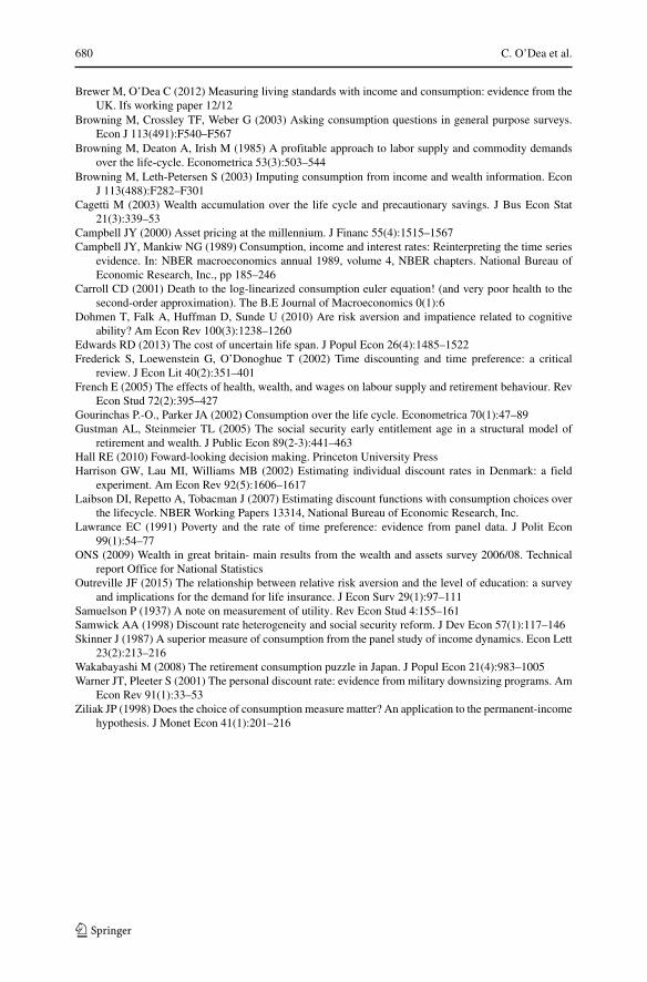
680 C. O’Dea et al.
Brewer M, O’Dea C (2012) Measuring living standards with income and consumption: evidence from theUK. Ifs working paper 12/12
Browning M, Crossley TF, Weber G (2003) Asking consumption questions in general purpose surveys.Econ J 113(491):F540–F567
Browning M, Deaton A, Irish M (1985) A profitable approach to labor supply and commodity demandsover the life-cycle. Econometrica 53(3):503–544
Browning M, Leth-Petersen S (2003) Imputing consumption from income and wealth information. EconJ 113(488):F282–F301
Cagetti M (2003) Wealth accumulation over the life cycle and precautionary savings. J Bus Econ Stat21(3):339–53
Campbell JY (2000) Asset pricing at the millennium. J Financ 55(4):1515–1567Campbell JY, Mankiw NG (1989) Consumption, income and interest rates: Reinterpreting the time series
evidence. In: NBER macroeconomics annual 1989, volume 4, NBER chapters. National Bureau ofEconomic Research, Inc., pp 185–246
Carroll CD (2001) Death to the log-linearized consumption euler equation! (and very poor health to thesecond-order approximation). The B.E Journal of Macroeconomics 0(1):6
Dohmen T, Falk A, Huffman D, Sunde U (2010) Are risk aversion and impatience related to cognitiveability? Am Econ Rev 100(3):1238–1260
Edwards RD (2013) The cost of uncertain life span. J Popul Econ 26(4):1485–1522Frederick S, Loewenstein G, O’Donoghue T (2002) Time discounting and time preference: a critical
review. J Econ Lit 40(2):351–401French E (2005) The effects of health, wealth, and wages on labour supply and retirement behaviour. Rev
Econ Stud 72(2):395–427Gourinchas P.-O., Parker JA (2002) Consumption over the life cycle. Econometrica 70(1):47–89Gustman AL, Steinmeier TL (2005) The social security early entitlement age in a structural model of
retirement and wealth. J Public Econ 89(2-3):441–463Hall RE (2010) Foward-looking decision making. Princeton University PressHarrison GW, Lau MI, Williams MB (2002) Estimating individual discount rates in Denmark: a field
experiment. Am Econ Rev 92(5):1606–1617Laibson DI, Repetto A, Tobacman J (2007) Estimating discount functions with consumption choices over
the lifecycle. NBER Working Papers 13314, National Bureau of Economic Research, Inc.Lawrance EC (1991) Poverty and the rate of time preference: evidence from panel data. J Polit Econ
99(1):54–77ONS (2009) Wealth in great britain- main results from the wealth and assets survey 2006/08. Technical
report Office for National StatisticsOutreville JF (2015) The relationship between relative risk aversion and the level of education: a survey
and implications for the demand for life insurance. J Econ Surv 29(1):97–111Samuelson P (1937) A note on measurement of utility. Rev Econ Stud 4:155–161Samwick AA (1998) Discount rate heterogeneity and social security reform. J Dev Econ 57(1):117–146Skinner J (1987) A superior measure of consumption from the panel study of income dynamics. Econ Lett
23(2):213–216Wakabayashi M (2008) The retirement consumption puzzle in Japan. J Popul Econ 21(4):983–1005Warner JT, Pleeter S (2001) The personal discount rate: evidence from military downsizing programs. Am
Econ Rev 91(1):33–53Ziliak JP (1998) Does the choice of consumption measure matter? An application to the permanent-income
hypothesis. J Monet Econ 41(1):201–216