direct torque control of permanent magnet
TRANSCRIPT

DIRECT TORQUE CONTROL OF PERMANENT MAGNET
SYNCHRONOUS MOTORS WITH NON-SINUSOIDAL BACK-EMF
A Dissertation
by
SALIH BARIS OZTURK
Submitted to the Office of Graduate Studies of Texas A&M University
in partial fulfillment of the requirements for the degree of
DOCTOR OF PHILOSOPHY
May 2008
Major Subject: Electrical Engineering

DIRECT TORQUE CONTROL OF PERMANENT MAGNET
SYNCHRONOUS MOTORS WITH NON-SINUSOIDAL BACK-EMF
A Dissertation
by
SALIH BARIS OZTURK
Submitted to the Office of Graduate Studies of Texas A&M University
in partial fulfillment of the requirements for the degree of
DOCTOR OF PHILOSOPHY
Approved by: Chair of Committee, Hamid A. Toliyat Committee Members, Prasat N. Enjeti S. P. Bhattacharyya Reza Langari Head of Department, Costas N. Georghiades
May 2008
Major Subject: Electrical Engineering

iii
ABSTRACT
Direct Torque Control of Permanent Magnet Synchronous Motors With Non-Sinusoidal
Back-EMF. (May 2008)
Salih Baris Ozturk, B.S., Istanbul Technical University, Istanbul, Turkey;
M.S., Texas A&M University, College Station
Chair of Advisory Committee: Dr. Hamid A. Toliyat
This work presents the direct torque control (DTC) techniques, implemented in
four- and six-switch inverter, for brushless dc (BLDC) motors with non-sinusoidal back-
EMF using two and three-phase conduction modes. First of all, the classical direct torque
control of permanent magnet synchronous motor (PMSM) with sinusoidal back-EMF is
discussed in detail. Secondly, the proposed two-phase conduction mode for DTC of
BLDC motors is introduced in the constant torque region. In this control scheme, only
two phases conduct at any instant of time using a six-switch inverter. By properly
selecting the inverter voltage space vectors of the two-phase conduction mode from a
simple look-up table the desired quasi-square wave current is obtained. Therefore, it is
possible to achieve DTC of a BLDC motor drive with faster torque response while the
stator flux linkage amplitude is deliberately kept almost constant by ignoring the flux
control in the constant torque region.
Third, the avarege current controlled boost power factor correction (PFC) method
is applied to the previously discussed proposed DTC of BLDC motor drive in the
constant torque region. The test results verify that the proposed PFC for DTC of BLDC

iv
motor drive improves the power factor from 0.77 to about 0.9997 irrespective of the
load.
Fourth, the DTC technique for BLDC motor using four-switch inverter in the
constant torque region is studied. For effective torque control in two phase conduction
mode, a novel switching pattern incorporating the voltage vector look-up table is
designed and implemented for four-switch inverter to produce the desired torque
characteristics. As a result, it is possible to achieve two-phase conduction DTC of a
BLDC motor drive using four-switch inverter with faster torque response due to the fact
that the voltage space vectors are directly controlled..
Finally, the position sensorless direct torque and indirect flux control (DTIFC) of
BLDC motor with non-sinusoidal back-EMF has been extensively investigated using
three-phase conduction scheme with six-switch inverter. In this work, a novel and simple
approach to achieve a low-frequency torque ripple-free direct torque control with
maximum efficiency based on dq reference frame similar to permanent magnet
synchronous motor (PMSM) drives is presented.

v
To my mother and father

vi
ACKNOWLEDGMENTS
This dissertation, while an induvidual work, would not be possible without the
kind assistance, encouragement and support of countless people, whom I want to thank.
I would like to thank, first and foremost, my advisor, Prof. Hamid A. Toliyat, for
his support, continuous help, patience, understanding and willingness throughout the
period of the research to which this dissertation relates. Moreover, spending his precious
time with me is appreciated far more than I have words to express. I am very grateful to
work with such a knowledgeable and insightful professor. Before pursuing graduate
education in the USA I spent a great amount of time finding a good school, and more
importantly a quality professor to work with. Even before working with Prof. Toliyat I
realized that the person you work with is more important than the prestige of the
university you attend. The education he provided me at Texas A&M University is
priceless.
I would also like to thank the members of my graduate study committee,
Prof. Prasad Enjeti, Prof. S.P. Bhattacharyya, and Prof. Reza Langari for accepting my
request to be a part of the committee even though they had a very busy schedule.
I would like to express my deepest gratitude to my fellow colleagues in the
Advanved Electric Machine and Power Electronics Laboratory: Dr. Bilal Akin, Dr.
Namhun Kim, Jeihoon Baek, Salman Talebi, Nicolas Frank, Steven Campbell, Anand
Balakrishnan, Robert Vartanian, Anil Chakali. I cherish their friendship and the good
memories I have had with them since my arrival at Texas A&M University.

vii
Also, I would like to thank to the people who are not participants of our lab but
who are my close friends and mentors who helped, guided, assisted and advised me
during the completion of this dissertation: Amir Toliyat, Dr. Oh Yang, David Tarbell,
and many others whom I may forget to mention here.
I would also like to acknowledge the Electrical Engineering department staff at
Texas A&M University: Ms. Tammy Carda, Ms. Linda Currin, Ms. Gayle Travis and
many others for providing an enjoyable and educational atmosphere.
Last but not least, I would like to thank my parents for their patience and endless
financial, and more importantly, moral support throughout my life. First, I am very
grateful to my dad for giving me the opportunity to study abroad to earn a good
education. Secondly, I am very grateful to my mother for her patience which gave me a
glimpse of how strong she is. Even though they do not show their emotion when I talk to
them, I can sense how much they miss me when I am away from them. No matter how
far away from home I am, they are always there to support and assist me. Finally, to my
parents, no words can express my gratitude for you and sacrifices you have made for me.

viii
TABLE OF CONTENTS
Page
ABSTRACT ...................................................................................................................... iii
DEDICATION ................................................................................................................... v
ACKNOWLEDGMENTS ................................................................................................. vi
TABLE OF CONTENTS ................................................................................................ viii
LIST OF FIGURES ........................................................................................................... xi
LIST OF TABLES ......................................................................................................... xvii
CHAPTER
I INTRODUCTION: DIRECT TORQUE CONTROL OF PERMANENT MAGNET SYNCHRONOUS MOTOR WITH SINUSOIDAL BACK-EMF .................................................................................................................. 1
1.1 Introduction and Literature Review ..................................................... 1 1.2 Principles of Classical DTC of PMSM Drive .................................... 11
1.2.1 Torque Control Strategy in DTC of PMSM Drive .............. 11 1.2.2 Flux Control Strategy in DTC of PMSM Drive .................. 16 1.2.3 Voltage Vector Selection in DTC of PMSM Drive ............ 19
1.3 Control Strategy of DTC of PMSM Drive ......................................... 24
II DIRECT TORQUE CONTROL OF BRUSHLESS DC MOTOR WITH NON-SINUSOIDAL BACK-EMF USING TWO-PHASE CONDUCTION MODE ................................................................................. 29
2.1 Introduction ........................................................................................ 29 2.2 Principles of the Proposed Direct Torque Control (DTC)
Technique ........................................................................................... 35 2.2.1 Control of Electromagnetic Torque by Selecting the
Proper Stator Voltage Space Vector ................................... 43 2.3 Simulation Results .............................................................................. 48 2.4 Experimental Results .......................................................................... 56 2.5 Conclusion .......................................................................................... 59

ix
CHAPTER Page
III POWER FACTOR CORRECTION OF DIRECT TORQUE CONTROLLED BRUSHLESS DC MOTOR WITH NON-SINUSOIDAL BACK-EMF USING TWO-PHASE CONDUCTION MODE ...................... 60
3.1 Introduction ........................................................................................ 60 3.2 The Average Current Control Boost PFC with Feed-Forward
Voltage Compensation ....................................................................... 63 3.2.1 Calculation of Feed-Forward Voltage Component C and
Multiplier Gain Km .............................................................. 64 3.3 Experimental Results .......................................................................... 67 3.4 Conclusion .......................................................................................... 74
IV DIRECT TORQUE CONTROL OF FOUR-SWITCH BRUSHLESS DC MOTOR WITH NON-SINUSOIDAL BACK-EMF USING TWO-PHASE CONDUCTION MODE ................................................................................. 75
4.1 Introduction ........................................................................................ 75 4.2 Topology of the Conventional Four-Switch Three-Phase AC Motor
Drive ................................................................................................... 78 4.2.1 Principles of the Conventional Four-Switch Inverter
Scheme ................................................................................ 78 4.2.2 Applicability of the Conventional Method to the BLDC
Motor Drive ......................................................................... 80 4.3 The Proposed Four-Switch Direct Torque Control of BLDC Motor
Drive ................................................................................................... 82 4.3.1 Principles of the Proposed Four-Switch Inverter Scheme .. 82 4.3.2 Control of Electromagnetic Torque by Selecting the
Proper Stator Voltage Space Vectors .................................. 88 4.3.3 Torque Control Strategies of the Uncontrolled Phase-c ...... 91
4.4 Simulation Results .............................................................................. 96 4.5 Experimental Results ........................................................................ 103 4.6 Conclusion ........................................................................................ 106
V SENSORLESS DIRECT TORQUE AND INDIRECT FLUX CONTROL OF BRUSHLESS DC MOTOR WITH NON-SINUSOIDAL BACK-EMF USING THREE-PHASE CONDUCTION MODE ...................................... 108
5.1 Introduction ...................................................................................... 108 5.2 The Proposed Line-to-Line Clarke and Park Transformations in
2x2 Matrix Form .............................................................................. 115 5.2.1 Conventional Park Transformation for Balanced
Systems ............................................................................. 115

x
CHAPTER Page
5.2.2 The Proposed Line-to-Line Clarke and Park Transformations for Balanced Systems ............................ 117
5.3 The Proposed Sensorless DTC of BLDC Drive Using Three-Phase Conduction .................................................................. 120 5.3.1 Principles of the Proposed Method ................................... 120 5.3.2 Electromagnetic Torque Estimation in dq and ba–ca
Reference Frames .............................................................. 127 5.3.3 Control of Stator Flux Linkage Amplitude ....................... 128 5.3.4 Control of Stator Flux Linkage Rotation and Voltage
Vector Selection for DTC of BLDC Motor Drive ............ 131 5.3.5 Estimation of Electrical Rotor Position ............................. 132
5.4 Simulation Results ............................................................................ 134 5.5 Experimental Results ........................................................................ 144 5.6 Conclusion ........................................................................................ 150
VI SUMMARY AND FUTURE WORK .......................................................... 152
REFERENCES ............................................................................................................... 157
APPENDIX A ................................................................................................................ 165
APPENDIX B ................................................................................................................ 167
APPENDIX C ................................................................................................................ 170
APPENDIX D ................................................................................................................ 172
APPENDIX E ................................................................................................................. 174
VITA .............................................................................................................................. 177

xi
LIST OF FIGURES
FIGURE Page
1.1. Eight possible voltage space vectors obtained from VSI ................................. 2 1.2. Circular trajectory of stator flux linkage in the stationary DQ−plane .............. 3 1.3. Phasor diagram of a non-saliet pole synchronous machine in the motoring mode ............................................................................................... 12 1.4. Electrical circuit diagram of a non-salient synchronous machine at constant frequency (speed) ............................................................................. 12 1.5. Rotor and stator flux linkage space vectors (rotor flux is lagging stator flux) ...................................................................................................... 15 1.6. Incremental stator flux linkage space vector representation in the DQ-plane ........................................................................................................ 16 1.7. Representation of direct and indirect components of the stator flux linkage vector ................................................................................................. 18 1.8. Voltage Source Inverter (VSI) connected to the R-L load ............................. 20 1.9. Voltage vector selection when the stator flux vector is located in sector i ............................................................................................................ 22 1.10. Basic block diagram for DTC of PMSM drive .............................................. 25 2.1. Actual (solid curved line) and ideal (straight dotted line) stator flux linkage trajectories, representation of two-phase voltage space vectors in the stationary αβ–axes reference frame ...................................................... 42 2.2. Representation of two-phase switching states of the inverter voltage space vectors for a BLDC motor .................................................................... 44 2.3. Overall block diagram of the two-phase conduction DTC of a BLDC motor drive in the constant torque region. ..................................................... 46

xii
FIGURE Page 2.4. Simulated open-loop stator flux linkage trajectory under the two-phase
conduction DTC of a BLDC motor drive at no load torque (speed + torque control) ........................................................................................................... 49
2.5. Simulated open-loop stator flux linkage trajectory under the two-phase conduction DTC of a BLDC motor drive at 1.2835 N·m load torque
(speed + torque control) ................................................................................. 50 2.6. Simulated phase–a voltage under 1.2 N·m load when zero voltage vector is used to decrease the torque (only torque control is performed) ................. 51 2.7. Simulated stator flux linkage locus with non-ideal trapezoidal back-EMF
under full load (speed + torque + flux control) .............................................. 52 2.8. Simulated phase–a current when flux control is obtained using (2.20) under full load (speed + torque + flux control) .............................................. 53 2.9. Simulated phase–a current when just torque is controlled without flux control under 1.2 N·m load with non-ideal trapezoidal back-EMF (reference torque is 1.225 N·m)...................................................................... 54 2.10. Simulated electromagnetic torque when just torque is controlled without flux control under 1.2 N·m load with non-ideal trapezoidal back-EMF
(reference torque is 1.225 N·m)...................................................................... 54 2.11. Simulated phase–a voltage when just torque is controlled without flux control under 1.2 N·m load with non-ideal trapezoidal back-EMF (reference torque is 1.225 N·m)...................................................................... 55 2.12. Experimental test-bed. (a) Inverter and DSP control unit. (b) BLDC motor
coupled to dynamometer and position encoder (2048 pulse/rev)................... 57 2.13. (a) Experimental phase–a current and (b) electromagnetic torque under
0.2292 N·m (0.2 pu) load ............................................................................... 58 3.1. Overall block diagram of the two-phase conduction DTC of a BLDC motor drive with boost PFC in the constant torque region ............................ 62 3.2. Experimental test-bed. (a) Inverter, DSP control unit, and boost PFC board. (b) BLDC motor coupled to dynamometer and position encoder (2048 pulse/rev.) ............................................................................................. 69

xiii
FIGURE Page 3.3. Measured steady-state phase–a current of two-phase DTC of BLDC motor
drive using boost PFC under 0.371 N·m load with 0.573 N·m reference torque. Current: 1.25 A/div. Time base: 7 ms/div .......................................... 70
3.4. Measured output dc voltage Vo, line voltage Vline, and line current Iline without PFC under no load with 0.4 N·m reference torque. (Top) Output dc voltage Vo = 80 V. (Middle) Line voltage Vline = 64.53 Vrms. (Bottom) Line current Iline = 1.122 A. Vo: 20 V/div; Iline: 2 A/div; Vline: 50 V/div. Time base: 5 ms/div ............................................................... 71 3.5. Measured steady-state output dc voltage Vo, line voltage Vline, and line current Iline with PFC under no load with 0.4 N·m reference torque. (Top)
Output dc voltage Vo = 80 V. (Middle) Line voltage Vline = 25.43 Vrms. (Bottom) Line current Iline = 2.725 A. Vo: 20 V/div; Iline: 5 A/div;
Vline: 50 V/div. Time base: 5 ms/div ............................................................... 72 3.6. Measured steady-state output dc voltage Vo, line voltage Vline, and line current Iline with PFC under 0.371 N·m load torque with 0.573 N·m reference torque. (Top) Output dc voltage Vo = 80 V. (Middle) Line voltage Vline = 25.2 Vrms. (Bottom) Line current Iline = 4.311 A. Vo: 20 V/div; Iline: 5 A/div; Vline: 50 V/div. Time base: 5 ms/div ................... 73 4.1. Conventional four-switch voltage vector topology. (a) (0,0) vector, (b) (1,1) vector, (c) (1,0) vector, and (d) (0,1) vector .................................... 79 4.2. Actual (realistic) phase back-EMF, current, and phase torque profiles of the three-phase BLDC motor drive with four-switch inverter ................... 81 4.3. Actual (solid curved lines) and ideal (straight dotted lines) stator flux linkage trajectories, representation of the four-switch two-phase voltage
space vectors, and placement of the three hall-effect sensors in the stationary αβ–axes reference frame (Vdc_link = Vdc) ........................................ 86 4.4. Representation of two-phase switching states of the four-switch inverter
voltage space vectors for a BLDC motor ....................................................... 86 4.5. Proposed four-switch voltage vector topology for two-phase conduction DTC of BLDC motor drives. (a) V1(1000) vector, (b) V2(0010) vector, (c) V3(0110) vector, (d) V4(0100) vector, (e) V5(0001) vector, (f) V6(1001), (g) V7(0101), and (h) V0(1010) ................................................ 87

xiv
FIGURE Page 4.6. Individual phase–a and –b torque control, Tea and Teb , in Sectors 2 and 5 ............................................................................................................... 93 4.7. Overall block diagram of the four-switch two-phase conduction DTC of a BLDC motor drive in the constant torque region .................................... 94
4.8. Simulated open-loop stator flux linkage trajectory under the four-switch two-phase conduction DTC of a BLDC motor drive at no load torque (speed + torque control) ................................................................................. 98 4.9. Simulated open-loop stator flux linkage trajectory under the four-switch two-phase conduction DTC of a BLDC motor drive at 1.2835 N·m load
torque (speed + torque control) ...................................................................... 98 4.10. Simulated stator flux linkage locus whose reference is chosen from (4.3) under full load (speed + torque + flux control) .............................................. 99 4.11. Simulated electromagnetic torque using actual αβ–axes motor back-EMFs
under full load (speed + torque + flux control) .............................................. 99 4.12. Simulated abc frame phase currents when stator flux reference is obtained
from (4.3) under full load (speed + torque + flux control) ........................... 101 4.13. Simulated abc frame phase currents when just torque is controlled without
flux control under 0.5 N·m load using actual back-EMFs (reference torque is 0.51 N·m) ....................................................................................... 102 4.14. Simulated electromagnetic torque when just torque is controlled without flux control under 0.5 N·m load using actual back-EMFs (reference torque is 0.51 N·m) ....................................................................................... 103 4.15. Experimental test-bed. (a) Four-switch inverter and DSP control unit. (b) BLDC motor coupled to dynamometer and position encoder (2048
pulse/rev) ...................................................................................................... 104 4.16. Top: Steady-state and transient experimental electromagnetic torque in per-unit under 0.5 N·m load torque (0.5 N·m/div). Bottom: Steady-state and transient experimental abc frame phase currents (2 A/div) and time base: 16.07 ms/div ........................................................................................ 106 5.1. Rotor and stator flux linkages of a BLDC motor in the stationary αβ–plane and synchronous dq–plane ........................................................... 125
xv
FIGURE Page 5.2. Decagon trajectory of stator flux linkage in the stationary αβ–plane .......... 131 5.3. BLDC motor stator flux linkage estimation with an amplitude limiter ....... 134 5.4. Overall block diagram of the sensorless direct torque and indirect flux control of BLDC motor drive using three-phase conduction mode ............. 135 5.5. Simulated indirectly controlled stator flux linkage trajectory under the sensorless three-phase conduction DTC of a BLDC motor drive at 0.5 N·m load torque (ids
r* = 0) ...................................................................... 136 5.6. Simulated indirectly controlled stator flux linkage trajectory under the sensorless three-phase conduction DTC of a BLDC motor drive when ids
r is changed from 0 A to -5 A at 0.5 N·m load torque .................................... 137 5.7. Steady-state and transient behavior of (a) simulated ba–ca frame currents, (b) actual electromagnetic torque, and (c) estimated electromagnetic torque under 0.5 N·m load torque................................................................. 138 5.8. Steady-state and transient behavior of (a) estimated electrical rotor position, (b) actual electrical rotor position under 0.5 N·m load torque ...... 141 5.9. Actual ba–ca frame back-EMF constants versus electrical rotor position
( ( )ba ek θ and ( )ca ek θ ) .................................................................................... 142 5.10. Actual q– and d–axis rotor reference frame back-EMF constants versus
electrical rotor position ( ( )q ek θ and ( )d ek θ ) ................................................ 143 5.11. Steady-state and transient behavior of the simulated q– and d–axis rotor
reference frame currents when idsr*= 0 under 0.5 N·m load torque .............. 143
5.12. Experimental test-bed. (a) Inverter and DSP control unit. (b) BLDC motor coupled to dynamometer and position encoder is not used ............... 145 5.13. Steady-state and transient behavior of the experimental (a) ba–ca frame
currents, and (b) estimated electromagnetic torque under 0.5 N·m load torque. ................................................................................................... 146 5.14. Experimental indirectly controlled stator flux linkage trajectory under the sensorless three-phase conduction DTC of a BLDC motor drive when ids
r*= 0 at 0.5 N·m load torque. ..................................................................... 148

xvi
FIGURE Page 5.15. Steady-state and transient behavior of the experimental q– and d–axis rotor reference frame currents when ids
r*= 0 under 0.5 N·m load torque. .... 148 5.16. Steady-state and transient behavior of the actual and estimated electrical rotor positions from top to bottom under 0.5 N·m load torque. ................... 149 A.1. (a) Actual line-to-line back-EMF constants (kab(θe), kbc(θe) and kca(θe)) and (b) stationary reference frame back-EMF constants (kα(θe)and kβ(θe)) . 165 E.1. Line-to-line back-EMF waveforms (eab, ebc, and eca) .................................. 174 E.2. α–axis back-EMF (eα) waveform ................................................................. 176

xvii
LIST OF TABLES
TABLE Page
I Switching Table for DTC of PMSM Drive .................................................... 23
II Two-phase Voltage Vector Selection for BLDC Motor ................................ 43
III Electromagnetic Torque Equations for the Operating Regions ..................... 84
IV Two-Phase Four-Switch Voltage Vector Selection for DTC of BLDC Motor Drive (CCW) ....................................................................................... 89
V Voltage Vector Selection in Sectors II and V for Four-Switch DTC of BLDC Motor Drive (CCW) ........................................................................... 89
VI Switching Table for DTC of BLDC Motor Using Three-Phase Conduction ................................................................................................... 132

1
CHAPTER I
INTRODUCTION: DIRECT TORQUE CONTROL OF PERMANENT
MAGNET SYNCHRONOUS MOTOR WITH SINUSOIDAL BACK-EMF
1.1. Introduction and Literature Review
Today there are basically two types of instantaneous electromagnetic torque-
controlled ac drives used for high-performance applications: vector and direct torque
control (DTC) drives. The most popular method, vector control was introduced more
than 25 years ago in Germany by Hasse [1], Blaske [2], and Leonhard. The vector
control method, also called Field Oriented Control (FOC) transforms the motor
equations into a coordinate system that rotates in synchronism with the rotor flux vector.
Under a constant rotor flux amplitude there is a linear relationship between the control
variables and the torque. Transforming the ac motor equations into field coordinates
makes the FOC method resemble the decoupled torque production in a separately
excited dc motor. Over the years, FOC drives have achieved a high degree of maturity in
a wide range of applications. They have established a substantial worldwide market
which continues to increase [3].
No later than 20 years ago, when there was still a trend toward standardization of
control systems based on the FOC method, direct torque control was introduced in Japan
____________________
This dissertation follows the style and format of IEEE Transactions on Industry Applications.
2
by Takahashi and Nagochi [4] and also in Germany by Depenbrock [5], [6], [7]. Their
innovative studies depart from the idea of coordinate transformation and the analogy
with dc motor control. These innovators proposed a method that relies on a bang-bang
control instead of a decoupling control which is the characteristic of vector control.
Their technique (bang-bang control) works very well with the on-off operation of
inverter semiconductor power devices.
After the innovation of the DTC method it has gained much momentum, but in
areas of research. So far only one form of a DTC of ac drive has been marketed by an
industrial company, but it is expected very soon that other manufacturers will come out
with their own DTC drive products [8].
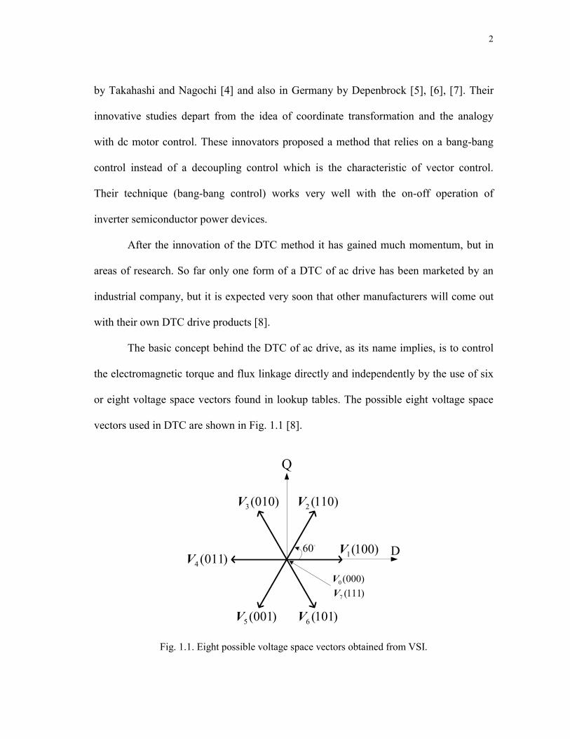
The basic concept behind the DTC of ac drive, as its name implies, is to control
the electromagnetic torque and flux linkage directly and independently by the use of six
or eight voltage space vectors found in lookup tables. The possible eight voltage space
vectors used in DTC are shown in Fig. 1.1 [8].
D
Q
60
6 (101)V
1(100)V
2 (110)V3 (010)V
4 (011)V
5 (001)V
0 (000)V
7 (111)V
Fig. 1.1. Eight possible voltage space vectors obtained from VSI.

3
The typical DTC includes two hysteresis controllers, one for torque error
correction and one for flux linkage error correction. The hysteresis flux controller makes
the stator flux rotate in a circular fashion along the reference trajectory for sinewave ac
machines as shown in Fig. 1.2. The hysteresis torque controller tries to keep the motor
torque within a pre-defined hysteresis band.
D
Q
2θ
1θ
6θ5
V6
V
3V
2V
4V1
V
1V
2V3V
1V
2V
3V4
V3
V4V
5V
4V
5V
6V
5V
6V
6V1V
2V
3θ
4θ
5θ
Fig. 1.2. Circular trajectory of stator flux linkage in the stationary DQ−plane.
At every sampling time the voltage vector selection block decides on one of the
six possible inverter switching states ( aS , bS , cS ) to be applied to the motor terminals.
The possible outputs of the hysteresis controller and the possible number of switching
states in the inverter are finite, so a look-up table can be constructed to choose the

4
appropriate switching state of the inverter. This selection is a result of both the outputs
of the hysteresis controllers and the sector of the stator flux vector in the circular
trajectory.
There are many advantages of direct torque control over other high-performance
torque control systems such as vector control. Some of these are summarized as follows:
• The only parameter that is required is stator resistance
• The switching commands of the inverter are derived from a look-up table,
simplifying the control system and also decreasing the processing time unlike a
PWM modulator used in vector control
• Instead of current control loops, stator flux linkage vector and torque estimation
are required so that simple hysteresis controllers are used for torque and stator
flux linkage control
• Vector transformation is not applied because stator quantities are enough to
calculate the torque and stator flux linkage as feedback quantities to be compared
with the reference values
• The rotor position, which is essential for torque control in a vector control
scheme, is not required in DTC (for induction and synchronous reluctance motor
DTC drives)
Once the initial position of the rotor magnetic flux problem is solved for PMSM
drives by some initial rotor position estimation techniques or by bringing the rotor to the
known position, DTC of the PMSM can be as attractive as DTC of an induction motor. It
is also easier to implement and as cost-effective (no position sensor is required) when

5
compared to vector controlled PMSM drives. The DTC scheme, as its name indicates, is
focused on the control of the torque and the stator flux linkage of the motor, therefore, a
faster torque response is achieved over vector control. Furthermore, due to the fact that
DTC does not need current controller, the time delay caused by the current loop is
eliminated.
Even though the DTC technique was originally proposed for the induction
machine drive in the late 1980’s, its concept has been extended to the other types of ac
machine drives recently, such as switched reluctance and synchronous reluctance
machines. In the late 90s, DTC techniques for the interior permanent magnet
synchronous machine appeared, as reported in [9], [10].
Although there are several advantages of the DTC scheme over vector control, it
still has a few drawbacks which are explained below:
• A major drawback of the DTC scheme is the high torque and stator flux linkage
ripples. Since the switching state of the inverter is updated once every sampling
time, the inverter keeps the same state until the outputs of each hysteresis
controller changes states. As a result, large ripples in torque and stator flux
linkage occur.
• The switching frequency varies with load torque, rotor speed and the bandwidth
of the two hysteresis controllers.
• Stator flux estimation is achieved by integrating the difference between the input
voltage and the voltage drop across the stator resistance (by the back-EMF
integration as given in (1.9)). The applied voltage on the motor terminal can be

6
obtained either by using a dc-link voltage sensor, or two voltage sensors
connected to the any two phases of the motor terminals. For current sensing there
should be two current sensors connected on any two phases of the motor
terminals. Offset in the measurements of dc-link voltage and the stator currents
might happen, because for current and voltage sensing, however, temperature
sensitive devices, such as operational amplifiers, are normally used which can
introduce an unwanted dc offset. This offset may introduce large drifts in the
stator flux linkage computation (estimation) thus creating an error in torque
estimation (torque is proportional to the flux value) which can make the system
become unstable.
• The stator flux linkage estimation has a stator resistance, so any variation in the
stator resistance introduces error in the stator flux linkage computation,
especially at low frequencies. If the magnitude of the applied voltage and back-
EMF are low, then any change in the resistance will greatly affect the integration
of the back-EMF.
• Because of the constant energy provided from the permanent magnet on the rotor
the rotor position of motor will not necessarily be zero at start up. To
successfully start the motor under the DTC scheme from any position (without
locking the motor at a known position), the initial position of the rotor magnetic
flux must be known. Once it is started properly, however, the complete DTC
scheme does not explicitly require a position sensor.

7
From the time the DTC scheme was discovered for ac motor drives, it was
always inferior to vector control because of the disadvantages associated with it. The
goal is to bring this technology as close to the performance level of vector control and
even exceed it while keeping its simple control strategy and cost-effectiveness. As a
result, many papers have been presented by several researchers to minimize or overcome
the drawbacks of the DTC scheme. Here are some of the works that have been done by
researchers to overcome the drawbacks for the most recent ac drive technology using
direct torque control:
• Recently, researchers have been working on the torque and flux ripple reduction,
and fixing the switching frequency of the DTC system, as reported in [11]–[16].
Additionally, they came up with a multilevel inverter solution in which there are
more voltage space vectors available to control the flux and torque. As a
consequence, smoother torque can be obtained, as reported in [14] and [15], but
by doing so, more power switches are required to achieve a lower ripple and an
almost fixed switching frequency, which increases the system cost and
complexity. In the literature, a modified DTC scheme with fixed switching
frequency and low torque and flux ripple was introduced in [13] and [16]. With
this design, however, two PI regulators are required to control the flux and torque
and they need to be tuned properly. Very recently Rahman [17] proposed a
method for torque and flux ripple reduction in interior permanent magnet
synchronous machines under an almost fixed switching frequency without using

8
any additional regulators. This method is a modified version of the previously
discovered method for the induction machine by the authors in [18].
• Stator flux linkage estimation by the integration of the back-EMF should be reset
regularly to reduce the effect of the dc offset error. There has been a few
compensation techniques related to this phenomenon proposed in the literature
[19]–[21] and [22]. Chapuis et al. [19] introduced a technique to eliminate the dc
offset, but a constant level of dc offset is assumed which is usually not the case.
In papers [19]–[21] and [22], low-pass filters (LPFs) have been introduced to
estimate the stator flux linkage. In [19], a programmable cascaded LPF was
proposed instead of the single-stage integrator to help decrease the dc offset error
more than the single-stage integrator for induction motor drives. More recently,
Rahman [23] has reached an approach like [19] with further investigation and
implementation for the compensation of dc offset error in a direct controlled
interior permanent magnet (IPM) synchronous motor drive. It has been claimed
and proven with simulation and experimental results that programmable cascaded
LPFs can also be adopted to replace the single-stage integrator and compensate
for the effect of dc offsets in a direct-torque-controlled IPM synchronous motor
drive, improving the performance of the drive.
• The voltage drop in the stator resistance is very large when the motor runs at low
frequency such that any small deviations in stator resistance from the one used in
the estimation of the stator flux linkage creates large errors between the reference
and actual stator flux linkage vector. This also affects the torque estimation as

9
well. Due to these errors, the drive can easily go unstable when operating at low
speeds. The worst case scenario might happen at low speed under a very high
load. A handful of researchers have recently pointed to the issue of stator
resistance variation for the induction machine. For example, fuzzy and
proportional-integral (PI) stator resistance estimators have been developed and
compared for a DTC induction machine based on the error between the reference
current and the actual one by Mir et al. [24]. On the other hand, they did not
show any detail on how to obtain the reference current for the stator resistance
estimation. Additionally, some stability problems of the fuzzy estimator were
observed when the torque reference value was small. As reported in [25], fuzzy
logic based stator resistance observers are introduced for induction motor. Even
though it is an open-loop controller based on fuzzy rules, the accuracy of
estimating the stator resistance is about 5% and many fuzzy rules are necessary.
This resulted in having to conduct handful numbers of extensive experiments to
create the fuzzy rules resulting in difficulty in implementation. Lee and Krishnan
[26] contributed a work related to the stator resistance estimation of the DTC
induction motor drive by a PI regulator. An instability issue caused by the stator
estimation error in the stator resistance, the mathematical relationships between
stator current, torque and flux commands, and the machine parameters are also
analyzed in their work. The stator configuration of all ac machines is almost the
same, so the stator resistance variation problem still exists for permanent magnet
synchronous motors. Rahman et al. [27] reported a method, for stator resistance

10
estimation by PI regulation based on the error in flux linkage. It is claimed that
any variation in the stator resistance of the PM synchronous machine will cause a
change in the amplitude of the actual flux linkage. A PI controller works in
parallel with the hysteresis flux controller of the DTC such that it tracks the
stator resistance by eliminating the error in the command and the actual flux
linkage. One problem with this method was that the rotor position was necessary
to calculate the flux linkage. Later on the same author proposed a similar method
but this time the PI stator resistance estimator was able to track the change of the
stator resistance without requiring any position information.
• The back-EMF integration for the stator flux linkage calculation, which runs
continuously, requires a knowledge of the initial stator flux position, 0tsλ =, at
start up. In order to start the motor without going in the wrong direction,
assuming the stator current is zero at the start, only the rotor magnetic flux
linkage should be considered as an initial flux linkage value in the integration
formula. The next step is to find its position in the circular trajectory. The initial
position of the rotor is not desired to be sensed by position sensors due to their
cost and bulky characteristics, therefore some sort of initial position sensing
methods are required for permanent magnet synchronous motor DTC
applications. A number of works, [28]–[39], have been proposed recently for the
detection of the initial rotor position estimation at standstill for different types of
PM motors. Common problems of these methods include: most of them fail at
standstill because the rotor magnet does not induce any voltage, so no

11
information of the magnetization is available; position estimation is load
dependent; excessive computation and hardware are required; instead of a simple
voltage vector selection method used in the DTC scheme, those estimation
techniques need one or more pulse width-modulation (PWM) current controllers.
Recently, a better solution was introduced for the rotor position estimation. It is
accomplished by applying high-frequency voltage to the motor, as reported in
[37]–[39]. This approach is adapted to the DTC of interior permanent magnet
motors for initial position estimation by Rahman et. al. [23].
1.2. Principles of Classical DTC of PMSM Drive
The basic idea of direct torque control is to choose the appropriate stator voltage
vector out of eight possible inverter states (according to the difference between the
reference and actual torque and flux linkage) so that the stator flux linkage vector rotates
along the stator reference frame (DQ frame) trajectory and produces the desired torque.
The torque control strategy in the direct torque control of a PM synchronous motor is
explained in Section 1.2.1. The flux control is discussed following the torque control
section.
1.2.1. Torque Control Strategy in DTC of PMSM Drive
Before going through the control principles of DTC for PMSMs, an expression
for the torque as a function of the stator and rotor flux will be developed. The torque
equation used for DTC of PMSM drives can be derived from the phasor diagram of
permanent magnet synchronous motor shown in Fig. 1.3.

12
δ
d-axis
q-axis
s sI R
E
s sjI X
sV
sIϕ
rλ
Fig. 1.3. Phasor diagram of a non-salient pole synchronous machine in the motoring mode.
R ss LjjX ω=
°∠0V °∠δfE
Fig. 1.4. Electrical circuit diagram of a non-salient synchronous machine at constant frequency
(speed).
When the machine is loaded through the shaft, the motor will take real power.
The rotor will then fall behind the stator rotating field. From the circuit diagram, shown
in Fig. 1.4, the motor current expression can be written as

13
0 0s ss
s s s
V E V EIR jX Z
δ δϕ
∠ − ∠ ∠ − ∠= =
+ ∠ (1.1)
where 2 2s s sZ R X= + , also s e sX Lω=
and 1tan s
s
XR
ϕ −⎛ ⎞⎟⎜ ⎟= ⎜ ⎟⎜ ⎟⎜⎝ ⎠
Assuming a reasonable speed such that the sX term is higher than the resistance
sR such that sR can be neglected, then s sZ X≈ and 2π
ϕ≈ . sI can then be rewritten as
0 2ss
s s
EVIX X
πδ∠ −∠= −
(1.2)
Such that the real part of sI is
Re[ ] cos cos cos
2 2
cos sin2
ss s
s s
s s
V EI IX X
E EX X
π πϕ δ
πδ δ
⎛ ⎞ ⎛ ⎞⎟ ⎟⎜ ⎜= = − − −⎟ ⎟⎜ ⎜⎟ ⎟⎜ ⎜⎝ ⎠ ⎝ ⎠
⎛ ⎞⎟⎜=− − =−⎟⎜ ⎟⎜⎝ ⎠
(1.3)
The developed power is given by
3 Re[ ] 3 cosi s s s sP V I V I ϕ= = (1.4)
Substituting (1.3) into (1.4) yields
3 sinsi
s
V EPX
δ=− [Watts/phase] (1.5)
This power is positive when δ negative, meaning that when the rotor field lags
the stator field the machine is operating in the motoring region. When 0δ> the machine
is operating in the generation region. The negative sign in (1.5) can be dropped,
assuming that for motoring operation a negative δ is implied.

14
If the losses of the machine are ignored, the power iP can be expressed as the
shaft (output) power as well
2i o e emP P T
Pω= = (1.6)
When combining (1.5) and (1.6), the magnitude of the developed torque for a
non-salient synchronous motor (or surface-mounted permanent magnet synchronous
motor) can be expressed as
3 sin
2
3 sin2
eme s
s
PTX
PL
δω
δ
⎛ ⎞⎟⎜= ⎟⎜ ⎟⎜⎝ ⎠
⎛ ⎞⎟⎜= ⎟⎜ ⎟⎜⎝ ⎠
s
s r
V E
λ λ (1.7)
where δ is the torque angle between flux vectors sλ and rλ . If the rotor flux remains
constant and the stator flux is changed incrementally by the stator voltage sV then the
torque variation emTΔ expression can be written as
3 sin2em
s
PTL
δ⎛ ⎞ +⎟⎜Δ = Δ⎟⎜ ⎟⎜⎝ ⎠
s s rλ Δλ λ (1.8)
where the bold terms in the above expressions indicate vectors.
As it can be seen from (1.8), if the load angle δ is increased then torque variation
is increased. To increase the load angle δ the stator flux vector should turn faster than
rotor flux vector. The rotor flux rotation depends on the mechanical speed of the rotor,
so to decrease load angle δ the stator flux should turn slower than rotor flux. Therefore,
according to the torque (1.7), the electromagnetic torque can be controlled effectively by
controlling the amplitude and rotational speed of stator flux vector sλ . To achieve the

15
above phenomenon, appropriate voltage vectors are applied to the motor terminals. For
counter-clockwise operation, if the actual torque is smaller than the reference value, then
the voltage vectors that keep the stator flux vector sλ rotating in the same direction are
selected. When the load angle δ between sλ and rλ increases the actual torque increases
as well. Once the actual torque is greater than the reference value, the voltage vectors
that keep stator flux vector sλ rotating in the reverse direction are selected instead of the
zero voltage vectors. At the same time, the load angle δ decreases thus the torque
decreases. The reason the zero voltage vector is not chosen in the DTC of PMSM drives
will be discussed later in this chapter. A more detailed look at the selection of the
voltage vectors and their effect on torque and flux results will be discussed later as well.
Referring back to the discussion above, however, torque is controlled via the stator flux
rotation speed, as shown in Fig. 1.5. If the speed of the stator flux is high then faster
torque response is achieved.
reωsω
δ
sλ
rλ
Im
Rereθsθ
Fig. 1.5. Rotor and stator flux linkage space vectors (rotor flux lagging stator flux) [21].

16
1.2.2. Flux Control Strategy in DTC of PMSM Drive
If the resistance term in the stator flux estimation algorithm is neglected, the
variation of the stator flux linkage (incremental flux expression vector) will only depend
on the applied voltage vector as shown in Fig. 1.6 [40].
D
Q
2θ
1θ
6θ
3θ
4θ
5θ
0sλ
sλ∗
2Hλ
3V
2V
4V
3V4V
5V4V
5V
6V
5V
6V
1V6V
1V
2V
2V
2V3V
4V
5V 6V
1V
sλ
2 sV T
3V
Fig. 1.6. Incremental stator flux linkage space vector representation in the DQ−plane.
For a short interval of time, namely the sampling time sT t=Δ the stator flux
linkage sλ position and amplitude can be changed incrementally by applying the stator
voltage vector sV . As discussed above, the position change of the stator flux linkage
vector sλ will affect the torque. The stator flux linkage of a PMSM that is depicted in
the stationary reference frame is written as
( )s s s sR dt= −∫λ V i (1.9)

17
During the sampling interval time or switching interval, one out of the six
voltage vectors is applied, and each voltage vector applied during the pre-defined
sampling interval is constant, therefore (1.9) can be rewritten as
s s s s s t=0t - R dt + λ= ∫λ V i (1.10)
where s t=0λ is the initial stator flux linkage at the instant of switching, Vs is the
measured stator voltage, is is the measured stator current, and sR is the estimated stator
resistance. When the stator term in stator flux estimation is removed implying that the
end of the stator flux vector sλ will move in the direction of the applied voltage vector,
as shown in Fig. 1.6, we obtain
( )V λs sddt
= (1.11)
or
Δts sΔλ =V (1.12)
The goal of controlling the flux in DTC is to keep its amplitude within a pre-
defined hysteresis band. By applying a required voltage vector stator flux linkage
amplitude can be controlled. To select the voltage vectors for controlling the amplitude
of the stator flux linkage the voltage plane is divided into six regions, as shown in Fig.
1.2.
In each region two adjacent voltage vectors, which give the minimum switching
frequency, are selected to increase or decrease the amplitude of stator flux linkage,
respectively. For example, according to the Table I, when the voltage vector 2V is
applied in Sector 1, then the amplitude of the stator flux increases when the flux vector

18
rotates counter-clockwise. If 3V is selected then stator flux linkage amplitude decreases.
The stator flux incremental vectors corresponding to each of the six inverter voltage
vectors are shown in Fig. 1.1.
sω
s sTω
sλ
0sλ
Im
Re0sθ
sθ
s sV T
Direct (Flux) component
Indirect (Torque) component
Fig. 1.7. Representation of direct and indirect components of the stator flux linkage vector [21].
Fig. 1.7 is a basic graph that shows how flux and torque can be changed as a
function of the applied voltage vector. According to the figure, the direct component of
applied voltage vector changes the amplitude of the stator flux linkage and the indirect
component changes the flux rotation speed which changes the torque. If the torque needs
to be changed abruptly then the flux does as well, so the closest voltage vector to the
indirect component vector is applied. If torque change is not required, but flux amplitude
is increased or decreased then the voltage vector closest to the direct component vector
is chosen. Consequently, if both torque and flux are required to change then the
appropriate resultant mid-way voltage vector between the indirect and direct components
is applied [21]. It seems obvious from (1.9) that the stator flux linkage vector will stay at
its original position when zero voltage vectors (000)aS and (111)aS are applied. This is

19
true for an induction motor since the stator flux linkage is uniquely determined by the
stator voltage. On the other hand, in the DTC of a PMSM, the situation of applying the
zero voltage vectors is not the same as in induction motors. This is because the stator
flux linkage vector will change even when the zero voltage vectors are selected since the
magnets rotate with the rotor. As a result, the zero voltage vectors are not used for
controlling the stator flux linkage vector in a PMSM. In other words, the stator flux
linkage should always be in motion with respect to the rotor flux linkage vector [10].
1.2.3. Voltage Vector Selection in DTC of PMSM Drive
As discussed before, the stator flux is controlled by properly selected voltage
vectors, and as a result the torque by stator flux rotation. The higher the stator vector
rotation speed the faster torque response is achieved.
The estimation of the stator flux linkage components described previously
requires the stator terminal voltages. In a DTC scheme it is possible to reconstruct those
voltages from the dc-link voltage dcV and the switching states ( aS , bS , cS ) of a six-step
voltage-source inverter (VSI) rather than monitoring them from the motor terminals. The
primary voltage vector sv is defined by the following equation:
(2 /3) (4 /3)2 ( )3
j js a b cv v e v eπ π= + +v (1.13)
where av , bv , and cv are the instantaneous values of the primary line-to-neutral voltages.
When the primary windings are fed by an inverter, as shown in Fig. 1.8, the primary
voltages av , bv and cv are determined by the status of the three switches aS , bS , and

20
cS . If the switch is at state 0 that means the phase is connected to the negative and if it is
at 1 it means that the phase is connected to the positive leg.
aS bS cS1
0
1
0
1
0
dcV
D
Q
Fig. 1.8. Voltage Source Inverter (VSI) connected to the R-L load [5].
For example, av is connected to dcV if aS is one, otherwise av is connected to
zero. This is similar for bv and cv . The voltage vectors that are obtained this way are
shown in Fig. 1.1. There are six nonzero voltage vectors: 1(100)V , 2 (110)V , …, and
6 (101)V and two zero voltage vectors: 7 (000)V and 8 (111)V . The six nonzero voltage
vectors are 60 apart from each other as in Fig. 1.1.
The stator voltage space vector (expressed in the stationary reference frame)
representing the eight voltage vectors can be shown by using the switching states and the
dc-link voltage dcV as
(2/ 3) (4 /3)2( , , ) ( )
3j j
s a b c dc a b cS S S V S S e S eπ π= + +v (1.14)
where dcV is the dc-link voltage and the coefficient of 2/3 is the coefficient comes from
the Park Transformation. Equation (1.14) can be derived by using the line-to-line

21
voltages of the ac motor which can be expressed as ( )ab dc a bv V S S= − ,
( )bc dc b cv V S S= − , and ( )ca dc c av V S S= − . The stator phase voltages (line-to-neutral
voltages) are required for (1.14). They can be obtained from the line-to-line voltages as
( ) / 3a ab cav v v= − , ( ) / 3b bc abv v v= − , and ( ) / 3c ca bcv v v= − . If the line-to-line voltages
in terms of the dc-link voltage dcV and switching states are substituted into the stator
phase voltages it gives
1 (2 )3a dc a b cv V S S S= − −
1 ( 2 )3b dc a b cv V S S S= − + − (1.15)
1 ( 2 )3c dc a b cv V S S S= − − +
Equation (1.15) can be summarized by combining with (1.13) as
1Re( ) (2 )3a s dc a b cv V S S S= = − −v
1Re( ) ( 2 )3b s dc a b cv V S S S= = − + −v (1.16)
1Re( ) ( 2 )3c s dc a b cv V S S S= = − − +v
To determine the proper applied voltage vectors, information from the torque and
flux hysteresis outputs, as well as stator flux vector position, are used so that circular
stator flux vector trajectory is divided into six symmetrical sections according to the non
zero voltage vectors as shown in Fig. 1.2.

22
iV
1iV +2iV +
1iV −2iV −
3iV +
sλ
D
Q
2θ
1θ
6θ
emTsλ
emTsλ
emTsλ
emTsλ
Fig. 1.9. Voltage vector selection when the stator flux vector is located in sector i [21].
According to Fig. 1.9, while the stator flux vector is situated in sector i, voltage
vectors i+1V and i-1V have positive direct components, increasing the stator flux
amplitude, and i+2V and i-2V have negative direct components, decreasing the stator flux
amplitude. Moreover, i+1V and i+2V have positive indirect components, increasing the
torque response, and i-1V and i-2V have negative indirect components, decreasing the
torque response. In other words, applying i+1V increases both torque and flux but
applying i+1V increases torque and decreases flux amplitude [21].
The switching table for controlling both the amplitude and rotating direction of
the stator flux linkage is given in Table I.

23
TABLE I SWITCHING TABLE FOR DTC OF PMSM DRIVE
V2(110) V3(010) V4(001) V5(101) V6(110) V1(110)V6(101) V1(100) V2(010) V3(011) V4(110) V5(110)V3(010) V4(011) V5(101) V6(100) V1(110) V2(110)V5(001) V6(101) V1(110) V2(010) V3(110) V4(110)
θθ(1) θ(2) θ(3) θ(4) θ(5) θ(6)
ϕ τ
1ϕ=
0ϕ=
1τ =0τ =1τ =0τ =
The voltage vector plane is divided into six sectors so that each voltage vector
divides each region into two equal parts. In each sector, four of the six non-zero voltage
vectors may be used. Zero vectors are also allowed. All the possibilities can be tabulated
into a switching table. The switching table presented by Rahman et al [10] is shown in
Table I. The output of the torque hysteresis comparator is denoted as τ , the output of the
flux hysteresis comparator as ϕ and the flux linkage sector is denoted as θ . The torque
hysteresis comparator is a two valued comparator; 0τ = means that the actual value of
the torque is above the reference and out of the hysteresis limit and 1=τ means that the
actual value is below the reference and out of the hysteresis limit. The flux hysteresis
comparator is a two valued comparator as well where 1ϕ = means that the actual value
of the flux linkage is below the reference and out of the hysteresis limit and 0ϕ=
means that the actual value of the flux linkage is above the reference and out of the
hysteresis limit. Rahman et al [10] have suggested that no zero vectors should be used
with a PMSM. Instead, a non zero vector which decreases the absolute value of the
torque is used. Their argument was that the application of a zero vector would make the
change in torque subject to the rotor mechanical time constant which may be rather long

24
compared to the electrical time constants of the system. This results in a slow change of
the torque. This reasoning does not make sense, since in the original switching table the
zero vectors are used when the torque is inside the torque hysteresis (i.e. when the torque
is wanted to be kept as constant as possible). This indicates that the zero vector must be
used. If the torque ripple needs to be kept as small as with the original switching table, a
higher switching frequency must be used if the suggestion of [10] is obeyed [3].
We define ϕ and τ to be the outputs of the hysteresis controllers for flux and
torque, respectively, and (1) (6)θ θ− as the sector numbers to be used in defining the
stator flux linkage positions. In Table I, if 1=ϕ , then the actual flux linkage is smaller
than the reference value. On the other hand, if 0=ϕ , then the actual flux linkage is
greater than the reference value. The same is true for the torque.
1.3. Control Strategy of DTC of PMSM
Fig. 1.10 illustrates the schematic of the basic DTC controller for PMSM drives.
The command stator flux *sλ and torque *
emT magnitudes are compared with their
respective estimated values. The errors are then processed through the two hysteresis
comparators, one for flux and one for torque which operate independently of each other.
The flux and torque controller are two-level comparators. The digital outputs of the flux
controller have following logic:
1λd = for *s s Hλλ λ< − (1.17)
0λd = for *s s Hλλ λ< + (1.18)

25
2θ
1θ
6θ
3θ
4θ
5θ
30
1(
2)
3
Da
Qa
b
ii
ii
i
= =+
1(
2)
3
sDsa
sQsa
sb
ii
ii
i
= =+
sλ emT
emT∗
sλ∗
sθiV
0sDλ
0sQλ
()
()
0 0
sDsD
ssD
sD
sQsQ
ssQ
sQ
VR
idt
VR
idt
λλ
λλ
=−
+
=−
+
∫ ∫
22
ssD
sQλ
λλ
=+
arct
ansQ
ssDλ
θλ⎛
⎞ ⎟⎜
⎟=
⎜⎟
⎜⎟
⎜ ⎝⎠
,sD
sQV
V ()
3 22
emsD
sQsQ
sDP
Τλ
iλ
i=
−
Fig.
1.1
0. B
asic
blo
ck d
iagr
am fo
r DTC
of P
MSM
driv
e.

26
where λ2H is the total hysteresis-band width of the flux comparator, and λd is the
digital output of the flux comparator.
By applying the appropriate voltage vectors the actual flux vector sλ is
constrained within the hysteresis band and it tracks the command flux *sλ in a zigzag
path without exceeding the total hysteresis-band width. The torque controller has also
two levels for the digital output, which have the following logic:
1emTd = for
em
*em em TT <T - H (1.19)
0emTd = for *
emem em TT T H< + (1.20)
where emT2H is the total hysteresis-band width of the torque comparator, and
emTd is the
digital output of the torque comparator.
0
1 112 23 30
2 21 1 12 2 2
D a
Q b
c
f ff f
ff
⎡ ⎤⎢ ⎥− −⎢ ⎥⎡ ⎤ ⎡ ⎤⎢ ⎥⎢ ⎥ ⎢ ⎥⎢ ⎥⎢ ⎥ ⎢ ⎥⎢ ⎥= −⎢ ⎥ ⎢ ⎥⎢ ⎥⎢ ⎥ ⎢ ⎥⎢ ⎥⎢ ⎥ ⎣ ⎦⎣ ⎦ ⎢ ⎥⎢ ⎥⎢ ⎥⎣ ⎦
(1.21)
Knowing the output of these comparators and the sector of the stator flux vector,
the look-up table can be built such that it applies the appropriate voltage vectors via the
inverter in a way to force the two variables to predefined trajectories. If the switching
states of the inverter, the dc-link voltage of the inverter and two of the motor currents are
known then the stator voltage and current vectors of the motor in the DQ stationary
frame are obtained easily by a simple transformation. This transformation is called the
Clarke Transformation [4] (1.21) as shown in Fig. 1.10. The DQ frame voltage and

27
current information can then be used to estimate the corresponding D– and Q–axis stator
flux linkages Dλ and Qλ which are given by
{ }( ) ( 1) ( 1) ( )D D D s D sλ k λ k v k R i k T= − + − − (1.22)
{ }( ) ( 1) ( 1) ( )Q Q Q s Q sλ k λ k v k R i k T= − + − − (1.23)
where k and 1k − are present and previous sampling instants, respectively, Dv and Qv
are the stator voltages in DQ stationary reference frame, ( ) ( ( 1) ( )) / 2D D Di k i k i k= − +
and ( ) ( ( 1) ( )) / 2Q Q Qi k i k i k= − + are the average values of stator currents Di and Qi
derived from the present ( )DQi k and previous ( 1)DQi k− sampling interval values of the
stator currents, sR is the stator resistance, and sT is the sampling time. The stator flux
linkage vector can be written as
2 2 1 ( )( ) ( ) ( ) tan
( )Q
D QD
λ kk λ k λ k
λ k−⎛ ⎞⎟⎜ ⎟= + ∠ ⎜ ⎟⎜ ⎟⎜⎝ ⎠
sλ (1.24)
where 2 2( ) ( )D Qλ k λ k+ is the magnitude of the stator flux linkage vector and
1 ( )tan
( )Q
D
λ kλ k
−⎛ ⎞⎟⎜ ⎟⎜ ⎟⎜ ⎟⎜⎝ ⎠
is the angle of stator flux linkage vector with respect to the stationary D–
axis in DQ frame (or a–axis in abc frame). The developed stationary DQ reference frame
electromagnetic torque in terms of the DQ frame stator flux linkages and currents is
given by
{ }3( ) ( ) ( ) ( ) ( )2em Q D D QΤ k P λ k i k λ k i k= − (1.25)
where P is the number of pole pairs.

28
As it can be seen form (1.22) and (1.23) the stator resistance is the only machine
parameter to be known in the flux, and consequently torque, estimation. Even though the
stator is the direct parameter seen in (1.22) and (1.23), there is an indirect (hidden) motor
parameter for DTC of PMSM drives. This parameter is the rotor flux magnitude which
constructs the initial values of the D– and Q–axis stator fluxes. If the rotor flux vector rλ
is assumed to be aligned with the D–axis of the stationary reference frame, then
( 1)Dλ k− equals the rotor flux amplitude r2λ . If the rotor magnetic flux rλ resides on
the D–axis (the rotor magnetic flux can be intentionally brought to the known position
by applying the appropriate voltage vector for a certain amount of time), then the initial
value of the Q–axis flux ( 1)Qλ k− is considered to be zero, therefore there will not be
any initial starting problem for the motor. On the other hand, if the rotor is in a position
other than the zero reference degree then both the ( 1)Dλ k− and ( 1)Qλ k− values should
be known to start the motor properly in the correct direction without oscillation.
Moreover, if the initial values of the DQ frame integrators are not estimated correctly
then those incorrect initial flux values will be seen as dc components in the integration
calculations of the DQ frame fluxes. This will cause the stator flux linkage space vector
to drift away from the origin centered circular path and if they are not corrected quickly
while motor is running then instability in the system will result quickly.

29
CHAPTER II
DIRECT TORQUE CONTROL OF BRUSHLESS DC MOTOR WITH
NON-SINUSOIDAL BACK-EMF USING TWO-PHASE CONDUCTION MODE
2.1. Introduction
Permanent magnet synchronous motor (PMSM) with sinusoidal shape back-EMF
and brushless dc (BLDC) motor with trapezoidal shape back-EMF drives have been
extensively used in many applications. They are used in applications ranging from servo
to traction drives due to several distinct advantages such as high power density, high
efficiency, large torque to inertia ratio, and better controllability [41]. Brushless dc
motor (BLDC) fed by two-phase conduction scheme has higher power/weight,
torque/current ratios. It is less expensive due to the concentrated windings which shorten
the end windings compared to three-phase feeding permanent magnet synchronous
motor (PMSM) [42]. The most popular way to control BLDC motors is by PWM current
control in which a two-phase feeding scheme is considered with variety of PWM modes
such as soft switching, hard-switching, and etc. If the back-EMF waveform is ideal
trapezoidal with 120 electrical degrees flat top, three hall-effect sensors are usually used
as position sensors to detect the current commutation points that occur at every 60
electrical degrees. Therefore, a relatively low cost drive is achieved when compared to a
PMSM drive with expensive high-resolution position sensor, such as optical encoder.

30
Several current and torque control methods have been employed for BLDC
motor drives to minimize the torque pulsations mainly caused by commutation and non-
ideal shape of back-EMF. The optimum current excitation method, considering the
unbalanced three-phase stator windings as well as non-identical and half-wave
asymmetric back-EMF waveforms, is reported in [43]. Each phase back-EMF versus
rotor position data is stored in a look-up table. Then, they are transformed to the dq–axes
synchronous reference frame. The d–axis current is assumed to be zero and the q–axis
current is obtained from the desired reference torque, motor speed, and the q–axis back-
EMF. Consequently, inverse park transformation is applied to the dq–axes currents to
obtain the abc frame optimum reference current waveforms. Minimum torque ripple and
maximum efficiency are achieved at low speeds for a BLDC motor. However, three
hysteresis current controllers with PWM generation which increases the complexity of
the drive are used to drive the BLDC motor. Several transformations are required in
order to get the abc frame optimum reference current waveforms. These transformations
complicate the control algorithm and the scheme could not directly control the torque,
therefore fast torque response cannot be achieved.
In [44], estimating the electromagnetic torque from the rate of change of
coenergy with respect to position is described. However, the stator flux linkage, the
coenergy, and the torque versus the estimated position look-up tables are needed to
generate the optimized current references for the desired torque, therefore more
complicated control algorithm is inevitable. Moreover, open-loop position estimation

31
using voltages and currents may create drift on the stator flux linkage locus, therefore
wrong position estimation might occur.
In [45], electromagnetic torque is calculated from the product of the
instantaneous back-EMF and current both in two-phase and in the commutation period,
Then, the pre-stored phase back-EMF values which are obtained using mid-precision
position sensor. As a result, torque pulsations due to the commutation are considerably
reduced compared to the conventional PI current controller even for BLDC motor with
non-ideal trapezoidal back-EMF. However, phase resistance is neglected and the torque
estimation depends on parameters such as dc-link voltage and phase inductance.
Moreover, instead of a simple voltage selection look-up table technique more
complicated PWM method is used to drive the BLDC motor.
In [46], the stator flux linkage is estimated by the model reference adaptive
system (MRAS) technique and the torque is calculated using estimated flux and
measured current. Then, the torque is instantaneously controlled by the torque controller
using the integral variable structure control (VSC) and the space-vector pulse-width
modulation (SVPWM). Thus, good steady-state performance and switching
characteristics are obtained. Torque and speed pulsations are effectively reduced.
Nevertheless, this technique increases the complexity of the control system and is
applied only to a PMSM drive employing three-phase conduction instead of a BLDC
motor with two-phase conduction. In addition, since the stator flux linkage is estimated
on-line using MRAS technique, the values of the resistance and inductance are regarded

32
as important parameters in determining the estimation and control performance.
Therefore, the effects on the parameter variations should have been considered.
In [47], the instantaneous torque is directly controlled by variable structure
strategy (VSS) in dq–axes synchronous reference frame in which the torque pulsations
mainly caused by a conventional sinusoidal current control are minimized. Torque
estimation algorithm operates well down to zero speed, but depends on pre-knowledge
of the harmonic torque coefficients of the machine, which are subject to motor parameter
variations. In addition, knowledge of the motor parameters such as phase inductance and
resistance as well as rotor position is required. Also, three-phase conduction scheme
instead of a more usual two-phase conduction mode is considered for the BLDC motor.
Torque coefficients in [47] are updated using an on-line recursive least square
estimator in [48], however it is computationally intensive and difficult to implement
because it requires differentiation of the motor current. Real-time harmonics flux
estimator to calculate the sixth-harmonic current that must be injected to cancel the
sixth- and twelfth-harmonic pulsating torque components rather than depending on
stored coefficients is reported in [49]. Unfortunately, the flux estimation algorithm still
depends on pre-knowledge of the motor resistance and inductance. Also, the parameter
sensitivity issue is not clarified.
In [50], predetermination of optimal current wave shapes using Park like dq–axes
reference frame is obtained by adding some harmonics to the fundamental current to
cancel specific torque harmonic components. However, these optimal current references
are not constant and require very fast controllers especially when the motor operates at

33
high speed. Moreover, the bandwidth of the classical proportional plus integral (PI)
controllers does not allow tracking all of the reference current harmonics.
Problems in [50] are claimed to be solved in [51] such that a new torque control
strategy using the ba–ca reference frame is proposed in which easily accessible line-to-
line back-EMFs are measured and stored in a look-up table. Smooth and maximum
torque is obtained, however this technique presents a steady-state torque error compared
to the dq–axes reference frame scheme in [50] and the motor is driven by digital scalar
modulation technique which operates like a SVPWM, therefore a more complicated
control is inevitable.
Since the Park Transformation and its extensions proposed in [50] do not
linearize completely the non-linear model of the machine, state feedback linearization
technique is applied in order to obtain the desired high performance torque control in
[52]. However, this DTC technique has the same drawbacks as the torque control in the
synchronous reference frame for the PMSM with sinusoidal back-EMF drives.
Additionally, more tedious computations are needed to be performed compared to [50],
which complicates the real-time implementation of the control strategy.
Direct torque control scheme was first proposed by Takahashi [53] and
Depenbrock [54] for induction motor drives in the mid 1980s. More than a decade later,
in the late 1990s, DTC techniques for both interior and surface-mounted synchronous
motors (PMSM) were analyzed [55]. More recently, application of DTC scheme is
extended to BLDC motor drives to minimize the low-frequency torque ripples and
torque response time as compared to conventional PWM current controlled BLDC motor

34
drives [56]. In [56], the voltage space vectors in a two-phase conduction mode are
defined and a stationary reference frame electromagnetic torque equation is derived for
surface-mounted permanent magnet synchronous machines with non-sinusoidal back-
EMF (BLDC, and etc.). It is claimed that the electromagnetic torque and the stator flux
linkage amplitude of the DTC of BLDC motor under two-phase conduction mode can be
controlled simultaneously.
In this section, the DTC of a BLDC motor drive operating in two-phase
conduction mode, proposed in [56], is further studied and simplified to just a torque
controlled drive by intentionally keeping the stator flux linkage amplitude almost
constant by eliminating the flux control in the constant torque region. Since the flux
control is removed, fewer algorithms are required for the proposed control scheme.
Specifically, it is shown that in two-phase conduction DTC of BLDC motor drive rather
than attempting to control the stator flux amplitude, only torque is controlled. It will be
explained in detail that due to the sharp changes which occur every 60 electrical degrees
flux amplitude control is quite difficult. Moreover, there is no need to control the stator
flux linkage amplitude of a BLDC motor in the constant torque region. The stator flux
linkage position in the trajectory is helpful to find the right sector for the torque control
in sensorless applications of BLDC motor drives. Therefore, the torque is controlled
while the stator flux linkage amplitude is kept almost constant on purpose. Furthermore,
simulations show that using the zero inverter voltage space vector suggested in [56] only
to decrease the electromagnetic torque could have some disadvantages, such as
generating more frequent and larger spikes on the phase voltages that deteriorate the

35
trajectory of the stator flux-linkage locus, increase the switching losses, and contributes
to the large common-mode voltages that can potentially damage the motor bearings [57].
To overcome these problems, a new simple two-phase inverter voltage space vector
look-up table is developed. Simulated and experimental results are presented to illustrate
the validity and effectiveness of the proposed two-phase conduction DTC of a BLDC
motor drive in the constant torque region.
2.2. Principles of the Proposed Direct Torque Control (DTC) Technique
The key issue in the DTC of a BLDC motor drive in the constant torque region is
to estimate the electromagnetic torque correctly. The derivation of the electromagnetic
torque equation for BLDC motor with non-sinusoidal back-EMF is given in the
following:
The general electromagnetic torque equation of a PMSM with sinusoidal/non-
sinusoidal back-EMF in the synchronously rotating dq reference frame when the
influence of the mutual coupling between d– and q–axis winding inductance neglected
can be expressed as [49], [54]–[56].
34
qs rqds rdem sd sq sd sq sd sq
e e e e
dL ddL dPT i i i id d d d
ϕϕ ϕ ϕθ θ θ θ
⎡ ⎤⎛ ⎞ ⎛ ⎞= + − + + +⎢ ⎥⎜ ⎟ ⎜ ⎟
⎝ ⎠ ⎝ ⎠⎣ ⎦ (2.1)
where
sd ds sd rdL iϕ ϕ= + (2.2)
sq qs sq rqL iϕ ϕ= + (2.3)

36
and P is the number of poles, θe is the electrical rotor angle, isd and isq are the
synchronous reference frame (dq–axes) currents, Lds and Lqs are the d– and q–axis
inductances, respectively, and φrd, φrq, φsd, and φsq are the d– and q–axis rotor and stator
flux linkages, respectively.
The motors with high-coercive PM material higher order harmonics in the stator
winding inductance can be neglected because the torque pulsations are mainly associated
with the flux harmonics [56]. Therefore, it can be assumed that Lds and Lqs are constant.
Then, the final synchronous reference frame electromagnetic torque equation for a
salient pole PMSM becomes
3 ( )4
rqrdem rq sd rd sq ds qs sd sq
e e
ddPT i i L L i id d
ϕϕ ϕ ϕθ θ
⎡ ⎤⎛ ⎞ ⎛ ⎞= − + + + −⎢ ⎥⎜ ⎟ ⎜ ⎟
⎝ ⎠ ⎝ ⎠⎣ ⎦ (2.4)
When the stator flux linkage due to the permanent magnets varies sinusoidally,
rd mϕ ϕ= , and 0rqϕ = where φm is the peak rotor flux linkage. Therefore,
0rd e rq ed d d dϕ θ ϕ θ= = . As a result, the electromagnetic torque equation for an either
salient or non-salient PMSM including BLDC motor with sinusoidal back-EMF can then
be simplified as
( ) ( )3 34 4em sd sq sq sd s s s sP PT i i i iα β β αϕ ϕ ϕ ϕ= − = − (2.5)
where isd, isq, φsd, φsq, isα, isβ, φsα, and φsβ are the synchronous and stationary reference
frame currents and flux linkages, respectively. Therefore, the left hand side of (2.5) is
the electromagnetic torque equation in synchronous reference frame and the right hand
side of (2.5) represents the stationary reference frame electromagnetic torque equation.

37
For classical DTC scheme the one on the right hand side in (2.5) is used as
electromagnetic torque estimation algorithm because it does not require rotor position
information.
For nonsalient-pole machines (Lds = Lqs = Ls), when the stator flux linkage due to
the permanent magnets varies non-sinusoidally, therefore 0rd e rq ed d d dϕ θ ϕ θ≠ ≠ ,
which is the case for BLDC motor. As a result, the electromagnetic torque equation in
synchronous reference frame for both surface-mounted PMSM and BLDC motor with
non-sinusoidal back-EMF can be simplified using (2.4) in below:
34
rqrdem rq sd rd sq
e e
ddPT i id d
ϕϕ ϕ ϕθ θ
⎡ ⎤⎛ ⎞ ⎛ ⎞= − + +⎢ ⎥⎜ ⎟ ⎜ ⎟
⎝ ⎠ ⎝ ⎠⎣ ⎦ (2.6)
It is desired to obtain electromagnetic torque equation in stationary reference
frame instead of synchronous frame for DTC of BLDC motor drive operation. The
following is the derivation of the electromagnetic torque equation in stationary reference
frame for both surface-mounted PMSM and BLDC motor with non-sinusoidal back-
EMF using (2.6):
Stationary reference frame rotor flux linkages φrα and φrβ can be represented in
terms of synchronous reference frame components and the electrical rotor position as
cos sinr rd e rq eαϕ ϕ θ ϕ θ= − (2.7)
sin cosr rd e rq eβϕ ϕ θ ϕ θ= + (2.8)
Derivatives of the stationary αβ–axes reference frame rotor flux linkages given in
(2.7) and (2.8) over electrical rotor position respectively yield

38
cos sin
cos sin sin cos
rrd e rq e
e e
rd rde e rd e e rq
e e
d dd d
d dd d
βϕϕ θ ϕ θ
θ θ
ϕ ϕθ θ ϕ θ θ ϕθ θ
⎡ ⎤= −⎣ ⎦
⎡ ⎤= − − +⎢ ⎥
⎣ ⎦
(2.9)
and
sin cos
sin cos cos sin
rrd e rq e
e e
rd rde e rd e e rq
e e
d dd d
d dd d
βϕϕ θ ϕ θ
θ θ
ϕ ϕθ θ ϕ θ θ ϕθ θ
⎡ ⎤= +⎣ ⎦
⎡ ⎤= + + −⎢ ⎥
⎣ ⎦
(2.10)
Stationary reference frame currents isα and isβ can also be represented in terms of
synchronous reference frame components and the electrical rotor position as
cos sins sd e sq ei i iα θ θ= − (2.11)
sin coss sd e sq ei i iβ θ θ= + (2.12)
Multiplications of (2.9) and (2.10) by (2.11) and (2.12) respectively result
2
2
2
2
sin cos sin
cos sin sin
cos sin cos
cos cos sin
r rds sd e e e rd sd
e e
rqsd e e e rq sd
e
rdsq e e e rd sq
e
rqsq e e e rq sq
e
d di i id d
di i
dd i idd
i id
αα
ϕ ϕ θ θ θ ϕθ θ
ϕθ θ θ ϕ
θϕ θ θ θ ϕθϕ
θ θ θ ϕθ
= + +
− +
+ +
−
(2.13)
and

39
2
2
2
2
cos cos sin
cos sin cos
cos sin sin
sin cos sin
r rds sd e e e rd sd
e e
rqsd e e e rq sd
e
rdsq e e e rd sq
e
rqsq e e e rq sq
e
d di i id d
di i
dd i idd
i id
ββ
ϕ ϕ θ θ θ ϕθ θ
ϕθ θ θ ϕ
θϕ θ θ θ ϕθϕ
θ θ θ ϕθ
= − −
− −
+ +
+
(2.14)
The final electromagnetic torque equation for BLDC motor with non-sinusoidal
back-EMF in stationary reference frame which is equivalent to (2.6) is obtained by
combining (2.13) and (2.14) with the required coefficients as
32 2
rrs s
e eem
ddPT i id d
βαα β
ϕϕθ θ
⎡ ⎤⎢ ⎥= +⎢ ⎥⎣ ⎦
(2.15)
where r
e e
d ed
α αϕωθ
= and r
e e
edd
β βϕωθ
= .
As a result, for a surface-mounted BLDC motor the back-EMF waveform is non-
sinusoidal (trapezoidal), irrelevant to conducting mode (two or three-phase), therefore
(2.16) which is given in the stationary reference frame should be used for the
electromagnetic torque calculation [50, 56].
3 3 ( ) ( )2 2 2 2em s e s es s
e e
eeP PT i i k i k iβαα α αβ β βθ θ
ω ω
⎡ ⎤⎡ ⎤⎢ ⎥= + = +⎢ ⎥⎣ ⎦⎢ ⎥⎣ ⎦
(2.16)
where ωe is the electrical rotor speed, and kα(θe), kβ(θe), eα, eβ are the stationary reference
frame (αβ–axes) back-EMF constants according to electrical rotor position, motor back-
EMFs, respectively. Since the second equation in (2.16) does not involve the rotor speed
in the denominator there will be no problem estimating the torque at zero and near zero

40
speeds. Therefore, it is used in the proposed control system instead of the one on the left
in (2.16).
In (2.16), it is not necessary to know the line-to-neutral back-EMFs. If the neutral
point of the motor is not accessible, the phase back-EMFs cannot easily be obtained by
direct measurements [43], therefore line-to-line back-EMF waveforms eab, ebc, and eca
should be used. As a result, Line-to-Line Clarke Transformation is performed to derive
(2.16) as given by
1 2 113 3 0 3
⎡ ⎤−⎢ ⎥⎢ ⎥−⎢ ⎥⎣ ⎦
(2.17)
s rs s s s
s rs s s s
di dV R i Ldt dt
di dV R i L
dt dt
α αα α
β ββ β
ϕ
ϕ
= + +
= + + (2.18)
Given the αβ–axes the machine equations in (2.18) where Vsα, Vsβ, Rs, and Ls are
the αβ–axes stator voltages, phase resistance and inductance, respectively, the αβ–axes
rotor flux linkages φrα and φrβ are obtained by taking the integral of both sides of (2.18)
as follows:
s s s r
s s s r
L iL i
α α α
β β β
ϕ ϕϕ ϕ
− =
− = (2.19)
where φsα and φsβ are the α– and β–axis stator flux linkages, respectively. By using
(2.19), reference stator flux linkage command |φs(θe)|* for DTC of BLDC motor drive in
the constant torque region can be obtained similar to the DTC of a PMSM drive as
* 2 2( ) ( ) ( ) ( )s e r e r e r eα βϕ θ ϕ θ ϕ θ ϕ θ= = + (2.20)

41
where |φs(θe)|* varies with the electrical rotor position θe unlike a PMSM with sinusoidal
back-EMF.
A BLDC motor is operated ideally when the phase current is injected at the flat
top portion of the line-to-neutral back-EMF. The back-EMF is usually flat for 120
electrical degrees and in transition for 60 electrical degrees during each half cycle. In the
constant torque region (below base speed) when the line-to-line back-EMF voltage is
smaller than the dc bus voltage there is no reason to change the amplitude of stator flux
linkage. Above base speed, however, the motor performance will significantly
deteriorate because the back-EMF exceeds the dc bus voltage, and the stator inductance
Xs will not allow the phase current to develop quickly enough to catch up to the flat top
of the trapezoidal back-EMF. Beyond the base speed, the desired torque cannot be
achieved unless other techniques such as phase advancing, 180 degree conduction, etc
[58] are used. Operation of the DTC of a BLDC motor above the base speed is not in the
scope of this work.
Conventional two-phase conduction quasi-square wave current control causes the
locus of the stator flux linkage to be unintentionally kept in hexagonal shape if the
unexcited open-phase back-EMF effect and the free-wheeling diodes are neglected, as
shown in Fig. 2.1 with the straight dotted lines forming a hexagon flux trajectory. If the
free-wheeling diode effect which is caused by commutation is ignored, more circular
flux trajectory can be obtained similar to a PMSM drive.

42
2Hφ
Fig. 2.1. Actual (solid curved lines) and ideal (straight dotted lines) stator flux linkage
trajectories, representation of two-phase voltage space vectors in the stationary αβ–axes
reference frame.
It has also been observed from the stator flux linkage trajectory that when
conventional two-phase PWM current control is used, sharp dips occur every 60
electrical degrees. This is due to the operation of the freewheeling diodes. The same
phenomenon has been noticed when the DTC scheme for a BLDC motor is used, as
shown in Fig. 2.1. Due to the sharp dips in the stator flux linkage space vector at every
commutation (60 electrical degrees) and the tendency of the currents to match with the
flat top part of the phase back-EMF for smooth torque generation, there is no easy way
to control the stator flux linkage amplitude. On the other hand, rotational speed of the
stator flux linkage can be easily controlled therefore fast torque response is obtained.
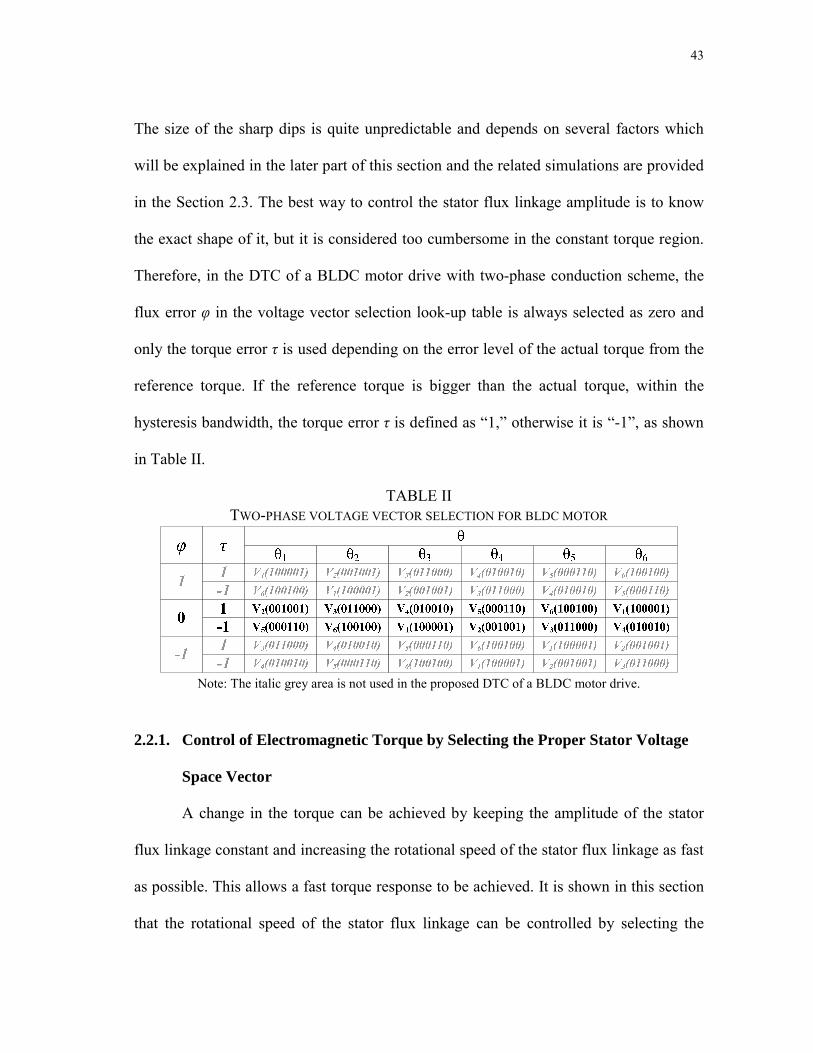
43
The size of the sharp dips is quite unpredictable and depends on several factors which
will be explained in the later part of this section and the related simulations are provided
in the Section 2.3. The best way to control the stator flux linkage amplitude is to know
the exact shape of it, but it is considered too cumbersome in the constant torque region.
Therefore, in the DTC of a BLDC motor drive with two-phase conduction scheme, the
flux error φ in the voltage vector selection look-up table is always selected as zero and
only the torque error τ is used depending on the error level of the actual torque from the
reference torque. If the reference torque is bigger than the actual torque, within the
hysteresis bandwidth, the torque error τ is defined as “1,” otherwise it is “-1”, as shown
in Table II.
TABLE II TWO-PHASE VOLTAGE VECTOR SELECTION FOR BLDC MOTOR
Note: The italic grey area is not used in the proposed DTC of a BLDC motor drive.
2.2.1. Control of Electromagnetic Torque by Selecting the Proper Stator Voltage
Space Vector
A change in the torque can be achieved by keeping the amplitude of the stator
flux linkage constant and increasing the rotational speed of the stator flux linkage as fast
as possible. This allows a fast torque response to be achieved. It is shown in this section
that the rotational speed of the stator flux linkage can be controlled by selecting the

44
proper voltage vectors while keeping the flux amplitude almost constant, in other words
eliminating the flux control.
1SW
dcV
3SW 5SWsR
sL M−
aece
be
sR
sR
1SW 2SW 3SW 4SW 5SW 6SW
4SW2SW 6SW
C
CsL M−
sL M−
Fig. 2.2. Representation of two-phase switching states of the inverter voltage space vectors for a
BLDC motor.
When the primary windings, which are assumed to be symmetric fed by an
inverter using two-phase conduction mode, as shown in Fig. 2.2, the primary voltages,
Van, Vbn, and Vcn, are determined by the status of the six switches: SW1, SW2, …., and
SW6. For example, if SW1 is one (turned on), SW2 is zero (turned off), SW3 is zero, and
SW4 is one then Van = Vdc/2 and Vbn = −Vdc/2 (phase–c is open meaning that SW5 and
SW6 are zero). Since the upper and lower switches in a phase leg may both be
simultaneously off, irrespective of the state of the associated freewheeling diodes in two-
phase conduction mode, six digits are required for the inverter operation, one digit for
each switch [56]. Therefore, there is a total of six non-zero voltage vectors and a zero
voltage vector for the two-phase conduction mode which can be represented as V0,1,2,…,6
(SW1, SW2, …., SW6), as shown in Fig. 2.1. The six non-zero vectors are 60 degrees

45
electrically apart from each other, as depicted in Fig. 2.1, but 30 electrical degrees phase
shifted from the corresponding three-phase voltage vectors which are used in three-phase
conduction DTC of a PMSM drive. Stationary reference frame (αβ–axes) representations
of the six non-zero voltage vectors with respect to dc-link voltage and switching states of
the semiconductor devices are derived in Appendix C. The overall block diagram of the
closed-loop DTC scheme of a BLDC motor drive in the constant torque region is
represented in Fig. 2.3. The dotted area represents the stator flux linkage control part of
the scheme used only for comparison purposes. When the two switches in Fig. 2.3 are
changed from state 2 to state 1, flux control is considered in the overall system along
with torque control. In the two-phase conduction mode the shape of stator flux linkage
trajectory is ideally expected to be hexagonal, as illustrated with the straight dotted line
in Fig. 2.1. However, the influence of the unexcited open-phase back-EMF causes each
straight side of the ideal hexagonal shape of the stator flux linkage locus to be curved
and the actual stator flux linkage trajectory tends to be more circular in shape, as shown
in Fig. 2.1 with solid curved line [56]. In addition to the sharp changes, curved shape in
the flux locus between two consecutive commutations complicates the control of the
stator flux linkage amplitude because it depends on the size of the sharp dips, and the
depth of the change may vary with sampling time, dc-link voltage, hysteresis bandwidth,
motor parameters especially the phase inductance, motor speed, snubber circuit, and the
amount of load torque. For example, if the phase inductance is low the current and
torque ripples in the direct torque controlled motor drives will be much higher compared
to the machines with higher phase inductance. Therefore, to obtain low current and

46
30
()
3(
)(
)2
2em
es
es
PT
ki
ki
αα
ββ
θθ
=+
()
() dt
iR
V
dti
RV
ss
ss
sas
ss
∫∫−
=
−=
ββ
β
αα
ϕϕ2
2β
αϕ
ϕϕ
ss
s+
=
⎟⎟ ⎠⎞⎜⎜ ⎝⎛
−
αβ
ϕϕ ss1
tansθ
()
se
ϕθ
∗
eθmθ
2P
∗emT
Fig.
2.3
. Ove
rall
bloc
k di
agra
m o
f the
two-
phas
e co
nduc
tion
DTC
of a
BLD
C m
otor
driv
e in
the
cons
tant
torq
ue re
gion
.

47
torque ripples in direct torque controlled motor drives, machines with high inductance
are preferred.
If a BLDC motor has an ideal trapezoidal back-EMF having a 120 electrical
degree flat top, one current sensor on the dc-link can be used to estimate the torque. By
knowing the sectors using hall-effect sensors the torque can be estimated with Tem =
2keidc, where ke is the back-EMF constant and idc is the dc-link current. In reality, this
might generate some low-frequency torque oscillations due to the approximation of the
back-EMF as ideal trapezoid. To achieve a more accurate torque estimation, in general,
for non-sinusoidal surface-mounted permanent magnet motors it is suggested that (2.16)
should be used.
Usually the overall control system of a BLDC motor drive includes three hall-
effect position sensors mounted on the stator 120 electrical degrees apart. These are used
to provide low ripple torque control if the back-EMF is ideally trapezoidal because
current commutation occurs only every 60 electrical degrees, as shown in Fig. 2.1.
Nevertheless, using high resolution position sensors is quite useful if the back-EMF of
BLDC motor is not ideally trapezoidal. The derivative of the rotor αβ–axes fluxes
obtained from (2.18) over electrical position will cause problems mainly due to the sharp
dips at every commutation point. The actual values of αβ–axes motor back-EMF
constants kα and kβ vs. electrical rotor position θe can be created in the look-up table,
respectively with great precision depending on the resolution of the position sensor (for
example incremental encoder with 2048 pulses/revolution), therefore a good torque
estimation can be obtained in (2.16). Figures representing the actual line-to-line and αβ–

48
axes back-EMF constants kab(θe), kbc(θe), kca(θe), kα(θe) and kβ(θe) are given in the
Appendix A, respectively.
2.3. Simulation Results
The drive system shown in Fig. 2.3 has been simulated for various cases with and
without stator flux control, switch states 1 and 2, respectively in order to demonstrate the
validity of the proposed two-phase conduction DTC of a BLDC motor drive scheme.
To set the gating signals of the power switches easily and represent the real
conditions in simulation as close as possible the electrical model of the actual BLDC
motor with R-L elements and the inverter with power semiconductor switches
considering the snubber circuit are designed in Matlab/Simulink® using the SimPower
Systems toolbox.
The dead-time of the inverter and non ideal effects of the BLDC machine are
neglected in the simulation model. The sampling interval is 25 μs. The switching table,
which is given in Table II is employed for the proposed DTC of the BLDC motor drive.
The magnitudes of the torque and flux hysteresis bands are 0.001 N·m, and 0.001 Wb,
respectively. It may be noted that the zero voltage vector suggested in [56] is not used in
the proposed scheme due to the reasons explained in Section 2.1.

49
-0.1 -0.05 0 0.05 0.1 0.15
-0.1
-0.05
0
0.05
0.1
0.15
Alfa-axis stator flux linkage (Wb)
Beta
-axi
s st
ator
flux
link
age
(Wb)
Fig. 2.4. Simulated open-loop stator flux linkage trajectory under the two-phase conduction DTC
of a BLDC motor drive at no load torque (speed + torque control).
Figs. 2.4 and 2.5 show the simulation results of the uncontrolled open-loop stator
flux linkage locus when 0 N·m and 1.2835 N·m load torque are applied to the BLDC
motor with ideal trapezoidal back-EMF, respectively. Fig. 2.4 represents the removal of
the free-wheeling diode effect on flux locus with unloaded condition. Steady-state speed
control is performed with an inner-loop torque control without flux control. Stator flux
linkage is estimated using (2.18) as an open-loop. As can be seen in Fig. 2.5 when the
load torque level increases, more deep sharp changes are observed which increases the
difficulty of the flux control if it is used in the control scheme. The steady-state speed is
30 mechanical rad/s and the dc-link voltage Vdc equals 40 2 V. Since the speed is
controlled a better open-loop circular flux trajectory is obtained.

50
Under only torque control, when the zero voltage vector V0 is used to decrease
the torque, as suggested in [56], larger, more frequent spikes on the phase voltages are
observed in Fig. 2.6 compared to the ones used from the suggested voltage vector look-
up table given in Table II.
-0.1 -0.05 0 0.05 0.1 0.15
-0.1
-0.05
0
0.05
0.1
0.15
Alfa-axis stator flux linkage (Wb)
Beta
-axi
s st
ator
flux
link
age
(Wb)
Fig. 2.5. Simulated open-loop stator flux linkage trajectory under the two-phase conduction DTC
of a BLDC motor drive at 1.2835 N·m load torque (speed + torque control).
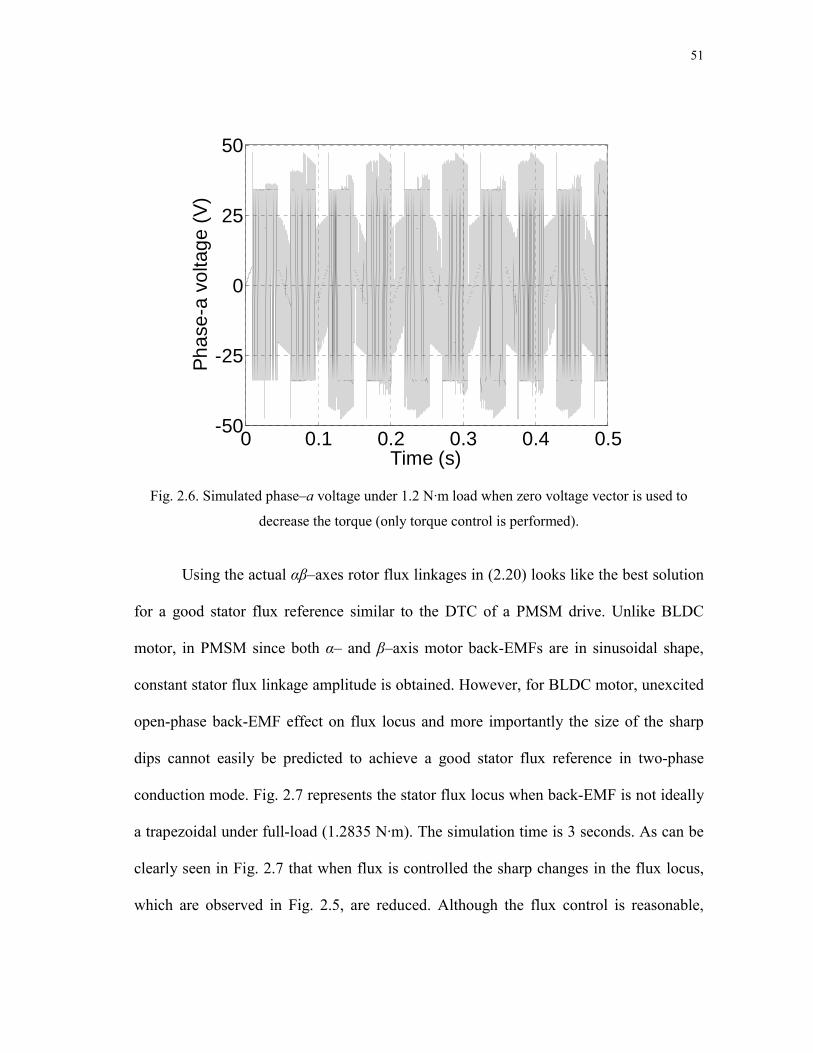
51
0 0.1 0.2 0.3 0.4 0.5-50
-25
0
25
50
Time (s)
Phas
e-a
volta
ge (V
)
Fig. 2.6. Simulated phase–a voltage under 1.2 N·m load when zero voltage vector is used to
decrease the torque (only torque control is performed).
Using the actual αβ–axes rotor flux linkages in (2.20) looks like the best solution
for a good stator flux reference similar to the DTC of a PMSM drive. Unlike BLDC
motor, in PMSM since both α– and β–axis motor back-EMFs are in sinusoidal shape,
constant stator flux linkage amplitude is obtained. However, for BLDC motor, unexcited
open-phase back-EMF effect on flux locus and more importantly the size of the sharp
dips cannot easily be predicted to achieve a good stator flux reference in two-phase
conduction mode. Fig. 2.7 represents the stator flux locus when back-EMF is not ideally
a trapezoidal under full-load (1.2835 N·m). The simulation time is 3 seconds. As can be
clearly seen in Fig. 2.7 that when flux is controlled the sharp changes in the flux locus,
which are observed in Fig. 2.5, are reduced. Although the flux control is reasonable,

52
unwanted current amplitude is generated as seen in Fig. 2.8 to keep the torque and flux
in the desired level.
-0.1 -0.05 0 0.05 0.1 0.15
-0.1
-0.05
0
0.05
0.1
0.15
Alfa-axis stator flux linkage (Wb)
Beta
-axi
s st
ator
flux
link
age
(Wb)
Fig. 2.7. Simulated stator flux linkage locus with non-ideal trapezoidal back-EMF under full load
(speed + torque + flux control).
Even though the torque control still exists for some time with low-frequency
oscillations, motor will be damaged because of high terminal current exceeding the peak
current of 24 A, as shown in Fig. 2.8. Instability in the torque compared to the current
does not occur except high ripples because hysteresis torque and flux controllers try to
correct the errors in the torque and flux by applying unwanted voltage vectors. There is
higher voltage than what is expected (~ 34 V) in the motor terminals compared to when
just torque control is used without flux control. Because large and distorted terminal
voltages exist, higher and distorted phase currents as seen in Fig. 2.8 are obvious. All

53
these problems are because of the flux control. There should be exact flux amplitude to
be given as a reference flux value including sharp changes at every commutation points
and curved shape between those commutation points, then appropriate flux control can
be obtained without losing the torque control. However, to predict all these
circumstances to generate a flux reference is cumbersome work which is unnecessary in
the constant torque region.
0 1 2 3-30
-20
-10
0
10
20
30
40
Time (s)
Phas
e-a
curr
ent (
A)
Fig. 2.8. Simulated phase–a current when flux control is obtained using (2.20) under full load
(speed + torque + flux control).

54
0.15 0.2 0.25 0.3 0.35 0.4-6
-4
-2
0
2
4
6
Time (s)
Phas
e-a
curr
ent (
A)
Fig. 2.9. Simulated phase–a current when just torque is controlled without flux control under 1.2
N·m load with non-ideal trapezoidal back-EMF (reference torque is 1.225 N·m).
0 0.1 0.2 0.3 0.4 0.50
0.2
0.4
0.6
0.8
1
1.2
1.4
Time (s)
Elec
trom
agne
tic to
rque
(N.m
)
Fig. 2.10. Simulated electromagnetic torque when just torque is controlled without flux control
under 1.2 N·m load with non-ideal trapezoidal back-EMF (reference torque is 1.225 N·m).

55
0.15 0.2 0.25 0.3 0.35 0.4-50
-25
0
25
50
Time (s)
Phas
e-a
volta
ge (V
)
Fig. 2.11. Simulated phase–a voltage when just torque is controlled without flux control under
1.2 N·m load with non-ideal trapezoidal back-EMF (reference torque is 1.225 N·m).
Figs. 2.9–2.11 show phase–a current, electromagnetic torque and phase–a
voltage, respectively under only torque control when the back-EMF is not ideally
trapezoidal considering only the first, third and fifth harmonics of the fundamental ideal
trapezoidal back-EMF. Reference torque is 1.225 N·m and the load torque is 1.2 N·m,
thereby speed is kept at around 55 electrical rad/s for a better circular flux locus. If high
resolution position sensor such as incremental encoder is used instead of the three hall-
effect sensors, low-frequency torque oscillations can be minimized by using (2.16), as
shown in Fig. 2.10. In (2.16), the product of the actual αβ–axes back-EMF constants by
the corresponding αβ–axes currents and number of pole pairs provide the exact values of
the α– and β–axis torque, respectively.

56
2.4. Experimental Results
The feasibility and practical features of the proposed DTC scheme of a BLDC
motor drive have been evaluated using an experimental test-bed, as shown in Fig. 2.12.
The proposed control algorithm is digitally implemented using the eZdspTM board from
Spectrum Digital, Inc. based on TMS320F2812 DSP, as shown in Fig 2.12(a). In Fig.
2.12(b), the BLDC motor whose parameters are given in the Appendix A is coupled to
the overall system.
In this section, transient and steady-state torque and current responses of the
proposed two-phase conduction DTC scheme of a BLDC motor drive are demonstrated
experimentally under 0.2 pu load torque condition. The experimental results are obtained
from the datalog (data logging) module in the Texas Instruments Code Composer
StudioTM IDE software.
Fig. 2.13(a) and (b) illustrate the experimental results of the phase–a current and
torque, respectively when only torque control is performed using (2.16), as shown in Fig.
2.3 with switch state 1. In Fig. 2.13(b), the reference torque is suddenly increased from
0.225 pu to 0.45 pu at 9.4 ms under 0.2 pu load torque. One per-unit is 1.146 N·m for
torque, 5 A for current, and 1800 rpm for speed. The sampling time is chosen as 1/30000
second, hysteresis bandwidth is 0.001 N·m, dead-time compensation is included, and the
dc-link voltage is set to Vdc = 40 2 V. As it can be seen in Fig. 2.13(a) and (b), when
the torque is suddenly increased the current amplitude also increases and fast torque
response is achieved. The high frequency ripples observed in the torque and current are
related to the sampling time, hysteresis bandwidth, winding inductance, and dc-link

57
voltage. This is well in accordance with the simulation results in Figs. 2.9 and 2.10
where the sampling time is chosen as 25 μs.
(a)
(b)
Fig. 2.12. Experimental test-bed. (a) Inverter and DSP control unit. (b) BLDC motor coupled to
dynamometer and position encoder (2048 pulse/rev).
BLDC Motor
Hysteresis Brake
Position Encoder
SEMIKRON Inverter
eZdsp2812

58
Pha
se-a
cur
rent
[1.2
5 A/
div]
Time [3.4 ms/div]
0
(a)
Ele
ctro
mag
netic
torq
ue [0
.285
6 N
.m/d
iv]
Time [3.4 ms/div]
0
(b)
Fig. 2.13. (a) Experimental phase–a current and (b) electromagnetic torque under 0.2292 N·m
(0.2 pu) load.

59
2.5. Conclusion
This study has successfully demonstrated application of the proposed two-phase
conduction direct torque control (DTC) scheme for BLDC motor drives in the constant
torque region. A look-up table for the two-phase voltage vector selection is designed to
provide faster torque response both on rising and falling conditions. Compared to the
three phase DTC technique, this approach eliminates the flux control and only torque is
considered in the overall control system. Three reasons are given for eliminating the flux
control. First, since the line-to-line back-EMF including the small voltage drops is less
than the dc-link voltage in the constant torque region there is no need to control the flux
amplitude. Second, with the two-phase conduction mode sudden sharp dips in the stator
flux linkage locus occur that complicate the control scheme. The size of these sharp dips
is unpredictable. Third, regardless of the stator flux linkage amplitude, the phase currents
tend to match with the flat top portion of the corresponding trapezoidal back-EMF to
generate constant torque.

60
CHAPTER III
POWER FACTOR CORRECTION OF DIRECT TORQUE CONTROLLED
BRUSHLESS DC MOTOR WITH NON-SINUSOIDAL BACK-EMF USING
TWO-PHASE CONDUCTION MODE
3.1. Introduction
In general, ac motor drives have very poor power factor due to the high number
of harmonics in the line current. Power factor correction (PFC) method is a good
candidate for ac-dc switched mode power supply in order to reduce the harmonics in the
line current, increase the efficiency and capacity of motor drives, and reduce customers’
utility bills. There are two general types of PFC methods to obtain a unity power factor:
analog and digital PFC techniques. In the past, due to the absence of fast
microprocessors and DSPs, analog PFC methods were the only choice for achieving the
unity power factor. Many control strategies using analog circuits have been explored in
the past, including average current control [59], peak current control [60], hysteresis
control [61], nonlinear carrier control [62], etc. With the recent developments in the
microprocessor and DSP technologies, there is a possibility of implementing the
complicated PFC algorithms using these fast processors [63].
As compared to conventional analog controllers, digital regulators offer several
advantages such as possibility of implementing nonlinear and sophisticated control

61
algorithms, reduction of the number of control components, high reliability, low
sensitivity to component aging, better performance than that in analog implementation
with the same cost, reduced susceptibility to environmental variations such as thermal
drifts, and negligible offsets.
Digital control PFC implementations have been investigated by many researchers
[64]–[66]. Majority of the work has been done on the implementation of the analog PFC
techniques in the digital platform. There has been very little work done in the literature
to implement the digital PFC methods on ac motor drives. The basic idea of the
proposed PFC method in this paper is to update the required amount of duty cycle for
boost converter in every sampling time of the DTC of BLDC motor drive.
In this section, first of all the principle of the average current control boost PFC
with feed-forward voltage compensation technique is presented in Section 3.2. In
Section 3.3, the hardware implementation and experimental results of the proposed DTC
of BLDC motor drive in two-phase conduction mode using average current control with
input voltage feed-forward compensation boost PFC including load disturbance are
presented. The conclusion is presented in Section 3.4.

62
mθ
eθ2P
1(
2)
3
ssa
ssa
sb
ii
ii
i
α β
= =+
3 22
ems
se
eee
PΤ
ii
βα
αβ
ωω
⎛⎞ ⎟
⎜⎟
=+
⎜⎟
⎜⎟
⎜ ⎝⎠
eθ
Fig.
3.1
. Ove
rall
bloc
k di
agra
m o
f the
two-
phas
e co
nduc
tion
DTC
of a
BLD
C m
otor
driv
e w
ith b
oost
PFC
in th
e co
nsta
nt to
rque
regi
on.

63
3.2. The Average Current Control Boost PFC With Feed-Forward Voltage
Compensation
The main topology of the power factor pre-regulator based on boost converter
includes two parts: rectifier circuit and boost circuit. The block diagram and DSP control
stage of the boost PFC using average current control with feed-forward voltage
compensation is shown in Fig. 3.1. As can be seen in Fig. 3.1, in contrast to the
conventional boost circuit, the large filter capacitor of the power factor pre-regulator is
placed at the output of the system. As indicated in Fig. 3.1, three signals are required to
implement the control algorithm. These are, the rectified input voltage Vin, the inductor
current Iin, and the dc output voltage Vo. There are two feedback loops in the control
system. The average output dc voltage Vo is regulated by a slow response (high
bandwidth), whereas the inner loop that regulates the input current Iin is a much faster
loop (low bandwidth).
For the purpose of digital control of a boost PFC converter, the instantaneous
analog signals Vin, Iin, and Vo are all sensed and fed back to the DSP via three ADC
channels ADCIN2, ADCIN3, and ADCIN4 at every sampling period, Ts respectively.
Then they are converted to the per-unit equivalents using the gain blocks. The per-unit
output voltage Vo(pu) is compared to the desired per-unit reference voltage Vref(pu) and the
difference signal (Vref(pu) − Vo(pu)) is then fed into the voltage loop controller Gv. The
output of the Gv, indicated as B, controls the amplitude of the per-unit reference current
Iref(pu) such that for the applied load current and line voltage, the output voltage Vo is
maintained at the reference level. Then, it is multiplied by the two other feed-forward
64
components, A and C, to generate the reference current command for the inner current
loop. In Fig. 3.1, the component A represents the digitized instantaneous per-unit input
sensed signal Vin and the component C is one over square of the per-unit averaged input
voltage which equals 1/Vdc(pu)2. The derivation of the feed-forward voltage component C
is given in Section 3.2.1. The per-unit reference current command Iref(pu) for the inner
current loop has the shape of a rectified sinewave and its amplitude is such that it
maintains the per-unit output dc voltage Vo(pu) at per-unit reference voltage Vref(pu) level
overcoming load and input voltage disturbances. The difference signal (Iref(pu) − Iin(pu)) is
then passed into the current loop controller Gi in which the PWM duty ratio command is
generated for the boost converter switch to maintain the per-unit inductor current Iin(pu) at
the per-unit reference current Iref(pu) level. The multiplier gain Km whose derivation is
provided in Section 3.2.1 is also added to the control block which allows adjustments of
the per-unit reference current Iref(pu) signal based on the converter input voltage operating
range Vmin – Vmax [67].
3.2.1. Calculation of Feed-Forward Voltage Component C and Multiplier Gain Km
For simplicity per-unit system has been used to describe the components and all
variables in the control system. Therefore, the voltage and current signals are
automatically saved as per-unit (pu) numbers normalized with respect to their own
maximum values.
The multiplier gain Km is useful to adjust the reference current at its maximum
when the PFC boost converter delivers the maximum load at the minimum input voltage

65
Vin. In Fig. 3.1, per-unit reference current Iref(pu) is expressed in terms of Km, A, B, and C
as follows:
( )ref pu mI K ABC= (3.1)
where A is the per-unit value of the sensed input voltage Vin, B is the output of the
voltage PI controller Gv, and C is the inverse square of the averaged input rectified
voltage Vdc, respectively.
The average per-unit value Vdc(pu) of the input per-unit voltage Vin(pu) is given as
( ) ( )
0
1 T
dc pu in puV V dtT
= ∫ (3.2)
where T is the time period of the input voltage corresponding to the grid frequency
which is 60 Hz in this case and Vin(pu) is the per-unit value of the input rectified voltage
normalized with respect to its maximum peak value Vmax. In (3.2), the base value of the
per-unit average rectified input voltage Vdc(pu) is also chosen as Vmax.
The maximum value of the average value Vdc of the sinewave input voltage is
only 2Vmax/π. Therefore, the final per-unit representation of the average per-unit voltage
Vdc(pu) is given by
( )( ) ( ) (2 / ) 2
dc pumaxdcx pu dc pu
max
VVV VV
ππ
= = (3.3)
The inverse per-unit voltage Vinv(pu) of the average per-unit component Vdc(pu) of
the per-unit input voltage Vin(pu) can be calculated as follows:
For per-unit representation of the average inverse voltage Vinv, maximum inverse
voltage Vinv_max should be found which equals the inverse minimum of the average input

66
voltage 1/Vdc_min = π/(2Vmin) where Vmin is the minimum peak amplitude of the rectified
input voltage selected based on the input operating voltage range of the PFC boost
converter. Finally, the per-unit value of the inverse voltage Vinv(pu) in terms of Vdc(pu),
Vmin, and Vmax is given as
( )( )
12dcx pu dc _ max min
inv puinv _ max dc( pu ) max
V V VVV V Vπ
⎛ ⎞⎜ ⎟⎜ ⎟⎝ ⎠= = (3.4)
where Vdc_max is the maximum average input rectified voltage equals 1/Vinv_min = 2Vmax/π.
In (3.4), the numerator in parentheses represents the non per-unit value of the inverse
average input voltage Vinv.
Once the inverse per-unit voltage Vinv(pu) is calculated, the feed-forward voltage
component C can be found as
22 min
( ) 2 2( ) max ( )
4 4( ) ( )inv pu
dc pu dc pu m
VC VV V V Kπ π
⎛ ⎞= = =⎜ ⎟
⎝ ⎠ (3.5)
where the multiplier gain Km can be expressed using (3.1) such that the reference per-
unit current Iref(pu) is at its maximum when the PFC boost converter delivers the
maximum load at the minimum operating input voltage as
max
minm
VKV
= (3.6)
The overall block diagram of the closed-loop DTC scheme of a BLDC motor
drive with average current control boost PFC in the constant torque region is represented
in Fig. 3.1. In Fig. 3.1, since there is no PWM generation required in the proposed DTC
67
scheme, six GPIO pins for DTC scheme and only one PWM output pin for PFC
algorithm are used to achieve the overall closed-loop control.
3.3. Experimental Results
The feasibility and practical features of the proposed DTC scheme of a BLDC
motor drive with average current control boost PFC have been evaluated using an
experimental test-bed, shown in Fig. 3.2. The proposed control algorithm is digitally
implemented using the eZdspTM board from Spectrum Digital, Inc. based on a fixed-
point TMS320F2812 DSP, as shown in Fig 3.2(a). In Fig. 3.2(b), the BLDC motor
whose parameters are given in the Appendix A is coupled to the overall system.
The average current control boost PFC with feed-forward voltage compensation
method has been implemented in a single sampling time of the proposed DTC of a
BLDC motor drive under two-phase conduction mode in the constant torque region. The
boost converter switch is FET47N60C3, and the diode is STTH8R06D. The passive
components of the boost converter are the inductor L3 = 1 mH and output filter
capacitors C3 = C4 = 270 μF, as seen in Fig. 3.1. The boost converter switches at 80 kHz
which is the sampling frequency of the overall control system and supplies 80 Vdc at the
output. The input voltage range, Vmin – Vmax, is 28.28 Vac – 70.71 Vac peak. The EMI
filter is used in order to reduce the high order switching harmonics in the line current
which consists of the inductors L1 = L2 = 10 μH and the capacitors C1 = C2 = 1 μF.
Gain of the feed forward path Km = 2.5 was selected in this implementation. In
this paper, digital proportional-integral (PI) controllers are used in the voltage and

68
current loops. The coefficients of the PI voltage and current controllers are chosen as Kpv
= 0.1736, Kiv = 0.01388, Kpi = 0.005, and Kii = 0.03125, respectively. One per-unit is
1.146 N·m for torque, 5 A for current, and 1800 rpm for speed. Hysteresis bandwidth is
0.001 N·m, and the dead-time compensation is included as well.
In the implementation, over-current and voltage protections have been used for
the inductor current and output voltage. Once the sensed inductor current and output dc
voltage are higher than 8 A and 140 V, respectively a protection logic signal is generated
and used to turn off the gate signal of the boost converter.
Steady-state current response of the proposed two-phase conduction DTC
scheme of a BLDC motor drive with average current control boost PFC is demonstrated
experimentally under 0.371 N·m load torque condition in Fig. 3.3 where the reference
torque is 0.573 N·m. The experimental results are obtained from the datalog (data
logging) module in the Texas Instruments Code Composer StudioTM IDE software. The
high frequency ripples in the current observed in Fig. 3.3 depend on the hysteresis
bandwidth of the torque control, sampling time, especially motor winding inductance,
and the amount of dc-link voltage. Because the machine used in the tests has low
winding inductance and the dc-link is selected quite high for better power factor, the
current ripples are expected to be high as seen in Fig. 3.3.

69
(a)
(b)
Fig. 3.2. Experimental test-bed. (a) Inverter, DSP control unit, and boost PFC board. (b) BLDC
motor coupled to dynamometer and position encoder (2048 pulse/rev.).
Fig. 3.4 shows the measured output voltage, line voltage, and line current
waveforms for the two-phase DTC of BLDC motor drive at no load and at the steady-
state without PFC. The power factor under this operating condition is 0.7667. The
SEMIKRON Inverter
eZdsp2812 Boost PFC
BLDC Motor
Hysteresis Brake
Position Encoder

70
measured total harmonic distortion of the input line current and line voltage are 82.23%
and 4.79%, respectively. The output active power is 55.3 W.
Fig. 3.3. Measured steady-state phase-a current of two-phase DTC of BLDC motor drive using
boost PFC under 0.371 N·m load with 0.573 N·m reference torque. Current: 1.25 A/div. Time
base: 0.7 ms/div.

71
Fig. 3.4. Measured output dc voltage Vo, line voltage Vline, and line current Iline without PFC
under no load with 0.4 N·m reference torque. (Top) Output dc voltage Vo = 80 V. (Middle) Line
voltage Vline = 64.53 Vrms. (Bottom) Line current Iline = 1.122 A. Vo: 20 V/div; Iline: 2 A/div; Vline:
50 V/div. Time base: 5 ms/div.
Since no PFC control has been applied to the two-phase conduction DTC of
BLDC motor drive, the power factor is poor and the line current has harmonics in it as
can be seen in Fig. 3.4. Moreover, the output dc voltage also has some fluctuations due
to the absence of the PFC control. These problems can be eliminated by using a PFC
control algorithm during a single sampling period of the DTC of BLDC motor drive
system.
The output dc voltage, input line current, and line voltage waveforms for the two-
phase DTC of BLDC motor control at no load and at the steady-state with average

72
current control boost PFC are shown in Fig. 3.5. The measured total harmonic distortion
of the input line current and line voltage are 5.45% and 3.45%, respectively and the
measured power factor is 0.9997. The output active power of the total system is 69.3 W.
Since the PFC algorithm is adapted to the overall DTC of BLDC motor drive system,
low-frequency oscillations on dc-link voltage is reduced and the line current is more
sinusoidal, thereby eliminating harmonics as seen in Fig. 3.5 compared to the ones
shown in Fig. 3.4. Thus, the power factor and the efficiency of the total system are
improved considerably.
Fig. 3.5. Measured steady-state output dc voltage Vo, line voltage Vline, and line current Iline with
PFC under no load with 0.4 N·m reference torque. (Top) Output dc voltage Vo = 80 V. (Middle)
Line voltage Vline = 25.43 Vrms. (Bottom) Line current Iline = 2.725 A. Vo: 20 V/div; Iline: 5 A/div;
Vline: 50 V/div. Time base: 5 ms/div.

73
Fig. 3.6 shows the measured output voltage, line voltage, and line current
waveforms for the two-phase DTC of BLDC motor control under 0.371 N·m load at the
steady-state with PFC. The power factor under this operating condition is 0.9997. The
measured total harmonic distortion of the input line current and line voltage are 5.05%
and 3.43%, respectively. The output active power of the total system in this case is 108.6
W.
Due to the existence of the load torque, output dc voltage in Fig. 3.6 has some
distortion as compared to the dc output voltage shown in Fig. 3.5. There has not been a
significant difference observed in the line currents and line voltages between Fig. 3.5
and Fig. 3.6.
Fig. 3.6. Measured steady-state output dc voltage Vo, line voltage Vline, and line current Iline with
PFC under 0.371 N·m load with 0.573 N·m reference torque. (Top) Output dc voltage Vo = 80 V.
(Middle) Line voltage Vline = 25.2 Vrms. (Bottom) Line current Iline = 4.311 A. Vo: 20 V/div; Iline: 5
A/div; Vline: 50 V/div. Time base: 5 ms/div.

74
3.4. Conclusion
The digital implementation of the DTC for BLDC motor drive using two-phase
conduction mode with average current control boost PFC during a single sampling
period of the motor drive system has been successfully demonstrated on an eZdspTM
board featuring a TMS320F2812 DSP. A prototype boost PFC controlled by a DSP
evaluation board was built to verify the proposed digital control PFC strategy along with
the DTC of BLDC motor drive system. Experimental results show that, based on the
proposed average current control boost PFC with input voltage compensation algorithm,
the power factor of 0.9997 is achieved at the steady-state under 20 to 50 Vrms input
voltage range conditions. Moreover, the proposed PFC control strategy can achieve
smooth output dc voltage which is applied to the BLDC motor drive and sinusoidal line
current waveform with THD as low as 5%. Therefore, the power factor and the overall
efficiency of the DTC of BLDC motor drive are increased considerably.

75
CHAPTER IV
DIRECT TORQUE CONTROL OF FOUR-SWITCH BRUSHLESS DC MOTOR
WITH NON-SINUSOIDAL BACK-EMF USING TWO-PHASE CONDUCTION
MODE
4.1. Introduction
Brushless dc motors have been used in variable speed drives for many years due
to their high efficiency, high power factor, high torque, simple control, and lower
maintenance [41]. Low cost and high efficiency variable speed motor drives have had
growing interest over the years. Minimizing the switch counts has been proposed to
replace the traditional six-switch three-phase inverter. Van Der Broeck has demonstrated
the possibility to implement a three phase ac motor drive system employing the four-
switch three phase inverter [68]. In [68], although the topology of the four-switch
inverter for the induction motor is identical to the BLDC motor, conventional four-
switch PWM schemes used for induction motor drives cannot be directly applied to
BLDC motor drive. Three phase conduction scheme is presented which is inherently
difficult to use in brushless dc motor drive systems incorporating only 120 electrical
degree current conduction. This is due to the limited voltage space vectors of the
conventional four-switch scheme. Therefore, in order to use the four-switch inverter
topology for the three-phase BLDC motor drive, only two phase conduction voltage
space vectors (line-to-line voltage vectors) should be obtained from the four-switch

76
inverter. This theory is presented in [69] where special current control method is
performed for the two modes of operation (mode 2 and 5) such that when two phases
which are not connected to the center of the dc-link capacitors conduct, they are
individually controlled by the hysteresis PWM current controllers. By doing so, current
distortions on each phase caused by the back-EMF of the inactive third phase, which is
connected to the center part of the split dc-link capacitors, are reduced.
One of the other solutions to the limited voltage space vector problem is to
modify the conventional voltage controlled PWM strategies, such as space vector PWM
technique presented in [70, 71]. However, in [70, 71] several proportional and integral
controllers are needed along with abc to αβ (stationary reference frame) and αβ to abc
transformations for both currents and voltages. Moreover, reference current generation
scheme is proposed which requires commutation interval times. Those interval times are
dependant on several motor parameters such as winding inductance, dc-link voltage and
back-EMF. Therefore, more complicated and parameter sensitive drive system is
inevitable.
The most popular way to control BLDC motors using four- or six-switch inverter
is by PWM current control in which a two-phase feeding scheme is considered with
variety of PWM modes such as soft switching, hard-switching, and etc. In this work,
unlike the methods discussed in [68, 70, 71], a novel direct torque control scheme
including the actual pre-stored back-EMF constants vs. electrical rotor position look-up
table is proposed for BLDC motor drive with two-phase conduction scheme using four-
switch inverter. Therefore, low-frequency torque ripples and torque response time are

77
minimized compared to conventional four-switch PWM current and voltage controlled
BLDC motor drives. This is achieved by properly selecting the inverter voltage space
vectors of the two-phase conduction mode from a simple look-up table at a predefined
sampling time.
It is believed that the direct torque controlled BLDC motor drive compared to a
PWM voltage controlled one has higher dynamic speed/torque response and does not
rely on some tedious calculations. Instead, the DTC of a BLDC motor drive depends on
a keen and detailed observation of the overall operation, so that it dramatically reduces
equations from the conventional control scheme, such as space vector PWM and etc. and
is simple to implement from the hardware and software points of view [69].
The four-switch DTC of a BLDC motor drive operating in two-phase conduction
mode which is similar to [72] is simplified to just a torque controlled drive by
intentionally keeping the stator flux linkage amplitude almost constant by eliminating
the flux control in the constant torque region. It is shown that in the constant torque
region under the two-phase conduction DTC scheme using four-switch (or six-switch)
inverter, the amplitude of the stator flux linkage cannot easily be controlled due to the
sharp changes and the curved shape of the flux vector between two consecutive
commutation points in the stator flux linkage locus. Since the flux control along with
PWM generation is removed, fewer algorithms are required for the proposed control
scheme.
Specifically, it is shown that rather than attempting to control the stator flux
amplitude in two-phase conduction DTC of BLDC motor drive, only the electromagnetic

78
torque is controlled. It will be shown that due to the sharp changes, which occur every
60 electrical degrees, flux amplitude control is quite difficult. Moreover, it will be
explained in detail that there is no need to control the stator flux linkage amplitude of a
BLDC motor in the constant torque region. The stator flux linkage position in the
trajectory is helpful to find the right sector for the torque control in sensorless
applications of BLDC motor drives. Therefore, the torque is controlled while the stator
flux linkage amplitude is kept almost constant on purpose [72]. In the proposed method,
a simple two-phase four-switch inverter voltage space vector look-up table is developed
to control the electromagnetic torque. Moreover, to obtain smooth torque characteristics
a new switching logic is designed and incorporated with the two-phase four-switch
voltage space vector look-up table. Simulated and experimental results are presented to
illustrate the validity and effectiveness of the two-phase four-switch DTC of a BLDC
motor drive in the constant torque region.
4.2. Topology of the Conventional Four-Switch Three-Phase AC Motor Drive
4.2.1. Principles of the Conventional Four-Switch Inverter Scheme
In four-switch three-phase inverter system, there are four possible switching
patterns to generate three-phase currents, as shown in Fig. 4.1 with ideal switches; these
four switching patterns are (0, 0), (0, 1), (1, 0), and (1, 1) where “0” means the lower
switch is turned on and “1” the upper switch is turned on in each leg of the inverter. In
the same figure, the free-wheeling diodes as well as phase back-EMFs are ignored. As it
can be seen in Fig. 4.1 that in three-phase four-switch system the two switches on the
same leg never turn on and off at the same time. However, in six-switch inverter, two

79
zero voltage space vectors, (0, 0, 0) and (1, 1, 1), cannot supply the dc-link to the load,
therefore no current flows through the load. The main difference of the four-switch
inverter compared to its counterpart six-switch one is that one phase is always connected
to the center tap of the split capacitors, so that there will always be current flowing
through that phase even with voltage vectors (0, 0) and (1, 1), as shown in Fig. 4.1.
Under balanced load condition with four-switch topology, there will be no current flow
through the phase which is connected to the midpoint of the split capacitors using two
possible non-zero voltage vectors, (1, 0) and (0, 1), as seen in Fig. 4.1. When voltage
vectors (1, 0) and (0, 1) are used and the load is not completely balanced, only the
resultant current of the other two phases flow through the phase connected to the
midpoint of the split capacitors.
(a) (b)
(c) (d)
Fig. 4.1. Conventional four-switch voltage vector topology. (a) (0,0) vector, (b) (1,1) vector, (c)
(1,0) vector, and (d) (0,1) vector [69].

80
4.2.2. Applicability of the Conventional Method to the BLDC Motor Drive
Generating a 120 electrical degree current conduction is inherently difficult with
the conventional four-switch topology because a BLDC motor with non-sinusoidal back-
EMF (i.e. trapezoidal) requires a quasi-square wave current profile to generate constant
output torque compared to that of a permanent magnet synchronous motor with
sinusoidal back-EMF requiring sinewave current. These currents which have 120
electrical degrees conduction period are synchronized with the flat portion of the
corresponding phase back-EMFs, therefore a smooth electromagnetic torque can be
obtained. As a result, at every instant of time only two phases conduct and the other
phase is supposed to be inactive. Although four voltage vectors in conventional four-
switch inverter system are sufficient enough to control the three-phase ac motors using
PWM techniques, additional voltage vectors are required for BLDC motor with two-
phase conduction mode in order to control the midpoint current of the split capacitors at
a desired value. Since the conventional method cannot provide a two-phase conduction
method completely, a new control scheme with new switching patterns should be
developed such that only two of the three motor phases conduct. This will be explained
in detail in Section 4.3. Since for three phase ac induction motor and PMSM drives at
any instant of time there are always three-phase currents flowing through the machine,
summation of the three-phase currents under balanced condition is always zero. Also, at
any time none of the phase currents become zero. This scenario is not true for BLDC
motor with two-phase conduction where 120 electrical degrees of one complete cycle
(360 degree) of each phase currents will be zero. There will be cases where only phase–a

81
and –b currents are supposed to be conducting and phase–c current is zero as shown in
Mode II and V of Fig. 4.2. However, because of the phase back-EMF (phase–c) there
will be a current flowing in or out of phase–c through the dc-link. Therefore, special
attention should be given to the phase which is connected to the center of the split
capacitors in four-switch BLDC motor drive scheme.
Fig. 4.2. Actual (realistic) phase back-EMF, current, and phase torque profiles of the three-phase
BLDC motor drive with four-switch inverter.

82
4.3. The Proposed Four-Switch Direct Torque Control of BLDC Motor Drive
4.3.1. Principles of the Proposed Four-Switch Inverter Scheme
The key issue in the proposed four-switch DTC of a BLDC motor drive in the
constant torque region is to estimate the electromagnetic torque correctly similar to the
six-switch version given in [72]. For a surface-mounted BLDC motor the back-EMF
waveform is non-sinusoidal (trapezoidal), irrelevant of conducting mode (two or three-
phase), therefore (4.1) which is given in the stationary reference frame should be used
for the electromagnetic torque calculation [50, 56, 72].
3 3 ( ) ( )2 2 2 2em s e s es s
e e
eeP PT i i k i k iβαα α αβ β βθ θ
ω ω
⎡ ⎤⎡ ⎤⎢ ⎥= + = +⎢ ⎥⎣ ⎦⎢ ⎥⎣ ⎦
(4.1)
where P is the number of poles, θe is the electrical rotor angle, ωe is the electrical rotor
speed, and kα(θe), kβ(θe), eα, eβ, isα, isβ are the stationary reference frame (αβ–axes) back-
EMF constants, motor back-EMFs, and stator currents, respectively. Since the second
equation in (4.1) does not involve the rotor speed in the denominator there will be no
problem estimating the torque at zero and near zero speeds. Therefore, it is used in the
proposed control system instead of the one on the left in (4.1).
The αβ–axes rotor flux linkages φrα and φrβ are obtained as
r s s s
r s s s
L iL i
α α α
β β β
ϕ ϕϕ ϕ
= −= −
(4.2)
where φsα and φsβ are the α– and β–axis stator flux linkages, respectively. By using (4.2),
reference stator flux linkage command |φs(θe)|* for DTC of BLDC motor drive in the
constant torque region can be obtained similar to the DTC of a PMSM drive as

83
* 2 2( ) ( ) ( ) ( )s e r e r e r eα βϕ θ ϕ θ ϕ θ ϕ θ= = + (4.3)
Since the electromagnetic torque is proportional to the product of back-EMF and
its corresponding current, the phase currents are automatically shaped to obtain the
desired electromagnetic torque characteristics using (4.1). When the actual stationary
reference frame back-EMF constant waveforms from the pre-stored look-up table are
used in (4.1), much smoother electromagnetic torque is obtained as shown in Fig. 4.2.
From the detail investigation of the back-EMF, current, and phase torque profile
of the three-phase BLDC motor as shown in Fig. 4.2, one can obtain a solution to the
problems that occur in the conventional four-switch topology explained in Section 4.2.2.
As can be observed in Fig. 4.2 that to generate constant electromagnetic torque due to
the characteristics of the BLDC motor, such as two-phase conduction, only two of the
three phase torque are involved in the total torque equation during every 60 electrical
degrees and the remaining phase torque equals zero as shown in Table III. The total
electromagnetic torque of PMAC motors equals the summation of each phase torque
which is given by
em ea eb ecT T T T= + + (4.4)
where /ea a a mT e i ω= , /eb b b mT e i ω= , and /ec c c mT e i ω= .
In the constant torque region (below base speed) when the line-to-line back-EMF
voltage is smaller than the dc bus voltage there is no reason to change the amplitude of
stator flux linkage. Above base speed, however, the motor performance will significantly
deteriorate because the back-EMF exceeds the dc bus voltage, and the stator inductance
Xs will not allow the phase current to develop quick enough to catch up to the flat top of

84
the trapezoidal back-EMF. Beyond the base speed the desired torque cannot be achieved
unless other techniques such as phase advancing, 180 degree conduction, etc are used
[58]. Operation of the DTC of a BLDC motor above the base speed is not in the scope of
this work.
TABLE III ELECTROMAGNETIC TORQUE EQUATIONS FOR THE OPERATING REGIONS
Mode I (0°<θ<30°) Tem = Teb + Tec and Tea = 0
Mode II (30°<θ<90°) Tem = Tea + Teb and Tec = 0
Mode III (90°<θ<150°) Tem = Tea + Tec and Teb = 0
Mode IV (150°<θ<210°) Tem = Teb + Tec and Tea = 0
Mode V (210°<θ<270°) Tem = Tea + Teb and Tec = 0
Mode VI (270°<θ<330°) Tem = Tea + Tec and Teb = 0
It has been observed from the stator flux linkage trajectory that when
conventional two-phase four-switch PWM current control is used sharp dips occur every
60 electrical degrees. This is due to the operation of the freewheeling diodes. The same
phenomenon has been noticed when the DTC scheme for a BLDC motor is used, as
shown in Fig. 4.3. Due to the sharp dips in the stator flux linkage space vector at every
commutation (60 electrical degrees) and the tendency of the currents to match with the
flat top portion of the phase back-EMF for smooth torque generation, there is no easy
way to control the stator flux linkage amplitude. On the other hand, rotational speed of
the stator flux linkage can be easily controlled, therefore fast torque response is obtained.
The size of the sharp dips is quite unpredictable and depends on several factors which
will be explained in the later part of this section and the related simulations are provided

85
in the Section 4.4. The best way to control the stator flux linkage amplitude is to know
the exact shape of it, but it is considered too cumbersome in the constant torque region.
If the effect of unexcited open phase back-EMF and the free-wheeling diodes are
neglected more hexagonal shape of stator flux locus can be obtained as shown in Fig. 4.3
with straight dotted lines. However, the stator flux locus obtained in the actual
implementation is shown in Fig. 4.3 with solid curved lines. Therefore, in the four-
switch DTC of a BLDC motor drive with two-phase conduction scheme, the flux error φ
in the voltage vector selection look-up table is always selected as zero and only the
torque error τ is used depending on the error level of the actual torque from the reference
torque. If the reference torque is bigger than the actual torque, within the hysteresis
bandwidth, the torque error τ is defined as “1,” otherwise it is “-1”, as shown in Table
III. The BLDC motor model and representation of two-phase switching states of the
four-switch inverter are illustrated in Fig. 4.4.

86
aHHall-1
bHHall-2
cHHall-3
2Hϕ
Fig. 4.3. Actual (solid curved lines) and ideal (straight dotted lines) stator flux linkage
trajectories, representation of the four-switch two-phase voltage space vectors, and placement of
the three hall-effect sensors in the stationary αβ–axes reference frame (Vdc_link = Vdc).
1SW
dcV
3SW
1SW 2SW 3SW 4SW
4SW2SW
C
C
ae
sRsL M−
cebe
sR
sR
sL M−
sL M−
Fig. 4.4. Representation of two-phase switching states of the four-switch inverter voltage space
vectors for a BLDC motor.

87
(a)
(b)
(c)
(d)
(e)
(f)
(g)
(h)
Fig. 4.5. Proposed four-switch voltage vector topology for two-phase conduction DTC of BLDC
motor drives. (a) V1(1000) vector, (b) V2(0010) vector, (c) V3(0110) vector, (d) V4(0100) vector,
(e) V5(0001) vector, (f) V6(1001), (g) V7(0101), and (h) V0(1010).

88
4.3.2. Control of Electromagnetic Torque by Selecting the Proper Stator Voltage
Space Vectors
A change in the torque can be achieved by keeping the amplitude of the stator
flux linkage constant and increasing the rotational speed of the stator flux linkage as fast
as possible. This allows a fast torque response to be achieved. It is shown in this section
that the rotational speed of the stator flux linkage can be controlled by selecting the
proper voltage vectors while keeping the flux amplitude almost constant, in other words
eliminating the flux control in the constant torque region.
To obtain the six modes of operation in four-switch DTC of BLDC motor drive,
a simple voltage vector selection look-up table is designed as shown in Table IV.
Normally, six-possible voltage space vectors of four-switch topology are supposed to be
used in Table IV as shown in Fig. 4.5(a)–(f) similar to the six-switch version, however
two of the voltage vectors V3 and V6 as shown in Fig. 4.5 create problems in the torque
control. When they are directly used in the voltage vector selection table (Table IV),
back-EMF of the uncontrolled phase (phase–c) generates undesired current therefore
distortions occur in each phase torque. As a result, undesired electromagnetic torque is
inevitable. Therefore, when the rotor position is in the Sector II and V, special switching
pattern should be adapted, as shown in Table V (CCW). At Sectors II and V, phase–a
and –b torque are independently controlled by the hysteresis torque controllers.
Additional two voltage vectors V0 and V7 which are used in conventional four-switch
PWM scheme are included in the voltage selection look-up table to obtain smooth torque
production in two-phase conduction four-switch DTC of BLDC motor drive.
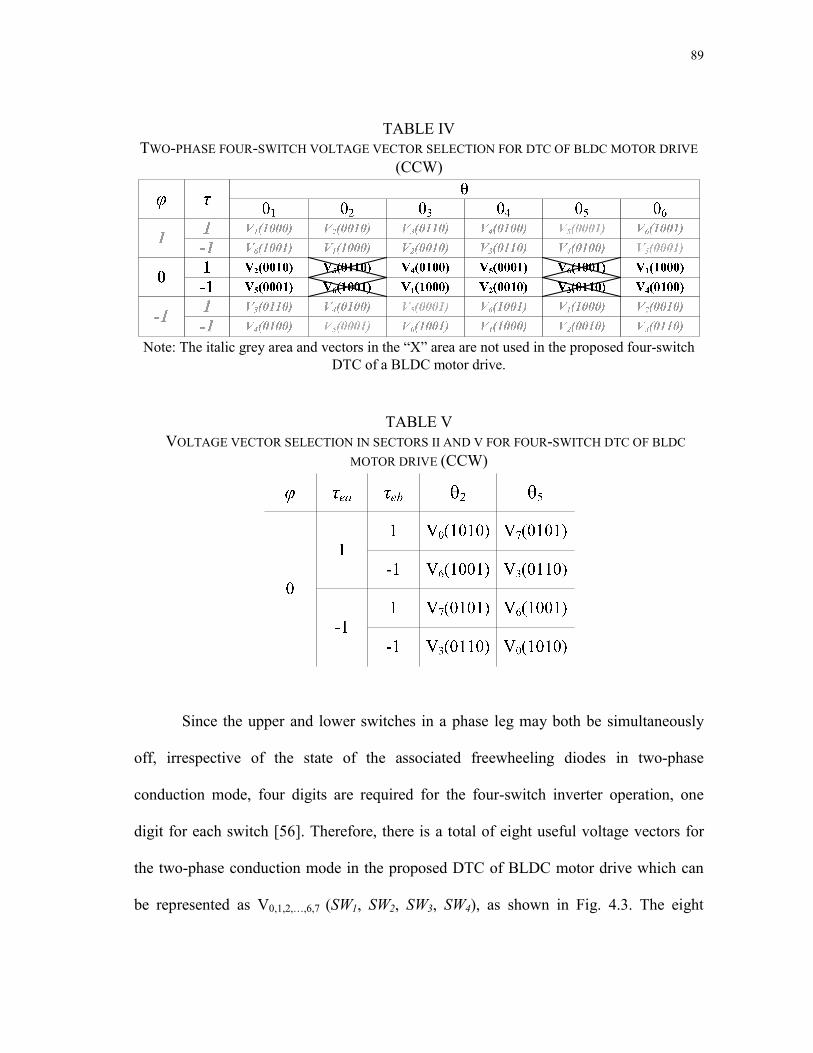
89
TABLE IV TWO-PHASE FOUR-SWITCH VOLTAGE VECTOR SELECTION FOR DTC OF BLDC MOTOR DRIVE
(CCW)
Note: The italic grey area and vectors in the “X” area are not used in the proposed four-switch DTC of a BLDC motor drive.
TABLE V
VOLTAGE VECTOR SELECTION IN SECTORS II AND V FOR FOUR-SWITCH DTC OF BLDC MOTOR DRIVE (CCW)
Since the upper and lower switches in a phase leg may both be simultaneously
off, irrespective of the state of the associated freewheeling diodes in two-phase
conduction mode, four digits are required for the four-switch inverter operation, one
digit for each switch [56]. Therefore, there is a total of eight useful voltage vectors for
the two-phase conduction mode in the proposed DTC of BLDC motor drive which can
be represented as V0,1,2,…,6,7 (SW1, SW2, SW3, SW4), as shown in Fig. 4.3. The eight

90
possible two-phase four-switch voltage vectors and current flow are depicted in Fig. 4.5.
Stationary reference frame (αβ–axes) representations of the eight voltage vectors with
respect to dc-link voltage and switching states of the semiconductor devices are derived
in Appendix D. The purpose of the hysteresis torque regulation is to shape the
quasisquare wave current within acceptable ripple band as the inverse top portion of the
actual back-EMF as shown in Fig. 4.2, therefore smoother torque can be obtained. In
Fig. 4.5, the solid lines represent current direction and the dotted lines show inactive
sections. The detailed switching sequence and torque regulation are showed in Fig. 4.6
for four-switch DTC of BLDC motor drive. The overall block diagram of the closed-
loop four-switch DTC scheme of a BLDC motor drive in the constant torque region is
represented in Fig. 4.7. The dotted area represents the stator flux linkage control part of
the scheme used only for comparison purpose. When the two switches in Fig. 4.7 are
changed from state 2 to state 1, flux control is considered in the overall system along
with torque control. In the two-phase conduction mode the shape of stator flux linkage
trajectory is ideally expected to be hexagonal, as illustrated with the straight dotted lines
in Fig. 4.3. However, the influence of the unexcited open-phase back-EMF causes each
straight side of the ideal hexagonal shape of the stator flux linkage locus to be curved
and the actual stator flux linkage trajectory tends to be more circular in shape, as shown
in Fig. 4.3 with solid curved lines [56]. In addition to the sharp changes, the curved
shape in the flux locus between two consecutive commutations complicates the control
of the stator flux linkage amplitude because it depends on the size of the sharp dips, and
the depth of the change may vary with sampling time, dc-link voltage, hysteresis
91
bandwidth, motor parameters especially the winding inductance, motor speed, snubber
circuit, and the amount of load torque.
Usually the overall control system of a BLDC motor drive includes three hall-
effect position sensors mounted on the stator 120 electrical degrees apart, as shown in
Fig. 4.3. These are used to provide good torque control if the back-EMF is ideally
trapezoidal because current commutation occurs only every 60 electrical degrees.
Nevertheless, using high resolution position sensors is quite useful if the back-EMF of
BLDC motor is not ideally trapezoidal. To achieve a more accurate torque estimation, in
general, for non-sinusoidal surface-mounted permanent magnet motors it is suggested
that (4.1) should be used. The derivative of the rotor αβ–axes fluxes obtained from (4.2)
over electrical position, which is described in (4.1), will cause problems mainly due to
the sharp dips at every commutation point. The actual values of αβ–axes back-EMF
constants kα and kβ vs. electrical rotor position θe can be created in the look-up table,
respectively with great precision depending on the resolution of the position sensor (for
example incremental encoder with 2048 pulses/revolution), therefore a good torque
estimation can be obtained in (4.1).
4.3.3. Torque Control Strategies of the Uncontrolled Phase-c
For direct torque control, Fig. 4.5(a) and (b) are not applicable due to the three-
phase conduction mode instead of a desired two-phase conduction. Modification in
PWM scheme presented in [70, 71] could be a solution if not for its tedious computation.
If torque or current is going to be controlled using hysteresis controllers, then those
voltage space vectors cannot be used in two-phase BLDC motor drive. On the other

92
hand, even though voltage vectors shown in Fig. 4.5(c) and (d) are two-phase
conductions through phase–a and –b, there will be always current trying to flow in
phase–c due to its back-EMF and the absence of switches controlling its current. As a
result, there will be a distorted current in phase–c as well as in phase–a and –b.
Therefore, voltage space vectors of phase–a and –b conduction can be difficult to
implement for BLDC motor drive unless some modifications are applied to overcome
the back-EMF effect of the phase–c in these conditions. Selecting the right switching
pattern to control the torque on phase–a and –b independently will reduce the distorted
currents on those phases and result in a smoother overall electromagnetic torque
production, which is shown in the simulations. Solution to the above phenomenon is
explained in detail below:
For BLDC motor with two-phase conduction, one of the phase torque should be
zero as shown in Table III. This can be achieved in Sectors 1, 3, 4 and 6 whereas in
Sectors 2 and 5 phase–c torque Tec is uncontrollable due to the split capacitors. In
Sectors 2 and 5, voltage vectors V3 and V6 cannot be directly used, instead phase torque
Tea and Teb should be individually controlled by properly selecting the S1, S2, S3, and S4
switches, such as if the rotor position resides in Sector 2 and the rotor rotates in CCW
direction then to increase the phase–a torque Tea S1 should be “0” and S2 is “1” and vice
versa to decrease the Tea. To increase the phase–b torque Teb S3 should be “0” and S4
should be “1” and vice versa to decrease the Teb. Reference torque value for those phase
torque should be half of the desired total reference torque Tearef = Tebref = Tref/2. This
special torque control phenomenon can be explained with the aid of the simplified

93
equivalent circuit in Fig. 4.6. Consequently, in Mode II and V only phase–a and –b
torque are controlled independently and therefore the Tec is tried to be kept at zero value.
This will eliminate the distorted torque problem on each phase in two-phase conduction
four-switch DTC of a BLDC motor drive.
The direction of the rotor is important to define the specific switching pattern. If
the rotor direction is CW, then the above claims are reversed, such as in Sector 2 to
increase the phase–a torque Tea S1 is “1” and S2 is “0” and vice versa for decrementing
the Tea. The same is true for the phase–b torque Teb.
Fig. 4.6. Individual phase–a and –b torque control, Tea and Teb , in Sectors 2 and 5.

94
Volta
ge S
ourc
e In
verte
r (V
SI)
Cur
rent
Sen
sors
Hys
tere
sis
Con
trolle
rs
Rot
orP
ositi
on
Elec
trom
agne
tic T
orqu
e Es
timat
ora b c
Cla
rke
Tran
sfor
mat
ion
V dc-
link
1
-1
10
-1
+-
+-
Stat
or F
lux
Link
age
Con
trol
BLD
CM
otor
()
3(
)(
)2
2em
es
es
PT
ki
ki
αα
ββ
θθ
=+
()
()dt
iR
V
dti
RV
ss
ss
sas
ss
∫∫−
=
−=
ββ
β
αα
ϕϕ2
2β
αϕ
ϕϕ
ss
s+
=
⎟⎟ ⎠⎞⎜⎜ ⎝⎛
−
αβ
ϕϕ ss1
tansθ
*(
)s
eϕ
θ
eθmθ
2P
∗emT
φ
SW1
SW2
SW3
SW4
T ea a
nd T
ebco
ntro
l1/
2
k a(θ
e)ia
k b(θ
e)ib
Two-
Phas
e Vo
ltage
Vec
tor
Sele
ctio
n Ta
ble
30
V2
V1
V3 V
4
V5
V6
V0
V7
Fig.
4.7
. Ove
rall
bloc
k di
agra
m o
f the
four
-sw
itch
two-
phas
e co
nduc
tion
DTC
of a
BLD
C m
otor
driv
e in
the
cons
tant
torq
ue re
gion
.

95
Another problem to overcome is eliminating the high torque ripples in Mode 2
and 5 where full dc-link is applied to the motor terminals compared to the other sectors
where only half and one third of the dc-link voltage is used. During Sectors 2 and 5
where the individual torque control is performed, bandwidth of the hysteresis torque
controllers are chosen about 1000 times less than the normal case which is used in
Sectors 1, 3, 4, and 6. Therefore, ripples in the current and eventually in the torque are
equalized during the entire electrical cycle.
Normally with four-switch inverter only half of the dc-link voltage is applied to
the motor terminals compared to the six-switch inverter. This problem can be overcome
by using voltage doubler half-bridge diode rectifier which can also be used for power
factor correction if two diodes are replaced with active power semiconductors such as
IGBTs and MOSFETs.
From the equivalent circuit given in Fig. 4.6, if phase–a and –b torque are
individually controlled as explained above, the influence of the back-EMF of the phase–
c can be blocked, there is no current flow in phase–c, therefore its torque (Tec) will be
almost zero. As a result, in Sectors 2 and 5, phase–a and –b torque should be controlled
independently, in other words switching signals at S1 (or S2) and S4 (or S3) should be
created individually making additional voltage vectors V0 and V7 which act as a zero
voltage vector at Sectors 2 and 5 in four-switch DTC of a BLDC motor drive scheme
using two phase conduction mode. Additional voltage vectors and their logic depending
on the errors of phase–a and –b torque are depicted in Table V.

96
At Sectors 2 and 5, complementary switches in both phase–a and –b legs cannot
be turned off at the same time as in V4 and V5, therefore inverse logic is applied in Fig.
4.6.
4.4. Simulation Results
The drive system shown in Fig. 4.7 has been simulated for various cases with and
without stator flux control, switch states 1 and 2, respectively in order to demonstrate the
validity of the proposed four-switch DTC of a BLDC motor drive scheme with two-
phase conduction.
To set the gating signals of the power switches easily and represent the real
conditions in simulation as close as possible the electrical model of the actual BLDC
motor with R-L elements and the inverter with power semiconductor switches
considering the snubber circuit are designed in Matlab/Simulink® using the SimPower
Systems toolbox.
The dead-time of the inverter and non ideal effects of the BLDC machine are
neglected in the simulation model. The sampling interval is 25 μs. The switching tables,
which are given in Table IV and V, are employed for the proposed DTC of the BLDC
motor drive. The magnitudes of the torque hysteresis band used in Sectors 1, 3, 4, and 6
τ1,3,4,6, and flux hysteresis band are 0.08 N·m and 0.001 Wb, respectively. Torque
hysteresis bandwidth in Sectors 2 and 5 τ2,5 is chosen as 0.08/1000 N·m to equal the high
frequency ripple width of both current and torque in one complete electrical cycle.
Figs. 4.8 and 4.9 show the simulation results of the uncontrolled open-loop stator
flux linkage locus when 0 N·m and 1.2835 N·m load torque are applied to the BLDC

97
motor with actual back-EMF waveforms, respectively. Steady-state speed control is
performed with an inner-loop torque control without flux control. Stator flux linkage is
estimated as an open-loop which is illustrated with dotted area in Fig. 4.7 without
connection of switch state 1 to the overall control scheme. As can be seen in Fig. 4.9
when the load torque level increases, more deep sharp changes are observed which
increase the difficulty of the flux control if it is used in the control scheme. The steady-
state speed is 30 mechanical rad/s and the dc-link voltage Vdc equals 80 2 V. Since the
speed is controlled a better open-loop circular flux trajectory is obtained. The overall
time for this simulation is 0.25 second.
Using the actual αβ–axes rotor flux linkages in (4.3) looks like the best solution
for a good stator flux reference similar to the DTC of a PMSM drive. Unlike BLDC
motor, in PMSM since both α– and β–axis motor back-EMFs are in sinusoidal shape,
constant stator flux linkage amplitude is obtained. However, for BLDC motor, unexcited
open-phase back-EMF effect on the flux locus and more importantly the size of the
sharp dips cannot easily be predicted to achieve a good stator flux reference in two-
phase conduction mode. Fig. 4.10 represents the steady-state estimated stator flux locus
whose reference obtained in (4.3) when back-EMF is not ideally a trapezoidal under full-
load (1.2835 N·m). The simulation time for this case is 3 seconds. The motor speed is 30
mechanical rad/s. Due to the distorted voltage and current, the estimation of stator flux
locus goes unstable as can be seen in Fig. 4.10.

98
-0.1 -0.05 0 0.05 0.1 0.15
-0.1
-0.05
0
0.05
0.1
0.15
Alfa-axis stator flux linkage (Wb)
Beta
-axi
s st
ator
flux
link
age
(Wb)
Fig. 4.8. Simulated open-loop stator flux linkage trajectory under the four-switch two-phase
conduction DTC of a BLDC motor drive at no load torque (speed + torque control).
-0.1 -0.05 0 0.05 0.1 0.15
-0.1
-0.05
0
0.05
0.1
0.15
Alfa-axis stator flux linkage (Wb)
Beta
-axi
s st
ator
flux
link
ages
(Wb)
Fig. 4.9. Simulated open-loop stator flux linkage trajectory under the four-switch two-phase
conduction DTC of a BLDC motor drive at 1.2835 N·m load torque (speed + torque control).
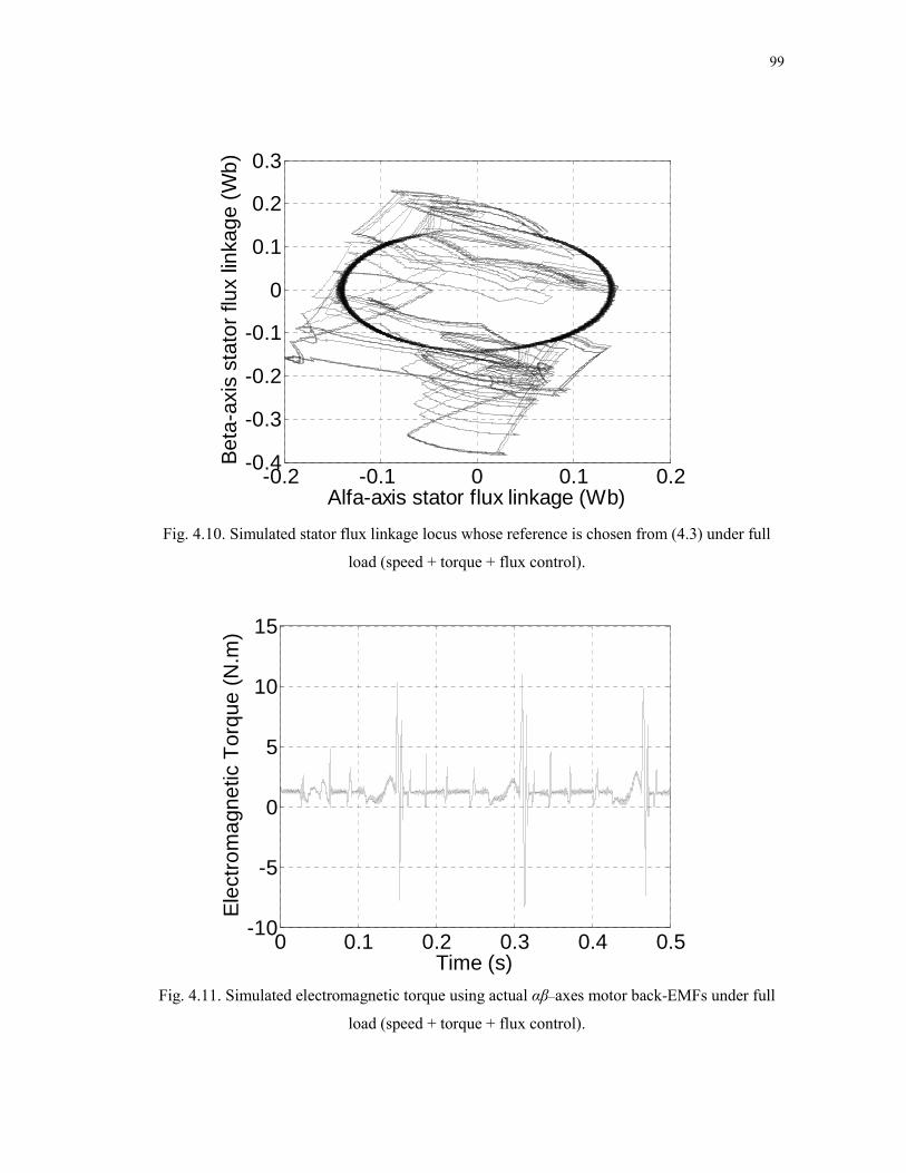
99
-0.2 -0.1 0 0.1 0.2-0.4
-0.3
-0.2
-0.1
0
0.1
0.2
0.3
Alfa-axis stator flux linkage (Wb)
Beta
-axi
s st
ator
flux
link
age
(Wb)
Fig. 4.10. Simulated stator flux linkage locus whose reference is chosen from (4.3) under full
load (speed + torque + flux control).
0 0.1 0.2 0.3 0.4 0.5-10
-5
0
5
10
15
Time (s)
Elec
trom
agne
tic T
orqu
e (N
.m)
Fig. 4.11. Simulated electromagnetic torque using actual αβ–axes motor back-EMFs under full
load (speed + torque + flux control).

100
Instability in the torque is observed in Fig. 4.11 where huge torque transients
occur mainly at the commutation points. During Sectors 2 and 5 the torque estimation
results in even larger transients which are unacceptable in real conditions. The reason of
instability in the torque estimation is because of considering the flux control with a large
reference flux to estimated flux ratio or vice versa during especially commutation
periods in two-phase controlled four-switch DTC of a BLDC motor drive. There should
be exact flux amplitude to be given as a reference flux value including sharp changes at
every commutation point and curved shape between those commutation points, then
appropriate flux control can be obtained without losing the torque control. However, to
predict all these circumstances to generate a flux reference is a cumbersome work which
is unnecessary in the constant torque region.
Although the phase currents illustrated in Fig. 4.12 seem to be stable only until
the second commutation point so as the electromagnetic torque as shown in Fig. 4.11.
Then, the currents become unstable exceeding the peak current of 24 A due to the huge
mismatch of the reference flux versus estimated flux in the two-phase conduction DTC
of BLDC motor drive scheme. Once the currents go unstable the current dependant
torque estimation is also affected enormously as can be seen in Fig. 4.11.

101
0 0.1 0.2 0.3 0.4 0.5
-60
-40
-20
0
20
40
60
Time (s)
abc
fram
e ph
ase
curr
ents
(A)
Fig. 4.12. Simulated abc frame phase currents when stator flux reference is obtained from (4.3)
under full load (speed + torque + flux control).
Figs. 4.13 and 4.14 show abc frame phase currents and electromagnetic torque,
respectively under only torque control when the actual phase back-EMFs are considered
in the simulation. Due to the individual torque control at Sectors 2 and 5 ripples on
phase–c current during zero-crossing points are clearly visible in Fig. 4.13. The torque
ripples of phase–c as a consequence of individual torque control scheme are not large
enough to distort the torque estimation as illustrated with grey circle in Fig. 4.14. High-
frequency current and torque ripples observed in Figs. 4.13 and 4.14 are due to the high
dc-link voltage, high sampling time, low winding inductance, high torque hysteresis
bandwidth, etc. Those ripples can be minimized by selecting the proper values of dc-link
voltage and hysteresis band size. Once the dc-link voltage is reduced to obtain less high-

102
frequency ripples the hysteresis band size τ1,3,4,6 of Sectors 1, 3, 4, and 6 should also be
decreased accordingly to get an equal ripple size in one complete electrical cycle for
both currents and torque. The size of the torque hysteresis bandwidth at Sectors 2 and 5
τ2,5 is still kept as τ1,3,4,6 /1000 N·m. In Fig. 14, reference torque is 0.51 N·m and the load
torque is 0.5 N·m, thereby steady-state speed is kept around 30 electrical rad/s for a
better circular flux locus. If high resolution position sensor such as incremental encoder
is used instead of the three hall-effect sensors, low-frequency torque oscillations can be
minimized by using (4.1), as shown in Fig. 4.14. In (4.1), the exact shapes of phase
back-EMF constants are obtained offline and transformed to αβ–axes. Thus, the product
of the real back-EMF constant values by the corresponding αβ–axes currents, and
number of pole pairs provide the exact values of the α– and β–axis torque, respectively.
0 0.1 0.2 0.3 0.4 0.5-6
-4
-2
0
2
4
6
Time (s)
abc
fram
e ph
ase
curr
ents
(A)
Phase A Phase B Phase C
Fig. 4.13. Simulated abc frame phase currents when just torque is controlled without flux control
under 0.5 N·m load using actual back-EMFs (reference torque is 0.51 N·m).

103
0 0.2 0.4 0.6 0.8 1-0.5
0
0.5
1
1.5
Time (s)
Elec
trom
agne
tic to
rque
(N.m
)
Fig. 4.14. Simulated electromagnetic torque when just torque is controlled without flux control
under 0.5 N·m load using actual back-EMFs (reference torque is 0.51 N·m).
4.5. Experimental Results
The feasibility and practical features of the proposed four-switch DTC of a
BLDC motor drive scheme have been evaluated using an experimental test-bed, shown
in Fig. 4.15. The proposed control algorithm is digitally implemented using the eZdspTM
board from Spectrum Digital, Inc. based on TMS320F2812 DSP, as shown in Fig
4.15(a). In Fig. 4.15(b), the BLDC motor whose parameters are given in the Appendix A
is coupled to the overall system.
Phase-c torque Tec effect

104
(a)
(b)
Fig. 4.15. Experimental test-bed. (a) Four-switch inverter and DSP control unit. (b) BLDC motor
coupled to dynamometer and position encoder (2048 pulse/rev).
BLDC Motor
Hysteresis Brake
Position Encoder
SEMIKRON Inverter
Phase-c to center
eZdsp2812

105
In this section, transient and steady-state torque and current responses of the
proposed four-switch two-phase conduction DTC scheme of a BLDC motor drive are
demonstrated experimentally under 0.5 N·m load torque condition. The experimental
results are obtained from the datalog (data logging) module in the Texas Instruments
Code Composer StudioTM IDE software.
Fig. 4.16 illustrates the experimental results of the torque and abc frame phase
currents when only torque control is performed using (4.1).. In Fig. 4.16, the reference
torque is suddenly increased 25 percent from 0.51 N·m to 0.6375 N·m at 0.05 s under 0.5
N·m load torque. The sampling time is chosen as 25 μs, hysteresis bandwidth is 0.05
N·m for Sectors 1, 3, 4, and 6, for Sectors 2 and 5 it is selected as 0.0005 N·m to
equalize the high-frequency ripple widths with the ones in the other sectors, the dead-
time compensation is included, and the dc-link voltage is set to Vdc = 80 2 V. As it can
be seen in Fig. 4.16, when the torque is suddenly increased the current amplitudes also
increase and fast torque response is achieved. The high frequency ripples observed in the
torque and current are related to the sampling time, hysteresis bandwidth, winding
inductance, and dc-link voltage. Those ripples can be minimized by properly selecting
the dc-link voltage and torque hysteresis band size. The steady-state experimental results
are well in accordance with the simulation results obtained in Figs. 4.13 and 4.14. Since
only the torque is controlled without speed control, the time range of control system
under transient state is selected short. The motor speeds up to a very large value if the
motor is run longer under only torque control.

106
abc
fram
e cu
rrent
s [2
A/d
iv]
Time [16.07 ms/div]
Electrom
agnetic torque [0.5 N.m
/div]
Fig. 4.16. Top: Steady-state and transient experimental electromagnetic torque in per-unit under
0.5 N·m load torque (0.5 N·m/div). Bottom: Steady-state and transient experimental abc frame
phase currents (2 A/div) and time base: 16.07 ms/div.
4.6. Conclusion
This study has successfully demonstrated application of the proposed four-switch
two-phase conduction direct torque control (DTC) scheme for BLDC motor drives in the
constant torque region. A look-up table for the two-phase voltage selection is designed
to provide faster torque response. In addition, for effective torque control, a novel
switching pattern incorporating with the voltage vector look-up table is developed and
implemented for the two-phase four-switch DTC of a BLDC motor drive to produce the
desired torque characteristics. Furthermore, to eliminate the low-frequency torque
oscillations caused by the non-ideal trapezoidal shape of the actual back-EMF waveform
Phase–c torque Tec effect

107
of the BLDC motor, a pre-stored back-EMF versus electrical rotor position look-up table
is designed and used in the torque estimation.
Compared to the three phase DTC technique, this approach eliminates the flux
control and only torque is considered in the overall control system. Three reasons are
given for eliminating the flux control. First, since the line-to-line back-EMF including
the small voltage drops is less than the dc-link voltage in the constant torque region there
is no need to control the flux amplitude. Second, with the two-phase conduction mode
sudden sharp dips in the stator flux linkage locus occur that complicate the control
scheme. The size of these sharp dips is unpredictable. Third, regardless of the stator flux
linkage amplitude, the phase currents tend to match with the flat top portion of the
corresponding trapezoidal back-EMF to generate constant torque. The simulation and
experimental results show that it is possible to achieve two-phase conduction DTC of a
BLDC motor drive using four-switch inverter.

108
CHAPTER V
SENSORLESS DIRECT TORQUE AND INDIRECT FLUX CONTROL OF
BRUSHLESS DC MOTOR WITH NON-SINUSOIDAL BACK-EMF
5.1. Introduction
The permanent magnet synchronous motor (PMSM) and brushless dc (BLDC)
motor drives are used extensively in several high-performance applications, ranging
from servos to traction drives, due to several distinct advantages such as high power
density, high efficiency, large torque to inertia ratio, and simplicity in their control.
In many applications, obtaining a low-frequency ripple-free torque and
instantaneous torque and even flux control are of primary concern for BLDC motors
with non-sinusoidal back-EMF. If the actual back-EMF of a BLDC motor is not ideal
trapezoidal having a 120 degrees flat top, control scheme with discrete position sensing
will generate low-frequency torque pulsations depending on the shape of the back-EMF.
A great deal of study has been devoted to the current and torque control methods
employed for BLDC motor drives to minimize the torque pulsations mainly caused by
commutation and non-ideal shape of back-EMF. One of the most popular approaches is
a generalized harmonic injection approach by numerical optimization solutions to find
out optimal current waveforms based on back-EMF harmonics to minimize mutual and
cogging torque [73]–[78], [47]–[49]. In [47], it is shown that torque ripple can be
minimized by appropriately selecting the current harmonics to eliminate both excitation
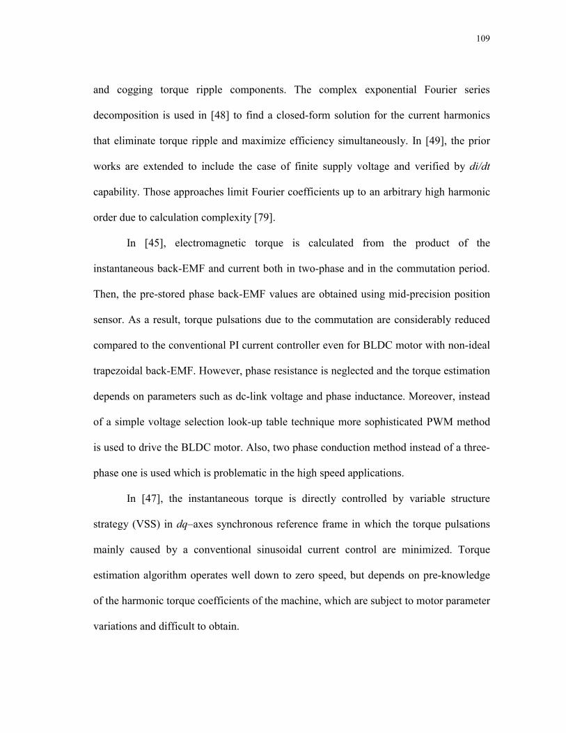
109
and cogging torque ripple components. The complex exponential Fourier series
decomposition is used in [48] to find a closed-form solution for the current harmonics
that eliminate torque ripple and maximize efficiency simultaneously. In [49], the prior
works are extended to include the case of finite supply voltage and verified by di/dt
capability. Those approaches limit Fourier coefficients up to an arbitrary high harmonic
order due to calculation complexity [79].
In [45], electromagnetic torque is calculated from the product of the
instantaneous back-EMF and current both in two-phase and in the commutation period.
Then, the pre-stored phase back-EMF values are obtained using mid-precision position
sensor. As a result, torque pulsations due to the commutation are considerably reduced
compared to the conventional PI current controller even for BLDC motor with non-ideal
trapezoidal back-EMF. However, phase resistance is neglected and the torque estimation
depends on parameters such as dc-link voltage and phase inductance. Moreover, instead
of a simple voltage selection look-up table technique more sophisticated PWM method
is used to drive the BLDC motor. Also, two phase conduction method instead of a three-
phase one is used which is problematic in the high speed applications.
In [47], the instantaneous torque is directly controlled by variable structure
strategy (VSS) in dq–axes synchronous reference frame in which the torque pulsations
mainly caused by a conventional sinusoidal current control are minimized. Torque
estimation algorithm operates well down to zero speed, but depends on pre-knowledge
of the harmonic torque coefficients of the machine, which are subject to motor parameter
variations and difficult to obtain.

110
Torque coefficients in [47] are updated using an on-line recursive least square
estimator in [48], however it is computationally intensive and difficult to implement
because it requires differentiation of the motor current. Real-time harmonics flux
estimator to calculate the sixth-harmonic current that must be injected to cancel the
sixth- and twelfth-harmonic pulsating torque components rather than depending on
stored coefficients is reported in [49]. However, obtaining those harmonics is a quite
complicated task. Moreover, instead of a simple voltage vector selection method more
complicated SVPWM technique is used to drive the motor. Since the torque is not
controlled directly, fast torque response cannot be achieved. Also, rotor speed is
measured by an expensive resolver and back-EMF harmonics higher than sixth order are
neglected for simplification resulting in a reduction of the accuracy in the estimation
algorithms in which the knowledge of the fundamental peak magnet flux is required.
In [46], the disadvantages observed in [47]–[49] are claimed to be improved by
proposing a new instantaneous torque control. It is based on the model reference
adaptive system (MRAS) technique and the torque is calculated by using the estimated
flux and measured current. Then, the torque is instantaneously controlled by the torque
controller using the integral variable structure control (IVSC) and the space-vector
pulse-width modulation (SVPWM). Thus, good steady-state performance and switching
characteristics are obtained. Compared to LSM, this technique does not require the
differentiation of the motor current and the estimating performance is less sensitive to
the measurement noise. Torque and speed pulsations are effectively reduced.
Nevertheless, this technique increases the complexity of the control system.

111
In [50], predetermination of optimal current wave shapes using Park like dq–axes
reference frame is obtained by adding some harmonics to the fundamental current to
cancel specific torque harmonic components. However, these optimal current references
are not constant and require very fast controllers especially when the motor operates at
high speed. Moreover, the bandwidth of the classical proportional plus integral (PI)
controllers does not allow tracking all of the reference current harmonics.
Problems in [50] are claimed to be solved in [51] such that a new torque control
strategy using the ba–ca reference frame is proposed in which easily accessible line-to-
line back-EMFs are measured and stored in a look-up table. Smooth and maximum
torque is obtained, however this technique presents a steady-state torque error compared
to the dq–axes reference frame scheme in [50] and the motor is driven by digital scalar
modulation technique which operates like a SVPWM, therefore a more complicated
control is inevitable.
Since the Park Transformation and its extensions proposed in [50] do not
linearize completely the non-linear model of the machine, state feedback linearization
technique is applied in order to obtain the desired high performance torque control in
[52]. Additionally, more tedious computations are needed to be performed compared to
[50], which complicates the real-time implementation of the control strategy.
The optimum current excitation methods, considering the unbalanced three-phase
stator windings as well as non-identical and half-wave asymmetric back-EMF
waveforms in BLDC motor, are reported in [43], [79]. These methods avoid the
complicated harmonic coefficient calculation based on the optimization approach. In

112
[43], each phase back-EMF versus rotor position data is stored in a look-up table. Then,
they are transformed to the dq–axes synchronous reference frame. The d–axis current is
assumed to be zero and the q–axis current is obtained from the desired reference torque,
motor speed, and the q–axis back-EMF. Consequently, inverse park transformation is
applied to the dq–axes currents to obtain the abc frame optimum reference current
waveforms. Minimum torque ripple and maximum efficiency are achieved at low speeds
for a BLDC motor. However, three hysteresis current controllers with PWM generation,
which increases the complexity of the drive, are used to drive the BLDC motor. Several
transformations are required in order to get the abc frame optimum reference current
waveforms. These transformations complicate the control algorithm and the scheme
could not directly control the torque, therefore fast torque response cannot be achieved.
Three offline measured back-EMF waveforms are needed for the torque estimation.
Moreover, stator flux is not controlled, therefore high speed applications are not
possible. In [79], an alternative simple and straightforward solution to eliminate torque
ripple in BLDC machines is presented. This method is not dq based approach as in [43]
and hence do not require the dq transformation which increases the complexity of the
control system. The copper loss minimization strategy is also utilized. However, the pre-
measured three line-to-neutral back-EMF waveforms are needed and three phase
currents are controlled instead of dq–axes currents. Therefore, field-weakening operation
cannot easily be performed.
In [41, 80], the method of multiple reference frames is employed in the
development of a state variable model for BLDC drives with non-sinusoidal back-EMF

113
waveforms. This model has the desirable features of being valid for transient and steady-
state analysis as well as having state variables that are constant in the steady-state. This
method results in the same torque capability during constant torque region as in the six-
step current control technique. Also, the same level of controllability as in the case of
sinusoidal PMSM over the flux weakening region and regeneration operation compared
to the conventional six-step BLDC drive system is achieved [41]. However, the method
involves tedious algorithms which increase the complexity of the control system.
Moreover, in [41], to determine the right d–axis current in flux-weakening region the
high order d–axis harmonic current values are required which are quite difficult to
obtain. Also, the back-EMF is assumed to be ideal trapezoidal and its harmonics higher
than seventh order are neglected which results in a reduction of the accuracy in the
overall system.
Direct torque control (DTC) scheme was first proposed by Takahashi [53] and
Depenbrock [54] for induction motor drives in the mid 1980s. More than a decade later,
in the late 1990s, DTC techniques for both interior and surface-mounted synchronous
motors (PMSM) were analyzed [55]. More recently, application of DTC scheme is
extended to BLDC motor drives to minimize the low-frequency torque ripples and
torque response time as compared to conventional PWM current controlled BLDC motor
drives [56, 72]. In [56] and [72], the voltage space vectors in a two-phase conduction
mode are defined and a stationary reference frame electromagnetic torque equation is
derived for surface-mounted permanent magnet synchronous machines with non-
sinusoidal back-EMF (BLDC, and etc.). It is shown in [72] that only electromagnetic

114
torque in the DTC of BLDC motor drive under two-phase conduction mode can be
controlled. Flux control is not trivial due to the sharp changes whose amplitudes are
unpredictable depending on several factors such as load torque, dc-link voltage, winding
inductance, etc.
In this chapter, the torque control method presented in [56] and [72] is adapted to
the position sensorless direct torque control scheme for three-phase conduction BLDC
motor by using the new Line-to-Line Park Transformation which forms a 2x2 matrix
instead of the conventional 2x3 matrix. Therefore, rather than three line-to-neutral back-
EMF waveforms which are not directly available in the motor easily accessible two line-
to-line back-EMF waveforms (eba and eca) are obtained offline and converted to the
electrical rotor position dependant line-to-line back-EMF constants (kba(θe) and kca(θe)).
Then, they are converted to dq–axes equivalents (kd(θe) and kq(θe)) using Line-to-Line
Park Transformation. dq–axes back-EMF constants versus electrical rotor position data
(kd(θe) and kq(θe)) are stored in a look-up table for the torque estimation. As opposed to
the prior two-phase conduction methods, this DTC technique can control both torque and
stator flux of the BLDC motor simultaneously, therefore field-weakening operation is
possible. The electrical rotor position is estimated using winding inductance and
stationary reference frame stator flux linkages and currents. The proposed sensorless
DTC method controls the torque directly and stator flux amplitude indirectly using d–
axis current. Since the stator flux is estimated, position sensorless DTC of BLDC motor
drive scheme can be achieved. Unlike those for motor with sinusoidal back-EMFs,
optimal current references for a non-sinusoidal back-EMF motor (BLDC) in the
115
synchronous reference frame are not constant, therefore current wave shapes require
very fast controllers in particular at high speed. Classical bandwidth of the controller
(such as proportional-integral–PI) does not allow tracking all of the reference current
harmonics [51]. Since the hysteresis controllers used in the proposed DTC scheme are
not fast controllers like PI, they can easily regulate not only constant but also the varying
references (torque and flux). Simulation and experimental results are presented to
illustrate the validity and effectiveness of the sensorless three-phase conduction DTC of
a BLDC motor drive.
5.2. The Proposed Line-to-Line Clarke and Park Transformations in 2x2 Matrix
Form
5.2.1. Conventional Park Transformation for Balanced Systems
In 1929, R. H. Park [81] introduced a new approach to electric machine analysis.
In [81], Park Transformation is developed such that stator quantities of a synchronous
machine are transformed onto a dq reference frame that is fixed to the rotor, with the
positive d–axis aligned with the magnetic axis of the field winding and the positive q–
axis is defined as leading the positive d–axis by π/2 [82]. Therefore, from the rotor point
of view, all the variables can be observed as constant values. As a result, this
transformation has created a revolutionary idea that all the time varying quantities in a
polyphase machine are converted to orthogonal two-phase equivalents which are
controllable constant values. For the balanced n–phase to two-phase case, Park
Transformation can be expressed excluding the zero-sequence term as

116
[ ][ ]123( )dq nX T Xθ⎡ ⎤ =⎣ ⎦ … (5.1)
where
[ ]cos cos cos ( 1)
2 2 22( )3
sin sin sin ( 1)2 2 2
P P P nT
P P P n
θ θ ξ θ ξθ
θ θ ξ θ ξ
⎡ ⎤⎛ ⎞ ⎛ ⎞ ⎛ ⎞− − −⎜ ⎟ ⎜ ⎟ ⎜ ⎟⎢ ⎥⎝ ⎠ ⎝ ⎠ ⎝ ⎠⎢ ⎥=⎢ ⎥⎛ ⎞ ⎛ ⎞ ⎛ ⎞− − −⎢ ⎥⎜ ⎟ ⎜ ⎟ ⎜ ⎟
⎝ ⎠ ⎝ ⎠ ⎝ ⎠⎣ ⎦
…
… (5.2)
The coefficient 2/3 in (5.2) is used to make the transformation power invariant
and θ is the electrical angle between adjacent magnetic axes of the uniformly distributed
n–phase windings. The transformation angle θ is the angular displacement of the rotor
reference frame.
The more general balanced three-phase to two-phase Park Transformation
without a zero-sequence term X0 can be expressed as
[ ]( )a
db
qc
XX
T XX
Xθ
⎡ ⎤⎡ ⎤ ⎢ ⎥=⎢ ⎥ ⎢ ⎥⎣ ⎦ ⎢ ⎥⎣ ⎦
(5.3)
where the dq transformation matrix [ ]( )T θ is defined as
[ ] ( ) ( )( ) ( )
cos cos 2 / 3 cos 2 / 32( )sin sin 2 / 3 sin 2 / 33
Tθ θ π θ π
θθ θ π θ π
− +⎡ ⎤= ⎢ ⎥− +⎣ ⎦
(5.4)
In (5.4), q–axis is lagging the d–axis by π/2. Another method uses a qd
transformation in which the q–axis leads the d–axis and the transformation angle θ is
between the q–axis and the a–axis instead of d–axis and a–axis as in (5.4) [82].
However, both methods will produce the same results.

117
5.2.2. The Proposed Line-to-Line Clarke and Park Transformations for Balanced
Systems
Since the balanced systems in dq–axes reference frame do not require a zero
sequence term, first the Line-to-Line Clarke Transformation from the balanced three-
phase quantities is derived and, then the Line-to-Line Park Transformation forming a
2x2 matrix instead of a 2x3 matrix as in (5.4) for three-phase systems can be obtained in
the followings:
Line-to-Line Clarke Transformation which requires only two input variables (bc
and ca frame) can be obtained from conventional abc frame version as follows:
First, classical Clarke Transformation, abc to αβ frame, is derived by replacing
zero with the transformation angle θ in (5.4) and the matrix form is obtained as
a
b
c
XX
T XX
X
ααβ
β
⎡ ⎤⎡ ⎤ ⎢ ⎥⎡ ⎤=⎢ ⎥ ⎣ ⎦ ⎢ ⎥⎣ ⎦ ⎢ ⎥⎣ ⎦
(5.5)
where
1 112 2 23 3 30
2 2
Tαβ
⎡ ⎤− −⎢ ⎥⎡ ⎤ ⎢ ⎥=⎣ ⎦ ⎢ ⎥−⎢ ⎥⎣ ⎦
(5.6)
Xα and Xβ are the stationary reference frame components, and Xa, Xb, and Xc are
the abc frame components. In (5.5), X represents machine variables such as currents,
voltages, flux linkages, back-EMFs, and etc.
If Xα and Xβ are expanded and algebraically manipulated, the line-to-line
representations of Xα and Xβ in ba–ca reference frame are attained respectively as

118
2
3 3 3a b c a b a c ba caX X X X X X X X XX α− − − + − − −
= = = (5.7)
and
( ) ( ) ( )3 3 33 3 3b c b a a c ba caX X X X X X X X Xβ = − = − + − = − (5.8)
where ba b aX X X= − and ca c aX X X= − .
Using the results obtained in (5.7) and (5.8), Xα and Xβ can be rewritten in matrix
form as
[ ] baLL
ca
X XT
X Xα
β
⎡ ⎤ ⎡ ⎤=⎢ ⎥ ⎢ ⎥
⎣ ⎦⎣ ⎦ (5.9)
where
[ ]
1 13 33 3
3 3
LLT
⎡ ⎤− −⎢ ⎥⎢ ⎥=⎢ ⎥−⎢ ⎥⎣ ⎦
(5.10)
As it can be seen in (5.10) that original Clarke Transformation forming a 2x3
matrix given in (5.8) excluding the zero-sequence term can be simplified to a 2x2 matrix
which requires only two input variables.
Second, to obtain abc to ba–ca frame transformation the inverse of the Clarke
Transformation matrix Tαβ⎡ ⎤⎣ ⎦ given in (5.6) is required. Since the zero-sequence term is
removed, Tαβ⎡ ⎤⎣ ⎦ is not square anymore, but it is still singular and therefore pseudo-
inverse can be found in the followings:
( ) 1T TT T T Tαβ αβ αβ αβ
−+⎡ ⎤ ⎡ ⎤ ⎡ ⎤ ⎡ ⎤=⎣ ⎦ ⎣ ⎦ ⎣ ⎦ ⎣ ⎦ (5.11)

119
where Tαβ
+⎡ ⎤⎣ ⎦ and
TTαβ⎡ ⎤⎣ ⎦ are the pseudo-inverse and transpose of the original Clarke
Transformation matrix Tαβ⎡ ⎤⎣ ⎦ , respectively.
Abc to ba–ca transformation matrix can be derived using the pseudo-inverse
matrix Tαβ
+⎡ ⎤⎣ ⎦ , original Clarke Transformation matrix Tαβ⎡ ⎤⎣ ⎦ and Line-to-Line Clarke
Transformation matrix [ ]LLT as follows:
[ ]a
bab LL
cab
XX
T T X T TX
Xαβ αβ αβ
+ +⎡ ⎤
⎡ ⎤⎢ ⎥⎡ ⎤ ⎡ ⎤ ⎡ ⎤= ⎢ ⎥⎣ ⎦ ⎣ ⎦ ⎣ ⎦⎢ ⎥ ⎣ ⎦⎢ ⎥⎣ ⎦
(5.12)
hence
1 13 3
2 13 31 23 3
aba
bca
b
XX
XX
X
⎡ ⎤− −⎢ ⎥⎡ ⎤ ⎢ ⎥
⎡ ⎤⎢ ⎥ ⎢ ⎥= − ⎢ ⎥⎢ ⎥ ⎢ ⎥ ⎣ ⎦⎢ ⎥ ⎢ ⎥⎣ ⎦⎢ ⎥−⎢ ⎥⎣ ⎦
(5.13)
Then, the ba–ca to dq frame Line-to-Line Park Transformation can be written
using (5.4) in (5.13) as
[ ]
1 13 3
2 1( )3 31 23 3
d ba
q ca
X XT
X Xθ
⎡ ⎤− −⎢ ⎥⎢ ⎥⎡ ⎤ ⎡ ⎤⎢ ⎥= −⎢ ⎥ ⎢ ⎥⎢ ⎥ ⎣ ⎦⎣ ⎦ ⎢ ⎥⎢ ⎥−⎢ ⎥⎣ ⎦
(5.14)
After (5.14) is expanded and simplified using some trigonometric equivalence,
the following 2x2 Line-to-Line Park Transformation matrix form is obtained:

120
( ) ( )( ) ( )
sin / 6 sin / 62cos / 6 cos / 63
d ba
q ca
X XX X
θ π θ πθ π θ π− − +⎡ ⎤⎡ ⎤ ⎡ ⎤
= ⎢ ⎥⎢ ⎥ ⎢ ⎥− − + ⎣ ⎦⎣ ⎦ ⎣ ⎦ (5.15)
5.3. The Proposed Sensorless DTC of BLDC Drive Using Three-Phase Conduction
5.3.1. Principles of the Proposed Method
In this work, indirect torque control method of BLDC motor explained in [43] is
extended to a direct torque and indirect flux control technique which is suitable for
sensorless and field-weakening operations. The proposed method transforms abc frame
quantities to dq frame ones using the new 2x2 Line-to-Line Park Transformation matrix.
Rather than three measured phase back-EMFs which are used in [43], in the proposed
balanced system only two electrical rotor position dependant back-EMF constants (kd(θe)
and kq(θe)) are required in the torque estimation algorithm. Since the numbers of input
variables (current and back-EMF) are reduced from three to two, much simpler Park
Transformation can be used as given in (5.15). Therefore, the amount of multiplications
and sine/cosine functions are minimized.
Unlike previous two-phase conduction DTC of BLDC motor drive techniques
which are proposed in [56, 72], this method uses DTC technique with three-phase
conduction, therefore field-weakening operation as well as a much simpler position
sensorless technique can easily be achieved. Compared to the two-phase conduction
DTC scheme, this DTC method differs by its torque estimation and voltage vector
selection table which is similar to the one used for DTC of PMSM drives explained in
[10]. Although stator flux estimation algorithm in both methods (two-phase and three-
phase conduction) is the same due to the similar machine model in which the back-EMF

121
shape separates the two from each other, in two-phase conduction scheme the stator flux
amplitude is uncontrollable. Since the proposed technique adopts three-phase
conduction, there is a possibility to control the stator flux amplitude without
commutation issue, therefore field-weakening and sensorless operations which involve
back-EMF estimation can easily be performed. Moreover, this DTC method controls the
voltage vectors directly from a simple look-up table depending on the outcome of
hysteresis torque and indirect flux controllers, thus the overall control is much simpler
and faster torque response can be achieved compared to the conventional PWM control
techniques.
Unless the harmonic components of field distribution and inductance variation
are considered, the synchronously rotating dq reference frame analysis is no longer valid
for BLDC motors with non-sinusoidal back-EMF because the stator to rotor mutual
inductance does not vary sinusoidally [43]. Since the proposed DTC of BLDC motor
drive method does not consider performing a modeling and simulation of the motor itself
as in the Fourier analysis and multiple reference frame operations, the dq reference
frame approach can easily be adopted to the DTC scheme to obtain a low-frequency
ripple free torque based on the minimum input power.
Most of the previous work to eliminate low-frequency torque ripples for BLDC
motors assumed that the neutral point of the motor is available. Measurement of the
three-phase back-EMFs requires access to the neutral point connection of the stator. In
most cases, this represents extra cost and inconvenience to the motor installation.

122
Especially, in Y-connected systems, the neutral point is generally not available.
Therefore, it is not practical and cumbersome to extract the neutral point [43].
For PMSM with non-sinusoidal back-EMF constituting odd harmonics, stator
flux linkages rdsϕ and r
qsϕ in the dq–axes rotor reference frame can be obtained,
respectively as [47]
r r r
ds ds ds dqs qs dsf fL i L i L iϕ = + + (5.16)
r r r
qs qs qs qds ds qsf fL i L i L iϕ = + + (5.17)
where dqsL and qdsL are the mutual inductances between d– and q–axis, respectively.
rdsi and r
qsi , dsL and qsL are the d– and q–axis currents and inductances, respectively.
dsfL and qsfL are the mutual inductances between dq–axes and permanent magnet,
respectively. fi is the equivalent current generated by PM.
All the machine inductances given in (5.16) and (5.17) can be written
considering the flux harmonics which are multiple of six as [43]
0 6 12cos 6 cos12ds ds ds r ds rL L L Lθ θ= + + + (5.18)
6 12sin 6 cos12dqs dqs r dqs rL L Lθ θ= + + (5.19)
6 12sin 6 cos12dsf dsf dsf r dsf rL L L Lθ θ= + + + (5.20)
0 6 12cos 6 cos12qs qs qsf r qsf rL L L Lθ θ= + + + (5.21)
6 12sin 6 sin12qds qds r qds rL L Lθ θ= + + (5.22)
6 12cos 6 cos12qsf qsf qsf r qsf rL L L Lθ θ= + + + (5.23)

123
As it can be seen in (5.18)–(5.23) that the inductances in the rotor reference
frame are not constant as in pure sinewave machines and represented by the fundamental
term and/or multiple of six because the third harmonic and its multiples are internally
cancelled out in the Y-connected three-phase systems and from the remaining
harmonics, 5th and 7th harmonics transform into 6th harmonics, 11th and 13th harmonics
transform into 12th harmonics, and so on.
The motors with high-coercive PM material, the effects of the inductance
harmonics in the stator winding can be negligible for the torque pulsation which is
mainly produced by the flux harmonics in the PM. Therefore, for machines with surface-
mount magnet rotor (BLDC) it can be assumed that dsL and qsL are constant, i.e.,
0 0ds qs ds qs sL L L L L= = = = , and 0dqs qdsL L= = Thus, stator flux linkages in rotor dq
reference frame given in (5.16) and (5.17) can be rewritten as
r r
ds ds ds dsf fL i L iϕ = + (5.24)
r r
qs qs qs qsf fL i L iϕ = + (5.25)
If the second term on the right hand side in (5.24) and (5.25) is expanded into the
time-varying equivalence, the following equations are obtained:
( ) ( )6 1 6 11
cos 6r rds s ds r n n r r
nL i K K nϕ ϕ θ ϕ
∞
− +=
′ ′= + − +∑ (5.26)
( ) ( )6 1 6 11
sin 6r rqs s qs r n n r
nL i K K nϕ ϕ θ
∞
− +=
′= + +∑ (5.27)

124
where rϕ ′ is the peak value of the fundamental rotor magnetic flux linkage, the
coefficients 6 1nK − and 6 1nK + represent the odd harmonics of the phase back-EMF other
than the third and its multiples. 6 1nK − equals ( ) ( )3sin 6 1 / 6 1 sinn nα α⎡ ⎤⎡ ⎤− −⎣ ⎦ ⎣ ⎦ , and
6 1nK + is ( ) ( )3sin 6 1 / 6 1 sinn nα α⎡ ⎤⎡ ⎤+ +⎣ ⎦ ⎣ ⎦ . α is the angle between zero-crossing and
phase back-EMF where it becomes flat at the top. Fundamental peak value of the rotor
magnet flux linkage rϕ ′ equals ( )4 / sinek απ α where ke is the line-to-neutral back-EMF
constant.
Although the equations to obtain coefficients 6 1nK − and 6 1nK + are approximations
considering the back-EMF of BLDC motor consists of odd harmonics, they can also be
obtained by Fourier analysis with more precise results, however it is a cumbersome
work. Furthermore, the amounts of harmonics are limited due to the complication. In this
work, the exact shape of only two line-to-line back-EMFs (eba and eca) are used without
Fourier decomposition, therefore more realistic results can be achieved.

125
Fig. 5.1. Rotor and stator flux linkages of a BLDC motor in the stationary αβ–plane and
synchronous dq–plane.
Equations (5.26) and (5.27) are very close approximations of stator flux linkages
in dq reference frame for the PMSM with non-sinusoidal back-EMF. It can be seen that
they are not constant as in pure sinusoidal ac machines. Inductances and stator flux
linkages vary by the six times of the fundamental frequency. One of the reasons to
derive the equivalent inductance and then the dq frame stator flux linkages in BLDC
motor is that it can be easily observable which parameters affect the amplitude of the
stator flux linkages. Stator flux linkage amplitude ( ) ( )2 2r rs ds qsϕ ϕ ϕ= + can be
changed by varying the d–axis current rdsi in (5.26) assuming the torque is constant and

126
it is proportional to rqsi , therefore an indirect flux control can be achieved in the
proposed DTC of BLDC motor drive. Although rqsi is assumed constant meaning that it
has an offset to generate an average torque, to obtain a smooth electromagnetic torque it
varies by six times the fundamental frequency because flux harmonics given in (5.26)
and (5.27) generate torque pulsations on the order of six and multiples of six. Since flux-
weakening operation is not in the scope of this paper, d–axis current reference is selected
zero. The phasor diagram for stator flux linkage vectors in BLDC motor can be drawn in
the rotor dq and stationary (αβ) reference frames as shown in Fig. 5.1 where
0dqs qdsL L= = . In Fig. 5.1, unlike PMSM with sinusoidal back-EMF synchronous
reference frame flux linkages rdsϕ and r
qsϕ vary with time, therefore stator flux
amplitude sϕ is not constant anymore in the trajectory. γ, ρ, and δ in Fig. 5.1 can be
obtained respectively as
( ) ( )1 1sin / cos / / 2r r rqs qs qs qs qs sL i L iγ ϕ ϕ π− −= + − (5.28)
( )/ 2sρ θ γ π= − + − (5.29)
and
( )1/ 2 cos /rqs qs sL iδ π ϕ−= − (5.30)
Moreover, x in Fig. 5.1 can be expressed as
( )1cos sin /r rqs qs qs sx L iϕ ϕ−⎡ ⎤= ⎣ ⎦ (5.31)

127
5.3.2. Electromagnetic Torque Estimation in dq and ba–ca Reference Frames
Because of the rotor position dependant terms in the dq frame stator flux linkages
in (5.26) and (5.27) and inductances in (5.18)–(5.23), conventional torque estimation in
stator reference frame used for DTC of sinusoidal ac motors is no longer valid for BLDC
motor, therefore a new torque estimation algorithm is derived in dq frame consisting of
actual dq–axes back-EMF constants and currents. Instead of the actual back-EMF
waveforms, Fourier approximation of the back-EMFs could have been adopted in the
torque estimation, but the results would not truly represent the reality and more complex
computations are required.
The torque estimation is the key factor in the proposed DTC scheme. First, two
line-to-line back-EMF waveforms ( )ba ee θ and ( )ca ee θ are obtained offline and converted
to the ba–ca frame back-EMF constants ( )ba ek θ and ( )ca ek θ . The Line-to-Line Park
Transformation matrix in (5.15) is used to obtain the dq reference frame back-EMF
constants ( )d ek θ and ( )q ek θ , where eθ is the electrical rotor angular position. Then, they
are stored in a look-up table for electromagnetic torque estimation.
The electromagnetic torque emT estimation algorithm can be derived for a
balanced system in dq reference frame by equating the electrical power absorbed by the
motor to the mechanical power produced ( i m em mP P T ω= = ) as follows:
( ) ( )3 3( ) ( ) ( ) ( )4 4
r r r rem q e qs d e ds q e qs d e ds
re
P PT e i e i k i k iθ θ θ θω
= + = + (5.32)

128
where P is the number of poles, eω is the electrical rotor speed, ( )q ee θ and ( )d ee θ , rqsi
and rdsi , ( )q ek θ and ( )d ek θ are the dq–axes back-EMFs, currents, and back-EMF
constants according to the electrical rotor position, respectively. As it can be noticed that
the right hand-side equation in (5.32) eliminates the speed term in the denominator
which causes problem at zero and near zero speeds.
Instead of dq frame torque equation in (5.32), much more computation intensive
ba–ca frame torque estimation could have been used. Ba–ca frame electromagnetic
torque equation whose derivation provided in Appendix B can be expressed as
( ) ( )2 ( ) ( ) 2 ( ) ( )
6em ba e ca e ba ca e ba e caPT k k i k k iθ θ θ θ⎡ ⎤= − + −⎣ ⎦ (5.33)
where ( ) ( ) ( )ba e b e a ek k kθ θ θ= − , and ( ) ( ) ( )ca e c e a ek k kθ θ θ= − , bai and cai are the line-to-
line back-EMF constants according to the electrical rotor position, and line-to-line
currents, respectively.
However, because ba–ca frame torque equation in (5.33) involves more
calculations, the dq frame torque equation in (5.32) instead of (5.33) is used in the
proposed DTC scheme.
5.3.3. Control of Stator Flux Linkage Amplitude
The stator voltage equations of a BLDC motor can be obtained in the stationary
reference frame similar to PMSM as follows:

129
ss s s
ss s s
dV R idt
dV R i
dt
αα α
ββ β
ϕ
ϕ
= +
= + (5.34)
where
s s s r
s s s r
L iL i
α α α
β β β
ϕ ϕϕ ϕ
= +
= + (5.35)
In (5.35), rαϕ and rβϕ are the rotor flux linkages. It is obvious that they do not
vary sinusoidally as opposed to PMSM due to the non-sinusoidal back-EMF.
Since BLDC motor does not have sinusoidal back-EMF, the stator flux trajectory
is not pure circular as in PMSM. It is more like a decagonal shape as shown in Fig. 5.2.
Thus, direct stator flux amplitude control in a BLDC motor is not trivial as in PMSM
such that rotor position varying flux command should be considered. However, this is a
complicated way to control the stator flux linkage amplitude. Therefore, in this work
instead of sϕ itself its amplitude is indirectly controlled by d–axis current. In the
constant torque region ids is controlled as zero and in the flux-weakening region it is
decreased for a certain amount depending on the operational speed to achieve maximum
torque. As a result, in this work stator flux linkage amplitude is indirectly kept at its
optimum level while the motor speed is less than the base speed.
Since stationary reference frame voltage equations in BLDC motor are same as
the ones for PMSM, stator flux linkages in stationary reference frame can be depicted in
a similar fashion as

130
( )
( )s s s s
s s s s
V R i dt
V R i dt
α α α
β β β
ϕ
ϕ
= −
= −
∫∫
(5.36)
where sV α and sV β can be found from a dc-link voltage sensor depending on the sector
where stator flux linkage is located.
During the sampling interval time, one out of the six voltage vectors is applied,
and each voltage vector applied during the pre-defined sampling interval is constant,
then (5.36) can be rewritten as:
(0)
(0)
s s s s s
s s s s s
V t R i dt
V t R i dt
α α α α
β β β β
ϕ ϕ
ϕ ϕ
= − +
= − +
∫∫
(5.37)
where (0)sαϕ and (0)sβϕ are the initial stator flux linkages at the instant of switching. If
the line-to-line back-EMF constant kLL is roughly known, and let say the rotor is brought
to zero position (phase–a), initial stator flux linkages at start-up can be obtained by
integrating the back-EMF in which the ideal trapezoidal is assumed as given in
Appendix E. Therefore, approximate initial starting flux values at zero position can be
obtained as ( )(0) 2 / 3 3s LLkαϕ π= and (0) 0sβϕ = .

131
1(100)V
2 (110)V
6 (101)V
3 (010)V
4 (011)V
5 (001)V
sλ
30
Fig. 5.2. Decagon trajectory of stator flux linkage in the stationary αβ–plane.
5.3.4. Control of Stator Flux Linkage Rotation and Voltage Vector Selection for
DTC of BLDC Motor Drive
In BLDC motor, if the load angle δ in Fig. 5.1 is increased then the torque
variation is increased. To increase the load angle δ the stator flux vector should turn
faster than rotor flux vector. The rotor flux rotation depends on the mechanical speed of
the rotor, so to decrease load angle δ the stator flux should turn slower than rotor flux.

132
Therefore, the electromagnetic torque can be controlled effectively by controlling the
amplitude and rotational speed of stator flux vector sϕ .
The switching table for controlling both the amplitude and rotating direction of
the stator flux linkage is given in Table VI.
TABLE VI SWITCHING TABLE FOR DTC OF BLDC MOTOR USING THREE-PHASE CONDUCTION
The output of the torque hysteresis comparator is denoted as τ, the output of the
flux hysteresis comparator as φ and the flux linkage sector is denoted as θ. The torque
hysteresis comparator is a two valued comparator; τ = -1 means that the actual value of
the torque is above the reference and out of the hysteresis limit and τ = 1 means that the
actual value is below the reference and out of the hysteresis limit. The same is applied to
the flux hysteresis comparator.
5.3.5. Estimation of Electrical Rotor Position
Electrical rotor position θe which is required in the Line-to-Line Park
Transformation and torque estimation algorithm can be found using (5.35) and (5.36) as
1tan s s se
s s s
L iL i
β β
α α
ϕθ
ϕ− −⎛ ⎞
= ⎜ ⎟−⎝ ⎠ (5.38)
V2 ( 110) V3(010) V4(001) V5(101) V6(110) V 1(110 )V6 ( 101) V1(100) V2(010) V3(011) V4(110) V 5(110 )V3 ( 010) V4(011) V5(101) V6(100) V1(110) V 2(110 )V5 ( 001) V6(101) V1(110) V2(010) V3(110) V 4(110 )
θθ(1) θ(2) θ(3) θ(4) θ(5) θ(6)
ϕ τ
1ϕ=
-1 ϕ=
1 τ =-1 τ =1τ =-1 τ =

133
Practical implementation of an integrator for stator flux linkage estimation in
(5.37) is not an easy task. Using a pure integrator causes a dc drift and initial value
problems. A small dc offset in the measured voltage and current signals due to noise or
measurement error can cause the pure integrator to saturate.
Many attempts have been made to modify the pure integrator by implementing it
using a low pass filter. However, low pass filter produces errors in magnitude and phase
angle, especially when the motor runs at a frequency lower than the filter cutoff
frequency [83].
To solve the above common problems for integrators, a special integration
algorithm for estimating the stator flux linkage proposed in [83] is used in this work.
Although the method in [83] is designed for sinewave systems, the algorithm is still
applicable to a BLDC motor with varying stator flux linkage amplitude as shown in Fig.
5.2 in which ωc is the cut-off frequency and θs is the stator flux linkage position. Second
algorithm in [83] which is the modified integrator with an amplitude limiter illustrated in
Fig. 5.3 is used for the stator flux linkage estimation in the proposed position sensorless
three-phase conduction DTC of BLDC motor drive scheme. The maximum amplitude of
the stator flux linkage reference approximated as ( )2 / 3 3LLk π is set for the limiter in
Fig. 5.3 when the motor speed is less than the base speed. If the motor operates in the
field weakening region, the limiter value should be selected properly, but this is not in
the scope of this work.

134
1
cs ω+
1
cs ω+
c
csωω+
c
csωω+
s s sV R iα α−
s s sV R iβ β−
sαλ
sβλ
sλ
sθ
Fig. 5.3. BLDC motor stator flux linkage estimation with an amplitude limiter [83].
5.4. Simulation Results
The drive system shown in Fig. 5.4 has been simulated in order to demonstrate
the validity of the proposed position sensorless three-phase conduction DTC of a BLDC
motor drive scheme using line-to-line machine model.
To set the gating signals of the power switches easily and represent the real
conditions in simulation as close as possible the electrical model of the actual BLDC
motor with R-L elements and the inverter with power semiconductor switches
considering the snubber circuit are designed in Matlab/Simulink® using the SimPower
Systems toolbox.
The dead-time of the inverter and non ideal effects of the BLDC machine are
neglected in the simulation model. The sampling interval is 15 μs. The switching table,
which is given in Table VI is employed for the proposed DTC of the BLDC motor drive.
The magnitudes of the torque and flux hysteresis bands are 0.001 N·m, and 0.001 Wb,
respectively.

135
()
3(
)(
)2
2r
rem
dre
dsq
reqs
PT
ki
ki
θθ
=+
()
() dt
iR
V
dti
RV
ss
ss
sas
ss
∫∫−
=
−=
ββ
β
αα
ϕϕ
1ta
ns
ssβ α
ϕθ
ϕ−⎛
⎞=
⎜⎟
⎝⎠
sθ
*rdsi
reθ
∗emT
2ba
sbsa
casa
sb
ii
ii
ii
=−
=−
rdsi
rqsi
30
1ta
ns
ss
res
ss
Li
Li
ββ
αα
ϕθ
ϕ−
−⎛
⎞=
⎜⎟
−⎝
⎠
Fig.
5. 4
. Ove
rall
bloc
k di
agra
m o
f the
pos
ition
sens
orle
ss d
irect
torq
ue a
nd in
dire
ct fl
ux c
ontro
l (D
TIFC
) of
BLD
C m
otor
driv
e us
ing
thre
e-ph
ase
cond
uctio
n m
ode.

136
-0.1 -0.05 0 0.05 0.1
-0.1
-0.05
0
0.05
0.1
Alfa-axis Stator Flux Linkage (Wb)
Beta
-axi
s St
ator
Flu
x Li
nkag
e (W
b)
Fig. 5.5. Simulated indirectly controlled stator flux linkage trajectory under the sensorless three-
phase conduction DTC of a BLDC motor drive at 0.5 N·m load torque (idsr* = 0).
Fig. 5.5 shows the simulation results of the indirectly controlled stator flux
linkage locus by controlling the d–axis rotor ref. frame current (idsr* = 0) when 0.5 N·m
load torque is applied to the BLDC motor. Actual line-to-line back-EMF waveforms are
used in the BLDC motor model. Due to the non-sinusoidal waveform of the actual back-
EMFs the dodecagon shape in the flux locus is observed in Fig. 5.5. The simulation
system is run 0.7 second. It is seen from Fig. 5.5 that the amplitude of the stator flux
linkage is indirectly controlled quite well at its required value, which is the amplitude of
the magnet flux linkage, in the constant torque region. It is noted that the amplitude of
the magnet flux varies non-sinusoidally as expected. Actual values of the stationary
reference frame rotor flux linkages ( )r eαϕ θ and ( )r eβϕ θ can be obtained by integrating

137
the corresponding actual stationary reference frame back-EMFs ( )eeα θ and ( )eeβ θ over
time. Torque reference is selected as 0.51 N·m to obtain a steady-state condition under
0.5 N·m load torque. Since idsr* = 0, motor runs in the constant torque region (ωe<ωbase).
The steady-state speed is 30 mechanical rad/s and the dc-link voltage Vdc equals
40 2 V. In the simulation, it is assumed that the rotor starts at its initial position θe = 0
[region θ(1)].
-0.1 -0.05 0 0.05 0.1
-0.1
-0.05
0
0.05
0.1
Alfa-axis Stator Flux Linkage (Wb)
Bet
a-ax
is S
tato
r Flu
x Li
nkag
e (W
b)
d-axis current referencechanged from 0 A to -5 A
Fig. 5.6. Simulated indirectly controlled stator flux linkage trajectory under the sensorless three-
phase conduction DTC of a BLDC motor drive when idsr is changed from 0 A to -5 A under 0.5
N·m load torque.
In Fig. 5.6, the possibility of the flux-weakening region operation is simulated
when idsr* is changed from 0 A to -5 A at 0.125 second. Total simulation time in this case

138
is 0.3 second. As it can be seen in Fig. 5.6 that the shape of stator flux linkage trajectory
is kept same, however its amplitude is smaller compared to the initial case which means
that the flux in the machine is weakened to obtain maximum possible torque above the
base speed. It is concluded that in the proposed control scheme flux-weakening
operation is viable by properly selecting the d–axis current reference as in PMSM drives.
As a result, there is no need to use position-varying stator flux linkage amplitude
*( )s eϕ θ as a reference which is complicated to obtain especially in the field-weakening
region. Proper selection of the d–axis current reference respective of speed for field-
weakening region operation is not in the scope of this paper. This is left as a future
research study.
0 0.1 0.2 0.3 0.4 0.5 0.6-8
-6
-4
-2
0
2
4
6
8
Time (s)
ba-c
a Li
ne-to
-Lin
e C
urre
nts
ba-axis current
(a)
Fig. 5.7. Steady-state and transient behavior of (a) simulated ba–ca frame currents, (b) actual
electromagnetic torque, and (c) estimated electromagnetic torque under 0.5 N·m load torque.

139
0 0.1 0.2 0.3 0.4 0.5 0.60
0.2
0.4
0.6
0.8
1
Time (s)
Actu
al E
lect
rom
egne
tic T
orqu
e (N
m)
(b)
0 0.1 0.2 0.3 0.4 0.5 0.60
0.2
0.4
0.6
0.8
1
Time (s)
Est.
Eect
rom
agne
tic T
orqu
e (N
m)
(c)
Fig. 5.7. Continued.

140
Steady-state and transient behavior of ba–ca axes line-to-line currents, actual and
estimated electromagnetic torque are shown in Fig. 5.7(a), (b) and (c), respectively. The
reference torque is suddenly increased 25 percent from 0.51 N·m to 0.6375 N·m at 0.65 s
under 0.5 N·m load torque. Actual and estimated electrical rotor positions are illustrated
in Fig. 5.8(a) and (b), respectively under the same control conditions. The estimated
electrical rotor position tracks the actual electrical rotor position quite well as shown in
Fig. 5.8(b). As it can be seen in Fig. 5.7(a) and (b), when the torque is suddenly
increased the current amplitudes also increase and fast torque response is achieved. Also,
the estimated torque follows the desired torque satisfactorily as seen in Fig. 5.7(c). The
high frequency ripples observed in the torque and current are related to the sampling
time, hysteresis bandwidth, winding inductance, and dc-link voltage. Those ripples can
be minimized by properly selecting the dc-link voltage and torque hysteresis band size.
It can be seen in Fig. 5.7(a) that the top of the ba–ca frame currents are reciprocal of the
corresponding back-EMFs to generate smooth torque profile.

141
0 0.1 0.2 0.3 0.4 0.5 0.60
1
2
3
4
5
6
7
Time (s)
Estim
ated
Ele
ctric
al P
ositi
on (r
ad)
(a)
0 0.1 0.2 0.3 0.4 0.5 0.60
1
2
3
4
5
6
7
Time (s)
Actu
al E
lect
rical
Pos
ition
(rad
)
(b)
Fig. 5.8. Steady-state and transient behavior of (a) estimated electrical rotor position, (b) actual
electrical rotor position under 0.5 N·m load torque.

142
Figs. 5.9 and 5.10 show the actual ba–ca frame back-EMF constants versus
electrical rotor position ( ( )ba ek θ and ( )ca ek θ ) obtained offline using the constant-speed
test in generation mode. Line-to-line back-EMF constants according to the electrical
rotor position are converted to the dq frame equivalents ( ( )d ek θ and ( )q ek θ ) using (5.15)
as shown in Fig. 5.10 and then they are set up in the look-up table for torque estimation.
q– and d–axis currents used in (5.32) are illustrated in Fig. 5.11 from top to
bottom, respectively under 0.5 N·m load torque. At 0.65 second the torque reference is
increased and the change in the q–axis frame current is noted in Fig. 5.11. In the same
figure, q–axis current fluctuates around a dc offset to obtain smooth electromagnetic
torque. It is seen in Fig. 5.11 that the d–axis current oscillates around the desired zero
reference value which means that the stator flux amplitude equals the magnet flux.
0 1 2 3 4 5 6-0.4
-0.3
-0.2
-0.1
0
0.1
0.2
0.3
Electrical Position (rad)
ba- a
nd c
a- a
xis
Bac
k-EM
F C
onst
ants
(Vs/
rad)
ba-axis back-EMF constant
ca-axis back-EMF constant
Fig. 5.9. Actual ba–ca frame back-EMF constants versus electrical rotor position ( ( )ba ek θ and
( )ca ek θ ).

143
0 1 2 3 4 5 6-0.02
0
0.02
0.04
0.06
0.08
0.1
0.12
0.14
Electrical rotor position (rad)
dq-a
xes
roto
r ref
. fra
me
ba
ck-E
MF
cons
tant
s (V
s/ra
d)q-axis rotor ref. frame back-EMF constant
d-axis rotor ref. frame back-EMF constant
Fig. 5.10. Actual q– and d–axis rotor reference frame back-EMF constants versus electrical rotor
position ( ( )q ek θ and ( )d ek θ ).
0 0.1 0.2 0.3 0.4 0.5 0.6-1
0
1
2
3
4
Time (s)
d- a
nd q
-axi
s R
otor
Ref
. Fra
me
Cur
rent
s (A
)
q-axis rotor ref. frame current
d-axis rotor ref. frame current
Fig. 5.11. Steady-state and transient behavior of the simulated q– and d–axis rotor reference
frame currents when idsr*= 0 under 0.5 N·m load torque.

144
5.5. Experimental Results
The feasibility and practical features of the proposed three-phase conduction
DTC of a BLDC motor drive scheme have been evaluated using an experimental test-
bed, as shown in Fig. 5.12. The proposed control algorithm is digitally implemented
using the eZdspTM board from Spectrum Digital, Inc. based on TMS320F2812 DSP, as
shown in Fig 5.12(a). In Fig. 5.12(b), the BLDC motor whose parameters are given in
the Appendix A is coupled to the overall system. The sampling interval is 15 μs. The
magnitudes of the torque and flux hysteresis bands are 0.001 N·m, and 0.001 Wb,
respectively. The steady-state speed is 30 mechanical rad/s and the dc-link voltage Vdc
equals 40 2 V. The experimental results are obtained from the datalog (data logging)
module in the Texas Instruments Code Composer StudioTM IDE software.
Implementations of steady-state and transient torque and line-to-line current
responses of the proposed DTC of a BLDC motor drive scheme are demonstrated in Fig.
5.13(a) and (b), respectively under 0.5 N·m load torque condition. The torque reference
is changed abruptly from 0.52 N·m to 0.65 N·m at 0.425 second. As seen in Fig. 5.13(a)
that fast torque response is obtained and the estimated torque tracks the reference torque
closely. Reference torque value in experimental test is selected a little bit higher than the
load torque to compensate the friction of the total experimental system such that the
rotor speed is kept at steady-state level (30 mechanical rad/s). Since there was no torque-
meter coupled to the system, actual torque value was not available for comparison
purpose. The high frequency ripples observed in the torque and current are related to the
sampling time, hysteresis bandwidth, winding inductance, and dc-link voltage. Those

145
ripples can be minimized by properly selecting the dc-link voltage and torque hysteresis
band size. It can be seen in Fig. 5.13(b) that the top of the ba–ca frame currents are
reciprocal of the corresponding back-EMFs to generate smooth torque profile.
(a)
(b)
Fig. 5.12. Experimental test-bed. (a) Inverter and DSP control unit. (b) BLDC motor coupled to
dynamometer and position encoder (2048 pulse/rev) is not used.
SEMIKRON Inverter
eZdsp2812
Voltage Sensor
BLDC Motor
Hysteresis Brake
Position Encoder

146
Time [50 ms/div]
Elec
trom
agne
tic to
rque
[0.2
5 N
m/d
iv]
(a)
Time [50 ms/div]
ba-c
a fra
me
curr
ents
[2.5
A/d
iv]
ica
iba
(b)
Fig. 5.13. Steady-state and transient behavior of the experimental (a) estimated electromagnetic
torque and (b) ba–ca frame currents under 0.5 N·m load torque.

147
The αβ–axes stator flux linkages are estimated using (5.36) in which the αβ–axes
voltages are measured using a dc-link voltage sensor and the estimated position of the
stator flux linkage vector θs. The motor is initially locked at zero position (phase–a) for
proper starting. Although stator flux linkage amplitude is not directly used in the control
scheme, its position in the look-up table is quite important for proper voltage vector
selection as shown in Fig. 5.4. However, the amplitudes of the αβ–axes stator flux
linkages are required in the estimation for the electrical rotor position algorithm. Since
the voltage model is used to estimate the stator flux linkages, eliminating any dc offsets
generated by the measurement devices is quite important in the proposed control
scheme. Therefore, the stator flux linkage is estimated using an effective integration
algorithm with an amplitude limiter as shown in Fig. 5.3. The cut-off frequency ωc in the
stator flux linkage estimation algorithm is selected as 20 rad/s which is capable of
accurately obtaining the stator flux over a wide speed range (0-100). Fig. 5.14 shows the
experimental results of the indirectly controlled stator flux linkage locus by controlling
the d–axis rotor reference frame current at 0 A when 0.5 N·m load torque is applied to
the BLDC motor. The dodecagon shape in the stator flux locus is observed in Fig. 5.14
due to the non-sinusoidal waveform of the actual back-EMFs. Because the actual line-to-
line back-EMF is not completely uniform over one electrical cycle, peak value of the
stator flux linkage along the trajectory (αβ frame) may vary slightly. It is seen in Fig.
5.14 that the amplitude of the stator flux linkage, which is the amplitude of the magnet
flux linkage, is indirectly controlled quite well at its required value in the constant torque
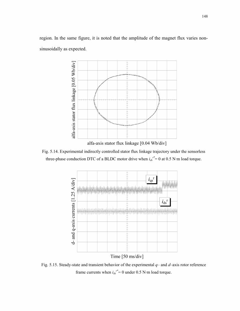
148
region. In the same figure, it is noted that the amplitude of the magnet flux varies non-
sinusoidally as expected.
alfa
-axi
s sta
tor f
lux
linka
ge [0
.05
Wb/
div]
alfa-axis stator flux linkage [0.04 Wb/div] Fig. 5.14. Experimental indirectly controlled stator flux linkage trajectory under the sensorless
three-phase conduction DTC of a BLDC motor drive when idsr*= 0 at 0.5 N·m load torque.
Time [50 ms/div]
d- a
nd q
-axi
s cur
rent
s [1.
25 A
/div
]
iqsr
idsr
Fig. 5.15. Steady-state and transient behavior of the experimental q– and d–axis rotor reference
frame currents when idsr*= 0 under 0.5 N·m load torque.

149
q– and d–axis currents used in (5.32) are illustrated in Fig. 5.15 from top to
bottom, respectively under 0.5 N·m load torque. At 0.425 second the torque reference is
increased and the change in the q–axis frame current is noted in Fig. 5.15. In the same
figure, q–axis current fluctuates around a dc offset to obtain smooth electromagnetic
torque. It is seen in Fig. 5.15 that the d–axis current oscillates around the desired zero
reference value which means that the stator flux amplitude equals the magnet flux.
Actual and estimated electrical rotor positions are shown in Fig. 5.16 from top to
bottom, respectively. Experimental estimated electrical rotor position is capable of
tracking the actual position quite well. Because the estimation algorithm depends on the
winding inductance as well as resistance, their variations should be considered.
However, this is left as a future research study.
-7
0
7-7
0
7
Est.
elec
. pos
(r
ad)
Act
. ele
c. p
os
(rad
)
Time [50 ms/div]
Fig. 5.16. Steady-state and transient behavior of the actual and estimated electrical rotor
positions from top to bottom under 0.5 N·m load torque.
26143 data for each line-to-line back-EMF (eba and eca) is obtained using an
oscilloscope. Then, it is converted to back-EMF constant (kd and kq) and down sampled
to 252 data in Matlab/Simulink for real-time DSP implementation. Moreover, to obtain a

150
much realistic result linear interpolation technique is performed on the 252 data in the
DSP implementation.
5.6. Conclusion
This study has successfully demonstrated application of the proposed position
sensorless three-phase conduction direct torque control (DTC) scheme for BLDC motor
drives. It is shown that the BLDC motor could also operate in the field-weakening region
by properly selecting the d–axis current reference in the proposed DTC scheme. First,
practically available actual two line-to-line back-EMF constants (kba and kca) versus
electrical rotor position are obtained using generator test and converted to the dq frame
equivalents using the new Line-to-Line Park Transformation in which only two input
variables are required. Then, they are used in the torque estimation algorithm. Electrical
rotor position required in the torque estimation is obtained using winding inductance,
stationary reference frame currents and stator flux linkages.
Since the actual back-EMF waveforms are used in the torque estimation, low-
frequency torque oscillations can be reduced convincingly compared to the one with the
ideal-trapezoidal waveforms having 120 electrical degree flat top. A look-up table for
the three-phase voltage vector selection is designed similar to a DTC of PMSM drive to
provide fast torque and flux control. Because the actual rotor flux linkage is not
sinusoidal, stator flux control with constant reference is not viable anymore. Therefore,
indirect stator flux control is performed by controlling the flux related d–axis current
using bang-bang (hysteresis) control which provides acceptable control of time-varying
signals (reference and/or feedback) quite well. Since the proposed DTC scheme does not

151
involve any PWM strategies, PI controllers as well as inverse Park and Clarke
Transformations to drive the motor, much simpler overall control is achieved.

152
CHAPTER VI
SUMMARY AND FUTURE WORK
This work presented the direct torque control (DTC) techniques, implemented in
four- and six-switch inverter, for brushless dc (BLDC) motors with non-sinusoidal back-
EMF using two and three-phase conduction modes.
In Chapter II, the proposed two-phase conduction mode for DTC of BLDC
motors is introduced as opposed to the conventional three-phase conduction DTC of
PMSM drives in the constant torque region. Much faster torque response is achieved
compared to conventional PWM current and especially voltage control techniques. It is
also shown that in the constant torque region under the two-phase conduction DTC
scheme, the amplitude of the stator flux linkage cannot easily be controlled due to the
sharp changes and the curved shape of the flux vector between two consecutive
commutation points in the stator flux linkage locus. Furthermore, to eliminate the low-
frequency torque oscillations caused by the non-ideal trapezoidal shape of the actual
back-EMF waveform of the BLDC motor, pre-stored back-EMF constants in αβ–axes
versus electrical rotor position look-up tables are designed and used in the torque
estimation algorithm.
In Chapter III, the avarege current controlled boost power factor correction
(PFC) method is applied to the previously discussed proposed DTC of BLDC motor
drive in the constant torque region. The duty cycle of the boost converter is determined

153
by a control algorithm. This control algorithm is based on the input voltage, output
voltage which is the dc-link of the BLDC motor drive, and the inductor current using the
average current control method with input voltage feed-forward compensation during
each sampling period of the drive system. The test results verify that the proposed PFC
for DTC of BLDC motor drive improves the power factor from 0.77 to about 0.9997
irrespective of the load.
In Chapter IV, the DTC technique for BLDC motor using four-switch inverter in
the constant torque region is studied. The results show that the direct torque controlled
four-switch three-phase BLDC motor drive could be a good alternative to the
conventional six-switch counterpart with respect to low cost and high performance.
Since the flux control and PWM generation are removed in the above two methods,
fewer algorithms are required for the proposed control schemes.
Finally, the position sensorless direct torque and indirect flux control (DTIFC) of
BLDC motor with non-sinusoidal (non-ideal trapezoidal) back-EMF has been
extensively investigated using three-phase conduction scheme with six-switch inverter.
In the literature, several methods have been proposed to eliminate the low-frequency
torque pulsations for BLDC motor drives such as Fourier series analysis of current
waveforms and either iterative or least-mean-square minimization techniques. Most
methods do not consider the stator flux linkage control, therefore possible high-speed
operations are not feasible. In this work, a novel and simple approach to achieve a low-
frequency torque ripple-free direct torque control with maximum efficiency based on dq
reference frame similar to permanent magnet synchronous motor (PMSM) drives is

154
presented. The electrical rotor position is estimated using winding inductance, and the
stationary reference frame stator flux linkages and currents. The proposed sensorless
DTC method controls the torque directly and stator flux amplitude indirectly using d–
axis current. Since stator flux is controllable, flux-weakening operation is possible.
Moreover, this method also permits to regulate the varying references. Simple voltage
vector selection look-up table is designed to obtain fast torque and flux control.
Furthermore, to eliminate the low-frequency torque oscillations, two actual and easily
available line-to-line back-EMF constants (kba and kca) according to electrical rotor
position are obtained offline and converted to the dq frame equivalents using the new
Line-to-Line Park Transformation. Then, they are set up in the look-up table for torque
estimation.
Theoretical concepts are developed, and the validity and effectiveness of the
proposed three-phase conduction DTC of BLDC motor drive scheme discussed above
are verified through the simulations and experimental results.
Possible future research of the previously explained DTC of BLDC motor drive
techniques will be discussed in the following:
In Chapter II and IV, a position estimation technique can be used both in six- and
four-switch DTC of BLDC motor drive instead of an expensive and bulky position
encoder for a cost-effective system. When back-EMF estimation method is selected as a
position sensorless technique, parameter variations should also be considered especially
in low speed region. Because at very low speeds the back-EMF information is very weak
and quite comparable with the supply voltage, any variation in resistance in conjunction

155
with current and voltage sensing errors (offset errors causing a drift in integration) will
degrade the flux estimation and the overall system may become unstable.
In Chapter III, the power factor control technique can be coupled with the
proposed two-phase conduction DTC of BLDC motor drive to improve the current and
torque performance at high dc-link voltage conditions while keeping the dc-link voltage
fluctuations at minimum and power factor at maximum level.
In Chapter IV, the control of phase torque (Tea and Teb) can be replaced with the
line-to-line torque control which eliminates the need for phase back-EMFs, therefore
easily available line-to-line back-EMFs can be used in the torque control scheme.
In Chapter V, resistance, inductance and even back-EMF constant variations can
be updated online for adaptive control to improve the efficiency and controllability of
the overall system in any conditions. Back-EMF used in the torque estimation algorithm
can be obtained in real-time instead of the offline look-up table method. Accuracy of the
real-time back-EMF information which is used in the torque equation can be analyzed
and compared with the look-up table method. Results of the overall control when torque
is estimated with online back-EMF and with look-up table can be compared under low
speed and saturation conditions. Effects of the back-EMF constant variations can also be
studied in both cases.
When the motor speed is above the rated (base) speed, the motor torque
decreases very quickly since the back-EMF rapidly approaches the dc-link voltage if the
small switch voltage drops are ignored. Eventually, the current (torque) regulators
saturate, losing the ability to force the commanded current into the motor phase. In order

156
to solve this problem, the flux-weakening technique can be developed for the proposed
DTC of BLDC motor drive in which the properly selected negative d–axis current
should be applied to weaken the field produced by the permanent magnet rotor
considering the voltage and current limitations of the BLDC machine.
Moreover, SVPWM technique can be combined with the proposed sensorless
direct torque and indirect flux control (DTIFC) method to reduce the current and torque
ripples while keeping the robustness in the torque control. Also, instead of six-switch
inverter four-switch one as in Chapter IV can be used to minimize the cost of the overall
system.
Because the possible mechanical/magnetic discrepancy of the rotor magnets over
one mechanical rotation using actual back-EMF data containing one complete
mechanical cycle will be more effective to eliminate the low-frequency torque ripples in
the proposed DTC of BLDC motor drives. If the pole number of the machine is high
more data is required to obtain the back-EMF in one mechanical cycle. Therefore, the
memory requirement will be increased.

157
REFERENCES
[1] K. Hasse, “Drehzahlgelverfahren für schnelle umkehrantriebe mit stromrichtergespeisten asynchron-kurzschlusslaufer-motoren,” Reglungstechnik, vol. 20, pp. 60–66, 1972.
[2] S. P. Waikar, “A low-cost low-loss brushless permanent magnet motor drive.” Ph.D. dissertation, Texas A&M University, College Station, TX, 2001.
[3] J. Luukko, “Direct torque control of permanent magnet synchronous machines - analysis and implementation.” Ph.D. dissertation, Lappeenranta University of Technology, Lappeenranta , Finland, 2000.
[4] I. Takahashi and T. Noguchi, “A new quick-response and high efficiency control strategy of an induction machine,” IEEE Trans. Ind. Appl., vol. IA–22, pp. 820–827, Sep./Oct. 1986.
[5] U. Baader, M. Depenbrock, and G. Gierse, “Direct self control (DSC) of inverter-fed-induction machine—A basis for speed control without speed measurement,” IEEE Trans. Ind. Appl., vol. 28, pp. 581–588, May/Jun. 1992.
[6] M. Depenbrock, “Direct self control of inverter-fed induction machines,” IEEE Trans. Power Electron., vol. 3, pp. 420–429, Oct. 1988.
[7] M. Depenbrock, “Direct self-control of the flux and rotary moment of a rotary-field machine,” U.S. Patent 4 678 248, Jul. 7, 1987.
[8] P. Vas, Vector Control of AC Machines. London, U.K.: Oxford Univ. Press, 1990.
[9] C. French and P. Acarnley, “Direct torque control of permanent magnet drives,” IEEE Trans. Ind. Appl., vol. IA–32, pp. 1080–1088, Sep./Oct. 1996.
[10] L. Zhong, M. F. Rahman, W. Y. Hu, and K. W. Lim, “Analysis of direct torque control in permanent magnet synchronous motor drives,” IEEE Trans. Power Electron., vol. 12, pp. 528–536, May 1997.
[11] I. Takahashi and T. Noguchi, “Take a look back upon the past decade of direct torque control,” in Proc. IEEE-IECON Annu. Meeting, vol. 2, 1997, pp. 546–551.
[12] D. Casadei, G. Serra, and A. Tani, “Implementation of a direct torque control algorithm for induction motors based on discrete space vector modulation,” IEEE Trans. Power Electron., vol. 15, pp. 769–777, Jul. 2000.

158
[13] C. G. Mei, S. K. Panda, J. X. Xu, and K. W. Lim, “Direct torque control of induction motor-variable switching sectors,” in Proc. IEEE-PEDS Annu. Meeting, Hong Kong, Jul. 1999, pp. 80–85.
[14] A. Tripathi, A. M. Khambadkone, and S. K. Panda, “Space-vector based, constant frequency, direct torque control and dead beat stator flux control of ac machines,” in Proc. IEEE-IECON Annu. Meeting, Nov. 2001, pp. 1219–1224.
[15] C. Lascu, I. Boldea, and F. Blaabjerg, “A modified direct torque control for induction motor sensorless drive,” IEEE Trans. Ind. Appl., vol. 36, pp. 122–130, Jan./Feb. 2000.
[16] D. Swierczynski, M. Kazmierkowski, and F. Blaabjerg, “DSP based direct torque control of permanent magnet synchronous motor (PMSM) using space vector modulation (DTC-SVM),” in Proc. IEEE-ISIE Annu. Meeting, vol. 3, May 2002, pp. 723–727.
[17] L. Tang , L. Zhong, M. F. Rahman, and Y. Hu “A novel direct torque control for interior permanent-magnet synchronous machine drive with low ripple in torque and flux-a speed-sensorless approach,” in Proc. IEEE Trans. Ind. Appl., vol. 39, pp. 1748–1756, Nov./Dec. 2003.
[18] C. Martins, X. Roboam, T. A. Meynard, and A. S. Caryalho, “Switching frequency imposition and ripple reduction in DTC drives by using a multilevel converter,” IEEE Trans. Power Electron., vol. 17, pp. 286–297, Mar. 2002.
[19] Y. A. Chapuis, D. Roye, and J. Davoine, “Principles and implementation of direct torque control by stator flux orientation of an induction motor,” in Conf. Rec. IEEE-IAS Annu. Meeting, vol. 1, 1995, pp. 185–191.
[20] B. K. B. And and N. R. Patel, “A programmable cascaded low-pass filter-based flux synthesis for a stator flux-oriented vector-controlled induction motor drive,” IEEE Trans. Ind. Electron., vol. 44, pp. 140–143, Feb. 1997.
[21] M. R. Zolghadri and D. Roye, “A fully digital sensorless direct torque control system for synchronous machine,” Elect. Mach. Power Syst., vol. 26, pp. 709–721, 1998.
[22] P. Vas. Sensorless Vector and Direct Torque Control. London, U.K.: Oxford Univ. Press, 1998.
[23] M. F. Rahman, Md. E. Haque, L. Tang, and L. Zhong, “Problems associated with the direct torque control of an interior permanent-magnet synchronous motor drive and their remedies,” IEEE Trans. Ind. Electron., vol. 51, pp. 799–809, Aug. 2004.

159
[24] S. Mir, M. E. Elbuluk, and D. S. Zinger, “PI and fuzzy estimators for tuning the stator resistance in direct torque control of induction machines,” IEEE Trans. Power Electron., vol. 13, pp. 279–287, Mar. 1998.
[25] L. Zhong, M. F. Rahman, K. W. Lim, Y. Hu, and Y. Xu, “A fuzzy observer for induction motor stator resistance for application in direct torque control,” in Proc. IEEE-PEDS Annu. Meeting, 1997, pp. 91–96.
[26] B. S. Lee and R. Krishnan, “Adaptive stator resistance compensator for high performance direct torque controlled induction motor drive,” in Conf. Rec. IEEE-IAS Annu. Meeting, St. Louis, MO, 1998, pp. 423–423.
[27] M. E. Haque and M. F. Rahman, “Influence of stator resistance variation on direct torque controlled interior permanent magnet synchronous motor drive performance and its compensation,” in Proc. IEEE-IAS Annu. Meeting, 2001, pp. 2563–2569.
[28] R. Dhaouadi, N. Mohan, and L. Norum, “Design and implementation of an extended Kalman filter for the state estimation of a permanent magnet synchronous motor,” IEEE Trans. Power Electron., vol. 6, no. 3, pp. 491–497, 1991.
[29] M. Schroedl, “Sensorless control of ac machines at low speed and standstill based on the “INFORM” method,” in Proc. IEEE-IAS Annu. Meeting, San Diego, CA, Oct. 6–10, 1996, pp. 270–277.
[30] M. Schroedl, “Sensorless control of permanent magnet synchronous motors,” Elect. Mach. Power Syst., vol. 22, no. 2, pp. 173–185, Mar./Apr. 1994.
[31] R. B. Sepe and J. H. Lang, “Real-Time observer-based (adaptive) control of a permanent-magnet synchronous motor without mechanical sensors,” IEEE Trans. Ind. Appl., vol. 28, pp. 1345–1352, Nov./Dec. 1992.
[32] A. B. Kulkarni and M. Ehsani, “A novel position sensor elimination technique for the interior permanent magnet synchronous motor drive,” IEEE Trans. Ind. Appl., vol. 28, pp. 144–150, Jan./Feb. 1992.
[33] S. Ogasawara and H. Akagi, “An approach to real time position estimation at zero and low speed for a PM motor based on saliency,” in Proc. IEEE-IAS Annu. Meeting, San Diego, CA, Oct. 6–10, 1996, pp. 29–35.
[34] S. Ostlund and M. Brokemper, “Sensorless rotor-position detection from zero to rated speed for an integrated PM synchronous motor drive,” IEEE Trans. Ind. Appl., vol. 32, pp. 1158–1165, Sep./Oct. 1996.

160
[35] P. B. Schmidt, M. L. Gasperi, G. Ray, and A. H. Wijenayake, “Initial rotor angle detection of a nonsalient pole permanent magnet synchronous machine,” in Proc. IEEE-IAS Annu. Meeting, New Orleans, LA, Oct. 5–9, 1997, pp. 549–463.
[36] T. Noguchi, K. Yamada, S. Kondo, and I. Takahashi, “Initial rotor position estimation method of sensorless PM motor with no sensitivity to armature resistance,” IEEE Trans. Ind. Electron., vol. 45, pp. 118–125, Feb. 1998.
[37] M. W. Degner and R. D. Lorenz, “Using multiple saliencies for the estimation of flux, position, and velocity in ac machines,” in Proc. IEEE-IAS Annu. Meeting, New Orleans, LA, Oct. 5–9, 1997, pp. 760–767.
[38] M. J. Corley and R. D. Lorenz, “Rotor position and velocity estimation for a salient-pole permanent magnet synchronous machine at standstill and high speeds,” IEEE Trans. Ind. Appl., vol. 34, pp. 784–789, Jul./Aug. 1998.
[39] A. Consoli, G. Scarcella, and A. Testa, “Sensorless control of ac motors at zero speed,” in Proc. IEEE-ISIE Annu. Meeting, vol. 1, Bled, Slovenia, Jul. 1999, pp. 373–379.
[40] B. K. Bose. Modern Power Electronics and AC Drives. Upper Saddle River, NJ: Prentice Hall PTR., 2002.
[41] L. Hao, H. A. Toliyat, “BLDC motor full-speed operation using hybrid sliding mode observer,” in Proc. IEEE-APEC Annu. Meeting, Miami, FL, Feb. 9-13, 2003, vol. 1, pp. 286-293.
[42] P. Pillay and R. Krishnan, “Application characteristics of permanent magnet synchronous and brushless dc motors for servo drives,” IEEE Trans. Ind. Appl., vol. 27, no. 5, pp. 986–996, Sep./Oct. 1991.
[43] P. J. Sung,W. P. Han, L. H. Man, and F. Harashima, “A new approach for minimum-torque-ripple maximum-efficiency control of BLDC motor,” IEEE Trans. Ind. Electron., vol. 47, no. 1, pp. 109–114, Feb. 2000.
[44] C. French and P. Acarnley, “Direct torque control of permanent magnet drives,” IEEE Trans. Ind. Appl., vol. 32, no. 5, pp. 1080–1088, Sep./Oct. 1996.
[45] S. J. Kang and S. K. Sul, “Direct torque control of brushless dc motor with nonideal trapezoidal back-EMF,” IEEE Trans. Power Electron., vol. 10, no. 6, pp. 796–802, Nov. 1995

161
[46] S. K. Chung, H. S. Kim, C. G. Kim, and M. J. Youn, “A new instantaneous torque control of PM synchronous motor for high-performance direct-drive applications,” IEEE Trans. Power Electron., vol. 13, no. 3, pp. 388–400, May 1998.
[47] T. S. Low, K. J. Tseng, T. H. Lee, K. W. Lim, and K. S. Lock, “Strategy for the instantaneous torque control of permanent-magnet brushless dc drives,” in Proc. IEE Elect. Power Appl., vol. 137, no. 6, pp. 355–363, Nov. 1990.
[48] T. S. Low, T. H. Lee, K. J. Tseng, and K. S. Lock, “Servo performance of a BLDC drive with instantaneous torque control,” IEEE Trans. Ind. Appl., vol. 28, no. 2, pp. 455–462, Mar./Apr. 1992.
[49] K. Y. Cho, J. D. Bae, S. K. Chung, and M. J. Youn, “Torque harmonics minimization in permanent magnet synchronous motor with back-EMF estimation,” in Proc IEE Elec. Power Appl., vol. 141, no. 6, pp. 323–330, 1994.
[50] D. Grenier, L. A. Dessaint, O. Akhrif, J. P. Louis, “A park-like transformation for the study and the control of a nonsinusoidal brushless dc motor,” in Proc. IEEE-IECON Annu. Meeting, Orlando, FL, Nov. 6-10, 1995, vol. 2, pp. 836–843.
[51] F. Bodin, S. Siala, “New reference frame for brushless dc motor drive,” in Proc. IEE-PEVD Annu. Meeting, London, UK, Sep. 21-23, 1998, pp. 554-559.
[52] D. Grenier, S. Yala, O. Akhrif, L. A. Dessaint, “Direct torque control of pm ac motor with non-sinusoidal flux distribution using state-feedback linearization techniques,” in Proc. IEEE-IECON Annu. Meeting, Aachen, Germany, Aug. 31-Sep. 4, 1998, vol. 3, pp. 1515–1520.
[53] I. Takahashi and T. Noguchi, “A new quick-response and high-efficiency control strategies of an induction motor,” IEEE Trans. Ind. Appl., vol. 22, no. 5, pp. 820–827, Sep./Oct. 1986.
[54] M. Depenbrock, “Direct self-control of inverter-fed induction machine,” IEEE Trans. Power Electron., vol. 3, no. 4, pp. 420–429, Oct. 1988.
[55] L. Zhong, M. F. Rahman, W. Y. Hu, and K. W. Lim, “Analysis of direct torque control in permanent magnet synchronous motor drives,” IEEE Trans. Power Electron., vol. 12, no. 3, pp. 528–536, May 1997.
[56] Y. Liu, Z. Q. Zhu, and D. Howe, “Direct torque control of brushless dc drives with reduced torque ripple,” IEEE Trans. Ind. Appl., vol. 41, no. 2, pp. 599–608, Mar./Apr. 2005.

162
[57] W. S. H. Wong, D. Holliday, “Constant inverter switching frequency direct torque control,” in Proc. IEE-PEMD Annu. Meeting, Bath, UK, Jun. 4-7, 2002, pp. 104–109.
[58] M. Ehsani, R. C. Becerra, “High-speed torque control of brushless permanent magnet motors,” IEEE Trans. Ind. Electron., vol. 35, no. 3, pp. 402–406, Aug. 1988.
[59] P. C. Todd, “UC3854 controlled power factor correction circuit design,” U-134, Unitrode Application Note, pp. 3-269–3-288.
[60] R. Redl and B. P. Erisman, “Reducing distortion in peak-current-controlled boost power-factor correctors,” in Proc. IEEE-APEC Annu. Meeting, Orlando, FL, Feb. 13-17, 1994, vol. 2, pp. 576–583.
[61] J. Spangler and A. Behera, “A comparison between hysteretic and fixed frequency boost converters used for power factor correction,” in Proc. IEEE-APEC Annu. Meeting, San Diego, CA, Mar. 7-11, 1993, pp. 281–286.
[62] R. Zane and D. Maksimovic, “Nonlinear-carrier control for high-power factor rectifiers based on up-down switching converters,” IEEE Trans. Power Electron., vol. 13, no. 2, pp. 213–221, Mar. 1998.
[63] W. Zhang, G. Feng, Y.-F. Liu, and B. Wu, “A digital power factor correction (PFC) control strategy optimized for DSP,” IEEE Trans. Power Electron., vol. 19, no. 6, pp. 1474–1485, Nov. 2004.
[64] M. Fu and Q. Chen, “A DSP based controller for power factor correction in a rectifier circuit,” in Proc. IEEE-APEC Annu. Meeting, Anaheim, CA, Mar. 4-8, 2001, pp. 144–149.
[65] S. Buso et al., “Simple digital control improving dynamic performance of power factor pre-regulators,” IEEE Trans. Power Electron., vol. 13, no. 5, pp. 814–823, Sep. 1998.
[66] J. Zhou et al., “Novel sampling algorithm for DSP controlled 2 kW PFC converter,” IEEE Trans. Power Electron., vol. 16, no. 2, pp. 217–222, Mar. 2001.
[67] S. Choudhury, “Average current mode controlled power factor correction converter using TMS320LF2407A,” Texas Instruments Application Note SPRA902A, Jul. 2005, pp. 1–14.

163
[68] H.W. Van Der Broeck and J. D. Van Wyk, “A comparative investigation of a tree-phase induction machine drive with a component minimized voltage-fed inverter under different control options,” IEEE Trans. Ind. Appl., vol. 20, no. 2, pp. 309–320, Mar./Apr. 1984.
[69] B-K. Lee, T-K. Kim and M. Ehsani, “On the feasibility of four-switch three-phase BLDC motor drives for low cost commercial applications: topology and control,” IEEE Trans. Power. Electron., vol. 18, no. 1, pp. 164–172, Jan. 2003.
[70] S-H. Park, T-S. Kim, S-C. Ahn, D-S. Hyun, “A simple current control algorithm for torque ripple reduction of brushless dc motor using four-switch three-phase inverter,” in Proc. IEEE-PESC Annu. Meeting, Jun. 15-19, 2003, vol. 2, pp. 574–579.
[71] J-H. Lee, S-C. Ahn, D-S. Hyun, “A BLDCM drive with trapezoidal back EMF using four-switch three phase inverter,” in Proc. IEEE-IAS Annu. Meeting, Oct. 8-12, 2000, vol. 3, pp. 1705–1709.
[72] S. B. Ozturk and H. A. Toliyat, “Direct torque control of brushless dc motor with non-sinusoidal back-EMF,” in Proc. IEEE-IEMDC Biennial Meeting, Antalya, Turkey, May 3-5, 2007.
[73] H. R. Bolton and R. A. Ashen, “Influence of motor design and feedcurrent waveform on torque ripple in brushless dc drives,” in Proc. IEE Elect. Power Appl., vol. 131, no. 3, pp. 82–90, 1984.
[74] B. H. Ng, M. F. Rahman, and T. S. Low, “An investigation into the effects of machine parameters on torque pulsation in a brushless dc drive,” in Proc. IEEE- IECON, 1988, pp. 749–754.
[75] H. L. Huy, R. Perret, and R. Feuillet, “Minimization of torque ripple in brushless dc motor drives,” IEEE Trans. Ind. Appl., vol. 22, no. 4, pp. 748–755, 1986.
[76] F. Piriou, A. Razek, R. Perret, and H. L. Huy, “Torque characteristics of brushless dc motors with imposed current waveform,” in Proc. IEEE-IAS Annu. Meeting, 1986, pp. 176–181.
[77] D. Hanselman, “Minimum torque ripple, maximum efficiency excitation of brushless permanent magnet motors,” IEEE Trans. Ind. Electron., vol. 41, no. 3, pp. 292–300, 1994.
[78] N. Matsui, T. Makino, and H. Satoh, “Auto-compensation of torque ripple of DD motor by torque observer,” IEEE Trans. Ind. Appl., vol. 29, no. 1, pp. 187–194, 1993.

164
[79] T. Kim, H-W Lee, L. Parsa, and M. Ehsani, “Optimal power and torque control of a brushless dc (BLDC) motor/generator drive in electric and hybrid electric vehicles,” in Proc. IEEE-IAS Annu. Meeting, 8-12 Oct. 2006, vol. 3, pp. 1276–1281.
[80] P. L. Chapman, S.D. Sudhoff, and C.A. Whitcomb, “Multiple reference frame analysis of non-sinusoidal brushless dc drives,” IEEE Trans. Eng. Convers. vol. 143, pp. 440 –446. Sep. 1999.
[81] R. H. Park, “Two-reaction theory of synchronous machines, generalized method of analysis - Part I” AIEE Trans., vol. 48, pp. 716–730, Jul. 1929.
[82] C. M. Ong. Dynamic Simulation of Electric Machinery Using MATLAB / SIMULINK. Upper Saddle River, NJ: Prentice Hall PTR, 1998.
[83] J. Hu, B. Wu, “New integration algorithms for estimating motor flux over a wide speed range,” IEEE Trans. Power Electrons., vol. 13, pp. 969–977, Sep. 1998.

165
APPENDIX A
kca(θe)kbc(θe) L
ine-
to-li
ne b
ack-
EM
F co
nsta
nts
[0.1
Wb/
div]
Electrical Rotor Position [pi/5 rad/div]
0
kab(θe)
(a)
kβ(θe)
alfa
&be
ta-a
xes
back
-EM
F co
nsta
nts
[0.0
5 W
b/di
v]
Electrical Rotor Position [pi/5 rad/div]
0
kα(θe)
(b)
Fig. A.1. (a) Actual line-to-line back-EMF constants (kab(θe), kbc(θe), and kca(θe)) and (b)
stationary reference frame back-EMF constants (kα(θe) and kβ(θe)).

166
SPECIFICATIONS AND PARAMETERS OF THE BLDC MOTOR
Symbol Quantity Value P Number of poles 4
VLL Maximum line-to-line voltage (Vrms) 115 Ipk Maximum peak current (A) 24
Irated Rated current (A) 5.6 Trated Rated torque (N·m) 1.28352
Ls Winding inductance (mH) 1.4 M Mutual inductance (mH) 0.3125 Rs Winding resistance (ohm) 0.315 λf Rotor magnetic flux linkage (Wb) 0.1146 λfmax Maximum rotor magnetic flux linkage (Wb) 0.1304

167
APPENDIX B
The electromagnetic torque equation for a BLDC motor consisting of ba–ca
reference frame variables can be derived as follows:
The line-to-line components constituting the electromagnetic torque equation can
be obtained by using Clarke Transformation which is given by
1 112 2 23 3 30
2 2
a
b
c
XX
XX
X
α
β
⎛ ⎞⎛ ⎞− −⎜ ⎟⎛ ⎞ ⎜ ⎟⎜ ⎟=⎜ ⎟ ⎜ ⎟⎜ ⎟⎝ ⎠ ⎜ ⎟−⎜ ⎟⎝ ⎠⎝ ⎠
(B.1)
where Xα and Xβ are the stationary reference frame components, and Xa, Xb, and Xc are
the abc frame components. X in (B.1) represents currents and/or rotor flux linkages in
the electromagnetic torque equation.
If Xα and Xβ are expanded and algebraically manipulated, the line-to-line
representations of Xα and Xβ in ba–ca reference frame are attained respectively as
23 3
3
a b c a b a c
ba ca
X X X X X X XX
X X
α− − − + −
= =
− −=
(B.2)
and
( ) ( )
( )
3 33 33
3
b c b a a c
ba ca
X X X X X X X
X X
β = − = − + −
= −
(B.3)

168
where Xba = Xb − Xa and Xca = Xc − Xa.
Using the results obtained in (B.2) and (B.3), Xα and Xβ can be rewritten in matrix
form as
1 13 33 3
3 3
ba
ca
X XX X
α
β
⎛ ⎞− −⎜ ⎟⎛ ⎞ ⎛ ⎞⎜ ⎟=⎜ ⎟ ⎜ ⎟⎜ ⎟⎝ ⎠⎝ ⎠ −⎜ ⎟⎝ ⎠
(B.4)
If the matrix in (B.4) is used in (2.16), the electromagnetic torque equation in
terms of ba–ca frame line-to-line components can be expressed as follows:
( )
( )
1/ 3 1/ 33 ( 1/ 3 1/ 3 )2 2
3 / 3 3 / 3( 3 / 3 3 / 3 )
rba rcaem ba ca
e
rba rcaba ca
e
dPT i id
di i
d
ϕ ϕθ
ϕ ϕ
θ
⎧ − −= − − +⎨
⎩⎫− ⎪− ⎬⎪⎭
(B.5)
After algebraically simplifying (B.5), the electromagnetic torque equation is
obtained as
2 2
6rba rca rca rba
em ba cae e e e
d d d dPT i i
d d d d
ϕ ϕ ϕ ϕ
θ θ θ θ= − + −
⎡ ⎤⎛ ⎞ ⎛ ⎞⎟ ⎟⎜ ⎜⎢ ⎥⎟ ⎟⎜ ⎜⎟ ⎟⎢ ⎥⎜ ⎜⎟ ⎟⎜ ⎜⎝ ⎠ ⎝ ⎠⎢ ⎥⎣ ⎦ (B.6)
where P is the pole number, dφrba/dθ e and dφrca/dθ e are the derivatives of the ba– and
ca–axis rotor flux linkages over electrical rotor position, iba = ib − ia, and ica = ic − ia.
If (B.6) is rewritten in terms of line-to-line back-EMFs the torque equation can
be given in the following:
2 26
ba ca ca baem ba ca
e e
e e e ePT i iω ω
⎡ ⎤⎛ ⎞ ⎛ ⎞− −⎟ ⎟⎜ ⎜⎢ ⎥⎟ ⎟= +⎜ ⎜⎟ ⎟⎢ ⎥⎜ ⎜⎟ ⎟⎜ ⎜⎝ ⎠ ⎝ ⎠⎢ ⎥⎣ ⎦ (B.7)

169
where eba = eb − ea, eca = ec − ea, and ωe is the electrical rotor speed. As a result, two
line-to-line back-EMFs (eba, eca) and currents (iba, ica) are enough to estimate the
electromagnetic torque. The problematic electrical rotor speed ωe in (B.7) can be
removed if the two electrical rotor position dependant line-to-line back-EMF constants
are used in the electromagnetic torque equation which is given by
( ) ( )2 ( ) ( ) 2 ( ) ( )
6em ba e ca e ba ca e ba e caPT k k i k k iθ θ θ θ⎡ ⎤= − + −⎣ ⎦ (B.8)
Another torque equation similar to (2.16) using line-to-line model in ab–bc–ca
reference frame can be obtained as
2 3ab ab bc bc ca ca
eme
e i e i e iPT
ω
+ +=
⎛ ⎞⎟⎜ ⎟⎜ ⎟⎜ ⎟⎜⎝ ⎠ (B.9)
where ebc = eb − ec, and ibc = ib − ic.
Even though (B.9) has fewer components compared to (B.8), there are additional
line-to-line back-EMF and current components in bc–axis. Equation (B.9) can further be
simplified by removing the electrical rotor speed ωe in the denominator allowing zero
and near zero speed torque estimation possible as follows:
( )) ) )( ( (
6em ab ab bc bc ca cae e eP
T k i k i k iθ θ θ= + + (B.10)
As a result, the electromagnetic torque equations given in (B.8) and (B.10) avoid
the use of the line-to-neutral back-EMF components. They only require line-to-line
back-EMFs which can be measured directly even if the motor neutral connection is not
accessible.

170
APPENDIX C
Switching functions of the six non-zero voltage space vectors V1, V2, ..., V6 of the
six-switch DTC of BLDC motor drive, which are represented in stationary reference
frame (Vxα and Vxβ), can be derived as follows:
Six non-zero voltage space vectors which are used in six-switch DTC of BLDC
motor drive can be shown in the following form:
1 2 3 4 5 6( )xV S S S S S S (C.1)
where x is between 1 and 6, and S1, S2,…, S6 are the switch states. “1” represents on state
and “0” is off state of the corresponding switch.
αβ–axes six-switch voltage vectors (Vxα and Vxβ) can be obtained using Fig. 2.1
as follows:
1 1 13(1 0 0 0 0 1) ,2 2
dc dcV VV V Vα β⇒ = = (C.2)
2 2 2(0 0 1 0 0 1) 0,2dcVV V Vα β⇒ = = (C.3)
3 3 33(0 1 1 0 0 0) ,2 2
dc dcV VV V Vα β⇒ = − = (C.4)
4 4 43(0 1 0 0 1 0) ,2 2
dc dcV VV V Vα β⇒ = − = − (C.5)
5 5 5(0 0 0 1 1 0) 0,2dcVV V Vα β⇒ = = − (C.6)
6 6 63(1 0 0 1 0 0) ,2 2
dc dcV VV V Vα β⇒ = = − (C.7)

171
By performing some algebraic manipulations on (C.1) through (C.7), the final
switching function of αβ–axes four-switch voltage vectors (Vxα and Vxβ) can be given
respectively as
( ) ( )1 6 4 2 3 53
2x dcV V S S S S S Sα = + − +⎡ ⎤⎣ ⎦ (C.8)
( ) ( ) ( )6 1 3 2 3 5 4 5 12dc
xVV S S S S S S S S Sβ = + + − − +⎡ ⎤⎣ ⎦ (C.9)

172
APPENDIX D
Switching functions of the eight voltage space vectors V0, V1, ..., V7 of four-
switch DTC of BLDC motor drive, which are represented in stationary reference frame
(Vxα and Vxβ), can be derived as follows:
Eight voltage space vectors which are used in four-switch DTC of BLDC motor
drive can be shown in the following form:
1 2 3 4( )xV S S S S (D.1)
where x is between 0 and 7, and S1, S2,…, S4 are the switch states. “1” represents on state
and “0” is off state of the corresponding switch.
αβ–axes four-switch voltage vectors (Vxα and Vxβ) can be obtained using Fig. 4.3
as follows:
1 1 13(1 0 0 0) ,4 4
dc dcV VV V Vα β⇒ = = (D.2)
2 2 2(0 0 1 0) , 02dcVV V Vα β⇒ = = (D.3)
3 3 33(0 1 1 0) ,2 2
dc dcV VV V Vα β⇒ = − = (D.4)
4 4 43(0 1 0 0) ,4 4
dc dcV VV V Vα β⇒ = − = − (D.5)
5 5 5(0 0 0 1) , 02dcVV V Vα β⇒ = − = (D.6)
6 6 63(1 0 0 1) ,2 2
dc dcV VV V Vα β⇒ = = − (D.7)

173
0 0 03(0 1 0 1) ,
6 6dc dcV VV V Vα β⇒ = = (D.8)
7 7 73(1 0 1 0) ,
6 6dc dcV VV V Vα β⇒ = − = − (D.9)
By performing some algebraic manipulations on (D.1) through (D.9), the final
switching function of αβ–axes four-switch voltage vectors (Vxα and Vxβ) can be given
respectively as
( )1 2 2 3 1 4 2 4 1 3 2 4 1 33 2
4 3 3x dcV V S S S S S S S S S S S S S Sα⎡ ⎤= − − + + − + +⎢ ⎥⎣ ⎦
(D.10)
( )
( )
1 3 2 3 2 4 1 4 2 4 1 3
2 4 1 3
1 2 2 2 2 34
2 33
x dcV V S S S S S S S S S S S S
S S S S
β⎛= + + − − − + −⎜⎝
⎞+ − ⎟⎟
⎠
(D.11)

174
APPENDIX E
Peak value of the rotor flux linkage in stationary reference frame (φrαβ(pk)) can be
derived for a BLDC motor with an ideal trapezoidal back-EMF using easily accessible
line-to-line back-EMF waveforms as follows:
Ideal line-to-line back-EMF waveforms (eab, ebc, eca) can be illustrated in Fig. E.1
below:
bce
cae
abe
270°0° 30° 60° 90° 120° 150° 180° 210° 270°240° 360°330°300° 90°60°30° 180°150°120° 240°210°
eθ
eθ
eθ
300°
LL ek ω
Fig. E.1. Line-to-line back-EMF waveforms (eab, ebc, and eca).

175
Line-to-line back-EMF waveforms (eab, ebc, eca) shown in Fig. E.1 are converted
to αβ–axes equivalents (eα, and eβ) using Line-to-Line Clarke Transformation given by
2 1 13 3 3 3 3 3
1 103 3
ab
bc
ca
ee
ee
e
α
β
⎡ ⎤ ⎡ ⎤− −⎢ ⎥⎡ ⎤ ⎢ ⎥⎢ ⎥=⎢ ⎥ ⎢ ⎥⎢ ⎥⎣ ⎦ ⎢ ⎥− ⎣ ⎦⎢ ⎥⎣ ⎦
(E.1)
Every 60°, eα, and eβ values can be obtained using (E.1) as follows:
2At 0 0, 3 LL ee e kα β ω⇒ = = − (E.2)
1 1At 60 ,
33 LL e LL ee k e kα βω ω⇒ = = − (E.3)
1 1At 120 ,
33 LL e LL ee k e kα βω ω⇒ = = (E.4)
2At 180 0, 3 LL ee e kα β ω⇒ = = (E.5)
1 1At 240 ,
33 LL e LL ee k e kα βω ω⇒ = − = (E.6)
1 1At 300 ,
33 LL e LL ee k e kα βω ω⇒ = − = − (E.7)
2At 360 0, 3 LL ee e kα β ω⇒ = = − (E.8)
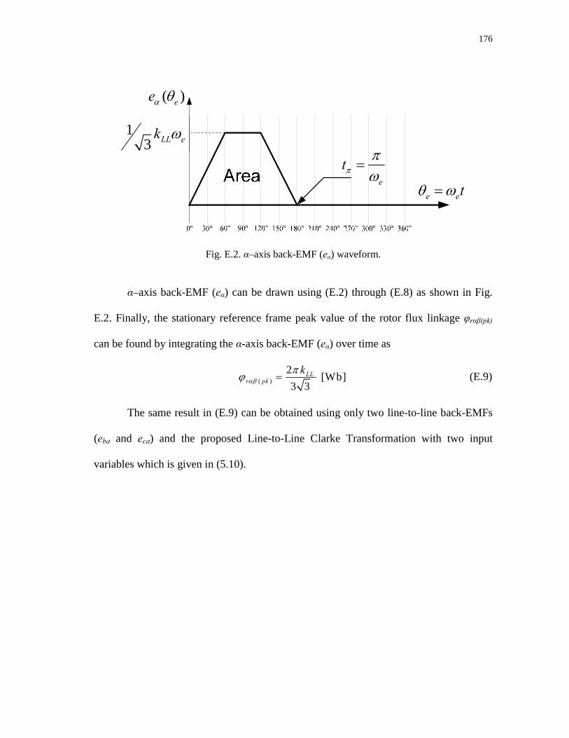
176
( )eeα θ
e etθ ω=e
tππω
=
13 LL ek ω
Fig. E.2. α–axis back-EMF (eα) waveform.
α–axis back-EMF (eα) can be drawn using (E.2) through (E.8) as shown in Fig.
E.2. Finally, the stationary reference frame peak value of the rotor flux linkage φrαβ(pk)
can be found by integrating the α-axis back-EMF (eα) over time as
( )2 [Wb]3 3
LLr pk
kαβ
πϕ = (E.9)
The same result in (E.9) can be obtained using only two line-to-line back-EMFs
(eba and eca) and the proposed Line-to-Line Clarke Transformation with two input
variables which is given in (5.10).

177
VITA
Salih Baris Ozturk received the B.S. degree (Hons.) in electrical engineering
from Istanbul Technical University, Istanbul, Turkey, in June 2000. In January 2002, he
joined the Electrical Machines and Power Electronics Laboratory research group at
Texas A&M University, College Station, TX, where he received the M.S. degree in
electrical engineering in December 2005. Prof. Hamid A. Toliyat was his advisor.
Since January 2002, Ozturk has been a graduate researcher and teaching
assistant, as well as a lecturer in the Department of Electrical and Computer Engineering
at Texas A&M University, and he has served as the EMPE lab manager since 2006. In
2004, he was also with the Whirlpool R&D Center, Benton Harbor, MI.
In May 2008, Ozturk received the Ph.D. degree in electrical engineering at Texas
A&M University under the supervision of Prof. Toliyat. His current research interests
include power factor correction for ac motor drives, fault diagnosis of electric
machinery, electric machine design, and digital signal processor-based advanced control
of ac drives, in particular sensorless and direct torque control of permanent magnet
assisted synchronous reluctance, permanent magnet synchronous and brushless dc
motors.
Ozturk also is one of the contributing authors of the book “DSP-Based
Electromagnetic Motion Control,” (Boca Raton, FL: CRC Press, 2003).
Salih Baris Ozturk is a member of the IEEE.
He may be reached in c/o
Prof. Hamid A. Toliyat Electrical Machines & Power Electronics Laboratory Department of Computer and Electrical Engineering TAMU 3128 Texas A&M University College Station, Texas 77843-3128