direct numerical simulation of bubbly flows and …lu/resume/thesis.pdfdirect numerical simulation...
TRANSCRIPT
Direct Numerical Simulation of Bubbly Flows
and Interfacial Dynamics of Phase Transitions
A Dissertation Presented
by
Tianshi Lu
to
The Graduate School in Partial Fulfillment of the Requirements for the
Degree of
Doctor of Philosophy
in
Applied Mathematics and Statistics
Stony Brook University
August 2005
Stony Brook University
The Graduate School
Tianshi Lu
We, the dissertation committee for the above candidate for the Doctor ofPhilosophy degree, hereby recommend acceptance of this dissertation.
James GlimmAdvisor
Department of Applied Mathematics and Statistics
Xiaolin LiChairman
Department of Applied Mathematics and Statistics
Yongmin ZhangMember
Department of Applied Mathematics and Statistics
Roman SamulyakOutside Member
Brookhaven National LaboratoryCenter for Scientific Computing
This dissertation is accepted by the Graduate School.
Graduate School
ii
Abstract of the Dissertation
Direct Numerical Simulation of Bubbly Flowsand Interfacial Dynamics of Phase Transitions
by
Tianshi Lu
Doctor of Philosophy
in
Applied Mathematics and Statistics
Stony Brook University
2005
We studied the propagation of acoustic and shock waves in bubbly fluids
using the Front Tracking hydrodynamic simulation code FronTier for axisym-
metric flows. We compared the simulation results with the theoretical predic-
tions and the experimental data. The method was applied to an engineering
problem on the mitigation of cavitation erosion in the container of the Spal-
lation Neutron Source liquid mercury target. The simulation of the pressure
wave in the container and the subsequent analysis on the collapse of the cavi-
tation bubbles confirmed the effectiveness of the non-condensable gas bubble
injection method on reducing cavitation damage.
Then we analyzed the interfacial dynamics of liquid-vapor phase transi-
iii
tions and the wave equations for immiscible thermal conductive fluids. The
phase transition rate is associated by the kinetic theory with the deviation of
the vapor pressure from the saturated pressure. Analytical solutions to the
linearized equations have been explored. The adiabatic and the isothermal
limits have been investigated for both the linearized and the nonlinear equa-
tions, for latter the method of travelling wave solutions has been used. The
wave structure of the solution to the problem with Riemann data has been
discussed.
We also implemented a numerical scheme for solving the Euler equations
with thermal conduction and phase transitions in the frame of front tracking.
Heat conduction has been added to the interior state update with second order
accuracy. Phase boundary propagation has been handled according to the
interfacial dynamics. A numerical technique has been introduced to account
for the thermal layer thinner than a grid cell. The scheme has been validated,
extended to multi-dimension, adapted for cylindrical and spherical symmetry,
and applied to the simulation of condensing and cavitating processes.
Key Words: bubbly flow, cavitation mitigation, phase transition, Rie-
mann problem.
iv

To my parents, wife and daughter
Table of Contents
List of Figures . . . . . . . . . . . . . . . . . . . . . . . . . . . . xvi
List of Tables . . . . . . . . . . . . . . . . . . . . . . . . . . . . xvii
Acknowledgements . . . . . . . . . . . . . . . . . . . . . . . . . xviii
1 Introduction . . . . . . . . . . . . . . . . . . . . . . . . . . . . . 1
1.1 Direct Numerical Simulation of Bubbly Flows . . . . . . . . . 1
1.2 Interfacial Dynamics of Phase Transitions . . . . . . . . . . . 4
2 Direct Numerical Simulation of Bubbly Flows . . . . . . . . 8
2.1 Theory and Experiments on Bubbly Flows . . . . . . . . . . . 8
2.1.1 Wave Equations . . . . . . . . . . . . . . . . . . . . . . 8
2.1.2 Linear Waves . . . . . . . . . . . . . . . . . . . . . . . 10
2.1.3 Shock Waves . . . . . . . . . . . . . . . . . . . . . . . 11
2.2 Numerical Method . . . . . . . . . . . . . . . . . . . . . . . . 11
2.3 Simulation Results on Bubbly Flows . . . . . . . . . . . . . . 14
2.3.1 Linear Waves . . . . . . . . . . . . . . . . . . . . . . . 15
2.3.2 Shock Waves . . . . . . . . . . . . . . . . . . . . . . . 19
vi
3 Application of Bubbly Flows to Cavitation Mitigation . . . 23
3.1 Spallation Neutron Source . . . . . . . . . . . . . . . . . . . . 24
3.2 Method of Approach . . . . . . . . . . . . . . . . . . . . . . . 26
3.3 Pressure Wave Propagation in the Container . . . . . . . . . . 28
3.4 Collapse Pressure of Cavitation Bubbles . . . . . . . . . . . . 31
3.5 Efficiency of Cavitation Damage Mitigation . . . . . . . . . . 35
4 Interfacial Dynamics of Phase Transitions . . . . . . . . . . 38
4.1 Governing Equations and Boundary Conditions . . . . . . . . 38
4.1.1 Governing Equations . . . . . . . . . . . . . . . . . . . 39
4.1.2 Boundary Conditions at Material Interface . . . . . . . 40
4.2 Alternative Forms of the Conservation Laws . . . . . . . . . . 46
4.2.1 Conservation Laws with Rotational Symmetry . . . . . 46
4.2.2 Conservation Laws on the Interface . . . . . . . . . . . 47
4.3 Analytical Solution for Immiscible Fluids: Temperature Field
Decoupled . . . . . . . . . . . . . . . . . . . . . . . . . . . . . 51
4.3.1 Analytical Solution . . . . . . . . . . . . . . . . . . . . 53
4.3.2 Example . . . . . . . . . . . . . . . . . . . . . . . . . . 57
4.3.3 Asymptotic Solution in the Adiabatic Limit . . . . . . 59
4.3.4 Asymptotic Solution in the Isothermal Limit . . . . . . 77
4.4 Analytical Solution for Phase Transitions: Temperature Field
Decoupled . . . . . . . . . . . . . . . . . . . . . . . . . . . . . 81
4.4.1 Analytical Solution . . . . . . . . . . . . . . . . . . . . 83
4.4.2 Example . . . . . . . . . . . . . . . . . . . . . . . . . . 84
4.4.3 Asymptotic Solutions . . . . . . . . . . . . . . . . . . . 84
vii
4.5 Analytical Solutions: Hyperbolic Fields Decoupled . . . . . . . 87
4.5.1 Immiscible Fluids . . . . . . . . . . . . . . . . . . . . . 87
4.5.2 Phase Transitions . . . . . . . . . . . . . . . . . . . . . 94
4.6 Full Nonlinear Equations . . . . . . . . . . . . . . . . . . . . . 97
4.6.1 Local Riemann Problem . . . . . . . . . . . . . . . . . 98
4.6.2 Travelling Wave Solutions . . . . . . . . . . . . . . . . 106
4.6.3 Adiabatic Limit . . . . . . . . . . . . . . . . . . . . . . 113
4.6.4 Wave Structure . . . . . . . . . . . . . . . . . . . . . . 121
5 Numerical Algorithm for the Simulation of Phase Transitions 123
5.1 Propagation of Phase Boundary . . . . . . . . . . . . . . . . . 124
5.1.1 Normal Propagation . . . . . . . . . . . . . . . . . . . 124
5.1.2 Thin Thermal Layer Method . . . . . . . . . . . . . . . 132
5.1.3 Tangential Propagation . . . . . . . . . . . . . . . . . . 136
5.2 Finite Difference Update of Interior States . . . . . . . . . . . 137
5.3 Validation . . . . . . . . . . . . . . . . . . . . . . . . . . . . . 141
5.3.1 Comparison with Analytical Solutions . . . . . . . . . 141
5.3.2 Thin Thermal Layer Method . . . . . . . . . . . . . . . 141
5.4 Application to One Dimensional Condensation . . . . . . . . . 149
5.4.1 Early Stage . . . . . . . . . . . . . . . . . . . . . . . . 150
5.4.2 Late Stage . . . . . . . . . . . . . . . . . . . . . . . . . 151
6 Conclusion . . . . . . . . . . . . . . . . . . . . . . . . . . . . . . 157
6.1 DNS of Bubbly Flows and Application . . . . . . . . . . . . . 157
6.2 Interfacial Dynamics of Phase Transitions . . . . . . . . . . . 158
viii
A Parameters for Stiffened Polytropic EOS . . . . . . . . . . . 160
A.1 Thermodynamic Identities . . . . . . . . . . . . . . . . . . . . 160
A.2 Liquid and Vapor EOS’s . . . . . . . . . . . . . . . . . . . . . 162
A.3 Numerical Examples . . . . . . . . . . . . . . . . . . . . . . . 164
A.3.1 Single liquid phase . . . . . . . . . . . . . . . . . . . . 164
A.3.2 Both phases near equilibrium . . . . . . . . . . . . . . 165
Bibliography . . . . . . . . . . . . . . . . . . . . . . . . . . . . . 167
ix
List of Figures
2.1 Schematic of the numerical experiments on the propagation of
linear and shock waves in bubbly fluids. . . . . . . . . . . . . . . 13
2.2 Comparison of the dispersion relation between the simulation and
the theory. R = 0.06mm, β = 0.02%. (a) is the phase velocity,
(b) is the attenuation coefficient. In both figures, the crosses are
the simulation data and the solid line is the theoretical prediction
from Eq. (2.2) with δ = 0.7. The horizontal line in figure (a) is
the sound speed in pure water. . . . . . . . . . . . . . . . . . . . 17
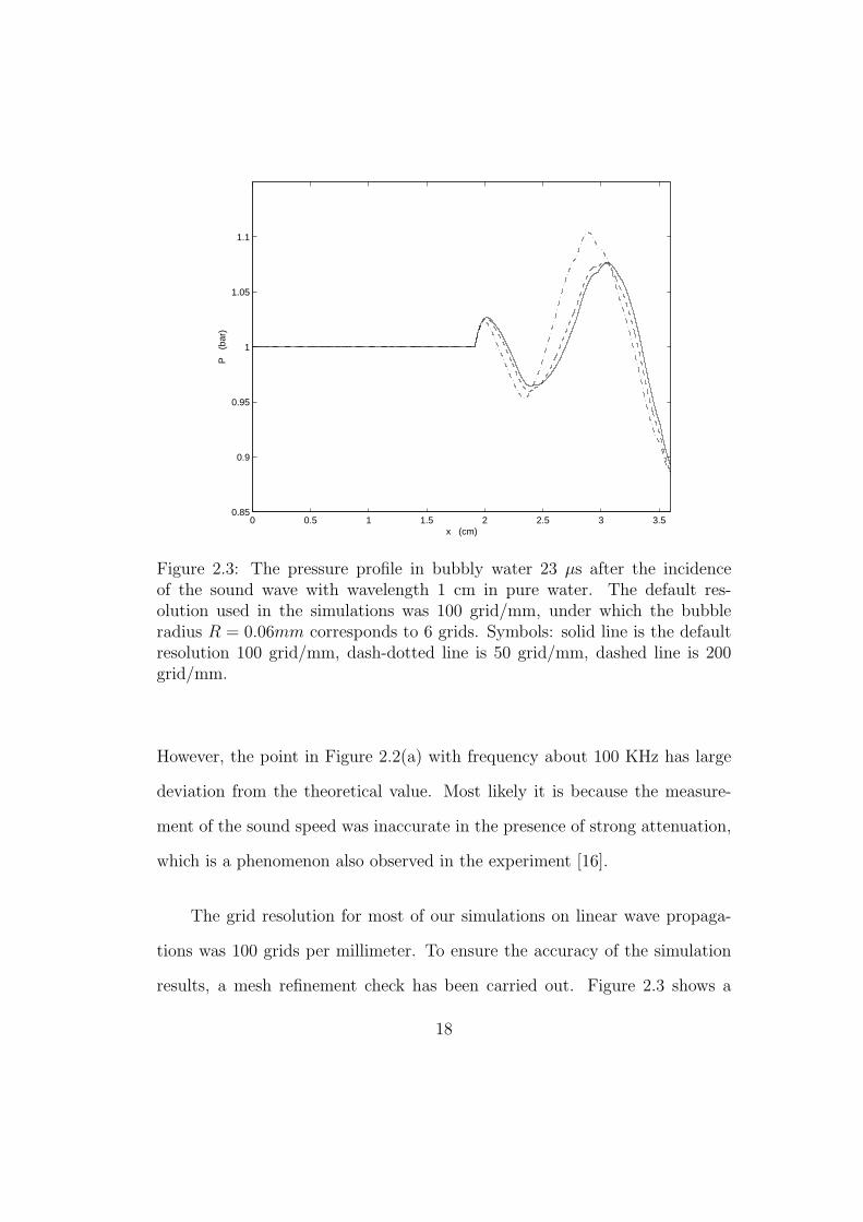
2.3 The pressure profile in bubbly water 23 µs after the incidence of
the sound wave with wavelength 1 cm in pure water. The default
resolution used in the simulations was 100 grid/mm, under which
the bubble radius R = 0.06mm corresponds to 6 grids. Symbols:
solid line is the default resolution 100 grid/mm, dash-dotted line
is 50 grid/mm, dashed line is 200 grid/mm. . . . . . . . . . . . . 18
x
2.4 The shock profiles in bubbly glycerol. The parameters in the
simulations were from the experiments [4]. pa = 1.11 bar, ρf =
1.22 g/cm3, Ra = 1.15mm. Left figures are from the simulations,
right ones are from the experiments. (a) He(γ = 1.67), β =
0.27%, Pb = 1.9bar. (b) N2(γ = 1.4), β = 0.25%, Pb = 1.7bar.
(c) SF6(γ = 1.09), β = 0.25%, Pb = 1.9bar. The curves in the
experimental figures are the author’s original fitting with artificial
turbulent viscosity. . . . . . . . . . . . . . . . . . . . . . . . . . 22
3.1 The pressure distribution right after a pulse of proton beams in
the mercury target of the Spallation Neutron Source. Courtesy
of SNS experimental facilities, Oak Ridge National Lab. . . . . . 25
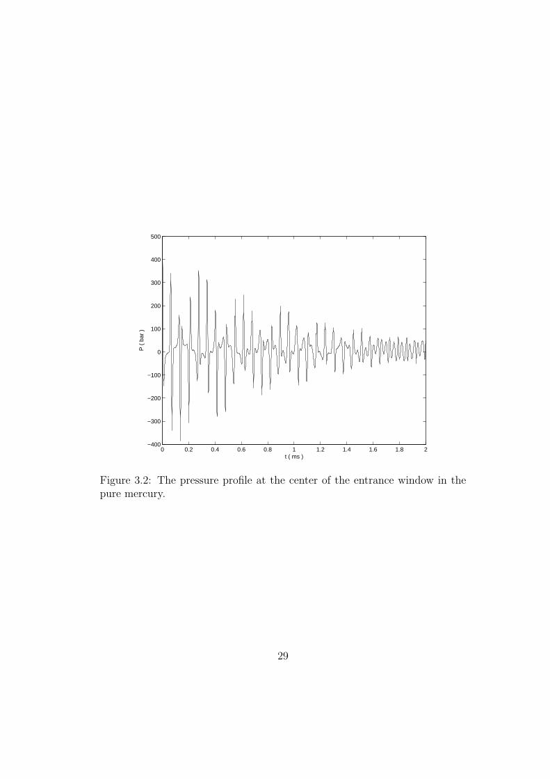
3.2 The pressure profile at the center of the entrance window in the
pure mercury. . . . . . . . . . . . . . . . . . . . . . . . . . . . . 29
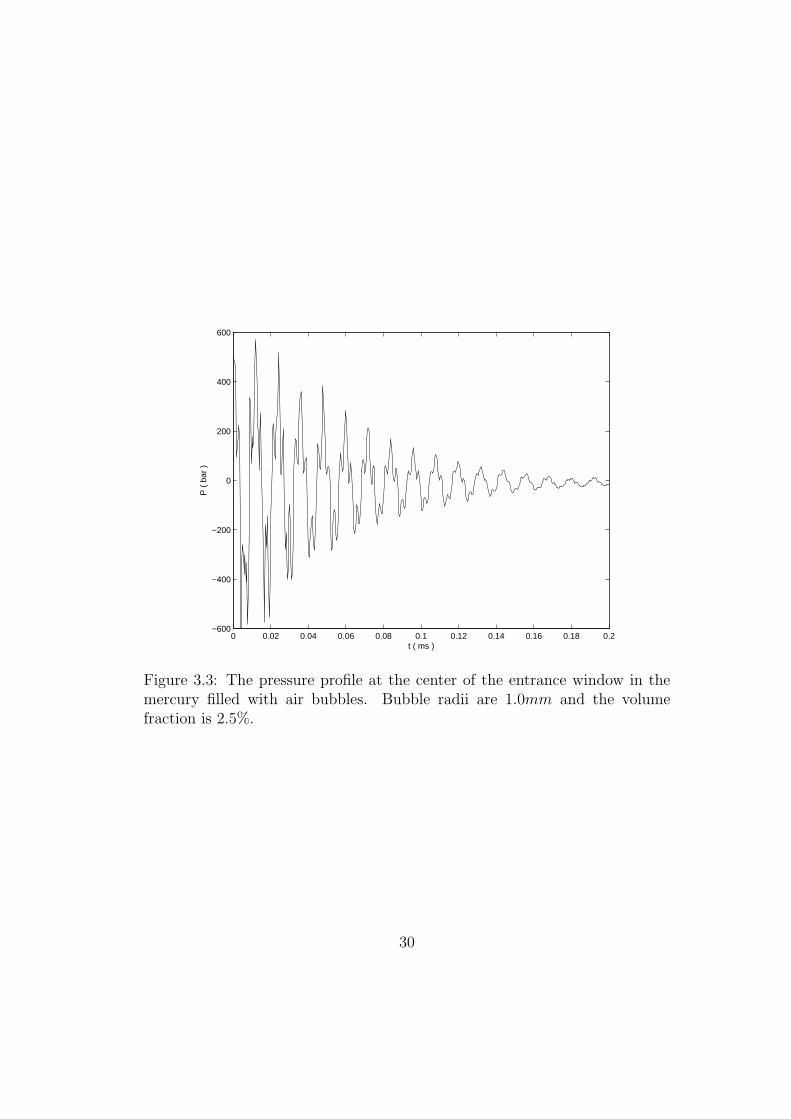
3.3 The pressure profile at the center of the entrance window in the
mercury filled with air bubbles. Bubble radii are 1.0mm and the
volume fraction is 2.5%. . . . . . . . . . . . . . . . . . . . . . . 30
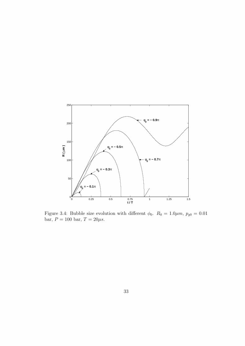
3.4 Bubble size evolution with different φ0. R0 = 1.0µm, pg0 = 0.01
bar, P = 100 bar, T = 20µs. . . . . . . . . . . . . . . . . . . . . 33
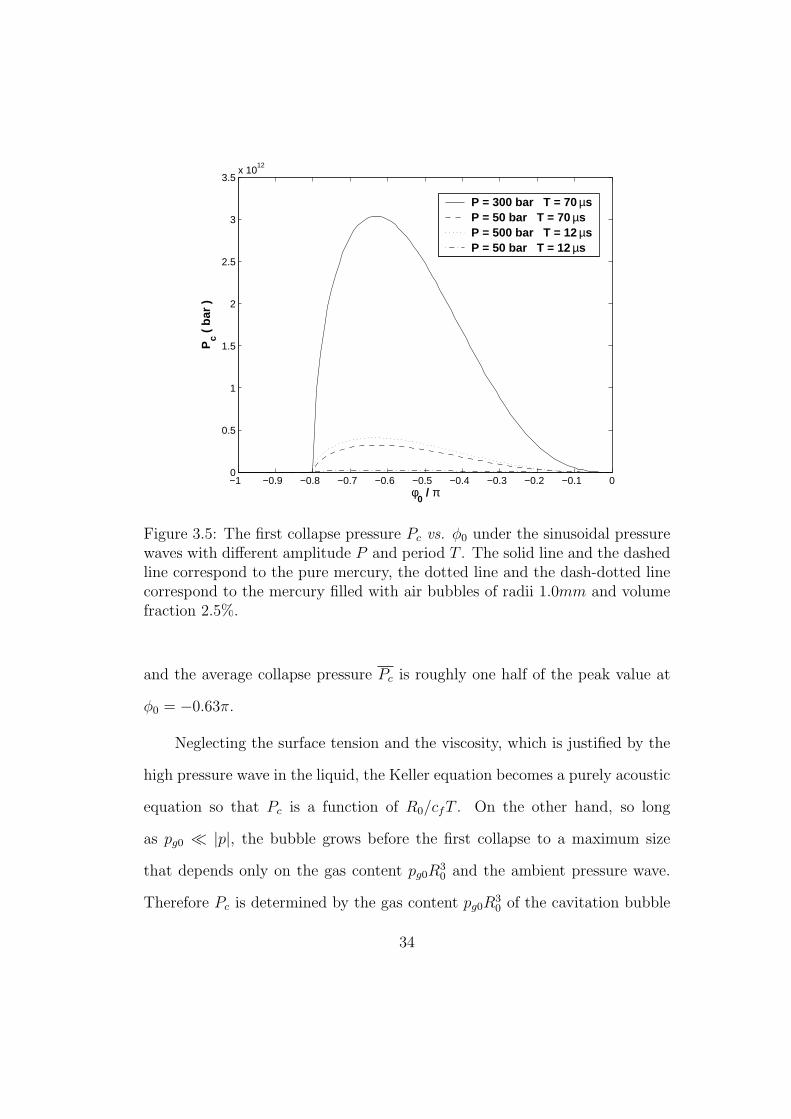
3.5 The first collapse pressure Pc vs. φ0 under the sinusoidal pressure
waves with different amplitude P and period T . The solid line
and the dashed line correspond to the pure mercury, the dotted
line and the dash-dotted line correspond to the mercury filled
with air bubbles of radii 1.0mm and volume fraction 2.5%. . . . 34
xi
4.1 The characteristics of the linearized equations for two-phase flows. 54
4.2 Pressure and velocity fields with initial conditions and parameters
given in Eqs. (4.31) and (4.32). (a) is p(x), (b) is u(x). In both
figures, dotted line is for t = 0+, dashed line is for t = 0.1, solid
line is for t = 1. . . . . . . . . . . . . . . . . . . . . . . . . . . . 58
4.3 Pressure and velocity fields with various thermal conductivity.
(pl0, ul0, Tl0) = (0, 0, 1), (pr0, ur0, Tr0) = (0, 0, 0). (Γ, ρcp, c, m)l =
(1, 1, 1, 1), (Γ, ρcp, c, m)r = (0.5, 0.5, 0.5, 1). (a) is p(x) at t = 1,
(b) is u(x) at t = 1. In both figures, dotted line is for κl = 1 and
κr = 0.5, dashed line is for κl = 0.1 and κr = 0.05, solid line is
for κl = 0.01 and κr = 0.005. . . . . . . . . . . . . . . . . . . . . 60
4.4 Schematic of the eight lemmas. Each line corresponds to a lemma.
The number on each line is the normalized integral of Txx along
the characteristic, or equivalently, the normalized ∆Th of the Rie-
mann invariants. . . . . . . . . . . . . . . . . . . . . . . . . . . 73
4.5 Pressure and velocity fields as t → 0. Initial conditions and pa-
rameters except κl and κr are given in Eqs. (4.31) and (4.32).
(a) is p(x), (b) is u(x). In both figures, dotted line is at t = 1
for κl = 1 and κr = 0.5, dashed line is at t = 0.2 for κl = 5 and
κr = 2.5, solid line is at t = 0.01 for κl = 100 and κr = 50. . . . 80
4.6 Analytical solution with initial condition and parameters given in
Eq. (4.36). (a) is T (t, x), (b) is p(t, x), and (c) is u(t, x). . . . . 85
xii
4.7 Hyperbolic and parabolic fields with various thermal conductivity.
(pl0, ul0, Tl0) = (0, 0, 1),(pr0, ur0, Tr0) = (1, 0, 0). (βT, ρcp, c, m)l =
(1, 1, 1, 1), (βT, ρcp, c,m)r = (1, 0.5, 0.5, 1). (a) is p(x) and u(x)
at t = 1, independent of κ’s. Solid line is p, dashes line is u. (b)
is T (x) at t = 1. Dotted line is for κl = 1 and κr = 2, dashed line
is for for κl = 0.01 and κr = 0.02, solid line is for for κl = 0.0001
and κr = 0.0002. . . . . . . . . . . . . . . . . . . . . . . . . . . 90
4.8 Temperature field as t → 0. Parameters and initial conditions are
the same as in Figure 4.7. Dotted line is at t = 2 for κl = 0.5 and
κr = 1, dashed line is at t = 0.5 for κl = 2 and κr = 4, solid line
is at t = 0.1 for κl = 10 and κr = 20. . . . . . . . . . . . . . . . 94
4.9 Construction of the mid state and the wave structure for the
isothermal Riemann problem. The curves passing point L is the
left shock curve (upper part) and rarefaction (lower part). The
curves passing point R is the right shock curve (upper part) and
rarefaction (lower part). The intersection is the instantaneous
mid state for contact with thermal conduction. . . . . . . . . . . 103
4.10 Schematic of interface states for travelling wave solutions of the
Euler equations with phase transitions. The states stay on the
line connecting the liquid and vapor states at the interface. . . . 109
4.11 Schematic of the travelling wave solution to the Euler equations
with heat conduction for the left shock wave. . . . . . . . . . . . 112
xiii
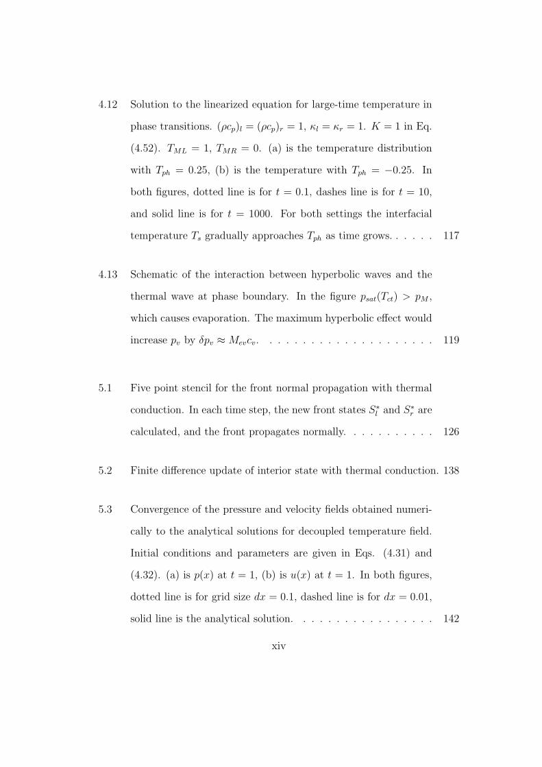
4.12 Solution to the linearized equation for large-time temperature in
phase transitions. (ρcp)l = (ρcp)r = 1, κl = κr = 1. K = 1 in Eq.
(4.52). TML = 1, TMR = 0. (a) is the temperature distribution
with Tph = 0.25, (b) is the temperature with Tph = −0.25. In
both figures, dotted line is for t = 0.1, dashes line is for t = 10,
and solid line is for t = 1000. For both settings the interfacial
temperature Ts gradually approaches Tph as time grows. . . . . . 117
4.13 Schematic of the interaction between hyperbolic waves and the
thermal wave at phase boundary. In the figure psat(Tct) > pM ,
which causes evaporation. The maximum hyperbolic effect would
increase pv by δpv ≈ Mevcv. . . . . . . . . . . . . . . . . . . . . 119
5.1 Five point stencil for the front normal propagation with thermal
conduction. In each time step, the new front states S∗l and S∗r are
calculated, and the front propagates normally. . . . . . . . . . . 126
5.2 Finite difference update of interior state with thermal conduction. 138
5.3 Convergence of the pressure and velocity fields obtained numeri-
cally to the analytical solutions for decoupled temperature field.
Initial conditions and parameters are given in Eqs. (4.31) and
(4.32). (a) is p(x) at t = 1, (b) is u(x) at t = 1. In both figures,
dotted line is for grid size dx = 0.1, dashed line is for dx = 0.01,
solid line is the analytical solution. . . . . . . . . . . . . . . . . 142
xiv
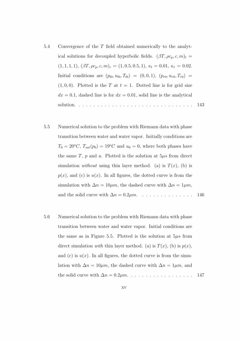
5.4 Convergence of the T field obtained numerically to the analyt-
ical solutions for decoupled hyperbolic fields. (βT, ρcp, c, m)l =
(1, 1, 1, 1), (βT, ρcp, c, m)r = (1, 0.5, 0.5, 1), κl = 0.01, κr = 0.02.
Initial conditions are (pl0, ul0, Tl0) = (0, 0, 1), (pr0, ur0, Tr0) =
(1, 0, 0). Plotted is the T at t = 1. Dotted line is for grid size
dx = 0.1, dashed line is for dx = 0.01, solid line is the analytical
solution. . . . . . . . . . . . . . . . . . . . . . . . . . . . . . . . 143
5.5 Numerical solution to the problem with Riemann data with phase
transition between water and water vapor. Initially conditions are
T0 = 20oC, Tsat(p0) = 19oC and u0 = 0, where both phases have
the same T , p and u. Plotted is the solution at 5µs from direct
simulation without using thin layer method. (a) is T (x), (b) is
p(x), and (c) is u(x). In all figures, the dotted curve is from the
simulation with ∆n = 10µm, the dashed curve with ∆n = 1µm,
and the solid curve with ∆n = 0.2µm. . . . . . . . . . . . . . . 146
5.6 Numerical solution to the problem with Riemann data with phase
transition between water and water vapor. Initial conditions are
the same as in Figure 5.5. Plotted is the solution at 5µs from
direct simulation with thin layer method. (a) is T (x), (b) is p(x),
and (c) is u(x). In all figures, the dotted curve is from the simu-
lation with ∆n = 10µm, the dashed curve with ∆n = 1µm, and
the solid curve with ∆n = 0.2µm. . . . . . . . . . . . . . . . . . 147
xv
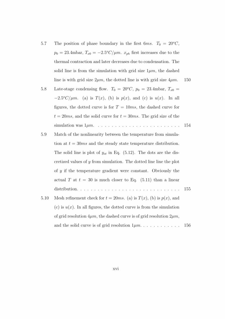
5.7 The position of phase boundary in the first 6ms. T0 = 20oC,
p0 = 23.4mbar, Tx0 = −2.5oC/µm. xph first increases due to the
thermal contraction and later decreases due to condensation. The
solid line is from the simulation with grid size 1µm, the dashed
line is with grid size 2µm, the dotted line is with grid size 4µm. 150
5.8 Late-stage condensing flow. T0 = 20oC, p0 = 23.4mbar, Tx0 =
−2.5oC/µm. (a) is T (x), (b) is p(x), and (c) is u(x). In all
figures, the dotted curve is for T = 10ms, the dashed curve for
t = 20ms, and the solid curve for t = 30ms. The grid size of the
simulation was 1µm. . . . . . . . . . . . . . . . . . . . . . . . . 154
5.9 Match of the nonlinearity between the temperature from simula-
tion at t = 30ms and the steady state temperature distribution.
The solid line is plot of yst in Eq. (5.12). The dots are the dis-
cretized values of y from simulation. The dotted line line the plot
of y if the temperature gradient were constant. Obviously the
actual T at t = 30 is much closer to Eq. (5.11) than a linear
distribution. . . . . . . . . . . . . . . . . . . . . . . . . . . . . . 155
5.10 Mesh refinement check for t = 20ms. (a) is T (x), (b) is p(x), and
(c) is u(x). In all figures, the dotted curve is from the simulation
of grid resolution 4µm, the dashed curve is of grid resolution 2µm,
and the solid curve is of grid resolution 1µm. . . . . . . . . . . . 156
xvi
List of Tables
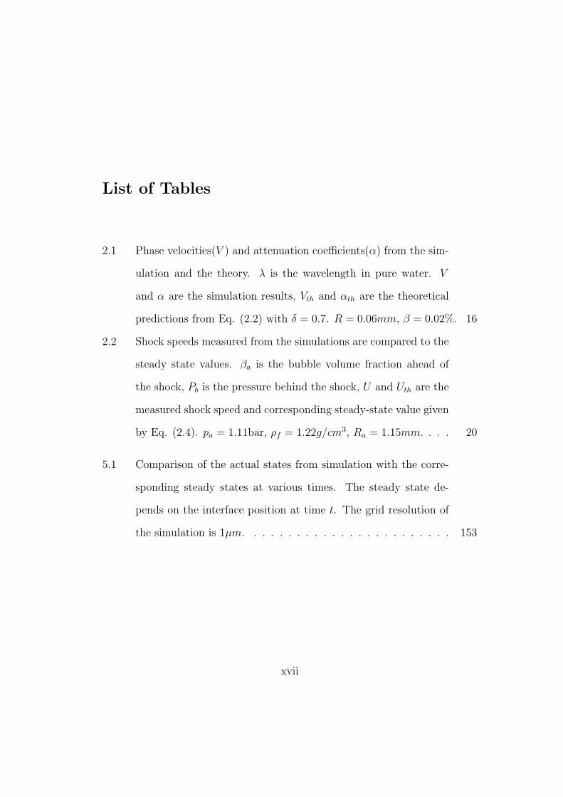
2.1 Phase velocities(V ) and attenuation coefficients(α) from the sim-
ulation and the theory. λ is the wavelength in pure water. V
and α are the simulation results, Vth and αth are the theoretical
predictions from Eq. (2.2) with δ = 0.7. R = 0.06mm, β = 0.02%. 16
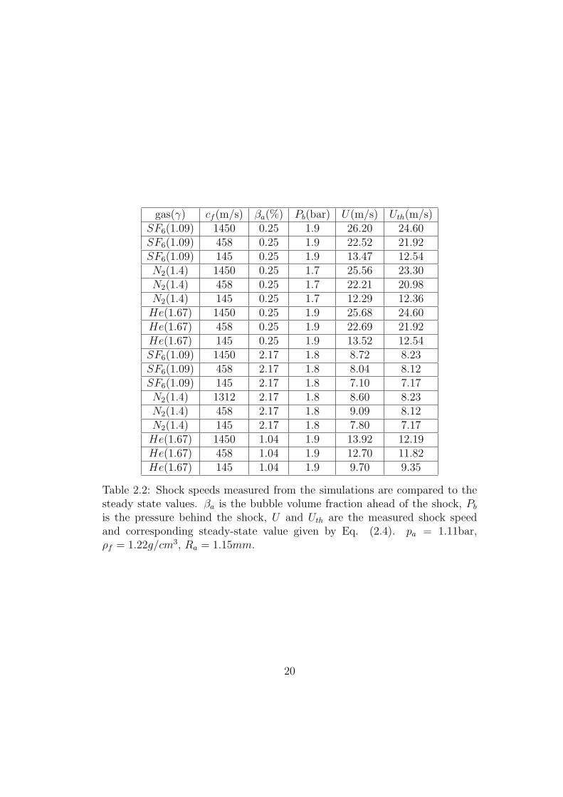
2.2 Shock speeds measured from the simulations are compared to the
steady state values. βa is the bubble volume fraction ahead of
the shock, Pb is the pressure behind the shock, U and Uth are the
measured shock speed and corresponding steady-state value given
by Eq. (2.4). pa = 1.11bar, ρf = 1.22g/cm3, Ra = 1.15mm. . . . 20
5.1 Comparison of the actual states from simulation with the corre-
sponding steady states at various times. The steady state de-
pends on the interface position at time t. The grid resolution of
the simulation is 1µm. . . . . . . . . . . . . . . . . . . . . . . . 153
xvii
Acknowledgements
I would like to express my profound gratitude to my advisor, Doctor
James Glimm, for his advice, support and guidance toward my Ph. D. degree.
He taught me not only the way to do scientific research, but also the way to
become a professional scientist. He is my advisor and a lifetime role model for
me.
I am also deeply indebted to the support of Doctor Roman Samulyak,
especially for suggesting this important and exciting thesis topic. His scientific
vigor and dedication makes him a great mentor and a good friend.
I would like to thank Drs. Xiaolin Li, Zhiliang Xu and Yongming Zhang,
from whom I have learned many important scientific and mathematical skills.
Work has been more productive and life a little easier thanks to them.
I would also like to thank all my friends for their friendship and encour-
agement during my four year study as a graduate student at Stony Brook. It
has been great to have so many friends who can share my problem and hap-
piness, only a few yards away. In particular, I would like to mention Xinfeng
Liu and Jinjie Liu. They have shared with me many interesting and inspiring
ideas.
Throughout my academic career, the constant support of my parents and

my wife has always motivated me to strive forward. The unconditional love
of my parents has never been affected by the physical distance between us.
Without my wife, dear Xiyue, I could never have been able to accomplish the
work as torturing as writing a thesis. Last but not least, I want to thank my
one-year-old daughter Vivian for cheering me up from the exhaustion after
weeks of continuous work by calling me daddy. My dissertation is dedicated
to them.
During my years here at Stony Brook I have grown and matured both
personally and professionally. I am grateful to have gone through it all, and
I look forward to what comes next. I thank all who have helped me through
this leg of journey.
Chapter 1
Introduction
1.1 Direct Numerical Simulation of Bubbly Flows
Wave propagation in bubbly fluids has attracted investigators for many
decades because of its special properties. Bubbly fluids have the unique fea-
ture that even a minute bubble concentration (volume fraction less than one
percent) increases the compressibility of the system drastically. The system
transports energy at a speed considerably lower than the sound speeds in both
phases as a result of the energy exchange between the liquid and the bubbles.
When additional effects such as vaporization and condensation play a role,
e.g. in cavitating flows, further phenomena, still little understood, are super-
imposed upon the basic behavior of bubbly flows. The rich internal structure
of bubbly flows endows the medium strikingly complex behavior.
One of the reasons for the study of bubbly flows is their wide applications
ranging from hydraulic engineering to high energy physics experiments. In
particular, we are interested in a recent application of bubbly fluids in the
mitigation of cavitation damages in the Spallation Neutron Source (SNS)[1],
1
which will be discussed in details in Chapter 3. Another important moti-
vation is to connect the microscopic behavior of individual bubbles to the
macroscopic behavior of the mixed medium that one directly observes. Since
the microstructure in this case is made up of a complex substructure, the task
is much more complicated than that of classical kinetic theory.
The wave propagation in bubbly fluids has been studied using a variety
of methods. Extensive investigation has been done on the subject based on
various mathematical models. Significant progress has been achieved on the
study of systems consisting of non-condensable gas bubbles (see for example
[46, 6, 4, 44]) and of vapor bubbles (see for example [15, 24]). The treatment
of the kinetic and thermal properties of the medium, e.g. the compressibility
of the liquid and the thermal conduction, by different authors varies. But they
shared a common feature that the two phases were not separated explicitly,
i.e. the bubble radius and concentration were considered as functions of time
and space. The Rayleigh-Plesset equation or the Keller equation governing
the evolution of spherical bubbles has been used as the kinetic connection be-
tween the bubbles and fluid. These models include many important physical
effects in bubbly systems such as the viscosity, the surface tension and thermal
conduction. Numerical simulations of such systems requires relatively sim-
ple algorithms and are computational inexpensive. Nevertheless, such models
treat the system as a pseudo-fluid and cannot capture all features of the rich
internal structure of the bubbles. They exhibit sometimes large discrepancies
with experiments [44] even for systems of non-condensable gas bubbles. These
models are also not suitable if the bubbles are distorted severely by the flow or
2
even fission into smaller bubbles, as it may happen in cavitating and boiling
flows [7, 13].
A powerful method for the multiphase problem, direct numerical simula-
tion (DNS), is based on techniques developed for free surface flows. Welch [45]
investigated numerically the evolution of a single vapor bubble using interface
tracking method. Juric and Tryggvason [29] simulated the boiling flows using
the incompressible flow approximation for both liquid and vapor and a sim-
plified version of interface tracking. In the thesis, we describe a DNS method
for the simulation of bubbly fluid using front tracking. Our FronTier code is
capable of tracking and resolving topological changes of a large number of in-
terfaces in two- and three-dimensional spaces. Both the bubbles and the fluid
are compressible in the simulation because we are interested in the speed of
wave propagations. We simulated the propagation of acoustic and shock waves
in bubbly fluids and compared them with the theory and the experiments in
Chapter 2.
After the validation of the FronTier code on the bubbly flows, it was
applied to the engineering problem of cavitation mitigation in the Spallation
Neutron Source. In Chapter 3, after the description of SNS and the related
bubble injection technique for the mitigation of the cavitation, the problem was
tackled in two steps. First, the pressure wave propagation in the container of
the mercury target for the SNS was simulated using the front tracking method.
Then the collapse pressure of cavitation bubbles was calculated by solving
the Keller equation under the ambient pressure whose profile was obtained
in the first step. Finally the efficiency of the cavitation damage mitigation
3
was estimated by comparing the average collapse pressure with and without
injected bubbles.
1.2 Interfacial Dynamics of Phase Transitions
The dynamics of gas bubbles and the wave propagation in fluid filled with
non-condensable bubbles have been investigated theoretically and experimen-
tally for many decades, but the research on the corresponding problem for
vapor bubbles is relatively new and the understanding is less developed. The
interest on the dynamics of vapor bubbles is twofold.
Due to the large amount of energy absorbed or liberated in the form of
latent during phase transitions, boiling and condensation are key processes
in the extraction of energy from fuels for daily life. Heat exchanger equip-
ment and piping in power plants and oil refineries are examples of traditional
applications. A more recent issue coming from the space shuttles is the en-
hancement of heat transfer during boiling in microgravity. Another area that
phase transitions play an important role is the cavitating flows, e.g. in the jet
simulation in a diesel engine [22]. All these applications require detailed under-
standing of the phase transition process. Despite its importance and the vast
body of research on boiling, the fundamental physical mechanisms involved are
far from being understood, as pointed out by Juric et. al. [29] and Welch[45].
Not much experimental measurement on the dynamics of phase transitions is
available because of the small time and spatial scale of the process.
The dynamics of phase transitions is of great scientific interest too. An-
alytical and numerical efforts to understand the boiling have been focused
4
mainly on simple models of vapor bubble dynamics until recently. Rayleigh
[41] formulated a simplified equation of motion for inertia controlled growth
of a spherical vapor bubble. Plesset and Zwick [37] and later Prosperetti and
Plesset [40], among others, extended Rayleigh’s analysis. Most models have
been based on the Rayleigh-Plesset equation for incompressible liquid or the
Keller equation of first order in c−1l for weakly compressible liquid. Phase tran-
sitions with full compressibility of both phases have been discussed by Menikoff
and Plohr [36] with the transition zone treated as the macroscopic mixture of
the two phases at equilibrium. More recently, Welch [45] studied the two-phase
flows including interface tracking with mass transfer while the phase interface
was assumed to exist in thermal and chemical (Gibbs potential) equilibrium.
Juric and Tryggvason [29] simulated the boiling flows in incompressible fluids
using the non-equilibrium phase transition model with a parameter called ki-
netic mobility whose value was measured experimentally. Hao and Prosperetti
[24] investigated the dynamics of bubbles in acoustic pressure fields assuming
the vapor was saturated. Matsumoto and Takemura [35] studied numerically
the influence of internal phenomena on gas bubble motion with complete mass,
momentum and energy conservation laws for compressible fluids and the in-
terfacial dynamics of phase transitions, in which they referred to the value
0.4 for the evaporation coefficient measured by Hatamiya and Tanaka [25].
Later Preston, Colonius and Brennen [2], in the development of simpler and
more efficient bubble dynamic models that capture the important aspects of
the diffusion precesses, computed the growth and collapse of a vapor bubble
under pressure waves in incompressible liquid with the interfacial dynamics of
5
phase transitions using a Chebychev spectral method to solve the temperature
equation for the bubble.
The equations of the conservation laws and the interfacial dynamics of
phase transitions have been studied numerically by the authors listed above.
Hao and Prosperetti also investigated the linear theory of bubble oscillation
in acoustic waves. However, the system of non-equilibrium phase transitions,
as far as we know, has not been studied as a problem with Riemann data.
As a contrast, the Riemann problem for reacting gas has been studied exten-
sively [43]. For combustion flows, the energy difference between the phases
(burnt and unburnt) is a fixed constant, namely, the heat released or absorbed
in the chemical reaction, so the Riemann problem has not been changed by
much. While for phase transitions, there is complicated interfacial dynamics
involving the latent heat and Clausius-Clapeyron equation. Furthermore, the
heat conduction makes the conservational laws no longer purely hyperbolic,
thus the solution to the problem with Riemann data does not have the self
similarity in the classical Riemann solution. In the adiabatic limit (thermal
conductivity goes to zero), according to the theory of viscous profile, the so-
lution should approach the Riemann solution, which we will show is correct
for nonlinear equations but not for linearized equations. The theory of viscous
profile usually deals with a hyperbolic field coupled to its own parabolic equa-
tion, while for Euler equations with thermal conduction the hyperbolic fields
(pressure and velocity) are coupled to a different parabolic field (temperature),
which complicates the problem by allowing jump discontinuity in certain fields
while disallowing in others. The qualitative and quantitative properties of the
6
solution to the phase transition problem with Riemann data are our main sub-
jects. The simpler case of two immiscible thermal conductive fluids was also
investigated, in which the interface between the two fluids was a contact with
thermal flux, or the so called thermal contact.
In Chapter 4 we analyzed the interfacial dynamics of phase transitions
and the wave equations for immiscible fluids. The phase transition rate is
associated by the kinetic theory with the deviation of the vapor pressure from
the saturated pressure. Analytical solutions to the linearized equations have
been explored. The adiabatic and the isothermal limits have been investigated
for both the linearized and the nonlinear equations, for latter the method of
travelling wave solutions has been used. The wave structure of the solution to
the problem with Riemann data has been discussed.
In Chapter 5 we implemented a numerical scheme for solving the Euler
equations with thermal conduction and phase transitions in the frame of front
tracking. Heat conduction has been added to the interior state update with
second order accuracy. Phase boundary propagation has been handled accord-
ing to the interfacial dynamics. A numerical technique has been introduced
to account for the thermal layer thinner than a grid cell. The algorithm has
been validated and applied to sample physical problems.
7
Chapter 2
Direct Numerical Simulation of Bubbly Flows
In Section 2.1, we give a brief review of the theory and the experiments on
bubbly flows. Section 2.2 is the description of the numerical method. Section
2.3 lists the results of the direct numerical simulations on linear and shock
wave propagations in bubbly fluids along with the comparison to the theory
and the experiments.
2.1 Theory and Experiments on Bubbly Flows
2.1.1 Wave Equations
The theory on bubbly flows is based on the homogenized model, in which
the fluid and the bubbles are treated a single mixed phase, as opposed to
the two separated phases in the direct numerical simulations. In compressible
fluids with gas bubbles, the conservation of mass and momentum in one spatial
8
dimension give
1
ρfc2f
∂p
∂t+
∂u
∂x=
∂β
∂t,
∂(ρu)
∂t+
∂(ρu2 + p)
∂x= 0,
where β is the bubble volume fraction, and ρ is the averaged density of the
mixed phase that equals ρf (1 − β) + ρgβ. The bubble oscillation in weakly
compressible fluids is governed by the Keller equation [31, 32, 39],
(1− 1
cf
dR
dt)R
d2R
dt2+
3
2(1− 1
3cf
dR
dt)(
dR
dt)2 =
1
ρf
(1+1
cf
dR
dt+
R
cf
d
dt)(pB−p). (2.1)
The bubble pressure pg is approximately uniform except for sound waves of
frequency far above the resonance. For bubbles of diameter 0.1mm and above,
the thermal diffusivity ν << ωR2 except for sound waves of frequency far
below resonance. Therefore the bubbles are almost adiabatic for near-resonant
sound waves. For bubbles consisting of γ-law gases,
pgR3γ = constant.
Neglecting the viscosity, the difference between pg and pB, the liquid pressure
at the bubble surface, is from the surface tension,
pg = pB +2σ
R.
9
2.1.2 Linear Waves
The following dispersion relation for linear sound waves in bubbly fluids
was derived from the wave equations [46].
k2
ω2=
1
c2f
+1
c2
1
1− iδ ωωB− ω2
ω2B
, (2.2)
where ωB is the resonant frequency of single bubble oscillation, δ is the damp-
ing coefficient accounting for the various dissipation mechanisms. cf is the
sound speed in bubble free fluid and c is the sound speed in the low-frequency
limit, which is given by
1
c2= (βρg + (1− β)ρf )(
β
ρgc2g
+1− β
ρgc2f
),
where ρg and ρf are the densities of the gas and the fluid, cg and cf are the
sound speeds of the two phases. For adiabatic bubbles,
c =
√γp
βρf
,
ωB =1
R
√3γp
ρf
. (2.3)
Chapman and Plesset [8] formulated δ as the sum of the acoustic, viscous
and thermal contributions. It has been pointed out by Prosperetti et. al.
[38, 12] that δ depends on the frequency of the sound wave. Nevertheless, Eq.
(2.2) has been widely used for the dispersion relation. The dispersion relation
for near-resonant sound waves measured in different experiments [16, 34, 42]
10
agreed with the theoretical predictions.
2.1.3 Shock Waves
The shock profile in the bubbly fluid evolves into a smooth steady form in
contrast to the sharp discontinuity in the pure fluid. The steady state shock
speed was obtained from the Rankine-Hugoniot relation [44],
1
U2=
1
c2f
+ ρfβb − βa
Pa − Pb
where subscripts a and b stand for ahead and behind the shock front. The
steady state reaches thermal equilibrium, so for ideal gas bubbles with surface
tension neglected, Paβa = Pbβb. Therefore
1
U2=
1
c2f
+ ρfβa
Pb
(2.4)
The evolution into a steady wave can take very long time and distance, and
the unsteady waves move at higher velocities [44]. The shock profiles were
measured for various gas bubbles by Beylich and Gulhan [4].
2.2 Numerical Method
We have been studying bubbly fluids as a system of one-phase domains
separated by free interfaces using FronTier, a front tracking compressible hy-
drodynamics code. Front tracking is an adaptive computational method in
which a lower dimensional moving grid is fit to and follows distinguished waves
11
in a flow. The front propagates according to the dynamics around it (i.e. La-
grangian) while the regular spatial grid is fixed in time (i.e. Eulerian). The
discontinuities across the interfaces are kept sharp so as to eliminate the inter-
facial numerical diffusion which plagues traditional finite difference schemes.
In each time step, the front is first propagated then the interior states are
updated. For the front propagation, the interfaces are first propagated in the
normal direction for each point on the fronts and the states on either side evolve
according to the solution of non-local Riemann problems. The hyperbolic
solver has three steps: slope reconstruction, prediction using local Riemann
solver, and correction by nonlocal solver. Then the states on the propagated
fronts are updated in the tangential direction while the fronts are fixed. After
that the fronts are tested for intersection and then untangled or redistributed
if necessary to resolve the topological change or the clustering/sparsity of grid
points on the interfaces due to front contract/expand.
For the subsequent interior state update, FronTier uses high resolution
shock-capturing hyperbolic schemes on a spatial grid. Among the various
shock capturing methods currently implemented in FronTier, a second order
monotone upwind scheme for conservation laws (MUSCL) scheme developed
by Van Leer and adapted for FronTier by I-L. Chern was used for the sim-
ulation here. MUSCL scheme is similar to the piecewise parabolic method
described in [11], and a detailed description can be found in [10]. The two-
pass implementation currently being used in FronTier, namely, first regular
cells then irregular cells update, is well documented in [21]. Different equation
of state models are used for gas/vapor bubbles and the ambient fluid.
12
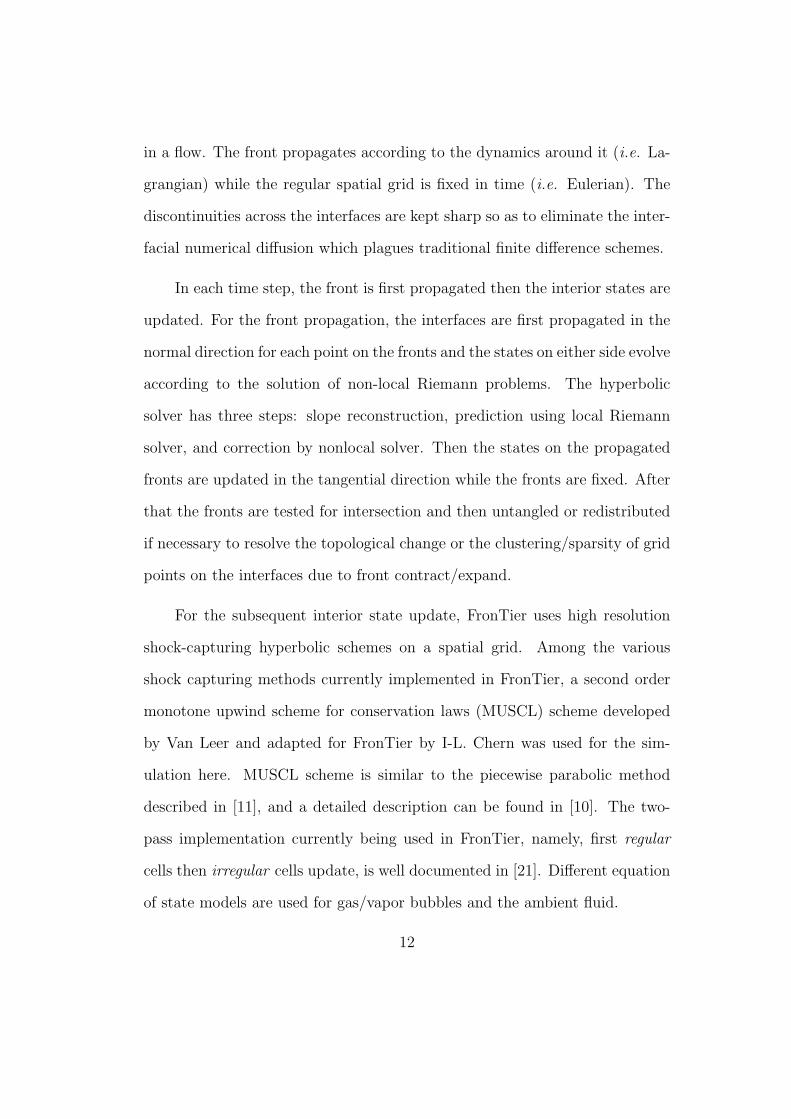
Incident acoustic or shock wave Computational domain
Tracked surface bubblesLiquid
Figure 2.1: Schematic of the numerical experiments on the propagation oflinear and shock waves in bubbly fluids.
FronTier can handle multidimensional wave interactions in both two- [20]
and three- [19] dimensional spaces. Although computationally intensive, front
tracking is potentially very accurate in treating many physical effects in bubbly
flows, such as the compressibility of the fluid, surface tension and viscosity.
Since the FronTier code is capable of tracking simultaneously a large num-
ber of interfaces and resolving their topological changes, many effects that
are difficult to handle in mathematical models for bubbly flows are now nat-
urally included in the simulations, e.g. the bubbles’ deviation from spheric-
ity, bubble-fluid relative motion, bubble merge/fissure and bubble size/spatial
distribution. This approach has numerous potential advantages for modelling
the phase transitions in boiling and cavitation flows. We have implemented
a model for the phase transitions induced mass transfer across free interfaces
[22]. FronTier is implemented for distributed memory parallel computers.
For the application of FronTier to the simulation of bubbly flows, the
13
region around a long column of bubbles (tens to hundreds) has been chosen as
the computational domain, as shown in Figure 2.1. Two approximations were
used in the simulations. The flow inside the column was assumed to be ax-
isymmetric and the influence from the neighboring bubbles was approximated
by the Neumann boundary condition on the domain wall. Thus the wave
propagation in bubbly flows was reduced to an axisymmetric two-dimensional
problem. An extensive introduction to the FronTier code for axisymmetric
flows can be found in [21].
The axisymmetric flow approximation is crude although it is exact for
the scattering of the planar wave by an isolated column of bubbles that are
initially spherical. The Neumann boundary condition between adjacent bub-
bles is also too strong because the scattered pressure wave is only partially
reflected. As a contrast, the scattering theory, on which the Keller equation is
based, completely neglects the reflection between bubbles and the secondary
scattering. Therefore the scattering theory only holds for the case of small β
such that bubble interaction is negligible. For moderate β, the secondary scat-
tering can not be neglected, and the Neumann boundary condition between
adjacent bubbles is a better approximation.
2.3 Simulation Results on Bubbly Flows
In this section, we present the results of the DNS on the linear and shock
wave propagations in bubbly fluids. The dispersion relation measured from the
simulations were compared to the theory in Section 2.3.1. The shock speeds
measured from the simulations were compared to the steady-state values, and
14
the shock profiles for various gas bubbles were compared to the experiments
[4] in Section 2.3.2.
2.3.1 Linear Waves
To compare the simulation results with the theory we measured the dis-
persion relation. Writing down the complex wave number k in Eq. (2.2) as
k = k1 + ik2, we have
ei(kx−ωt) = e−k2xei(k1x−ωt),
from which the phase velocity of the sound wave is defined as
V =ω
k1
, (2.5)
and the attenuation coefficient α in dB per unit length defined as
α = 20 log10 e · k2. (2.6)
The bubble radius in the simulation was R = 0.06mm. From Eq. (2.3), we
have
fB =ωB
2π=
1
2πR
√3γp
ρf
= 54.4 KHz.
We simulated the sound waves of frequencies ranging from 30 to 300 KHz.
The volume fraction β = 0.02%. The amplitude of the pressure wave was
chosen to be 0.1 bar, one tenth of the ambient pressure. The linearity was
ensured by comparison with sound waves of half amplitude, from which the
dispersion relation measured was virtually the same. For each frequency, the
15
λ(cm) f(KHz) V (cm/ms) Vth(cm/ms) α(dB/cm) αth(dB/cm)0.5 290 155 153 2.2 0.91.0 145 183 194 5.7 5.01.5 96.7 220 274 18.4 20.72.0 72.5 160 173 28.5 30.92.5 58.0 100 100 21.8 29.42.75 52.7 75 84 18.9 25.23.0 48.3 68 75 17.8 20.44.0 36.3 62 68 10.7 8.55.0 29.0 66 69 3.9 4.4
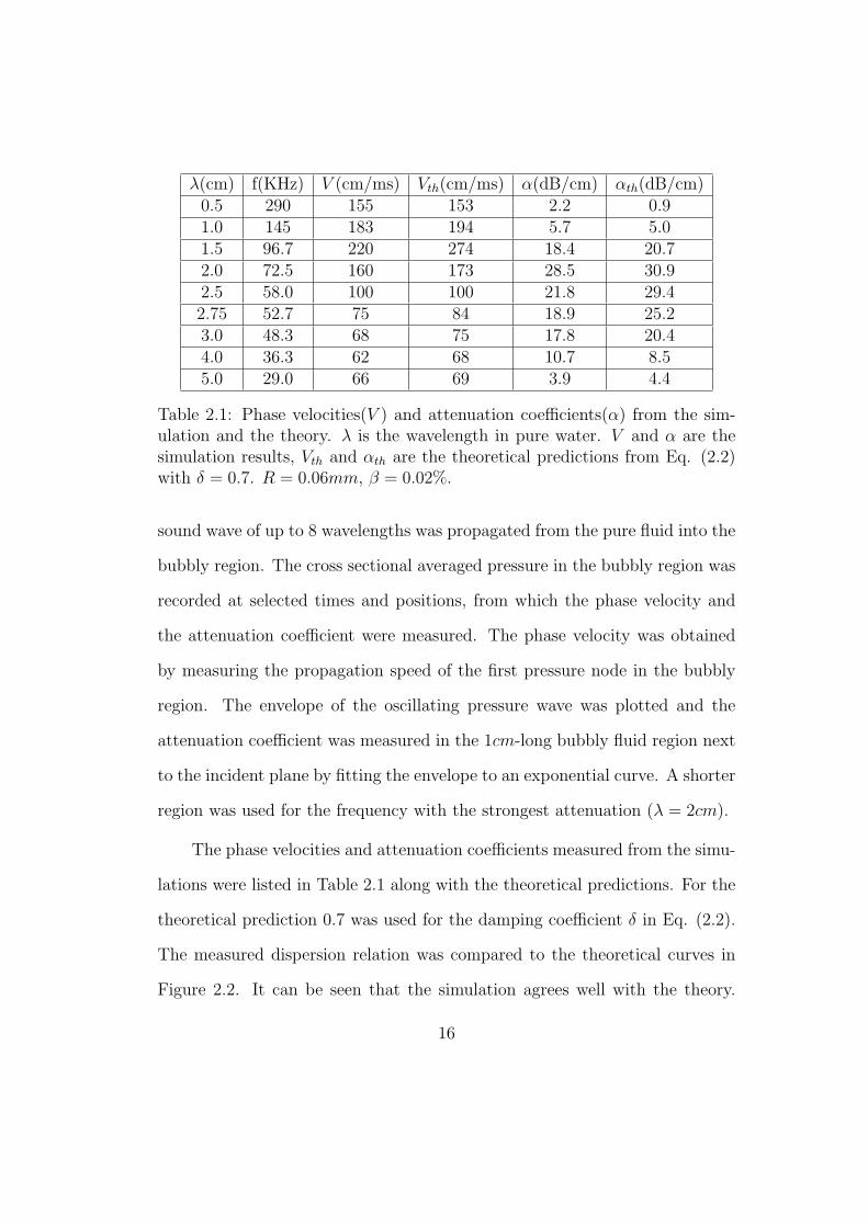
Table 2.1: Phase velocities(V ) and attenuation coefficients(α) from the sim-ulation and the theory. λ is the wavelength in pure water. V and α are thesimulation results, Vth and αth are the theoretical predictions from Eq. (2.2)with δ = 0.7. R = 0.06mm, β = 0.02%.
sound wave of up to 8 wavelengths was propagated from the pure fluid into the
bubbly region. The cross sectional averaged pressure in the bubbly region was
recorded at selected times and positions, from which the phase velocity and
the attenuation coefficient were measured. The phase velocity was obtained
by measuring the propagation speed of the first pressure node in the bubbly
region. The envelope of the oscillating pressure wave was plotted and the
attenuation coefficient was measured in the 1cm-long bubbly fluid region next
to the incident plane by fitting the envelope to an exponential curve. A shorter
region was used for the frequency with the strongest attenuation (λ = 2cm).
The phase velocities and attenuation coefficients measured from the simu-
lations were listed in Table 2.1 along with the theoretical predictions. For the
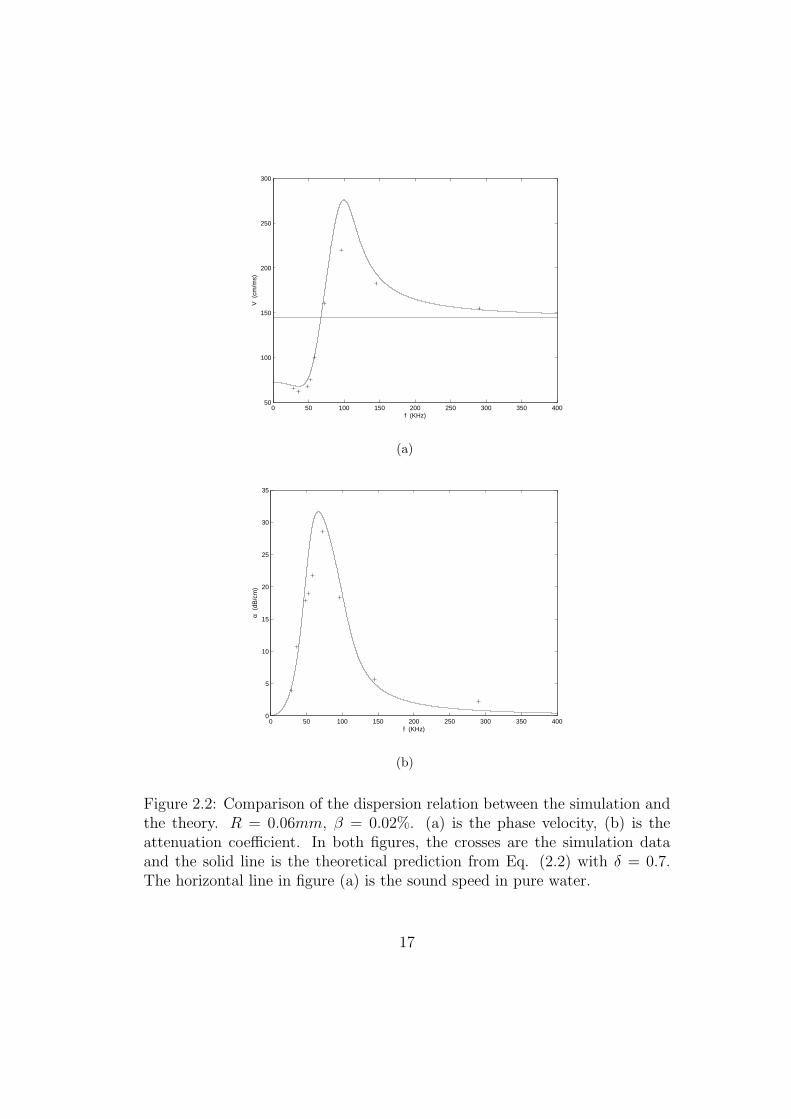
theoretical prediction 0.7 was used for the damping coefficient δ in Eq. (2.2).
The measured dispersion relation was compared to the theoretical curves in
Figure 2.2. It can be seen that the simulation agrees well with the theory.
16
0 50 100 150 200 250 300 350 40050
100
150
200
250
300
f (KHz)
V (
cm/m
s)
(a)
0 50 100 150 200 250 300 350 4000
5
10
15
20
25
30
35
f (KHz)
α (
dB/c
m)
(b)
Figure 2.2: Comparison of the dispersion relation between the simulation andthe theory. R = 0.06mm, β = 0.02%. (a) is the phase velocity, (b) is theattenuation coefficient. In both figures, the crosses are the simulation dataand the solid line is the theoretical prediction from Eq. (2.2) with δ = 0.7.The horizontal line in figure (a) is the sound speed in pure water.
17
0 0.5 1 1.5 2 2.5 3 3.50.85
0.9
0.95
1
1.05
1.1
x (cm)
P
(bar
)
Figure 2.3: The pressure profile in bubbly water 23 µs after the incidenceof the sound wave with wavelength 1 cm in pure water. The default res-olution used in the simulations was 100 grid/mm, under which the bubbleradius R = 0.06mm corresponds to 6 grids. Symbols: solid line is the defaultresolution 100 grid/mm, dash-dotted line is 50 grid/mm, dashed line is 200grid/mm.
However, the point in Figure 2.2(a) with frequency about 100 KHz has large
deviation from the theoretical value. Most likely it is because the measure-
ment of the sound speed was inaccurate in the presence of strong attenuation,
which is a phenomenon also observed in the experiment [16].
The grid resolution for most of our simulations on linear wave propaga-
tions was 100 grids per millimeter. To ensure the accuracy of the simulation
results, a mesh refinement check has been carried out. Figure 2.3 shows a
18
typical result. It can be seen that the results were reasonably accurate at the
default grid resolution (100 grid/mm). It has also been noticed that near the
resonant frequency fB the resolution requirement is higher. More specifically,
higher resolution would give larger attenuation coefficients, which explains in
part why the points in the Figure 2.2(b) are all below the theoretical curve
near the peak. Another important reason for the deviation is, as pointed out
by Prosperetti et. al. [38, 12], the dependence of δ on the frequency. The sim-
plification used in the simulation, such as axisymmetric approximation and
Neumann boundary condition, also contributed to the error.
2.3.2 Shock Waves
Beylich and Gulhan [4] studied the propagation of shock waves in glycerol
filled with bubbles of various gases. We carried out the numerical simulations
using their experimental settings. We have also varied the sound speed in the
pure fluid to measure the corresponding shock speeds and compares them to
the steady-state values given by Eq. (2.4). In the simulations, the pressure
behind the shock was either fixed at the boundary or set as the initial pressure
in an air layer next to the bubbly fluid. The results from the two methods
have been compared and found to be very close.
The measured shock speeds are listed in Table 2.2. The speeds were
measured about 10 cm away from the shock incident plane. It is seen from the
table that the measured shock speeds differ from the steady state values by
no more than 10% and in general the measured values are larger. The reason
for the deviation is that the shock waves in the simulations had not reached
19
gas(γ) cf (m/s) βa(%) Pb(bar) U(m/s) Uth(m/s)SF6(1.09) 1450 0.25 1.9 26.20 24.60SF6(1.09) 458 0.25 1.9 22.52 21.92SF6(1.09) 145 0.25 1.9 13.47 12.54N2(1.4) 1450 0.25 1.7 25.56 23.30N2(1.4) 458 0.25 1.7 22.21 20.98N2(1.4) 145 0.25 1.7 12.29 12.36He(1.67) 1450 0.25 1.9 25.68 24.60He(1.67) 458 0.25 1.9 22.69 21.92He(1.67) 145 0.25 1.9 13.52 12.54SF6(1.09) 1450 2.17 1.8 8.72 8.23SF6(1.09) 458 2.17 1.8 8.04 8.12SF6(1.09) 145 2.17 1.8 7.10 7.17N2(1.4) 1312 2.17 1.8 8.60 8.23N2(1.4) 458 2.17 1.8 9.09 8.12N2(1.4) 145 2.17 1.8 7.80 7.17He(1.67) 1450 1.04 1.9 13.92 12.19He(1.67) 458 1.04 1.9 12.70 11.82He(1.67) 145 1.04 1.9 9.70 9.35
Table 2.2: Shock speeds measured from the simulations are compared to thesteady state values. βa is the bubble volume fraction ahead of the shock, Pb
is the pressure behind the shock, U and Uth are the measured shock speedand corresponding steady-state value given by Eq. (2.4). pa = 1.11bar,ρf = 1.22g/cm3, Ra = 1.15mm.
20
the steady state, and the unsteady shock speeds were higher than the steady
state values (cf. Section 2.1.3).
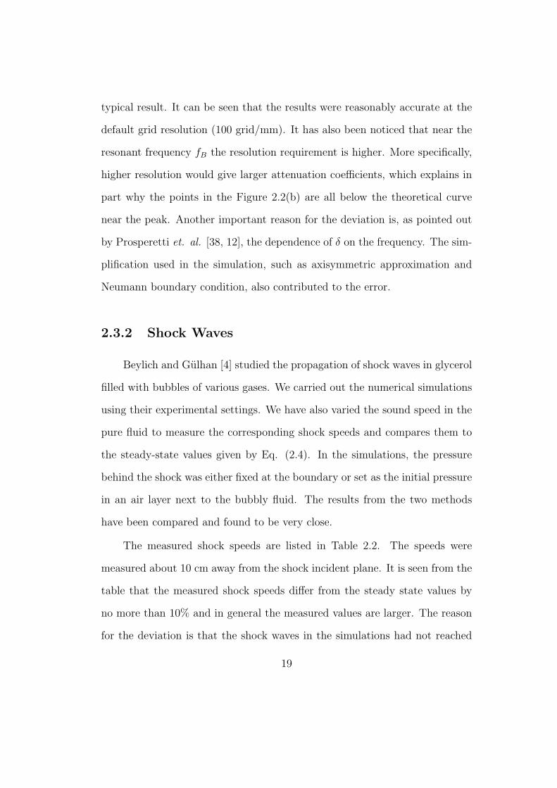
We have also plotted the shock profiles with bubbles of different content
in Figure 2.4. The results were compared to those measured in the experiment
of Beylich et. al. [4]. The profiles were measured at 50 cm away from the
shock incident plane. From the figures we noticed the pressure in the bubbly
fluid oscillates after the passage of the shock front. The oscillation amplitude
was smaller for gas with larger polytropic index γ, which agrees with the
experiment. The period of the oscillation differed from experimental data by
10 to 20 percent, while the amplitude was much smaller in the simulations.
There were several sources of error that could be responsible for the devi-
ation. The main source of error is numerical dissipation at the bubble surface.
The default grid resolution for the simulations on shock wave propagation was
50 grids per centimeter, the bubble radius was also 6-grid wide. It has been
found that increasing resolution did increase the oscillation amplitude but not
drastically. Other sources of error include the axisymmetric approximation
and the Neumann boundary condition on the domain wall. As a summary,
the shock velocity measurement agreed well with the theory, while the shock
profiles agreed with the experiment qualitatively and partly quantitatively.
21
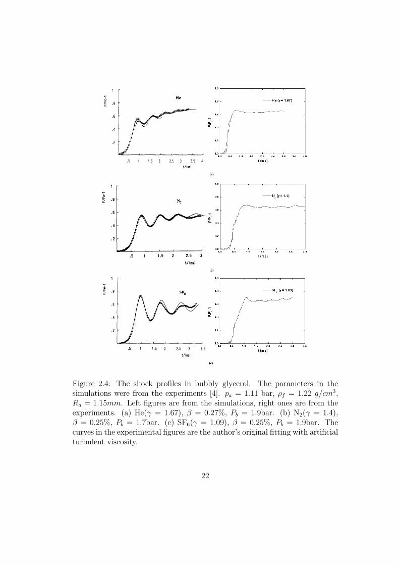
Figure 2.4: The shock profiles in bubbly glycerol. The parameters in thesimulations were from the experiments [4]. pa = 1.11 bar, ρf = 1.22 g/cm3,Ra = 1.15mm. Left figures are from the simulations, right ones are from theexperiments. (a) He(γ = 1.67), β = 0.27%, Pb = 1.9bar. (b) N2(γ = 1.4),β = 0.25%, Pb = 1.7bar. (c) SF6(γ = 1.09), β = 0.25%, Pb = 1.9bar. Thecurves in the experimental figures are the author’s original fitting with artificialturbulent viscosity.
22
Chapter 3
Application of Bubbly Flows to Cavitation
Mitigation
Having validated to some extent the FronTier code for the direct nu-
merical simulation of bubbly flows, we applied it to the cavitation mitigation
problem in the Spallation Neutron Source. In Section 3.1 the design of the SNS
target and associated fluid dynamical issue were described. The description
of the method we used to estimate the collapse pressure of cavitation bubbles
was given in Section 3.2. Section 3.3 listed the results of the simulations using
the front tracking method on the pressure wave propagation in the pure mer-
cury and the mercury injected with non-condensable gas bubbles. In Section
3.4 the collapse pressure of cavitation bubbles was calculated by solving the
Keller equation in the ambient pressure whose profile was obtained from the
simulations. Finally, in Section 3.5 the average collapse pressure with and
without injected bubbles were compared to estimate the cavitation mitigation
efficiency.
23
3.1 Spallation Neutron Source
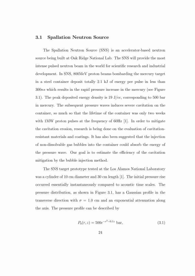
The Spallation Neutron Source (SNS) is an accelerator-based neutron
source being built at Oak Ridge National Lab. The SNS will provide the most
intense pulsed neutron beam in the world for scientific research and industrial
development. In SNS, 800MeV proton beams bombarding the mercury target
in a steel container deposit totally 2.1 kJ of energy per pulse in less than
300ns which results in the rapid pressure increase in the mercury (see Figure
3.1). The peak deposited energy density is 19 J/cc, corresponding to 500 bar
in mercury. The subsequent pressure waves induces severe cavitation on the
container, so much so that the lifetime of the container was only two weeks
with 1MW proton pulses at the frequency of 60Hz [1]. In order to mitigate
the cavitation erosion, research is being done on the evaluation of cavitation-
resistant materials and coatings. It has also been suggested that the injection
of non-dissolvable gas bubbles into the container could absorb the energy of
the pressure wave. Our goal is to estimate the efficiency of the cavitation
mitigation by the bubble injection method.
The SNS target prototype tested at the Los Alamos National Laboratory
was a cylinder of 10 cm diameter and 30 cm length [1]. The initial pressure rise
occurred essentially instantaneously compared to acoustic time scales. The
pressure distribution, as shown in Figure 3.1, has a Gaussian profile in the
transverse direction with σ = 1.0 cm and an exponential attenuation along
the axis. The pressure profile can be described by
P0(r, z) = 500e−r2−0.1z bar, (3.1)
24
Figure 3.1: The pressure distribution right after a pulse of proton beamsin the mercury target of the Spallation Neutron Source. Courtesy of SNSexperimental facilities, Oak Ridge National Lab.
25
where r and z are in cm, and the origin of z axis is the window where proton
beams enter.
3.2 Method of Approach
Before we compare the cavitation erosion in pure and bubbly mercury,
a brief introduction to the mechanism of cavitation damage and the method
we used to quantify it is given in this section. Cavitation is the process in
which a bubble, consisting of vapor and non-condensable gas, expands and
collapses according to the surrounding pressure which decreases and increases
rapidly. Vapor bubbles are formed in the fluid when the pressure falls below
the saturated vapor pressure of the fluid at the ambient temperature. They
implode when the fluid pressure rises back above the saturated vapor pressure
or when the bubbles move into a region with higher pressure. If the bubble is
close to the container wall, the shock wave from the rebound of the collapse
erodes the wall as in the SNS target container.
The attenuation of the pressure wave during the rebound phase of the
cavitation bubbles was studied carefully in [26]. The pressure of the rebounded
wave that hits the container wall is an indicator of the cavitation erosion. Since
it is proportional to the first collapse pressure of cavitation bubbles, for the
estimation of the cavitation mitigation efficiency we only need to compare the
average collapse pressure in the pure mercury and the bubbly mercury. In
order to calculate the collapse pressure, we need to know how the cavitation
bubbles grow and collapse under the pressure wave in the container. Since the
collapsed bubble size (< 0.1µm) is less than a millionth of the container size
26
(10cm), it is difficult to simulate directly the evolution of cavitation bubbles
in the entire container. Instead we did it in two steps.
First, we simulated the propagation of the pressure wave in the container
with the initial distribution given by Eq. (3.1). The simulation was carried
out for both the pure mercury and the mercury injected with non-dissolvable
gas bubbles. For the simulation of the bubbly mercury, the bubble surfaces
were tracked explicitly via the front tracking method that we have described.
The pressure relaxation caused by the cavitation was ignored in the simulation
of pressure waves in the container. We assumed that the growth and collapse
of cavitation bubbles is uncorrelated, namely that the far field liquid pressure
for a cavitation bubble is not significantly perturbed by relaxation waves from
neighboring cavitation bubbles. Since the distribution of cavitation centers is
unknown for mercury under such conditions, accounting for pressure relaxation
processes would contain a large amount of uncertainty.
In the second step, the collapse pressure of cavitation bubbles was cal-
culated by solving the Keller equation (Eq. (2.1)) under the liquid pressure
whose profile was obtained in the first step. A cavitation bubble consists of
vapor and non-condensable gas. The partial pressure of the vapor in the bub-
bles remains negligible compared to the pressure wave in the SNS, while the
partial pressure of the gas (typically air) changes violently. As a result, for
the estimation of the collapse pressure it suffices to calculate the growth and
collapse of the cavitation bubbles that consist of air only.
27
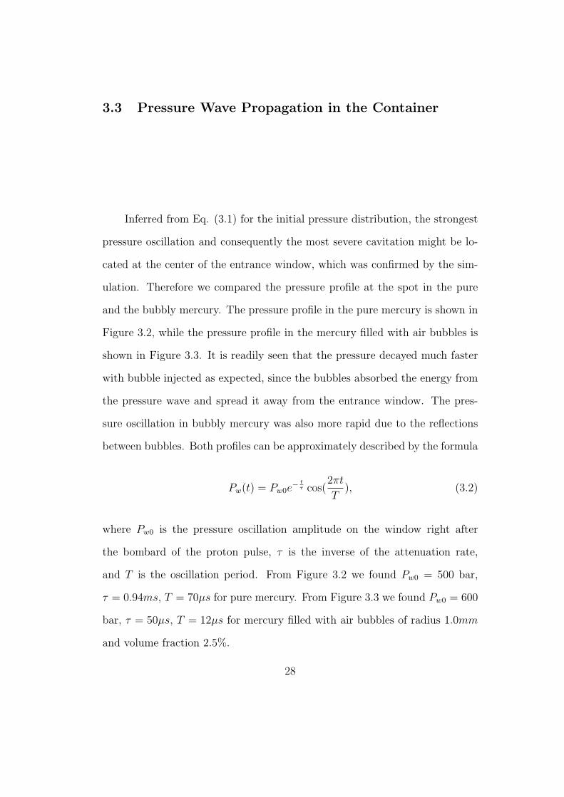
3.3 Pressure Wave Propagation in the Container
Inferred from Eq. (3.1) for the initial pressure distribution, the strongest
pressure oscillation and consequently the most severe cavitation might be lo-
cated at the center of the entrance window, which was confirmed by the sim-
ulation. Therefore we compared the pressure profile at the spot in the pure
and the bubbly mercury. The pressure profile in the pure mercury is shown in
Figure 3.2, while the pressure profile in the mercury filled with air bubbles is
shown in Figure 3.3. It is readily seen that the pressure decayed much faster
with bubble injected as expected, since the bubbles absorbed the energy from
the pressure wave and spread it away from the entrance window. The pres-
sure oscillation in bubbly mercury was also more rapid due to the reflections
between bubbles. Both profiles can be approximately described by the formula
Pw(t) = Pw0e− t
τ cos(2πt
T), (3.2)
where Pw0 is the pressure oscillation amplitude on the window right after
the bombard of the proton pulse, τ is the inverse of the attenuation rate,
and T is the oscillation period. From Figure 3.2 we found Pw0 = 500 bar,
τ = 0.94ms, T = 70µs for pure mercury. From Figure 3.3 we found Pw0 = 600
bar, τ = 50µs, T = 12µs for mercury filled with air bubbles of radius 1.0mm
and volume fraction 2.5%.
28
0 0.2 0.4 0.6 0.8 1 1.2 1.4 1.6 1.8 2−400
−300
−200
−100
0
100
200
300
400
500
t ( ms )
P (
bar
)
Figure 3.2: The pressure profile at the center of the entrance window in thepure mercury.
29
0 0.02 0.04 0.06 0.08 0.1 0.12 0.14 0.16 0.18 0.2−600
−400
−200
0
200
400
600
t ( ms )
P (
bar
)
Figure 3.3: The pressure profile at the center of the entrance window in themercury filled with air bubbles. Bubble radii are 1.0mm and the volumefraction is 2.5%.
30
3.4 Collapse Pressure of Cavitation Bubbles
The second step is the calculation of the collapse pressure of cavitation
bubbles. The Keller equation for the bubble growth and collapse in the weakly
compressible liquid was used for that purpose. With the ambient liquid pres-
sure obtained in the first step, the closed system of equations is
(1− 1
cf
dR
dt)R
d2R
dt2+
3
2(1− 1
3cf
dR
dt)(
dR
dt)2 =
1
ρf
(1 +1
cf
dR
dt+
R
cf
d
dt)(pB − p),
pg = pB +2σ
R,
pgR3 = pg0R
30.
The p in the equation above is the difference between the ambient pressure
and the vapor pressure of mercury in the bubble, however the latter is much
smaller in our case and can be neglected. In the last equation, the gas pressure
in the bubble is associated with the bubble radius by the isothermal relation,
which is valid for the cavitation bubbles in SNS with R0 < 1µm.
To verify that R0 < 1µm for the majority of the cavitation bubbles, recall
that the cavitation bubble grows from a nucleus whose radius is bounded below
by the surface tension condition
2σ
R0
< −p.
For liquid mercury, σ = 0.48kg/s2, in SNS a typical tension of 100 bar gives
R0 > 0.1µm. So it is reasonable to assume the R0 of most cavitation bubbles
are between 0.1µm and 1µm.
31
The pressure waves in both the pure mercury and the bubbly mercury
take on an attenuating sinusoidal form. Since the attenuation is slower than
the oscillation, to obtain the overall collapse pressure of cavitation bubbles we
could calculate it in the purely sinusoidal pressure wave and add it up over the
periods with an attenuating amplitude. The purely sinusoidal pressure wave
has the following form,
p(t) = P sin(2πt
T+ φ0), (3.3)
where φ0 is the initial phase angle when the cavitation bubble starts to grow
from a nucleus. φ0 must be within [-π,0] because for the bubbles to grow
the initial pressure must be below the saturated pressure of mercury, which is
almost 0 compared the the pressure wave in the SNS.
The typical bubble size evolutions with various φ0 are shown in Figure
3.4. It’s interesting to notice that the bubble does not always collapse – the
bubbles beginning to grow at φ0 < −0.8π continues to grow after a period.
Although they may collapse after two or more periods according to the Keller
equation, the associated collapse pressure is smaller since the ambient pressure
has attenuated. On the other hand, for φ0 within [-0.8π,0] the bubble collapses
to a small bubble within about a period. We are only interested in the first
collapse because it has the largest pressure and after that the bubble often
fissures into a cloud of tiny bubbles (cf. [5]) and the Keller equation no longer
applies. Figure 3.5 shows the dependence of the first collapse pressure Pc
on φ0. It is seen that the collapse pressure is highest for φ0 around −0.63π,
32
0 0.25 0.5 0.75 1 1.25 1.50
50
100
150
200
250
t / T
R (
µm
)
φ0 = − 0.9π
φ0 = − 0.7π
φ0 = − 0.5π
φ0 = − 0.3π
φ0 = − 0.1π
Figure 3.4: Bubble size evolution with different φ0. R0 = 1.0µm, pg0 = 0.01bar, P = 100 bar, T = 20µs.
33
−1 −0.9 −0.8 −0.7 −0.6 −0.5 −0.4 −0.3 −0.2 −0.1 00
0.5
1
1.5
2
2.5
3
3.5x 10
12
φ0 / π
Pc (
bar
)P = 300 bar T = 70 µsP = 50 bar T = 70 µsP = 500 bar T = 12 µsP = 50 bar T = 12 µs
Figure 3.5: The first collapse pressure Pc vs. φ0 under the sinusoidal pressurewaves with different amplitude P and period T . The solid line and the dashedline correspond to the pure mercury, the dotted line and the dash-dotted linecorrespond to the mercury filled with air bubbles of radii 1.0mm and volumefraction 2.5%.
and the average collapse pressure Pc is roughly one half of the peak value at
φ0 = −0.63π.
Neglecting the surface tension and the viscosity, which is justified by the
high pressure wave in the liquid, the Keller equation becomes a purely acoustic
equation so that Pc is a function of R0/cfT . On the other hand, so long
as pg0 ¿ |p|, the bubble grows before the first collapse to a maximum size
that depends only on the gas content pg0R30 and the ambient pressure wave.
Therefore Pc is determined by the gas content pg0R30 of the cavitation bubble
34
rather than by R0 and pg0 independently. Combining the two observations,
we see that Pc is a function of P and pg0(R0/cfT )3. In fact, in the range of
P < 10 Kbar and T < 1ms, an empirical formula for Pc with P, T as variables
and pg0, R0 as parameters was obtained,
Pc(P, T ).=
1
2Pc(P, T, φ0 = −0.63π)
.=
93.0
2(
P
ρfc2f
)1.25(pg0
ρfc2f
(R0
cfT)3)−0.50 Kbar, (3.4)
with error less than 1%. The result agreed with the fact that the higher the
rate of stressing the fluid is experiencing, the higher tension can be sustained.
In the bubble injection regime, the period of pressure oscillation T decreases
which in turn reduces the cavitation bubble collapse pressure.
3.5 Efficiency of Cavitation Damage Mitigation
Our goal was to evaluate the mitigation of the cavitation damage by
the bubble injection, i.e. to find the ratio between the overall impact on
the container from the collapses of cavitation bubbles in the pure mercury
and the mercury with non-dissolvable gas bubbles. As mentioned in Section
3.2, we needed only to compare the average collapse pressure Pc. It’s worth
pointing out that, according to Eq. (3.4), Pc can be factored into two parts,
one depending on P and T, and the other one on pg0, R0. This implies that the
ratio between the two cases (with and without bubble injection) is independent
of the size of the initial nucleus and amount of gas in it as long as pg0 ¿ P .
To estimate quantitatively the efficiency of the cavitation mitigation on
35
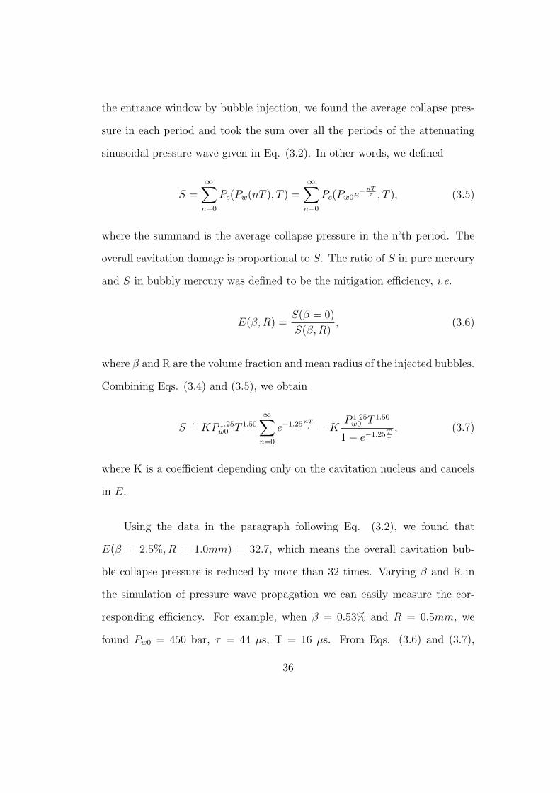
the entrance window by bubble injection, we found the average collapse pres-
sure in each period and took the sum over all the periods of the attenuating
sinusoidal pressure wave given in Eq. (3.2). In other words, we defined
S =∞∑
n=0
Pc(Pw(nT ), T ) =∞∑
n=0
Pc(Pw0e−nT
τ , T ), (3.5)
where the summand is the average collapse pressure in the n’th period. The
overall cavitation damage is proportional to S. The ratio of S in pure mercury
and S in bubbly mercury was defined to be the mitigation efficiency, i.e.
E(β,R) =S(β = 0)
S(β, R), (3.6)
where β and R are the volume fraction and mean radius of the injected bubbles.
Combining Eqs. (3.4) and (3.5), we obtain
S.= KP 1.25
w0 T 1.50
∞∑n=0
e−1.25nTτ = K
P 1.25w0 T 1.50
1− e−1.25Tτ
, (3.7)
where K is a coefficient depending only on the cavitation nucleus and cancels
in E.
Using the data in the paragraph following Eq. (3.2), we found that
E(β = 2.5%, R = 1.0mm) = 32.7, which means the overall cavitation bub-
ble collapse pressure is reduced by more than 32 times. Varying β and R in
the simulation of pressure wave propagation we can easily measure the cor-
responding efficiency. For example, when β = 0.53% and R = 0.5mm, we
found Pw0 = 450 bar, τ = 44 µs, T = 16 µs. From Eqs. (3.6) and (3.7),
36
E(0.53%, 0.5mm) = 42.9.
As a conclusion, we have confirmed the mitigation of cavitation by the
injection of non-dissolvable bubbles. More specifically, we have found that
the injection of bubbles with the volume fraction of order 1% reduces the
cavitation erosion by more than order of magnitude. At the same time, bubbles
absorb/disperse the energy and rapidly attenuate the pressure on the entrance
window of the SNS target so that the cavitation lasts for much shorter time.
37
Chapter 4
Interfacial Dynamics of Phase Transitions
In Section 4.1 the governing equations and boundary conditions are listed.
Section 4.2 gives the alternative forms of the equations. In Section 4.3 and
Section 4.4 we present the analytical solutions to the problem with Riemann
data for the linearized equations with the temperature field decoupled, for
immiscible fluids and phase transitions respectively. In Section 4.5 we explored
the linearized equations with the pressure field decoupled. For both cases, the
solutions to the problem with Riemann data in the two limits κ → 0 and t → 0
are discussed. In Section 4.6 the problem with Riemann data for the nonlinear
equations are solved in both limits. The convergence of the solution to the
classical Riemann solution are analyzed using the method of travelling wave
solutions. Finally the wave structure of the solution are discussed.
4.1 Governing Equations and Boundary Conditions
The governing equations and boundary conditions at the vapor-liquid or
gas-liquid interface are described in detail in [27] and [35]. Away from the in-
38
terface the governing equation is the Navier-Stokes equations for compressible
fluids with body force term. Since the thermal effect is normally dominant
over the viscous effect in bubbly flows [12] and phase transitions [29], viscosity
is neglected in our equations and the numerical algorithm. In the following
equations subscript i = v stands for vapor phase and i = l for liquid phase.
4.1.1 Governing Equations
The conservation equation of mass is
∂ρi
∂t+∇ · (ρiui) = 0, (4.1)
where ρi is the density and ui is the velocity. The conservation equation of
momentum is
∂(ρiui)
∂t+∇ · (ρiuiui) +∇pi = −ρi∇φ, (4.2)
where pi is the pressure, φ the time-independent specific potential of conserv-
ative force, e.g. φ = −g · r for constant gravitational force. The conservation
equation of energy is
∂(ρiEi)
∂t+∇ · ((ρiEi + pi)ui) = −∇ · qi, (4.3)
where Ei is the specific total energy
E =u2
2+ φ + specific internal energy,
39
and qi is the heat flux, which satisfies Fourier’s law of thermal conduction,
q = −κ∇T,
where T is the temperature and κ is the thermal conductivity.
The gas is considered as the ideal gas with γ-law property. The equation
of state for the liquid is of the stiffened polytropic (SPOLY) type, whose
parameters are chosen to fit the thermodynamical quantities at the specific
temperature and pressure. More details are given in Appendix A.
4.1.2 Boundary Conditions at Material Interface
Denote the mass flux across the interface from left to right by M and the
flux from liquid to vapor by Mev. Mev > 0 means evaporation and Mev < 0
means condensation. If the liquid is on the left side then M = Mev, otherwise
M = −Mev. In the following equations subscript n and τ stands for normal
and tangential respectively, ∆ denotes right side minus left side, bar stands
for arithmetic average between the two sides.
The boundary conditions for mass conservation is
∆un = M∆1
ρ= M∆V, (4.4)
where the positive direction of un points from left to right, and V stands for
the specific volume, i.e. the reciprocal of ρ. For the momentum conservation
40
at boundary, Eq. (4.2) should be modified to include the surface tension
∂(ρiui)
∂t+∇ · (ρiuiui) +∇pi +
∫
Γ
psδ(r− rs)nds = −ρi∇φ,
where Γ is the interface and ps is the pressure jump due to surface tension
that equals
ps = σ(κ1 + κ2),
where σ is the surface tension, while κ1 and κ2 are the principal curvatures of
the interface, which are positive when interface is convex toward the positive
n direction. Integrating the equation in an infinitesimally thin slice co-moving
with the interface, we can find the boundary condition for the momentum
conservation to be
∆p + ps + M∆un = 0, (4.5)
M∆uτ = 0, (4.6)
The energy conservation at boundary should also contain the surface energy
as following
∂(ρiEi)
∂t+∇ · ((ρiEi + pi)ui) +
∫
Γ
unpsδ(r− rs)ds = ∇ · (κi∇Ti).
Integrating again, we have the boundary condition for the energy conservation
M(∆H − V ∆p) + ∆qn = 0, (4.7)
41
where H stands for the specific enthalpy
H = specific internal energy + pV.
Due to the thermal conduction, the temperature is continuous across the in-
terface, so
∆T = 0. (4.8)
Thermal contact
If the interface is the contact between two immiscible fluids, then by
definition there is no mass flux across the interface (yet the thermal conduction
is allowed, hence the name ”thermal contact”).
M = 0, (4.9)
so the quantity ∆H − V ∆p on the left side of Eq. (4.7) is arbitrary. The
governing equations combined with the boundary conditions listed above Eqs.
(4.1)–(4.9) are closed. The normal velocity of the two phases are equal at the
contact, and also equal to the normal velocity of the interface.
Uph = un.
The interface is propagated at such velocity in the computation.
42
Phase boundary
In case of phase transitions, M 6= 0 so the value of ∆H − V ∆p plays an
important role in the interfacial dynamics. At equilibrium ∆H is defined as the
latent heat L. In some literatures, e.g. [35], ∆H is fixed to a constant, though
in reality L is not a constant. A better approximation of ∆H is obtained by
linearization near the ambient temperature as in [29], which gives
∆H(T ) = L(Tamb) + (T − Tamb)∆cp(Tamb),
where cp(Tamb) is evaluated at ambient temperature on the phase coexistence
curve. In fact, when the mass flux M is nonzero, the states on both sides of the
phase boundary are not on the phase coexistence curve simultaneously, and so
∆H deviates from the value at equilibrium. Strictly speaking, the value of ∆H
should be calculated from the EOS of the medium. Since our implementation
has complete EOS’s, specifically the SPOLY EOS for the liquid, we can embed
the latent heat into the EOS parameters such that ∆H can be evaluated during
phase transition at the correct pressure and temperature rather than on phase
coexistence curve. The details are given in Appendix A. The correction over
a constant ∆H may be small, but the energy is conserved exactly at least
formally. In practice if the variation of interface temperature is so large that
the latent heat cannot be regarded as a constant or directly embedded into the
EOS parameters, both the latent heat and the phase coexistence curve should
be tabulated and coded into the EOS as extra parameters.
Since the value of M is unknown, we need one more equation to close the
43
system. The kinetic theory of evaporation gives the evaporation rate with a
coefficient determined experimentally. The derivation below follows Alty and
Mackay [3].
Under certain temperature T and pressure p, the molecular velocity of the
vapor, which is treated as ideal gas, has Maxwell distribution. So the number
density
n(u) ∝ exp(− mu2
2kBT),
where m is the molecular mass and kB the Boltzman constant. The total mass
flux of vapor molecules hitting an interface is
m
∫ ∫ ∫
ux>0
duxduyduzn(u)ux
=mN
2ux =
mN
4u =
p√2πRT
,
where N is the total number of molecules per unit volume and R = kB/m.
Not all molecules hitting the phase boundary condense into liquid. The ratio
of molecules condensing into liquid over the total number hitting the phase
boundary is called evaporation coefficient or sometimes condensation coeffi-
cient and denoted by α, which is a number between 0 and 1. Then the mass
flux of the condensing vapor is
αp√
2πRT
at equilibrium. Since the net mass flux cancels at equilibrium, so the mass
flux of evaporating liquid is the same as that of condensing vapor. Denote
44
the equilibrium pressure at temperature T by psat(T ), then the mass flux of
evaporating liquid is
αpsat(T )√2πRT
.
If the temperature is sufficiently lower than the critical temperature of the
material, the rate at which molecules leave the liquid is not affected appreciably
by the presence of surrounding vapor, so that the mass flux of evaporating
liquid is still as above even when the liquid is not at equilibrium with the
vapor. Therefore, the net mass flux of evaporation is
Mev = αpsat(T )− pv√
2πRT. (4.10)
The measurement of α is difficult and values ranges from 0.04 [3] and
below [9, 17] to 0.4 [35] and above [23]. A nice review on the experiments and
theories on the evaporation coefficient can be found in [23].
To implement Eq. (4.10) in the computation we need to know the func-
tion psat(T ), which can be derived from the well-known Clausius-Clapeyron
equation
dP
dT=
∆S
∆V=
L
T (Vv − Vl),
where S stands for specific entropy. Provided the exact EOS for both phases
with latent heat embedded, the phase coexistence curve can be determined
exactly from the EOS’s as the (p, T ) pairs at which the specific Gibbs energy
G = H − TS of both phases equal. In practice, the phase coexistence curve is
often tabulated. For temperature outside the tabulated range, we can extrap-
45
olate the curve by integrating the Clausius-Clapeyron equation with a fixed
L, which gives
psat(T ) = psat(T0) exp(L
Rv
(1
T0
− 1
T)).
Eqs. (4.1)–(4.10) is a closed system of equations. The normal velocity of
two phases are not equal at the phase boundary. An equivalent form of the
boundary condition for mass conservation Eq. (4.4) gives the normal velocity
of the phase boundary,
Uph =∆(ρun)
∆ρ.
The interface is propagated at such velocity in the computation.
4.2 Alternative Forms of the Conservation Laws
4.2.1 Conservation Laws with Rotational Symmetry
When the physical problem has geometrical symmetry it is often more
efficient to reduce the dimension of the system by working in cylindrical or
spherical geometry. The conservation laws Eqs. (4.1)–(4.3) in planar or rota-
tional symmetric coordinates are
∂ρ
∂t+
∂ρu
∂xi
+ αiρu
xi
= 0,
∂ρu
∂t+
∂(ρu2 + p)
∂xi
+ αiρu2
xi
= −ρ∂φ
∂xi
,
∂ρu′
∂t+
∂ρuu′
∂xi
+ αiρuu′
xi
= 0,
∂ρE
∂t+
∂(ρE + p)u
∂xi
+ αi(ρE + p)u
xi
= − ∂q
∂xi
− αiq
xi
, (4.11)
46
where u and u′ are the velocities along xi and perpendicular to xi respectively,
q is the heat flux along xi. αi is the geometrical constant, which is nonzero only
in rotational symmetry and when xi is the first coordinate, i.e. r in cylindrical
or spherical coordinates. In those two cases, α = 1 for cylindrical geometry
while α = 2 for spherical geometry. Please be aware that this geometrical
constant α has nothing to do with the evaporation coefficient in Eq. (4.10),
which is usually also denoted by α.
4.2.2 Conservation Laws on the Interface
The conservation laws projected into the normal direction of the interface
are
∂ρ
∂t+
∂ρu
∂n+ αN0
ρu
r= 0,
∂ρu
∂t+
∂(ρu2 + p)
∂n+ αN0
ρu2
r= −ρ
∂φ
∂n,
∂ρu′
∂t+
∂ρuu′
∂n+ αN0
ρuu′
r= 0,
∂ρE
∂t+
∂(ρE + p)u
∂n+ αN0
(ρE + p)u
r= − ∂q
∂n− αN0
q
r,
where n is the normal direction of the interface, u and u′ the normal and
tangential velocity respectively, q is the normal heat flux. N0 is the x compo-
nent of the n. ∂∂n
is the directional derivative in the direction n. The above
equations are similar to those given in [21] except for the thermal conduction
47
terms. The noncharacteristic version of the above equations is
Dρ
Dt+ ρ(
∂u
∂n+ αN0
u
r) = 0,
Du
Dt+
1
ρ
∂p
∂n= −∂φ
∂n,
Du′
Dt= 0,
De
Dt+ p
DV
Dt= −1
ρ(∂q
∂n+ αN0
q
r),
where e and V are the specific internal energy and specific volume, while DDt
is the Lagrangian derivative
D
Dt=
∂
∂t+ u
∂
∂n.
A convenient form of the conservation laws at the interface for numerical
algorithms is the characteristic form.
dp
dλ+
+ αN0ρc2u
r+ ρc
du
dλ+
= −ρc∂φ
∂n− Γ(
∂q
∂n+ αN0
q
r), (4.12)
dp
dλ−+ αN0
ρc2u
r− ρc
du
dλ−= ρc
∂φ
∂n− Γ(
∂q
∂n+ αN0
q
r), (4.13)
du′
dλ0
= 0, (4.14)
de
dλ0
+ pdV
dλ0
= −1
ρ(∂q
∂n+ αN0
q
r). (4.15)
where
c =
√(∂p
∂ρ
)
S
is the sound speed and S is the specific entropy. Γ is the Gruneisen coefficient
48
[36]
Γ = V
(∂p
∂e
)
V
=V
T
(∂p
∂S
)
V
.
For both POLY and SPOLY EOS’s, Γ = γ−1, where γ is the polytropic index.
The characteristic derivatives λ± and λ0 are defined by
d
dλ±=
∂
∂t+ (u± c)
∂
∂n,
d
dλ0
=∂
∂t+ u
∂
∂n. (4.16)
Notice the important difference in the characteristic equations that the entropy
S is no longer conserved.
From the second law of thermodynamics, TdS = de + pdV , Eqs. (4.12)
and (4.13) can be verified as following,
dp
dλ±+ αN0
ρc2u
r± ρc
du
dλ±
=Dp
Dt± c
∂p
∂n+ αN0
ρc2u
r± ρc(
Du
Dt± c
∂u
∂n)
=Dp
Dt+ ρc2(
∂u
∂n+ αN0
u
r)± c(ρ
Du
Dt+
∂p
∂n)
=Dp
Dt− c2 Dρ
Dt∓ ρc
∂φ
∂n
=Dp
Dt−
(∂p
∂ρ
)
S
Dρ
Dt∓ ρc
∂φ
∂n
=
(∂p
∂S
)
ρ
DS
Dt∓ ρc
∂φ
∂n
= −(
∂p
∂S
)
V
· V
T(∂q
∂n+ αN0
q
r)∓ ρc
∂φ
∂n
= −Γ(∂q
∂n+ αN0
q
r)∓ ρc
∂φ
∂n.
49
An equivalent form of Eq. (4.15) is
−(∂q
∂n+ αN0
q
r) = ρ(
de
dλ0
+ pdV
dλ0
)
= ρDH
Dt− Dp
Dt
= ρcpDT
Dt+ (ρ
(∂H
∂p
)
T
− 1)Dp
Dt
= ρcpDT
Dt− βT
Dp
Dt, (4.17)
where β is the coefficient of thermal expansion [36],
β =1
V
(∂V
∂T
)
p
.
For ideal gas βT ≡ 1. For liquid, e.g. water in room temperature, βT ¿ 1.
If the heat flux satisfies Fourier’s law of thermal conduction, i.e. q =
−κ∇T , then the Eqs. (4.12)–(4.15) is a parabolic system. The problem with
Riemann data does not have the classical self-similar solution.
To have a flavor of the solution, let us investigate the linearized equations
without gravity in one-dimensional planar geometry. For clarity the equations
are listed below, in which Eq. (4.17) has been substituted for Eq. (4.15).
∂(p + mu)
∂t+ c
∂(p + mu)
∂x= Γκ
∂2T
∂x2,
∂(p−mu)
∂t− c
∂(p−mu)
∂x= Γκ
∂2T
∂x2,
ρcp∂T
∂t− βT
∂p
∂t= κ
∂2T
∂x2,
where m = ρc and all other coefficients c, κ, Γ, ρcp and βT are taken to be
50
constants. If βT 6= 0 and Γ 6= 0, the equations above are coupled and hard to
solve analytically. On the other hand, if βT is neglected, which is justified for
most liquids, the system is decoupled. We can solve the temperature equation
analytically and substitute the solution for the right-hand-side of the other two
equations. In this case the parabolic (temperature) field revises the hyperbolic
(pressure and velocity) fields. On the other hand, if Γ is taken to be zero, then
the pressure and velocity can be solved directly and substituted for the ∂p∂t
term
in the thermal equation. Here the hyperbolic fields revise the parabolic field. If
neither βT nor Γ vanishes, the two types of fields closely interact. Closed form
solution hasn’t been derived even for linearized equations. However, from the
observation on the solution in the two special cases mentioned above, aspects
of the solution in certain limits can be derived. The following is the detail.
4.3 Analytical Solution for Immiscible Fluids: Temper-
ature Field Decoupled
First let us consider the case that βT vanishes. The temperature field
is decoupled from the hyperbolic fields, and the isentropes coincide with the
isotherms. Since the thermal contact is simpler than phase boundary, we will
begin with thermal contact. Assume the two phases to the left and right of
the origin satisfy the linearized equations with different coefficients, and the
Cauchy data in each phase is constant as in the Riemann problem. More
51
clearly,
∂(pl + mlul)
∂t+ cl
∂(pl + mlul)
∂x= Γlκl
∂2Tl
∂x2, (4.18)
∂(pl −mlul)
∂t− cl
∂(pl −mlul)
∂x= Γlκl
∂2Tl
∂x2, (4.19)
(ρcp)l∂Tl
∂t= κl
∂2Tl
∂x2, (4.20)
∂(pr + mrur)
∂t+ cr
∂(pr + mrur)
∂x= Γrκr
∂2Tr
∂x2, (4.21)
∂(pr −mrur)
∂t− cr
∂(pr −mrur)
∂x= Γrκr
∂2Tr
∂x2, (4.22)
(ρcp)r∂Tr
∂t= κr
∂2Tr
∂x2, (4.23)
with Cauchy data
(pl, ul, Tl)(t = 0) = (pl0, ul0, Tl0)
(pr, ur, Tr)(t = 0) = (pr0, ur0, Tr0).
The condition at the interface is
pl(x = 0) = pr(x = 0) (4.24)
ul(x = 0) = ur(x = 0) (4.25)
Tl(x = 0) = Tr(x = 0) (4.26)
κl
(∂Tl
∂x
)
x=0
= κr
(∂Tr
∂x
)
x=0
. (4.27)
52
4.3.1 Analytical Solution
Temperature
From Eqs. (4.20), (4.23), (4.26), (4.27) and the Cauchy data we can derive
the analytical solution for the temperature field.
Tl(t, x) = Tm − (Tl0 − Tm)erf(x√4νlt
), (4.28)
Tr(t, x) = Tm + (Tr0 − Tm)erf(x√4νrt
), (4.29)
where
Tm =Tl0
√(ρcpκ)l + Tr0
√(ρcpκ)r√
(ρcpκ)l +√
(ρcpκ)r
, (4.30)
and ν = κ/(ρcp). Erf is the error function defined as
erf(x) =2√π
∫ x
0
e−y2
dy.
From Eqs. (4.28) and (4.29) we know
∂2Tl
∂x2(t, x) = (Tl0 − Tm)
x
νlt√
4πνlte− x2
4νlt ,
∂2Tr
∂x2(t, x) = −(Tr0 − Tm)
x
νrt√
4πνrte−
x2
4νrt .
53
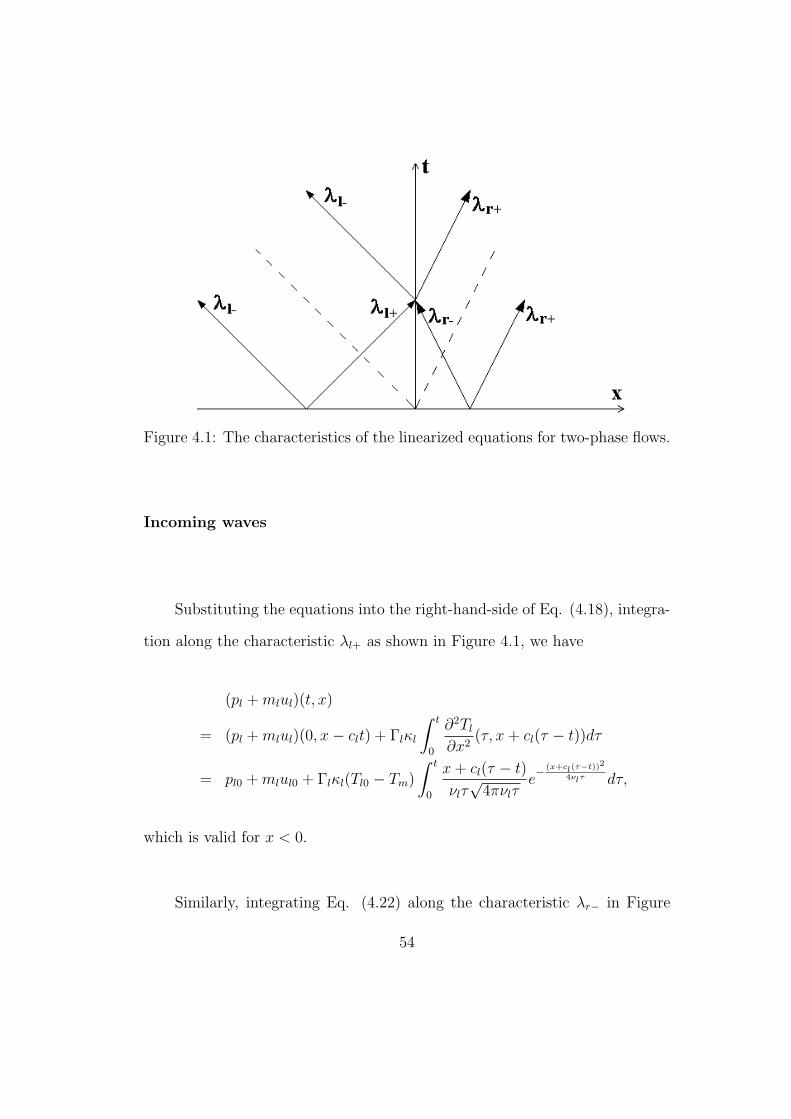
Figure 4.1: The characteristics of the linearized equations for two-phase flows.
Incoming waves
Substituting the equations into the right-hand-side of Eq. (4.18), integra-
tion along the characteristic λl+ as shown in Figure 4.1, we have
(pl + mlul)(t, x)
= (pl + mlul)(0, x− clt) + Γlκl
∫ t
0
∂2Tl
∂x2(τ, x + cl(τ − t))dτ
= pl0 + mlul0 + Γlκl(Tl0 − Tm)
∫ t
0
x + cl(τ − t)
νlτ√
4πνlτe− (x+cl(τ−t))2
4νlτ dτ,
which is valid for x < 0.
Similarly, integrating Eq. (4.22) along the characteristic λr− in Figure
54
4.1, we have
(pr −mrur)(t, x)
= (pr −mrur)(0, x + crt) + Γrκr
∫ t
0
∂2Tr
∂x2(τ, x− cr(τ − t))dτ
= pr0 −mrur0 − Γrκr(Tr0 − Tm)
∫ t
0
x− cr(τ − t)
νrτ√
4πνrτe−
(x−cr(τ−t))2
4νrτ dτ,
which is valid for x > 0.
Outgoing waves
For points below the left dashed line in Figure 4.1, i.e. x < −clt, we can
integrate Eq. (4.19) along the characteristic λl− to obtain
(pl −mlul)(t, x)
= (pl −mlul)(0, x + clt) + Γlκl
∫ t
0
∂2Tl
∂x2(τ, x− cl(τ − t))dτ
= pl0 −mlul0 + Γlκl(Tl0 − Tm)
∫ t
0
x− cl(τ − t)
νlτ√
4πνlτe− (x−cl(τ−t))2
4νlτ dτ.
On the other hand, for points in the left half space and above the left dashed
line, i.e. −clt < x < 0, we need to integrate from the interface, where the
state is determined by the information coming along characteristics λl+ and
λr− and boundary conditions Eqs. (4.24) and (4.25). At the interface x = 0,
p(t, 0) =mr(pl + mlul)(t, 0) + ml(pr −mrur)(t, 0)
mr + ml
,
u(t, 0) =(pl + mlul)(t, 0)− (pr −mrur)(t, 0)
mr + ml
.
55
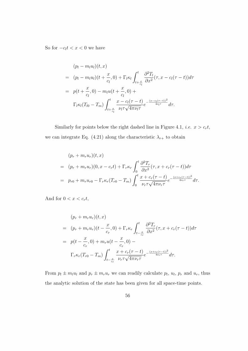
So for −clt < x < 0 we have
(pl −mlul)(t, x)
= (pl −mlul)(t +x
cl
, 0) + Γlκl
∫ t
t+ xcl
∂2Tl
∂x2(τ, x− cl(τ − t))dτ
= p(t +x
cl
, 0)−mlu(t +x
cl
, 0) +
Γlκl(Tl0 − Tm)
∫ t
t+ xcl
x− cl(τ − t)
νlτ√
4πνlτe− (x−cl(τ−t))2
4νlτ dτ.
Similarly for points below the right dashed line in Figure 4.1, i.e. x > crt,
we can integrate Eq. (4.21) along the characteristic λr+ to obtain
(pr + mrur)(t, x)
= (pr + mrur)(0, x− crt) + Γrκr
∫ t
0
∂2Tr
∂x2(τ, x + cr(τ − t))dτ
= pr0 + mrur0 − Γrκr(Tr0 − Tm)
∫ t
0
x + cr(τ − t)
νrτ√
4πνrτe−
(x+cr(τ−t))2
4νrτ dτ.
And for 0 < x < crt,
(pr + mrur)(t, x)
= (pr + mrur)(t− x
cr
, 0) + Γrκr
∫ t
t− xcr
∂2Tr
∂x2(τ, x + cr(τ − t))dτ
= p(t− x
cr
, 0) + mru(t− x
cr
, 0)−
Γrκr(Tr0 − Tm)
∫ t
t− xcr
x + cr(τ − t)
νrτ√
4πνrτe−
(x+cr(τ−t))2
4νrτ dτ.
From pl ±mlul and pr ±mrur we can readily calculate pl, ul, pr and ur, thus
the analytic solution of the state has been given for all space-time points.
56
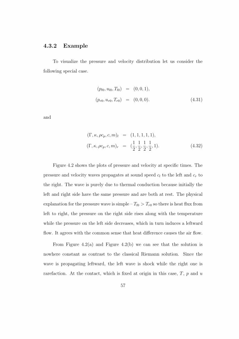
4.3.2 Example
To visualize the pressure and velocity distribution let us consider the
following special case.
(pl0, ul0, Tl0) = (0, 0, 1),
(pr0, ur0, Tr0) = (0, 0, 0). (4.31)
and
(Γ, κ, ρcp, c,m)l = (1, 1, 1, 1, 1),
(Γ, κ, ρcp, c, m)r = (1
2,1
2,1
2,1
2, 1). (4.32)
Figure 4.2 shows the plots of pressure and velocity at specific times. The
pressure and velocity waves propagates at sound speed cl to the left and cr to
the right. The wave is purely due to thermal conduction because initially the
left and right side have the same pressure and are both at rest. The physical
explanation for the pressure wave is simple – Tl0 > Tr0 so there is heat flux from
left to right, the pressure on the right side rises along with the temperature
while the pressure on the left side decreases, which in turn induces a leftward
flow. It agrees with the common sense that heat difference causes the air flow.
From Figure 4.2(a) and Figure 4.2(b) we can see that the solution is
nowhere constant as contrast to the classical Riemann solution. Since the
wave is propagating leftward, the left wave is shock while the right one is
rarefaction. At the contact, which is fixed at origin in this case, T , p and u
57
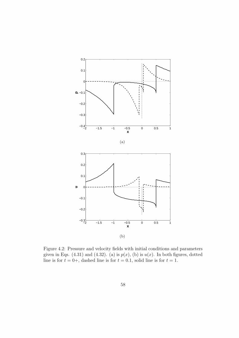
−2 −1.5 −1 −0.5 0 0.5 1−0.4
−0.3
−0.2
−0.1
0
0.1
0.2
p
x
(a)
−2 −1.5 −1 −0.5 0 0.5 1−0.3
−0.2
−0.1
0
0.1
0.2
0.3
u
x
(b)
Figure 4.2: Pressure and velocity fields with initial conditions and parametersgiven in Eqs. (4.31) and (4.32). (a) is p(x), (b) is u(x). In both figures, dottedline is for t = 0+, dashed line is for t = 0.1, solid line is for t = 1.
58
are all conserved, though density and energy can have discontinuity as usual.
The ”mid state” is varying with both time and space, so it is not well-defined
in the classical sense. However, we can investigate two limit cases, namely,
t →∞ and t → 0.
4.3.3 Asymptotic Solution in the Adiabatic Limit
First let us consider the case that t → ∞. By scaling the conservation
laws, it is easy to see that the limit κ → 0 is equivalent to the limit that t →∞and x → ∞ simultaneously while keeping x/t unchanged. Therefore this is
the limit of vanishing thermal conductivity, in other words, the adiabatic limit.
We might expect the problem to be reduced to the classical Riemann problem
in this limit, however it is not quite true due to the condition of temperature
continuity that is absent in the classical Riemann problem. Figure 4.3 shows
the plots of pressure and velocity with decreasing thermal conductivity κ. It
is seen that the amplitude of the pressure and velocity wave does not vanish in
the limit of κ → 0, yet the width of the pressure and velocity peak approaches
0. Next we will prove it rigorously and derive the limit peak values of the
pressure and velocity waves.
Thermal effect
The effect of the thermal conduction can be understood as a linear su-
perposition onto the classical Riemann solution. If the thermal conduction
is absent, then the characteristics λl+ and λr− intersect at the interface and
determine the mid state and thus the global piecewise constant solution struc-
59
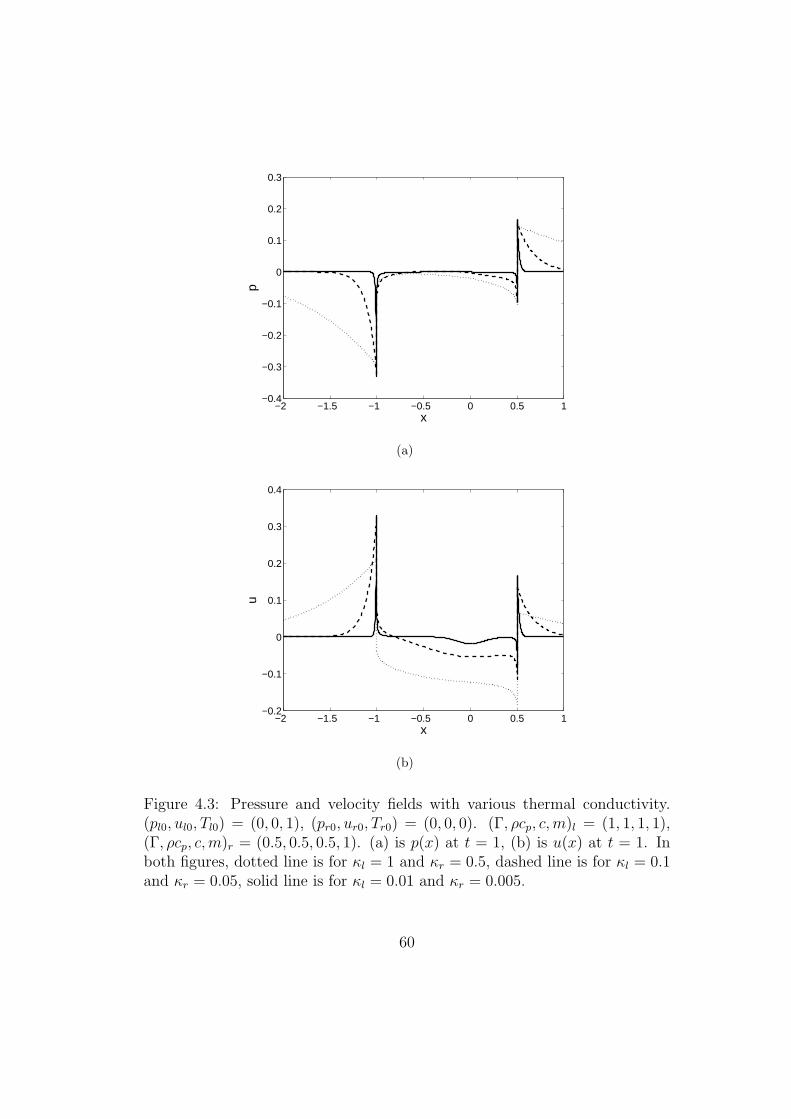
−2 −1.5 −1 −0.5 0 0.5 1−0.4
−0.3
−0.2
−0.1
0
0.1
0.2
0.3
x
p
(a)
−2 −1.5 −1 −0.5 0 0.5 1−0.2
−0.1
0
0.1
0.2
0.3
0.4
x
u
(b)
Figure 4.3: Pressure and velocity fields with various thermal conductivity.(pl0, ul0, Tl0) = (0, 0, 1), (pr0, ur0, Tr0) = (0, 0, 0). (Γ, ρcp, c, m)l = (1, 1, 1, 1),(Γ, ρcp, c, m)r = (0.5, 0.5, 0.5, 1). (a) is p(x) at t = 1, (b) is u(x) at t = 1. Inboth figures, dotted line is for κl = 1 and κr = 0.5, dashed line is for κl = 0.1and κr = 0.05, solid line is for κl = 0.01 and κr = 0.005.
60
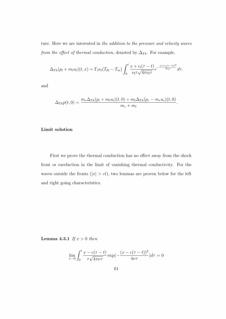
ture. Here we are interested in the addition to the pressure and velocity waves
from the effect of thermal conduction, denoted by ∆Th. For example,
∆Th(pl + mlul)(t, x) = Γlκl(Tl0 − Tm)
∫ t
0
x + cl(τ − t)
νlτ√
4πνlτe− (x+cl(τ−t))2
4νlτ dτ.
and
∆Thp(t, 0) =mr∆Th(pl + mlul)(t, 0) + ml∆Th(pr −mrur)(t, 0)
mr + ml
.
Limit solution
First we prove the thermal conduction has no effect away from the shock
front or rarefaction in the limit of vanishing thermal conductivity. For the
waves outside the fronts (|x| > ct), two lemmas are proven below for the left
and right going characteristics.
Lemma 4.3.1 If x > 0 then
limν→0
∫ t
0
x− c(τ − t)
τ√
4πντexp(−(x− c(τ − t))2
4ντ)dτ = 0
61
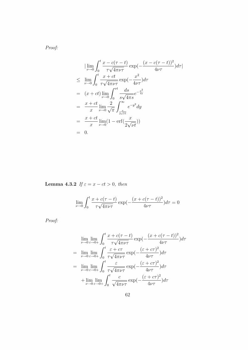
Proof:
| limν→0
∫ t
0
x− c(τ − t)
τ√
4πντexp(−(x− c(τ − t))2
4ντ)dτ |
≤ limν→0
∫ t
0
x + ct
τ√
4πντexp(− x2
4ντ)dτ
= (x + ct) limν→0
∫ νt
0
ds
s√
4πse−
x2
4s
=x + ct
xlimν→0
2√π
∫ ∞
x2√
νt
e−y2
dy
=x + ct
xlimν→0
(1− erf(x
2√
νt))
= 0.
Lemma 4.3.2 If ε = x− ct > 0, then
limν→0
∫ t
0
x + c(τ − t)
τ√
4πντexp(−(x + c(τ − t))2
4ντ)dτ = 0
Proof:
limν→0
limε→0+
∫ t
0
x + c(τ − t)
τ√
4πντexp(−(x + c(τ − t))2
4ντ)dτ
= limν→0
limε→0+
∫ t
0
ε + cτ
τ√
4πντexp(−(ε + cτ)2
4ντ)dτ
= limν→0
limε→0+
∫ t
0
ε
τ√
4πντexp(−(ε + cτ)2
4ντ)dτ
+ limν→0
limε→0+
∫ t
0
c√4πντ
exp(−(ε + cτ)2
4ντ)dτ
62
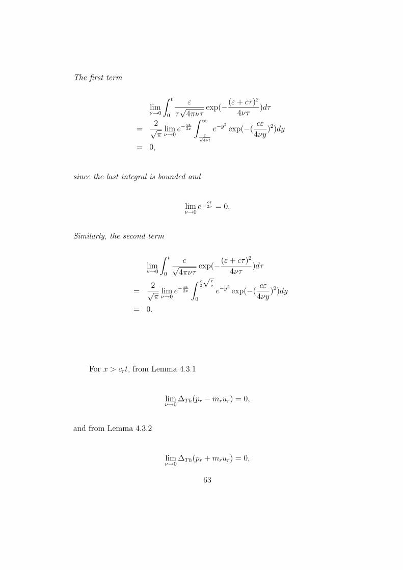
The first term
limν→0
∫ t
0
ε
τ√
4πντexp(−(ε + cτ)2
4ντ)dτ
=2√π
limν→0
e−cε2ν
∫ ∞
ε√4νt
e−y2
exp(−(cε
4νy)2)dy
= 0,
since the last integral is bounded and
limν→0
e−cε2ν = 0.
Similarly, the second term
limν→0
∫ t
0
c√4πντ
exp(−(ε + cτ)2
4ντ)dτ
=2√π
limν→0
e−cε2ν
∫ c2
√tν
0
e−y2
exp(−(cε
4νy)2)dy
= 0.
For x > crt, from Lemma 4.3.1
limν→0
∆Th(pr −mrur) = 0,
and from Lemma 4.3.2
limν→0
∆Th(pr + mrur) = 0,
63
so limν→0 ∆Th(pr) = 0 and limν→0 ∆Th(ur) = 0. The case of x < clt is similar.
For the waves inside the fronts (|x| < ct), two more lemmas are needed.
Lemma 4.3.3 For x = 0,
limt→∞
∫ t
0
x− c(τ − t)
τ√
4πντexp(−(x− c(τ − t))2
4ντ)dτ = 0
Proof:
limt→∞
∫ t
0
x− c(τ − t)
τ√
4πντexp(−(x− c(τ − t))2
4ντ)dτ
= limt→∞
∫ t
0
c(t− τ)
τ√
4πντexp(−c2(t− τ)2
4ντ)dτ
=2√π
limt→∞
∫ ∞
c2
√tν
(1− c2t
4νy2) exp(−y2(1− c2t
4νy2)2)dy
=2√π
limα= c
2
√tν→∞
∫ ∞
α
(1− (α
y)2) exp(−y2(1− (
α
y)2)2)dy
= limα→∞
2√π
∫ α+ 3√α
α
(1− (α
y)2) exp(−y2(1− (
α
y)2)2)dy
+ limα→∞
2√π
∫ ∞
α+ 3√α
(1− (α
y)2) exp(−y2(1− (
α
y)2)2)dy
≤ 2√π
limα→∞
[
∫ α+ 3√α
α
(1− (α
α + 3√
α)2)dy +
∫ ∞
α+ 3√α
exp(−(y − α2
α + 3√
α)2)dy]
≤ limα→∞
[2√π
23√
α+ 1− erf( 3
√α)]
= 0.
Lemma 4.3.4 If 0 < x < ct, then
limν→0
∫ t
t−xc
x + c(τ − t)
τ√
4πντexp(−(x + c(τ − t))2
4ντ)dτ = 0
64
Proof: Denote ε = ct− x, we have
limν→0
∫ t
t−xc
x + c(τ − t)
τ√
4πντexp(−(x + c(τ − t))2
4ντ)dτ
=2√π
limν→0
∫ 12
√cxν
0
dy(1 +εc
4νy2)−
32 exp(− y2
1 + εc4νy2
).
Obviously it is nonnegative. Since y ≤ 12
√cxν, 1 + εc
4νy2 ≤ εc4νy2 (1 + x
ε), and so
2√π
limν→0
∫ 12
√cxν
0
dy(1 +εc
4νy2)−
32 exp(− y2
1 + εc4νy2
).
≤ 2√π
limν→0
∫ 12
√cxν
0
dy(εc
4νy2)−
32 exp(− y2
εc4νy2 (1 + x
ε)).
= limν→0
ε + x
ε
√ν
πεc(1− exp(− c
4ν
x2
ε + x))
= 0.
For 0 < x < crt, first applying Lemma 4.3.3 on both sides (along λl+
and λr−) we see limν→0 ∆Th(pbd) = 0 and limν→0 ∆Th(ubd) = 0, where pbd and
ubd stand for the pressure and velocity on the interface. Then from Lemma
4.3.1 and Lemma 4.3.4 we draw the same conclusion as for x > crt. The
case of −clt < x < 0 is similar. As a summary, away from the shock front
or rarefaction, the thermal conduction has no effect in the limit of vanishing
thermal conductivity. However it is not so at the front. Again we consider
waves outside the fronts first.
65
Lemma 4.3.5 If x = ct then
limν→0
∫ t
0
x + c(τ − t)
τ√
4πντexp(−(x + c(τ − t))2
4ντ)dτ = 1
Proof:
limν→0
∫ t
0
x + c(τ − t)
τ√
4πντexp(−(x + c(τ − t))2
4ντ)dτ
= limν→0
∫ t
0
c√4πντ
e−c2
4ντdτ
=2√π
limν→0
∫ c2
√tν
0
e−y2
dy
= limν→0
erf(c
2
√t
ν)
= 1.
Lemma 4.3.6 Define ε = x− ct, then
limν→0
limε→0+
∫ t
0
x + c(τ − t)
τ√
4πντexp(−(x + c(τ − t))2
4ντ)dτ = 2
Proof: As the proof of Lemma 4.3.2, the integral can be written as the sum of
66
two terms. Now the first term
limν→0
limε→0+
∫ t
0
ε
τ√
4πντexp(−(ε + cτ)2
4ντ)dτ
=2√π
limν→0
limε→0+
∫ ∞
ε√4νt
exp(−(y +cε
4νy)2)dy
=2√π
limν→0
limε→0+
e−cε2ν
∫ ∞
ε√4νt
e−y2
exp(−(cε
4νy)2)dy
=2√π
limν→0
limε→0+
∫ ∞
ε√4νt
e−y2
exp(−(cε
4νy)2)dy.
It is bounded from above by erf(∞) = 1. We can show it is also bounded from
below by 1. Indeed,
2√π
limν→0
limε→0+
∫ ∞
ε√4νt
e−y2
exp(−(cε
4νy)2)dy.
≥ 2√π
limν→0
limε→0+
∫ ∞
max( ε√4νt
,√
cε4ν
)
e−y2
exp(−(cε
4νy)2)dy
≥ 2√π
limν→0
limε→0+
e−cε4ν
∫ ∞
max( ε√4νt
,√
cε4ν
)
e−y2
dy
= limν→0
limε→0+
e−cε4ν (1− erf(max(
ε√4νt
,
√cε
4ν))
= 1.
Comparing the second term with Lemma 4.3.5 we can see that it is bounded
67
from above by 1. Similarly it is also bounded from below by 1. Indeed,
limν→0
limε→0+
∫ t
0
c√4πντ
exp(−(ε + cτ)2
4ντ)dτ
=2√π
limν→0
limε→0+
∫ c2
√tν
0
exp(−(y +cε
4νy)2)dy
=2√π
limν→0
limε→0+
e−cε2ν
∫ c2
√tν
0
e−y2
exp(−(cε
4νy)2)dy
≥ 2√π
limν→0
limε→0+
∫ c2
√tν
√cε4ν
e−y2
exp(−(cε
4νy)2)dy
≥ 2√π
limν→0
limε→0+
e−cε4ν
∫ c2
√tν
√cε4ν
e−y2
dy
= limν→0
limε→0+
e−cε4ν (erf(
c
2
√t
ν)− erf(
√cε
4ν))
= 1.
First let x− crt → 0+ for the right wave. Lemma 4.3.1 gives
limν→0
limx−crt→0+
∆Th(pr −mrur) = 0
as before. Yet Lemma 4.3.6 gives
limν→0
limx−crt→0+
∆Th(pr + mrur) = 2Γr(ρcp)r(Tm − Tr0).
68
Therefore
limν→0
limx−crt→0+
∆Thpr = Γr(ρcp)r(Tm − Tr0)
= Γr(ρcp)r(Tl0 − Tr0)
√(ρcpκ)l√
(ρcpκ)l +√
(ρcpκ)r
limν→0
limx−crt→0+
∆Thur =1
mr
Γr(ρcp)r(Tm − Tr0)
=1
mr
Γr(ρcp)r(Tl0 − Tr0)
√(ρcpκ)l√
(ρcpκ)l +√
(ρcpκ)r
.
Similarly for the left wave,
limν→0
limx+clt→0−
∆Thpl = Γl(ρcp)l(Tr0 − Tl0)
√(ρcpκ)r√
(ρcpκ)l +√
(ρcpκ)r
limν→0
limx+clt→0−
∆Thul = − 1
ml
Γl(ρcp)l(Tr0 − Tl0)
√(ρcpκ)r√
(ρcpκ)l +√
(ρcpκ)r
,
For the height of waves inside the fronts, two more lemmas are needed.
Lemma 4.3.7 For 0 < x < ct, denote ε = ct− x, we have
limν→0
limε→0+
∫ t
t−xc
x + c(τ − t)
τ√
4πντexp(−(x + c(τ − t))2
4ντ)dτ = 1
69
Proof: Denote ε = ct− x, we have
limν→0
limε→0+
∫ t
t−xc
x + c(τ − t)
τ√
4πντexp(−(x + c(τ − t))2
4ντ)dτ
=2√π
limν→0
limε→0+
∫ 12
√cxν
0
dy(1 +εc
4νy2)−
32 exp(− y2
1 + εc4νy2
)
=2√π
limν→0
limε→0+
∫ 3√
εc4ν
0
dy(1 +εc
4νy2)−
32 exp(− y2
1 + εc4νy2
)
+2√π
limν→0
limε→0+
∫ 12
√cxν
3√
εc4ν
dy(1 +εc
4νy2)−
32 exp(− y2
1 + εc4νy2
).
The first term vanishes since the integral domain width vanishes in the limit
ε → 0. In the second term
ε
x≤ εc
4νy2≤ 3
√εc
4ν,
so the second term equals
2√π
limν→0
limε→0+
∫ 12
√cxν
3√
εc4ν
dye−y2
= 1.
Lemma 4.3.8 For x = 0,
limt→0
∫ t
0
x− c(τ − t)
τ√
4πντexp(−(x− c(τ − t))2
4ντ)dτ = 1
70
Proof:
limt→0
∫ t
0
x− c(τ − t)
τ√
4πντexp(−(x− c(τ − t))2
4ντ)dτ
=2√π
limα= c
2
√tν→0
∫ ∞
α
(1− (α
y)2) exp(−y2(1− (
α
y)2)2)dy.
As we have done several times the domain of the integral can be divided into
two subdomains, namely, [α,√
α] and [√
α,∞). The integral in the first sub-
domain vanishes in the limit of α → 0, while the one in the second subdomain
approaches limα→0 1− erf(α) = 1 since (αy)2 < α in the subdomain.
Note: In this lemma, the limit is taken at t → 0 unlike the limit of ν → 0
in all previous lemmas.
Let x − crt → 0− for the right wave. Lemma 4.3.8 applied on the right
side along λr− gives
limt→0
∆Th(pr −mrur)(t, 0) = Γr(ρcp)r(Tm − Tr0),
and applied on the left side along λl+ gives
limt→0
∆Th(pl + mlul)(t, 0) = Γl(ρcp)l(Tm − Tl0).
So
limt→0
∆Thp(t, 0) =mrΓl(ρcp)l(Tm − Tl0) + mlΓr(ρcp)r(Tm − Tr0)
mr + ml
,
and
limt→0
∆Thu(t, 0) =Γl(ρcp)l(Tm − Tl0)− Γr(ρcp)r(Tm − Tr0)
mr + ml
.
71
Applying Lemma 4.3.7 we have
limν→0
limx−crt→0−
∆Th(pr + mrur)
= limν→0
[limt→0
∆Thp(t, 0) + mr limt→0
∆Thu(t, 0)] + Γr(ρcp)r(Tm − Tr0)
=mrΓl(ρcp)l(Tm − Tl0) + mlΓr(ρcp)r(Tm − Tr0)
mr + ml
+mrΓl(ρcp)l(Tm − Tl0)− Γr(ρcp)r(Tm − Tr0)
mr + ml
+ Γr(ρcp)r(Tm − Tr0)
= 2mrΓl(ρcp)l(Tm − Tl0) + mlΓr(ρcp)r(Tm − Tr0)
mr + ml
.
Using Lemma 4.3.1 again we have
limν→0
limx→crt−
∆Thpr =mrΓl(ρcp)l(Tm − Tl0) + mlΓr(ρcp)r(Tm − Tr0)
mr + ml
=Tr0 − Tl0
mr + ml
Γl(ρcp)lmr
√(ρcpκ)r − Γr(ρcp)rml
√(ρcpκ)l√
(ρcpκ)l +√
(ρcpκ)r
limν→0
limx→crt−
∆Thur =Tr0 − Tl0
mr(mr + ml)
Γl(ρcp)lmr
√(ρcpκ)r − Γr(ρcp)rml
√(ρcpκ)l√
(ρcpκ)l +√
(ρcpκ)r
.
Similarly for the left wave inside the front,
limν→0
limx→−clt+
∆Thpl = limν→0
limx→crt−
∆Thpr
=Tr0 − Tl0
mr + ml
Γl(ρcp)lmr
√(ρcpκ)r − Γr(ρcp)rml
√(ρcpκ)l√
(ρcpκ)l +√
(ρcpκ)r
limν→0
limx→−clt+
∆Thul = − Tr0 − Tl0
ml(mr + ml)
Γl(ρcp)lmr
√(ρcpκ)r−Γr(ρcp)rml
√(ρcpκ)l√
(ρcpκ)l+√
(ρcpκ)r
.
For visualization the schematic of the eight lemmas is shown in Figure 4.4.
Each line corresponds to a lemma. The number on each line is the normalized
72
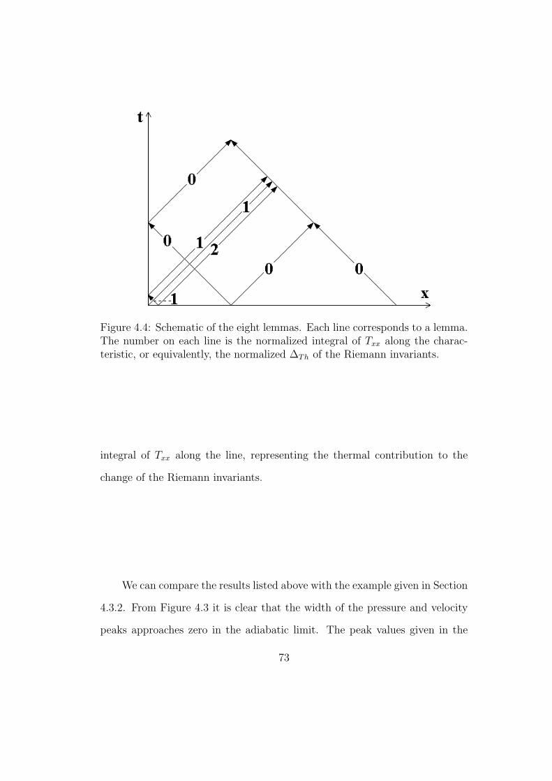
Figure 4.4: Schematic of the eight lemmas. Each line corresponds to a lemma.The number on each line is the normalized integral of Txx along the charac-teristic, or equivalently, the normalized ∆Th of the Riemann invariants.
integral of Txx along the line, representing the thermal contribution to the
change of the Riemann invariants.
We can compare the results listed above with the example given in Section
4.3.2. From Figure 4.3 it is clear that the width of the pressure and velocity
peaks approaches zero in the adiabatic limit. The peak values given in the
73
previous formulas are
limν→0
limx−crt→0+
∆Thpr =1
6, lim
ν→0lim
x−crt→0+∆Thur =
1
6;
limν→0
limx−crt→0−
∆Thpr = − 1
12, lim
ν→0lim
x−crt→0−∆Thur = − 1
12;
limν→0
limx+clt→0−
∆Thpl = −1
3, lim
ν→0lim
x+clt→0−∆Thul =
1
3;
limν→0
limx+clt→0+
∆Thpl = − 1
12, lim
ν→0lim
x+clt→0+∆Thul =
1
12.
They all agree with the solutions shown in Figure 4.3. The peak on the mid
side of the left shock front is invisible because it has the same sign as the peak
value on the other side of the front.
We can further investigate the profile of the pressure peak in the adi-
abatic limit. We prove below that the width of the pressure peaks in the
adiabatic limit is ν/c rather than√
νt, which is the width of the thermal layer
at interface.
Lemma 4.3.9 If x > ct and ε = x− ct = k νc, then
limν→0
∫ t
0
x + c(τ − t)
τ√
4πντexp(−(x + c(τ − t))2
4ντ)dτ = 2e−k.
Proof: As in Lemma 4.3.6,
limν→0
∫ t
0
x + c(τ − t)
τ√
4πντexp(−(x + c(τ − t))2
4ντ)dτ
= limν→0
∫ t
0
ε
τ√
4πντexp(−(ε + cτ)2
4ντ)dτ + lim
ν→0
∫ t
0
c√4πντ
exp(−(ε + cτ)2
4ντ)dτ
74
The first term
limν→0
∫ t
0
ε
τ√
4πντexp(−(ε + cτ)2
4ντ)dτ
=2√π
limν→0
e−cε2ν
∫ ∞
ε√4νt
e−y2
exp(−(cε
4νy)2)dy
=2√π
limν→0
e−k2
∫ ∞
kc
√ν4t
e−y2
exp(−(k
4y)2)dy
= e−k2
2√π
∫ ∞
0
e−y2
exp(−(k
4y)2)dy.
We can do the integration as following. Let
I(k) =2√π
∫ ∞
0
e−y2
exp(−(k
4y)2)dy.
We know I(0) = erf(∞) = 1, and
I ′(k) =2√π
∫ ∞
0
e−y2
exp(−(k
4y)2)(− k
8y2)dy
= − 2√π
∫ ∞
0
exp(−(k
4z)2)e−z2 dz
2
= −1
2I(k).
So I(k) = exp(−k2) and the first term is e−k.
75
Similarly, the second term
limν→0
∫ t
0
c√4πντ
exp(−(ε + cτ)2
4ντ)dτ
=2√π
limν→0
e−cε2ν
∫ c2
√tν
0
e−y2
exp(−(cε
4νy)2)dy
= e−k2 I(k)
= e−k.
From Lemma 4.3.1 and 4.3.9 we know for x > crt and (x−crt)cr
νrfixed,
limν→0
∆Thpr(t, x) = Γr(ρcp)r(Tm − Tr0) exp(− cr
νr
(x− crt)),
limν→0
∆Thpr(t, x) =1
mr
Γr(ρcp)r(Tm − Tr0) exp(− cr
νr
(x− crt)).
Similar formula can be written for the left waves. The profiles of pressure
and velocity peaks on the mid state side are more complicated integral forms
rather than exponential function, yet the width of the peaks are also of the
order of ν/c.
To summarize it, in the limit of vanishing thermal conductivity, the pres-
sure and velocity waves are the same as in the classical Riemann solution
except near the wave fronts, where the peak values can be calculated directly
from the initial conditions and thermodynamic parameters for the linearized
system, and the widths of the peaks are of order ν/c.
76
4.3.4 Asymptotic Solution in the Isothermal Limit
Next let us investigate the asymptotic solution as t → 0 while all para-
meters are fixed. It is equivalent to the limit of ν → ∞ after certain scaling,
so it can also be called the isothermal limit. In our linearized system, we are
looking for limt→0 T (t, 0), limt→0 p(t, 0) and limt→0 u(t, 0) with piecewise con-
stant initial conditions. Although it seems like the classical Riemann problem,
the intrinsic non-localness of parabolic equation (propagation speed is infinity)
changes the solution quite a bit. Without heat conduction the mid state of
the Riemann problem gives continuous pressure and velocity but discontinu-
ous temperature at the contact, while with heat conduction the temperature is
forced to be continuous at the contact, whose value is given in Eq. (4.30). The
subsequent temperature wave shifts the contact pressure and velocity from the
classical mid state. The difference is the ∆Th of the corresponding quantity,
whose values are actually already given in the previous section.
limt→0
T (t, 0) = Tm =Tl0
√(ρcpκ)l + Tr0
√(ρcpκ)r√
(ρcpκ)l +√
(ρcpκ)r
,
limt→0
∆Thp(t, 0) =mrΓl(ρcp)l(Tm − Tl0) + mlΓr(ρcp)r(Tm − Tr0)
mr + ml
= (Tr0 − Tl0)mrΓl(ρcp)l
√(ρcpκ)r −mlΓr(ρcp)r
√(ρcpκ)l
(mr + ml)(√
(ρcpκ)l +√
(ρcpκ)r),
limt→0
∆Thu(t, 0) =Γl(ρcp)l(Tm − Tl0)− Γr(ρcp)r(Tm − Tr0)
mr + ml
= (Tr0 − Tl0)Γl(ρcp)l
√(ρcpκ)r + Γr(ρcp)r
√(ρcpκ)l
(mr + ml)(√
(ρcpκ)l +√
(ρcpκ)r). (4.33)
We can compare these results with the example given in Section 4.3.2.
77
The formulas above predicts
limt→0
T (t, 0) =2
3,
limt→0
∆Thp(t, 0) = − 1
12,
limt→0
∆Thu(t, 0) = −1
4,
which agree with the t = 0 curves in Figure 4.2.
We can also investigate the profile of the pressure wave in the limit of
t → 0. At time t the width of the pressure and velocity waves at the origin is
of order√
νt, and the wave front has moved by ct ¿ √νt, so the wave profile
is dominated by the thermal conduction. We can derive the exact profile as
following.
Lemma 4.3.10 For x = k√
νt,
limt→0
∫ t
0
x + c(τ − t)
τ√
4πντexp(−(x + c(τ − t))2
4ντ)dτ = 1− erf(
k
2).
Proof: Denote x− ct by ε as usual,
limt→0
∫ t
0
x + c(τ − t)
τ√
4πντexp(−(x + c(τ − t))2
4ντ)dτ
= limt→0
∫ t
0
ε
τ√
4πντexp(−(ε + cτ)2
4ντ)dτ + lim
t→0
∫ t
0
c√4πντ
exp(−(ε + cτ)2
4ντ)dτ
78
The first term
limt→0
∫ t
0
ε
τ√
4πντexp(−(ε + cτ)2
4ντ)dτ
=2√π
limt→0
e−cε2ν
∫ ∞
ε√4νt
e−y2
exp(−(cε
4νy)2)dy
=2√π
∫ ∞
k2
e−y2
dy
= 1− erf(k
2).
Similarly, the second term is zero.
Since the lemma is independent of c, for x = k√
νt we also have
limt→0
∫ t
0
x− c(τ − t)
τ√
4πντexp(−(x− c(τ − t))2
4ντ)dτ = 1− erf(
k
2).
Therefore, as x/√
νrt is fixed,
limt→0
∆Thpr(t, x) = Γr(ρcp)r(Tm − Tr0)(1− erf(x
2√
νrt)),
limt→0
∆Thur(t, x) = 0.
The pressure and velocity between −clt and crt are given in Eq. (4.33).
Figure 4.5 shows the plots of pressure and velocity as t → 0. The initial
conditions and parameters are given in Eqs. (4.31) and (4.32). In the figures ν
is inversely proportional to t such that the length scale of diffusion√
νt is fixed
for direct comparison. As t → 0, the pressure profile approaches the formulas
given above (the curve of the formulas, if plotted, would be indistinguishable
79
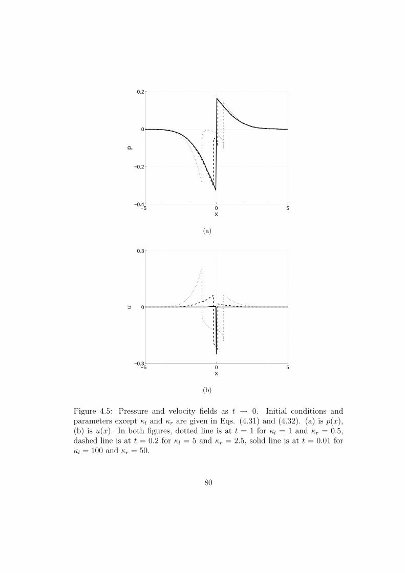
−5 0 5−0.4
−0.2
0
0.2
x
p
(a)
−5 0 5−0.3
0
0.3
x
u
(b)
Figure 4.5: Pressure and velocity fields as t → 0. Initial conditions andparameters except κl and κr are given in Eqs. (4.31) and (4.32). (a) is p(x),(b) is u(x). In both figures, dotted line is at t = 1 for κl = 1 and κr = 0.5,dashed line is at t = 0.2 for κl = 5 and κr = 2.5, solid line is at t = 0.01 forκl = 100 and κr = 50.
80
from the solid line). And the instantaneous mid state does agrees with Eq.
(4.33).
Finally, it should be pointed out that the contact is moving together with
the flow. In the linearized model, i.e. up to the first order of the perturbation,
the contact is moving with the velocity u(t, 0) obtained above.
4.4 Analytical Solution for Phase Transitions: Temper-
ature Field Decoupled
During phase transitions, the mass flux across the phase boundary de-
pends on the interface temperature and the vapor pressure, so the tempera-
ture is coupled to the pressure at the interface even though it is assumed to be
decoupled in both phases. Hence the linearized Euler equations are not readily
solvable as for the contact, yet with certain approximations we can still obtain
the analytical solutions for the special cases.
First, since the heat capacity of the liquid is much larger than that of
the vapor, the interfacial temperature is almost the same as the liquid tem-
perature, which is widely assumed in literatures on bubbly flows [12]. With
this assumption the equation on the temperature field in the vapor is sep-
arated from the pressure field and can be solved analytically. It is a good
approximation for short time, but not for longer time. As we will see later for
nonlinear equations, the interface temperature gradually approaches the sat-
uration temperature of the vapor pressure. Secondly, since the vapor velocity
relative to the phase boundary is much larger than the liquid velocity relative
81
to the boundary due to their large density ratio, we can approximately take
the velocity of the phase boundary, denoted by σ, to be 0 if we only solve the
equations for the vapor.
Assume the vapor is on the right side. For clarity the equations for the
vapor in the characteristic form are rewritten below. Since the equations are
on the vapor side only, the subscripts have been dropped. All thermodynamic
parameters are for the vapor.
∂(p + mu)
∂t+ c
∂(p + mu)
∂x= Γκ
∂2T
∂x2,
∂(p−mu)
∂t− c
∂(p−mu)
∂x= Γκ
∂2T
∂x2,
ρcp∂T
∂t= κ
∂2T
∂x2,
with Cauchy data
(p, u, T )(t = 0) = (p0, u0, T0).
The condition at the phase boundary is
T (t, x = 0) = Tl,
and from Eq. (4.10),
Mev = ρubd = αpsat(Tl)− pv√
2πRT,
82
or equivalently,
µmu(t, 0) = µρ√
γRTu(t, 0) = psat(Tl)− p(t, 0), (4.34)
where µ = 1α
√2πγ
is a dimensionless constant.
4.4.1 Analytical Solution
Similarly we can write down the analytical solution.
T (t, x) = Tl + (T0 − Tl)erf(x√4νt
),
(p−mu)(t, x) = p0 −mu0 − Γκ(T0 − Tl)
∫ t
0
x− c(τ − t)
ντ√
4πντe−
(x−c(τ−t))2
4ντ dτ,
(p + mu)(t, x)|x>ct = p0 + mu0 − Γκ(T0 − Tl)
∫ t
0
x + c(τ − t)
ντ√
4πντe−
(x+c(τ−t))2
4ντ dτ.
(p + mu)(t, x)|x<ct = p(t− x
c, 0) + mu(t− x
c, 0)
−Γκ(T0 − Tl)
∫ t
t−xc
x + c(τ − t)
ντ√
4πντe−
(x+c(τ−t))2
4ντ dτ.
And
p(t, 0) =µpct(t) + psat(Tl)
µ + 1
u(t, 0) =psat(Tl)− pct(t)
(µ + 1)m, (4.35)
where
pct(t) = p0 −mu0 − Γκ(T0 − Tl)
∫ t
0
−c(τ − t)
ντ√
4πντe−
(c(τ−t))2
4ντ dτ
83
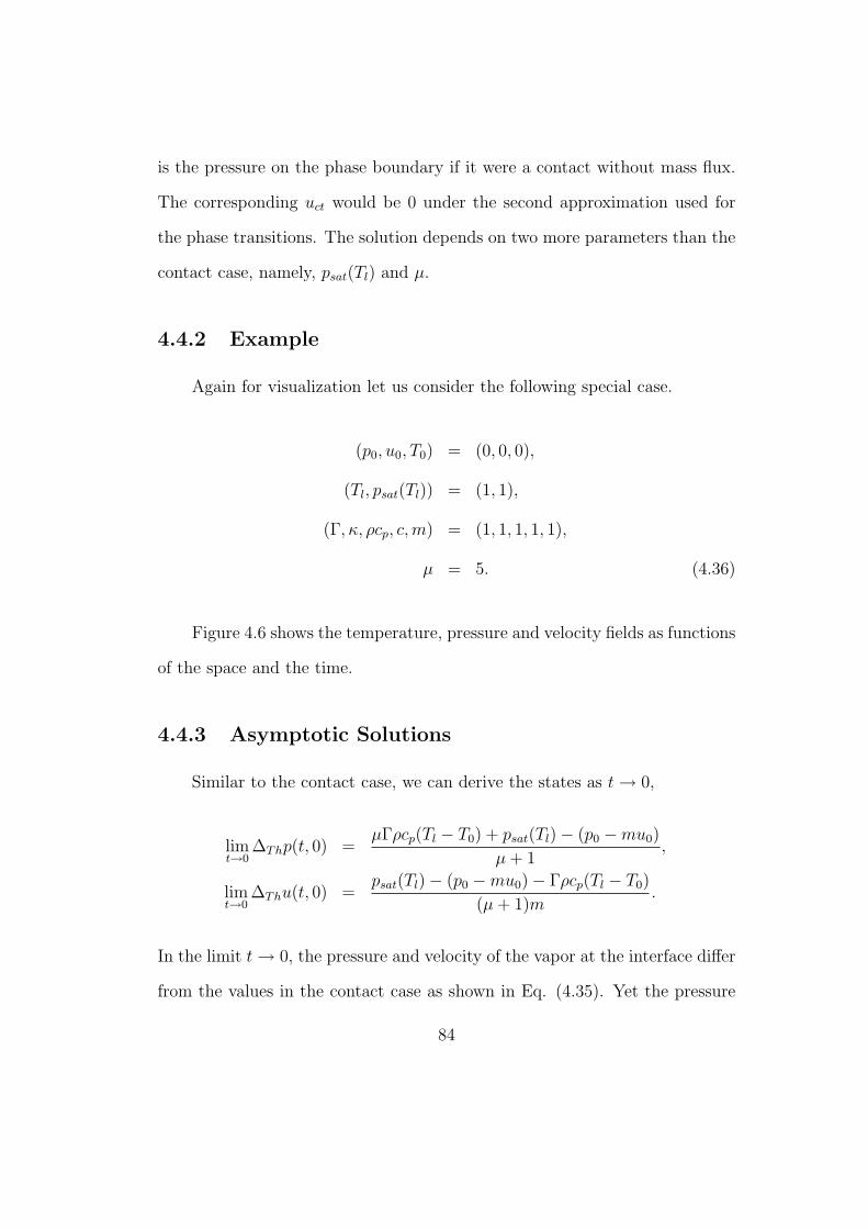
is the pressure on the phase boundary if it were a contact without mass flux.
The corresponding uct would be 0 under the second approximation used for
the phase transitions. The solution depends on two more parameters than the
contact case, namely, psat(Tl) and µ.
4.4.2 Example
Again for visualization let us consider the following special case.
(p0, u0, T0) = (0, 0, 0),
(Tl, psat(Tl)) = (1, 1),
(Γ, κ, ρcp, c, m) = (1, 1, 1, 1, 1),
µ = 5. (4.36)
Figure 4.6 shows the temperature, pressure and velocity fields as functions
of the space and the time.
4.4.3 Asymptotic Solutions
Similar to the contact case, we can derive the states as t → 0,
limt→0
∆Thp(t, 0) =µΓρcp(Tl − T0) + psat(Tl)− (p0 −mu0)
µ + 1,
limt→0
∆Thu(t, 0) =psat(Tl)− (p0 −mu0)− Γρcp(Tl − T0)
(µ + 1)m.
In the limit t → 0, the pressure and velocity of the vapor at the interface differ
from the values in the contact case as shown in Eq. (4.35). Yet the pressure
84
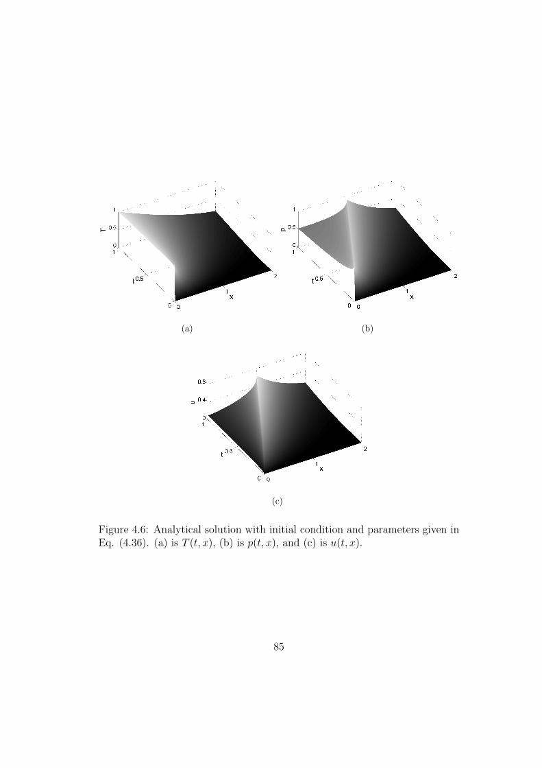
(a) (b)
(c)
Figure 4.6: Analytical solution with initial condition and parameters given inEq. (4.36). (a) is T (t, x), (b) is p(t, x), and (c) is u(t, x).
85
has the same profile of width√
νt as in the contact case. On the other hand,
in the adiabatic limit,
limν→0
limx−ct→0+
∆Thp = Γρcp(Tl − T0),
limν→0
limx−ct→0+
∆Thu =1
mΓρcp(Tl − T0),
limν→0
limx−ct→0−
∆Thp =µΓρcp(Tl − T0) + psat(Tl)− (p0 −mu0)
µ + 1,
limν→0
limx−crt→0−
∆Thu =µΓρcp(Tl − T0) + psat(Tl)− (p0 −mu0)
(µ + 1)m.
For x > ct the ∆Thp and ∆Thu vanish in the adiabatic limit as in the contact
case, but for 0 < x < ct it is not so. In particular, for x = 0,
limν→0
∆Thp(t, 0) =psat(Tl)− (p0 −mu0)
µ + 1,
limν→0
∆Thu(t, 0) =psat(Tl)− (p0 −mu0)
(µ + 1)m.
Distinct from the contact case, the pressure and velocity on the phase bound-
ary do not reduce to the classical Riemann solution in the adiabatic limit. This
result is based on the assumption that the interface temperature is constant.
If the assumption is violated, the interface pressure in the adiabatic limit could
agree with the classical Riemann solution. All the states listed above in the
two limits have been verified for the given example as we did for the contact
case.
Now let us discuss the effect of the parameter µ. Since µ is inversely pro-
portional to the evaporation coefficient, µ → ∞ means no evaporation, thus
reduces to case of contact with thermal conduction, as reflected in Eq. (4.35).
86
On the other hand, if µ → 0, then the vapor pressure is forced to be at equi-
librium with the saturation pressure at the interfacial temperature to induce
a finite evaporation/condensation rate. It is a crude model of evaporation,
which is used literatures such as [24]. In reality, µ is a finite number and its
effect is between these two limit cases.
4.5 Analytical Solutions: Hyperbolic Fields Decoupled
4.5.1 Immiscible Fluids
Next we consider the case that Γ vanishes, again for contact with thermal
conduction first. The linearized equations are
∂(pi + miui)
∂t+ ci
∂(pi + miui)
∂x= 0,
∂(pi −miui)
∂t− ci
∂(pi −miui)
∂x= 0,
(ρcp)i∂Ti
∂t− (βT )i
∂pi
∂t= κi
∂2Ti
∂x2,
where i = l or r. Initial conditions are
(pl, ul, Tl)(t = 0) = (pl0, ul0, Tl0)
(pr, ur, Tr)(t = 0) = (pr0, ur0, Tr0).
Analytical solution
The pressure and velocity fields are exactly the same as the classical Rie-
mann solution. For x > crt, (p, u) = (pr0, ur0). For x < −crt, (p, u) = (pl0, ul0).
87
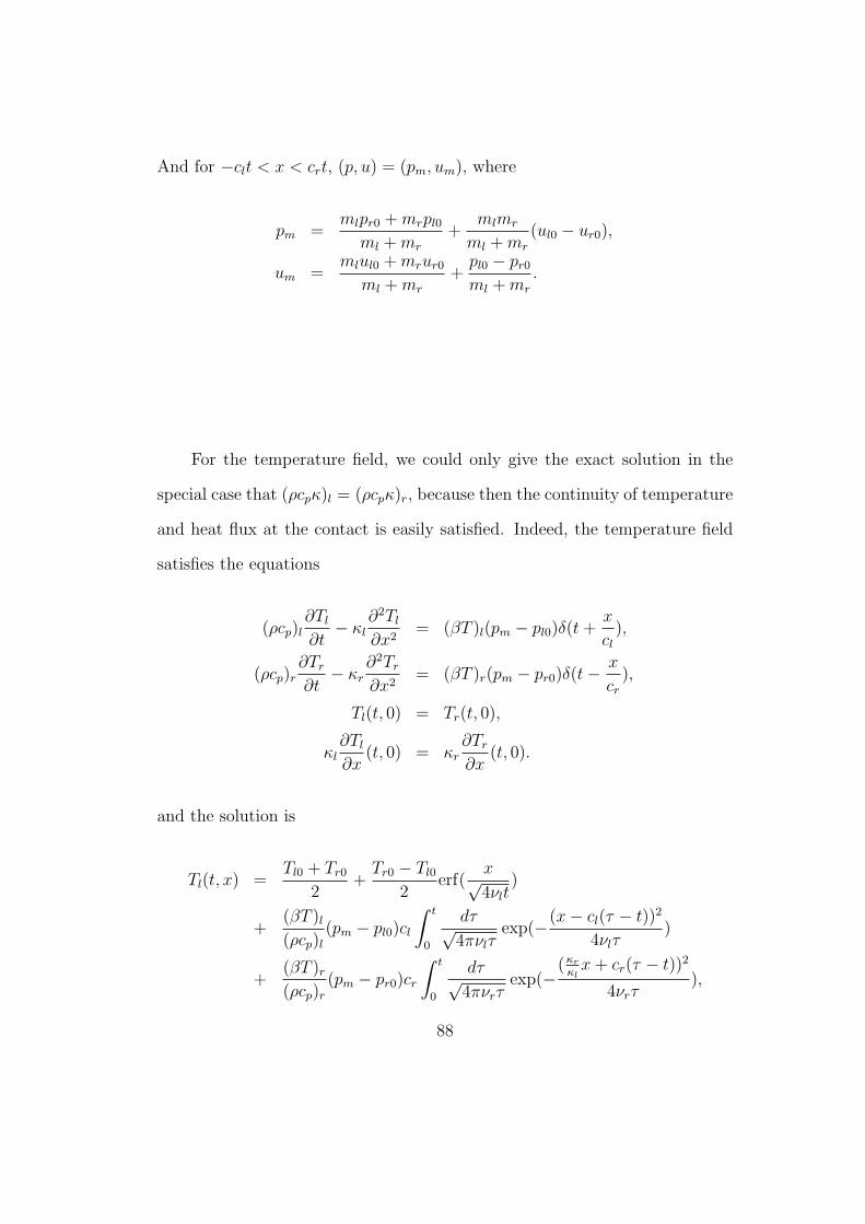
And for −clt < x < crt, (p, u) = (pm, um), where
pm =mlpr0 + mrpl0
ml + mr
+mlmr
ml + mr
(ul0 − ur0),
um =mlul0 + mrur0
ml + mr
+pl0 − pr0
ml + mr
.
For the temperature field, we could only give the exact solution in the
special case that (ρcpκ)l = (ρcpκ)r, because then the continuity of temperature
and heat flux at the contact is easily satisfied. Indeed, the temperature field
satisfies the equations
(ρcp)l∂Tl
∂t− κl
∂2Tl
∂x2= (βT )l(pm − pl0)δ(t +
x
cl
),
(ρcp)r∂Tr
∂t− κr
∂2Tr
∂x2= (βT )r(pm − pr0)δ(t− x
cr
),
Tl(t, 0) = Tr(t, 0),
κl∂Tl
∂x(t, 0) = κr
∂Tr
∂x(t, 0).
and the solution is
Tl(t, x) =Tl0 + Tr0
2+
Tr0 − Tl0
2erf(
x√4νlt
)
+(βT )l
(ρcp)l
(pm − pl0)cl
∫ t
0
dτ√4πνlτ
exp(−(x− cl(τ − t))2
4νlτ)
+(βT )r
(ρcp)r
(pm − pr0)cr
∫ t
0
dτ√4πνrτ
exp(−(κr
κlx + cr(τ − t))2
4νrτ),
88
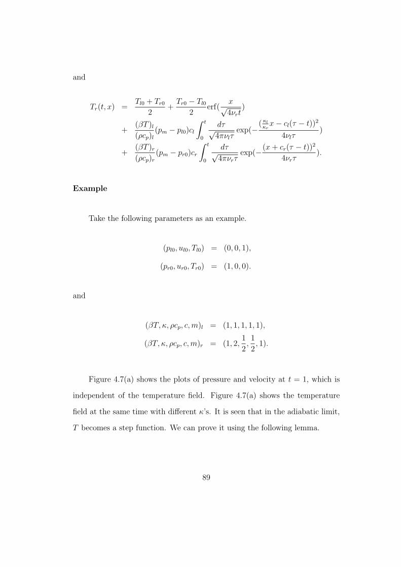
and
Tr(t, x) =Tl0 + Tr0
2+
Tr0 − Tl0
2erf(
x√4νrt
)
+(βT )l
(ρcp)l
(pm − pl0)cl
∫ t
0
dτ√4πνlτ
exp(−( κl
κrx− cl(τ − t))2
4νlτ)
+(βT )r
(ρcp)r
(pm − pr0)cr
∫ t
0
dτ√4πνrτ
exp(−(x + cr(τ − t))2
4νrτ).
Example
Take the following parameters as an example.
(pl0, ul0, Tl0) = (0, 0, 1),
(pr0, ur0, Tr0) = (1, 0, 0).
and
(βT, κ, ρcp, c, m)l = (1, 1, 1, 1, 1),
(βT, κ, ρcp, c, m)r = (1, 2,1
2,1
2, 1).
Figure 4.7(a) shows the plots of pressure and velocity at t = 1, which is
independent of the temperature field. Figure 4.7(a) shows the temperature
field at the same time with different κ’s. It is seen that in the adiabatic limit,
T becomes a step function. We can prove it using the following lemma.
89
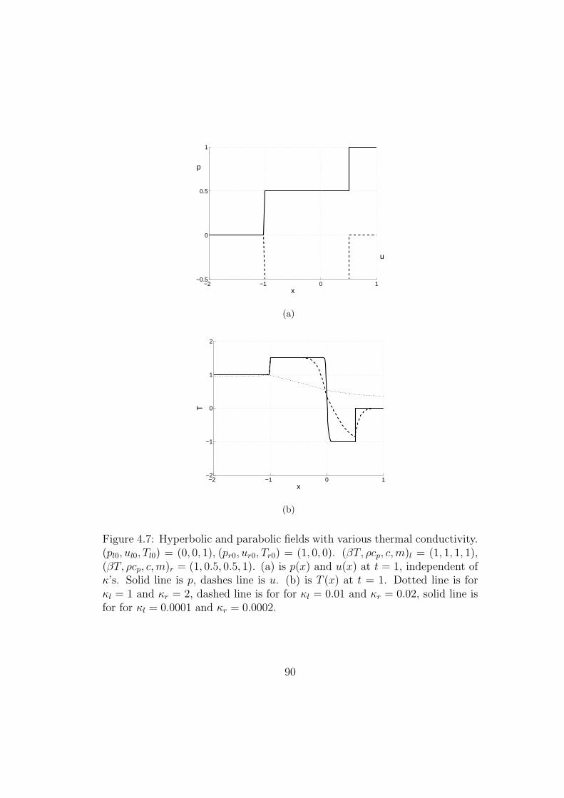
−2 −1 0 1−0.5
0
0.5
1
x
p
u
(a)
−2 −1 0 1−2
−1
0
1
2
x
T
(b)
Figure 4.7: Hyperbolic and parabolic fields with various thermal conductivity.(pl0, ul0, Tl0) = (0, 0, 1), (pr0, ur0, Tr0) = (1, 0, 0). (βT, ρcp, c, m)l = (1, 1, 1, 1),(βT, ρcp, c, m)r = (1, 0.5, 0.5, 1). (a) is p(x) and u(x) at t = 1, independent ofκ’s. Solid line is p, dashes line is u. (b) is T (x) at t = 1. Dotted line is forκl = 1 and κr = 2, dashed line is for for κl = 0.01 and κr = 0.02, solid line isfor for κl = 0.0001 and κr = 0.0002.
90
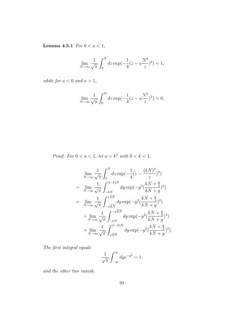
Lemma 4.5.1 For 0 < a < 1,
limN→∞
1√π
∫ N
0
dz exp(−1
4(z − a
N2
z)2) = 1,
while for a < 0 and a > 1,
limN→∞
1√π
∫ N
0
dz exp(−1
4(z − a
N2
z)2) = 0.
Proof: For 0 < a < 1, let a = k2 with 0 < k < 1,
limN→∞
1√π
∫ N
0
dz exp(−1
4(z − (kN)2
z)2)
= limN→∞
1√π
∫ (1−k)N
−kN
dy exp(−y2(kN + y
2
kN + y)2)
= limN→∞
1√π
∫ √kN
−√
kN
dy exp(−y2(kN + y
2
kN + y)2)
+ limN→∞
1√π
∫ −√
kN
−kN
dy exp(−y2(kN + y
2
kN + y)2)
+ limN→∞
1√π
∫ (1−k)N
√kN
dy exp(−y2(kN + y
2
kN + y)2).
The first integral equals
1√π
∫ ∞
−∞dye−y2
= 1,
and the other two vanish.
91
For a < 0,
limN→∞
1√π
∫ N
0
dz exp(−1
4(z − a
N2
z)2)
= limN→∞
1√π
ea2N2
∫ N
0
dz exp(−1
4(z2 + (a
N2
z)2)
≤ limN→∞
1√π
ea2N2
∫ N
0
dze−z2
4
= 0.
For a > 1,
limN→∞
1√π
∫ N
0
dz exp(−1
4(z − a
N2
z)2)
≤ limN→∞
1√π
∫ N
0
dz exp(−1
4((a− 1)N)2)
= limN→∞
N√π
exp(−1
4((a− 1)N)2)
= 0.
Limit solutions
Using the lemma above with N2 = c2tν
and a = 1− |x|ct
, it is straightforward
to show that in the adiabatic limit, the temperature field is
T (t, x < −clt) = Tl0,
T (t,−clt < x < 0) = Tl0 +(βT )l
(ρcp)l
(pm − pl0),
T (t, 0 < x < crt) = Tr0 +(βT )r
(ρcp)r
(pm − pr0),
T (t, crt < x) = Tr0.
92
Compared with the equation on temperature, the formulas above indicate that
the entropy in each phase doesn’t change across the wavefront in the adiabatic
limit, which agree with the classical Riemann solution (for linearized EOS
the entropy jump across the shock front is 0 because the sound speed is a
constant). A refined version of Lemma 4.5.1 would reveal that the transition
layers in terms of a have width of order 1/N and 1/N2 at a = 1 and a = 0,
respectively. For example, it can be proven that for k → 1 while N(1 − k) is
fixed,
limN→∞
1√π
∫ N
0
dz exp(−1
4(z − a
N2
z)2) =
1
2(1 + erf(N(1− k))).
Transformed to the hyperbolic-parabolic system, it means the width of the
left and right propagating temperature jumps are of order ν/c while the jump
width at contact is of order√
νt. This result is the same as the case where βT
is neglected. It is also observed that in the adiabatic limit, the contribution to
the temperature field around the contact from the pressure field has the same
profile as that from the thermal diffusion, namely
T = TM + ∆T erf(x√4νt
), (4.37)
where TM and ∆T are the contact temperature and temperature jump on
either side.
We can also check the isothermal limit, i.e. t → 0. Figure 4.8 shows the
temperature field in the decreasing times with νt fixed. It is easy to see that
93
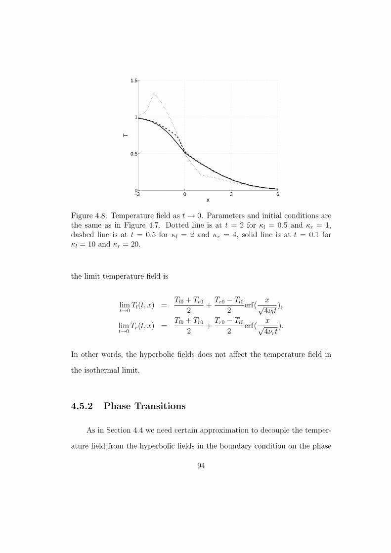
−3 0 3 60
0.5
1
1.5
x
T
Figure 4.8: Temperature field as t → 0. Parameters and initial conditions arethe same as in Figure 4.7. Dotted line is at t = 2 for κl = 0.5 and κr = 1,dashed line is at t = 0.5 for κl = 2 and κr = 4, solid line is at t = 0.1 forκl = 10 and κr = 20.
the limit temperature field is
limt→0
Tl(t, x) =Tl0 + Tr0
2+
Tr0 − Tl0
2erf(
x√4νlt
),
limt→0
Tr(t, x) =Tl0 + Tr0
2+
Tr0 − Tl0
2erf(
x√4νrt
).
In other words, the hyperbolic fields does not affect the temperature field in
the isothermal limit.
4.5.2 Phase Transitions
As in Section 4.4 we need certain approximation to decouple the temper-
ature field from the hyperbolic fields in the boundary condition on the phase
94
boundary. The equation is in the vapor side only, and the approximation is
T (t, 0) = Tl and σ = 0. For clarity, we rewrite the equations here.
∂(p + mu)
∂t+ c
∂(p + mu)
∂x= 0,
∂(p−mu)
∂t− c
∂(p−mu)
∂x= 0,
ρcp∂T
∂t− βT
∂p
∂t= κ
∂2T
∂x2,
with Cauchy data and boundary conditions
(p, u, T )(t = 0) = (p0, u0, T0),
T (t, x = 0) = Tl,
µmu(t, 0) = psat(Tl)− p(t, 0),
where µ = 1α
√2πγ
is a dimensionless constant.
Analytical Solution
The hyperbolic fields are piecewise constant,
p(t, x > ct) = p0,
u(t, x > ct) = u0,
p(t, x < ct) = pm =µ(p0 −mu0) + psat(Tl)
µ + 1,
u(t, x < ct) = um =psat(Tl)− (p0 −mu0)
(µ + 1)m,
95
which agree with Eq. (4.35) derived in the β = 0 case. The temperature is
T (t, x) = Tl + (T0 − Tl)erf(x√4νt
)
+βT
ρcp
(pm − p0)c
∫ t
0
dτ√4πντ
exp(−(x + c(τ − t))2
4ντ)
− βT
ρcp
(pm − p0)c
∫ t
0
dτ√4πντ
exp(−(x− c(τ − t))2
4ντ).
Limit solutions
The limit solutions are nothing but special cases of the previous section
on the contact. In the isothermal limit (t → 0),
limt→0
T (t, x) = Tl + (T0 − Tl)erf(x√4νt
).
In the adiabatic limit,
T (t, x < ct) = T0 +βT
ρcp
(pm − p0),
T (t, x > ct) = T0.
As for the contact case, the formulas indicate that the entropy is continuous
across the wavefront. Notice that the parameters µ and psat(Tl) play no role
in the T field in both limits, although they do affect the pressure and velocity.
Once again, the deviation of the pressure and velocity distributions from the
Riemann solution in the adiabatic limit comes from the assumption that Tl is
a constant.
96
4.6 Full Nonlinear Equations
Having discussed the two exactly solvable cases of linearized equations,
we change gear to the nonlinear equations. The followings are the observations
from the linearized equations.
• In the isothermal limit for immiscible fluids, the thermal effect dom-
inates. The hyperbolic layer (ct) is much narrower than the thermal
layer (√
νt). The pressure has accumulated from the thermal wave an
instantaneous change at each side of the hyperbolic layer, and the mid
state is determined by these modified pressures. The velocity field has
not changed. Both the temperature and the pressure fields in the thermal
layer have width√
νt.
• In the adiabatic limit for immiscible fluids, the solution to the problem
with Riemann data converges to the classical Riemann solution in gen-
eral. The temperature field has jump width of order√
νt at the material
interface and jump width of order ν/c at the propagating shock fronts or
rarefactions. Pressure and velocity fields have spikes at the wave fronts
with width of order ν/c.
• The behavior of the vapor in phase transitions in the isothermal limit
is similar to that for the immiscible fluids but the interface pressure
and velocity are different. At the early stage of phase transitions, the
interface temperature is close to the liquid temperature, but later it
changes slowly toward the saturated temperature at the vapor pressure.
97
As we will see, the solution to the problem with Riemann data also
converges to the classical Riemann solution.
4.6.1 Local Riemann Problem
Next we will give the procedure to solve the full nonlinear local Riemann
problem, being full meaning neither βT nor Γ vanishes. For clearness we
rewrite the equations here.
dp
dλ±± ρc
du
dλ±= Γκ
∂2T
∂x2,
ρcpdT
dλ0
− βTdp
dλ0
= κ∂2T
∂x2. (4.38)
For each phase there is different set of initial conditions and EOS. Subscript
will be added when necessary. Continuity of temperature at the interface
requires an interfacial temperature in the limit t → 0, denoted by Tm. The
procedure is to find the Tm first, then use it to determine the mid state.
The derivation in this section is more heuristic than rigorous compared to the
previous sections.
Temperature field
In the limit of t → 0, the system is predominantly parabolic, so all the
first order spatial derivatives can be neglected. The conservation of mass and
98
momentum gives
∂ρ
∂t= 0, (4.39)
∂(ρu)
∂t= 0, (4.40)
which indicates the density and velocity are unchanged. The energy conserva-
tion law gives
ρcp∂T
∂t= (1 + ΓβT )κ
∂2T
∂x2.
Recalling the thermodynamic identity
cp
cv
=KT
KS
=c2
c2T
= 1 + ΓβT,
where cv is the specific heat with constant volume, cT is the ”isothermal sound
speed”, KT and KS are the isothermal and isentropic compressibility. The
temperature equation can be simplified to
ρcv∂T
∂t= κ
∂2T
∂x2. (4.41)
With Eq. (4.39) in mind, the coefficients in Eq. (4.41) are evaluated
along the isovolumes and thus functions of the only variable T . Therefore it is
a nonlinear equation of T . At the interface T is continuous, and the heat flux
satisfies
κr∂Tr
∂x− κl
∂Tl
∂x= 0 (4.42)
99
for contact, and
κr∂Tr
∂x− κl
∂Tl
∂x= MevL (4.43)
for phase boundary. In case Tl0 = Tr0, we would have Tm = Tl0 = Tr0,
otherwise since the temperature gradient is infinite at the interface as t → 0,
the left side of the Eqs. (4.42) and (4.43) are actually ∞−∞, therefore the
limit temperature field with the boundary condition Eq. (4.43) would have
the same Tm as that with boundary condition Eq. (4.42). In other words, for
the purpose of finding Tm in the limit t → 0, we can always use Eq. (4.42)
instead of Eq. (4.43).
If the coefficients in Eq. (4.41) do not vary much, it suffices to solve the
linearized version. The solution is
Tm =Tl0
√(ρcvκ)l + Tr0
√(ρcvκ)r√
(ρcvκ)l +√
(ρcvκ)r
, (4.44)
Tl(t, x) = Tm + (Tm − Tl0)erf(x√4ν∗l t
),
Tr(t, x) = Tm + (Tr0 − Tm)erf(x√4ν∗r t
),
where ν∗ =√
κ/(ρcv).
Pressure and velocity fields
From the temperature field and Eqs. (4.40) and (4.39), the pressure and
velocity fields outside the hyperbolic layer (x < −clt and x > crt) in the limit
100
t → 0 are
pl(t, x) = Pl(Tl(t, x), ρl0),
pr(t, x) = Pr(Tr(t, x), ρl0),
ul(t, x) = ul0,
ur(t, x) = ur0,
where Pl and Pr are thermodynamic functions depending on the EOS on each
side. Now let us find the mid state in the hyperbolic layer−clt < x < crt. Since
hyperbolic system propagates at finite speed, the local initial value pl(0+, 0−),
ul(0+, 0−), pr(0+, 0+) and ur(0+, 0+) solely determine the instantaneous mid
state. Since the thermal layer is much wider than the hyperbolic layer, the
temperature in the hyperbolic layer is Tm. Therefore the last step is to solve
a Riemann problem with the modification from isentropic to isothermal. The
equations are
∂ρi
∂t+
∂ρiui
∂x= 0,
∂ρiui
∂t+
∂ρiu2i + pi
∂x= 0,
Ti = Tm,
where subscript i is l or r. The initial conditions are
(ρ, p, u)l(t = 0) = (ρl0, Pl(Tm, ρl0), ul0),
(ρ, p, u)r(t = 0) = (ρr0, Pr(Tm, ρr0), ur0).
101
Tm is from the solution to Eq. (4.41) with boundary condition Eq. (4.42).
Approximate value of Tm is given above.
The other conditions at the interface are the Rankine-Hugoniot conditions
for contact
∆p = 0,
∆u = 0,
or Rankine-Hugoniot conditions plus the one from kinetic theory for phase
boundary
∆p = −M∆u, (4.45)
∆u = M∆V, (4.46)
Mev =α√
2πRTm
(psat(Tm)− pv). (4.47)
Here ∆ stands for the difference between left and right side.
Now that the equations are purely hyperbolic, we can find its character-
istics and corresponding ”Riemann” invariants. It it not difficult to show that
the 2 by 2 systems has two characteristics, namely, λ± = u ± cT , where cT is
the isothermal sound speed. The corresponding invariants are du ± dpρcT
. The
solution has self-similarity as in the Riemann problem, so we can construct
the mid state analogously. In Figure 4.9, the curve for left shock wave and
rarefaction passes the (p∗l0, ul0) point in the p−u plane, and the curve for right
shock wave and rarefaction passes the (p∗r0, ur0) point. Here p∗l0 and p∗r0 are
102
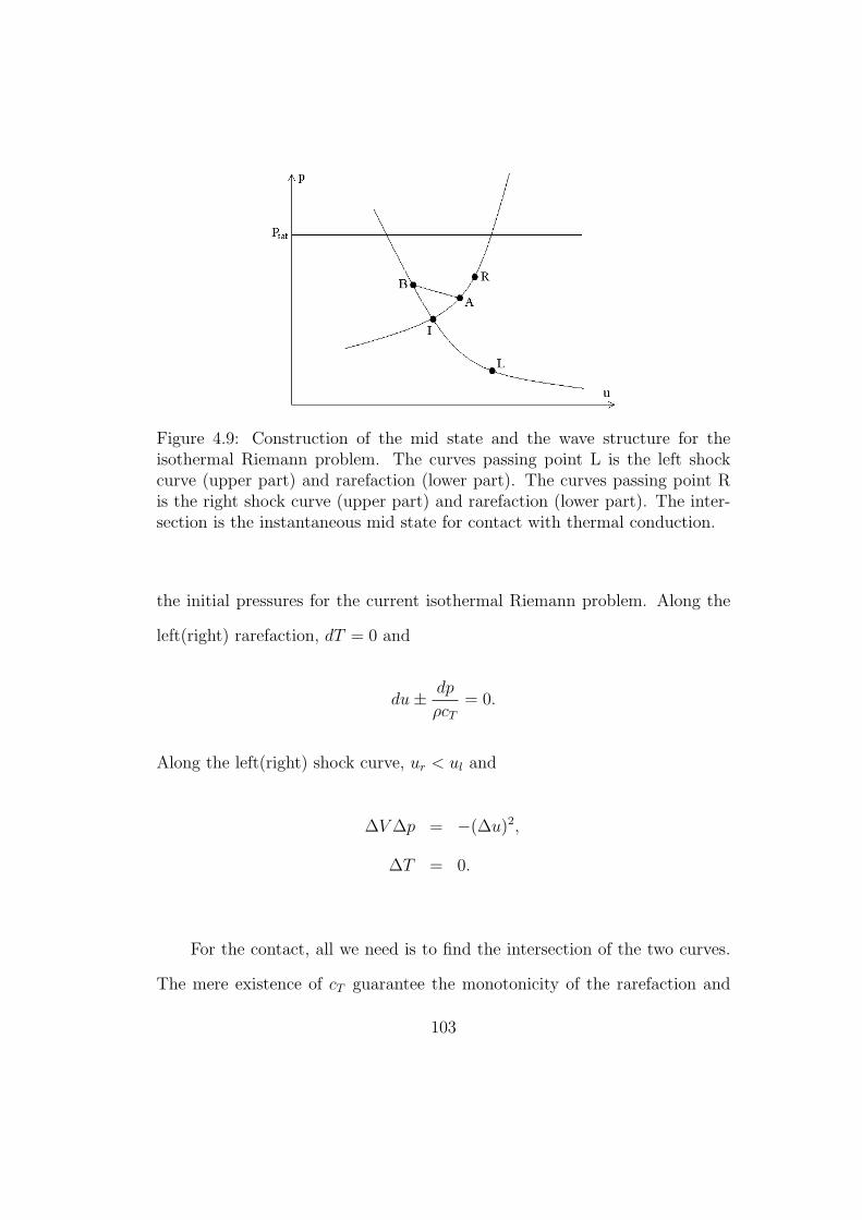
Figure 4.9: Construction of the mid state and the wave structure for theisothermal Riemann problem. The curves passing point L is the left shockcurve (upper part) and rarefaction (lower part). The curves passing point Ris the right shock curve (upper part) and rarefaction (lower part). The inter-section is the instantaneous mid state for contact with thermal conduction.
the initial pressures for the current isothermal Riemann problem. Along the
left(right) rarefaction, dT = 0 and
du± dp
ρcT
= 0.
Along the left(right) shock curve, ur < ul and
∆V ∆p = −(∆u)2,
∆T = 0.
For the contact, all we need is to find the intersection of the two curves.
The mere existence of cT guarantee the monotonicity of the rarefaction and
103
shock curves and thus the uniqueness of the intersection. The mid state is
then determined and the local wave has the same structure as in the Rie-
mann solution, namely, a left shock wave or rarefaction, a right shock wave or
rarefaction, and a contact in between.
Phase transition
For phase transitions, in order to find the left and right mid states we need
to go through the following procedure. For simplicity the vapor is assumed to
be on the right side, the opposite case can be treated similarly.
1. Find the intersection, which is shown as point I in Figure 4.9, of the
curves for left and right waves in p − u plane, just as for the contact.
Denote the mid state by (p∗m, u∗m). If psat(Tm) = p∗m, then from Eq.
(4.47) Mev = 0 and it reduces to the contact without mass flux. If
psat(Tm) 6= p∗m, then go to step 2.
2. We will treat the case psat(Tm) > p∗m, the opposite case can be handled
similarly. For simplicity we will write ps instead of psat(Tm) in this para-
graph. If pv = p∗m, then the vapor is unsaturated, and Eq. (4.47) also
indicates that Mev > 0, so the vapor pressure will increases from the
evaporation. Therefore the actual pv should be between p∗m and ps. We
are going to show that there is a unique pv and associated mid state
satisfying Eqs. (4.45)–(4.47).
For each pv between p∗m and ps we can determine the M = Mev by Eq.
(4.47). The pv also determines uv since (pv, uv), which is point A in
104
Figure 4.9, in one the curve for right wave. Using Eq. (4.45) we can
draw a line with slope −M passing point A. The line would intersect the
curve for left wave so long as M is smaller than the absolute slope of the
curve. Since the latter is approximately ρlcl, it requires
α√2πRTm
(psat(Tm)− pv) < ρlcl,
or equivalently,
α
√γ
2π(psat(Tm)− pv) < ρlclcv,
where γ is the polytropic index of the vapor and cv is vapor sound speed
at temperature Tm. In practice ps is of the same order as pv, and the
inequality above is always satisfied. For example, for water not too far
from saturation in temperature from 20oC to 100oC, the left side of the
inequality is no more than 1 atmosphere, while the right side is more
than 5000 atmosphere. The intersection of the line with the curve is
denoted by point B in Figure 4.9. Now that we know the temporary mid
state on both sides, we can check the last jump condition Eq. (4.46).
Let
f(pv) = ∆u−M∆V.
All quantities on the right side are continuous functions of pv. We need
to find the zero of f for p∗m ≤ pv ≤ ps. Next we will prove the existence
of such a zero point. First, at pv = p∗m, M > 0 by Eq. (4.47) and point
105
A coincides with point B so ∆u = 0, therefore
f(p∗m) = −M(Vv − Vl) < 0,
where we have set the ∆ to be right side minus left side. Second, at
pv = ps, M = 0 by Eq. (4.47) and point B is to the left of point A, so
f(ps) = ∆u = uA − uB > 0.
From fundamental calculus we know f must have a zero between p∗m and
ps. It is easy to verify that f is a monotonely increasing function of pv,
therefore the zero of f is unique. Similar conclusion can be drawn for the
case that ps < p∗m. In that case, Mev < 0 and ps < pv < p∗m. Numerically
the value of pv can be found by iteration. Upon linearization, the Mev
so obtained agrees with the results in Section 4.4.
4.6.2 Travelling Wave Solutions
We sought the solution in the adiabatic limit using the method of trav-
elling wave solutions. The travelling wave solution is a useful tool in the
investigation of nonlinear properties of hyperbolic systems with terms involv-
ing higher order spatial derivatives such as viscosity and thermal conduction
[14, 33]. In this section we studied the travelling wave solutions to the Euler
equations with heat conduction and phase transitions. The equations are Eqs.
(4.1)–(4.3) and the interface conditions are Eqs. (4.4)–(4.10). We first found
106
the travelling wave solutions with the discontinuity at the phase boundary,
then the solutions with the discontinuity in a single phase. Discontinuities
still exist as a contrast to usual travelling wave solutions because here only
the temperature is continuous everywhere while the pressure and velocity are
still allowed to be discontinuous.
Travelling waves across the phase boundary
In the reference frame of the phase boundary, the travelling wave solution
is a steady state. So we only need to find all the steady states. From Eqs.
(4.1)–(4.3), it is easy to write down the solution,
ρu = M,
ρu2 + p = Mu + p = B,
(ρE + p)u− κTx = M(H +u2
2)− κTx = C,
where M , B and C are three constants. The Rankine-Hugoniot conditions
dictates that M , B and C are equal for both left and right states. Since the
interface is at rest, M coincides with the usual notation for mass flux. Using
the remaining two boundary conditions, namely, the continuity of temperature
and Eq. (4.10), the solution is uniquely determined by the pressure, tempera-
ture and temperature gradient of the vapor at the interface. The procedure is
as following. First the M is determined by Eq. (4.10), then the liquid state on
the interface is determined by the continuity of T and the Rankine-Hugoniot
107
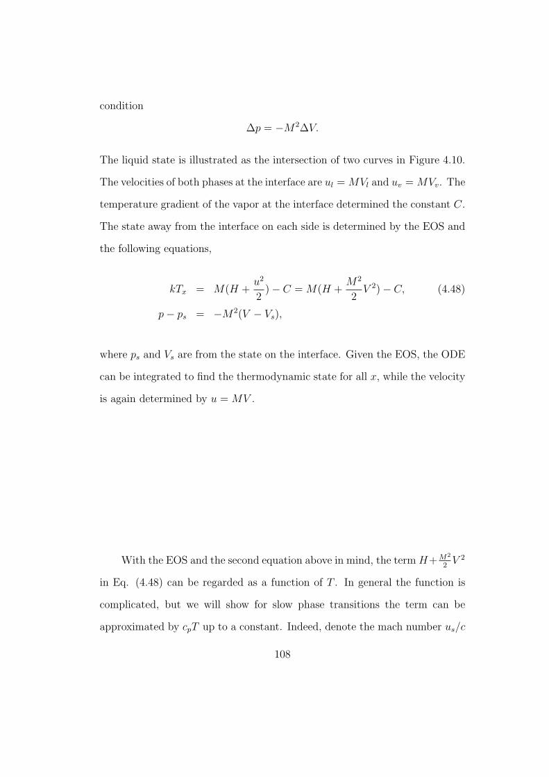
condition
∆p = −M2∆V.
The liquid state is illustrated as the intersection of two curves in Figure 4.10.
The velocities of both phases at the interface are ul = MVl and uv = MVv. The
temperature gradient of the vapor at the interface determined the constant C.
The state away from the interface on each side is determined by the EOS and
the following equations,
kTx = M(H +u2
2)− C = M(H +
M2
2V 2)− C, (4.48)
p− ps = −M2(V − Vs),
where ps and Vs are from the state on the interface. Given the EOS, the ODE
can be integrated to find the thermodynamic state for all x, while the velocity
is again determined by u = MV .
With the EOS and the second equation above in mind, the term H+ M2
2V 2
in Eq. (4.48) can be regarded as a function of T . In general the function is
complicated, but we will show for slow phase transitions the term can be
approximated by cpT up to a constant. Indeed, denote the mach number us/c
108
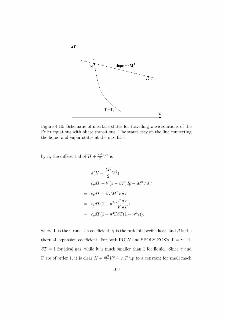
Figure 4.10: Schematic of interface states for travelling wave solutions of theEuler equations with phase transitions. The states stay on the line connectingthe liquid and vapor states at the interface.
by n, the differential of H + M2
2V 2 is
d(H +M2
2V 2)
= cpdT + V (1− βT )dp + M2V dV
= cpdT + βTM2V dV
= cpdT (1 + n2ΓT
V
dV
dT)
= cpdT (1 + n2ΓβT (1− n2γ)),
where Γ is the Gruneisen coefficient, γ is the ratio of specific heat, and β is the
thermal expansion coefficient. For both POLY and SPOLY EOS’s, Γ = γ− 1.
βT = 1 for ideal gas, while it is much smaller than 1 for liquid. Since γ and
Γ are of order 1, it is clear H + M2
2V 2 .
= cpT up to a constant for small mach
109
number.
With the approximation for slow phase transitions, Eq. (4.48) involves
temperature only, so it can be integrated to give
T (x) = Ts +(κTx)s
cpM(exp(
Mcpx
κ)− 1).
The equation above is unbounded for x → ∞ if M > 0 or for x → −∞if M < 0, unless (κTx)s = 0. Therefore, if we require the temperature to
be bounded in the entire space, the ”product” of phase transitions (vapor in
evaporation, liquid in condensation) must be constant state. On the other
hand, if the problem is on a finite domain with certain boundary conditions
to guarantee a steady state solution, both phases can be nonuniform.
To understand the solution, let us take the example of evaporation (M >
0) with constant vapor state. The latent heat for the phase transition is totally
provided by the liquid, i.e.
−(κTx)s = ML.
So the liquid temperature field is
T (x) = Ts +L
cp
(1− exp(Mcpx
κ)). (4.49)
The temperature of the liquid at −∞ is TL = Ts + Lcp
. The interpretation is
clear – the heat released by the liquid whose temperature dropped from TL
to Ts is cp(TL − Ts) = L, which is exact the latent heat needed for the phase
110
transition. Nevertheless, this solution is not physical. The reason is that dur-
ing evaporation, the liquid state on the interface is metastable, and the liquid
state in the above solution has higher temperature but lower pressure than
interface state, which deviates further from the phase coexistence curve and is
metastable or unstable more strongly, so the solution cannot exist physically.
In other word, the physical travelling wave solution can only exist on finite
domain and the ”product” phase cannot be uniform. On the contrary, it is
the ”product” phase that provides the latent heat in evaporation and absorbs
the heat emitted in condensation.
Travelling waves in a single phase
In the reference frame of the pressure jump or equivalently the shock front,
the travelling wave solution is a steady state. The equations are still
ρu = M,
ρu2 + p = Mu + p = B,
(ρE + p)u− κTx = M(H +u2
2)− κTx = C. (4.50)
But now the EOS on both sides of the shock front are the same, and the mach
numbers are bigger than 1 on one side and smaller than 1 on the other. Since
the mach numbers behind the shock is less than 1, the differential of the term
H + M2
2V 2 has the same sign as cpdT . Because the temperature is required
to be bounded in the entire space for a shock wave to exist in the adiabatic
limit, similar to the travelling wave solutions across the phase boundary, we
111
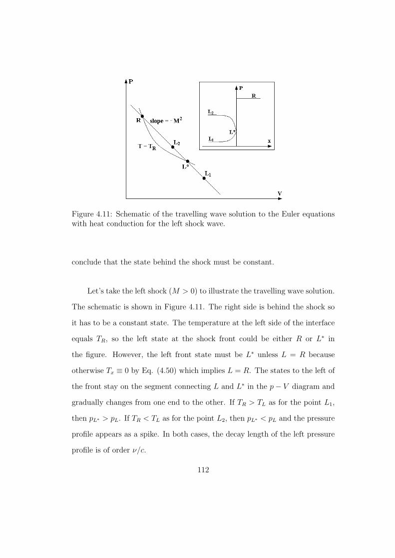
Figure 4.11: Schematic of the travelling wave solution to the Euler equationswith heat conduction for the left shock wave.
conclude that the state behind the shock must be constant.
Let’s take the left shock (M > 0) to illustrate the travelling wave solution.
The schematic is shown in Figure 4.11. The right side is behind the shock so
it has to be a constant state. The temperature at the left side of the interface
equals TR, so the left state at the shock front could be either R or L∗ in
the figure. However, the left front state must be L∗ unless L = R because
otherwise Tx ≡ 0 by Eq. (4.50) which implies L = R. The states to the left of
the front stay on the segment connecting L and L∗ in the p− V diagram and
gradually changes from one end to the other. If TR > TL as for the point L1,
then pL∗ > pL. If TR < TL as for the point L2, then pL∗ < pL and the pressure
profile appears as a spike. In both cases, the decay length of the left pressure
profile is of order ν/c.
112
4.6.3 Adiabatic Limit
In the adiabatic limit, the hyperbolic layer is much wider than the thermal
layers and the solution to the problem with Riemann data essentially has the
same structure as the classical Riemann solution. First we consider the left
and right propagating waves, which are either rarefactions or shock waves. For
rarefactions, the perturbation from the thermal effect approaches zero in the
adiabatic limit because the width of the rarefactions is proportional to t and
much wider than the thermal layers. However for shock waves the perturbation
from the thermal effect does not approach zero everywhere. In fact, from the
travelling wave solutions in a single phase, we see that the pressure wave
deviate from the classical Riemann solution in a region of width about ν/c
and the amount of deviation is nonzero in the adiabatic limit. Next we turn
to the central wave which depends on the interfacial property.
Contact
First we consider the simpler case without phase transition. In the purely
hyperbolic system, the temperature is discontinuous at the contact and the
solution around the contact can be considered as the simplest travelling wave
that has no mass flux. With thermal conduction, however, the temperature
profile at contact is smoothed out to the width of order√
νt, so that the
solution is not a travelling wave solution. The interfacial temperature is de-
termined by temperature on its two sides and the continuity condition of heat
flux. The following is the detail.
The left and right mid states have the same pressure and velocity but
113
different temperature, denoted by TML and TMR. Since the pressure around
the contact is not changing as t →∞, the equations for the temperature are
(ρcp)l(∂Tl
∂t+ ul
∂Tl
∂x) = κl
∂2Tl
∂x2,
(ρcp)r(∂Tr
∂t+ ur
∂Tr
∂x) = κr
∂2Tr
∂x2.
And at contact
Tl = Tr,
κl∂Tl
∂x= κr
∂Tr
∂x.
Also, the temperature at the far left end and the far right end are TML and
TMR respectively. Since the contact is moving together with the fluid, it is
straightforward to show that the temperature at the contact Tct as t →∞ is
Tct =TML
√(ρcpκ)l + TMR
√(ρcpκ)r√
(ρcpκ)l +√
(ρcpκ)r
.
Phase transition
The interfacial temperature is more important for phase transitions be-
cause the transition rate is related to the saturation pressure at the interfacial
temperature. First we exclude the possibility in most cases that the solution
converges to a steady state solution across the phase boundary with nonzero
transition rate. Too see that we assume on the contrary that the solution
does converge to a steady state solution with nonzero mass flux, then as we
114
have pointed out, the ”product” phase must be a constant state, and far from
the phase boundary the ”source” phase has temperature L/cp above/below
the interface temperature for evaporation/condensation, which is unphysical –
e.g. for the phase transition in room temperature between the water and the
water vapor, it requires the source phase to be either the water hotter than
500oC or the vapor colder than −1000oC.
Then we demonstrate that the transition rate decreases to zero as t →∞ and thus the solution is not a travelling wave solution either. The limit
temperature at the phase boundary Tph is determined by
psat(Tph) = pv = pM ,
where pM is the pressure on the contact if there were no phase transition. Again
we assume the vapor is on the right side. Denote the interfacial temperature
by Ts (whose limit as t → ∞ is Tph). The equations for temperature are the
same as for the contact, but the boundary conditions change to
Tl = Tr,
κr∂Tr
∂x− κl
∂Tl
∂x= MevL =
αL√2πRTs
(psat(Ts)− pv). (4.51)
For the moment we assume pv = pM to neglect the interference of the left and
right propagating hyperbolic waves with the thermal wave at phase boundary.
Then using the Tph defined above, the last equation can be rewritten as
κr∂Tr
∂x− κl
∂Tl
∂x=
αL√2πRTs
(psat(Ts)− psat(Tph)).
115
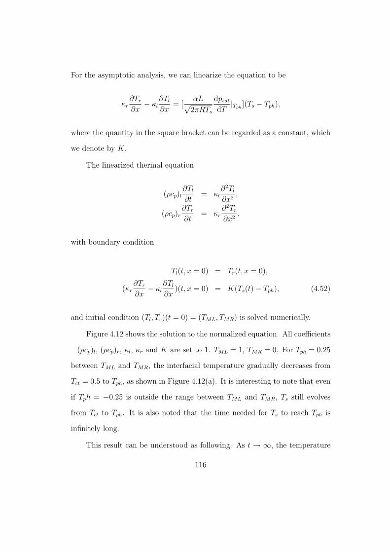
For the asymptotic analysis, we can linearize the equation to be
κr∂Tr
∂x− κl
∂Tl
∂x= [
αL√2πRTs
dpsat
dT|Tph
](Ts − Tph),
where the quantity in the square bracket can be regarded as a constant, which
we denote by K.
The linearized thermal equation
(ρcp)l∂Tl
∂t= κl
∂2Tl
∂x2,
(ρcp)r∂Tr
∂t= κr
∂2Tr
∂x2,
with boundary condition
Tl(t, x = 0) = Tr(t, x = 0),
(κr∂Tr
∂x− κl
∂Tl
∂x)(t, x = 0) = K(Ts(t)− Tph), (4.52)
and initial condition (Tl, Tr)(t = 0) = (TML, TMR) is solved numerically.
Figure 4.12 shows the solution to the normalized equation. All coefficients
– (ρcp)l, (ρcp)r, κl, κr and K are set to 1. TML = 1, TMR = 0. For Tph = 0.25
between TML and TMR, the interfacial temperature gradually decreases from
Tct = 0.5 to Tph, as shown in Figure 4.12(a). It is interesting to note that even
if Tph = −0.25 is outside the range between TML and TMR, Ts still evolves
from Tct to Tph. It is also noted that the time needed for Ts to reach Tph is
infinitely long.
This result can be understood as following. As t → ∞, the temperature
116
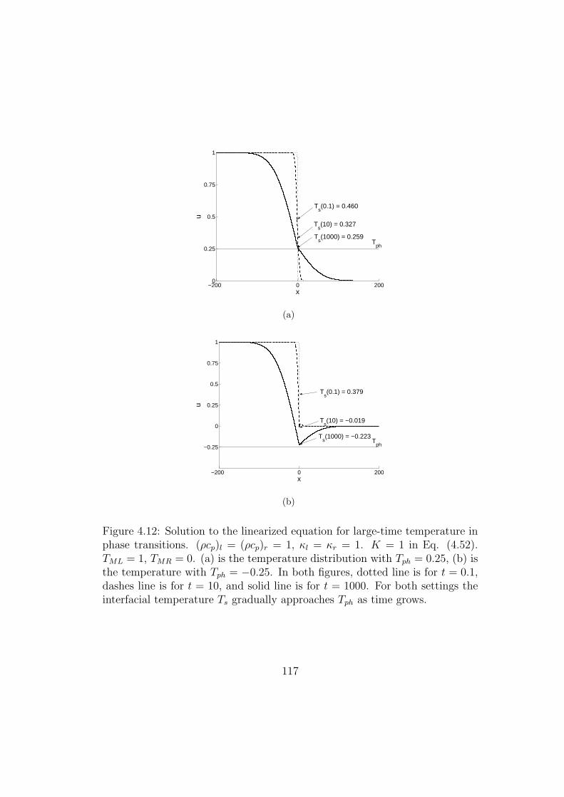
−200 0 2000
0.25
0.5
0.75
1
x
uT
s(0.1) = 0.460
Ts(10) = 0.327
Ts(1000) = 0.259
Tph
(a)
−200 0 200
−0.25
0
0.25
0.5
0.75
1
x
u
Ts(0.1) = 0.379
Ts(10) = −0.019
Ts(1000) = −0.223
Tph
(b)
Figure 4.12: Solution to the linearized equation for large-time temperature inphase transitions. (ρcp)l = (ρcp)r = 1, κl = κr = 1. K = 1 in Eq. (4.52).TML = 1, TMR = 0. (a) is the temperature distribution with Tph = 0.25, (b) isthe temperature with Tph = −0.25. In both figures, dotted line is for t = 0.1,dashes line is for t = 10, and solid line is for t = 1000. For both settings theinterfacial temperature Ts gradually approaches Tph as time grows.
117
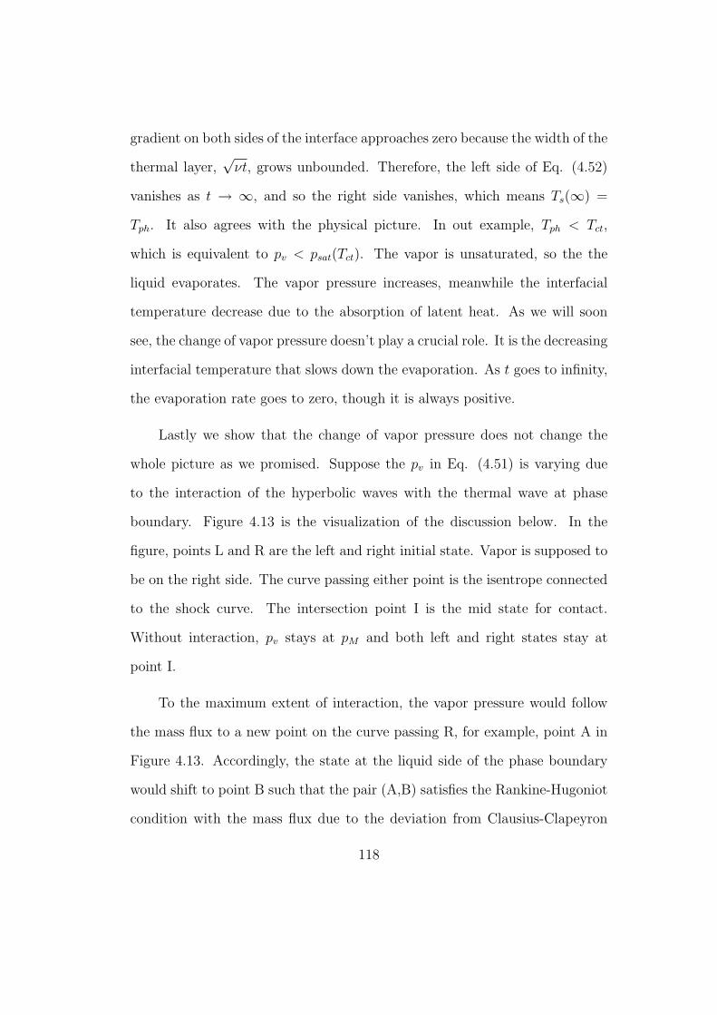
gradient on both sides of the interface approaches zero because the width of the
thermal layer,√
νt, grows unbounded. Therefore, the left side of Eq. (4.52)
vanishes as t → ∞, and so the right side vanishes, which means Ts(∞) =
Tph. It also agrees with the physical picture. In out example, Tph < Tct,
which is equivalent to pv < psat(Tct). The vapor is unsaturated, so the the
liquid evaporates. The vapor pressure increases, meanwhile the interfacial
temperature decrease due to the absorption of latent heat. As we will soon
see, the change of vapor pressure doesn’t play a crucial role. It is the decreasing
interfacial temperature that slows down the evaporation. As t goes to infinity,
the evaporation rate goes to zero, though it is always positive.
Lastly we show that the change of vapor pressure does not change the
whole picture as we promised. Suppose the pv in Eq. (4.51) is varying due
to the interaction of the hyperbolic waves with the thermal wave at phase
boundary. Figure 4.13 is the visualization of the discussion below. In the
figure, points L and R are the left and right initial state. Vapor is supposed to
be on the right side. The curve passing either point is the isentrope connected
to the shock curve. The intersection point I is the mid state for contact.
Without interaction, pv stays at pM and both left and right states stay at
point I.
To the maximum extent of interaction, the vapor pressure would follow
the mass flux to a new point on the curve passing R, for example, point A in
Figure 4.13. Accordingly, the state at the liquid side of the phase boundary
would shift to point B such that the pair (A,B) satisfies the Rankine-Hugoniot
condition with the mass flux due to the deviation from Clausius-Clapeyron
118
Figure 4.13: Schematic of the interaction between hyperbolic waves andthe thermal wave at phase boundary. In the figure psat(Tct) > pM , whichcauses evaporation. The maximum hyperbolic effect would increase pv byδpv ≈ Mevcv.
curve. The difference of point A and B from I is denoted by δp and δu in
Figure 4.13. Since the slope of the curve is approximately ρc,
δpv ≈ ρvcvδuv.
where cv is the vapor sound speed. Taking into account that (ρc)l À (ρc)v,
Rankine-Hugoniot condition ∆u = M∆V gives
δuv ≈ δuv + δul = M(Vv − Vl) ≈ MVv.
Combine the two equations we have
δpv ≈ ρvcvMVv = Mcv.
119
On the other hand, by Eq. (4.34)
µcvM = psat(Ts)− pv = psat(Ts)− pM − δpv,
where µ = 1α
√2πγ
is a dimensionless constant. The last two equation together
gives
cvM =psat(Ts)− pM
µ + 1.
Substituting the equation for M , Eq. (4.51) becomes
κr∂Tr
∂x− κl
∂Tl
∂x= MevL =
L
(µ + 1)cv
(psat(Ts)− pM).
The only difference from the original equation with pv fixed is that µ is replaces
by µ + 1. Therefore, the effect of hyperbolic waves is no more than a reduced
coefficient K. If the hyperbolic interaction is weaker, then the increment from
µ would be less than 1. All in all, a smaller K only slows down the evolution
of Ts to some extent, yet the conclusion that Ts approaches Tph steadily is
sustained. Furthermore, since δpv is proportional to Mev, it also goes to zero
as Mev → 0, which means pv → pM . Therefore the limit state is the same as
without hyperbolic interaction too.
It is worth mentioning that this conclusion shows that the liquid temper-
ature cannot be held to be constant for all time as in Section 4.4. Finally it
should be pointed out that Tph is allowed to be outside the range from TML
to TMR because the waves are propagating in an infinite domain. If the liquid
and vapor, for example, are in an insulated container, then thermal equilibrium
120
will be reached after certain time. In general, the thermal effect eventually
dominates over the hyperbolic effect in isolated systems.
4.6.4 Wave Structure
Now that we have investigated both the short time behavior (isothermal
limit) and the large time behavior(adiabatic limit) of the Euler equations with
thermal conduction, we will discuss the global wave structure at all times. For
t much smaller than the characteristic time ν/c2, thermal effect dominates
and the system is essentially isothermal. For t much larger than that, the
hyperbolic effect dominate and the system is essentially adiabatic. For time
in between, both effects are important.
• For t ¿ ν/c2, ct ¿ √νt and the hyperbolic layer is an isothermal 3-wave
structure embedded in the much wider thermal layer. The left and right
waves propagate at the isothermal sound speeds, and they can be shocks
or rarefactions. The mid state depends on whether the interface is the
contact or the phase boundary. The isothermal waves propagate away
from the interface and determine the size of the spikes at the shock fronts
at later times.
• For t À ν/c2, ct À √νt À ν/c and the hyperbolic layer evolves into
the 3-wave structure of the classical Riemann solution, left and right
waves propagating at the adiabatic sound speeds. If the wave is a shock,
there is a thermal layer of width about ν/c around the shock front, in
which the deviation from the classical Riemann solution can be nonzero
121
in the limit of t → ∞. If the wave is a rarefaction, the thermal layer
can cover the entire rarefaction and the deviation vanishes in the limit of
t →∞. There is no mass flux across the interface at large times for both
the immiscible fluids and the phase transitions, and the thermal layer
around the interface has the width of order√
νt. The only difference
between the two cases is in the interface temperature. For immiscible
fluids it is between the temperature on the two sides of the contact, for
phase transitions it is determined by the saturation condition.
• For intermediate times, ct ≈ √νt ≈ ν/c and the hyperbolic layer still
have the 3-wave structure but it is neither isothermal nor adiabatic.
The left and right waves propagate at varying speeds, which gradually
shift from isothermal to adiabatic. As shown in Figure 4.2, the spikes
at the left and right wave fronts overlap with each other and also with
the thermal layer at the interface. As a result, the solution is far from
being piecewise constant or rarefactions. It is not clear yet whether extra
shocks could exist, good numerical algorithms may help to capture the
detailed wave structure.
122
Chapter 5
Numerical Algorithm for the Simulation of
Phase Transitions
The numerical algorithm for the heat conduction and phase transitions
is based on the front tracking method. A key feature of front tracking is the
avoidance of finite differencing across discontinuities fronts and thus the elim-
ination of interfacial numerical diffusion. Phase boundary is tracked explicitly
by a codimension one grid immersed in a regular spatial grid. The front prop-
agates according to the dynamics around it (i.e. Lagrangian) while the regular
spatial grid is fixed in time (i.e. Eulerian). In each time step, the front is first
propagated with states on its two sides updated, then the interior states are
updated using finite difference scheme.
Section 5.1 is the algorithm for interface propagation and front states up-
date, and Section 5.2 describes the 2nd order finite difference update of the
interior states. The numerical algorithm has been implemented into the Fron-
Tier hydro code. In Section 5.3 we validated the numerical scheme by verifying
the convergence of the simulation results to the analytical solution through
123
mesh refinement, we also illustrated the effectiveness of the thin thermal layer
method. Lastly the numerical method was applied to the one dimensional
condensation problem in Section 5.4.
5.1 Propagation of Phase Boundary
5.1.1 Normal Propagation
The phase boundary is first propagated in the normal direction. The
characteristic form of the equations at the phase boundary has been given in
Eqs. (4.12)–(4.15). Normal propagation solves a non-local Riemann problem.
The original hyperbolic solver has three steps: slope reconstruction, prediction
using a local Riemann solver, and correction by a nonlocal solver.
The first step in hyperbolic solver is kept. The second step has been
modified as following. At the very first time step (dt = 0) or the time step
when the phase boundary is dynamically created, the boundary states are set
as described in Section 4.6.1. If the temperature is continuous across the phase
boundary, nothing need to be done. Otherwise the interface temperature is
calculated by solving the nonlinear Eq. (4.41) or using the approximate value
in Eq. (4.44), while the density and velocity of the states on both sides of the
interface are kept unchanged (the pressure, from EOS, changes accordingly),
thus the left and right states become the point L and R in Figure 4.9. We
could go further to solve the adiabatic Riemann problem exactly as described
in Section 4.6.1, which requires extra iteration for phase transition. However,
the lengthy procedure is skipped. The reason is that if the left and right
124
states were initialized as mid states in Figure 4.9 rather than the L and R
states, the exact value of L and R states wouldn’t be recovered in the finite
difference update in the subsequent time steps due to the singularity of the
temperature field at origin, thus the physical spikes at the shock fronts would
be severely reduced. In fact, the current implementation not only gives more
accurate height of the spikes, but also predicts the correct, though not exact,
mid states from the linearized solver in the subsequent time steps. For all
subsequent time steps, the interfacial pressure, velocity and temperature are
forced to satisfy the required boundary conditions such as Rankine-Hugoniot
condition and phase transition rate equation, so that the local Riemann solver
does not change the states on either side of the interface. Therefore, the normal
velocity of the phase boundary at the beginning of each time step is obtained
from the beginning states directly, and the sound speeds needed for the slopes
of characteristics are also directly from the beginning states on the two sides
of the interface.
In the step of nonlocal solver, a discrete version of the characteristic sys-
tem Eqs. (4.12)–(4.15) is solved. The phase boundary normal velocity ob-
tained at the end of the time step is averaged with the value at the beginning
of the time step and then used for the propagation of phase boundary.
To solve the characteristic system, the states at the feet of the traced back
characteristics are first obtained by interpolation, usually of the conservative
quantities, namely, mass, momentum and total energy density. The charac-
teristic λ± = u± c and λ0 = u, while the material interface move at σ = u for
contact and σ = ∆(ρu)/∆ρ for phase transition. For small time step ∆t, the
125
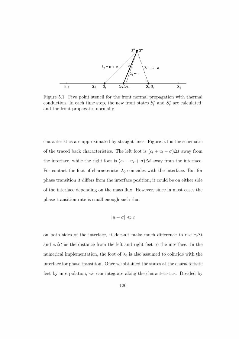
Figure 5.1: Five point stencil for the front normal propagation with thermalconduction. In each time step, the new front states S∗l and S∗r are calculated,and the front propagates normally.
characteristics are approximated by straight lines. Figure 5.1 is the schematic
of the traced back characteristics. The left foot is (cl + ul − σ)∆t away from
the interface, while the right foot is (cr − ur + σ)∆t away from the interface.
For contact the foot of characteristic λ0 coincides with the interface. But for
phase transition it differs from the interface position, it could be on either side
of the interface depending on the mass flux. However, since in most cases the
phase transition rate is small enough such that
|u− σ| ¿ c
on both sides of the interface, it doesn’t make much difference to use cl∆t
and cr∆t as the distance from the left and right feet to the interface. In the
numerical implementation, the foot of λ0 is also assumed to coincide with the
interface for phase transition. Once we obtained the states at the characteristic
feet by interpolation, we can integrate along the characteristics. Divided by
126
ρc and then integrated from t to t + ∆t, Eqs. (4.12) and (4.13) become
∫ t+∆t
t
dp
dλ+
dλ+
ρc+ (u∗l − uf ) + αN0
∫ t+∆t
t
cu
rdλ+
= −∫ t+∆t
t
∂φ
∂ndλ+ −
∫ t+∆t
t
Γ
ρc(∂q
∂n+ αN0
q
r)dλ+,
∫ t+∆t
t
dp
dλ−
dλ−ρc
− (u∗r − ub) + αN0
∫ t+∆t
t
cu
rdλ−
=
∫ t+∆t
t
∂φ
∂ndλ− −
∫ t+∆t
t
Γ
ρc(∂q
∂n+ αN0
q
r)dλ−. (5.1)
Neglecting the distance between the foot of the characteristic λ0 and the in-
terface, we have
u′∗l = u′0−,
u′∗r = u′0+,
where u′ is the tangential velocity. We can also integrate the energy equation,
however since it is a parabolic equation for temperature, the interface state
is preferably determined by boundary condition rather than integration along
λ0. The boundary conditions depends on the interfacial dynamics. The case
of contact is simpler, so we treat it first.
127
Contact with thermal conduction
The boundary conditions are
∆u = 0,
∆p + ps = 0,
∆T = 0,
∆q = 0,
where ps is the pressure jump due to surface tension, which is determined
by the surface tension coefficient and the local curvature on the interface.
The discrete characteristic equation along with the boundary condition can be
solved in several ways. There are three methods implemented for the nonlo-
cal hyperbolic Riemann solver, namely, RIEMANN, MOC+RH and CHEAP
MOC+RH methods [21]. The RIEMANN method exploits the similarity be-
tween Eq. (5.1) and the local Riemann problem. It uses a local Riemann
solver with Sf and Sb as initial left and right states to solve for the mid state.
However it does not readily apply in our situation, because as pointed out in
Section 4.6.4 the nonlocal wave structure is much more complicated than the
local 3-wave structure. The other two methods approximate the the integrals
in Eq. (5.1) by finite differences in time. The only difference between the
them is that MOC+RH uses trapezoidal rule quadrature for the integration
while CHEAP MOC+RH uses backward difference quadrature. In view of
the various first order approximations already made at the interface, there
would be little difference between the two methods. The following procedure
128
is analogous to the CHEAP MOC+RH method.
1. Starting from the usual five point stencil along the normal of the interface
as shown in Figure 5.1. Let the grid size be ∆n. First we determine the
interfacial temperature. The boundary conditions
T ∗l = T ∗
r
κlT ∗
l − T−1
∆n= κr
T1 − T ∗r
∆n
give
Ts := T ∗l = T ∗
r =κlT−1 + κrT1
κl + κr
. (5.2)
2. Next we seek S∗l and S∗r . The difference equations are
p∗l − pf
ρfcf
+ (u∗l − uf ) + αN0cfuf
rf
∆t + (φ′n)f∆t
=Γf
ρfcf
κl(T−2 + T0− − 2T−1
∆n2+ αN0
T0− − T−1
rf∆n)∆t,
p∗r − pb
ρbcb
− (u∗r − ub) + αN0cbub
rb
∆t− (φ′n)b∆t
=Γb
ρbcb
κr(T2 + T0+ − 2T1
∆n2+ αN0
T1 − T0+
rb∆n)∆t.
Combined with u∗l = u∗r and p∗l = p∗r +ps, the pressure and velocity of S∗l
and S∗r is readily solved. Finally the density of the states are determined
from their EOS’s with known pressure and temperature.
129
Phase transition
Next we treat the interfacial propagation for phase transition. The bound-
ary conditions are
∆u = M∆V, (5.3)
∆p + ps = −M2∆V, (5.4)
∆T = 0, (5.5)
∆q = −MevL, (5.6)
Mev =α√
2πRTs
(psat(Ts)− pv). (5.7)
Since the interfacial temperature is coupled to the phase transition rate by
kinetic theory, the temperature cannot be determined directly. Iteration over
the vapor pressure pv and the difference of specific volumes ∆V has been used.
For clearness, we assume the vapor is on the right side.
1. Substituting the vapor pressure at S0+ for the pv in Eq. (5.7) and dis-
cretizing Eq. (5.6), we have two equation for the two variable Ts and
Mev. The equations are
MevL = κrT1 − Ts
∆n− κl
Ts − T−1
∆n,
Mev =α√
2πRTs
(psat(Ts)− pv).
The function psat is a nonlinear function, Newton’s iteration or similar
method is needed to solve the equations exactly. However, since this
step itself is in the iteration of pv and ∆V , we can linearize the Clausius-
130
Clapeyron equation at a reference temperature Tr and solve for Ts and
Mev while preserving the convergence of S∗l and S∗r through the iteration.
For the first iteration step, Tr can be chosen to be the Ts at the beginning
of the time step if T0− = T0+, or their average, for example, (T0−+T0+)/2
if they are different. For subsequent iteration steps, Tr is simply the Ts
obtained in the last iteration. Upon linearization,
Ts =κlT−1 + κrT1 + α√
2πRTrL∆n(pv − psat(Tr) + dpsat
dT(Tr)Tr)
κl + κr + α√2πRTr
L∆ndpsat
dT(Tr)
, (5.8)
and
Mev =α√
2πRTr
(psat(Tr)− pv +dpsat
dT(Tr)(Ts − Tr)),
where dpsat
dT(Tr) is the slope of phase coexistence curve at Tr, which by
Clausius-Clapeyron equation equals
dpsat
dT(Tr) =
L
Tr(Vv(Tr, psat(Tr))− Vl(Tr, psat(Tr))).
2. Having obtained the temperature and mass flux, we can solve the char-
acteristic Eq. (5.1) with the Rankine-Hugoniot conditions Eqs. (5.3)
and (5.4). For the first iteration the ∆V in Eqs. (5.3) and (5.4) is set
to Vr0 − Vl0. Then same as the last step for contact, the density ρ∗l and
ρ∗r are determined from their EOS’s with the pressure and temperature
obtained in the iteration.
3. The last step in the iteration is to compare the newly obtained pv and
∆V with the values used in the iteration. If the differences are within
131
the preset tolerance, then the iteration is over, otherwise update the pv
and ∆V for next iteration and go back to step 1.
In practice it is found that pv and ∆V usually has relative error below 10−6
after 4 iterations. The convergence of pv and ∆V guarantees the convergence
of Ts, thus justifies the linearization of the Clausius-Clapeyron equation used
in step 1.
5.1.2 Thin Thermal Layer Method
The method described above works well for fine grid, but when the grid is
coarse as required by the physical problem or the computational capability, we
have a numerical difficulty. For large ∆n, the interface temperature given in
Eq. (5.8) is approximately Tsat(pv), while in reality it should change gradually
from the Ts given in Eq. (5.2) to Tsat(pv). The wrong interface temperature
would in turn gives wrong temperature and pressure fields, especially in the
liquid. To make it worse, even Eq. (5.2) gives wrong temperature if the
thermal layer is narrower than the grid size, for which the correct interface
temperature is close to
Tm =T−1
√(ρcpκ)l + T1
√(ρcpκ)r√
(ρcpκ)l +√
(ρcpκ)r
.
To illustrate it, let us consider a practical situation. For two dimensional
simulation of bubbly water in a container of size 1cm, suppose the grid size is
dx = 1µm, which is already quite fine. The thermal layer in water is of width√
νt where ν = κ/(ρcp) = 1.5× 10⁻⁶cm2/ms, and the time step restricted by
132
CFL condition is dt = dx/c = 6.7× 10⁻⁷ms. So it requires
dx2
νdt= 104
time steps for the thermal layer to expand to a grid cell. For all these time
steps, it is inappropriate to use simple finite difference for the temperature
gradient at the interface. More details are given in Section 5.3.
To solve the Euler equations with reasonable accuracy in a coarse grid,
we need to represent the thermal layer in certain way. A widely used method
is the spectral method [24, 30, 2], where the temperature field is spanned by
Chebychev polynomials and the evolution is solved by Galerkin method or
collocation method. However, spectral method has several drawback. First,
it has been only used for spherical problems where the temperature field can
be spanned by single variable polynomials, while our goal is to develop direct
numerical simulation scheme in arbitrary geometry. Moreover, the coordinate
of vapor in (0, Rbub] is normalized to (0, 1] for the variable in the polynomials,
while the coordinate of liquid is normalized from [Rbub,∞) to (0, 1], which
cannot be carried out for the multi bubble system we intend to simulate.
Secondly, for the spectral method the temperature field is always separated
from the pressure and velocity waves – in vapor uniform pressure is assumed,
and in liquid the thermal expansion coefficient is set to zero. The evolution
of the pressure field does not depend on temperature either – it is either the
Rayleigh-Plesset equation for incompressible fluid or the Keller equation for
weakly compressible fluid. So the temperature and pressure can be solved
133
on different grids or in different solution spaces. As a contrast, for the fully
compressible fluid we simulate, they have to be solved simultaneously on a
common grid. Spectral method, even if it worked efficiently, would invoke
a difficult problem for mapping the temperature field from the polynomial
expansion form to the fixed grid while preserving the accuracy.
As a result, we hereby present a different method that incorporates the
thermal layer into the finite difference scheme when necessary. The idea is
simple. When the thermal layer is thinner than a grid cell, then the temper-
ature profile should take the form of Eq. (4.37). For clarity, we consider the
phase on the right side of the interface and rewrite the equation with slight
changes in notation,
T = TM + (TR − TM)erf(x√4νt
).
Since the thermal layer is thinner than the grid size dx, the temperature T1
one grid cell away from the interface should be approximately TR. Taking
derivative over x at the origin in the equation above, we have
(∂T
∂x
)
0
= (TR − TM)2√π
1√4νt
≈ T1 − TM√πνt
.
Therefore the temperature gradient at the interface is better approximated by
(T1 − TM)/√
πνt than (T1 − TM)/dx. Considering the approximate nature of
the argument, we used ε√
νt instead of√
πνt in the implementation, where
ε is a number of order 1 to be optimized by numerical experiment. When
ε√
νt is larger than dx, the thermal layer can be regarded as wider than a
134
grid cell, so we can revert to the usual finite difference approximation for
the temperature gradient. As a summary, the temperature gradient at the
interface is approximated by
(∂T
∂x
)
0
≈ T1 − TM
dx∗:=
T1 − TM
min(ε√
νt, dx), (5.9)
where dx∗ is defined to min(ε√
νt, dx). Numerical experiment found ε = 1 is a
good choice in general, so ε is set to 1 by default. Admittedly the uncertainty
of ε makes the method ad-hoc, however as we will see in Section 5.3 it works
quite well in spite of its simplicity. It should be emphasized that the t in the
formulas is the time since the interface in created rather than the global time
if the bubbles are created dynamically as in [22].
When the thin layer modification is applied to the normal front propa-
gation, all interfacial heat flux in the form of κ∆T/∆n should be replaced
by κ∆T/∆n∗ with the ν in the corresponding phase. For example, Eq. (5.2)
should be replaced by
Ts =
κl
∆n∗lT−1 + κr
∆n∗rT1
κl
∆n∗l+ κr
∆n∗r
,
where ∆n∗l = min(ε√
νlt, ∆n) and ∆n∗r = min(ε√
νrt, ∆n). Eq. (5.8) changes
similarly, and so does the heat flux at interface in the characteristic equations.
Another point need to be mentioned is that throughout the analysis on thin
thermal layer, the temperature gradient away from the interface in either phase
has been assumed to be zero. In the general situation that the gradients don’t
vanish, the T1 in Eq. (5.9) for thin thermal layer is not close to TR (the
interface temperature with thermal conduction neglected). Rather, T1 in Eq.
135
(5.9) should be replaced by the appropriate approximation of TR, which is
given by the extrapolation 2T1 − T2. The left side of the interface should
be handled accordingly to give the correct temperature and heat flux on the
interface. For example, the correct form of Eq. (5.2) is
Ts =
κl
∆n∗l(2T−1 − T−2) + κl
∆n(T−2 − T−1) + κr
∆n∗r(2T1 − T2) + κr
∆n(T2 − T1)
κl
∆n∗l+ κr
∆n∗r
.
In the later sections, the numerical technique introduced here will be referred
to as the thin (thermal) layer method.
5.1.3 Tangential Propagation
The normal propagation of the front solves the Euler equations projected
onto the normal direction. After that the Euler equations projected onto the
tangent space are solved on both sides of the front. Along the tangential
direction(s),
∂ρ
∂t+
∂ρu
∂τ+ αN1
ρu
r= 0,
∂ρu
∂t+
∂(ρu2 + p)
∂τ+ αN1
ρu2
r= −ρ
∂φ
∂τ,
∂ρu′
∂t+
∂ρuu′
∂τ+ αN1
ρuu′
r= 0,
∂ρE
∂t+
∂(ρE + p)u
∂τ+ αN1
(ρE + p)u
r= − ∂q
∂τ− αN1
q
r,
where τ is the tangential direction of the interface in two-dimensional problem
or one of the tangential directions in three-dimensional problem. u and u′ are
the tangential velocity along τ and the velocity components perpendicular to
136
τ . q is the tangential heat flux. N1 is the x component of the τ .
The tangential equations are solved using the finite difference scheme
described in the next section. The only difference between tangential state
update and interior state update is that the N1 for interior update is either 0
or 1. After the tangential propagation, the states on the two sides of the front
are changed, so the Rankine-Hugoniot conditions, temperature continuity and
the equations about heat flux and phase transition rate could be violated. An
extra normal propagation with ∆t = 0 after the tangential propagation solves
the problem.
5.2 Finite Difference Update of Interior States
After the front propagation and update of front states, the interior states
on the spatial grid need to be time updated. Since the heat conduction does
not involve cross derivatives in space, we can still use directional splitting as
in the current implementation. The advantage of weaving the parabolic terms
into the hyperbolic step rather than after it is that the accuracy of the scheme
is boosted from 1st order to 2nd order in time.
The shock capturing methods currently implemented in FronTier for one-
dimensional sweeps include Lax-Wendroff method, Lax-Friedrichs method,
Collela piecewise linear method and a second order monotone upwind scheme
for conservation laws (MUSCL) scheme developed by Van Leer and adapted
for FronTier by I-L. Chern. MUSCL scheme is similar to the piecewise par-
abolic method described in [11], and a detailed description can be found in
[10]. The two-pass implementation currently being used in FronTier, namely,
137
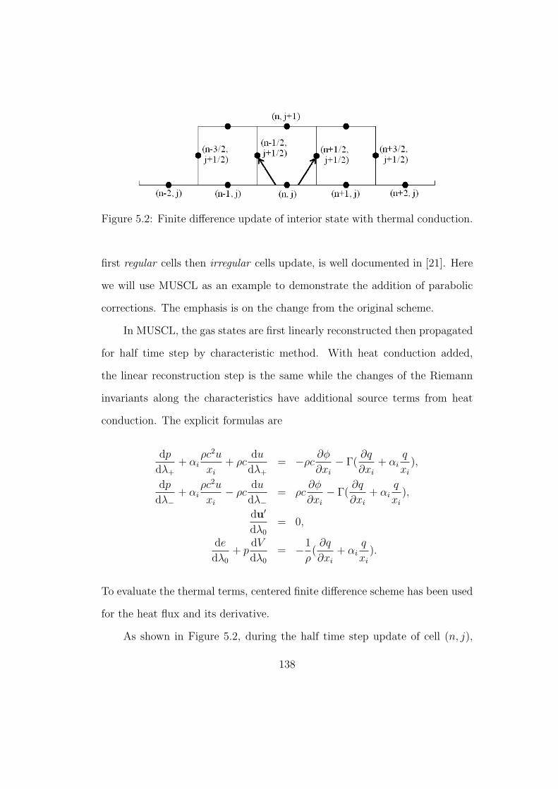
Figure 5.2: Finite difference update of interior state with thermal conduction.
first regular cells then irregular cells update, is well documented in [21]. Here
we will use MUSCL as an example to demonstrate the addition of parabolic
corrections. The emphasis is on the change from the original scheme.
In MUSCL, the gas states are first linearly reconstructed then propagated
for half time step by characteristic method. With heat conduction added,
the linear reconstruction step is the same while the changes of the Riemann
invariants along the characteristics have additional source terms from heat
conduction. The explicit formulas are
dp
dλ+
+ αiρc2u
xi
+ ρcdu
dλ+
= −ρc∂φ
∂xi
− Γ(∂q
∂xi
+ αiq
xi
),
dp
dλ−+ αi
ρc2u
xi
− ρcdu
dλ−= ρc
∂φ
∂xi
− Γ(∂q
∂xi
+ αiq
xi
),
du′
dλ0
= 0,
de
dλ0
+ pdV
dλ0
= −1
ρ(∂q
∂xi
+ αiq
xi
).
To evaluate the thermal terms, centered finite difference scheme has been used
for the heat flux and its derivative.
As shown in Figure 5.2, during the half time step update of cell (n, j),
138
the Riemann invariant along right-going characteristics to point (n + 12, j + 1
2)
and along left-going characteristics to point (n− 12, j + 1
2) both have thermal
source term proportional to
−(∂q
∂xi
+ αiq
xi
).
For medium satisfying Fourier’s Law of conductivity, q = −κ ∂T∂xi
. We need
to estimate ∂2T∂xi
2 and also ∂T∂xi
in cylindrical or spherical geometry. They are
simply given by
∂2T
∂xi2(n, j) =
T (n + 1, j)− 2T (n, j) + T (n− 1, j)
dx2,
∂T
∂xi
(n, j) =T (n + 1, j)− T (n− 1, j)
2dx,
where dx is the grid size.
After the Riemann solver step at half time step, finite volume method
is used to update the conservative quantities, namely, mass, momentum and
energy. Accordingly thermal source terms should also so added, and the terms
should be calculated using the states at half time step to guarantee 2nd order
accuracy in time. The thermal source term is nonzero only for the energy
conservation law in Eq. (4.11) and it is −( ∂q∂xi
+ αiqxi
). The heat flux and its
139
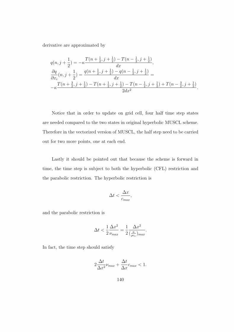
derivative are approximated by
q(n, j +1
2) = −κ
T (n + 12, j + 1
2)− T (n− 1
2, j + 1
2)
dx,
∂q
∂xi
(n, j +1
2) =
q(n + 12, j + 1
2)− q(n− 1
2, j + 1
2)
dx=
−κT (n + 3
2, j + 1
2)− T (n + 1
2, j + 1
2)− T (n− 1
2, j + 1
2) + T (n− 3
2, j + 1
2)
2dx2.
Notice that in order to update on grid cell, four half time step states
are needed compared to the two states in original hyperbolic MUSCL scheme.
Therefore in the vectorized version of MUSCL, the half step need to be carried
out for two more points, one at each end.
Lastly it should be pointed out that because the scheme is forward in
time, the time step is subject to both the hyperbolic (CFL) restriction and
the parabolic restriction. The hyperbolic restriction is
∆t <∆x
cmax
,
and the parabolic restriction is
∆t <1
2
∆x2
νmax
=1
2
∆x2
( κρcv
)max
.
In fact, the time step should satisfy
2∆t
∆x2νmax +
∆t
∆xcmax < 1.
140
5.3 Validation
5.3.1 Comparison with Analytical Solutions
First we verified the convergence of the numerical solution to the an-
alytical solution in Section 4.3.2. The temperature field is decoupled from
the hyperbolic fields. The initial conditions and parameters are given in Eqs.
(4.31) and (4.32) respectively. The numerical scheme was linearized accord-
ingly. Figure 5.3 shows the comparison of the numerical solutions of grid size
0.1 and 0.01 with the analytical solutions. The convergence is clearly verified.
We also verified the convergence of numerical solution to the analytical
solution in Section 4.4, where the hyperbolic fields are decoupled from the
temperature field. Initial conditions and parameters are the same as in Figure
4.7 except that κl = 0.01 and κr = 0.02. Figure 5.4 compares the tempera-
ture field from linearized numerical scheme with grid size 0.1 and 0.01 to the
analytical solution. The convergence is verified again.
5.3.2 Thin Thermal Layer Method
In this section we demonstrate the effect of the thin thermal layer method
in a coarse grid. To understand whether a grid is regarded as fine or coarse,
we rewrite Eq. (5.8) using the thin layer method and the linearized Clausius-
Clapeyron equation,
Ts =
κl
∆n∗lT−1 + κr
∆n∗rT1 + α√
2πRTrLdpsat
dTTsat(pv)
κl
∆n∗l+ κr
∆n∗r+ α√
2πRTrLdpsat
dT
. (5.10)
141
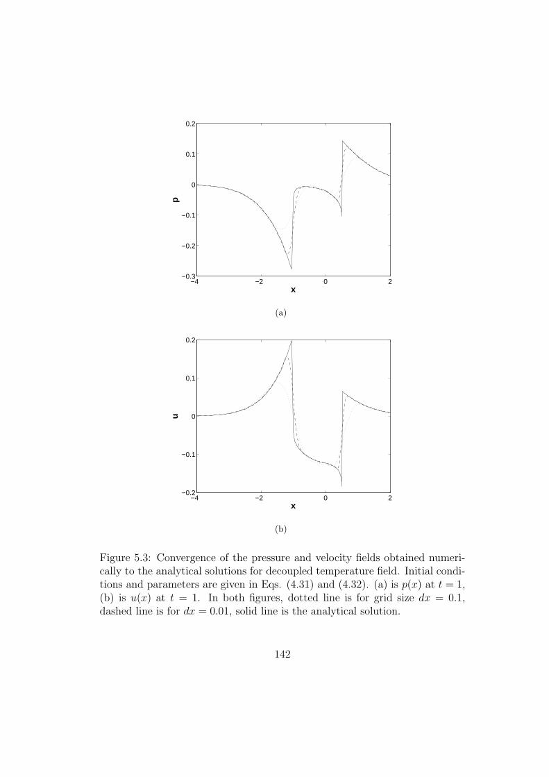
−4 −2 0 2−0.3
−0.2
−0.1
0
0.1
0.2
p
x
(a)
−4 −2 0 2−0.2
−0.1
0
0.1
0.2
u
x
(b)
Figure 5.3: Convergence of the pressure and velocity fields obtained numeri-cally to the analytical solutions for decoupled temperature field. Initial condi-tions and parameters are given in Eqs. (4.31) and (4.32). (a) is p(x) at t = 1,(b) is u(x) at t = 1. In both figures, dotted line is for grid size dx = 0.1,dashed line is for dx = 0.01, solid line is the analytical solution.
142
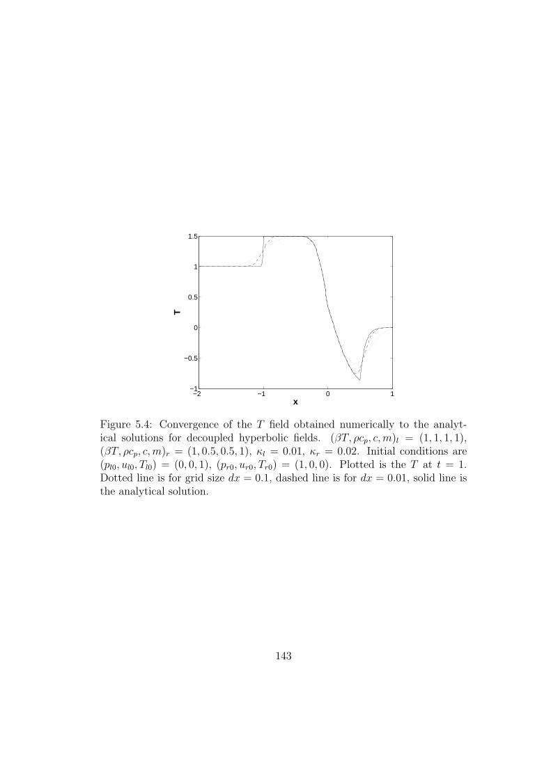
−2 −1 0 1−1
−0.5
0
0.5
1
1.5
T
x
Figure 5.4: Convergence of the T field obtained numerically to the analyt-ical solutions for decoupled hyperbolic fields. (βT, ρcp, c,m)l = (1, 1, 1, 1),(βT, ρcp, c, m)r = (1, 0.5, 0.5, 1), κl = 0.01, κr = 0.02. Initial conditions are(pl0, ul0, Tl0) = (0, 0, 1), (pr0, ur0, Tr0) = (1, 0, 0). Plotted is the T at t = 1.Dotted line is for grid size dx = 0.1, dashed line is for dx = 0.01, solid line isthe analytical solution.
143
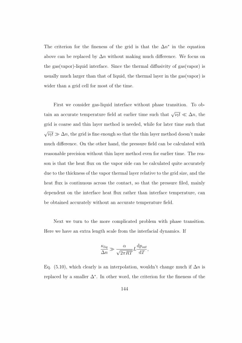
The criterion for the fineness of the grid is that the ∆n∗ in the equation
above can be replaced by ∆n without making much difference. We focus on
the gas(vapor)-liquid interface. Since the thermal diffusivity of gas(vapor) is
usually much larger than that of liquid, the thermal layer in the gas(vapor) is
wider than a grid cell for most of the time.
First we consider gas-liquid interface without phase transition. To ob-
tain an accurate temperature field at earlier time such that√
νlt ¿ ∆n, the
grid is coarse and thin layer method is needed, while for later time such that
√νlt À ∆n, the grid is fine enough so that the thin layer method doesn’t make
much difference. On the other hand, the pressure field can be calculated with
reasonable precision without thin layer method even for earlier time. The rea-
son is that the heat flux on the vapor side can be calculated quite accurately
due to the thickness of the vapor thermal layer relative to the grid size, and the
heat flux is continuous across the contact, so that the pressure filed, mainly
dependent on the interface heat flux rather than interface temperature, can
be obtained accurately without an accurate temperature field.
Next we turn to the more complicated problem with phase transition.
Here we have an extra length scale from the interfacial dynamics. If
κliq
∆nÀ α√
2πRTL
dpsat
dT,
Eq. (5.10), which clearly is an interpolation, wouldn’t change much if ∆n is
replaced by a smaller ∆∗. In other word, the criterion for the fineness of the
144
grid is
∆n ¿ κliq
√2πRT
αL
dTsat
dp.= κliq
√2πRT
TVvap
αL2.
For water at 20oC, using the thermodynamic coefficients listed in Appendix
A, the right hand side of the formula above is 4µm. If the criterion is not
satisfied, the grid is coarse for the calculation of both the temperature and
pressure fields at earlier time. The thin layer method improves the accuracy
of the simulation by a lot, as illustrated by the example below.
We consider the realistic phase transition between water and water vapor
at room temperature 20oC. The vapor is on the left side, and the EOS pa-
rameters are set as in Appendix A. Assume initially both phases are at rest,
and have the same temperature(20oC) and pressure. Initially, the vapor is
superheated by 1oC, which means
Tv − Tsat(pv) = 1oC.
The metastable liquid evaporates, which induces a couple of thermal and pres-
sure waves – the interface cools down and vapor heats up, the vapor pressure
increases, and there is a mass flux into the vapor, etc. The numerical solutions
at 5µs are plotted in Figure 5.5 and Figure 5.6. The solution from three simula-
tions are shown, namely, ∆n = 10µm, ∆n = 1µm and ∆n = 0.2µm. Recalling
the grid fineness criterion from interfacial dynamics, the case ∆n = 10µm can
be regarded as coarse grid, ∆n = 0.2µm the fine grid, while ∆n = 1µm is
intermediate. The phase boundary has moved negligible distance in 5µs.
Figure 5.5 is the numerical solution obtained without using the thin layer
145

−1 0 1−0.8
−0.4
0
0.4
0.8
T −
T0 (
oC
)
x ( cm )
(a)
−1 0 10
0.1
0.2
0.3
p −
p0 (
mba
r )
x ( cm )
(b)
−1 0 1−0.3
−0.2
−0.1
0
u (
cm
/ms
)
x ( cm )
(c)
Figure 5.5: Numerical solution to the problem with Riemann data with phasetransition between water and water vapor. Initially conditions are T0 = 20oC,Tsat(p0) = 19oC and u0 = 0, where both phases have the same T , p and u.Plotted is the solution at 5µs from direct simulation without using thin layermethod. (a) is T (x), (b) is p(x), and (c) is u(x). In all figures, the dotted curveis from the simulation with ∆n = 10µm, the dashed curve with ∆n = 1µm,and the solid curve with ∆n = 0.2µm.
146
−1 0 1−0.2
0
0.2
0.4
0.6
0.8
T −
T0 (
oC
)
x ( cm )
(a)
−1 0 10
0.1
0.2
0.3
p −
p0 (
mba
r )
x ( cm )
(b)
−1 0 1−0.3
−0.2
−0.1
0
u (
cm
/ms
)
x ( cm )
(c)
Figure 5.6: Numerical solution to the problem with Riemann data with phasetransition between water and water vapor. Initial conditions are the same asin Figure 5.5. Plotted is the solution at 5µs from direct simulation with thinlayer method. (a) is T (x), (b) is p(x), and (c) is u(x). In all figures, thedotted curve is from the simulation with ∆n = 10µm, the dashed curve with∆n = 1µm, and the solid curve with ∆n = 0.2µm.
147
method, while Figure 5.6 is obtained with thin layer method. The solid curves
(∆n = 0.2µm) have been compared with the simulation of ∆n = 0.4µm and
the convergence was verified, so we can approximately take the solid curves
to be the exact solutions to which other numerical solutions should converge.
We notice the solid curves of the corresponding temperature, pressure and
velocity fields in both figures are almost the same, which is natural since the
liquid thermal layer is thin relative to the grid only for a period much short
than 5µs. It is easy to see that the fields obtained on coarser grids in Figure
5.5 deviate severely from the exact solution, though the convergence by mesh
refinement is also clear.
As a contrast, the solutions on coarser grid shown in Figure 5.6 is almost
the same as the exact solution. The only exception to the observation above is
the liquid pressure at intermediate grid size ∆n = 1µm. It maybe argued that
the liquid pressure of the dashed line in Figure 5.5(b) is closer to the exact
solution than that in Figure 5.6(b). However, it is more like a coincidence
since the convergence of the vapor pressure is just the opposite. Increasing
the ε in Eq. (5.9) could make the liquid pressure closer to the exact solution,
but meanwhile deviate the vapor pressure from the exact value. More delicate
numerical scheme might help to resolve the issue. As a summary, the thin
thermal layer method, in spite of its crudeness, boost the accuracy of the
numerical solution at coarse grid significantly.
148
5.4 Application to One Dimensional Condensation
We used the numerical method to simulate the one dimensional conden-
sation problem. The early-stage build-up of the temperature field has been
demonstrated. The late-stage condensing flow was compared to the exact
steady states and the convergence was confirmed. The one-dimensional prob-
lem consists of a vertical tube containing a shallow layer of water with height
0.05mm. The bottom of the tube is in contact with colder material to sustain
a constant outgoing heat flux. The remaining space is filled with water vapor.
Initially the water and water vapor are at rest and in equilibrium at room
temperature – T0 = 20oC, p0 = 23.4mbar. The outgoing heat flux from water
gradually builds up a temperature gradient in the water and causes conden-
sation. For the boundary conditions at the opening of the tube, the vapor
pressure is assumed to be constant and the temperature gradient is assumed
to be zero. Mathematically, the equations for the liquid and vapor states
are the Euler equation with thermal conduction, and interface conditions is
the Rankine-Hugoniot conditions plus interfacial dynamics of phase transition
with evaporation coefficient set to 0.4. The boundary conditions are
(∂T
∂x
)
x=0
= 0,
p(x = 0) = p0,(∂T
∂x
)
x=D
= Tx0,
u(x = D) = 0,
149
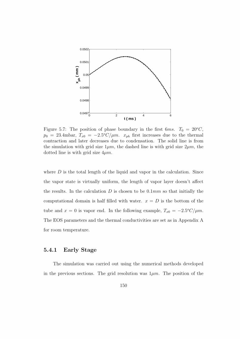
0 2 4 60.0497
0.0498
0.0499
0.05
0.0501
0.0502
x ph (
mm
)
t ( ms )
Figure 5.7: The position of phase boundary in the first 6ms. T0 = 20oC,p0 = 23.4mbar, Tx0 = −2.5oC/µm. xph first increases due to the thermalcontraction and later decreases due to condensation. The solid line is fromthe simulation with grid size 1µm, the dashed line is with grid size 2µm, thedotted line is with grid size 4µm.
where D is the total length of the liquid and vapor in the calculation. Since
the vapor state is virtually uniform, the length of vapor layer doesn’t affect
the results. In the calculation D is chosen to be 0.1mm so that initially the
computational domain is half filled with water. x = D is the bottom of the
tube and x = 0 is vapor end. In the following example, Tx0 = −2.5oC/µm.
The EOS parameters and the thermal conductivities are set as in Appendix A
for room temperature.
5.4.1 Early Stage
The simulation was carried out using the numerical methods developed
in the previous sections. The grid resolution was 1µm. The position of the
150
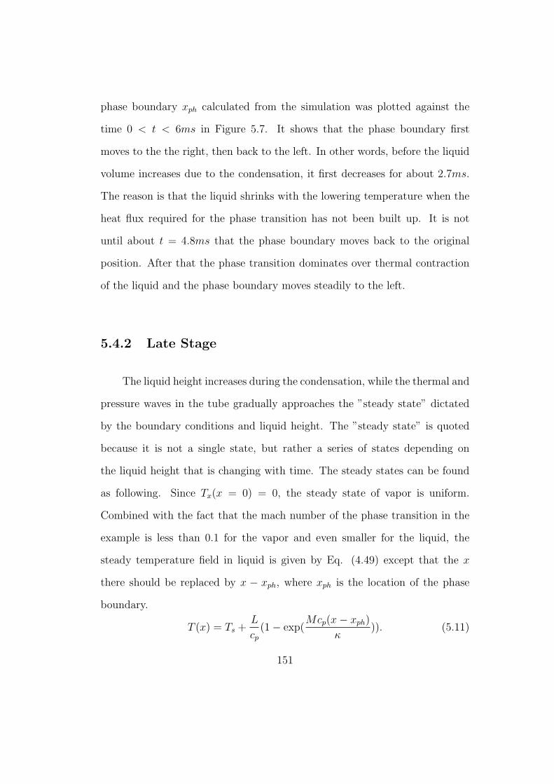
phase boundary xph calculated from the simulation was plotted against the
time 0 < t < 6ms in Figure 5.7. It shows that the phase boundary first
moves to the the right, then back to the left. In other words, before the liquid
volume increases due to the condensation, it first decreases for about 2.7ms.
The reason is that the liquid shrinks with the lowering temperature when the
heat flux required for the phase transition has not been built up. It is not
until about t = 4.8ms that the phase boundary moves back to the original
position. After that the phase transition dominates over thermal contraction
of the liquid and the phase boundary moves steadily to the left.
5.4.2 Late Stage
The liquid height increases during the condensation, while the thermal and
pressure waves in the tube gradually approaches the ”steady state” dictated
by the boundary conditions and liquid height. The ”steady state” is quoted
because it is not a single state, but rather a series of states depending on
the liquid height that is changing with time. The steady states can be found
as following. Since Tx(x = 0) = 0, the steady state of vapor is uniform.
Combined with the fact that the mach number of the phase transition in the
example is less than 0.1 for the vapor and even smaller for the liquid, the
steady temperature field in liquid is given by Eq. (4.49) except that the x
there should be replaced by x − xph, where xph is the location of the phase
boundary.
T (x) = Ts +L
cp
(1− exp(Mcp(x− xph)
κ)). (5.11)
151
At the bottom of the tube (x = D) the exponent Mcp(D − xph)/κ is about
0.2, which is small but not negligible. So ∂T∂x
is not uniform, and the transition
rate M of the steady state should be obtained by solving
(∂T
∂x
)
x=D
= −LM
κexp(
Mcp(D − xph)
κ) = Tx0.
From M the interface temperature can be found from kinetic relation with
the known vapor pressure p0. The variation of the pressure in the liquid is
negligible compared to the pressure jump at the phase boundary. The steady
state liquid pressure is given by
pl = pv + M2∆V.= p0 + M2Vv.
The liquid velocity is 0 at x = D as dictated by the boundary condition, hence
the velocity of the phase boundary is
uph = −MVl|D .= −MVl0(1 + β(T |D − T0)),
where the effect of pressure variation on density has been neglected. The vapor
velocity is
uv = MVv + uph.= MVv.
Since the phase boundary is moving, all the quantities above vary with time.
Table 5.1 is the comparison between the steady state quantities and the
corresponding ones in the evolving wave obtained from numerical simulation.
It can be seen from the table that the evolving state is closer to the steady
152
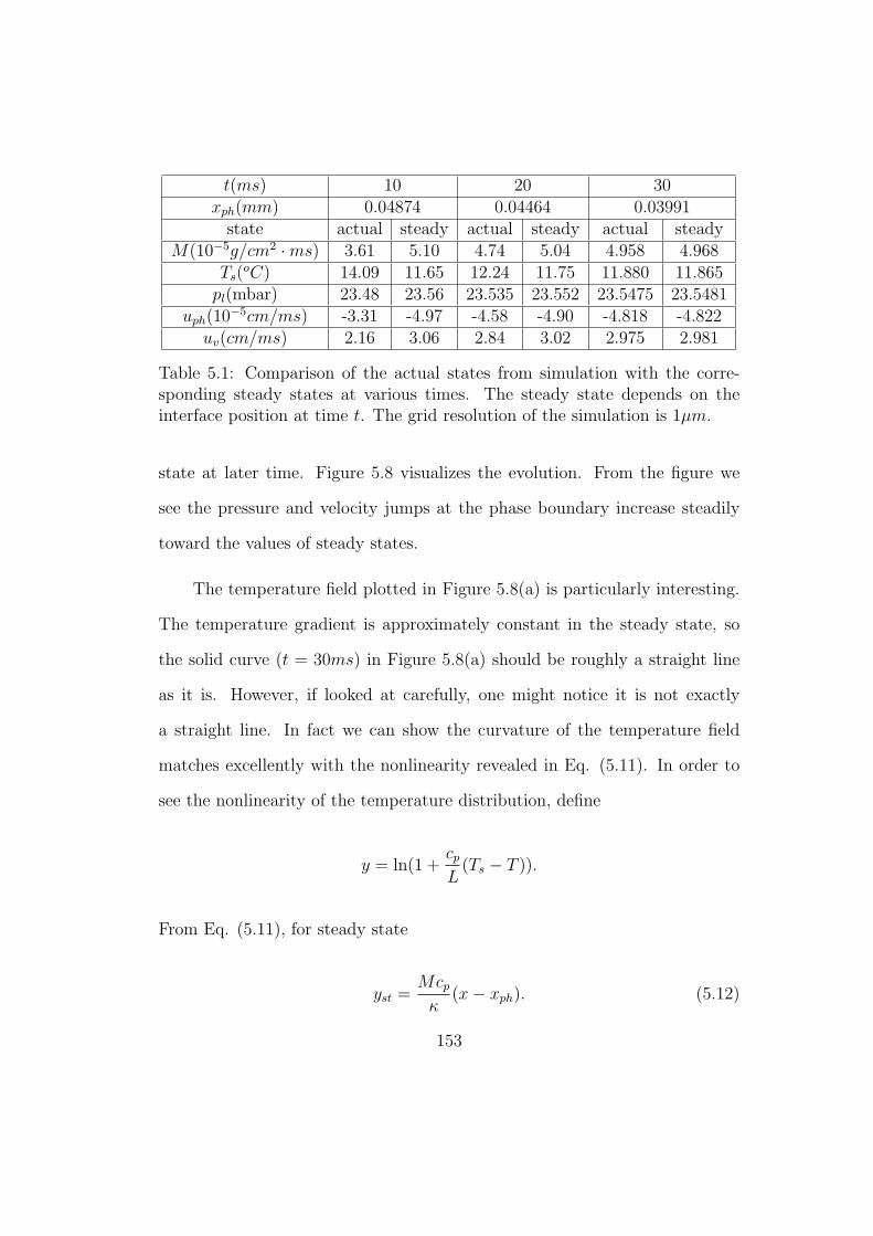
t(ms) 10 20 30xph(mm) 0.04874 0.04464 0.03991
state actual steady actual steady actual steadyM(10−5g/cm2 ·ms) 3.61 5.10 4.74 5.04 4.958 4.968
Ts(oC) 14.09 11.65 12.24 11.75 11.880 11.865
pl(mbar) 23.48 23.56 23.535 23.552 23.5475 23.5481uph(10−5cm/ms) -3.31 -4.97 -4.58 -4.90 -4.818 -4.822
uv(cm/ms) 2.16 3.06 2.84 3.02 2.975 2.981
Table 5.1: Comparison of the actual states from simulation with the corre-sponding steady states at various times. The steady state depends on theinterface position at time t. The grid resolution of the simulation is 1µm.
state at later time. Figure 5.8 visualizes the evolution. From the figure we
see the pressure and velocity jumps at the phase boundary increase steadily
toward the values of steady states.
The temperature field plotted in Figure 5.8(a) is particularly interesting.
The temperature gradient is approximately constant in the steady state, so
the solid curve (t = 30ms) in Figure 5.8(a) should be roughly a straight line
as it is. However, if looked at carefully, one might notice it is not exactly
a straight line. In fact we can show the curvature of the temperature field
matches excellently with the nonlinearity revealed in Eq. (5.11). In order to
see the nonlinearity of the temperature distribution, define
y = ln(1 +cp
L(Ts − T )).
From Eq. (5.11), for steady state
yst =Mcp
κ(x− xph). (5.12)
153
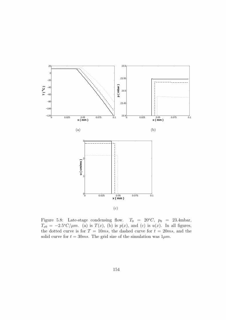
0 0.025 0.05 0.075 0.1−120
−100
−80
−60
−40
−20
0
20
T (
oC
)
x ( mm )
(a)
0 0.025 0.05 0.075 0.123.4
23.45
23.5
23.55
23.6
p (
mb
ar )
x ( mm )
(b)
0 0.025 0.05 0.075 0.10
1
2
3
u (
cm
/ms
)
x ( mm )
(c)
Figure 5.8: Late-stage condensing flow. T0 = 20oC, p0 = 23.4mbar,Tx0 = −2.5oC/µm. (a) is T (x), (b) is p(x), and (c) is u(x). In all figures,the dotted curve is for T = 10ms, the dashed curve for t = 20ms, and thesolid curve for t = 30ms. The grid size of the simulation was 1µm.
154
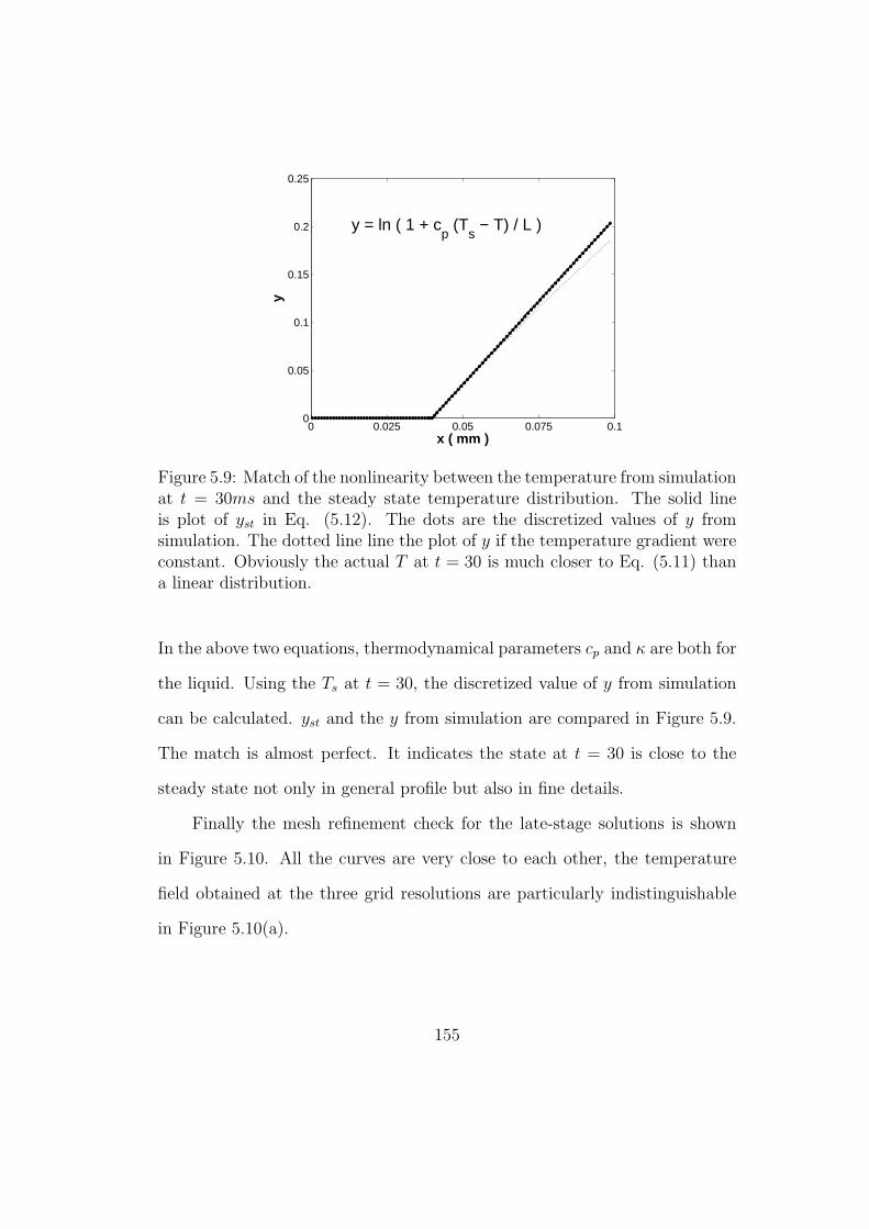
0 0.025 0.05 0.075 0.10
0.05
0.1
0.15
0.2
0.25
y
x ( mm )
y = ln ( 1 + cp (T
s − T) / L )
Figure 5.9: Match of the nonlinearity between the temperature from simulationat t = 30ms and the steady state temperature distribution. The solid lineis plot of yst in Eq. (5.12). The dots are the discretized values of y fromsimulation. The dotted line line the plot of y if the temperature gradient wereconstant. Obviously the actual T at t = 30 is much closer to Eq. (5.11) thana linear distribution.
In the above two equations, thermodynamical parameters cp and κ are both for
the liquid. Using the Ts at t = 30, the discretized value of y from simulation
can be calculated. yst and the y from simulation are compared in Figure 5.9.
The match is almost perfect. It indicates the state at t = 30 is close to the
steady state not only in general profile but also in fine details.
Finally the mesh refinement check for the late-stage solutions is shown
in Figure 5.10. All the curves are very close to each other, the temperature
field obtained at the three grid resolutions are particularly indistinguishable
in Figure 5.10(a).
155
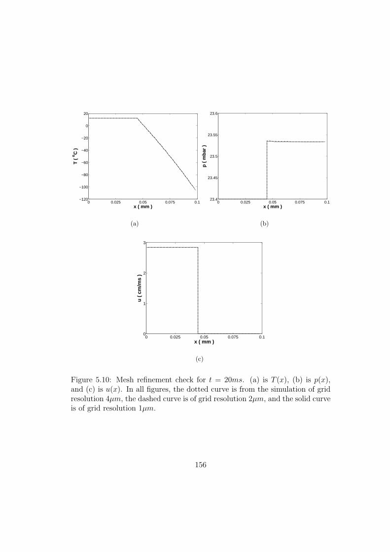
0 0.025 0.05 0.075 0.1−120
−100
−80
−60
−40
−20
0
20
T (
oC
)
x ( mm )
(a)
0 0.025 0.05 0.075 0.123.4
23.45
23.5
23.55
23.6
p (
mb
ar )
x ( mm )
(b)
0 0.025 0.05 0.075 0.10
1
2
3
u (
cm
/ms
)
x ( mm )
(c)
Figure 5.10: Mesh refinement check for t = 20ms. (a) is T (x), (b) is p(x),and (c) is u(x). In all figures, the dotted curve is from the simulation of gridresolution 4µm, the dashed curve is of grid resolution 2µm, and the solid curveis of grid resolution 1µm.
156
Chapter 6
Conclusion
6.1 DNS of Bubbly Flows and Application
Through the comparison of numerical simulations with experiments and
theoretical predictions on the propagation of acoustic and shock waves in bub-
bly fluids, the direct approach to the simulation of bubbly flows using the
method of front tracking and the FronTier code has been validated. This
method is potentially very accurate in treating many physical effects in bubbly
flows, such as drag, surface tension, viscosity, and the phase transition induced
mass transfer. It has a variety of current and prospective applications, such
as Rayleigh-Taylor instability [18, 28] and cavitating flows.
The pressure wave relaxation in bubbly mercury in the SNS target has
been investigated numerically using the FronTier hydro code. The estimation
of cavitation bubble collapse pressure under periodic ambient pressure has
been carried out systematically. The efficiency of the mitigation of overall
cavitation damage by the injection of bubbles has been calculated. The overall
cavitation damage has been found to be reduced by more than an order of
157
magnitude through the injection of gas bubbles with volume fraction of order
1%. Therefore the use of layers of non-dissolvable gas bubbles as a pressure
mitigation technique to reduce the cavitation erosion has been confirmed.
6.2 Interfacial Dynamics of Phase Transitions
The interfacial dynamics of phase transitions has been investigated along
with the case without mass flux. The rate of the non-equilibrium phase tran-
sitions is proportional to the deviation of vapor pressure from the Clausius-
Clapeyron equation. Analytical solutions to the linearized equations have been
explored. Physical spikes have been observed on the wavefronts, whose height
and width were calculated exactly for linearized equations. The spikes persist
for linearized equations but appear to vanish for nonlinear equations as time
increases. The 3-wave structure coupled to the thermal layers in the adiabatic
and isothermal limits has been clarified. The reason for the lack of a clear
wave structure in the intermediate time has also been discussed. The analyti-
cal travelling wave solutions have been found and shown to exist only on finite
domain dictated by the stability condition.
A numerical scheme for solving the Euler equations with thermal conduc-
tion and phase transitions has been implemented in the frame of front tracking.
Heat conduction has been added to the interior state update with second order
accuracy. Phase boundary propagation has been handled according to the in-
terfacial dynamics. A numerical technique has been introduced to account for
the thermal layer thinner than a grid cell. The algorithm and the thin layer
method have been validated by showing their convergence to the analytical
158

solution (or fine grid solution if analytical solution is unknown) through mesh
refinement. The scheme has also been extended to multi-dimension, adapted
to cylindrical and spherical symmetry, and applied to sample physical prob-
lems such as the simulation of boiling and cavitating processes.
159
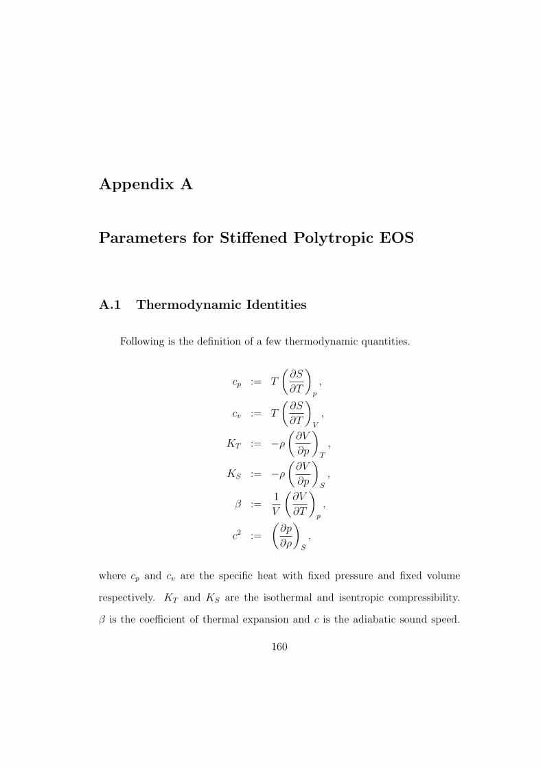
Appendix A
Parameters for Stiffened Polytropic EOS
A.1 Thermodynamic Identities
Following is the definition of a few thermodynamic quantities.
cp := T
(∂S
∂T
)
p
,
cv := T
(∂S
∂T
)
V
,
KT := −ρ
(∂V
∂p
)
T
,
KS := −ρ
(∂V
∂p
)
S
,
β :=1
V
(∂V
∂T
)
p
,
c2 :=
(∂p
∂ρ
)
S
,
where cp and cv are the specific heat with fixed pressure and fixed volume
respectively. KT and KS are the isothermal and isentropic compressibility.
β is the coefficient of thermal expansion and c is the adiabatic sound speed.
160
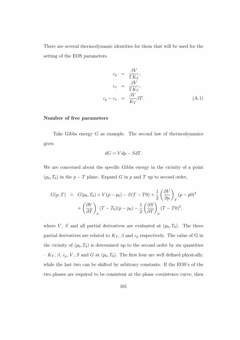
There are several thermodynamic identities for them that will be used for the
setting of the EOS parameters.
cp =βV
ΓKS
,
cv =βV
ΓKT
,
cp − cv =βV
KT
βT. (A.1)
Number of free parameters
Take Gibbs energy G as example. The second law of thermodynamics
gives
dG = V dp− SdT.
We are concerned about the specific Gibbs energy in the vicinity of a point
(p0, T0) in the p− T plane. Expand G in p and T up to second order,
G(p, T ).= G(p0, T0) + V (p− p0)− S(T − T0) +
1
2
(∂V
∂p
)
T
(p− p0)2
+
(∂V
∂T
)
p
(T − T0)(p− p0)− 1
2
(∂S
∂T
)
p
(T − T0)2,
where V , S and all partial derivatives are evaluated at (p0, T0). The three
partial derivatives are related to KT , β and cp respectively. The value of G in
the vicinity of (p0, T0) is determined up to the second order by six quantities
– KT , β, cp, V , S and G at (p0, T0). The first four are well defined physically,
while the last two can be shifted by arbitrary constants. If the EOS’s of the
two phases are required to be consistent at the phase coexistence curve, then
161
the specific Gibbs energy in both phases must be equal at the curve.
0 = ∆G = ∆E + p∆V − T∆S ⇒ ∆E = T∆S − p∆V = L− p∆V, (A.2)
where L = T∆S is the latent heat of phase transitions. Therefore, in order
for the EOS to be accurate up to the second order expansion near (p0, T0) and
consistent with phase transitions, four parameters associated with KT , β, cp,
V and one auxiliary parameter associated with L are needed. The Stiffened
Polytropic EOS introduced below has exactly five parameters to accommodate
the requirement.
As for the γ-law gas or the so-called POLY EOS implemented in FronTier,
KT = p−1, β = T−1, and the specific internal energy E has definite physical
meaning. So the five parameters reduce to two parameters, as there are in the
POLY EOS, namely, R and γ.
A.2 Liquid and Vapor EOS’s
Throughout the thesis the liquid is described by the stiffened polytropic
(SPOLY) EOS, while the vapor is considered as γ-law gas, or equivalently, the
polytropic (POLY) EOS. SPOLY EOS is a simple, analytical approximation
to an arbitrary EOS, obtained by local fitting pressure, density, temperature
and the first derivatives [36]. It has two defining equations,
p + γp∞ = (γ − 1)ρ(E + E∞),
RT = (p + p∞)V + (γ − 1)Etργ−1.
162
Other thermodynamic quantities such as entropy can be derived from them.
There are five parameters in the equations, namely, γ, R, p∞, E∞ and Et.
Since Et is usually negative, for convenience we will denote −Et by Q. And it
is easy to derive that
R = cv(γ − 1).
In the implementation, the five parameters are γ, cv, p∞, E∞ and Q. Us-
ing Eq. (A.1), it is straightforward to derive the following formulas for the
thermodynamic quantities KT , β, cp in terms of these parameters,
1
KT
= p + p∞ + (γ − 1)2QV −γ,
1
β= T +
γ
cv
QV 1−γ,
cp = cv + βRT,
or inversely, the formulas for the EOS parameters in terms of the thermody-
namic quantities KT , β, cp and V at (p, T ),
cv = cp − β2V T
KT
,
γ = 1 +βV
KT cv
,
Q = V γ−1 cv
γ
1− βT
β,
p∞ =1
KT
− (γ − 1)2QV −γ − p. (A.3)
If phase transitions are not involved, the auxiliary parameter E∞ can be
163
set arbitrarily, for example,
E∞ = E0∞ =
(p + γp∞)V
γ − 1(A.4)
to make E vanish at (p, T ). Otherwise E should satisfy Eq. (A.2), so to be
consistent with the vapor EOS,
E∞ = Eph∞ =
(p + γp∞)V
γ − 1+ L− (Ev + p(Vv − Vl)). (A.5)
The POLY EOS has two parameters γv and Rv, and the equations are
E =pV
γv − 1,
RvT = pV.
The parameters are determined by the molecular mass (Rv) and structure (γv).
A.3 Numerical Examples
A.3.1 Single liquid phase
The thermodynamic quantities and SPOLY parameters for water at 20oC
and 100oC under 1 bar pressure are listed in the following table. The units
are cm, ms, g, bar, oC and their combinations. The thermodynamic quantities
are
164
p(bar) T (oC) V (cm3/g) cp((cm/ms)2/K) k−1T (103bar) β−1(103K)
1 20 1.002 41.8 21.8 4.79
1 100 1.043 42.2 20.1 1.32
the sound speeds in the two cases are 148 and 153 (cm/ms) respectively. All
quantities can be found in standard physical and chemical handbooks. Using
Eqs. (A.3) and (A.4), the appropriate SPOLY parameters for water are
γ cv((cm/ms)2/K) p∞(103bar) Q(103bar(cm3/g)γ) E0∞(103(cm/ms)2)
1.11 41.5 19.8 168 200
1.42 37.7 15.8 25.6 55.7
A.3.2 Both phases near equilibrium
For water and water vapor near equilibrium at 20oC and 100oC, the ther-
modynamic quantities and EOS parameters are listed below. The saturation
pressure at those temperatures are 0.0234 and 1.013 bar respectively. The
thermodynamic quantities for water are virtually the same as those in the pre-
vious examples. So the only different parameter in the SPOLY EOS for water
is the E∞, which should be set to Eph∞ as in Eq. (A.5). So we will only list
the two parameters of the POLY EOS for water vapor and the Eph∞ for water.
The thermodynamic quantities are
T (oC) Psat(bar) L(103(cm/ms)2) Vv(103cm3/g)
20 0.0234 24.5 57.8
100 1.013 22.6 1.67
The EOS parameters are
165
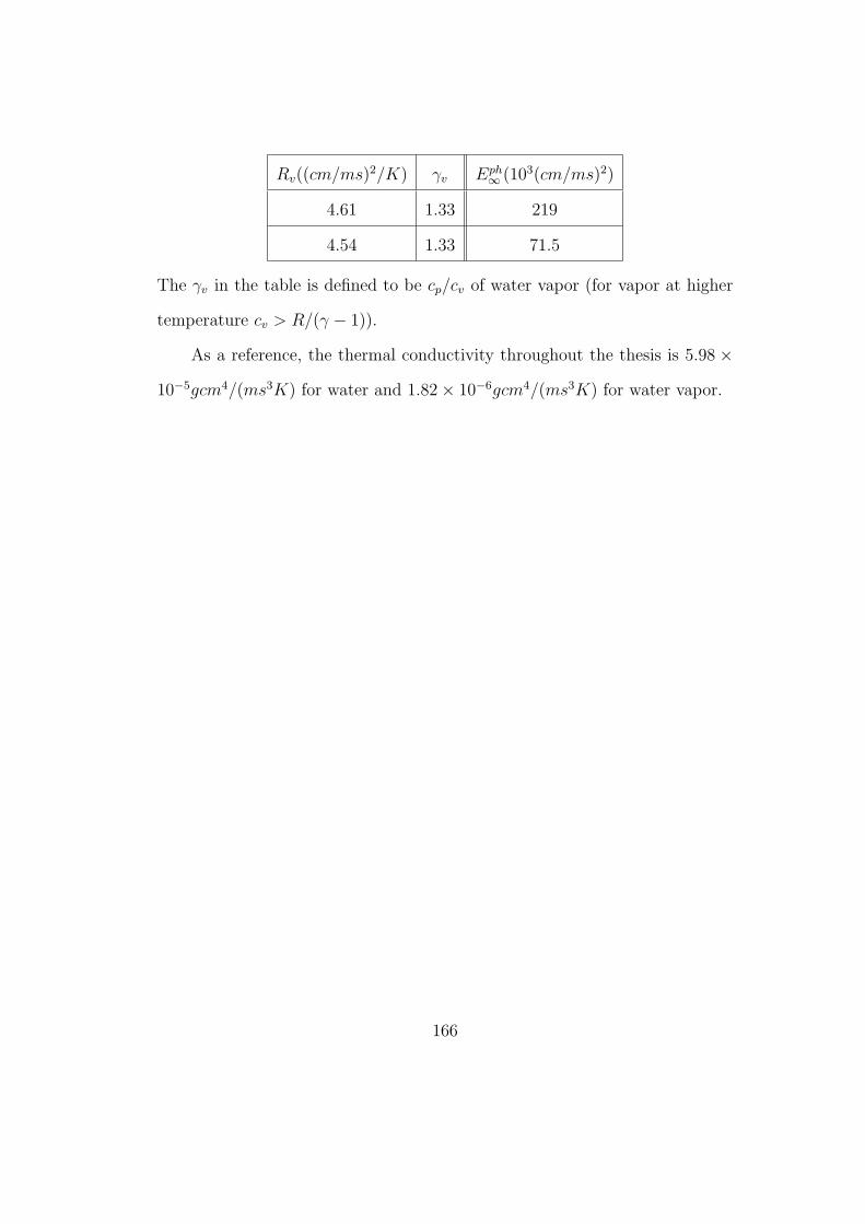
Rv((cm/ms)2/K) γv Eph∞ (103(cm/ms)2)
4.61 1.33 219
4.54 1.33 71.5
The γv in the table is defined to be cp/cv of water vapor (for vapor at higher
temperature cv > R/(γ − 1)).
As a reference, the thermal conductivity throughout the thesis is 5.98 ×10⁻⁵gcm4/(ms3K) for water and 1.82× 10⁻⁶gcm4/(ms3K) for water vapor.
166
Bibliography
[1] Status report on mercury target development and related issues. ReportNo. SNS-101060100-TR0006-R00, Spallation Neutron Source Project,July 2002.
[2] C. E. Brennen A. Preston, T. Coloius. Toward efficient computation ofheat and mass transfer effects in the continuum model for bubbly cavi-tating flows. CAV2001, session B4.002, 2001.
[3] T. Alty and C. A. Mackay. The accommodation coefficient and the evap-oration coefficient of water. Proc. R. Soc. London, Ser. A, 149:104–116,1935.
[4] A. E. Beylich and A. Gulhan. On the structure of nonlinear waves inliquids with gas bubbles. Phys. Fluids A, 2(8):1412–1428, 1990.
[5] C. E. Brennen. Cavitation and bubble dynamics. Oxford University Press,1995.
[6] R. E. Caflisch, M. J. Miksis, G. C. Papanicolaou, and L. Ting. Effec-tive equations for wave propagation in bubbly liquids. J. Fluid Mech.,153:259–273, 1985.
[7] S. L. Ceccio and C. E. Brennen. Observations of the dynamics andacoustics of travelling bubble cavitation. J. Fluid Mech., 233:633–660,1991.
[8] R. B. Chapman and M. S. Plesset. Thermal effects in the free oscillationof gas bubbles. ASME J. Basic Eng., 93:373–376, 1971.
[9] N. Chodes, J. Warner, and A. Gagin. A determination of the condensationcoefficient of water from the growth rate of small cloud droplets. J. Atmos.Sci., 31:1351, 1974.
167
[10] P. Collela. A direct eulerian muscl scheme for gas dynamics. SIAM J.Sci Stat. Comput., 6(1):104–117, 1985.
[11] P. Collela and P. Woodward. The piecewise parabolic method (ppm) forgas-dynamics. J. Comput. Phys., 54:174–201, 1984.
[12] K. W. Commander and A. Prosperetti. Linear pressure waves in bubblyliquids: Comparison between theory and experiments. J. Acoust. Soc.Am., 85(2):732–746, 1989.
[13] Y. Kuhn de Chizelle, S. L. Ceccio, and C. E. Brennen. Observations andscaling of travelling bubble cavitatio. J. Fluid Mech., 293:99–126, 1995.
[14] H. Fan and M. Slemrod. Dynamic flows with liquid/vapor phase transi-tions. In S. Friedlander and D. Serre, editors, Handbook of MathematicalFluid Dynamics, volume 1. North-Holland, 2002.
[15] R. D. Finch and E. A. Neppiras. Vapor bubble dynamics. J. Acoust. Soc.Am., 53:1402–1410, 1973.
[16] F. E. Fox, S. R. Curley, and G. S. Larson. Phase velocity and absorp-tion measurements in water containing air bubbles. J. Acoust. Soc. Am.,27(3):534–539, 1955.
[17] J. P. Garnier, Ph. Ehrhard, and Ph. Mirabel. Water droplet growth studyin a continuous flow diffusion cloud chamber. Atmos. Res., 21:41–52,1987.
[18] J. Glimm, J. Grove, X. L. Li, W. Oh, and D. H. Sharp. A critical analysisof rayleigh-taylor growth rates. J. Comput. Phys., 169:652–677, 2001.
[19] J. Glimm, J. Grove, X. L. Li, and D. C. Tan. Robust computationalalgorithms for dynamic interface tracking in three dimensions. SIAM J.Sci. Comput., 21:2240–2256, 2000.
[20] J. Glimm, J. Grove, B. Lindquist, O. A. McBryan, and G. Tryggvason.The bifurcation of tracked scalar waves. SIAM J. Sci. Statist. Comput.,9:61–79, 1988.
[21] J. Glimm, J. Grove, and Y. Zhang. Interface tracking for axisymmetricflows. SIAM J. Sci. Comput., 24(1):208–236, 2002.
168
[22] J. Glimm, M. N. Kim, X. L. Li, R. Samulyak, and Z. L. Xu. Jet simula-tion in a diesel engine. MIT Conf. on Comp. Fluid and Solid Mechanics(submitted), 2004.
[23] D. E. Hagen, J. Schmitt, M. Trueblood, J. Carstens, D. R. White, andD. J. Alofs. Condensation coefficient measurement for water in the umrcloud simulation chamber. J. Atmos. Sci., 46:803, 1989.
[24] Y. Hao and A. Prosperetti. The dynamics of vapor bubbles in acousticpressure fields. Phys. Fluids, 11(8):2008–2019, 1999.
[25] S. Hatamiya and H. Tanaka. A study on the mechanism of dropwisecondensation. Tras. Jpn. Soc. Mech. Eng. (in Japanese), 52(477B):2214,1986.
[26] R. Hickling and M. S. Plesset. Collapse and rebound of a spherical bubblein water. Phys. Fluids, 7(1):7–14, 1964.
[27] D. Y. Hsieh. Some analytical aspects of bubble dynamics. J. Basic En-gineering, 87:991–1005, 1965.
[28] H. Jin, X. F. Liu, T. Lu, B. Cheng, J. Glimm, and D.H. Sharp. Rayleigh-taylor mixing rates for compressible flow. Phys. Fluids, 17:024104, 2005.
[29] D. Juric and G. Tryggvason. Computation of boiling flows. Int. J. Mul-tiphase Flow, 24:387–410, 1998.
[30] V. Kamath and A. Prosperetti. Numerical integration methods in gas-bubble dynamics. J. Acoust. Soc. Am., 85:1538–1548, 1989.
[31] J. B. Keller and I. I. Kolodner. Damping of underwater explosion bubbleoscillations. J. Appl. Phys., 27:1152–1161, 1956.
[32] J. B. Keller and M. J. Miksis. Bubble oscillations of large amplitude. J.Acoust. Soc. Am., 68:628–633, 1980.
[33] R. Levy and M. Shearer. Kinetics and nucleation for driven thin film flow.Physica D (submitted), 2005.
[34] J. D. Macpherson. The effects of gas bubbles on sound propagation inwater. Proc. Phys. Soc. London, B70:85–92, 1957.
[35] Y. Matsumoto and F. Takemura. Influence of internal phenomena on gasbubble motion. JSME International Journal, B37:288–296, 1994.
169
[36] R. Menikoff and B. J. Plohr. The riemann problem for fluid flow of realmaterials. Reviews of Modern Physics, 61(1):75–130, 1989.
[37] M. S. Plesset and S. A. Zwick. The growth of vapor bubbles in super-heated liquids. J. Appl. Phys., 25:493–500, 1954.
[38] A. Prosperetti, L. A. Crum, and K.W. Commander. Nonlinear bubbledynamics. J. Acoust. Soc. Am., 83:502–514, 1988.
[39] A. Prosperetti and A. M. Lezzi. Bubble dynamics in a compressible liquid.part 1. first-order theory. J. Fluid Mech., 168:457–478, 1986.
[40] A. Prosperetti and M. S. Plesset. Vapor bubble growth in a superheatedliquid. J. Fluid Mech., 85:349–368, 1978.
[41] Lord Rayleigh. On the pressure developed in a liquid during the collapseof a spherical cavity. Phil Mag., 34:94–98, 1917.
[42] E. Silberman. Sound velocity and attenuation in bubbly mixtures mea-sured in standing wave tubes. J. Acoust. Soc. Am., 29(8):925–933, 1957.
[43] Z. H. Teng, A. J. Chorin, and T. P. Liu. Riemann problems for reactinggas, with applications to transition. SIAM J. Appl. Math, 42(5):964–981,1982.
[44] M. Watanabe and A. Prosperetti. Shock waves in dilute bubbly liquids.J. Fluid Mech., 274:349–381, 1994.
[45] S. W. Welch. Local simulation of two-phase flows includind interfacetracking with mass transfer. J. Comp. Phys., 121:142–154, 1995.
[46] L. Van Wijngaarden. One-dimensional flow of liquids containing smallgas bubbles. Ann. Rev. Fluid Mech., 4:369–396, 1972.
170