direct correlation functions and the density functional theory of polar solvents

www.elsevier.com/locate/chemphys

Chemical Physics 319 (2005) 261–272

Direct correlation functions and the density functional theoryof polar solvents

Rosa Ramirez a,1, Michel Mareschal a,2, Daniel Borgis b,*

a CECAM, Ecole Normale Superieure de Lyon, 69364 Lyon, Franceb Modelisation des Systemes Moleculaires Complexes and LAE UMR-CNRS 8587, Universite Evry-Val-dEssonne, 91405 Evry, France

Received 14 January 2005; accepted 6 July 2005Available online 19 September 2005

Abstract

To describe the solvation properties of polar or charged species, and the reaction free-energy of charge transfers, we propose ageneralization of the Marcus electrostatic polarization free-energy functional which accounts for the molecular nature of the solvent.The proposed generic free energy functional relies crucially on the knowledge of the direct correlation function of the homogeneoussolvent. For the case of a dipolar solvent, we show how this fundamental quantity can be extracted directly from molecular dynam-ics simulations of the pure solvent instead of the traditional route of integral equation theories. The direct correlation function com-puted from simulation is compared to approximate ones obtained from linearized and quadratic HNC integral closures. Theperformance of the corresponding density functionals is assessed, in comparison to ‘‘exact’’ molecular dynamics results, for the sol-vation free-energies and the solvent density profiles around simple molecular solutes. 2005 Elsevier B.V. All rights reserved.

Keywords: Solvation free-energy; Density functional theory; Integral equations

1. Introduction

Most of our vision of charge transfer processes insolution comes from the Marcus–Levich–Dogonadzeelectron transfer theory based on a dielectric continuumdescription of the solvent [1,2]. This approach has beenextended in many aspects, and applied to the study of anumber of electron and proton transfer reactions inPhysics, Chemistry, and Biology by Kuznetsov and hiscollaborators [3,4]. In the original Marcus view [1], thesolvent is described by a non-equilibrium polarizationfield obeying a quadratic free-energy functional (the

0301-0104/$ - see front matter 2005 Elsevier B.V. All rights reserved.

doi:10.1016/j.chemphys.2005.07.038

* Corresponding author. Tel.: +33 1 69 47 01 40; fax: +33 1 69 47 0146.

E-mail address: [email protected] (D. Borgis).1 Present address: UMR-CNRS 8587, Universite Evry-Val-dEss-

onne, 91405 Evry, France.2 Present address: Universite Libre de Bruxelles, Faculte des

Sciences, 1050 Bruxelles, Belgium.

so-called Marcus functional [5]). The subsequent gener-alization of the Marcus–Levich–Dogonadze theory be-yond continuum electrostatics has gone in twocomplementary direction. A mainly ‘‘computational’’route, pioneered by Warshel [6] and applied to manychemical or biochemical electron and proton transferprocesses ever since [7–11], consists in adopting a fullyatomistic description of the charge transfer system andusing molecular simulations to characterize the chargetransfer energetics, including reaction free-energy andsolvent reorganization free-energy. Although the Gauss-ian property of the electrostatic energy gap fluctuations,postulated in Marcus theory, could be verified also at amicroscopic level and can be used to simplify the calcu-lations and provide approximate values, the precisecomputation of the reaction free-energies requires exten-sive simulations relying on thermodynamic integrationtechniques [12]. A more ’’analytical’’ consists in general-izing the Marcus electrostatic functional to account for

mailto:[email protected]

262 R. Ramirez et al. / Chemical Physics 319 (2005) 261–272

finer microscopic effects, in particular, the non-local (ork-dependent) character of the static dielectric constant.There have been a number of theoretical works devotedto the study of the static dielectric constant (k) of polarfluids (including longitudinal and transverse compo-nents), of the corresponding frequency-dependent quan-tity (k,x), and of the implication of those microscopicquantities for the energetics and dynamics of chargetransfer processes [13–24]. For realistic solvents, (k,x)can be extracted from molecular simulations. Such cal-culations were performed by Fonseca et al. for methanol[25,26] and Bopp et al. for water [27,28].

In previous works [29,30] we have proposed a gener-alization of the Marcus polarization density functionalbased on the classical density functional theory ofmolecular fluids that accounts for the molecular natureof the solvent. In this description, the solvent is com-posed of rigid molecules described by their position r

and orientation X and it is subjected to an external fieldproduced by a solvated molecule. We have proved that areasonable approximation is to consider the inhomoge-neous solvent characterized by only two macroscopicfields: the number density n(r) and the polarizationP(r). In this case, the Gibbs free energy functional de-pends exclusively on these two fields G G[n,P], andit has a minimum at the equilibrium density ne(r) andpolarization Pe(r). With respect to the Marcus polariza-tion functional, or the connected Gaussian polarizationfield approach of Song et al. [31,32], the proposed func-tional does include additional microscopic effects suchas the coupling of polarization density to solvent den-sity, the dipolar saturation, and the non-local characterof the dielectric constant evoked above. The recentextension by Matyushov [18] of the Song–ChandlerGaussian field theory to the solvent reorganization en-ergy of electron transfer reactions does include the lattereffect but not the two former. Our functional approachhas also connections with the density functional theoryof nonuniform polyatomic fluids developed by Chandleret al. [33,34], although in our case the internal structureof the solvent is accounted for by the definition of amolecular dipole (and, beyond that, of molecular multi-poles) rather than by distributed interaction sites.

The rigorous definition of our generic dipolar solventfunctional involves the space and orientation dependentdirect correlation function (c-function, c(1,2)) of theinhomogeneous solvent which is connected to the paircorrelation function (h-function, h(1,2)) through theOrnstein–Zernike (O–Z) equation. A valuable approxi-mation that we explored recently consists in replacingthe inhomogeneous direct correlation function by thatof the homogeneous solvent (in the absence of any sol-ute). The problem is thus cast into the a priori definitionof that quantity (or its various orientational projec-tions). This has to be done once for good for a given sol-vent and given thermodynamic conditions. The resulting

functional can be applied then to study the solvationproperties of any solute.

The direct correlation function of a molecular liquidcan be inferred by different ways. An approximate ap-proach is to use integral equation theories, with MSA[35,40,41] or HNC [36,51] closures. A method whichcan be qualified as ‘‘exact’’ for a given molecular model,and follows the spirit of the work of Kornishev and col-laborators [27,28] for the k-dependent dielectric con-stant, is to use computer simulations to calculate theexact pair correlation function h(1,2) and subsequentlyinvert the O–Z equation to get the exact c(1,2). This isthe approach proposed in [29] and developed in moretechnical details here. This will be done for a modeldipolar solvent, the so-called Stockmayer fluid, gov-erned by only Lennard–Jones and dipolar interactions,adjusted to yield a few characteristic properties of waterin term of particle size, density, dielectric constant, andpossibly surface tension. The model goes well beyond acontinuum dielectric description but it is still away fromreal water since it does not include H-bonding. TheStockmayer fluid has been widely studied both theoret-ically and simulationally (see for example [44] for a re-view). The h-projections have been calculated fromsimulations [38] as well as from multiple approximationsof the HNC theory [51] but the c-projections have notdeserved the same attention, probably because their util-ity was not established. The main part of this article isthen dedicated to the method to extract the direct corre-lation function from MD simulations of the homoge-neous solvent.

The computation of direct correlation functions fromsimulation is reputed as a numerically difficult problem.The noisy tails in the h-function computed in Monte-Carlo or molecular dynamics (MD) simulations makedifficult the inversion of the O–Z equation in Fourierspace. Some extrapolation methods have been proposedto solve this problem [50]. Our approach is slightly dif-ferent. In the case of the Stockmayer fluid, whenc(1,2) and h(1,2) are expressed in the basis of rotationalinvariants, the O–Z relation can be written as a set ofuncoupled equations in terms of short-ranged functions[40,41,45,47]. We will use this result to justify the use ofthe Baxters relation [39], instead of O–Z relation. This isthe same idea prevailing in the MSA solution for dipolarhard spheres [47] except that we are not imposing MSAconditions. We extract the c-projections in real spacewith the minimization method proposed by Dixon andHutchinson [37]. This method has been rarely used[42] but it leads to well converging and reliable correla-tion functions. Besides, we will show that, for the case ofpolar fluids, the calculation of the c-projections does notrequire extensive MD simulations. A cubic simulationbox with a side of 10 diameters and simulations of afew nanoseconds are enough to collect enough statisticsand find the proper projections.

R. Ramirez et al. / Chemical Physics 319 (2005) 261–272 263

This article is organized as follows. Section 2 intro-duces the theoretical background for the direct correla-tion function of a molecular liquid and its relation todensity functional theory. Section 3 is a reminder ofthe O–Z relation and the transformations needed to re-write it as Baxters relation. We also make a brief intro-duction to the minimization method of Dixon andHutchinson. In Section 4, we discuss the numerical pro-cedure to extract the c-projections from MD simulationsand we compare them with the ones computed from thelinearized (LHNC) and quadratic (QHNC) approxima-tions of the hypernetted chain theory. In Section 5, wecompare the density and orientational profiles of theStockmayer fluid around a spherical ion obtained byDFT minimization at various levels of theory or by di-rect MD simulations. The DFT/MD comparison is alsomade for an organic molecule, N-methylacetamide. Thismolecule presents two isomeric forms for which thereaction free energy can be estimated and compared. Fi-nally, we draw conclusions in Section 6.

2. Theoretical background

2.1. h- and c-Functions and the Ornstein–Zernicke

equation

We consider here a Stockmayer fluid composed of ri-gid spherical particles interacting through the potential

uð1; 2Þ ¼ uLJðr12Þ þ uddðr12;X1;X2Þ; ð1Þwhere uLJ(r12) is the Lennard–Jones potential, andudd(r12,X1,X2) is the dipole–dipole interaction definedas

uddðr12;X1;X2Þ ¼ l20

4p0r12U112ð1; 2Þ ð2Þ

with l0 the dipolar moment of the particle and 0 thevacuum permittivity. The function U112(1,2) is defined as

U112ð1; 2Þ ¼ ½3ðX1 s12ÞðX2 s12Þ X1 X2; ð3Þwhere Xi is the unitary vector in the direction of thedipolar moment of particle i in the laboratory frame,and s12 = r12/r12 is the unitary vector in the directionof the vector joining the centers of the two particles.

For an homogeneous solvent the correlation functionh(1,2) can be formally expressed as an infinite expansionin a basis of rotational invariants [41]. It has been shown[45,47] that, for the case of a purely dipolar fluid, a rea-sonable description is obtained with only three invari-ants U000(1,2) = 1, U110(1,2) = X1 Æ X2 and U112(1,2)defined in Eq. (3). The pair correlation functions readsin this basis

hð1; 2Þ ¼ h000ðr12Þ þ h110ðr12ÞU110ð1; 2Þþ h112ðr12ÞU112ð1; 2Þ. ð4Þ

The projections of h(1,2) are defined as

h000ðr12Þ ¼ hð1; 2Þh iX1;X2

h110ðr12Þ ¼ 3 U110ð1; 2Þhð1; 2Þh iu1;X2

h112ðr12Þ ¼3

2U112ð1; 2Þhð1; 2Þh iX1;X2

ð5Þ

where hiX1;X2denotes the average over all possible orien-

tations X1 and X2.We are using the standard Wertheims normalization

for the rotational invariants [47]. The normalizationsuggested by Blum [40] is a more suitable choice whenworking with more complex interacting potentials, andit permits to follow step by step Blums mathematicalderivation of the O–Z relations for the projections inthe basis of invariants. The mathematical formalism forour simple fluid model is not as much involved and thuswe have preferred to keep the normalization that is morewidely used.

The direct correlation function c(1,2) is related withh(1,2) through the O–Z relation

hð1; 2Þ ¼ cð1; 2Þ þ n0

Zhð1; 3Þcð1; 3Þ dr3

X3

. ð6Þ

This relation is closed if c(1,2) is written in terms of thethree same invariants as h(1,2), namely

cð1; 2Þ ¼ c000ðr12Þ þ c110ðr12ÞU110ð1; 2Þþ c112ðr12ÞU112ð1; 2Þ. ð7Þ

2.2. A generic density functional for dipolar fluids

Now consider a homogeneous (Stockmayer) solventwith number density n0 = N/V, zero polarization andGibbs free energy G0 = G[n0,0]. A solvated molecule willcreate a field in the solvent producing an inhomogeneousdensity and polarization n0 ! n(r) and P = 0 ! P(r),with the corresponding change in free energy. Thefunctional DG[n,P] = G[n,P] G[n0,0] has a minimumat the equilibrium densities ne(r), Pe(r) and its value atthe minimum is the difference in free energy betweenthe inhomogeneous and homogeneous solvents, i.e., thesolvation energy.

In [29,30], we have derived a generic expression ofG[n,P], which can be split into three contributions: anideal part, an excess part and an external part describingthe interaction with the solute

DG½n;P ¼ DGid½n;P þ DGexc½n;P þ DGext½n;P ð8Þwith expressions

DGid½n;P ¼Z

drnðrÞ lnðnðrÞn0

Þ nðrÞ þ n0

þZ

drPðrÞL1 PðrÞ=nðrÞ½

Z

drnðrÞ lnsinh L1 PðrÞ=nðrÞ½

L1 PðrÞ=nðrÞ½

" #; ð9Þ


DGexc½n;P ¼ 1

2

Zdr nðrÞ n0ð Þ/excðrÞ þEexcðrÞ PðrÞ½ ;

ð10Þ

DGext½n;P ¼ bZ

dr nðrÞ/extðrÞ þEextðrÞ PðrÞ½ . ð11Þ

L1ðxÞ is the inverse of the Langevin function.The equilibrium condition is written as

dDG½n; P dn

n;Pequil

¼ 0;dDG½n; P

dP

n;Pequil

¼ 0.

The excess potential and electric fields appearing in (10)depend on the various projections of the direct correla-tion function of the homogeneous solvent defined in Eq.(7), i.e., c000(r12), c110(r12) and c112(r12):

/excðr1Þ ¼Z

dr2c000ðr12Þ nðr2Þ n0ð Þ;

Eexcðr1Þ ¼Z

dr2Pðr2Þ c110ðr12Þ c112ðr12Þð Þ

þZ

dr2r12ðPðr2Þ r12Þc112ðr12Þ.

ð12Þ

Provided we know these projections, the functional (8)can be minimized to obtain the equilibrium number den-sity and polarization. The evaluation of DG[n,P] at theequilibrium is the solvation free energy.

Ref. [30] gives the conditions under which the generalfunctional can be reduced to the electrostatic polariza-tion functional ofMarcus theory. This general functionalthus requires as microscopic input the direct correlationfunction of the homogeneous fluid. Concerning thispoint, two different approaches can be considered.

(i) A number of projections in the basis of rotationalinvariants of the function h(1,2) = g(1,2) 1 canbe computed in MD simulations of the homoge-neous solvent. The inversion of the Ornstein–Zer-nike (O–Z) equation leads to the requiredprojections of c(1,2).

(ii) An approximation of the required projections ofc(1,2) can be found theoretically using the Orn-stein–Zernike (O–Z) relation together with a clo-sure relation, for example one of the versions ofthe hypernetted-chain (HNC) theory.

Those two approaches will be compared in Section 4.

3. Inverting the Ornstein–Zernike equation

3.1. The Baxter equation

Inserting the expressions (4) and (7) into (6) and tak-ing the Fourier transform we find the closed set of equa-tions [45,47,49]

h000ðkÞ ¼ c000ðkÞ þ n0h000ðkÞc000ðkÞ; ð13Þ

h110ðkÞ ¼ c110ðkÞ þn03

h110ðkÞc110ðkÞ þ 2h112ðkÞc112ðkÞh i

;

ð14Þ

h112ðkÞ ¼ c112ðkÞ þn03

h110ðkÞc112ðkÞ þ h112ðkÞc110ðkÞh

þh112ðkÞc112ðkÞi; ð15Þ

where hðkÞ denotes Fourier transforms, and h112ðkÞ de-notes the Hankel transform of h112(r),

h112ðkÞ ¼ 4pZ 1

0

j2ðkrÞh112ðrÞr2 dr. ð16Þ

The Hankel transform of c112(r) (or h112(r)) can be for-mally written as the Fourier transform of the functioncð0Þ112ðrÞ (or h

ð0Þ112ðrÞ) defined by

cð0Þ112ðrÞ ¼ c112ðrÞ 3

Z 1

r

c112ðsÞs

ds; ð17Þ

c112ðrÞ ¼ cð0Þ112ðrÞ 3

r3

Z r

0

cð0Þ112ðsÞs2 ds. ð18Þ

The same relations apply to h112(r) and hð0Þ112ðrÞ.We now apply what is frequently called a v-transfor-

mation [40,41]. This is a linear combination of theprojections,

CSðrÞ ¼ c000ðrÞ;

CþðrÞ ¼1

3c110ðrÞ þ 2cð0Þ112ðrÞh i

;

CðrÞ ¼1

3c110ðrÞ cð0Þ112ðrÞh i ð19Þ

and the equivalent transformations of h000(r), h110(r) andhð0Þ112ðrÞ. This transformation allows to rewrite Eqs. (13)–(15) as a set of uncoupled equations,

H vðkÞ ¼ CvðkÞ þ n0H vðkÞCvðkÞ ð20Þwith v = S, + or . In direct space, any of these equa-tions corresponds to

H vðrÞ ¼ CvðrÞ þ n0

ZH vðr0ÞH vðj r r0 jÞ dr0. ð21Þ

This equation is easily recognizable as the O–Z equationfor an isotropic, homogeneous system composed of par-ticles interacting through a spherical symmetricalpotential.

Any of the functions Cv(r) is a short ranged function.Note that if we consider that the asymptotic behavior ofthe direct correlation function is given by the interactionpotential,

cð1; 2 !r12!1 buð1; 2Þ;then the function cð0Þ112ðrÞ is zero for r > R112. The samefeature applies to c000(r). Assuming it decays as 1/r6

[45], we can postulate that it is negligible from some dis-tance R000 on. We can also expect c110(r) to vanish at


some distance R110 since there is no long range potentialhaving a component on this element of the basis. As thefunctions C+(r) and C(r) are linear combinations ofc110(r) and c112(r), we can state that any function Cv(r)(with v = S, + or ) is either strictly zero or negligibleat some distance Rv.

For simplicity we will drop the sub index v from nowon, having in mind that any of the following relationsapply to any of the v-functions. Assuming that a func-tion C(r) vanishes from r > R, Baxter transformed equa-tion (21) into the pair of equations [39],

rHðrÞ ¼ Q0ðrÞ þ 2pn0

Z R

0

dsðr sÞHðj r s jÞQðsÞ; r > 0;

ð22Þ

rCðrÞ ¼ Q0ðrÞ þ 2pn0

Z R

rdsðr sÞQ0ðsÞQðs rÞ; r < R;

ð23Þ

where Q(r) is an auxiliary function, continuous at r = R

and such that Q(r) = 0 for r P R. Q 0(r) stands for thederivative dQ/dr, so that

QðrÞ ¼ Z R

rQ0ðsÞ ds. ð24Þ

For a function H(r) known for r 6 R, the relation (22)results in an integral equation for Q 0 that can be solvednumerically. Once Q 0(r) known, the calculation of C(r)from Eq. (23) is straightforward, provided an extra rela-tion for C(r = 0). This relation can be obtained by differ-entiating Eqs. (22) and (23), subtracting, and allowingr ! 0 [43], which leads to

Cð0Þ Hð0Þ ¼ 2pn0

Z R

0

drðrHðrÞQ0ðrÞ Q0ðrÞQðrÞÞ

Q0ð0ÞQð0Þ. ð25Þ

Because of the factor r on the left of Eq. (23), the numer-ical procedure appears highly inaccurate for very smallvalues of r. To avoid this problem, these values are ob-tained by interpolation.

A further question remains of choosing the appropri-ate cut-off distance R. As pointed out in [37], arbitrary R

values do not necessarily preserve the continuity of H(r)(and therefore of C(r)) at r = R. This requirement is ful-filled if Q 0(R) = 0 or, at worst, (Q 0(R)/R)2 is minimum.There exist several possible cut-off R values satisfyingthis condition, but not all of them will lead to the correctasymptotic behavior of c(1,2).

3.2. The method of Dixon and Hutchinson

Dixon and Hutchinson [37] proposed a variationalmethod for solving the Eq. (22) for Q

0(r) which avoids

possible inaccuracies at small r values. The basic idea

is to construct a dimensionless objective functionalFðQ0Þ that presents a minimum for the function Q 0(r)which is solution of Eq. (22).

The first step is to rewrite Eq. (22) as

rHðrÞ ¼ Q0ðrÞ 2pn0

Z R

0

dsQ0ðsÞKðr; sÞ; r > 0 ð26Þ

with a kernel K(r, s) equals to

Kðr; sÞ ¼Z r

0

dppHðpÞ Z jrsj

0

dppHðpÞ. ð27Þ

Rearranging Eq. (26), the function

AðrÞ ¼ HðrÞ þ Q0ðrÞr

þ 2pn0r

Z R

0

dsQ0ðsÞKðr; sÞ ð28Þ

is defined for r 5 0. To account for the behavior of Eqs.(22) and (23) at r = 0, the constants B, C and D are de-fined as

B ¼ 1

r4

Z R

0

dsQðsÞ½Q0ðsÞ þ sHðsÞ; ð29Þ

C ¼ 1

rQ0ð0Þ þ 2pn0

Z R

0

ds sQðsÞHðsÞ

; ð30Þ

D ¼ 1

rQ0ð0Þ 2pn0

Z R

0

dsQ0ðsÞQðsÞ

. ð31Þ

As remarked in [42], beware of the misprints in the ori-ginal article [37] concerning these expressions. All theseterms should vanish for the proper Q 0(r). Discretizing toM points equally spaced between 0 < r < R, and takingr = i R/M, with i = 0 . . .,M, the function FðQ0Þ is writ-ten as

F ¼ B2 þ C2 þ D2 þXMi¼1

A2i . ð32Þ

Minimization of F with respect to Q0i leads to the linear

system

oF

oQ0i

¼XMj¼0

aijQ0j þ bj ¼ 0; i ¼ 0; . . . ;M . ð33Þ

The coefficients aij and bj are functions of Q, so that thesolution is found through an iterative process.

The zeros in Q 0(r) are candidates for being the cut-offradii R of the function C(r). As will be shown, there aremore than one possible R values although not all ofthem will lead to the correct asymptotic behavior ofc(1,2).

4. Computation of the c-projections

All the direct correlation functions discussed in thissection have been calculated using the Dixon–Hutchin-son minimization procedure described above to invertthe O–Z equations.

0 1 2 3 4 5 6 7 8 9

-4

-3

-2

-1

0

1

2

3

4

5

6

7

Q'(r

)

r (A)

5 6 7 8-0.3

-0.2

-0.1

0.0

0.1

r(A)

Q'(r

)

Fig. 1. Baxters auxiliary functions Q0SðrÞ (solid line), Q0

þðrÞ (dashedline) and Q0

ðrÞ (dotted line). In the inset, the oscillatory behavior atr 2r.

0 1 2 3 4 5 6 7 8-18

-16

-14

-12

-10

-8

-6

-4

-2

0

2

c 000(

r)

r (A)

3 4 5 6 7 8 9 10 11 12-0.5

0.0

0.5

1.0

1.5

2.0

r(A)

c 000(r

)

Fig. 2. The function c000(r) extracted from simulations with R = 1.65(dash-dotted line), R = 2.12r (solid line), R = 2.8r (dashed line) andR = 3.5r (dotted line). All those curves are virtually identical on thescale of the figure. Differences appear more clearly in the inset, wherethe asymptotic behavior of the functions is shown together with thevan der Waals part of the potential 4LJb(r/r)

6 (solid upper line).


A uniform discretization of F into M = R/d points,with d = 0.02 A, was employed. No smoothing of the in-put functions H(r) was done, and the extra valuesneeded to perform the calculations were obtained witha cubic spline fit. The computation of the minimum ofF was done with a conjugate gradient minimizationalgorithm. The convergence limit for F was set to 106

or 300 iterations. In the worst cases we got F 6 103.We used a set of cut-off trial radii ranging from 2 A(smaller than r) to 4r 12 A, spaced by 0.5 A. For a gi-ven trial cut-off Rt the value Q

0(r) at the cut-off Rt1 wasused as initial condition in order to reduce the numberof iterations.

4.1. The c-projections extracted from MD simulations

We performed MD simulations of a system com-posed of N = 2916 Stockmayer particles, with densityn0 = 0.0289 at T = 298 K, in a cubic box of size46.2 A. The parameters for the interaction potentialsare: r = 3.024 A, LJ = 1.847 kJ/mol and l0 = 1.835 D.These quantities correspond to the set of reducedvariables: n* = nr3 = 0.8, T* = kBT/LJ = 1.35 andl*

2 = l0/kBTr3 = 2.96. A similar set of parameters

was studied by Pollock and Alder [38]. The model yieldsa dielectric constant close to that of water (80).

The MDMULP program from the CCP5 program li-brary [46] was used for the MD simulations. In this pro-gram, the Ewald sum for point dipoles is implemented tocompute the forces from the electrostatic interactions.The functions h000(r), h110(r) and h112(r) were computedaccording to Eq. (5) up to a distance of L = 23 A. See[29]. The functions H0(r), H+(r) and H(r) were calcu-lated from the relations (19). For each of these func-tions, the functional F was minimized in order to findthe zeros of Q 0(r).

In Fig. 1, the function Q0SðrÞ;Q0

þðrÞ and Q0ðrÞ are

presented. The first thing to be observed is that Q 0(r)is linear up to a distance r r. This is the behavior pre-dicted in the MSA theory of dipolar hard spheres [47].At this distance, there is always a zero or a discontinu-ity. This zero is the result of the discontinuous derivativein the h-projections; the c-projections evaluated with thiscut-off do not present the expected asymptotic behavior.Then, it must be concluded that R = r is not a possiblecut-off for the functions C(r). The existence of the zerosof Q 0(r) has not been proved mathematically, but it hasbeen verified numerically for the case of a fluid com-posed of hard spheres and Lennard–Jones particles[37,42]. In our case, we do find oscillations around zerobut quite locally and at distances around 2r. See the in-set of Fig. 1. In order to get these curves we minimized F

using trial Rt distances every 0.1 A to enforce a betterconvergence.

The possible cut-off radius for CS(r) (or c000(r)) areRS = 1.65r, 1.75r and 2.12r (corresponding to 5, 5.3

and 6.4 A). From this distance on, no zeros are ob-served. In [42] the lack of oscillations beyond similar dis-tances is attributed to an inaccurate sampling of h000(r)close to the simulation-box boundaries. We do not be-lieve that this is the case here since 2.12r is quite smallcompared to our simulation box.

The calculated c000(r) projection is not very sensitiveto the R chosen as cut-off. In Fig. 2 we have comparedthe c000(r) functions corresponding to R = 1.65r,2.12r, 2.8r and 3.5r. These last two values are not strictzeros of Q 0(R) but they are in a range where this func-tion is already small. The various curves exhibit smalldifferences close to the origin and for large r-values.Concerning the asymptotic behavior we observe thatthe larger R the more c000(r) deviates from the expected


1/r6 behavior [45]. For the largest cut-off, we observe thebehavior described in [37], namely that the correlationfunction goes to zero with negative values. Althoughwe do not know any rigorous argument against it, wefind this behavior unlikely since the positive 1/r6 hasto be recovered somewhere. Note also that even forthe c000(r)s evaluated with a cut-off at the zeros ofQ 0(R), we do not get visually the 1/r6 decay but a some-how faster one. The 1/r6 law is then expected to be pres-ent in the vanishing tail. Overall the choice R = 2.12rseems to give the smoothest behavior and this valuehas been retained.

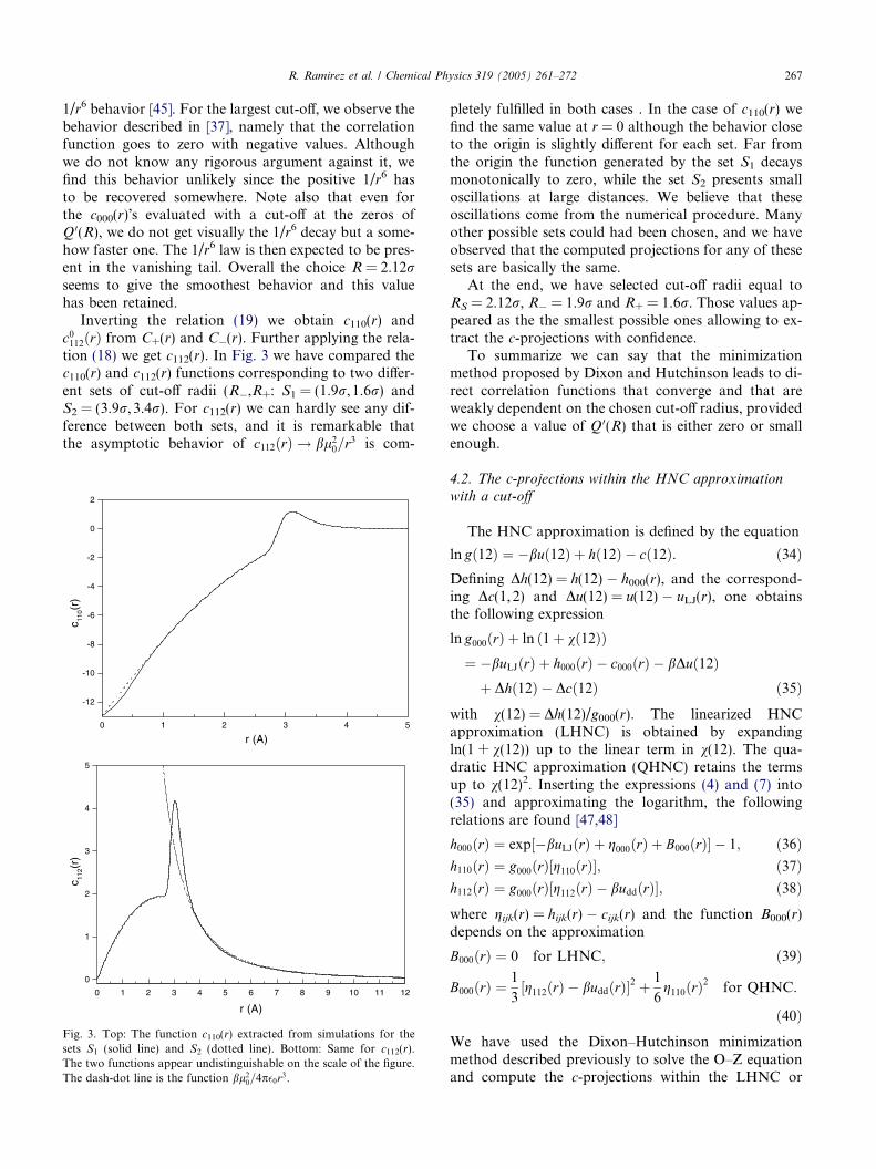
Inverting the relation (19) we obtain c110(r) andc0112ðrÞ from C+(r) and C(r). Further applying the rela-tion (18) we get c112(r). In Fig. 3 we have compared thec110(r) and c112(r) functions corresponding to two differ-ent sets of cut-off radii (R,R+: S1 = (1.9r, 1.6r) andS2 = (3.9r, 3.4r). For c112(r) we can hardly see any dif-ference between both sets, and it is remarkable thatthe asymptotic behavior of c112ðrÞ ! bl2

0=r3 is com-

0 1 2 3 4 5

-12

-10

-8

-6

-4

-2

0

2

c 110(

r)

r (A)

0 1 2 3 4 5 6 7 8 9 10 11 12

0

1

2

3

4

5

c 112(

r)

r (A)

Fig. 3. Top: The function c110(r) extracted from simulations for thesets S1 (solid line) and S2 (dotted line). Bottom: Same for c112(r).The two functions appear undistinguishable on the scale of the figure.The dash-dot line is the function bl2

0=4p0r3.

pletely fulfilled in both cases . In the case of c110(r) wefind the same value at r = 0 although the behavior closeto the origin is slightly different for each set. Far fromthe origin the function generated by the set S1 decaysmonotonically to zero, while the set S2 presents smalloscillations at large distances. We believe that theseoscillations come from the numerical procedure. Manyother possible sets could had been chosen, and we haveobserved that the computed projections for any of thesesets are basically the same.

At the end, we have selected cut-off radii equal toRS = 2.12r, R = 1.9r and R+ = 1.6r. Those values ap-peared as the the smallest possible ones allowing to ex-tract the c-projections with confidence.

To summarize we can say that the minimizationmethod proposed by Dixon and Hutchinson leads to di-rect correlation functions that converge and that areweakly dependent on the chosen cut-off radius, providedwe choose a value of Q 0(R) that is either zero or smallenough.

4.2. The c-projections within the HNC approximationwith a cut-off

The HNC approximation is defined by the equation

ln gð12Þ ¼ buð12Þ þ hð12Þ cð12Þ. ð34ÞDefining Dh(12) = h(12) h000(r), and the correspond-ing Dc(1,2) and Du(12) = u(12) uLJ(r), one obtainsthe following expression

ln g000ðrÞ þ ln 1þ vð12Þð Þ¼ buLJðrÞ þ h000ðrÞ c000ðrÞ bDuð12Þ

þ Dhð12Þ Dcð12Þ ð35Þwith v(12) = Dh(12)/g000(r). The linearized HNCapproximation (LHNC) is obtained by expandingln(1 + v(12)) up to the linear term in v(12). The qua-dratic HNC approximation (QHNC) retains the termsup to v(12)2. Inserting the expressions (4) and (7) into(35) and approximating the logarithm, the followingrelations are found [47,48]

h000ðrÞ ¼ exp½buLJðrÞ þ g000ðrÞ þ B000ðrÞ 1; ð36Þh110ðrÞ ¼ g000ðrÞ½g110ðrÞ; ð37Þh112ðrÞ ¼ g000ðrÞ½g112ðrÞ buddðrÞ; ð38Þwhere gijk(r) = hijk(r) cijk(r) and the function B000(r)depends on the approximation

B000ðrÞ ¼ 0 for LHNC; ð39Þ

B000ðrÞ ¼1

3g112ðrÞ buddðrÞ½ 2 þ 1

6g110ðrÞ

2 for QHNC.

ð40ÞWe have used the Dixon–Hutchinson minimizationmethod described previously to solve the O–Z equationand compute the c-projections within the LHNC or


QHNC theory. For this, we used the same real-spacegrid as in the previous section. Starting from a trial seth000(r), h110(r) and h112(r) we compute the correspondingHS(r), H+(r) and H(r) functions, and with the minimi-zation method we find the CS(r), C+(r) and C(r) func-tions. The c-projections are derived from these functionsand inserted into the right-hand side of Eqs. (36)–(38),together with the current values of the h-projections,in order to calculate a new set of h-projections. The iter-ation continues until the convergence of the functions isachieved.

Note that we have chosen for the functions C(r) cut-off radii located in the same range as for the MD func-tions above, namely 1.5r 6 R 6 2.5r for all the S, + and functions. The reason is that the functions Q 0(r) in theLHNC and QHNC theories present zeros up to muchlarger distances than the ones encountered in MD simu-lations, and the resulting c(r) projections can vary sub-stantially from one zero to another. In fact, we havefound that the larger the cut-off radius R, the smallerare the values found for the functions c(r) at the origin.This result is also commented in [42].

In Fig. 4, the function c000(r) calculated with theLHNC and QHNC approximations is compared withthe one extracted from MD simulations of the Stockma-yer solvent. The function c000(r) is similar in shape butquite different at the origin (cMD

000 ð0Þ ¼ 17.0,cLHNC000 ð0Þ ¼ 18.7 and cQHNC

000 ð0Þ ¼ 15.9). All of thempresent a derivative discontinuity at r r. The LHNCand QHNC functions decay exactly as the imposed 1/r6 potential whereas the MD function is found to decayslightly faster at intermediate ranges.

The same comparison between LHNC/QHNC andMD leads to a better agreement for c110(r) with a verysimilar behavior close to r = 0. As for c112(r), the variouscurves appear visually undistinguishable on a scale sim-ilar to that of Fig. 3.

0 1 2 3 4 5 6

-18

-16

-14

-12

-10

-8

-6

-4

-2

0

2

c 000(

r)

r (A)

Fig. 4. The function c000(r) calculated from: MD simulations (dottedline), LHNC theory (dash line) and QHNC theory (solid line).

5. Application to density functional theory: solvation of

simple solutes

Using as input the MD, LHNC or QHNC direct cor-relation functions, the functional defined in Eqs. (8)–(11) can be minimized for any external field Vext(r,X)to yield the equilibrium density and polarization. Wehave studied the case of a spherical Lennard–Jones par-ticle (with same parameters r, as the solvent) andcharge +e at its center. This solute particle was placedin a cubic box of side 36 A with periodic boundary con-ditions and the functional was minimized on a grid of643 points corresponding to a spacing of 0.5 A. The min-imization was done for n(r) and the mean orientationX(r) = P(r)/l0n(r).

In Fig. 5 the solvent radial density around the sol-vated ion computed by direct MD simulations is com-pared to the ones obtained by DFT minimization withthe set of the c-projections corresponding to MD,LHNC and QHNC. All the three direct correlationfunctions give roughly the same prediction for the den-sity, although the QHNC approximation overestimatesthe density at the first peak and all of them overestimatethe second peak . The profiles do not depend on the cut-off chosen for the direct correlation functions. We havetested a number of c-functions generated from differentcut-off radius, obtaining always very similar results. Thediscrepancies between the ‘‘exact’’ MD simulation andthe minimization results come either from the approxi-mation of the functional itself (the homogeneous refer-ence fluid approximation) or from the fact that higherorder c-projections in the basis of rotational invariantsare not contained in the description.

Fig. 6 displays the average orientation XðrÞ ¼hXðrÞi r at a distance r from the charge. Visually, it

2 4 6 8 10 120

1

2

3

4

5

6

n(r

)

r (A)

Fig. 5. The radial density n(r) calculated from: MD simulations(circles) and DFT minimization with: MD (solid line), LHNC (dotsline), and QHNC (dash line) direct correlation functions.

3 4 5 6 7 8 9 10 11 120.0

0.3

0.6

0.9

Ω(r

)

r (A)

4 5 6 70.0

0.1

0.2

0.3

0.4

0.5

r(A)

Ω(r

)

Fig. 6. The modulus of the average orientation in the radial directionX(r) calculated from: MD simulations (circles) and minimization with:MD (solid line), LHNC (dots line), and QHNC (dash line) directcorrelation functions.


can be observed that the MD-based functional is doingslightly better, especially at and beyond the second peak.However, the two HNC approximations give very rea-sonable results too. In Fig. 7, we have compared theelectrostatic solvation free energy for different valuesof the solute charge. This electrostatic free energy isthe difference between the value of the functionalG[n,P] for a solute of charge q and the same functionalevaluated for q = 0. We have thus subtracted the freeenergy of the solvent in the presence of a neutral Len-nard–Jones particle. The results corresponding to thethree input correlation functions are very close and ingood agreement with the direct MD simulations (errorbars are not given but they do match the DFT values).This proves that the energetics is not very sensitive to

0.0 0.1 0.2 0.3 0.4 0.5 0.6 0.7 0.8 0.9 1.0

-350

-300

-250

-200

-150

-100

-50

0

∆Gel (

kJ /

mo

l)

charge (e)

Fig. 7. Solvation energies X(r) calculated from: MD simulations(circles) and DFT minimization with: MD (solid line), LHNC (dotsline), and QHNC (dash line) direct correlation functions.

slight differences in the c-functions which are injectedin the functional.

At last, in order to assess the performance of ourfunctional approach for a less trivial case, we have con-sidered the solvation of prototypical dipolar molecule,N-methyl-acetamide molecule (NMA), in our molecularsolvent. This molecule constitutes an elementary build-ing block for peptides and proteins, and, as such, itserves as a special model for theoretical calculations.This molecule can be found in two isomeric cis and trans

forms corresponding to the isomerization of a peptidebond. The free energy difference between the two iso-mers has been the determined both experimentally andcomputationally.

The geometrical configuration of the two isomers isdisplayed in Fig. 8. We compare in Figs. 9 and 10 thecorresponding solute-atoms/solvent-atom radial distri-bution functions computed by molecular dynamics tothose obtained by minimization of the solvent densityfunctional in the presence of the molecule. In the lattercase, the radial distribution functions can be identifiedto the mean density at a distance r of a given atomic site.The OPLS Lennard–Jones parameters and partialcharges for NMA were taken from [52]; the CH3 terminiare considered as a single effective site. The MD simula-tions were carried out with one NMA molecule dis-solved in 512 solvent particles for a total time of250 ps. The DFT calculation was performed with abox of grid size of 0.25 A and 1283 grid points. It canbe seen again in the various figures that the DFT ap-proach is doing quite well. The finite grid representationof the functional remains apparent but, overall, the var-ious density peaks are correctly reproduced in both posi-tions and intensities. The fact that our DFT approach isable to capture correctly the solvent structure around amolecule having a complex three-dimensional shape andcharge distribution is quite encouraging. The judicious-ness of the conjecture is here demonstrated for a ‘‘real-istic’’ molecular solute in a dipolar fluid. It certainlyneeds further extensive testing for other complex solutesand/or solvents.

In order to assess the importance of electrostatic ef-fects and of including non-spherical rotational invari-ants in our functional description, i.e., to go beyondthe conventional HNC theory, we have also minimizeda reduced functional in which only the spherical interac-tions were considered (c000(r) and the Lennard–Jonescontributions to the external potential). In Fig. 11, wehave compared the amide H-solvent radial distributionfunction with and without dipolar terms. It can be seenthat the first peak corresponding to a solvent moleculealmost permanently attached to the H positive chargedisappears completely when the dipolar interactionsare turned off. As for the long range solvent structure,it remains globally the same and seems dominated bysolvent packing effects. We have also computed the

Fig. 8. Geometrical configuration of cis (left) and trans (right) N-methylacetamide (formula: CH3-NH-CO-CH3).

Fig. 9. Atom-solvent radial distribution functions for cis-N-methylacetamide in the Stockmayer solvent: (a) oxygen, (b) amide hydrogen, (c)backbone carbon (bottom curves) and nitrogen (top curves, upshifted by 1), (d) C-terminal methyl (bottom) and N-terminal methyl (top, upshiftedby 1.5). The solid and dashed lines correspond to the DFT and MD results, respectively.

Fig. 10. Same as Fig. 9 for trans-N-methylacetamide.


Fig. 11. Amide H-solvent radial distribution functions for trans-N-methylacetamide with (solid line) and without (dashed line) inclusionof the dipolar interactions in the functional.


solvation free-energy difference between the trans and cis

form. This requires only two DFT minimizations, onefor each isomeric form illustrated in Figs. 9 and 10,whereas an equivalent calculation using moleculardynamics or Monte-Carlo simulations requires a numer-ically costly thermodynamic integration path with a tor-sional angle U varying progressively from the cis form(0) to the trans form (180) [52]. We find that the cis–trans free energy difference turns from positive(+1.7 kJ/mol) to negative (2.7 kJ/mol) when the dipo-lar terms are turned off. This and the structural effectsdescribed above illustrate the importance of includingthe right number of spherical invariants into the func-tional description.

Beyond numbers, the calculations presented for a sol-vated NMA molecule prove that (i) minimizing a ratherdetailed microscopic functional around a complex shapesolute is numerically feasible at a rather modest cost(compared to a full MD or MC simulation), and (ii)the great advantage of the functional minimization ap-proach is that the overall free energy difference doesnot require any thermodynamic integration scheme, asin explicit simulations, and it can be obtained with onlyTWO calculations, one for the starting configurationand one for the final one. Furthermore, both the averagesolvation structure and the absolute solvation free en-ergy are obtained with a single minimization. Account-ing for the flexibility of the solute would be possibleby extending the ‘‘on-the-fly’’ minimization procedureof [5].

6. Conclusions

The position and angle-dependent direct correlationfunction is the key quantity entering in the density func-tional theory description of inhomogeneous molecularfluids submitted to external potentials. In the homoge-

neous reference fluid approximation, this function isapproximated by that of the homogeneous fluid of equalchemical potential, thus in the absence of any externalperturbation. We have shown in this paper that, at leastfor dipolar fluids, the homogeneous direct correlationfunction can be inferred to a good approximation byfirst computing ‘‘exact’’ position and angular two-bodycorrelations using MD or MC simulation methods,and then inverting the Ornstein–Zernike equation. Toour knowledge, this is the first time that this approachproves to be possible and valuable for a polar fluid withlong range interactions. The ‘‘exact’’, MD direct correla-tion functions have been compared to those which canbe obtained from integral equation theories such asLHNC and QHNC. We found that those theories doprovide reasonable c-functions (and more so for QHNCthan for LHNC, as expected). As a matter of principlehowever, and for further developments with more com-plicated interactions, it is important to know that directcorrelation functions can be considered as (as much aspossible) ‘‘exact’’ quantities which can be safely ex-tracted from simulations. The MD and integral equationc-functions were then injected into the definition of asolvent free-energy density functional, and the validityof the functional approach was tested on the solvationproperties of simple spherical solutes in the dipolar sol-vent. When compared to molecular dynamics, the re-sults of the functional minimization turn out to bevery encouraging and the validity of the method wasalso confirmed recently for molecular solutes with com-plex shapes [30]. We are planning to continue our ap-proach for more realistic solvent models reproducingthe properties of liquid water. This can be done by eitheradjusting our generic dipolar functional to the experi-mental structure factor and non-local dielectric proper-ties of water [27,28] or by generalizing it to accountfor quadrupolar or higher-order multipolar interactions[36]. We believe that our density functional theory ap-proach provides a flexible, improvable, and universaltool to estimate the absolute solvation free energy ofcomplex molecular entities and, by difference, the reac-tion free energy of any complex charge transfer reactionin solution.

References

[1] R. Marcus, J. Chem. Phys. 24 (1956) 956.[2] V.G. Levich, R.R. Dogonadze, Dokl. Acad. Nauk. SSSR 124

(1959) 123.[3] A.M. Kuznetsov, Charge Transfer in Physics, Chemistry, and

Biology, Gordon and Breach, Reading, 1995.[4] A.M. Kuznetsov, J. Ulstrup, Electron Transfer in Chemistry and

Biology: An Introduction to the Theory, Wiley, Chichester, 1999.[5] M. Marchi, D. Borgis, N. Levy, P. Ballone, J. Chem. Phys. 114

(2001) 4377.[6] A. Warshel, J. Phys. Chem. 86 (1982) 2218.[7] J.K. Hwang, A. Warshel, J. Am. Chem. Soc. 109 (1987) 715.


[8] M. Marchi, J. Gehlen, D. Chandler, M. Newton, J. Am. Chem.Soc. 115 (1993) 4178.

[9] H. Azzouz, D. Borgis, J. Chem. Phys. 98 (1993) 7361.[10] T. Simonson, G. Archantis, M. Karplus, Acc. Chem. Res. 35

(2002) 430.[11] T. Simonson, Proc. Natl. Acad. Sci. USA 99 (2002) 6544.[12] P. Kollman, Chem. Rev. 93 (1993) 2395.[13] A.A. Kornyshev, in: R.R. Dogonadze, E. Kalman, A.A. Korni-

shev, J. Ulstrup (Eds.), The Chemical Physics of Solvation, Vol.A, Elsevier, Amsterdam, 1985, p. 77.

[14] M.A. Vorotyntsev, A.A. Kornyshev, Electrostatics of a Mediumwith the Spatial Dispersion, Nauka, Moscow, 1993.

[15] A.A. Kornyshev, G. Sutmann, J. Chem. Phys. 104 (1996) 1564.[16] A.A. Kornyshev, G. Sutmann, Electrochim. Acta 42 (1997) 2801.[17] F.O. Raineri, H.L. Friedman, Adv. Chem. Phys. 107 (1999) 81.[18] D. Matyushov, J. Chem. Phys. 120 (2004) 7532.[19] B. Bagchi, A. Chandra, Adv. Chem. Phys. 80 (1991) 1.[20] L.E. Fried, S. Mukamel, J. Chem. Phys. 93 (1990) 932.[21] A. Chandra, D. Wei, G.N. Patey, J. Chem. Phys. 99 (1993) 2068.[22] A. Chandra, D. Wei, G.N. Patey, J. Chem. Phys. 99 (1993) 4926.[23] F.O. Raineri, H.L. Friedman, J. Chem. Phys. 98 (1993) 8910.[24] F.O. Raineri, H. Resat, B.C. Perng, F. Hirata, H.L. Friedman, J.

Chem. Phys. 100 (1994) 1477.[25] T. Fonseca, B. Ladanyi, J. Chem. Phys. 93 (1990) 8148.[26] M.S. Skaf, T. Fonseca, B. Ladanyi, J. Chem. Phys. 98 (1993) 8929.[27] P. Bopp, A.A. Kornyshev, G. Suttmann, Phys. Rev. Lett. 76

(1996) 1280.[28] P. Bopp, A.A. Kornyshev, G. Suttmann, J. Chem. Phys. 109

(1996) 1939.[29] R. Ramirez, R. Gebauer, M. Mareschal, D. Borgis, Phys. Rev. E

66 (2002) 031206.

[30] R. Ramirez, D. Borgis, J. Phys. Chem. B 109 (2005) 6754.[31] X. Song, D. Chandler, J. Chem. Phys. 108 (1998) 2594.[32] X. Song, D. Chandler, R.A. Marcus, J. Phys. Chem. 100 (1996)

11954.[33] D. Chandler, J.D. McCoy, S.J. Singer, J. Chem. Phys. 85 (1986)

5971.[34] D. Chandler, J.D. McCoy, S.J. Singer, J. Chem. Phys. 85 (1986)

5977.[35] T. Biben, J.P. Hansen, Y. Rosenfeld, Phys. Rev. E 57 (1998)

R37227.[36] S.L. Carnie, G.N. Patey, Mol. Phys. 47 (1982) 1129.[37] M. Dixon, P. Hutchinson, Mol. Phys. 33 (1977) 1663.[38] E.L. Pollock, B.J. Alder, Physica A 102 (1980) 1.[39] R.J. Baxter, Austr. J. Phys. 21 (1968) 563.[40] L. Blum, J. Chem. Phys. 57 (1972) 1862.[41] L. Blum, A.J. Torruella, J. Chem. Phys. 56 (1972) 303.[42] L.M. Sese, R. Ledesma, J. Chem. Phys. 106 (1997) 1134.[43] M.P. Allen, C.P. Mason, E. de Miguel, J. Stelzer, Phys. Rev. E 52

(1995) R25.[44] G. Stell, G.N. Patey, J.S. Hoye, Adv. Chem. Phys. 48 (1981)

183.[45] G. Stell, Physica 29 (1963) 517.[46] W. Smith, CCP5 Inf. Quart. 4 (1982) 13.[47] M.S. Wertheim, J. Chem. Phys. 55 (1971) 4291.[48] G.N. Patey, D. Levesque, J.J. Weis, Mol. Phys. 38 (1979) 219.[49] J.P. Hansen, J.R. McDonald, Theory of Simple Liquids, Aca-

demic Press, London, 1989.[50] M.P. Allen, D.J. Tildesley, Computer Simulations of Liquids,

Oxford University Press, New York, 1987.[51] L.Y. Lee, P.H. Fries, G.N. Patey, Mol. Phys. 55 (1985) 751.[52] W. Jorgensen, J. Gao, J. Am. Chem. Soc. 110 (1988) 4212.

direct correlation functions and the density functional theory of polar solvents

Documents