dimitris georgarakos,michael haliassos, and giacomo pasini · * we would like to thank rob alessie,...

Center for Financial Studies Goethe-Universität Frankfurt House of Finance

Grüneburgplatz 1 60323 Frankfurt Deutschland

Telefon: +49 (0)69 798-30050 Fax: +49 (0)69 798-30077 http://www.ifk-cfs.de E-Mail: [email protected]

No. 2012/05

Household Debt and Social Interactions

Dimitris Georgarakos,Michael Haliassos, and Giacomo Pasini

CFS WO R K I N G PA P E R

Center for Financial Studies Goethe-Universität House of Finance

Grüneburgplatz 1 60323 Frankfurt am Main Deutschland

Telefon: +49 (0)69 798-30050 Fax: +49 (0)69 798-30077 http://www.ifk-cfs.de E-Mail: [email protected]

Center for Financial Studies

The Center for Financial Studies is a nonprofit research organization, supported by an association of more than 120 banks, insurance companies, industrial corporations and public institutions. Established in 1968 and closely affiliated with the University of Frankfurt, it provides a strong link between the financial community and academia.

The CFS Working Paper Series presents the result of scientific research on selected topics in the field of money, banking and finance. The authors were either participants in the Center´s Research Fellow Program or members of one of the Center´s Research Projects.

If you would like to know more about the Center for Financial Studies, please let us know of your interest.

Prof. Michalis Haliassos, Ph.D. Prof. Dr. Jan Pieter Krahnen Prof. Dr. Uwe Walz

* We would like to thank Rob Alessie, Bas Donkers, Yannis Ioannides, Mauro Mastrogiacomo, Luigi Pistaferri, Dorothea Schäfer, Kostas Tatsiramos, and seminar participants at the NETSPAR International Pension Workshop, Amsterdam; at the Behavioral Finance Conference, DIW, Berlin; at the 10th Conference on Economic Theory and Econometrics (CRETE), Milos, Greece; at the Association of Southern European Economic Theory (ASSET) conference in Evora, Portugal; at the GSEFM conference in Mainz, Germany; at the Universities of Bath and of Southampton; and at the research department of Deutsche Bundesbank. Haliassos acknowledges research funding from the German Research Foundation (DFG).

1 Goethe University Frankfurt and CFS 2 Corresponding author: Goethe University Frankfurt, CFS and CEPR, E-mail: [email protected] 3 University of Venice “Ca’ Foscari” and NETSPAR

CFS Working Paper No. 2012/05

Household Debt and Social Interactions*

Dimitris Georgarakos1,Michael Haliassos2, and Giacomo Pasini3

March 1, 2012

Abstract Debt-induced crises, including the subprime, are usually attributed exclusively to supply-side factors. We examine the role of social influences on debt culture, emanating from perceived average income of peers. Utilizing unique information from a household survey representative of the Dutch population, that circumvents the issue of defining the social circle, we consider collateralized, consumer, and informal loans. We find robust social effects on borrowing, especially among those who consider themselves poorer than their peers; and on indebtedness, suggesting a link to financial distress. We employ a number of approaches to rule out spurious associations and to handle correlated effects. JEL Classifications: G11, E21 Keywords: Household Finance, Household Debt, Social Interactions, Mortgages,

Consumer Credit, Informal Loans

2

1. Introduction

The recent financial crisis has demonstrated the potential of sizeable household

groups to borrow at levels that expose them to subsequent difficulties in servicing debts and

to a non-trivial risk of default. For example, many US households had exposed themselves to

excessive mortgage debt prior to the subprime crisis, and some ended up with negative equity

following the reversal of historical house price trends. Existing literature and public

discussion have paid attention, almost exclusively, to supply-side factors that may have

contributed to this tendency, such as lax standards of the banking sector, the transfer of risks,

and the resulting lack of discipline in applying sound banking standards.1

Much less attention has been devoted to understanding demand-side factors that

contribute to the spread of debt culture, especially among households who perceive

themselves as having fewer resources than their peers on average. An important example of

such factors, albeit specific to the subprime crisis, is the subjective belief of borrowers that

US house prices could not fall, based on the long historical experience of price increases.

2

The importance of relative standing in the social circle has long been recognized in

the economics and finance literature, but for issues other than debt. Models with

Our paper focuses on another factor, which could apply to all types of debt and has been

explored only in other contexts: comparison with peers. If expectations or perceptions of

relative standing are important for debt behavior, then regulation and monitoring of financial

institutions may need to be combined with measures for households, such as financial

education, proper advice, and appropriate default options, in order to contain the spread of

debt culture and the risks for future debt-induced financial crises.

1 See for example, Mian and Sufi (2009) who show that a shift in credit supply was a key factor in the expansion of subprime mortgages in the US; and Demyanyk and Van Hemert (2012) who find that the quality of such loans deteriorated for six consecutive years prior to the crisis. Using recently available data, Christelis, Georgarakos and Haliassos (forthcoming) show that shortly prior to the recent crisis, outstanding mortgages were substantially larger among older US households than their European counterparts with similar resources and characteristics. 2 See, for example, the contributions by Case (2012), Shiller (2012), and Smith (2012).

3

interdependent preferences have been applied to consumption (Duesenberry, 1949; Abel,

1990; Gali, 1994, Kapteyn et al., 2011); asset pricing (Campbell and Cochrane, 1999);

investing in assets (Duflo and Saez, 2002; Hong, Kubik and Stein, 2004; Kaustia and

Knüpfer, forthcoming); supply of labor (Neumark and Postlewaite, 1998); work effort (Cohn

et al., 2011); and short-run stabilization policy (Ljungqvist and Uhlig, 2000). To the best of

our knowledge, this is the first paper that investigates the role of social interactions and

comparison effects for borrowing behavior.

Our paper exploits unique features of a population-wide survey to uncover a

statistically and economically significant influence of perceived relative standing on

household debt behavior. Specifically, we employ data from the population-wide Dutch

National Bank (DNB) Survey, and consider three different types of debt, namely

collateralized loans, consumer non-collateralized loans, as well as informal loans from the

social circle.

We find that the higher the average income in the social circle, as perceived by a

household, the more this household tends to borrow, controlling for own demographics,

resources, and other factors that typically determine borrowing needs. Estimated effects are

sizeable both for collateralized and consumer debt. A 1,000 euro increase in the monthly

household income of the peers is estimated to raise by 10 percent (7 percent) the

unconditional likelihood of having collateralized (uncollateralized consumer) loans,

respectively. Moreover, the influence of peer income on debt behavior is stronger among

those who perceive their income to be below average for their social circle. Interestingly,

higher perceived income of peers is associated not only with more borrowing but also with

measures of household financial debt burden. As we discuss in detail later, we undertake a

number of steps to rule out uninteresting alternative explanations of the relationship and to

address the potential for a spurious correlation between the two due to similarity in

4

unobserved characteristics of the respondent or its environment with those of the peers. These

latter steps include estimation of different instrumental variable regression models and

application of placebo tests.

Uncovering effects of social interactions on borrowing behavior poses some special

challenges, not necessarily present in other domains. First, information about characteristics

of the social circle is not typically available in most wealth surveys, as they are subject to a

high degree of anonymization, intended to prevent identity disclosure. Anonymization

involves omitting or heavily restricting information on location in regions, let alone

neighborhoods. Faced with this challenge, research on social interactions on the asset side

attempts to identify peer effects by constructing hypothesized social circles based on sorting

assumptions (e.g., age and education); or by focusing on specific financial products and

social groups where interactions are visible (e.g., retirement plans in particular

establishments); or by considering the frequency of meetings, where presumably assets (but

typically not debts) are discussed or displayed.

The DNB Survey contains unique information that allows us to overcome this

limitation. The survey asks respondents to describe key features of their social circle (e.g.,

age, education, occupation) and importantly the perceived average income of their peers.

Moreover, the data offer information on the entire range of household debts, formal and

informal, collateralized and unsecured, as well as on financial and real assets, as opposed to a

single financial product. Finally, the survey is representative of the entire Dutch population,

as opposed to a particular group.

An additional challenge is that, while households may derive some pleasure from

revealing their wages, consumption or asset levels to their social circle (or may be unable to

hide them), they tend to be quite averse to revealing debt levels, protected also by bank

confidentiality. Thus, the important channel through which peer effects are likely to operate

5

is not direct observation and emulation of borrowing behavior among peers, but rather

observation of some key determinant of such behavior (e.g., a measure of resources or ability

to spend). In this context, we investigate the link between average peer income, as perceived

by respondents, and the respondents’ own borrowing behavior.

Our paper relates closely to three different strands of literature: effects of social

interactions on asset choices; the relative income hypothesis and external habits; and finally,

the literature on ‘envy versus ambition’.

Duflo and Saez (2002) study library staff members in different libraries of a big

American university and show that individual participation in retirement investment plans is

influenced by participation choices of colleagues. Such endogenous social effects could come

from learning about assets or from discovering relevant social norms, but it is difficult to

distinguish between these two. Hong, Kubik and Stein (2004) focus instead on sociability,

and show that the more sociable in terms of certain self-reported metrics (i.e., frequent

communication with neighbors and church-going) are more likely to own stocks.3

The importance of peer income was stressed in the (cross-sectional) formulation of

Duesenberry’s (1949) relative income hypothesis, built on insights in Veblen (1899) and

Smith (1759). According to this hypothesis, households with incomes below average in their

social circle will tend to consume a larger share of their income to keep up with peers. In

modern analysis of consumption and asset pricing, a fine distinction was made between

dependence on contemporaneous average peer consumption (‘keeping up with the Joneses’)

and lagged average consumption (‘catching up with the Joneses’).

4

3 Brown et al. (2008) identify a causal influence of sociability on stockholding by instrumenting the average stock ownership of an individual’s community with past average ownership of the US states in which the individual’s non-native neighbors were born. Georgarakos and Pasini (2011) document effects of sociability on stockholding in Europe.

Recently, Kapteyn et al.

(2011) have examined the effects on consumption of winning a Dutch postal code lottery,

4 More recently, Roussanov (2010) built a model of status, where utility is a function of relative wealth and households are characterized by a desire to ‘get ahead of the Joneses’, focusing on private business ownership.

6

both among lottery winners and among their neighbors. Using specially collected survey data

on expenditures and different assumptions on the social circle, the authors find that

exogenous variations in income due to winning the lottery tend to influence durables

purchases by winners but also the probability that neighbors will buy a new car. Their survey

did not collect any information on debts or on perceptions of participants regarding their

peers.

It should be stressed that the research question of social influences on debt is distinct

from the one relating to consumption: even if concern with relative standing leads to greater

consumption, it may not necessarily lead to a greater tendency to borrow. For instance, if

households increase labor supply, relative income concerns can increase both consumption

and saving. Indeed, Neumark and Postlewaite (1998) found that married women in the US are

16 to 25 percent more likely to work outside the home if their sisters’ husbands earn more

than their own husbands. Even a positive labor supply response, however, could imply either

more or less saving/ borrowing.5

A third strand of literature has studied the link between relative income and self-

reported happiness or general well-being. Relative income could measure relative

deprivation, or create anticipatory feelings because lower-income households use it as a

signal of the (higher) income they, too, can earn in the future. A number of studies have

found that individual subjective well-being is negatively influenced by others’ income

6

5 Most existing theoretical models, based on an infinite-horizon representative agent, imply greater consumption, less leisure, and greater accumulation of assets, in order to keep up with the Joneses also in the future (Liu and Turnovsky, 2005). By contrast, Alvarez-Cuadrado and Van Long (2008) obtain less leisure but also lower saving when they consider overlapping generations in an infinite-horizon economy.

, while

utility-enhancing ‘anticipatory feelings’ (Caplin and Leahy, 2001) have been stressed by

Hirschmann and Rothschild (1973), who dubbed them ‘Tunnel Effect’. The idea is that, if

6 For example, Clark and Oswald (1996) show that a worker’s job satisfaction is negatively influenced by the income earned by other individuals in her reference group. Ferrer-i-Carbonell (2005) using German panel data finds that individuals tend to be better-off the larger their income is in comparison with the income of their acquaintances.

7

you are caught in a traffic jam in a tunnel and you see the other lane moving, you anticipate

that you will also move soon.7

The rest of the paper is organized as follows. Section 2 describes the unique features

of our data set. Section 3 discusses possible channels through which peers might influence

borrowing behavior, and the econometric approach to address a number of challenges.

Section 4 presents the main results on the relationship between perceived income of peers and

own debt behavior, including endogeneity tests and IV estimates. Section 5 presents

additional robustness checks and placebo tests. Section 6 presents evidence of asymmetric

effects on borrowing across households poorer and richer than the peer average and inspects

likely channels through which peer income operates. Section 7 concludes.

The effect on borrowing may, in the end, be positive, either

when households are disappointed by their current relative income or when they expect a

positive income growth rate.

2. The Data

The DNB Survey is a unique data set that allows the study of both psychological and

economic aspects of financial behavior. The survey was launched in 1993 and includes

information on work, pensions, housing, mortgages, income, assets, consumer loans, health,

economic and psychological concepts, and personal characteristics. The initial survey

consists of around 2,790 Dutch households that are oversampled from the top-10% of the

income distribution and (with the use of survey weights) is representative of the Dutch-

speaking population. Households have been re-interviewed each following year, but given the

length of the panel, attrition was non-negligible. In order to keep the cross section sample

representative, new households have been added each year, with a major refreshing in 2001,

7 Senik (2004) finds empirical support for the ‘Tunnel Effect’ using survey data from Russia, while Senik (2008) documents a negative comparison income effect in many ‘old’ European countries, and a positive one (i.e., consistent with a ‘Tunnel Effect’) in East European countries and the US, mainly linked to the degree of income mobility.

8

resulting in a sample of 1,861 households. In view of this significant refreshing, we pool data

only from waves between 2001 until 2008, which cover a period of relatively stable

employment rates and increasing housing prices8

The survey includes an extensive questionnaire covering income, real and financial

wealth holdings. Debt related questions allow us to distinguish between collateralized and

non-collateralized debt as well as loans from friends and relatives. In what follows, we will

mainly focus on consumer debt and collateralized debt, but we also present results on

informal loans (from friends and relatives).

, and we employ survey weights to account

for the over-representation of the wealthy. After excluding households with incomplete

questionnaires or missing information on the characteristics of their social circle, the sample

used in the baseline estimations consists of roughly 4,500 households.

Table 1 provides summary statistics on the prevalence and the amounts outstanding

among debt holders by survey year and by loan type. Reported statistics suggest relatively

stable prevalence of all three types of loans over the years we examine. Collateralized debts

account for most of household borrowing. They are held by roughly 40% of households and

the median conditional outstanding amount is about 98,000 euro. One out of five Dutch

households has consumer loans with a median outstanding amount of roughly 4,000 euro. On

the other hand, 4% report loans from friends and relatives, while almost 28% report that they

can borrow from friends in the future.

A unique feature of the Dutch survey, most relevant for our purposes in this paper, is

that individuals are asked to report explicitly a number of characteristics of the people with

whom they “associate frequently, such as friends, neighbors, acquaintances, or maybe people

at work”. In particular, respondents report their perception of the average annual total net

household income among people in their social circle. Answers are recorded in one out of 8 Unemployment rates in the Netherlands reach a minimum of 3% in 2008, while they increase to 3.7% and 4.5% in 2009 and 2010, respectively. National housing prices increase on average by roughly 2% each year up to 2008, while they decline by 2.8% in 2009 and by 3.4% in 2010.

9

eleven income brackets (details are provided in the appendix). Respondents also report the

age category most members of their social circle belong to, the average household size, the

average education, the most prevalent kind of employment in their social circle, and the

average hours of work per week among peers, distinguished by gender.

Furthermore, the survey asks direct questions about the respondent’s interactions with

peers through financial information exchange or through informal borrowing; perceptions of

the spending ability of the social circle; and expectations regarding future own income. This

information is used below to shed light on the process through which social interactions

influence borrowing behavior.

3. Effects of the Social Circle on Debt Behavior

3.1 Possible Channels

Asset market participation and holdings of peers may influence any member of the

peer group via direct observation of financial behavior, information sharing, and

dissemination of social norms. Peer effects in borrowing behavior, however, are much less

likely to emanate from direct observation of the loans of peers or even from discussions with

them regarding their indebtedness. Unlike assets, loans are not directly observable to third

parties and can only become known to them if the borrowers decide to reveal them.

Borrowers, on the other hand, are less likely to want to discuss their loans, because of

embarrassment or shame, than to exhibit their assets.9

Still, financial advice and consultation with members of the social circle may inform

households about the process of getting formal or informal loans, and/or about the social

norms regarding borrowing; and may even deliver informal loans from the social circle. Our

9 Such considerations have been shown to be important even in countries with underdeveloped credit markets, where informal borrowing is quite widespread. For example, Collins, et al. (2009), using data from Bangladesh, India, and South Africa, find that many indebted households feel ashamed asking relatives for additional credit or they do not wish to reveal their financial situation to close acquaintances.

10

data allow us to identify households that consult with their family, friends, and acquaintances

regarding financial decisions and to take into account explicitly this possible channel of

effects.

Households that do not consult with their social circle regarding financial matters may

still be influenced by observable behavior of that circle in their decision on whether to take

out a loan and how much to borrow. Through social interaction, households form a

perception of the average disposable income of their acquaintances. This could come from a

variety of sources, ranging from direct knowledge of pay scales for acquaintances at work to

open discussions with friends and family, but also to inference of income levels from

observed spending or asset accumulation patterns.10

It is conceivable that perceptions of higher peer income contribute positively to

borrowing through at least three channels: trying to emulate the spending or living standards

of acquaintances (a comparison effect); inferring that more can be borrowed directly from

them in the future; and inferring that future own income is likely to move in the same

direction as has current income of the social circle (an expectations or ‘Tunnel’ effect). Our

survey allows us to take into account the second channel, by asking households directly

whether they are in a position to borrow a significant amount of money from their friends and

relatives; and the third, by asking them to state their expectations about future own income.

As discussed, a key feature of our dataset

is that it asks respondents directly about the perceived average income of their acquaintances

allowing us to assess its influence on own borrowing behavior.

With reference to the first channel, spending behavior or visible accumulation of

assets (such as housing) by members of the social circle may well induce a household to

borrow in order to match it (or exceed it). Our data allow us to observe perceptions regarding

spending ability of peers and to incorporate them in the econometric analysis. Although

10 Indeed, imputation of incomes on the basis of spending items or asset accumulation is sometimes used by tax authorities to fight tax evasion in countries in which such phenomena are widespread.

11

perceptions regarding housing or living standards of peers are not directly available, we

examine their relevance by imputing them based on data reported by households likely to be

considered by the respondents as peers or as sharing key characteristics with them.

3.2 Econometric Specification

In the benchmark specification, we examine whether the tendency of households to

borrow and the size of loans conditional on borrowing are influenced by the average income

that they perceive their peer group to have. Specifically, respondents are asked the following

question: “If you think of your circle of acquaintances, how much do you think is the average

total net income per year of those households?” The possible answers come in brackets. In

our reported results, we use the mid points of these bands, adjusted for inflation, while in the

appendix we provide details on a number of robustness checks that employ different

specifications of this variable.11

Existing literature on social interactions in consumption or asset holdings has focused

on uncovering what Manski (1993) termed ‘endogenous social effects’, namely direct effects

of observing the behavior of others, such as consumption or asset holdings, on own

behavior.

12

Given that debts are typically not observable by members of the social circle (for

various reasons, discussed above), our primary focus is on uncovering ‘exogenous or

contextual effects’. These are influences on debt behavior that emanate from observing (or

forming perceptions) regarding not debts, but key characteristics of peers relevant for debt

Econometric modeling in this setup has to address the ‘reflection problem’ that

naturally arises when the behavior of households in a group is expressed as a function of the

average behavior of the group that includes them.

11 We have experimented with dummy variables for income bands, and with a flag dummy variable for those answering ‘don’t know’, but results are insensitive to these variations. 12 See Durlauf and Ioannides (2010) for a thorough review of methodological issues in social interaction models.

12

behavior, such as peers’ incomes. In this setup the two major challenges are: (i) to rule out

spurious links between peer income and own borrowing behavior that have little to do with a

comparison effect; and (ii) to rule out correlated effects, i.e. an association between own

borrowing and peer income, arising from similarity in unobserved characteristics of the

respondent or the respondent’s environment with those of peers.

In our regressions, we control separately for non linear effects of household resources

in the form of net income, net financial wealth, and net real wealth as well as for net income

of the peers.13

A standard but uninteresting source of an effect of higher perceived income of peers

on own borrowing could be related to an adverse idiosyncratic shock: controlling for own

income, the higher the perceived average income of peers, the greater the chance that the

household has experienced a bad idiosyncratic shock in this period. In such a case, standard

models would prescribe more borrowing to smooth an adverse transitory shock. We control

for this possibility by including in the regression self-reported health, labor market status

dummies, and especially answers to a direct question on whether last year’s income was

‘unusually low’.

In addition, we take into account age (through a second order polynomial),

gender, and educational attainment of the financial respondent as well as marital status and

number of children.

Another possibility is that the respondent’s perception of higher income in the social

circle partly reflects a macro or a regional shock: perceptions improve simply because the

macro-economy performs better or because the region in which most of the social circle is

located does so. We take into account these two channels in a flexible way by including both

year and region fixed effects in all our specifications. 13 We allow for non linear effects of household net income, financial and real wealth, and net income of peers (which all have skewed distributions) by means of the inverse hyperbolic sine (IHS) transformation (i.e., log(x+(x2+1)1/2). The advantage of this, near-logarithmic transformation, is that it is defined for zero and negative values (see also Pence, 2006). Our results are robust to alternative specifications of the aforementioned covariates (e.g., dummies denoting quartiles).

13

The more involved potential channel whereby a positive association between peer

income and borrowing could be generated is the one associated with correlated effects: there

may be unobserved factors that influence both the desire to borrow and the desire to associate

with high-income peers and acquaintances. In the case of informal loans, the link could be

very direct: respondents would be more likely to associate with high-income peers and

relatives in order to borrow from them. In the case of formal loans, the link could be subtler.

For any given need to borrow, higher income friends would be able to provide more informal

loans, reducing the need for formal ones. However, it may also be that unobserved factors

make respondents more likely to borrow using any type of loan, and at the same time

encourage them to associate with peers that are viewed as wealthy and in a position to

provide informal loans. In this case, a spurious positive relationship between peer incomes

and all types of loans might be generated.

One approach to address such problems of correlated effects is instrumental variable

estimation. Instruments should be correlated with the covariate of interest (i.e., perceived

average income of the social circle), and their effects on borrowing should run through peer

income but not through other unobserved factors.

We use two independent sets of instruments that hinge on different identification

assumptions. First, we exploit variation in local labor market conditions and the asymmetric

effects that these can have for the incomes of households with different educational

background. That is, a given difference in educational attainment between the respondent and

her peers can imply a bigger difference in incomes in regions with better conditions for the

highly educated workers. Specifically, we interact regional employment rates in high-tech

sectors with the difference in educational attainment between each respondent and her peers,

while we control for the respondent’s own educational attainment and occupation status, as

14

well as for region fixed effects.14

The second IV strategy follows the recent approach in network literature that exploits

variation in characteristics of members of the social circle, not immediately linked to the

decision maker (De Giorgi, Frederiksen and Pistaferri, 2011). In our data, members of a

couple are asked separately to report the characteristics of their social circles, while we can

distinguish in addition the person who ultimately makes the financial decisions. Thus, we use

as an instrument for the financial decision maker’s perceptions of his or her income of peers

the characteristics of the partner’s social circle, as reported by that partner. The idea is that

the partner forms an estimate of average income in the social circle based on the

characteristics of his/her own acquaintances (age and education), and this in turn influences

the perception of the financial decision maker regarding average income in the decision

maker’s social circle. Such influence could be exerted either because the partner provides a

fresh perspective and more information to the financial decision maker or because the partner

exerts pressure and manages to alter the perceptions of the financial decision maker, even in

ways that are not objectively accurate.

The identification assumption is that the educational gap

between the respondent and her peers will raise the respondent’s perception of her peers’

average income, and more so when the regional employment share in high technology

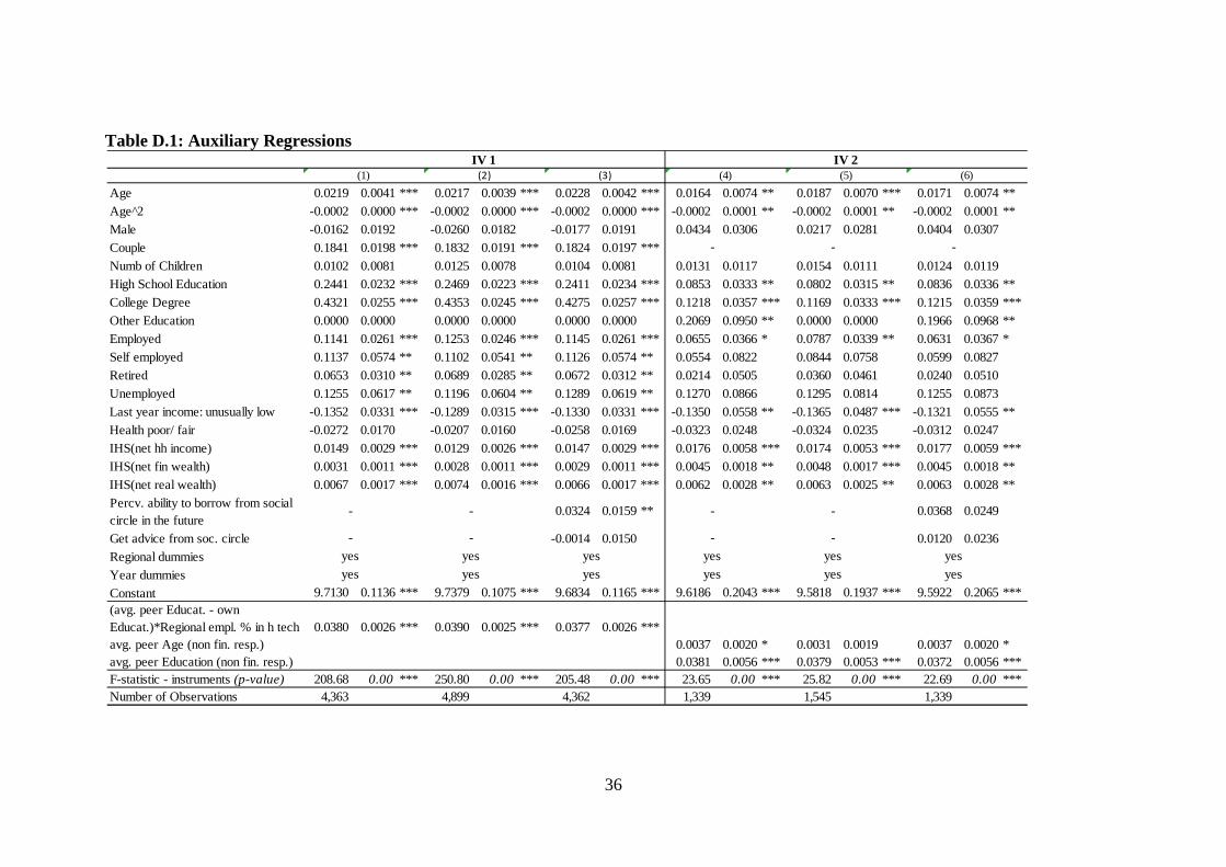
occupations, for which education matters a lot, is larger. Indeed results from the auxiliary

regressions (presented in the Appendix, Table D.1, cols. 1, 2, 3) suggest a strong positive

association between our instrument and the perceived income of the peers.

14 High tech-sectors refer to both high-tech manufacturing industries (manufacture of basic pharmaceutical products and pharmaceutical preparations computer, electronic and optical products) and high-tech knowledge-intensive services (motion picture, video and television programs production, sound recording and music publishing activities; programming and broadcasting activities; telecommunications; computer programming; consultancy and related activities; information service activities; scientific research and development). We calculate employment rates in high-tech sectors across all Dutch provinces, namely: Groningen, Friesland, Drenthe, Overijssel, Flevoland, Gelderland, Utrecht, Noord-Holland, Zuid-Holland, Zeeland, Noord-Brabant, and Limburg.

15

In order to employ this instrument, we have to restrict the sample to couples. We take

a cautious stance by considering only households for which the characteristics of peers

reported differ among the financial decision maker and the partner. This may be due to small

overlap between the social circles of the two partners, or to differences in perceptions of

peers between them. Results from auxiliary regressions are presented in the Appendix (Table

D.1, cols. 4, 5, 6). Given that we utilize two instruments (age and education) for one

potentially endogenous covariate, we can assess their validity using a Sargan-Hansen test for

over-identifying restrictions. As we show in the next section we fail to reject the null that the

employed instruments are valid in all specifications used to model collateralized and

consumer loans.

4. Results on the Role of Peer Income for Borrowing Behavior

We estimate a series of probit and tobit models, modeling the likelihood of having

loans and the (log) amount of loans outstanding, respectively. Standard errors have been

adjusted for heteroskedasticity, allowing for clustering at the household level. To gain

understanding of the economic significance of our findings, we report average marginal

effects for the probit models; and average marginal effects conditional on having the loan

type under examination for the tobit models. We apply the two sets of instruments described

above to all three different types of loans we consider: informal loans, collateralized formal

loans, and consumer (uncollateralized) formal loans.

Table 2 (col. 1) presents average marginal effects from a probit regression modeling

the probability that the respondent thinks that he/she can borrow from friends or relatives in

the future, if needed. The estimated marginal effect of the perceived average income of the

social circle is positive and significant at 1%. It implies that an assumed increase of the

(perceived) annual household income of peers by 12,000 euro (i.e., 1,000 on a monthly basis)

16

is associated with a higher probability to declare that it is likely to borrow from the social

circle in the future by 2.3 percentage points (pp). Both sets of instruments we employ are

highly significant at 1% in auxiliary regressions, with F-tests well above 10. When we use

either the first or the second set of instruments described above, we reject exogeneity at the

1% confidence level. As a result, we report marginal effects and associated standard errors on

peers’ income derived from two IV probit models.15 In both cases, the estimated marginal

effect is statistically significant and higher than the one derived under the simple probit

model.16

When we examine the probability that respondents currently have informal loans, we

also estimate a positive association with average peer income of the order of .8 pp

(corresponding to an almost 20% increase in the unconditional probability of borrowing from

friends), while we fail to reject the null of no endogeneity. Results from tobit regressions on

outstanding informal loan amounts paint a similar picture.

Table 3 presents results for collateralized formal loans. In comparison to the

specification used for informal loans we additionally control for intentions to borrow from

friends in the future and for whether the respondent gets financial advice from friends and

relatives. We do not find any significant association between own borrowing behavior and

these last two covariates. If anything, results suggest a negative association (significant at

10% in the tobit specification) between getting advice from friends and outstanding levels of

collateralized debt.

15 Given that the original model is nonlinear with one (potentially) endogenous covariate that is continuous, we use standard maximum likelihood routines that fit discrete choice models with one endogenous covariate (e.g., ivprobit in Stata). They produce consistent estimated coefficients and associated standard errors that are necessary for the computation of marginal effects. An alternative way to test and correct for endogenous covariates in non-linear regression models is the two-step procedure of Rivers and Vuong (1988), summarized in Wooldridge (2002, p. 473). We have applied the Rivers-Vuong procedure, using both sets of instruments in all our models presented in Tables 2, 3, and 4, and the results are entirely consistent to those we present. 16 While F-tests are passed for both instruments, the second instrument strategy fails the overidentification test.

17

We estimate statistically significant effects of the perceived average household

income of the social circle (due to an assumed 12,000 euro annual increase) both on the

likelihood to have a collateralized loan and on the (conditional) outstanding amount. The

estimated marginal effect from probit is 4.4 pp, implying a more than 10% net contribution to

the unconditional likelihood of having a mortgage. The estimated effect from tobit suggests a

conditional elasticity of 0.5, corresponding roughly to a 15,500 euro increase in the amount

borrowed by a typical household with collateralized debt.17 According to all tests presented at

the bottom of Table 3, we fail to reject the null of exogeneity of peer income, with p-values

of the order of 15% - 17%. If one still estimates instrumental probit and tobit models, one

derives qualitatively similar marginal effects using either set of instruments.18

Finally, Table 4 presents estimates relating to formal, uncollateralized consumer

loans. We estimate a positive marginal effect of peer income on the probability that consumer

loans are taken of the order of 1.6 pp (i.e., contributing about 7% to the likelihood of having

such loans). The corresponding elasticity of the size of consumer loan, conditional on

participation, to peer income is of the order of 0.24, which implies an increase of

approximately 380 euro to the amount borrowed by a typical borrower.

19

17 The calculation is based on conditional medians of collateralized debt (98,000 euro) and of peers’ income (34,500 euro) among households with collateral loans outstanding.

Using either set of

instruments we decisively fail to reject the null of exogeneity of income of peers in both

probit and tobit models. Interestingly, getting financial advice from the social circle is

negatively related to obtaining a consumer loan and to borrowing larger amounts conditional

on obtaining the loan. It seems that financial advice from peers, instead of providing

knowhow on how to obtain a formal consumer loan, tends to discourage respondents from

obtaining such loans.

18 The estimated marginal effects (p-values) from the instrumental variable probit models using the first and second set of instruments are 8.7 pp (.003) and 12 pp (.016), respectively. The corresponding estimated conditional elasticities from the instrumental variable tobit models are: .94 (.004) and 1.37 (.051). 19 Based on conditional medians of uncollateralized debt (4,000 euro) and of peers’ income (26,000 euro) among households with consumer loans.

18

5. Further Robustness and Placebo Tests

In what follows we investigate further the issue of endogenous peer income,

exploiting the richness of the data rather than specific instruments and formal endogeneity

tests. First, we consider the possibility that there are unobserved factors that systematically

influence both the propensity to borrow and the association with more affluent peers. In such

a case, it seems plausible that the perceived income of peers would have a stronger effect on

borrowing among those who obtain financial advice from friends and/ or plan to borrow from

them in the future. Respondents are asked precisely whether they obtain advice or plan to

borrow from their peers, and their responses can be used to examine this possibility for

formal loans.

We have re-estimated the models presented in Tables 3 and 4, introducing interaction

terms between peer income and two dummies, representing households who obtain financial

advice from friends and those who state that can borrow from friends in the future. In all

models these two interaction terms were jointly insignificant.

Another approach to investigating the potential relevance of unobserved factors for

the income of peers is to take into account the entire set of characteristics of peers asked in

the survey. We have thus re-estimated the baseline models for formal loans (presented in

Tables 3 and 4) including as additional covariates the age, education, household size, and

employment status of the social circle. In all cases, the estimated effects on peer income in

terms of magnitude, sign, and significance remained unchanged, while the additional

characteristics of the social circle were mostly statistically insignificant.

A further possibility we want to guard against is that there are unobserved factors

which influence both incomes and borrowing choices of people of similar age, education, and

gender, and that these produce a spurious association between peer income and own

borrowing. In order to rule out this possibility, we conduct a series of placebo tests for formal

19

loans. The idea is that, if such factors were important, then they would operate for any social

circle sharing those characteristics and not only for the specific social circle of the

respondent. To conduct the placebo test, we construct cells based on the interview year, age,

education, and gender of participants; and we assign to each respondent in a given cell the

acquaintances of another, randomly selected, respondent in that same cell.

Results from these placebo regressions for formal loans are summarized in Table 5.

Unlike the income of the actual social circle of the respondent, the randomly assigned

incomes of acquaintances are highly insignificant across all specifications (with p-values

greater than .25 and in most of the cases well above .5). We have performed additional

placebo tests based on cell construction that utilizes various combinations of the

aforementioned traits and/ or regions that households live in. In all cases, we failed to

estimate any significant effects on the (randomly assigned) incomes of acquaintances. Results

from these placebo tests further support the view that the observed effects of average peer

income reflect comparison effects rather than an artifact of the configuration of

characteristics of social groups.

6. Inspecting the Nature of the Effects of Peer Income

It is plausible to suppose that effects of perceptions regarding the income of the social

circle on loan behavior would depend on whether the own income is above or below that

perceived level. In other words, we would expect that people who perceive themselves as

being poorer than their peers would tend to be more responsive to changes in peer income

than those who feel richer than their peers. We allow for such asymmetry by taking

differences of own income from income of peers. That is, we re-estimate our baseline models

(presented in Tables 2, 3, and 4) replacing peers’ income with two terms denoting positive

and negative differences between own and peers’ income.

20

Results from this specification are presented in Table 6. For respondents who are

poorer than what they perceive their acquaintances to be, an assumed increase in their social

circle’s annual income of 12,000 euro (that raises the income gap relative to their peers),

increases the probability to get a collateralized loan by 3.6 pp and a consumer loan by 1 pp.

In fact, only effects referring to those who perceive themselves as being poorer than their

social circle are statistically significant, be it with respect to participation or to conditional

amounts.20

Our results above suggest that the income of acquaintances and how it compares to

the household’s own income tend to influence borrowing, not only from friends and family

but also from the financial sector. The increased tendency to obtain consumer loans and to

make them larger conditional on getting them is presumably aimed at boosting consumer

spending. The corresponding tendency for collateralized loans arises from efforts to acquire

collateral assets of higher value. We look next for evidence that at least part of the peer

income effect comes from a comparison with the ability of peers to spend, on consumer

goods or on collateral assets.

For this purpose, we use a direct survey question on whether respondents perceive

their acquaintances as having ‘more money to spend’ than they do. Responses to this question

are coded in a one-to-seven ordinal scale, ranging from ‘strongly disagree’ to ‘strongly

agree’. This reference to ‘money to spend’ invites respondents to consider, in addition to

incomes, also basic inelastic expenditure needs of their acquaintances (e.g., household size).

The focus on others’ spending ability allows us to see whether the intensity of such a

perception has an independent influence on own borrowing behavior.

Table 7 (panel B) shows results on the ordinal variable denoting households’

agreement with the statement that ‘acquaintances have more money to spend than I’ which 20 The only exception regards the likelihood of borrowing from the social circle in the future, suggesting that households consider such a possibility even if their own income exceeds that of their peers and more so when their peers become richer, narrowing the income gap.

21

has been added to our baseline specification for non-collateralized consumer loans. In all

cases, marginal effects are positive and statistically significant, both for participation and for

conditional amounts.

In the case of collateral assets, such as the primary residence, ability of acquaintances

to spend is indicated by the size and other observable attributes of the house they own. The

dataset includes objective information on people’s homes, including the size (in square

meters) of the living room in the main residence. This size is readily observable to most of

the social circle and likely reflects the household’s standard of living and priorities in

enjoying life.

As there is no direct information in the data on perceptions regarding the living

arrangements of the social circle, we compute an average of square meters of the living room

by age/education cells of the social circle of each respondent. We also take into account in

the regression the square meters of the living room of the respondent, so that we estimate

effects that are net of the respondent’s own living standards.

Results on the covariates of interest are presented in Table 7 (panel A). The

constructed variable on the average size of living rooms of the social circle is positive and

statistically significant at 5%, both in the participation (probit) regression and in the

conditional size of collateral loan (tobit) regression, controlling for the size of the

respondent’s own living room.

All in all, our results with proxies that refer to direct comparisons with spending or

assets of members of the social circle support the hypothesis that the tendency of households

to participate in collateralized and uncollateralized loans is partly influenced by such

comparisons, controlling for the perceived average income of the social circle.

In trying to probe further into the nature of the comparison effect of average peer

income, we also examine whether part of the effect is linked to the ‘Tunnel Effect’ (i.e.,

22

likely to arise because higher peer income signals the potential for higher own income in the

future). To that effect, we have also taken into account the respondent’s perception regarding

the minimum possible income in the next year. We find that expectations about (minimum)

income in the subsequent year has a positive and statistically significant coefficient in the

regressions that model collateralized debt, supporting the presence of a ‘Tunnel Effect’ for

this type of loans.

In sum, we estimate somewhat smaller, but still significant marginal effects of

perceived average peer income on formal borrowing, even in the presence of such additional

controls. This in turn suggests that the influence of peer income is not fully explained by a

‘Tunnel Effect’. The remaining effects may well reflect some alternative considerations, like

envy or concern about status, that are not fully captured by the proxies for comparison effects

we have included in our regressions.

Finally, we examine the extent to which perceived income of the peers associates with

measures of over-indebtedness. To this end, we regress loan-to-value ratios as well as debt-

service ratios on perceived average income of peers and on the rich array of socio-economic

covariates used in our baseline specifications. Average marginal effects from tobit

regressions are presented in Table 8. Our estimates imply that an assumed 12,000 euro

increase in the perceived annual income of the peers, contributes 1.2 pp to an average loan-

to-value ratio of 18% and 0.3 pp to an average debt-service ratio of 6%. Endogeneity tests

(summarized at the bottom of the table) show no evidence of endogenous peer income in

either of the equations.21

These findings suggest that the effect of social interactions we uncover is not confined

to own borrowing behavior, but is also likely to have implications for financial distress. In the

country and time period considered, there was an upward trend in housing prices and

21 Calculations are a based on a median peer income of 33,000 euro.

23

relatively stable labor market conditions. Nevertheless, factors like perceived income of the

peers that have induced additional borrowing during times of expansion could well turn into

key determinants of distress during recessions. Indeed, if such reversals are present, it may be

worthwhile to extend the logic of ‘Minsky moments’ to household borrowing, as well.

7. Concluding Remarks

In this paper, we use unique information from the DNB Household Survey,

representative of the Dutch population, in order to assess the effects of social interactions on

the tendency to have debt of different types and on the size of loans conditional on having

them. We exploit the directly elicited perceptions of respondents regarding the average

income of their social circle and ability of their peers to spend. This circumvents the need to

construct a hypothesized social circle on the basis of arbitrary assumptions regarding

characteristics of its members.

We find that the higher the perceived income of the social circle is, the greater is the

tendency of respondents to take up loans and borrow sizeable amounts. This is true both for

uncollateralized (consumer) loans and for collateralized loans, controlling for a number of

factors that include household own resources, whether the household obtains financial advice

from its circle, and whether it thinks that it could borrow substantial amounts from them. The

effect is stronger for those who perceive themselves as having lower income than their social

circle.

The tendency of households to take up uncollateralized and collateralized loans,

controlling for the perceived average income of the social circle, is partly related to perceived

spending ability or (computed) housing assets of members of the social circle. Moreover, we

find that expectations about (the minimum) next period’s income are statistically significant

for collateralized loans, pointing to a ‘Tunnel Effect’, but do not render perceived income of

24

the peers insignificant. This is consistent with the idea that borrowing behavior is influenced

by peer income not only because it conveys some information regarding the respondent’s

own future, but also because of some comparison or envy effect. Finally, the role of such

comparisons is not confined to the tendency to borrow and to the level of borrowing

conditional on participation, but it seems to extend also to financial distress.

The potential for social influences on borrowing is considerable: by observing that

others have higher average incomes, the household not only tries to emulate their spending,

as other studies have found, but also decides to borrow more, only partly because of

expectations of higher future own income. To the extent that such mechanisms are present,

they can contribute to ‘Minsky moments’ that involve not only excessive borrowing by

companies during booms, emphasized by Minsky, but also excessive borrowing by

households. The policy implication of such findings is to interfere not with the process of

forming social circles or perceptions regarding them, but rather with households inferring that

income or spending differences with their peers are to be bridged through borrowing,

especially when this is not supported by the economic fundamentals of the household.

25

References

Abel, A. (1990). “Asset Prices Under Habit Formation and Catching Up with the Joneses”, American Economic Review,

80(2), 38-42.

Alvarez-Cuadrado, F. and N. Van Long (2008). “The Relative Income Hypothesis”, Working Paper, Mc Gill University.

Brown, J., Ivkovic, Z., Smith, P., and S. Weisbenner (2008). “Neighbors matter: causal community effects and stock market participation”, Journal of Finance 63, 1509-1531.

Campbell, J.Y. and J.H. Cochrane (1999). “By Force of Habit: A Consumption-Based Explanation of Aggregate Stock Market Behavior”. Journal of Political Economy, 107(2), pp. 205–51.

Caplin, A. and J. Leahy (2001). “Psychological Expected Utility and Anticipatory Feelings”, Quarterly Journal of Economics, 116, 55–80.

Case, C. E. (2012). “Robert J. Shiller: Innovator in Financial Markets - Winner of the 2009 Deutsche Bank Prize in Financial Economics” in Haliassos (ed.), Financial Innovation: Too Much or Too Little?, Cambridge, MA: MIT Press, forthcoming. Christelis, D., Georgarakos, D., and M. Haliassos (forthcoming). “

Differences in Portfolios across Countries: Economic Environment versus Household Characteristics”, Review of Economics and Statistics.

Clark, A.E. and A. Oswald (1996). “Satisfaction and Comparison Income”, Journal of Public Economics, 61, 359–81.

Cohn, A., Fehr, E., Herrmann, B., and F. Schneider (2011). “Social Comparison in the Workplace: Evidence from a Field Experiment”, IZA Discussion paper No. 5550.

Collins, D., Morduch, J., Rutherford, S., and O. Ruthven (2009). Portfolios of the Poor: How the World's Poor Live on $2 a Day. Princeton University Press, Princeton, NJ.

De Giorgi, G., Frederiksen, A., and Pistaferri, L., (2011). “Consumption Network Effects: Evidence from Denmark”, presentation slides, NBER Summer Institute 2011.

Demyanyk, Y. and Van Hemert O., (2012). “Understanding the Subprime Mortgage Crisis”,

Review of Financial Studies, 24 (6), 1848-1880. Duesenberry, J.S. (1949). Income, Saving and the Theory of Consumer Behavior, Harvard

University Press, Cambridge MA.

Duflo, E. and E. Saez (2002). “Participation and Investment Decisions in a Retirement Plan: the Influence of Colleagues' Choices”, Journal of Public Economics, 85, 121-48.

Durlauf, S. and Y. Ioannides (2010). “Social Interactions”, Annual Review of Economics, 2, 451-478.

http://apps.isiknowledge.com/full_record.do?product=WOS&search_mode=Refine&qid=9&SID=N2Phfme67iNL2nfP1@f&page=2&doc=17�

http://apps.isiknowledge.com/full_record.do?product=WOS&search_mode=Refine&qid=9&SID=N2Phfme67iNL2nfP1@f&page=2&doc=17�

26

Ferrer-i-Carbonnell, A. (2005). “Income and Wellbeing; An Empirical Analysis of the Comparison Income Effect”. Journal of Public Economics, 88, 997-1019.

Gali, J. (1994). “Keeping Up with the Joneses: Consumption Externalities, Portfolio Choice, and Asset Prices”, Journal of Money, Credit, and Banking, 26(1), 1-8.

Georgarakos, D. and Pasini, G. (2011). “Trust, Sociability, and Stock Market Participation”, Review of Finance, 15(4), 693-725.

Greene W. (2000). Econometric Analysis, New York: Macmillan.

Hirschman, A.O. and M. Rothschild (1973). “The Changing Tolerance for Income Inequality in the Course of Economic Development”, Quarterly Journal of Economics, 87, 544-66.

Hong, H., Kubik, J., and J. Stein (2004). “Social Interaction and Stock-Market Participation”, Journal of Finance, 59, 137-63.

Kapteyn, A., Kuhn, P., Kooreman, P., and A. Soetevent (2011). “The Effects of Lottery Prizes on Winners and Their Neighbors: Evidence from the Dutch Postcode Lottery”, American Economic Review, 101, 2226-47,

Kaustia, M. and S. Knüpfer (forthcoming). “Peer Performance and Stock Market Entry”, Journal of Financial Economics.

Liu, W.-F. and S.J. Turnovsky (2005). “Consumption Externalities, Production Externalities, and Long-run Macroeconomic Efficiency”,”Journal of Public Economics, 89, 1097-129.

Ljungqvist, L. and H. Uhlig (2000). “Tax Policy and Aggregate Demand Management under Catching up with the Joneses”, American Economic Review, 90(3), 356-66.

Manski, C.F. (1993). “Identification of Endogenous Social Effects: The Reflection Problem”, Review of Economic Studies, 60, 531-42.

Mian, A. and A. Sufi (2009). “The Consequences of Mortgage Credit Expansion: Evidence from the US Mortgage Default Crisis”, Quarterly Journal of Economics, 124,1449-1496.

Neumark, D. and A. Postlewaite (1998). “Relative Income Concerns and the Rise in Married Women’s Employment,”Journal of Public Economics, 70, 157-83.

Pence, K. M. (2006). “The Role of Wealth Transformation: An Application to Estimating the Effect of Tax Incentives on Saving”, Contributions to Economic Analysis and Policy 5(1), Article 20.

Rivers, D. and Q.H. Vuong. (1988). “Limited information estimators and exogeneity tests for simultaneous probit models”, Journal of Econometrics, 39, 347–366.

27

Roussanov, N. (2010). “Diversification and Its Discontents: Idiosyncratic and Entrepreneurial Risk in the Quest for Social Status”, Journal of Finance, 65(5), 1755-88.

Senik, C. (2004). “When Information Dominates Comparison: Learning from Russian Subjective Panel Data”, Journal of Public Economics, 88, 2099-133.

Senik, C. (2008). “Ambition and Jealousy. Income Interactions in the Old Europe versus the New Europe and the United States”, Economica, 75, 495-513.

Shiller, R. J. (2012). “Inventors in Finance: An Impressionistic History of the People Who Have Made Risk Management Work”, in Haliassos (ed.), Financial Innovation: Too Much or Too Little?, Cambridge, MA: MIT Press, forthcoming.

Smith, A. (1759). The Theory of Moral Sentiments, Clarendon Press, Oxford, UK.

Smith, S. J. (2012). “Crisis and Innovation in the Housing Economy: a Tale of Three Markets”, in

Haliassos (ed.), Financial Innovation: Too Much or Too Little?, Cambridge, MA: MIT Press, forthcoming.

Train, K. (2003). Discrete choice methods with simulation, Cambridge University Press, Cambridge, UK

Veblen, T.B. (1899). The Theory of the Leisure Class: An Economic Study of Institutions, Modern Library, New York, NY.

Wooldridge, J. (2002). Econometric Analysis of Cross Section and Panel Data, MIT Press, Cambridge, MA.

28

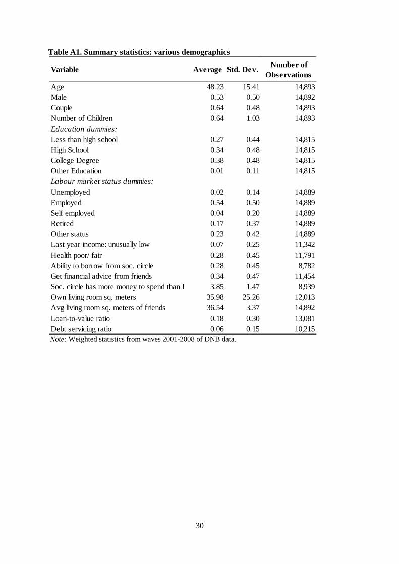
Appendix A. Definitions of Variables and Summary Statistics Types of Debt: Ability to borrow from social circle. Yes to “Are you currently in a position to borrow a substantial sum of money from family or friends?” (LENEN=1) Loans from social circle: Loans from family and friends. Collateralized loans: Debts on hire-purchase contracts; debts based on payment by installment; equity based loans; debts with mail-order firms; shops or other retail business; mortgages on main house, second house and other pieces of real estate. Outstanding uncollateralized debt: Private loans; extended lines of credit; study loans; credit card debts; other loans. Questions on characteristics of the social circle: The following questions concern your circle of acquaintances, that is, the people with whom you associate frequently, such as friends, neighbors, acquaintances, or maybe people at work. KENLTD. If you think of your circle of acquaintances, into which age category do MOST of these people go? Please select the answer that is closest to reality. Age (in years) is mostly: under 16; 16 – 20; 21 - 25; 26 - 30; 31 - 35; 36 - 40; 41 - 45; 46 - 50; 51 - 55; 56 - 60; 61 - 65; 66 - 70; 71 or over. KENHH. The people in your circle of acquaintances may live alone or share a household with other people (for example with a partner and children). Of how many persons do MOST households of your acquaintances consist? one person; two persons; three persons; four persons; five persons; six persons or more. KENINK. How much do you think is the AVERAGE total net income per year of those households? less than € 8,000 per year; € 8,000 – 9,500; € 9,500 – 11,000; € 11,000 – 13,000; € 13,000 – 16,000; € 16,000 – 20,000; € 20,000 – 28,000; € 28,000 – 38,000; € 38,000 – 50,000; € 50,000 – 75,000; € 75,000 or more; don’t know. KENOPL. Which level of education do MOST of your acquaintances have? primary education; junior vocational training; lower secondary education; secondary education/pre-university education; senior vocational training; vocational colleges/first year university education; university education. KENWERK. What kind of employment do MOST of your acquaintances have? self-employed; practicing a free profession; working in the family business; employed on a contractual basis; mostly no paid job. MANUUR (VROUWUUR). If you think of the MEN (WOMEN) among your acquaintances, how many hours per week do they work on average?

29

Other questions: Get financial advice from friends. When answering “parents, friends or acquaintances” to the following question: “What is your most important source of advice when you have to make important financial decisions for the household?” (ADVIES=1). Social circle has more money to spend than I. “Other people in my environment have more money to spend than I. Please indicate to what extent you agree or disagree” (SITUAT3: 1.totally disagree…7.totally agree). Last year income: unusually low. “Is the income your household earned in the past 12 months unusually high or low compared to the income you would expect in a ‘regular’ year, or is it regular?” (INKNORM= 1.“Unusually low”). Perceived lower bound on next period’s income. “What do you expect to be the LOWEST total net monthly income your household may realize in the next 12 months? (HOOG).

30

Table A1. Summary statistics: various demographics

Note: Weighted statistics from waves 2001-2008 of DNB data.

Variable Average Std. Dev. Number of Observations

Age 48.23 15.41 14,893Male 0.53 0.50 14,892Couple 0.64 0.48 14,893Number of Children 0.64 1.03 14,893Education dummies:Less than high school 0.27 0.44 14,815High School 0.34 0.48 14,815College Degree 0.38 0.48 14,815Other Education 0.01 0.11 14,815Labour market status dummies:Unemployed 0.02 0.14 14,889Employed 0.54 0.50 14,889Self employed 0.04 0.20 14,889Retired 0.17 0.37 14,889Other status 0.23 0.42 14,889Last year income: unusually low 0.07 0.25 11,342Health poor/ fair 0.28 0.45 11,791Ability to borrow from soc. circle 0.28 0.45 8,782Get financial advice from friends 0.34 0.47 11,454Soc. circle has more money to spend than I 3.85 1.47 8,939Own living room sq. meters 35.98 25.26 12,013Avg living room sq. meters of friends 36.54 3.37 14,892Loan-to-value ratio 0.18 0.30 13,081Debt servicing ratio 0.06 0.15 10,215

31

Table A2. Summary statistics: various economic indicators

Note: Weighted statistics from waves 2001-2008 of DNB data. Amounts refer to constant 2008 euro.

Variable Average Std. Dev. 25th perc Median 75th perc Number of obs

Avg. peer income 31,807 13,955 24,000 33,000 36,941 6,872Net hh income 27,617 23,638 15,943 24,687 35,886 10,031Net financial wealth 36,137 100,092 1,393 10,847 36,430 11,412Net real wealth 102,417 179,408 0 11,913 163,576 13,245Perceived lower bound on next period's income

17,500 36,683 2,134 14,434 26,387 11,049

32

Appendix B. Calculation of average marginal effects via Monte Carlo simulation

Given that marginal effects are non-linear functions of the estimated parameters, β̂ (either

from probit or tobit models), we compute their point estimates and standard errors via Monte

Carlo simulation (Train, 2003) by using the formula:

ββββ dfggE )()())(( ∫=

where ( )g β denotes the magnitude of interest and ( )f β the joint distribution of all the

elements in β. We implement this simulation estimator by drawing 500 times from the joint

distribution of the estimated vector of parameters β̂ under the assumption that it is

asymptotically normal with mean and variance-covariance matrix equal to the maximum

likelihood estimates. Then, for a given parameter draw j we generate the magnitude of

interest ˆ( )jg β . We first calculate this magnitude for each household in our sample, and then

calculate the average marginal effect as the weighted average of the effect across all

households in our sample, using survey weights.22 ( ( ))E g β We then estimate and its standard

error as the mean and standard deviation, respectively, of the distribution of ˆ( )jg β over all

parameter draws. Details on the formulae used to derive unconditional and conditional

marginal effects after the tobit estimation can be found in Green (2000, Chapter 22).

22 We do not evaluate marginal effects at sample means since this practice can lead to severely misleading results (see Train, 2003, pp. 33-34).

33

Appendix C. Further Robustness Checks

We performed a number of checks in addition to those presented in the main text in order to

ensure the consistency of our findings. First, about twenty percent of households answer

“don’t know” to the question regarding the perceived average income of their peers and thus

they are not used in our baseline regressions. To examine the sensitivity of our findings to the

inclusion of these missing observations we have re-estimated all our baseline models

presented in Tables 2, 3, and 4 and add a flag dummy to denote households answering that

they do not know the income of their peers. For these observations the missing income of the

peers is replaced by zeros. Estimated average marginal effects and associated standard errors

for the income of the peers from this larger sample of households are presented in Table C.1.

Notably, the estimated magnitudes across all specifications are very similar to those we

estimate in our baseline models.

Second, we experimented with different specifications that employ quartiles to model the

income of the peers and our results are robust to such transformations. Our results are also

insensitive to functional forms that use quartiles to model own income and/ or own financial

and real wealth.

Third, our modeling strategy of borrowing behavior is quite standard in household finance

literature and it is in line with life-cycle portfolio models in which households decide each

single period for the allocation of their resources and the amount of borrowing. Yet, one may

argue that for many households that are observed in the data with collateralized loans

outstanding in a given period, the decision to take up such loans (especially mortgages) is

quite binding and has been typically made many years prior to the interview. To examine the

sensitivity of our results to this issue, we have re-estimated our probit model for

collateralized loans focusing only on households that take up such loans (i.e., switch

borrowing status) during the period covered by our data. Specifically, we use the sample of

households without collateralized loans in 2001 (i.e., the initial observation period in our

sample) and estimate the probability of taking up such a loan in any of the subsequent seven

waves. This probit model conditions on the same set of covariates as the one used in our

baseline specification (presented in Table 3). The estimated marginal effect on the income of

the peers is 2 pp, significant at 1%, and contributes almost 20% to the unconditional

probability of taking up a collateralized loan in this sample. Thus, estimated effects on the

34

income of the peers from this ‘inflow’ sample are economically important and relatively

stronger to those we derive in our baseline specification.

Fourth, one might argue that the estimated effects of income of the peers on collateralized

loans are partly due to expectations about future housing market conditions. To that effect,

we have estimated specifications of collateralized debt behavior that take into account, apart

from peers’ income and expectations about next year’s own income, various expectations

regarding future conditions in housing and mortgage markets. In particular, we take into

account whether respondents expect housing prices to go up, whether they anticipate an

increase in mortgage interest rates, and whether they think that tax deductibility of mortgage

interest rates will be limited in the future. Results (available upon request) suggest a

significant negative relationship between an expected increase in mortgage interest rates and

collateralized debt, but they do not affect our baseline findings regarding the significant role

of income of peers or of expectations about next year’s own income (shown in Table 7, panel

A).

35

Table C.1. Effects of Peer Income (taking into account ‘do not know’ responses).

Note: Selected marginal effects from probit regressions modeling the probability of having a loan and marginal effects from tobit regressions on the log amount of the loan outstanding conditional on having such loan. Reported marginal effects are based on a 12,000 euro annual increase of peer income. Specifications in panels A, B, and C condition on the same set of covariates used in the baseline specifications in Tables 2, 3, and 4, respectively, and a flag dummy denoting households that answer ‘do not know’ to the peer income question. Standard errors are corrected for heteroscedasticity and clustered at the household level. ***,**,* denote significance at 1%, 5% and 10% respectively.

Marg. Eff. std. error Marg. Eff. std. error Marg. Eff. std. errorIHS(avg. peer income) 0.0256 0.0075 *** 0.0090 0.0039 ** 0.2796 0.1129 **

Log likelihood -3,414.9 -1,049.6 -1,892.7Number of Observations 6,375 7,405 7,405

Marg. Eff. std. error Marg. Eff. std. errorIHS(avg. peer income) 0.0416 0.0081 *** 0.4713 0.0827 ***

Log likelihood -3,799.9 -14,480.5Number of Observations 6,373 6,373

Marg. Eff. std. error Marg. Eff. std. errorIHS(avg. peer income) 0.0157 0.0056 *** 0.2307 0.0792 ***


Pr(Consumer Loans>0)E(log(Cons. Loans))|Cons.

Loans>0

Panel A. Loans from Social CirclePr(perceived ability to

borrow from social circle in the future>0)

Pr(Loans from social circle>0)

E(log(Loans from social circle))|Loans from social

circle>0

Panel B. Collateralized Loans

Pr(Collateralized Loans>0)E(log(Colat. Loans))|Colat.

Loans>0

Panel C. Consumer Loans

36

Table D.1: Auxiliary Regressions

Age 0.0219 0.0041 *** 0.0217 0.0039 *** 0.0228 0.0042 *** 0.0164 0.0074 ** 0.0187 0.0070 *** 0.0171 0.0074 **Age^2 -0.0002 0.0000 *** -0.0002 0.0000 *** -0.0002 0.0000 *** -0.0002 0.0001 ** -0.0002 0.0001 ** -0.0002 0.0001 **Male -0.0162 0.0192 -0.0260 0.0182 -0.0177 0.0191 0.0434 0.0306 0.0217 0.0281 0.0404 0.0307Couple 0.1841 0.0198 *** 0.1832 0.0191 *** 0.1824 0.0197 ***Numb of Children 0.0102 0.0081 0.0125 0.0078 0.0104 0.0081 0.0131 0.0117 0.0154 0.0111 0.0124 0.0119High School Education 0.2441 0.0232 *** 0.2469 0.0223 *** 0.2411 0.0234 *** 0.0853 0.0333 ** 0.0802 0.0315 ** 0.0836 0.0336 **College Degree 0.4321 0.0255 *** 0.4353 0.0245 *** 0.4275 0.0257 *** 0.1218 0.0357 *** 0.1169 0.0333 *** 0.1215 0.0359 ***Other Education 0.0000 0.0000 0.0000 0.0000 0.0000 0.0000 0.2069 0.0950 ** 0.0000 0.0000 0.1966 0.0968 **Employed 0.1141 0.0261 *** 0.1253 0.0246 *** 0.1145 0.0261 *** 0.0655 0.0366 * 0.0787 0.0339 ** 0.0631 0.0367 *Self employed 0.1137 0.0574 ** 0.1102 0.0541 ** 0.1126 0.0574 ** 0.0554 0.0822 0.0844 0.0758 0.0599 0.0827Retired 0.0653 0.0310 ** 0.0689 0.0285 ** 0.0672 0.0312 ** 0.0214 0.0505 0.0360 0.0461 0.0240 0.0510Unemployed 0.1255 0.0617 ** 0.1196 0.0604 ** 0.1289 0.0619 ** 0.1270 0.0866 0.1295 0.0814 0.1255 0.0873Last year income: unusually low -0.1352 0.0331 *** -0.1289 0.0315 *** -0.1330 0.0331 *** -0.1350 0.0558 ** -0.1365 0.0487 *** -0.1321 0.0555 **Health poor/ fair -0.0272 0.0170 -0.0207 0.0160 -0.0258 0.0169 -0.0323 0.0248 -0.0324 0.0235 -0.0312 0.0247IHS(net hh income) 0.0149 0.0029 *** 0.0129 0.0026 *** 0.0147 0.0029 *** 0.0176 0.0058 *** 0.0174 0.0053 *** 0.0177 0.0059 ***IHS(net fin wealth) 0.0031 0.0011 *** 0.0028 0.0011 *** 0.0029 0.0011 *** 0.0045 0.0018 ** 0.0048 0.0017 *** 0.0045 0.0018 **IHS(net real wealth) 0.0067 0.0017 *** 0.0074 0.0016 *** 0.0066 0.0017 *** 0.0062 0.0028 ** 0.0063 0.0025 ** 0.0063 0.0028 **Percv. ability to borrow from social circle in the future

0.0324 0.0159 ** 0.0368 0.0249

Get advice from soc. circle -0.0014 0.0150 0.0120 0.0236Regional dummiesYear dummiesConstant 9.7130 0.1136 *** 9.7379 0.1075 *** 9.6834 0.1165 *** 9.6186 0.2043 *** 9.5818 0.1937 *** 9.5922 0.2065 ***(avg. peer Educat. - own Educat.)*Regional empl. % in h tech 0.0380 0.0026 *** 0.0390 0.0025 *** 0.0377 0.0026 ***avg. peer Age (non fin. resp.) 0.0037 0.0020 * 0.0031 0.0019 0.0037 0.0020 *avg. peer Education (non fin. resp.) 0.0381 0.0056 *** 0.0379 0.0053 *** 0.0372 0.0056 ***F-statistic - instruments (p-value) 208.68 0.00 *** 250.80 0.00 *** 205.48 0.00 *** 23.65 0.00 *** 25.82 0.00 *** 22.69 0.00 ***Number of Observations 4,363 4,899 4,362 1,339 1,545 1,339

- - -

-

-yesyes

-

-yesyes

yesyes

-

-yesyes

yesyes

-

-yesyes

IV 1 IV 2(1) (2) (3) (4) (5) (6)

37

Table 1. Prevalence and Amount of Borrowing by Loan type

Note: Weighted statistics from waves 2001-2008 of DNB data. Amounts refer to constant 2008 euro.

Year Average 25th perc Median 75th perc2001 30.45% 4.87% 15,212 1,583 2,771 15,8322002 32.24% 4.96% 13,582 2,279 5,065 12,6622003 29.68% 4.26% 12,010 1,391 3,241 15,6892004 25.80% 3.92% 10,207 1,058 3,704 10,7832005 28.12% 4.47% 7,976 1,098 2,196 7,3202006 27.55% 3.73% 7,650 1,439 3,085 7,1972007 25.99% 3.72% 8,488 1,829 3,810 7,1122008 28.10% 3.49% 9,422 1,500 3,000 7,900Total 28.31% 4.16% 10,638 1,519 3,313 10,282

Average 25th perc Median 75th perc2001 37.81% 105,038 44,857 83,118 131,9342002 43.22% 113,177 45,760 89,288 139,5122003 43.12% 113,921 44,298 90,757 146,9402004 40.96% 110,673 46,562 92,065 145,4052005 41.25% 118,971 51,238 100,384 156,8512006 40.69% 117,246 49,353 100,763 159,3702007 41.02% 132,048 59,944 111,760 181,8642008 40.92% 132,920 61,750 120,000 180,000Total 41.15% 117,926 48,620 98,293 156,664

Average 25th perc Median 75th perc2001 22.24% 11,451 956 4,486 11,6102002 24.62% 9,448 843 4,659 12,3442003 25.86% 13,030 918 4,415 13,4872004 25.09% 11,315 835 4,021 11,7942005 19.13% 14,957 1,045 4,273 12,5482006 18.64% 11,267 853 4,138 12,2872007 20.57% 11,196 889 3,835 11,3792008 20.33% 12,008 680 3,750 11,206Total 22.09% 11,793 875 4,181 12,155

Panel A. Loans from Social Circle



Conditional amounts outstanding

Conditional amounts outstandingPrevalence (%)

Prevalence (%)

Perceived ability to borrow from social circle in the future (%)

Prevalence (%)

Conditional amounts outstanding

38

Table 2. Loans from Social Circle

Note: Marginal effects from probit regressions modeling the probability of having an outstanding loan from friends and marginal effects from tobit regressions on the log amount of loan outstanding conditional on having such loan. All marginal effects have been averaged across households in the sample using survey weights. The marginal effects for peer income are based on a 12,000 euro annual increase of the underlying variable. The marginal effects for household income, financial, and real wealth are calculated assuming a one standard deviation increase of the underlying covariates. Standard errors are corrected for heteroscedasticity and clustered at the household level. ***,**,* denote significance at 1%, 5% and 10% respectively.

Marg. Eff. std. error Marg. Eff. std. error Marg. Eff. std. errorIHS(avg. peer income) 0.0225 0.0079 *** 0.0084 0.0040 ** 0.2653 0.1169 **Age -0.0088 0.0009 *** -0.0016 0.0005 *** -0.0509 0.0165 ***Male 0.0442 0.0219 ** 0.0043 0.0087 0.1467 0.2628Couple 0.0352 0.0233 -0.0097 0.0113 -0.2920 0.3156Numb of Children -0.0032 0.0110 -0.0015 0.0049 -0.0581 0.1499High School Education 0.0698 0.0267 *** 0.0258 0.0119 ** 0.7756 0.3462 **College Degree 0.0783 0.0262 *** 0.0070 0.0112 0.2473 0.3682Other Education 0.2578 0.1181 ** 0.0000 0.0000 0.0000 0.0000Employed -0.0053 0.0323 0.0126 0.0113 0.3841 0.3433Self employed 0.0313 0.0533 0.0518 0.0315 1.4181 0.7126 **Retired -0.0584 0.0342 * -0.0005 0.0148 -0.0254 0.4845Unemployed -0.1210 0.0519 ** -0.0035 0.0214 -0.1968 0.6611Last year income: unusually low -0.0787 0.0301 *** 0.0325 0.0186 * 0.8419 0.4174 **Health poor/ fair -0.0472 0.0202 ** -0.0026 0.0097 -0.1001 0.2979IHS(net hh income) 0.0025 0.0042 0.0003 0.0017 0.0083 0.0530IHS(net fin wealth) 0.0248 0.0068 *** -0.0141 0.0031 *** -0.6676 0.1274 ***IHS(net real wealth) 0.0052 0.0071 0.0055 0.0038 0.1733 0.1101Regional dummiesYear dummies

Log likelihood -2,529.6 -820.2 -1,502.4Number of Observations 4,524 5,074 5,074

IHS(avg. peer income) 0.0878 0.0267 ***F-statistic from Auxilliary Regression (p-value ) 208.68 0.00 *** 250.80 0.00 *** 250.80 0.00 ***Exogeneity Test (p-value ) 6.08 0.01 ** 1.25 0.26 1.39 0.24Number of Observations 4,363 4,899 4,899

IHS(avg. peer income) 0.1677 0.0406 ***F-statistic from Auxilliary Regression (p-value ) 23.65 0.00 *** 25.82 0.00 *** 25.82 0.00 ***Sargan Hansen Test for overidentificat. (p-value ) 0.37 0.55 4.99 0.03 ** 4.99 0.03 **Exogeneity Test (p-value ) 6.83 0.01 *** 2.04 0.15 2.04 0.15Number of Observations 1,339 1,545 1,545

Probit Tobit

IV 2

IV 1

Pr(perceived ability to borrow from social circle in

the future>0)

Pr(Loans from social circle>0)

yes yesyes yes

E(log(Loans from soc. circle))|Loans from soc.

circle>0

yesyes

39

Table 3. Collateralized Loans

Note: Marginal effects from probit regressions modeling the probability of having an outstanding collateralized loan and marginal effects from tobit regressions on the log amount of collateralized loan outstanding conditional on having such loan. See notes in Table 2.

Marg. Eff. std. error Marg. Eff. std. errorIHS(avg. peer income) 0.0444 0.0085 *** 0.4984 0.0862 ***Age -0.0016 0.0011 -0.0280 0.0119 **Male 0.0001 0.0249 -0.0007 0.2959Couple 0.1709 0.0266 *** 1.8652 0.2661 ***Numb of Children 0.0126 0.0122 0.1059 0.1192High School Education 0.0205 0.0291 0.2296 0.3182College Degree 0.0728 0.0299 ** 0.8510 0.3338 **Other Education 0.0199 0.1477 0.3260 1.8588Employed 0.0807 0.0342 ** 0.8935 0.3551 **Self employed 0.0894 0.0567 1.0961 0.5685 *Retired 0.0312 0.0386 0.5009 0.4379Unemployed 0.0122 0.0723 0.1606 0.8299Last year income: unusually low -0.0977 0.0360 *** -1.2901 0.3688 ***Health poor/ fair -0.0104 0.0231 -0.1803 0.2347IHS(net hh income) 0.0138 0.0042 *** 0.1387 0.0366 ***IHS(net fin wealth) 0.0024 0.0066 0.0500 0.0601IHS(net real wealth) 0.0709 0.0092 *** 0.3858 0.0540 ***Perceived ability to borrow from soc. circle in the future 0.0091 0.0210 0.0149 0.2219Get advice from soc. circle -0.0296 0.0191 -0.4001 0.2152 *Regional dummiesYear dummies


F-statistic from Auxilliary Regression (p-value ) 205.48 0.00 *** 205.48 0.00 ***Exogeneity Test (p-value ) 2.12 0.15 2.06 0.15Number of Observations 4,362 4,362

F-statistic from Auxilliary Regression (p-value ) 22.69 0.00 *** 22.69 0.00 ***Sargan Hansen Test for overidentification (p-value ) 0.17 0.50 0.17 0.50Exogeneity Test (p-value ) 1.92 0.17 1.92 0.17Number of Observations 1,339 1,339

IV 2


Loans>0

Probit Tobit

IV 1

yes yesyes yes

40

Table 4. Consumer Loans

Note: Marginal effects from probit regressions modeling the probability of having a consumer loan and marginal effects from tobit regressions on the log amount of consumer loan outstanding conditional on having such loan. See notes in Table 2.

Marg. Eff. std. error Marg. Eff. std. errorIHS(avg. peer income) 0.0158 0.0058 *** 0.2385 0.0810 ***Age -0.0021 0.0007 *** -0.0276 0.0095 ***Male 0.0107 0.0157 0.2180 0.1916Couple 0.0562 0.0160 *** 0.6868 0.2313 ***Numb of Children 0.0001 0.0071 0.0323 0.1008High School Education 0.0175 0.0187 0.2084 0.2572College Degree 0.0137 0.0200 0.0965 0.2634Other Education 0.1243 0.0919 1.0343 0.9973Employed 0.0164 0.0203 0.0757 0.2563Self employed 0.0296 0.0349 0.1830 0.4699Retired 0.0033 0.0266 -0.1311 0.4001Unemployed 0.0475 0.0523 0.5328 0.5808Last year income: unusually low 0.0726 0.0307 ** 0.8331 0.2996 ***Health poor/ fair 0.0230 0.0144 0.2769 0.1937IHS(net hh income) 0.0042 0.0032 0.0808 0.0484 *IHS(net fin wealth) -0.1962 0.0042 *** -3.4979 0.0535 ***IHS(net real wealth) 0.0018 0.0051 0.0073 0.0887Perceived ability to borrow from soc. circle in the future -0.0098 0.0141 -0.1470 0.1798Get advice from soc. circle -0.0262 0.0126 ** -0.3693 0.1707 **Regional dummiesYear dummies



F-statistic from Auxilliary Regression (p-value ) 22.69 0.00 *** 22.69 0.00 ***Sargan Hansen Test for overidentification (p-value ) 1.28 0.26 1.28 0.26Exogeneity Test (p-value ) 0.00 0.97 0.00 0.97Number of Observations 1,339 1,339

IV 1

IV 2

yes yes

Probit Tobit

Pr(Consumer Loans>0) E(log(Cons. Loans))|Cons. Loans>0

yes yes

41

Table 5. Placebo Regressions

Note: Selected marginal effects from probit regressions modeling the probability of having a formal loan and marginal effects from tobit regressions on the log amount of the loan outstanding conditional on having such loan. Peer income is that of a randomly assigned household belonging to the same year, age, education, gender cell as the respondent’s social circle. The marginal effects for peer income are based on a 12,000 euro annual increase of the underlying variable. Specifications in panel A (panel B) condition on the same set of covariates used in the baseline specifications in Table 3 (Table 4). Standard errors are corrected for heteroscedasticity and clustered at the household level. ***,**,* denote significance at 1%, 5% and 10% respectively.

Marg. Eff. std. error Marg. Eff. std. errorIHS(avg. peer income) -0.0061 0.0057 -0.0031 0.0710

Marg. Eff. std. error Marg. Eff. std. errorIHS(avg. peer income) -0.0025 0.0043 0.2340 0.1979

Pr(Consumer Loans>0)E(log(Cons. Loans))|Cons.

Loans>0

Panel A. Collateralized Loans

Panel B. Consumer Loans


Loans>0

42

Table 6. Asymmetric Effects of Peer Income

Note: Selected marginal effects from probit regressions modeling the probability of having a loan and marginal effects from tobit regressions on the log amount of the loan outstanding conditional on having such loan. Presented marginal effects are based on a 12,000 euro annual increase of peer income. Specifications in panels A, B, and C condition on the same set of covariates used in the baseline specifications in Tables 2, 3, and 4, respectively. Standard errors are corrected for heteroscedasticity and clustered at the household level. ***,**,* denote significance at 1%, 5% and 10% respectively.

Marg. Eff. std. error Marg. Eff. std. error Marg. Eff. std. errorIHS(own income)-IHS(avg. peer income)>0 0.0116 0.0054 ** 0.0009 0.0023 0.0254 0.0654IHS(own income)-IHS(avg. peer income)<0 0.0111 0.0045 ** 0.0062 0.0024 *** 0.2056 0.0692 ***

Marg. Eff. std. error Marg. Eff. std. errorIHS(own income)-IHS(avg. peer income)>0 -0.0041 0.0060 -0.0054 0.0682IHS(own income)-IHS(avg. peer income)<0 0.0366 0.0052 *** 0.3184 0.0423 ***

Marg. Eff. std. error Marg. Eff. std. errorIHS(own income)-IHS(avg. peer income)>0 0.0034 0.0037 0.0516 0.0531IHS(own income)-IHS(avg. peer income)<0 0.0104 0.0033 *** 0.1642 0.0494 ***

Pr(Consumer Loans>0)

Pr(perceived ability to borrow from social circle in

the future>0)Pr(Loans from social circle>0)

E(log(Loans from social circle))|Loans from social

circle>0

E(log(Cons. Loans))|Cons. Loans>0

Panel A. Loans from Social Circle




Loans>0

43

Table 7. Living Standards, Perceived Ability of the Social Circle to Spend, and Expected Future Own Income

Note: Selected marginal effects from probit regressions modeling the probability of having a formal loan and marginal effects from tobit regressions on the log amount of the loan outstanding conditional on having such loan. The marginal effects for peer income are based on a 12,000 euro annual increase of the underlying variable. The marginal effects for average sq. meters of friends, own square meters, and expected income next period are calculated assuming a one SD increase of the underlying covariates. Specifications in panel A (panel B) also condition on the set of covariates used in the baseline specifications in Table 3 (Table 4). Standard errors are corrected for heteroscedasticity and clustered at the household level. ***,**,* denote significance at 1%, 5% and 10% respectively.

Marg. Eff. std. error Marg. Eff. std. errorIHS(avg. peer income) 0.0352 0.0088 *** 0.4097 0.0906 ***Avg sq. meters of friends 0.0215 0.0104 ** 0.2841 0.1244 **Own sq. meters 0.0423 0.0172 ** 0.3796 0.1337 ***IHS(perceived lower bound on next period’s income) 0.0452 0.0128 *** 0.4828 0.1267 ***Log likelihood -2,436.4 -9,875.9Number of Observations 4,206 4,206

Marg. Eff. std. error Marg. Eff. std. errorIHS(avg. peer income) 0.0127 0.0061 ** 0.1838 0.0881 **Soc. circle has more money to spend than I 0.0123 0.0049 ** 0.1820 0.0633 ***IHS(perceived lower bound on next period’s income) 0.0012 0.0092 0.0258 0.1313Log likelihood -1,361.9 -4,443.3Number of Observations 3,669 3,669

Prob(Consumer credit>0) E(log(Cons. credit))|Cons. credit>0Probit Tobit

Panel B. Consumer Loans

Panel A. Collateralized Loans

Prob(Collateralized Debt>0) E(log(Colat. Debt))|Colat. Debt>0Probit Tobit

44

Table 8. Peer Income and Over-indebtedness

Note: Marginal effects from tobit regressions on measures of financial distress. All marginal effects have been averaged across households in the sample using survey weights. The marginal effects for peer income are based on a 12,000 euro annual increase of the underlying variable. The marginal effects for household income, financial, and real wealth are calculated assuming a one standard deviation increase of the underlying covariates. Standard errors are corrected for heteroscedasticity and clustered at the household level. ***,**,* denote significance at 1%, 5% and 10% respectively.

Marg. Eff. std. error Marg. Eff. std. errorIHS(avg. peer income) 0.0371 0.0058 *** 0.0102 0.0034 ***Age -0.0040 0.0008 *** -0.0005 0.0005Male -0.0044 0.0174 0.0103 0.0102Couple 0.1115 0.0175 *** 0.0267 0.0102 ***Numb of Children 0.0092 0.0075 0.0008 0.0043High School Education 0.0011 0.0188 0.0202 0.0109 *College Degree 0.0434 0.0190 ** 0.0301 0.0116 ***Other Education 0.0547 0.1228 0.0457 0.0797Employed 0.0707 0.0206 *** 0.0363 0.0149 **Self employed 0.0911 0.0370 ** 0.0263 0.0240Retired 0.0467 0.0254 * 0.0202 0.0162Unemployed 0.0158 0.0474 0.0326 0.0303Last year income: unusually low -0.0933 0.0207 *** -0.0478 0.0115 ***Health poor/ fair -0.0161 0.0142 -0.0082 0.0082IHS(net hh income) 0.0106 0.0030 *** 0.0172 0.0017 ***IHS(net fin wealth) 0.0103 0.0051 ** 0.0015 0.0025IHS(net real wealth) -0.0037 0.0067 0.0218 0.0037 ***Perceived ability to borrow from soc. circle in the future -0.0096 0.0125 -0.0033 0.0082Get advice from soc. circle -0.0310 0.0135 ** -0.0096 0.0079Regional dummiesYear dummies



F-statistic from Auxilliary Regression (p-value ) 22.65 0.00 *** 21.79 0.00 ***Sargan Hansen Test for overidentification (p-value ) 0.95 0.33 0.59 0.44Exogeneity Test (p-value ) 1.13 0.29 0.11 0.74Number of Observations 1,331 948

IV 2

E(Loan to Value Ratio) E(Debt Servicing Ratio)

Tobit Tobit

IV 1

yes yesyes yes

CFS Working Paper Series: No. Author(s) Title

2012/04 Nikolaus Hautsch Ruihong Huang

On the Dark Side of the Market: Identifying and Analyzing Hidden Order Placements

2012/03 Volker Wieland Tobias Cwik Gernot J. Müller Sebastian Schmidt Maik Wolters

A New Comparative Approach to Macroeconomic Modeling and Policy Analysis

2012/02 Andrej Gill Uwe Walz

Going Public – Going Private The Case of VC-backed Firms

2012/01 Laura Moretti Inflation Targeting and Product Market Deregulation

2011/31 Neil A. Doherty Christian Laux Alexander Muermann

Insuring Non-Verifiable Losses

2011/30 Konstantinos Voutsinas Richard Werner

New Evidence on the Effectiveness of ‘Quantitative Easing’ in Japan

2011/29 Victor Lyonnet Richard Werner

The Lessons from QE and Other ‘Unconventional’ Monetary Policies – Evidence from the Bank of England

2011/28 Dimitris Christelis Loretti I. Dobrescu Alberto Motta

Early Life Conditions and Financial Risk–Taking in Older Age

2011/27 Dimitris Christelis Dimitris Georgarakos Tullio Jappelli

Wealth Shocks, Unemployment Shocks and Consumption in the Wake of the Great Recession

2011/26 Richard A. Werner The Unintended Consequences of the Debt - - - Will Increased Government Expenditure Hurt the Economy?

Copies of working papers can be downloaded at http://www.ifk-cfs.de

dimitris georgarakos,michael haliassos, and giacomo pasini · * we would like to thank rob alessie,...

Documents