digital image processing chapter 3: image enhancement in the spatial domain 15 june 2007 digital...

Digital Image ProcessingChapter 3:

Image Enhancement in the Spatial Domain

15 June 2007

Digital Image ProcessingChapter 3:

Image Enhancement in the Spatial Domain

15 June 2007

Spatial Domain Spatial Domain

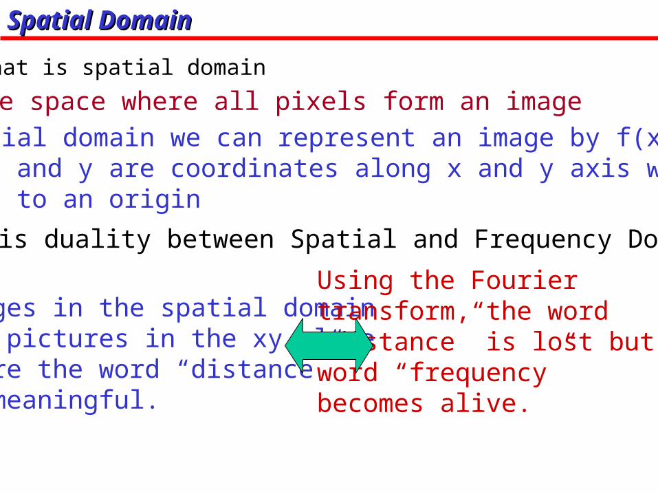
What is spatial domain

The space where all pixels form an image

In spatial domain we can represent an image by f(x,y)where x and y are coordinates along x and y axis with respect to an origin

There is duality between Spatial and Frequency Domains

Images in the spatial domain are pictures in the xy planewhere the word “distance” is meaningful.

Using the Fourier transform, the word “distance” is lost but the word “frequency” becomes alive.

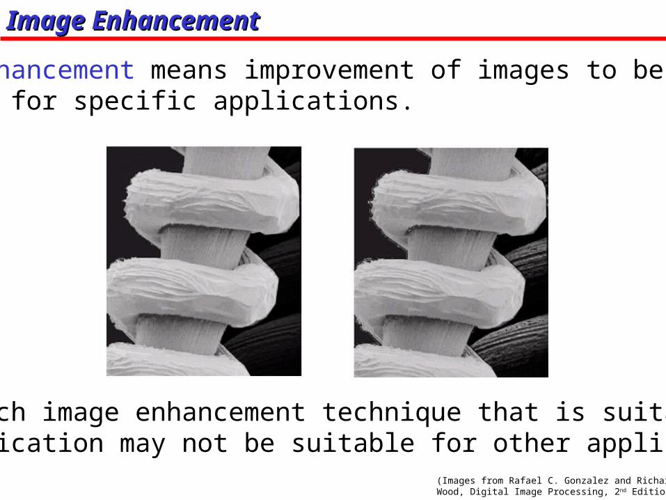
Image EnhancementImage Enhancement

Image Enhancement means improvement of images to be suitable for specific applications. Example:

Note: each image enhancement technique that is suitable for one application may not be suitable for other applications.

(Images from Rafael C. Gonzalez and Richard E. Wood, Digital Image Processing, 2nd Edition.

Image Enhancement ExampleImage Enhancement Example

Original image Enhanced image using Gamma correction


= Image enhancement using processes performed in the Spatial domain resulting in images in the Spatial domain.We can written as

Image Enhancement in the Spatial DomainImage Enhancement in the Spatial Domain

( , ) ( , )g x y T f x y

where f(x,y) is an original image, g(x,y) is an output and T[ ] is a function defined in the area around (x,y)

Note: T[ ] may have one input as a pixel value at (x,y) only ormultiple inputs as pixels in neighbors of (x,y) depending in each function. Ex. Contrast enhancement uses a pixel value at (x,y) only for an input while smoothing filte use several pixels around (x,y) as inputs.

Types of Image Enhancement in the Spatial DomainTypes of Image Enhancement in the Spatial Domain

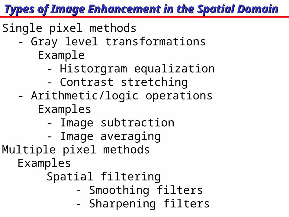
- Single pixel methods- Gray level transformations Example

- Historgram equalization- Contrast stretching

- Arithmetic/logic operations Examples

- Image subtraction- Image averaging

- Multiple pixel methodsExamples

Spatial filtering - Smoothing filters- Sharpening filters

Gray Level TransformationGray Level Transformation

Transforms intensity of an original image into intensity of an output image using a function:

( )s T r

where r = input intensity and s = output intensity

Example: Contrast enhancement


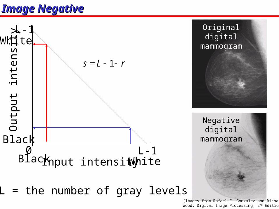
Image NegativeImage Negative

White

Black

Input intensity

Out

put i

nten

sity

Originaldigital

mammogram

1s L r

L = the number of gray levels

0 L-1

L-1

Negativedigital

mammogram


Black White

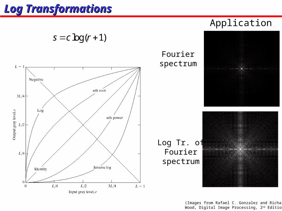
Log TransformationsLog Transformations

Fourierspectrum

Log Tr. ofFourier

spectrum

log( 1)s c r Application


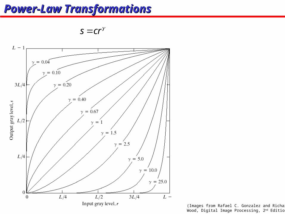
Power-Law TransformationsPower-Law Transformations

s cr


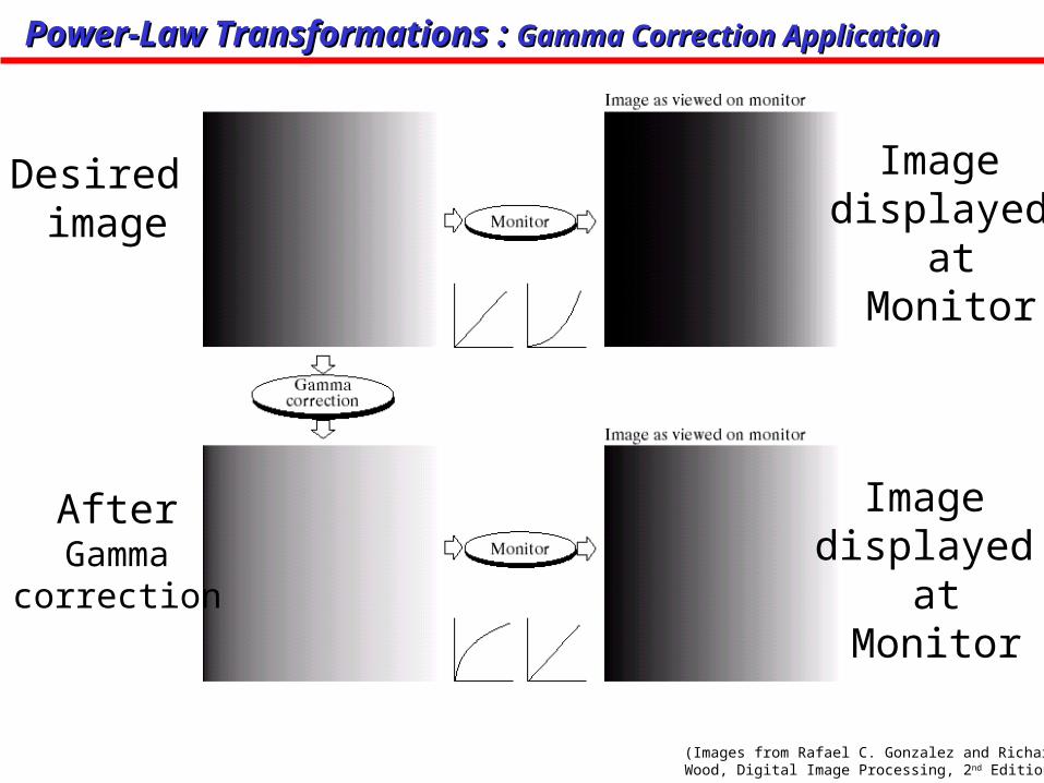
Power-Law Transformations : Power-Law Transformations : Gamma Correction ApplicationGamma Correction Application

Desired image

Image displayed

atMonitor

AfterGamma

correction


Image displayed

atMonitor


MRI Image after Gamma Correction



Ariel imagesafter GammaCorrection


Contrast StretchingContrast Stretching

Before contrast enhancement

After

Contrast means the difference between the brightest and darkest intensities


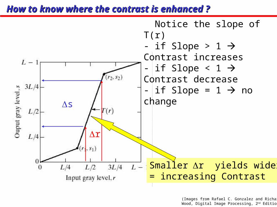
How to know where the contrast is enhanced ? How to know where the contrast is enhanced ?

Notice the slope of T(r)- if Slope > 1 Contrast increases- if Slope < 1 Contrast decrease- if Slope = 1 no change

r

s

Smallerr yields wider s= increasing Contrast


Gray Level SlicingGray Level Slicing


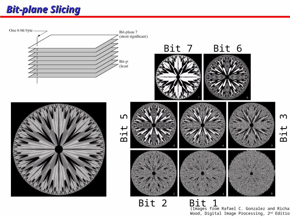
Bit-plane SlicingBit-plane Slicing

Bit 7 Bit 6

Bit 2 Bit 1

Bit

5

Bit

3


HistogramHistogram

Histogram = Graph of population frequencies

0

2

4

6

8

10

A B+ B C+ C D+ D F

No. ofStudents

Grades of the course 178 xxx

Histogram of an ImageHistogram of an Image

( )k kh r n

จำ��นว

น pi

xel

จำ��นว

น pi

xel

= graph of no. of pixels vs intensities


Bright image has histogram on the right

Dark image has histogram on the left

Histogram of an Image (cont.)Histogram of an Image (cont.)

low contrast image has narrow histogram


high contrast image has wide histogram

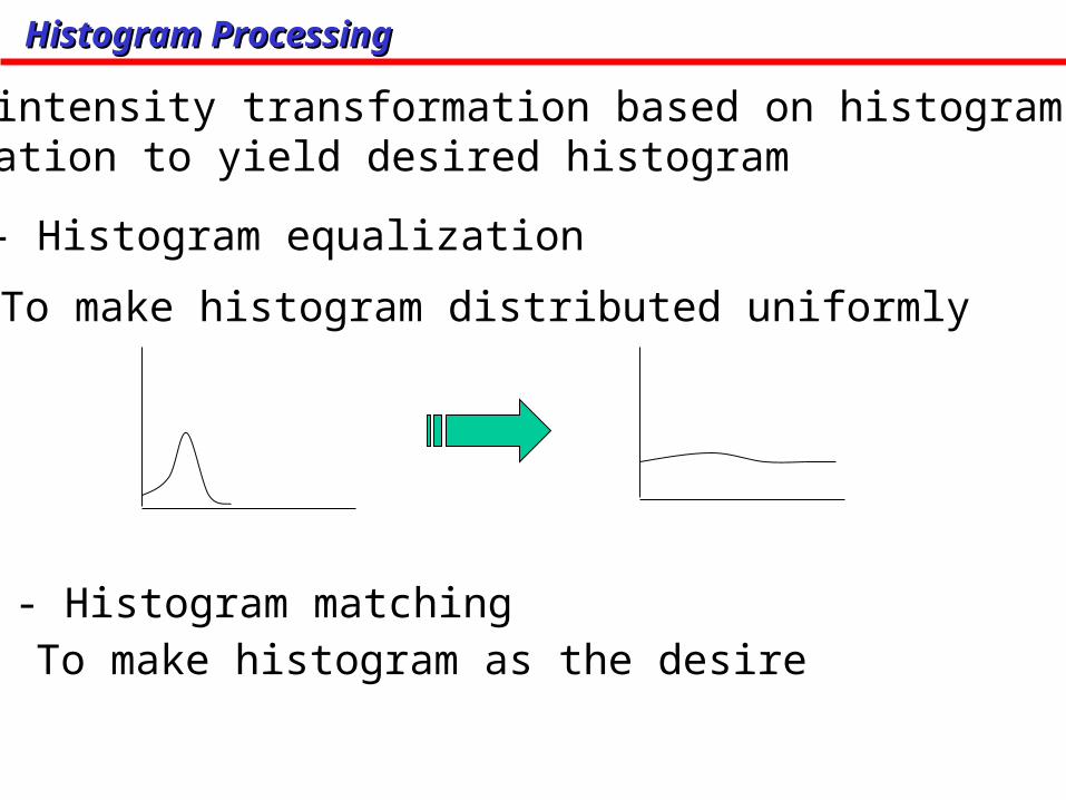
Histogram ProcessingHistogram Processing

= intensity transformation based on histogram information to yield desired histogram

- Histogram equalization

- Histogram matching

To make histogram distributed uniformly

To make histogram as the desire

Monotonically Increasing FunctionMonotonically Increasing Function

= Function that is only increasing or constant

)(rTs

Properties of Histogram processing function

1. Monotonically increasing function

2. 10for 1)(0 rrT

Probability Density FunctionProbability Density Function

and relation between s and r is

Histogram is analogous to Probability Density Function (PDF) which represent density of population

Let s and r be Random variables with PDF ps(s) and pr(r ) respectively

)(rTs

We get

ds

drrpsp rs )()(

r

r dwwprTs0

)()(

Histogram EqualizationHistogram Equalization

Let

We get

1)(

1)(

)(

1)(

1)()()(

0

rp

rp

dr

dwwpd

rp

drds

rpds

drrpsp

rrr

r

r

rrs

!


Formula in the previous slide is for a continuous PDF

For Histogram of Digital Image, we use

k

j

j

k

jjrkk

N

n

rprTs

0

0

)()(

nj = the number of pixels with intensity = jN = the number of total pixels

Histogram Equalization ExampleHistogram Equalization Example

Intensity # pixels

0 20

1 5

2 25

3 10

4 15

5 5

6 10

7 10

Total 100

Accumulative Sum of Pr

20/100 = 0.2

(20+5)/100 = 0.25

(20+5+25)/100 = 0.5

(20+5+25+10)/100 = 0.6

(20+5+25+10+15)/100 = 0.75

(20+5+25+10+15+5)/100 = 0.8

(20+5+25+10+15+5+10)/100 = 0.9

(20+5+25+10+15+5+10+10)/100 = 1.0

1.0

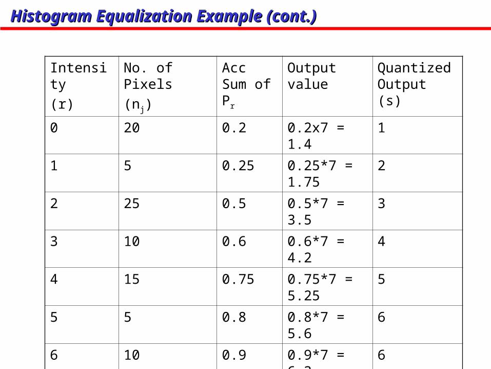
Histogram Equalization Example (cont.)Histogram Equalization Example (cont.)

Intensity

(r)

No. of Pixels

(nj)

Acc Sum of Pr

Output value Quantized Output (s)

0 20 0.2 0.2x7 = 1.4 1

1 5 0.25 0.25*7 = 1.75 2

2 25 0.5 0.5*7 = 3.5 3

3 10 0.6 0.6*7 = 4.2 4

4 15 0.75 0.75*7 = 5.25 5

5 5 0.8 0.8*7 = 5.6 6

6 10 0.9 0.9*7 = 6.3 6

7 10 1.0 1.0x7 = 7 7

Total 100

Histogram Equalization (cont.)Histogram Equalization (cont.)


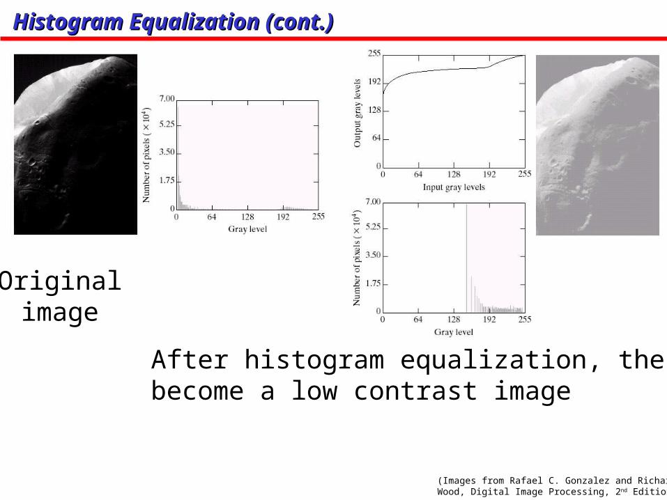
Histogram Equalization (cont.)Histogram Equalization (cont.)

Originalimage

After histogram equalization, the imagebecome a low contrast image


Histogram MatchingHistogram Matching : Algorithm: Algorithm

r

r dwwprTs0

)()(

Concept : from Histogram equalization, we have

We get ps(s) = 1

We want an output image to have PDF pz(z)Apply histogram equalization to pz(z), we get

z

z duupzGv0

)()( We get pv(v) = 1

Since ps(s) = pv(v) = 1 therefore s and v are equivalent

Therefore, we can transform r to z by

r T( ) s G-1( ) z

To transform image histogram to be a desired histogram

Histogram Matching : Algorithm (cont.)Histogram Matching : Algorithm (cont.)

s = T(r) v = G(z)

z = G-1(v)

1

2

3

4


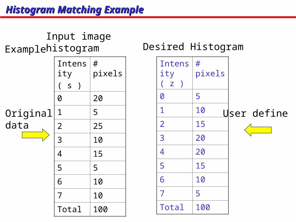
Histogram Matching ExampleHistogram Matching Example

Intensity

( s )

# pixels

0 20

1 5

2 25

3 10

4 15

5 5

6 10

7 10

Total 100

Input imagehistogram

Intensity ( z )

# pixels

0 5

1 10

2 15

3 20

4 20

5 15

6 10

7 5

Total 100

Desired HistogramExample

User defineOriginaldata

r (nj) Pr s

0 20 0.2 1

1 5 0.25 2

2 25 0.5 3

3 10 0.6 4

4 15 0.75 5

5 5 0.8 6

6 10 0.9 6

7 10 1.0 7

Histogram Matching Example Histogram Matching Example (cont.)(cont.)

1. Apply Histogram Equalization to both tables

z (nj) Pz v

0 5 0.05 0

1 10 0.15 1

2 15 0.3 2

3 20 0.5 4

4 20 0.7 5

5 15 0.85 6

6 10 0.95 7

7 5 1.0 7

sk = T(rk) vk = G(zk)

r s

0 1

1 2

2 3

3 4

4 5

5 6

6 6

7 7

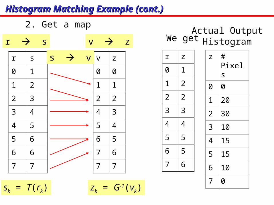
Histogram Matching Example Histogram Matching Example (cont.)(cont.)

2. Get a map

v z

0 0

1 1

2 2

4 3

5 4

6 5

7 6

7 7

sk = T(rk) zk = G-1(vk)

r s v z

s v

We get

r z

0 1

1 2

2 2

3 3

4 4

5 5

6 5

7 6

z # Pixels

0 0

1 20

2 30

3 10

4 15

5 15

6 10

7 0

Actual Output Histogram

Histogram Matching Example (cont.)Histogram Matching Example (cont.)

Desired histogram

Transfer function

Actual histogram


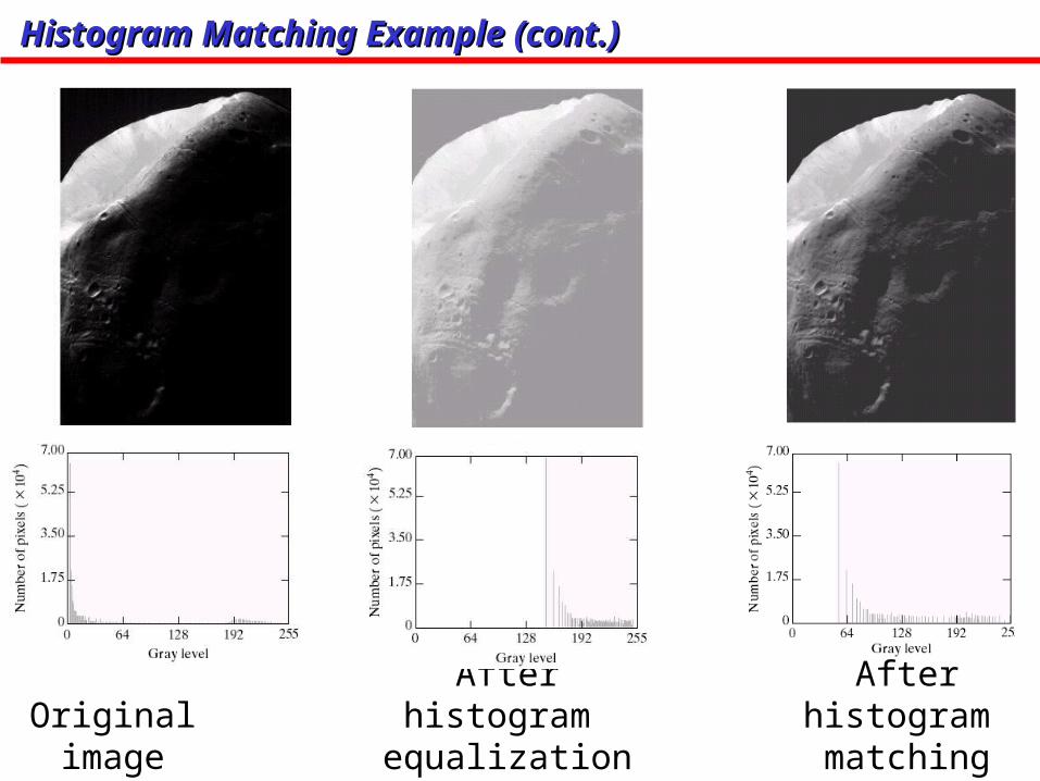
Histogram Matching Example (cont.)Histogram Matching Example (cont.)

Originalimage

Afterhistogram

equalization

Afterhistogram matching

Local Enhancement : Local Histogram EqualizationLocal Enhancement : Local Histogram Equalization

Concept: Perform histogram equalization in a small neighborhood

Orignal image After Hist Eq.After Local Hist Eq.In 7x7 neighborhood


Local Enhancement : Local Enhancement : Histogram Statistic for Image EnhancementHistogram Statistic for Image Enhancement

We can use statistic parameters such as Mean, Variance of Local area for image enhancement

Image of tungsten filament taken usingAn electron microscope

In the lower right corner, there is afilament in the background which isvery dark and we want this to be brighter.

We cannot increase the brightness of the whole image since the white filament will be too bright.


Local EnhancementLocal Enhancement

Example: Local enhancement for this task

otherwise ),(

and when),(),( 210

yxf

MkDkMkmyxfEyxg GsGGs xyxy

Original imageLocal Variance

image Multiplication

factor


Local EnhancementLocal Enhancement

Output image


Logic OperationsLogic Operations

AND

OR

Result Region of Interest

Image maskOriginalimage

Application:Crop areas of interest


Arithmetic Operation: SubtractionArithmetic Operation: Subtraction

Error image

Application: Error measurement


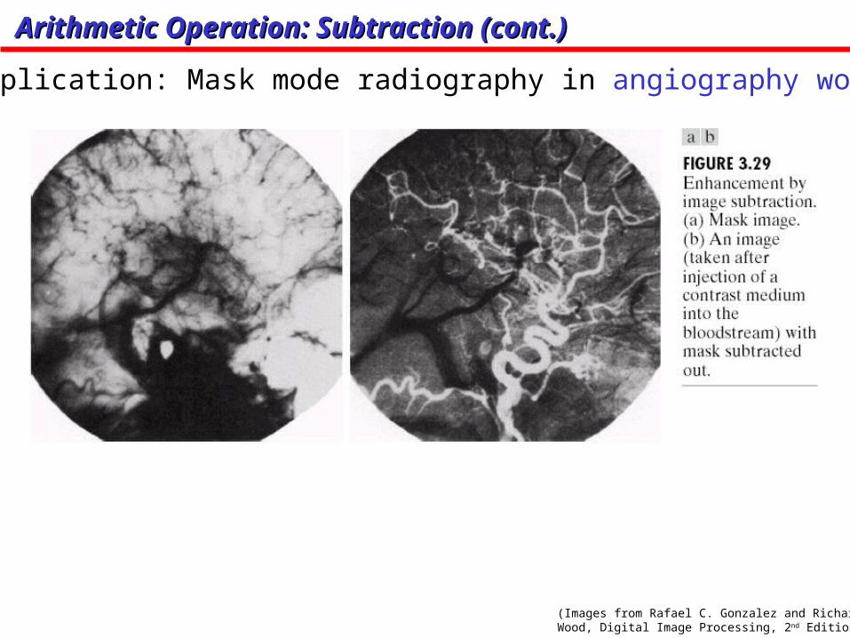
Arithmetic Operation: Subtraction (cont.)Arithmetic Operation: Subtraction (cont.)

Application: Mask mode radiography in angiography work


Arithmetic Operation: Image AveragingArithmetic Operation: Image Averaging

Application : Noise reduction

),(),(

1yxyxg

K

Averaging results in reduction of Noise variance

),(),(),( yxyxfyxg Degraded image

(noise)Image averaging

K

ii yxg

Kyxg

1

),(1

),(


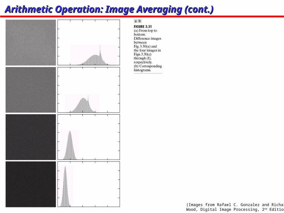
Arithmetic Operation: Image Averaging (cont.)Arithmetic Operation: Image Averaging (cont.)


Sometime we need to manipulate values obtained from neighboring pixels

Example: How can we compute an average value of pixelsin a 3x3 region center at a pixel z?

4

4

67

6

1

9

2

2

2

7

5

2

26

4

4

5

212

1

3

3

4

2

9

5

7

7

35 8222

Pixel z

Image

Basics of Spatial FilteringBasics of Spatial Filtering

4

4

67

6

1

9

2

2

2

7

5

2

26

4

4

5

212

1

3

3

4

2

9

5

7

7

35 8222

Pixel z

Step 1. Selected only needed pixels

4

67

6

9

1

3

3

4……

……

Basics of Spatial Filtering (cont.)Basics of Spatial Filtering (cont.)

4

67

6

9

1

3

3

4……

……

Step 2. Multiply every pixel by 1/9 and then sum up the values

19

16

9

13

9

1

69

17

9

19

9

1

49

14

9

13

9

1

y

1 1

1

1

1

1

1

1

19

1

X

Mask orWindow orTemplate


Question: How to compute the 3x3 average values at every pixels?

4

4

67

6

1

9

2

2

2

7

5

2

26

4

4

5

212

1

3

3

4

2

9

5

7

7

Solution: Imagine that we havea 3x3 window that can be placedeverywhere on the image

Masking Window


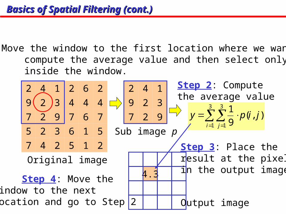
4.3

Step 1: Move the window to the first location where we want to compute the average value and then select only pixels inside the window.

4

4

67

6

1

9

2

2

2

7

5

2

26

4

4

5

212

1

3

3

4

2

9

5

7

7

Step 2: Computethe average value

3

1

3

1

),(9

1

i j

jipy

Sub image p

Original image

4 1

9

2

2

3

2

9

7

Output image

Step 3: Place theresult at the pixelin the output image

Step 4: Move the window to the next location and go to Step 2


The 3x3 averaging method is one example of the mask operation or Spatial filtering.

The mask operation has the corresponding mask (sometimes called window or template).

The mask contains coefficients to be multiplied with pixelvalues.

w(2,1) w(3,1)

w(3,3)

w(2,2)

w(3,2)

w(3,2)

w(1,1)

w(1,2)

w(3,1)

Mask coefficients

1 1

1

1

1

1

1

1

19

1

Example : moving averaging

The mask of the 3x3 moving average filter has all coefficients = 1/9


The mask operation at each point is performed by:1. Move the reference point (center) of mask to the location to be computed 2. Compute sum of products between mask coefficients and pixels in subimage under the mask.

p(2,1)

p(3,2)p(2,2)

p(2,3)

p(2,1)

p(3,3)

p(1,1)

p(1,3)

p(3,1)

……

……

Subimage

w(2,1) w(3,1)

w(3,3)

w(2,2)

w(3,2)

w(3,2)

w(1,1)

w(1,2)

w(3,1)

Mask coefficients

N

i

M

j

jipjiwy1 1

),(),(

Mask frame

The reference pointof the mask


The spatial filtering on the whole image is given by:

1. Move the mask over the image at each location.

2. Compute sum of products between the mask coefficeintsand pixels inside subimage under the mask.

3. Store the results at the corresponding pixels of the output image.

4. Move the mask to the next location and go to step 2until all pixel locations have been used.


Examples of Spatial Filtering Masks

Examples of the masks

Sobel operators

0 1

1

0

0

2

-1

-2

-1

-2 -1

1

0

2

0

-1

0

1

x

P

compute toy

P

compute to

1 1

1

1

1

1

1

1

19

1

3x3 moving average filter

-1 -1

-1

8

-1

-1

-1

-1

-19

1

3x3 sharpening filter

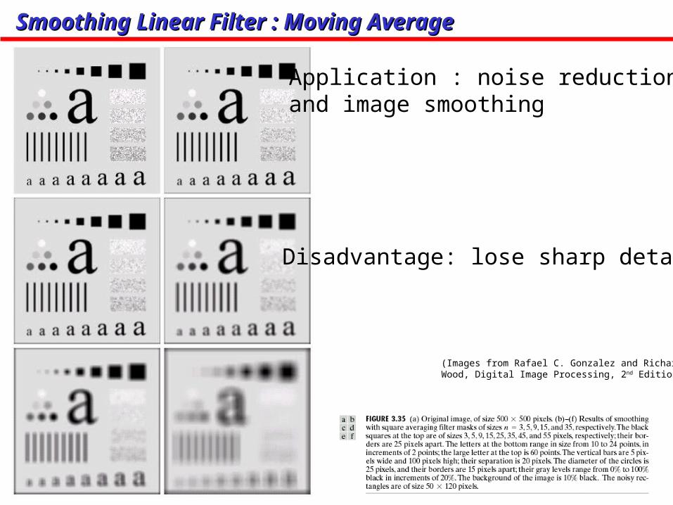
Smoothing Linear Filter : Moving AverageSmoothing Linear Filter : Moving Average

Application : noise reductionand image smoothing

Disadvantage: lose sharp details


Smoothing Linear Filter (cont.)Smoothing Linear Filter (cont.)


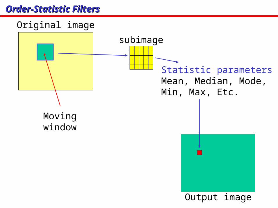
Order-Statistic FiltersOrder-Statistic Filters

subimage

Original image

Moving window

Statistic parametersMean, Median, Mode, Min, Max, Etc.

Output image

Order-Statistic Filters: Median FilterOrder-Statistic Filters: Median Filter


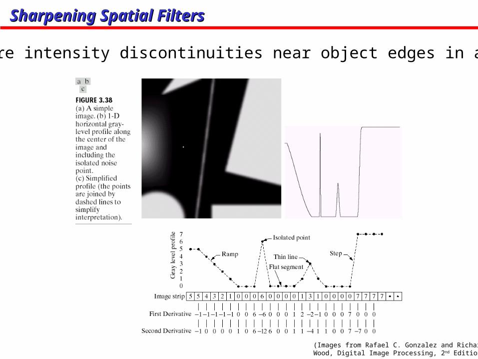
Sharpening Spatial FiltersSharpening Spatial Filters

There are intensity discontinuities near object edges in an image


Laplacian Sharpening : How it worksLaplacian Sharpening : How it works

20 40 60 80 100 120 140 160 180 200

0

0.5

1

0 50 100 150 2000

0.1

0.2

0 50 100 150 200-0.05

0

0.05

Intensity profile

1st derivative

2nd derivative

p(x)

dx

dp

2

2

dx

pd

Edge

0 50 100 150 200-0.5

0

0.5

1

1.5

0 50 100 150 200-0.5

0

0.5

1

1.5

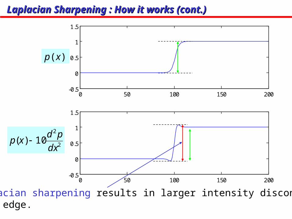
Laplacian Sharpening : How it works (cont.)Laplacian Sharpening : How it works (cont.)

2

2

10)(dx

pdxp

Laplacian sharpening results in larger intensity discontinuity near the edge.

p(x)

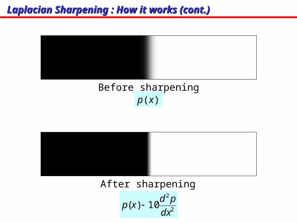
Laplacian Sharpening : How it works (cont.)Laplacian Sharpening : How it works (cont.)

2

2

10)(dx

pdxp

p(x)Before sharpening

After sharpening

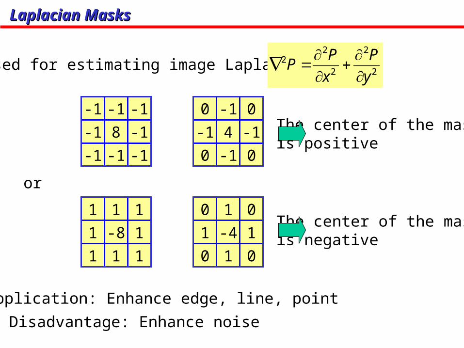
Laplacian MasksLaplacian Masks

-1 -1

-1

8

-1

-1

-1

-1

-1

-1 0

0

4

-1

-1

0

-1

0

1 1

1

-8

1

1

1

1

1

1 0

0

-4

1

1

0

1

0

Application: Enhance edge, line, point

Disadvantage: Enhance noise

Used for estimating image Laplacian 2

2

2

22

y

P

x

PP

or

The center of the mask is positive

The center of the mask is negative

Laplacian Sharpening ExampleLaplacian Sharpening Example

p P2

P2 PP 2


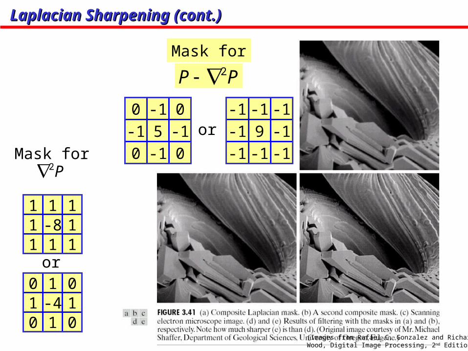
Laplacian Sharpening (cont.)Laplacian Sharpening (cont.)

PP 2Mask for

1 1

1-81

1111

-1 -1

-1

9

-1

-1

-1

-1

-1

-1 0

0

5

-1

-1

0

-1

0

1 0

0-41

1010

or

Mask forP2

or


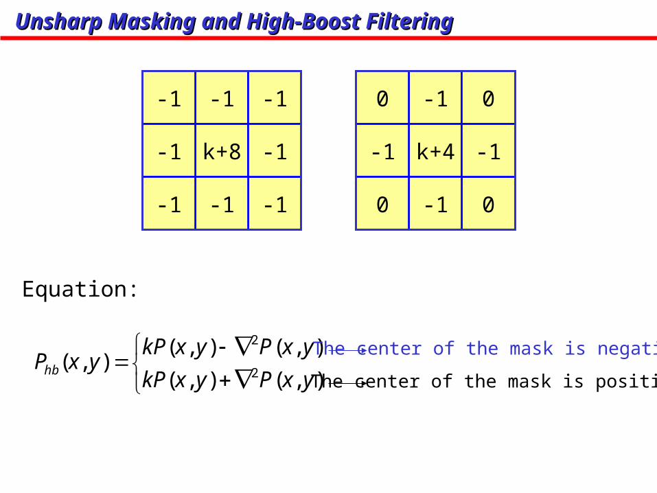
Unsharp Masking and High-Boost FilteringUnsharp Masking and High-Boost Filtering

-1 -1

-1

k+8

-1

-1

-1

-1

-1

-1 0

0

k+4

-1

-1

0

-1

0

Equation:

),(),(

),(),(),(

2

2

yxPyxkP

yxPyxkPyxPhb

The center of the mask is negative

The center of the mask is positive

Unsharp Masking and High-Boost Filtering (cont.)Unsharp Masking and High-Boost Filtering (cont.)


First Order DerivativeFirst Order Derivative

20 40 60 80 100 120 140 160 180 2000

0.5

1

0 50 100 150 200-0.2

0

0.2

0 50 100 150 2000

0.1

0.2

Intensity profile

1st derivative

2nd derivative

p(x)

dx

dp

dx

dp

Edges

First Order Partial Derivative:First Order Partial Derivative:

Sobel operators

0 1

1

0

0

2

-1

-2

-1

-2 -1

1

0

2

0

-1

0

1x

P

compute toy

P

compute to

Px

P

y

P

First Order Partial Derivative: Image GradientFirst Order Partial Derivative: Image Gradient

22

y

P

x

PP

Gradient magnitude

A gradient image emphasizes edges(Images from Rafael C. Gonzalez and Richard E. Wood, Digital Image Processing, 2nd Edition.

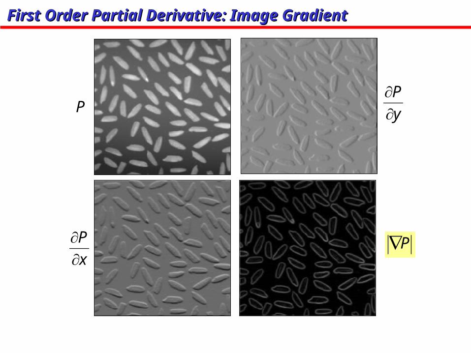
First Order Partial Derivative: Image GradientFirst Order Partial Derivative: Image Gradient

P

x

P

y

P

P

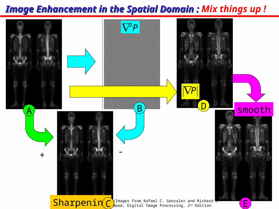
Image Enhancement in the Spatial Domain : Image Enhancement in the Spatial Domain : Mix things up !

+ -

A

P2

Sharpening

P

smoothB

EC

D


EC

MultiplicationF

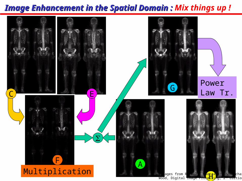
Image Enhancement in the Spatial Domain : Image Enhancement in the Spatial Domain : Mix things up !

A

G

H

PowerLaw Tr.


digital image processing chapter 3: image enhancement in the spatial domain 15 june 2007 digital...

Documents