laboratory

DIGIT AL COMPUTER APPLICATION IN PROCESS CONTROL

M. F. ABD-EL-BARY AND SRIRAM CHARI New Jersey Institute of Technology Newark, NJ 07102

WITH THE RAPID DEVELOPMENT and extensive use of Direct Digital Control (DDC) in in­

dustry, smaller versions of digital computers equipped with laboratory modules are being utilized increasingly in undergraduate Process Control laboratories to train chemical engineers in the theory and practice of digital control. It was pointed out by Waller [1], however, that the thrust of process control teaching is still directed toward very basic facts only, and that old text­books were being used to a large extent. Newer textbooks and laboratory experiments should, therefore, emphasize computers and digital systems.

One of the chief reasons for the popularity of digital computers is the "amplifier-limitation"

M. F. Abd-EI-Bary is an Assistant Professor at the New Jersey

Institute of Technology. He holds degrees from Alexandria Un iversity,

MIT, and Lehigh University. He has a strong interest in the area of digital control. His research work is primarily in the fleld of water and air pollution. (L)

Sriram Chari is an MBA student at the Harvard Business School. He has a B.S.ChE from Indian Institute of Technology, Delhi, and an M.S.ChE from New Jersey Institute of Technology. He was a Shift

Engineer at Swadeshi Polytex Limited in Ghaziabad, India, before working on th is project as a Teaching Assistant at NJIT. (R)

118

C.ONCENTRA.T li:0 S,,t,, \. T S01..VTIOl'I

V{\ )

PUl'\E W,,_TEr:;i -. {t.)

•

CONCENTll .... T!ON ruc.01:10ER -CONTllOLLER A.ND Tll;.6,N!,Q UCEJl:

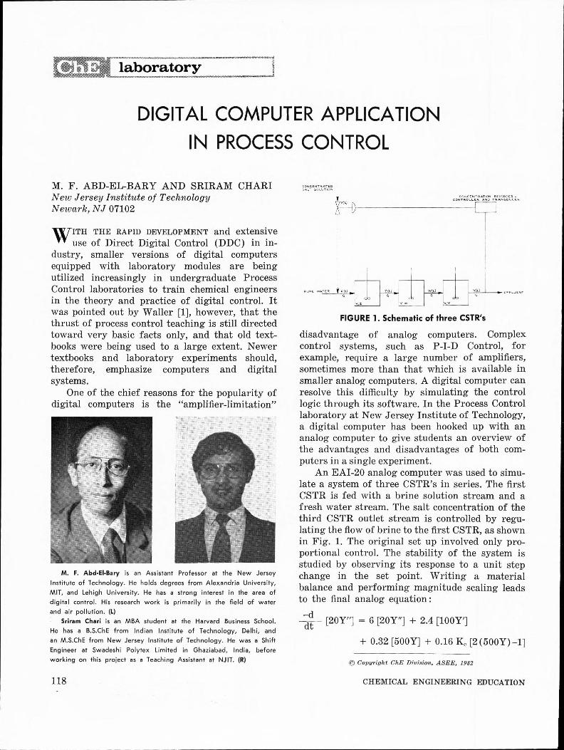
FIGURE 1. Schematic of three CSTR's

disadvantage of analog computers. Complex control systems, such as P-I-D Control, for example, require a large number of amplifiers, sometimes more than that which is available in smaller analog computers. A digital computer can resolve this difficulty by simulating the control logic through its software. In the Process Control laboratory at New Jersey Institute of Technology, a digital computer has been hooked up with an analog computer to give students an overview of the advantages and disadvantages of both com­puters in a single experiment.

An EAI-20 analog computer was used to simu­late a system of three CSTR's in series. The first CSTR is fed with a brine solution stream and a fresh water stream. The salt concentration of the third CSTR outlet stream is controlled by regu­lating the flow of brine to the first CSTR, as shown in Fig. 1. The original set up involved only pro­portional control. The stability of the system is studied by observing its response to a unit step change in the set point. Writing a material balance and performing magnitude scaling leads to the final analog equation :

~~ [20Y"] = 6 [20Y"] + 2.4 [lO0Y']

+ 0.32 [500Y] + 0.16 K0 [2(500Y) - 1]

© Copyright ChE Division, ASEE, 1982

CHEMICAL ENGINEERING EDUCATION

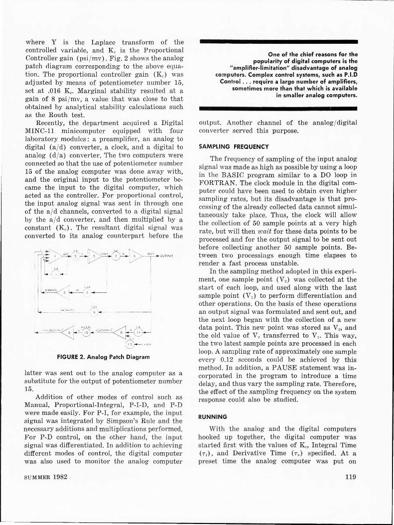
where Y is the Laplace transform of the controlled variable, and Kc is the Proportional Controller gain (psi / mv). Fig. 2 shows the analog patch diagram corresponding to the above equa­tion. The proportional controller gain (Kc) was adjusted by means of potentiometer number 15, set at .016 Kc. Marginal stability resulted at a gain of 8 psi / mv, a value that was close to that obtained by analytical stability calculations such as the Routh test.

Recently, the department acquired a Digital MINC-11 minicomputer equipped with four laboratory modules: a preamplifier, an analog to digital (a / d) converter, a clock, and a digital to analog (d / a) converter. The two computers were connected so that the use of potentiometer number 15 of the analog computer was done away with, and the original input to the potentiometer be­came the input to the digital computer, which acted as the controller. For proportional control, the input analog signal was sent in through one of the a / d channels, converted to a digital signal by the a / d converter, and then multiplied by a constant (Kc). The resultant digital signal was converted to its analog counterpart before the

r~•-::c:~~~~,3 - ,o,; ~,-.~~OUTPUT I cu, I 1---:,...,._,

I '-

t I~~: ~·.__J ' '- -I •

FIGURE 2. Analog Patch Diagram

latter was sent out to the analog computer as a substitute for the output of potentiometer number 15.

Addition of other modes of control such as Manual, Proportional-Integral, P-I-D, and P-D were made easily. For P-I, for example, the input signal was integrated by Simpson's Rule and the necessary additions and multiplications performed. For P-D control, on the other hand, the input signal was differentiated. In addition to achieving different modes of control, the digital computer was also used to monitor the analog computer

SUMMER 1982

One of the chief reasons for the popularity of digital computers is the

"amplifier-limitation" disadvantage of analog computers. Complex control systems, such as P.I.D

Control ... require a large number of amplifiers, sometimes more than that which is available

in smaller analog computers.

output. Another channel of the analog/ digital converter served this purpose.

SAMPLING FREQUENCY

The frequency of sampling of the input analog signal was made as high as possible by using a loop in the BASIC program similar to a DO loop in FORTRAN. The clock module in the digital com­puter could have been used to obtain even higher sampling rates, but its disadvantage is that pro­cessing of the already collected data cannot simul­taneously take place. Thus, the clock will allow the collection of 50 sample points at a very high rate, but will then wait for these data points to be processed and for the output signal to be sent out before collecting another 50 sample points. Be­tween two processings enough time elapses to render a fast process unstable.

In the sampling method adopted in this experi­ment, one sample point (V2) was collected at the start of each loop, and used along with the last sample point (V1 ) to perform differentiation and other operations. On the basis of these operations an output signal was formulated and sent out, and the next loop began with the collection of a new data point. This new point was stored as V 2, and the old value of V 2 transferred to V 1 • This way, the two latest sample points are processed in each loop. A sampling rate of approximately one sample every 0.12 seconds could be achieved . by this method. In addition, a PA USE statement. was in­corporated in the program to introduce a time delay, and thus vary the sampling rate. Therefore, the effect of the sampling frequency on the system response could also be studied.

RUNNING

With the analog and the digital computers hooked up together, the digital computer was started first with the values of Kc, Integral Time (Tr), and Derivative Time ( 7 0 ) specified. At a preset time the analog computer was put on

119

.•-. ....-- system response · _.,...set point

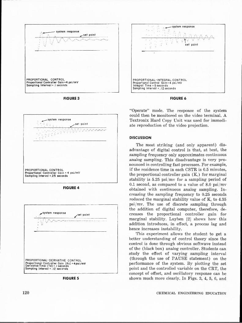
PROPORTIONAL CONTROL Proportional Controller Gain =4 psi/mV Sam pl ino lnterva I= . I seconds

FIGURE 3

. ....--system response

--. ----

/set point

PROPORTIONAL CONTROL Proportional Controller . Gain~ 4 psi/mV Sampling Interval =.25 seconds

FIGURE4

._;system response /set point

.. ..... ._,_ ____ ... ··· ... ,.•···· ...... • •,, _____ , ..........•...... \ -. •.•·········· .. ·-.-· ... ··-··.-····• .. ·.-·•.-·•·-···-,

· . ..-

PROPORTIONAL-DERIVATIVE CONTROL Proportional Controller Gain (Kc) =4psi/mV Derivative Time (Td) = .I seconds Sampling Interval= .12 seco~ds

FIGURE 5

120

.. -system response

.. ~ . · .. .- \ --·

set point

PROPORTIONAL -INTEGRAL CONTROL Proportional Control Goin= 4 psi/mV Integral Time= 5 seconds Sampling Interval= . 12 seconds

FIGURE 6

·.r -.,:

"Operate" mode. The response of the system could then be monitored on the video terminal. A Textronix Hard Copy Unit was used for immedi­ate reproduction of the video projection.

DISCUSSION

The most striking (and only apparent) dis­advantage of digital control is that, at best, the sampling frequency only approximates continuous analog sampling. This disadvantage is very pro­nounced in controlling fast processes. For example, if the residence time in each CSTR is 0.5 minutes, the proportional controller gain (Kc) for marginal stability is 5.25 psi /mv for a sampling period of 0.1 second, as compared to a value of 8.0 psi /mv obtained with continuous analog sampling. In­creasing the sampling frequency to 0.25 seconds reduced the marginal stability value of K c to 4.35 psi /mv. The use of discrete sampling through the addition of digital computer, therefore, de­creases the proportional controller gain for marginal stability. Luyben [2] shows how this addition introduces, in effect, a process lag and hence increases instability.

This experiment allows the student to get a better understanding of control theory since the control is done through obvious softwave instead of the (black box) analog controller. Students can study the effect of varying sampling interval (through the use of PAUSE statement) on the performance of the system. By plotting the set point and the controlled variable on the CRT, the concept of offset, and oscillatory response can be shown much more clearly. In Figs. 3, 4, 5, 6, and

CHEMICAL ENGINEERING EDUCATION

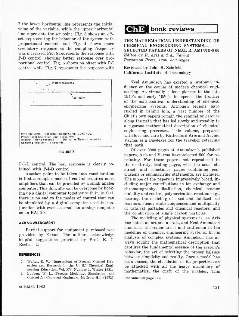
7 the lower horizontal line represents the initial value of the variable, while the upper horizontal line represents the set point. Fig. 3 shows an off­set, representing the behavior of the system with proportional control, and Fig. 4 shows more oscillatory response as the sampling frequency was increased. Fig. 5 represents the response with P-D control, showing better response over pro­portional control. Fig. 6 shows no offset with P-I control while Fig. 7 represents the response with

_:·. . / system response

' -· . ··- , -• .... _. __ ....... -.---.--~

\ . set point

PROPORTIONAL INTEGRAL-DERIVATIVE CONTROL Proportional Controller Goin = 4 psi / mV . Integral Time=5 seconds Derivative Time =.I seconds Sampling Interval= . 12 seconds

FIGURE 7

P-I-D control. The best response is clearly ob­tained with P-I-D control.

Another point to be taken into consideration is that a complex mode of control requires more amplifiers than can be provided by a small analog computer. This difficulty can be overcome by hook­ing up a digital computer together with it. In fact, there is no end to the modes of control that can be simulated by a digital computer used in con­junction with even as small an analog computer as an EAI-20.

ACKNOWLEDGMENT

Partial support for equipment purchased was provided by Exxon. The authors acknowledge helpful suggestions provided by Prof. E. C. Roche. •

REFERENCES

1. Waller, K. V., "Impressions of Process Control Edu­cation and Research in the U. S." Chemical Engi­neering Education, Vol. XV, Number 1, Winter 1981.

2. Luyben, W. L., Process Modeling, Simulation, and Control for Chemical Engineers, McGraw-Hill (1973).

SUMMER 1982

g} ;j pl book reviews

THE MATHEMATICAL UNDERSTANDING OF CHEMICAL ENGINEERING SYSTEMS­SELECTED PAPERS OF NEAL R. AMUNDSON Edited by R. Aris and A. Varma Pergamon Press, 1980. 830 pages

Reviewed by John H. Seinfeld California Institute of Technology

Neal Amundson has exerted a profound in­fluence on the course of modern chemical engi­neering. As virtually a lone pioneer in the late 1940's and early 1950's, he opened the frontier of the mathematical understanding of chemical engineering systems. Although legions have rushed in behind him, a vast number of the Chief's own papers remain the seminal milestones along the path that has led slowly and steadily to a rigorous mathematical description of chemical engineering processes. This volume, prepared with love and care by Rutherford Aris and Arvind Varma, is a Baedeker for the traveller retracing that path.

Of over 2000 pages of Amundson's published papers, Aris and Varma have selected 800 for re­printing. For those papers not reproduced in their entirety, leading pages, with the usual ab­stract, and sometimes pages containing con­clusions or summarizing statements, are included. The scope of the papers is impressively broad, in­cluding major contributions in ion exchange and chromatography, distillation, chemical reactor stability and control, polymerization reaction engi­neering, the modeling of fixed and fluidized bed reactors, steady state uniqueness and multiplicity of catalyst particles and chemical reactors, and the combustion of single carbon particles.

The modeling of physical systems is, as Aris has noted, an art and a craft, and Neal Amundson stands as the senior artist and craftsman in the modeling of chemical engineering systems. In his analysis of complex systems Amundson has al­ways sought the mathematical description that captures the fundamental essence of the system's behavior, the art of selecting the proper balance between simplicity and reality. Once a model has been chosen, the elucidation of its properties can be attacked with all the heavy machinery of mathematics, the craft of the modeler. This

Continued on page 125.

121