did freemasonry help solve the common good … · did freemasonry help solve the common good ... an...
TRANSCRIPT

Did Freemasonry Help Solve the Common Good
Problem?
An Examination of the Historical Expansion of
American Education in the Western United States
Daniel Egel
INITAL DRAFT: March 18, 2009
THIS DRAFT: May 5, 2010
Abstract
This paper examines the role that American Freemasonry played in the historical
expansion of the American educational system. I find evidence that 19th century
Freemasonry had a significant positive impact on educational enrollment during and
after the rapid rise of the ‘common school’ in the late 19th century. And in what is a
striking example of the ‘path dependence’ of social institutions, I show that this effect
persisted through the expansion of American high schools in the 1910s-1940s even after
the waning of the influence of this organization. I provide evidence that Freemasonry’s
impact was particularly significant in areas that were the most heterogeneous - both
ethnically and religiously. This, combined with the the further observation that areas
with more Freemasons had higher levels of local taxation, suggests that Freemasonry
helped communities overcome the common good problem. I provide evidence against
potential reverse causality by demonstrating that Freemasons did not tend to migrate
to areas with existing public education systems. Further, by exploiting a panel data set
of enrollment data, I provide evidence that unobserved heterogeneity and endogeneity
are not driving the observed relationship. In a voting model augmented to allow for
altruism I demonstrate the plausibility of these results. In particular I show how a
relatively small number of Freemasons could affect the equilibrium provision of public
education and why it is unsurprising to find that the impact of Freemasonry is larger
in more heterogeneous areas.
1

Very Preliminary - Please Do Not Cite 2
1 Introduction
Public education, an essential component of development, is under-provided in most devel-
oping societies. Though a public education system benefits all, communities are typically
unwilling to fund a system that is very costly, benefits only a minority of the population at
any one time and provides benefits unequally (Poterba 1997). In this way, public education
suffers from the classic “common good” problem.
During the 19th century, communities throughout the United States systematically
overcame this common good problem facing public education. Despite strong opposition
from a variety of groups who opposed public education for either financial or ideological
reasons, locally based, locally funded and locally administered public education systems be-
came widespread through this, then, developing nation (Black and Sokoloff 2006).1 These
local initiatives were the basis of the development of the most comprehensive public edu-
cation system of the era, which functioned almost entirely without the involvement of the
national government. Understanding the factors that allowed, and encouraged, communities
throughout the United States to overcome the difficulties in the provision of universal public
education has become a central strand in the historical education literature.
Previous studies have proposed a variety of mechanisms to explain the rapid spread of
public education during the 19th century. Many studies have pointed to the importance of
economic factors, such as the onset of industrialization or changing labor market conditions
that lowered the cost of education.2 Others have argued for the importance of religious
faith, social organizations such as labor organizations or urbanization in explaining this
spread.3 However, few previous studies have considered the potential role that American
Freemasonry played in the development of public education in the United States, despite
the general knowledge that many of the central figures in the education movement were
Freemasons and that Freemasonry was likely the most influential social organization in the
United States during this period.
The provision of free primary and higher education was indeed a central tenet of 19th
century American Freemasonry. Freemasonry, a voluntaristic secret society that attracted
and accepted men of all backgrounds, is well known for its prominence among national
politicians and businessmen. Though many of the activities of this organization are shrouded
1See also Cubberley (1920) and Soltow and Stevens (1981) that are mentioned by in footnote 3 of Blackand Sokoloff (2006).
2Black and Sokoloff (2006) and Go and Lindert (2008) are two recent examples.3See Boli, Ramirez, and Meyer (1985) and Black and Sokoloff (2006) as examples. Another interesting
argument offered by Black and Sokoloff (2006) (p. 73), particularly in light of the region considered here, isthat “residents of western states” were somehow different and that their pioneer attitude played an importantrole in the development of local public education.
Very Preliminary - Please Do Not Cite 3
in secrecy and mystery, their support for public education was quite open. Indeed, these men,
who were committed to the American ideals of equality and opportunity for all, believed that
education offered the means for individuals to obtain this equality and opportunity. This was
famously argued by perhaps the most celebrated and influential Freemason of the period,
Albert Pike:
“Equality has an organ; – gratuitious and obligatory instrution. We must beginwith the right to the alphabet. The primary school obligatory upon all; the highschool offered to all. Such is the law. From the same school for all springs equalsociety.” (Pike 1871, p.44)4
Here I argue that Freemasonry played an important role in supporting the expansion of
education in the United States. In particular, three characteristics of 19th century American
Freemasonry can explain its efforts and success in overcoming the public good problem
and encouraging the development of public education. The first of these characteristics is
that education, and in particular universal and free public education, was one of the most
important political issues during this time for American Freemasons. The second is that the
Freemason organization was particularly effective at developing relationships between men
of different backgrounds, and these relationships were often stronger than those found within
church organizations or even families. Third, Freemasons were particularly well suited for
finding political for causes that they supported as they were very politically active and often
dominated state legislatures and other political offices.
In order to understand how Freemasons could affect the equilibrium level of taxation
and public education I develop a public good voting model following Epple and Romano
(1996). As education in the United States throughout the nineteenth was funded locally,
and the major impediment to the development of education during this period was the
inability of local communities to levy taxes to generate the needed resources to build and fund
schools, understanding how Freemasonry could have affected political decisions is essential.
Augmenting these authors’ model to allow for the altruistic behavior of these Freemasons
(as suggested above) leads to three testable predictions:
1. Communities with Freemasonry are likely to have better educational outcomes than
other similar communities. The size of this impact, in addition to the probability that
there will be an impact, is increasing in the size of the local Freemason population.
2. The impact of Freemasonry will be larger in areas with greater heterogeneity. As
Freemasonry was inclusive and accepting of individuals from nearly all religions and
4This quotation was drawn from Fox (1997).

Very Preliminary - Please Do Not Cite 4
ethnicities, and allowed the development of strong relationships through mutual partic-
ipation in secretive rituals and traditions, Freemasonry would be particularly effective
in socially or ethnically heterogeneous areas where the common good problem is more
severe.
3. Areas with more Freemasons would have higher taxes and in particular higher local
taxes. This follows from the fact that the development of a public education required
the development of local taxation systems.
The analysis throughout this paper relies on two new sources of data. The first is data
on the number of Freemasons per county for 24 states of the Western United States during
the 1850-1900 period. Freemason data was collected decennially, to match the socioeconomic
data available in the census, and the lodge level data was aggregated to the county-level for
compatibility with the available economic data. The second source of data is a panel of
counties for the Western United States that allows for the panel data analysis employed in
this study. As county definitions changed frequently during this period, a panel data set
was constructed by creating county aggregates which represent a geographical area that is
constant over time.
In examining the relationship between Freemasonry and the development of American
education I explore two possible types of impact. First, I focus on measuring the poten-
tial contemporaneous impact of Freemasonry on primary public education in the late 19th
century. This period corresponds to the time in which Freemasonry’s influence in society
was likely most pronounced, and a time in which Freemasonry and public education were
spreading rapidly throughout the United States.
Second, I examine the potential long-term impact of Freemasonry by looking at the
relationship between Freemasonry and educational outcomes in the the early- to mid-20th
century. Though the active influence of Freemasonry had faded by this period, this period
corresponds to the rapid expansion of public secondary schools in the United States. Thus,
by studying the relationship between the concentration of Freemasons in counties in the
nineteenth century and educational outcomes in the early- to mid-20th century, I can examine
the potential long-term impact of the institutions established by this organization.
My analysis is composed of three major sections. In the first section I examine the
contemporaneous and lasting impact of Freemasonry on educational enrollment. Focusing on
the county-level data educational enrollment available in the United States census, I use both
OLS and fixed-effects panel data analysis to estimate the impact of Freemasonry and a variety
of other socioeconomic variables on educational enrollment rates. Using cross-sectional data,
I first examine the potentially changing relationship between Freemasonry and education at

Very Preliminary - Please Do Not Cite 5
different stages of the development of Freemasonry and American education. In particular,
I calculate simple OLS estimates of the impact of Freemasonry, social homogeneity, wealth,
income and urbanization on educational enrollment. This approach, which is similar to that
used by Goldin and Katz (1999) and thus allows comparability with the existing historical
literature, allows me to compare the plausible impact of Freemasonry to other potentially
important factors.
In order to address the concern that either unobserved heterogeneity or endogeneity
are driving the results found in cross-sectional estimates, I then repeat this analysis using a
fixed-effects panel data approach using a panel of educational enrollment, Freemasonry and
other socioeconomic variables.5 While standard fixed effects estimation allows me to control
for unobserved heterogeneity, I also exploit the approach proposed by Anderson and Hsiao
(1982) and Arellano and Bond (1991) and use lagged values of the Freemasonry variable to
control for the possibility of endogeneity.
Here I find that the concentration of Freemasonry has a very strong positive association
with educational outcomes in both 1870 and 1890. These cross-sectional results of the esti-
mated impact of Freemasonry seem to be robust to corrections for unobserved heterogeneity
and endogeneity. While I cannot verify the individual results from these cross-sectional re-
sults, as I need to combine the data from different years for this approach, the panel analysis
produces very similar results overall.
And in what I believe is a striking example of the ‘path dependence’ of social institu-
tions, I find that the concentration of Freemasonry in 1870 has a significant positive effect
on educational outcomes 70 years later in 1940 at the close of the “second transformation”
of American education. This is also evidence that the institutions that were established to
provide public education in the 19th century - such as local governments with the ability
to raise taxes to support education - had a very lasting impact on education in the United
States.
In the second section of my analysis, I explore the second and third predictions of the
mechanism of how Freemasonry affected education. Using measures of ethnic and religious
heterogeneity that I construct using census data, I explore the second prediction and examine
the relationship between Freemasonry and heterogeneity by augmenting my OLS and panel
analysis with interaction terms between Freemasonry and heterogeneity. I then exploit data
on education taxation and the share of local to other taxes again using census data to explore
the final prediction.
My analysis of the relationship between Freemasonry and heterogeneity provides strong
5In theory, estimation using an instrumental variables strategy would deliver the same results. In practice,there are no clear instruments for Freemasonry as discussed in the data section below.

Very Preliminary - Please Do Not Cite 6
evidence that Freemasonry did attenuate the deleterious impact of heterogeneity on the
provision of public education found by Goldin and Katz (1999) and others. This result,
which indicates that Freemasonry helped heterogeneous communities overcome the common
good problem, is found for both ethnic and religious heterogeneity and is robust to the
inclusion of fixed effects and correction for endogeneity.
Analysis using county-level data on taxation - which is unfortunately only available in
the 1850 and 1870 censuses - provides weak evidence of the proximate mechanism behind
Freemasonry’s impact on education. Though I do not find an effect of Freemasonry on
taxation in the 1850 data, which is consistent with the fact that Freemasonry was still quite
limited in its influence during this period, I find evidence from 1870 data that areas with more
Freemasons paid more local taxes as a share of total taxes. If areas with more Freemasons
were more effective in establishing local taxing authorities, as is suggested by this analysis,
this would explain how the positive impact of 19th century Freemasonry could have persisted
into the mid-20th century.
In a final section, I provide two types of robustness checks for this analysis. First, I
examine the factors affecting the spread of Freemasonry by using the same cross-sectional
and panel data techniques used in my first analytic section. This addresess the important
concern that some other factor was driving the expansion of Freemasonry, and Freemasonry
was simply functioning as a proxy for this factor. Second, I study the relationship between
Freemasonry and education during a period in which Freemasonry was just developing in
the American West and during which the influence of Freemasonry was much weaker. This
allows me to test for the possibility of reverse causality in that Freemasons may be more
likely to migrate to areas with more developed educational systems.
In my first robustness check I find the surprising result that the spread of Freemasonry
does not seem to have been strongly affected by any of the socioeconomic variables available
in the census. While I demonstrate that areas that were more heterogeneous and where a
larger share of the population were of native-birth were more likely to have higher concentra-
tions of Freemasons, no variables have a robust relationship across both the OLS and panel
analysis that I consider. This, I would argue, is evidence that no other factor can explain
the relationship between Freemasonry and education I observe here.
Then, in order to address the issue of reverse causality, I examine the cross-sectional re-
lationship between Freemasonry and education in the 19th century. This period corresponds
to both the early stages of the expansion of ‘common school’ in the nineteenth century as well
as a time in which Freemasonry was finally recovering from a conspiracy that had weakened
both the membership and the influence of Freemasonry throughout the country. Focusing
on data from 1850, which is also the first year for which I have both Freemason membership

Very Preliminary - Please Do Not Cite 7
and educational enrollment data, I find that Freemasonry has no significant impact on public
school enrollment. Importantly, the analysis from this period suggests that Freemasons were
not necessarily more likely to migrate or establish themselves in areas with better public
schools. However it is also suggests that Freemasons were not responsible for the rapid ex-
pansion of the public primary school during the nineteenth century in the so-called “first
transformation” of American education, but rather played an important role in supporting
its expansion.
In the following section I discuss the two transformations of the American education
and discuss the variety of literature that has studied this expansion. In Section 4 I explore the
historical literature that expounds the relationship between Freemasonry and education in
this country and in Section 3 I discuss the institution of Freemasonry in terms of its breadth,
influence and membership in the United States. Section 5 introduces the Freemasonry data
that I have collected for this project and the variety of educational and socioeconomic data
used here. Section 6 examines the impact of Freemasonry on educational enrollment while
Section 7 examines the mechanism behind this effect. Section 8 provides robust checks
through an examination of the relationship between Freemasonry and education in 1850 and
the correlates and determinants of Freemasonry membership during this period. Section 9
concludes.
2 The Rise of American Education
The American education system experienced two major transformations during the nine-
teenth and early twentieth century. The first was the rapid expansion of primary education
throughout the United States during the nineteenth century. While the United States was
already a world leader in terms of youth enrollment in 1830, with over 50 percent of youth
ages 5-14 enrolled in school, by 1890 youth enrollment reached over 97 percent while the
next closest county, France, had total enrollment of only 87 percent (Lindert 2004). The
second transformation was the rapid rise of secondary schooling during the late nineteenth
and early twentieth century.
The rapid expansion of primary education in the nineteenth century was driven by
the rapid expansion of publicly supported non-sectarian schools which first occurred on a
national scale in the United States between 1825 and 1850. Though this public expansion
was a national movement, the funding and management of these schools during the 19th
century was done primarily at a local level. The contribution from state taxes never sur-
passed 20 percent and state permanent funds contributed about 5 percent more. The federal
government contributed nothing as efforts to establish a federal public education system were

Very Preliminary - Please Do Not Cite 8
unsuccessful (Dexter 1904, Go 2008).
Though this local funding came from a variety of sources, such as fees, town taxes and
private philanthropy, by the late 19th century local taxes was by far the largest source of
funds for public education. Indeed, Dexter (1904) reports for the last decade of the 19th
century that 68% of school funding came from local taxes, another 8-12% came from sources
likely to be predominantly other local contributions, and only 15-18% of funding came from
state taxes.6 As the contribution from state taxes was only 17.3% in the mid-1870s and was
lower than that before, local taxes likely played an equally important role throughout the
century (Go 2008).
A number of theories have tried to explain both the timing and the geography of this
aspect of American exceptionalism. Early researchers suggested that the rise of manufac-
turing, increasing concentrations of population and national leaders of education played an
important role in this process (Cubberley 1922). Focusing on interregional differences in
school enrollments within the United States, Go and Lindert (2008) similarly suggest that
the affordability of schooling in northern states, because of higher labor incomes and an
abundance of female teachers that lowered the price of schooling, help explain the large gap
in enrollment between the North and the South. However, these authors argue that greater
affordability is not a sufficient argument as it does not explain why communities would be
willing to pay taxes to support this common good. Instead, it was the decentralized system
for funding education that was prevalent in the North, and lacking in the South, that allowed
for the expansion of public education during this period.7 This decentralized system allowed
for more efficient outcomes as it liberated communities with greater demand for education
to expand their schools (Lindert 2004).
In the early twentieth century, the education system in the United States experienced
the rapid expansion of its secondary schools in what has been dubbed a “second transfor-
mation”. While only 9 percent of American youth had high school diplomas in 1910, more
than 50 percent did so by 1940. And this expansion relative to other countries of the world
6Dexter (1904) reports the following distribution of funding for education from 1890, 1897 and 1902 (p.205). The other sources that I refer to above is the ‘Other Sources’ definition used by Dexter:
1890 1897 1902Permanent Fund 7,774,764 9,047,097 10,522,343State Taxes 26,345,323 33,941,657 38,330,589Local Taxes 97,222,426 130,317,708 170,779,586All Other Sources 11,882,292 18,652,908 29,742,141Total 143,194,803 191,959,370 249,374,659
7School districts in the South were typically much larger and state legislatures had much more influencein local governance (See Go and Lindert (2008) for references. Dexter (1904) also highlighted the differencein the structure of the school districts.)
Very Preliminary - Please Do Not Cite 9
was equally dramatic. The United States’ lead in educational enrollment mentioned above
had nearly disappeared by 1911 with the youth enrollment in Germany and France almost
at par with the United States.8. However, by the mid-1920s the ratio of youth enrollment in
France to the United States had slid to 0.70 and Germany and the United Kingdom did only
slightly better with ratios of 0.78 and 0.77 respectively (Goldin and Katz 2008). However,
the rise of secondary education was quite unequal in the United States and authors have
focused on understanding the inter-state, inter-city and inter-county variation in enrollment
and graduation rates to understand the factors that affected its expansion.
Similar to the first transformation of education in the nineteenth century, both eco-
nomic factors and the decentralized nature of education in the United States have been
implicated as essential to the rapid high school expansion during the early twentieth cen-
tury. Focusing on variation across states, Goldin and Katz (2008) find that wealth, economic
equality and social stability of communities, which they measure as the proportion of elderly,
had a significant positive impact on total secondary-school graduation rates. And using both
state and city-level data, these authors argue that increased ‘social distance’ within a city,
proxied for with either fraction foreign born or Catholic, has a negative impact on the ex-
pansion of education.9 And in Goldin and Katz (1999) the authors use county-level data to
show that areas with a higher percentage of small communities and that were more socially
homogenous, here using the share of the population in a county with native parentage, had
higher rates of high school and college attendance. Similar factors also affected the support
for higher education during this period (Goldin and Katz 1998).
Thus, the existing evidence seems to suggest that the expansion of secondary schools
in the United States was driven by local factors. And though economic factors do play an
important role in explaining the regional variation within the United States, local social
homogeneity or social capital seems to have also played an important role. Indeed, even
though state and national efforts may have contributed a bit to the rise of secondary educa-
tion, even the expansion of state compulsory schooling and child labor laws contributed at
most 5 percent to high school enrollment (Goldin and Katz 2003).
8In 1911 the ratio of youth enrollment in France to that in the United States was 0.93 and for Germanyit was 0.96.
9Interestingly they do not adopt the frequently used Herfindahl index for heterogeneity of the communitiesand instead focus on percent non-white, percent foreign born and percent Catholic. This would be possibleusing the data on religious membership available in county-level census data. See Alesina and Ferrara (2005)for a review of this approach.

Very Preliminary - Please Do Not Cite 10
3 Freemasonry and Education
Freemasonry has consistently supported education throughout its history. Indeed, though
Freemasons are typically prohibited from discussing either politics or religion within the
halls of the Lodges, their open support through both fundraising and rhetoric for the public
provision of education seems to be one exception to this rule. In particular, Freemasons
throughout the United States supported, both financially and politically, efforts to restrict
financing for church-supported schools and encourage public spending for education (Demott
1986, Dumenil 1984).
Though there is no comprehensive examination of the role that Freemasons played in
the development of education in the United States, a variety of historical studies have exam-
ined different aspects of the role that Freemasons played in the development of educational
systems in different regions of the country and at different times.
The first way that Freemasons affected the expansion of public education in the United
States was through the direct funding and construction of high schools, universities and other
types of schools. De Witt Clinton, who was Grand Master of New York, established the New
York Free School Society in 1809. This society provided free education to Freemason children
with voluntary donations from Freemasons. In addition to providing free education to over
600,000 students and training 1,200 teachers before its closure in 1854, this Society served
as a model for development of the public education system in New York and donated its
buildings and equipment to the public school system that had been founded in 1842 (Mackey
and Haywood 2003, p. 817).
Another example of the direct role that Freemasonry played in the actual construction
of public schools is provided by Woods (1936). Responding to a growing divide in the access
to public education between the North and the South during this period, the Masons of
eleven southern states were directly responsible for the construction of some 88 educational
institutions during the 1840s and 1850s.10 18 of these were schools were colleges which
represented nearly 10% of all colleges in these states.11 Further support of the importance of
public education to the Masons is that graduates of these universities, which were either free
or reasonably inexpensive, were either required or strongly encouraged to become teachers
in common schools.
10Woods (1936) notes that the motivation for this school construction was that “public education in theSouth was much slower in getting under way”.
11The state census records indicates that there were a total of 212 colleges in 1860 in the 11 states coveredby Woods (1936). These 18 schools were distributed across the 11 states as follows (the first number indicatesthe number of colleges built by Freemasons and the second number is the total number of colleges in thatstate): Alabama (3/17), Arkansas (1/4), Florida (0/0), Georgia (5/32), Kentucky (3/20), Mississippi (1/13),Missouri (1/36), North Carolina (1/16), South Carolina (1/14), Tennessee (4/35), Texas (1/25).
Very Preliminary - Please Do Not Cite 11
The second way that Freemasons supported the expansion of education was through
politics. A particularly well documented example of this comes from Texas’ formative years.
Freemasons were highly over-represented in the first eight Texan legislatures (1846-1861).
During this 16 year period, Freemasons represented over 50 percent of each legislature,
every lieutenant governor and all but one governor, despite accounting for less than two
percent of the total population. During this period, Freemasons introduced the idea of a
permanent school fund (passed in 1856), which set aside ten percent of annual revenues
for schools, and Freemason politicians were the first to introduce measures relating to free
public school education in every session (Thornton 1962). In the following 25 years, from
1861-1885, Freemasons play a leading role in supporting bonds as a method of school finance,
promoting and protecting school lands, and in helping develop administrative procedure for
schools (Thornton 1970).
While the political influence of Freemasonry in education in other states is not as
clearly documented as it is for Texas, Freemasons played leading roles in supporting public
education systems throughout the 19th and in the early 20th century. The founder of the
New York Free School Society, De Witt Clinton, eventually became Governor of the State of
New York and has been called the “Father of Public Schools in New York” by some. During
his tenure, his society was officially incorporated, received grants form the state and was
eventually taken over by the state, that intended to extend this system to the requirements
of the entire public (Lang 2006).
A prominent example of Freemasons in education in the twentieth century is the role
played by a California Grand Master, Charles Albert Adams, who used the system of Cali-
fornia Masonic Lodges to promulgate his establishment of Public Schools Week Observance
in 1920. In the midst of a decaying public education system, over 600 schools in California
had been closed due to teacher shortages and the remaining teachers were often inadequately
trained, it has been argued that his efforts and the efforts of his fellow Freemasons were re-
sponsible for the successful adoption of an amendment to the California constitution that
established a fixed contribution of funds for public schools.12
Also during this period the Masons played an important role in supporting the un-
successful Smith-Towner Educational Bill in 1919 which advocated the establishment of a
federal department of education. This bill emerged out of the same crisis in education after
World War I, which had seen the closing of over 18,000 schools across the country. This
department of education would have distributed funds to states to combat illiteracy, and
recipient states would have to require attendance of all seven to fourteen year olds in school
12Attributed to Vaughan MacCaughey, a prominent educator in the early twentieth century in Californiaand Hawaii, in Whitsell (1950).

Very Preliminary - Please Do Not Cite 12
over at least a twenty-four month period. Masons throughout the country supported this
bill, and the Supreme Council of the Southern Jurisdiction of Freemasons uncharacteristi-
cally voiced their public support for this bill, in order to provide funds for the equalization
of educational opportunities for children throughout the nation (Dumenil 1990, Mackey and
Haywood 2003 p. 817).13
A third way that Freemasons supported public education was by providing facilities
for schools when specialized schools had not yet been built. Indeed, as many Freemason
Lodges were two floors, so that the rituals of the organization could take place on the upper
and more private level, some communities used the first floor of the local lodge as a school.
Though there is suggestive evidence that this occurred throughout the West, one historian of
Texas education has highlighted the important role that this played in the early development
of public education in Texas:
“The people in these pioneer communities had few facilities for public services.Even though the state might provide meager funds for paying a teacher, it pro-vided nothing for a building, a place to teach. That the community had tofurnish. But there were the Masons who had a hall, always a two-story hall be-cause they could not hold their meetings on the first floor... In community aftercommunity this lower story of the Masonic Hall became the first house of learn-ing, maybe a private or subscriptive school which was converted into a publicschool as soon as possible. This hatching of public free schools out of the nestof society could not have happened in so many cases had not the Masons beenfavorable to public education. And their interest was not passive - it was active.They did what was needed when it was needed.” (Webb 1955)14
Though Masons likely furnished less buildings for schools than the entire religious
establishment in Texas, the services of the Masons in providing a space for public education
has been acknowledged as one of the “most important transitional steps towards free public
education” (Eby 1925).15
Finally, most lodges and grand lodges established educational funds to support the
studies of sons, daughters and orphans of widows. These funds were one of the central
charities provided by the Freemasons, the others generally being for the provision of the
widows of Masons, and usually had quite significant amounts of money. One prominent
example was the Massachusetts Masonic Education and Charity Trust which was allowed to
hold up to one million dollars worth of funds when it was incorporated in 1850, though this
13This bill also found support from the Ku Klux Klan and the Daughters of the American Revolution whoin particular believed that it would help stymy the influence of the Catholic church in education and createhomogeneity throughout the nation (Dumenil 1990).
14This quote is drawn from Thornton (1970). The author notes that Webb was not a Mason.15This citation is drawn from Thornton (1970). In the quote by Eby provided by Thornton, Eby mentions
that the role played by the Masons was possibly larger than any single religious denomination.

Very Preliminary - Please Do Not Cite 13
was increased to five million dollars by 1916.16
Similar examples are found throughout the country. In 1847 alone, Ohio Masons called
for the establishment of a $300,000 fund for the establishment of an educational facility for
the youth of Masons,17, a fund was established in Kentucky that would be endowed with some
$40,000 over ten years,18 North Carolina Masons discussed a fund that would collect over
$14,000 in its first year,19 and a similar fund was promoted in Indiana.20 The educational
fund established by Oregon Freemasons in 1854, which was endowed with $525 as one of the
first actions of this Grand Lodge, is particularly interesting as every Mason contributed $5
to the fund, whether single or married.21
Though not the focus of this work, Freemasons supported public schools throughout
the world. In 1813, the Masons of the Cape Colony established an educational fund to help
address the “deplorable state of education” at the Cape and later established a school there
(Harland-Jacobs 2007, p. 149). And in 1923, the former Consul-General of the United States
at Rio de Janeiro, attributed the popularity of Freemasonry with the general public to their
efforts in establish and support free public schools (Mackey, Clegg, and Haywood 1946, p.
149).
4 Freemasonry in the Nineteenth Century
American Freemasonry was a social institution that played a prominent role in American life
throughout the mid- to late-nineteenth and into the early twentieth century. Representing
over 9 percent of adult white men at its peak in the early twentieth century, and being
the basis for the fraternal orders in which nearly half of Americans participated in the late
nineteenth century, the influence of Freemasonry reached to all corners of the United States.
Though Freemasonry was first established in the United States in the mid-18th century
and had spread to 20 of the 26 states by 1840, the public presence of the organization
contracted quite severely during the 1820s and 1830s. In particular, in 1827 the Freemasons
experienced the infamous so-called “Morgan Affair” where an ex-mason, William Morgan,
was supposedly killed by Freemasons to prevent him from revealing the secrets of the order.
Though Freemasons were accused of kidnapping and killing Morgan, the accused were set
free by a judge who was also a Freemason. This led to a national backlash against the
16Stillson and Hughan 1890 p. 248, Mackey, Clegg, and Haywood 1946 p. 47817Moore 1846 p. 17118Ibid p. 28.19Ibid p. 252.20Ibid p. 29.21There was only lodge at the time in Oregon. But this level of subscription was referred to as ‘remarkable’
by this source. Stillson and Hughan (1890) p. 396.

Very Preliminary - Please Do Not Cite 14
Freemasons and membership numbers dropped precipitously. Various state legislatures tried
to pass legislation banning the organization and in 1830 the Anti-Masonic Party was the only
third party to run a national candidate (Tabbert 2005). The organization did not recover
in terms of its membership numbers and particularly its public presence recovered until the
1850s.
In this section I describe the presence of Freemasonry in the Western United States
during the second half of the 19th century in four ways. First, I estimate the importance
of Freemasonry by calculating the amount of wealth invested in Freemasonry. Second, I
document the spread of Freemasonry in the Western United States during this period. Third,
I describe the composition of the organization. And fourth, I explore the social, political
and economic roles played by this organization as suggested by the historical literature.
4.1 Measuring the Importance of Freemasonry in 19th Century
America
Many authors have cited the prevalence of Freemasons among early the early presidents of the
United States, as 7 of the first 20 presidents were Freemasons, as evidence of the influence
of Freemasonry during the formative years of the United States. Other authors, such as
Tabbert (2005), have pointed to other, more quantitative evidence of the significance of
Freemasonry. Indeed, by the end of the 19th century nearly 3% of the white male population
was a Freemason, a number which surged to nearly 9% at its peak in early twentieth century.
Further, by the late nineteenth century, approximately 40% of American adults participated
in at least one of the nearly 3,000 fraternal orders that had developed using the Freemasonry
model (Tabbert 2005).
Another, and I believe novel, way of understanding the potential influence of this or-
ganization is to look at the total amount of wealth invested by Americans in Freemasonry
during this period. With initial membership fees reaching $50 or more, which was very
significant given that GDP per capita during this period was around $70 nationally, joining
Freemasonry required a significant financial commitment by new members.22 Indeed, the
magnitude of these fees suggests that it was an investment in the relationships and connec-
tions that they would develop through the organization (these fees are discussed in more
detail in Section 4.3)
Using this interpretation of membership fees as an investment, I calculate the the
amount of private wealth invested in American Freemasonry at different points of time in
the 19th century and compare these estimates to the contemporaneous total amount of
22This estimate of per capita GDP is from Seaman (1868) and is for 1850.

Very Preliminary - Please Do Not Cite 15
wealth in the United States.23 As Freemasons incurred a variety of other costs in addition
to this initial membership fee, these estimates should be interpreted as lower bounds of the
investment in this organization.24 These lower bounds of the share of total wealth in the
United States in invested in Freemasonry are provided in Figure 1. Though I have estimates
of the total investment in Freemasonry for every decade of the 19th century, estimates of
this share are provided for only 1800, 1850, 1880, 1890 and 1900 as estimates of the total
wealth in the United States are not available for other years. The percentage of the total
population involved in Freemasonry is also reported for each of these years.
My estimates of total wealth invested in Freemasonry fell steadily during the 19th cen-
tury while the percentage of the population in Freemasonry rose. In 1800, when Freemasonry
accounted for 0.1% of total national wealth, Freemasonry was also one of the the largest pri-
vate organizations. With members and lodges spread across at least 11 of the 16 states
in the Union, the total amount of wealth investment in Freemasonry was equivalent to the
capitalization of the largest contemporaneous corporations.25
That the share of the population in Freemasonry continued to rise while the share of
the total wealth invested in the organization was stagnant or declined, indicates that the
influence of this organization declined during the 19th century. Though this decline is only
slight between 1800 and 1850, the drop between 1850 and 1880 and through the end of the
century is quite significant. This decline is particularly apparent between 1880 and 1890
which is the period that Tabbert (2005) and others have pointed to as the period during
which the influence of Freemasons began to wane.
Though the total wealth invested in Freemasonry nationwide fell to around 0.05% by
the 1870s and 1880s, it was often much higher in the states of the Western United States
which are the focus of this study. In Figure 2 I construct estimates of the share of wealth
invested in Freemasonry for each county of these Western states using 1870 data and then
graph the means and standard deviations of these estimates for each state. In most of
these states, the average share of wealth invested in Freemasonry was at least 0.3% and was
23My estimates of the total amount of wealth in the United States are from Goldsmith (1952) which aredescribed in more detail in the data section.
24In the data section below I provide a more extensive discussion of how these estimates were constructedas well as a discussion of why these should be interpreted as lower bounds.
25The capitalization of the largest corporation in the country, the Insurance Company of North America,was $600,000 in 1792, while my estimate of the lower bound of investment in Freemasonry in 1800 wasapproximately $700,000. The estimated capitalization of the Insurance Company of North America is fromDavis (1917) who provides estimates of the total capitalization of the top 5 enterprises in the US in the late18th century as follows: (1) Insurance Company of North America with $600,000 in 1792, (2) ProvidenceBank with $530,000 in 1791, (3) Bank of North America with $400,000 in 1782, (4) Massachusetts Bank with$250,000 in 1784 and (5) Hartford Bank with $100,000 in 1792. My lower bound estimate for investment inFreemasonry in New York alone is around $250,000.

Very Preliminary - Please Do Not Cite 16
often significantly higher. Seven of the 24 states had averages exceeding 0.5% and 17 of
the 24 states had at least one county with greater than 1% of the total wealth invested in
Freemasonry.
4.2 The Spread of Freemasonry in the Nineteenth Century
As of 1850, Freemasonry’s presence was quite limited in the Western United States. As is
demonstrated in Figure 7, only about half of the populated area of this region had Freema-
sons, and the concentration of Freemasons was quite low in the areas where it was found.
Indeed, there were only a handful of areas where Freemasons represented more than 1% of
the population.26 In some states, the small presence of Freemasonry can be explained by its
recent arrival (see Appendix B for the dates of the first arrival of Freemasonry to each of
these Western States). However, in the states where Freemasonry had been established for
at least a decade (i.e. Arkansas, Illinois, Indiana, Iowa and Missouri) this small presence is
likely explained by the fact that 1850 was the beginning of the re-emergence of Freemasonry
in America.
Between 1850 and 1860, Freemasonry experienced a relatively rapid expansion west
from the states of the Midwest and throughout the West as can be seen by comparing Figures
7 and 8. However, while the expansion between 1850 and 1860 was primarily extensive, the
expansion during the subsequent decade was both extensive and intensive. Indeed, in Figure
9 I show that by 1870, in addition to continuing its geographical expansion, the concentration
of Freemasonry had also risen to 1% in most of the areas where the organization had been
established. This decade corresponds to the period during which some historical scholars
have suggested Freemasonry had its peak influence.
As is demonstrated in Figures 10, 11 and 12, Freemasonry continued to expand quite
rapidly through the end of the nineteenth century. And by the end of the nineteenth century,
there were very few parts of the Western United States where Freemasons were not present,
and there were few places with less than 0.5% of the population was a Freemason.
26Note: Though data on Freemasonry in Louisiana and Texas during this period is not available, the datafrom 1860 suggests that the organization may have been better established in these two states than otherstates of the West during this period. I am making efforts to obtain these data as it will help complete thepicture of Freemasonry during this earlier period.

Very Preliminary - Please Do Not Cite 17
4.3 Composition of Freemasonry During this Period
Freemasonry was in principle an inclusive association and open to all men who were monothe-
istic and of ‘good moral character’.27 Indeed, only men who were known drunkards, criminals
or known to be abusive towards women were restricted from joining. However, though Amer-
ican Freemasonry included men of many faiths and many nationalities, high membership fees
guaranteed that Freemasonry remained an exclusive organization into the late 19th century.
Many other sources, both historical and more recent, have discussed the restrictive
nature of these membership fees. That several Grand Lodges were petitioned to lower the
minimum fee for entry into Freemasonry highlights the awareness of the restrictive nature of
these fees.28 And though in some cases there were reports of members being refunded part or
all of their membership fee after joining, potential members were in general discouraged from
joining if the membership fees would create any hardship for him and his family (Demott
1986).
Though I am certainly not the first to mention the restrictive cost of membership, in
Figure 3 I provide a novel way of thinking about this cost. In particular, in this figure I
compare the GDP per capita in 1870 in the states in my sample to an approximate initial
membership fee of $50. In practice, this membership fee varied by lodge with only the mini-
mum fee for joining set by the state. Thus, though I provide the minimum state membership
fees for a variety of states in Appendix C, in many cases the membership fees were above
the minimum. I have selected $50 as it is an approximate average of these minimum fees,
though it should be interpreted as a lower bound for reasons discussed in the data section
below.
From Figure 3 it is clear that Freemasonry was very expensive, though this cost varied
from state to state. In nearly half of these states in 1870, the cost of joining was equivalent
to the GDP per capita in that state. And in almost all states it was at least one-third
of the GDP per capita in that state. And in California, one of the only two apparent
exceptions, this same rule does hold as average fees were actually ∼$75. However, as the
cost of joining stayed fixed in nominal terms, becoming a Master Mason become cheaper
towards the end of the 1900s and has been suggested to be a contributing factor to the
erosion of the exclusiveness of this organization.29
27One important exception to the ‘inclusive’ nature of Freemasonry were the Africa Americans who actuallydeveloped their own branch of Freemasonry during this period after facing significant racism from some fellowFreemasons. This organization is called Prince Hall Freemasonry and it is particularly vibrant today (AdamKendall - personal communication).
28Various proceedings.29This cost of joining has stayed fixed in nominal terms until the present. Thus, while there are a variety
of new types of fees that have been introduced, it is significantly cheaper today. Some Masons who wereinvolved in the administrative side of the organization told me that this is a significant issue as they are

Very Preliminary - Please Do Not Cite 18
Despite the fact that Freemasonry was thus restricted to a relatively wealthy minority
of the population, the few studies that have examined the occupational composition of
its membership indicates that white collar and skilled blue collar workers dominated the
Freemasons ranks and not the traditional elite. Dumenil (1984), who has the only study of
the composition of a lodge in the late 19th century that I am aware of, found that white-
collar jobs accounted for 75-80% with skilled workers comprising the rest in the examination
of one lodge in Oakland between 1880 and 1900. Rosenzweig (1977) found a similar pattern
in several Boston lodges between 1900 and 1930, where 77% of Freemasons were white
collar. And though for an earlier period, Kutolowski (1982) found that the traditional
elite were generally underrepresented among Freemasons in upstate New York in the 1830s.
Interestingly, Parry (1998) reports that the composition of Freemasons in France was very
similar to that found in the United States where membership there was dominated by white
collar workers, though a few traditional elites were also members.
Instead of the traditional elite, there is an indication that the men joining the Freema-
sons were more likely to be those that were upward mobile and had political aspirations.
Though joining Freemasonry for mercenary purposes was discouraged in official rhetoric,
Rosenzweig (1977) finds evidence that men joined Freemasonry for economic self-interest
and Weber (1946) similarly observed that ’business opportunities were often decisively in-
fluenced’ by membership in Freemasonry. And with regards to political activity, in addition
to the variety of examples of prominent politicians who were Freemasons, Kutolowski (1982)
provides evidence that Freemasons in upstate New York in the 19th century were indeed very
politically active. Indeed she finds that 55% of all county political leaders were Freemasons
during the period of her study (1821-1826).
While there is relative agreement in the historical literature on the occupational com-
position of Freemasonry during this period, there is a bit more disagreement with regards
to both the representation of different religions and different immigrant groups within the
ranks of the Freemasons. Indeed, in her study of Freemasons in Oakland, California, Dumenil
(1984) found that the immigrants were significantly underrepresented and Rosenzweig (1977)
found that the Bostonian Freemasons in the early 20th century were socially homogenous
with little or no Catholics represented.
However, in his detailed examination of Freemasonry in 19th century San Francisco,
Fels (2002) finds that native- and foreign-born protestants as well as Jews were well repre-
sented. With regards to immigrant involvement in Freemasonry, there were three lodges that
each functioned entirely in a different language (one each of French, Germany and Italian).
And though Catholics may have been underrepresented, he finds that Jews were particularly
often forced to fund their organization from existing endowments as membership fees are too small.

Very Preliminary - Please Do Not Cite 19
well represented with 12% of San Francisco Freemasons being Jewish despite despite only
accounting for 7-8% of the San Francisco population. And in general, these lodges were not
that segregated with several prominent Freemasons being particular vocal about encouraging
integration.30 Fels indicates that a similar participation rate of Jews was true throughout
the United States.31
4.4 Freemasonry as an Economic, Political and Social Institution
“In the late nineteenth century... [Freemasonry] offered sociability, relief in timesof distress, as well as possible financial and political advantages.” - Dumenil(1984) (p. xii)
Men joined Freemasonry for a variety of different reasons. While they joined for the
tradition, the pageantry and to socialize, they also joined because of the perceived private
benefits and opportunities that they would gain from being part this sophisticated local,
state, national and international exclusive organization. In this sub-section I review the
extant literature that explores how Freemasonry may have providing economic and political
benefits to its members as well as the role that it played in the development of civil society
in the Western United States.
One common perception is that people joined the Freemasons because it would give
them an advantage in finding employment opportunities. And though joining for what
might be perceived as mercenary reasons was frowned upon, Masons did have a reputation
for “sticking together”. Dumenil (1984) reports that there was a common understanding
that Masons would hire another Mason if they had to choose between two candidates as
“employing a fellow Mason not only helped a brother, but also was supposed to assure the
employer of an honest, upright employee” (p. 22). Similarly, as there were many bankers
that were Masons, it is likely that the Freemason network would have benefited men starting
new business enterprises. Indeed, Braggion (2009) provides compelling evidence that the
Freemason network did help alleviate agency problems between lenders and borrowers among
small firms in London.
Another important private benefit was the “risk sharing” that was provided by Freema-
sonry. Indeed, one celebrated aspect of Freemasonry was that a man’s family would be
provided for if he were to die.32 This form of insurance was likely quite important in the
frontier states of the American West during this period. And the importance of this aspect of
30Jews were, however, excluded from a few peripheral orders (Fels 2002).31See Fels (2002), footnote 25.32The cost of his funeral was often covered by the Freemasons as well.

Very Preliminary - Please Do Not Cite 20
Freemasonry to the Masons themselves is demonstrated by the fact that this was one of the
two areas for which fund raising was often done (the other one being education as discussed
above).33 That this insurance was important during this period, and perhaps an important
attraction of Freemasonry, is that this type of insurance was the raison d’etre of many of
the fraternal orders that emerged from the Freemason model in the late 19th century.
Though these direct economic benefits from joining Freemasonry certainly played a
role in some parts of the American West during the 19th century, it is likely that the social
aspects of Freemasonry during this period were at least as important. In many communities,
the only places for men to congregate were either the saloon, the brothel, the church or
the Freemason lodge. Thus, for those that did become Freemasons, the lodge was often the
only place where it was possible to form meaningful relationships. Indeed, Haywood (1963)
argues that Freemasonry “became all things to its members, a lodge, a religious center, a
social rendezvous, a league for self-protection, and a sieve with which to sift the wheat from
the chaff among the American adventurers, miners, trappers and traders.”34 And friendships
were often solidified after the weekly meetings as as Freemasons often gathered after their
meetings for food, drink and conversation (Dumenil 1984).35
Thus, the bonds that were formed between Freemasons were often stronger than the
trust with “members of their own families, the people with whom they prayed, their political
allies, and even their business partners” (Burt 2003).36 While these bonds were partly a by-
product of participating in the same secret rituals, there was a much more pragmatic aspect
to this trust. Indeed, a Freemason would me very unlikely to betray a fellow Freemason as
expulsion from the order would entail the loss of both the money he had invested in the
organization as well as the many advantages that membership offered. Thus, the Freemason
network may have functioned to reduce the principal agent problem in the same way as was
found by Greif (1993) among early trade networks in the Mediterranean, an idea which has
also been suggested by both Burt (2003) and Braggion (2009) for Freemasons.
In addition to possibly reducing principal agent problems, Freemasonry also played an
important role as tool for the dissemination and sharing of information, which is essential
for economic development, in at least some communities. Clark (1936), who examined
Freemasonry in communities in the American West in the 19th century, highlighted the
33Various Proceedings.34This is originally from Haywood (1963) p. 206. However, my source for this quote is De Los Reyes and
Lara (1999) as the original was not available to me.35Interestingly, it seems that the lodge likely actually served as a complete substitute for the saloon in this
way.36Burt focuses on Freemasonry among mining towns in Britain. However, his conclusion is very similar
to that reached by many historians of American Freemasonry and I choose to quote his words as I feel thatthey are particularly apt.

Very Preliminary - Please Do Not Cite 21
importance of Freemasons’ role in this:
“We agreed to meeting every Saturday night. . . we decided that any ideas con-cerning the country we were in, which might come to us, news of any mines wemight discover, or any information which might be beneficial to the brethren,Masonically or financially, would, at the next meeting, be given to the Masons,there assembled.” (Clark 1936, p. 56-57)
In England, information about the profitability potential of all mines throughout the
country spread first through Masonic networks (Burt 2003). It is likely that these networks
played a similar role in agricultural areas, though to my knowledge the historical Freemason
literature has not explored this issue.
And these networks were not only local. As a Freemason was welcome in any lodge
anywhere in the country, and indeed throughout the world, these networks were both national
and international. A migrant Freemason would typically find support, both financial and
social, within a local lodge.37 Burt (2003) goes so far as to argue that men may have
joined the Freemasons to take advantage of its international networking links and considered
Freemason membership to be an ‘emigration asset’.
One externality of these bonds and networks, that has been suggested by some authors,
is that Freemasonry may also have played an important role in the development of civil
society and organizational life throughout the country during the country. De Los Reyes
and Lara (1999) demonstrate the role that Freemasonry played in the development of civil
society in several communities and suggest that a similar effect was found throughout the
United States in the 19th century. The 3,000 fraternal orders, which represented over 40% of
the adult population, which emerged in the late 19th century based on the model developed
by Freemasonry indicate that this was likely true (Tabbert 2005).
Another possible externality is that Freemasonry, which was a rational organization at
a very early point in history, facilitated the development of the modern corporation in the
United States. As mentioned above, the amount of wealth invested in Freemasonry at the
end of the 18th century made it one of the largest enterprises in the county. And by 1850,
almost all the Freemason Grand Lodges in the county had established a very similar form for
recording financial and membership information. Thus, in addition to possibly facilitating
enabling relationships between ambitious and driven, the Freemason organization gave men
the impetus and opportunity to explore new hierarchical and organizational technologies
on a national scale. This suggests that Freemason may have played a role similar to that
37Indeed, there are apocryphal tales of men posing as Freemasons - or perhaps Freemasons who wereexpelled from the order - traveling from community to community to take advantage of exactly this benefitof the organization.
Very Preliminary - Please Do Not Cite 22
attributed to the railroads by Chandler (1977).38
5 A Public Good Voting Model
In this section, I use a voting model to explore the plausible impact of Freemasonry on
public education during this period. While most models of public education expansion
during this period do focus on voting, as public education was funded primarily through
local taxation (as discussed above), they do not provide a mechanism for understanding
how non-economic factors could affect public good provision. Here I develop a public good
voting model following Epple and Romano (1996) that allows analysis of the impact of both
heterogeneity and Freemasonry on the provision of a public good, such as education.
Epple and Romano (1996) use a simple utility function where households have a strictly
increasing, strictly quasi-concave utility function in both education and a numeraire good
(post-tax income). These households are then allowed to choose whether to consume private
education or public education with the quality of the latter strictly increasing in the level of
taxation.
Using this setup they then characterize the equilibrium levels of taxation and public
good provision for two different assumptions about the curvature of the utility function.
First, under the assumption that the income elasticity of the demand for education is greater
than the price elasticity, they find that the median voter theorem is decisive.39. Then, under
the opposite assumption - that the price elasticity of the demand for education is greater
than the income elasticity, they find their novel result. In particular they find a “coalition
of middle-income househols... will be opposed by a coalition of rich and poor households”
and that the equilibrium is determined by voters above and below the median as opposed
to the median voter.
In my model I will focus on the equilibrium under this second assumption only. While
the first result is less satisfactory, as its result is a decisive median voter which predicts the
dramatic shift in public education only if there is a large increase in inequality, it is also
perhaps less plausible.40 Indeed, though there is some dispute in the literature, the over-
38Burt (2003) similarly suggested that the “skills and personal attributes needed to run a harmoniouslodge were similar to those required in a successful business enterprise” and that the Freemason lodgedemonstrated how a variety of different professions could coalesce in the pursuit of commonly agreed onpurposes. He also suggests that by the mid-19th century that the Freemason networks had established theinstitutional foundations for the emergence of national and international “communities” and that they hadan “unparalleled capacity” to bridge very geographically dispersed communities.
39A decisive median voter was the focus of the work of Go (2008).40Go (2008) notes that the optimal tax rate for individual i should be determined by the equality ∂U/∂S
∂U/∂C =yi
ylwhere yl is the average income in the community. The dramatic increase in S that was observed during
Very Preliminary - Please Do Not Cite 23
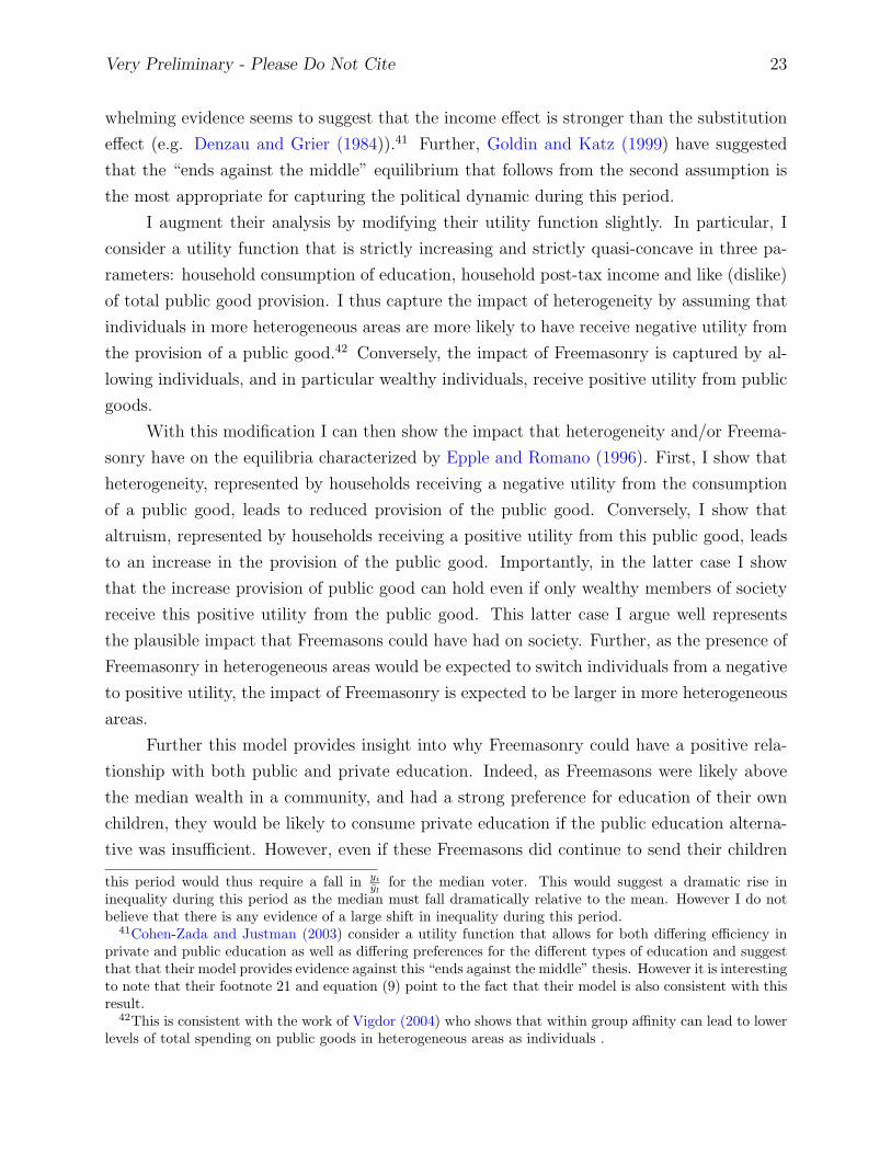
whelming evidence seems to suggest that the income effect is stronger than the substitution
effect (e.g. Denzau and Grier (1984)).41 Further, Goldin and Katz (1999) have suggested
that the “ends against the middle” equilibrium that follows from the second assumption is
the most appropriate for capturing the political dynamic during this period.
I augment their analysis by modifying their utility function slightly. In particular, I
consider a utility function that is strictly increasing and strictly quasi-concave in three pa-
rameters: household consumption of education, household post-tax income and like (dislike)
of total public good provision. I thus capture the impact of heterogeneity by assuming that
individuals in more heterogeneous areas are more likely to have receive negative utility from
the provision of a public good.42 Conversely, the impact of Freemasonry is captured by al-
lowing individuals, and in particular wealthy individuals, receive positive utility from public
goods.
With this modification I can then show the impact that heterogeneity and/or Freema-
sonry have on the equilibria characterized by Epple and Romano (1996). First, I show that
heterogeneity, represented by households receiving a negative utility from the consumption
of a public good, leads to reduced provision of the public good. Conversely, I show that
altruism, represented by households receiving a positive utility from this public good, leads
to an increase in the provision of the public good. Importantly, in the latter case I show
that the increase provision of public good can hold even if only wealthy members of society
receive this positive utility from the public good. This latter case I argue well represents
the plausible impact that Freemasons could have had on society. Further, as the presence of
Freemasonry in heterogeneous areas would be expected to switch individuals from a negative
to positive utility, the impact of Freemasonry is expected to be larger in more heterogeneous
areas.
Further this model provides insight into why Freemasonry could have a positive rela-
tionship with both public and private education. Indeed, as Freemasons were likely above
the median wealth in a community, and had a strong preference for education of their own
children, they would be likely to consume private education if the public education alterna-
tive was insufficient. However, even if these Freemasons did continue to send their children
this period would thus require a fall in yi
ylfor the median voter. This would suggest a dramatic rise in
inequality during this period as the median must fall dramatically relative to the mean. However I do notbelieve that there is any evidence of a large shift in inequality during this period.
41Cohen-Zada and Justman (2003) consider a utility function that allows for both differing efficiency inprivate and public education as well as differing preferences for the different types of education and suggestthat that their model provides evidence against this “ends against the middle” thesis. However it is interestingto note that their footnote 21 and equation (9) point to the fact that their model is also consistent with thisresult.
42This is consistent with the work of Vigdor (2004) who shows that within group affinity can lead to lowerlevels of total spending on public goods in heterogeneous areas as individuals .

Very Preliminary - Please Do Not Cite 24
to private schools, the positive utility that they received from the education of others would
still lead to higher provision of public education. Then as the quality of the public alter-
native gradually improved, with the increase in local taxation which would occur gradually
over time, more and more Freemasons would send their children to the public alternative.
In the first sub-section below I define the utility function of interest and characterize the
equilibria following Epple and Romano (1996). I also discuss the impact of my augmentation
on these equilibria. In the second sub-section I examine the plausible impact that an increase
in heterogeneity in a community will have on this equilibrium and in a final sub-section I
examine the impact that the presence of Freemasonry would have on this equilibrium. The
proofs are collected in Appendix A.
5.1 Utility Functions and Equilibrium
All households are assumed to have the same strictly increasing, strictly quasi-concave and
twice continuously differentiable utility function U(x, b, αE) over educational services, x, the
numeraire bundle, b, and the households benefit from the production of a public good, αE.
In this model, E is the production of the public good, education, by a community and α is
a scalar that may differ across households that measures that households benefit from the
good.
The final (third) term in this utility function is designed to capture the effects of both
heterogeneity and Freemasonry that I am trying to study with this model. A negative α can
be interpreted as an inherent dislike for public goods that are used by others. Thus, while a
household will gain utility from using the public good directly, if the household chooses to
consume the public good, the fact that others are consuming the public good that is being
at least partially funded by their taxes causes them disutility.
Conversely, a positive α represents an inherent appreciation for public goods. In par-
ticular it represents the fact that some people receive positive utility from the availability of
a public good. That there are many groups and individuals today with positive α is demon-
strated by the high level of philanthropy in the United States. The historical Freemason
literature indicates that Freemasons were likely to have a positive α, especially when the
public good of interest was public education.
I maintain the first two assumptions of Epple and Romano (1996), namely that:1. Educational services are a normal good, and
2. For x > 0, b > 0, x and b >> 0, U(x, b, ·) > U(0, b, ·) and U(x, b, ·) > U(x, b, ·).Following Epple and Romano (1996) there is diminishing marginal utility (DMU) in the
consumption of the numeraire good. Thus, if U(x1, b1, ·) = U(x2, b2, ·) and b2 > b1, then∂U(x1,b1,·)
∂b> ∂U(x2,b2,·)
∂b.

Very Preliminary - Please Do Not Cite 25
Individuals are allowed to consume private education, x, at a price p to maximize their
utility subject to the budget constraint y(1−τ) = px+b where y indicates household income,
τ is the prevailing tax rate in a community and the other terms are as previously defined.
Or they can consume public schooling for free. Households then maximize their utility by
choosing between consuming either private or public education by solving:
max{[
maxx
U(x, y(1− τ)− px, αE)], [U(E, y(1− τ), αE)]
}(1)
From the second assumption above, all households will consume some private education
if E = 0. Then, for some E > 0 households will switch to consuming the publicly provided
education. For a given level of taxation, E(·) defines the level of public education for which
a household is indifferent between consuming private education and public education. Thus,
for α = 0, which is equivalent to the case considered by Epple and Romano (1996), the utility
of the household will not be affected by changing levels of provision of the public good for
values of E < E(·). However, for E > E(·), utility will increase with the level of E as this
household is consuming the public education directly. This relationship is demonstrated in
Figure 5(a) which is identical to Figure 1 of Epple and Romano (1996) and the curvature
in the indifference curves to the right of the E(·) curve are the strict quasiconcavity of the
function.
As U(·, ·, ·) is strictly quasi-concave and strictly increasing in the third parameter, a
decrease in α will lead to a decrease in utility for all values of E, with the magnitude of
that decrease increasing with E. Additionally, the E(·) curve of a household will shift to
the left, analogous to a negative income shock, as I show in Lemma 2 (see Appendix A for
details). In Figure 5(b) I demonstrate the impact of a move from α = 0 to a negative α on
the indifference curves in (E, t) for a sample household. Conversely, an increase in α will
lead to an increase in utility for all values of E and cause a rightward shift of E(·) as shown
in Figure 5(c).
I now examine the impact that shifts in the utility function induced by a changing
α can have on equilibrium outcomes. As I will maintain the assumption that the price
elasticity of the implied demand for public education is larger than the income elasticity,
which leads to the “ends against the middle” result of Epple and Romano (1996), I will
focus on comparative statics of the equilibrium that they characterize in Proposition 3. I
will begin by presenting their result and then discuss how a change in α would effect the
equilibrium.
Though I discuss it in more detail in the appendix, it is essential to provide a definition
of the government budget constraint (GBC). Here the GBC is defined to be the educational

Very Preliminary - Please Do Not Cite 26
expenditure per household, E∗, for those attending school. Thus,
E∗ =tY
N(2)
where t is the taxation rate, Y is the total taxable income (wealth) of the community and N
is the number of households sending their children to school. Note that N will necessarily
be a function of t and E. Indeed from Figure C it is clear that households choose to send
their children to either public or private schools as a function of E and t.
Under the assumption concerning elasticities discussed above, in Proposition 3 Epple
and Romano (1996) show that any interior majority voting equilibrium, (E, t), satisfies and
requires the following four characteristics:1. There is a household with income yl that weakly prefers public consumption at point
(E, t) to all other points along the GBC
2. There is a household with income yh that is indifferent between public and private
consumption at point (E, t)
3. yl < yh
4. ρ =∫ yh
ylf(y)dy = 0.5
An example of this “ends against the middle” equilibrium is provided in Figure 6(a) which
reproduces Figure 7 from Epple and Romano (1996).
Though I defer a formal proof until Appendix A, in Figures 6(b) and 6(c) I provide
some intuition for how a change in α can lead to a change in the equilibrium. In these figures I
demonstrate how shifts in the utility functions of the two households that were the threshold
of the ‘rich-poor coalition’ can destabilize the previous equilibrium. A similar destabilization
would happen if an increase (decrease) in α shifted households across one of the thresholds.
Though it is not possible to demonstrate in a simple figure such as this, in the appendix
I show that an increase (decrease) in α that either shifted one of the threshold households
or shifted other households across the threshold would lead to an increase (decrease) in the
provision of public education.
5.2 Effect of Freemasonry
The historical literature suggests that Freemasons in the 19th century were altruistic in terms
of the provision of public education. Thus, individuals who were Freemasons were likely to
have a positive α in the model I describe above. While it is clear that an increase in α for
all individuals within a community would lead to an increase in public education, in this
sub-section I demonstrate how altruism among only an elite group, such as the Freemasons,
Very Preliminary - Please Do Not Cite 27
can induce higher public good provision in the “ends against the middle”-type equilibrium
discussed above.
My central result from this model is that an increase in altruism among wealthier
members of a community, in particular the voters above the median income and near the
upper threshold of the poor-rich coalition in the model specified above, leads to an increased
provision of the public good. The general intuition is that a change in the preferences of
individuals near this threshold is likely to either (1) shift the utility of the threshold household
to the right or (2) shift the utility of a household below the threshold to the right and past
the threshold. Lemma 1 presents this result and its proof is provided in Appendix A.
Lemma 1. Public good provision weakly increases with increased altruism among above-
median voters who are near the upper threshold of the rich-poor coalition. The probability of
a strictly positive increase in public good provision, as well as the magnitude of the change,
increases with both the size of the change in α as well as the number of voters affected by
this change.
As Freemasons tended to be above the median in terms of income, but not the wealth-
iest, it is likely that many of them were in the neighborhood of this upper threshold (see
Section ??). Thus, as men within a community became Freemasons and/or Freemasons near
this threshold migrated to a community, the increase altruism for public education that was
a central component of Freemasonry would lead to legislation for higher taxes and better
public good outcomes.
There are two important extensions to this result. First, while heterogeneity will lead
to lower public good provision, as it lowers the α for all types of individuals, Freemasonry
will have a larger impact in heterogeneous areas as Freemasonry will induce a switch from a
negative to positive α for this elite group. Second, as Freemasons tended to be very politically
active, it is possible that they could have used their influence to affect the perception of public
goods of other members of the community. In this case, the impact of Freemasonry will be
much stronger than that suggested by Lemma 1. Thus, though increased altruism among an
elite group is sufficient to explain changes in public good provision, the dramatic observed
impact of Freemasonry suggests that they were using their influence to influence voters.
The impact of this influence would be particularly significant in heterogeneous areas where
they could convince individuals across the income distribution to shift from a negative to a
positive α.

Very Preliminary - Please Do Not Cite 28
6 Data
6.1 Freemasonry Membership Data
American Freemasonry is a fully federated system with the lodges of each state reporting
solely to the Grand Lodge of that state. Each year, each of the Grand Lodges would hold
a state conference and representatives from each lodge were expected to attend this confer-
ence.43 After these conferences, the Grand Lodges would publish a volume, typically called
the Grand Lodge Proceedings of [name of state], which would report the discussions that
were held during the conference and correspondence with other Grand Lodges throughout
the United States and the world.
Beginning in 1850, these Grand Lodge Proceedings began to publish either lists of the
members of each lodge in the corresponding state or memberhsip statistics for each of these
lodges.44 While Grand Lodges could not form in a state until that state had officially entered
the Union, lodges would still form in those areas under the jurisdiction of one of the other
Grand Lodges.45 Thus, as census data is available for some areas before they become states
(e.g. Dakota Territory, Indian Territory, Nevada Territory, etc.), Freemason membership
data can also be constructed for many of these states from the Grand Lodge Proceedings of
other states.
Using the historical Proceedings from each of the Grand Lodges, I was thus able to
collect lodge level membership data for each state from 1850 to 1900. Though data is avail-
able for all states, I focus on the Western United States in this study. In particular I include
all states west of the Mississippi plus Illinois, Indiana and Wisconsin.46 The Western United
States provides a very interesting environment for studying the role of a social institution
such as the Freemasons on development, as much of this region was just beginning to develop
during this period. Further, this sample includes a variety of states at different stages of
development. In principle I would eventually like to include all the states in my study, but
time limitations have made this impossible for the current study.47
43The cost of transportation, lodging, etc. for these conferences would typically be subsidized by the homelodge.
44A few states have this membership data available before 1850: Rhode Island has data going back as faras 1790, Tennessee has data starting in 1820, Virginia starts in 1800, etc. However, all of the state havesome sort of membership data available by 1850.
45This is the mechanism which allowed for Freemasonry to spread as individuals were not allowed tospontaneously establish lodges. As an example, the early lodges in the state of California were under thejurisdiction of the states of Illinois and Missouri.
46I include these latter states for two reasons. First, is because these are the location of the second wave ofindustrialization in the United States, which began during the period in question, and I think it is importantto understand the role that Freemasonry may have played in this. Second, is because this is the area whereI grew up - I actually had one of the earliest Masonic orphan homes in my hometown.
47In theory I could just send these membership data to a company for digitization. In practice, idiosyn-

Very Preliminary - Please Do Not Cite 29
I collected this membership data decennially and county-level estimates of the number
of Freemasons were calculated by aggregating all Lodges within a county, as this allows me to
match this membership data to the most disaggregated socioeconomic data available during
this period from the US census (see below for more details on this data).48 Typically, most
of the Proceedings have a statistical abstract or appendix that lists at least the name of
the lodge, the number of the lodge and the number of Master Masons. In many cases these
appendices also contain the geographic location of the lodge, either city or county, in that
year. However, this geographic data is not available for all years in every state.
For this present study, lodge location was usually determined using the information
published in the 1900 Proceedings. However, for several states, the location of lodges that
became extinct before 1900 are not reported.49 For these extinct lodges, the location is
determined in two ways: First, when available, the location is extracted from one of the
previous Proceedings. Second, for lodges where this is not possible the location of the lodge
is sometimes imputed by matching the name of the lodge to cities in that state (lodges were
often named after the town where it was located or vice versa). This is not always possible
as the lodges often either take on Masonic names that do not match up to city names or the
same city name appears in more than one location in a state.
6.2 Share of Wealth Invested in Freemasonry
In this sub-section I describe my calculations of the share of wealth invested in Freemasonry.
The estimates of the investment in Freemasonry as well as total needed for these calculations
are described separately here.
6.2.1 Investment in Freemasonry
Lower bound estimates of the share of total wealth invested in Freemasonry are reported
in Figures 1 and 2. Figure 1 reports my estimate of the national aggregate and Figure 2
reports the means and standard deviates of county data for all states in my sample separately.
Here I discuss my approach for calculating this lower bound estimate and discuss why it is
appropriate to treat this as a lower bound.
Though there are a variety of approaches that I could have used to estimate this
quantity, I chose to calculate a lower bound estimate by comparing the total wealth in a
crasies in each publication of the Proceedings for each state makes this effectively impossible.48In principle, I actually have city/village level Freemason membership numbers available. However, these
data are not useful for the present study as there is no easily accessible, geographically comparable sourceof socioeconomic data for these cities.
49Several states continue to publish the location of extinct lodges in each revision of the Proceedings.

Very Preliminary - Please Do Not Cite 30
geographical area to an estimate of the total amount of money spent on initial membership
fees alone. Thus, my lower bound estimate of the total investment, IFLB, in Freemasonry is
simply
IFLB = (Membership Fee)× (# Masons)
and then I divide this quantity by the total wealth (discussed in the section ‘Total Wealth’
below). As data on the membership fees charged by individual lodges is unavailable, I used a
constant value of $50 across all states and periods in calculating this lower bound as discussed
immediately below.
In practice, membership fees varied significantly by state, and by lodge as the Grand
Lodge of each state only has the authority to set the minimum membership fee permitted.
Thus, though I was able to collect some data on minimum membership fees, which I provide in
Appendix C, the actual membership fees charged by individual lodges was often significantly
different. Further, the data that I do have on membership fees are from the late 19th century,
which are anecdotally less than fees charged earlier in the century. The value of $50 that I
have used was selected to be a rough average of the lodge membership fees during at least
the first 70 years of the 19th century, though fees likely varied from $30-200.
However, this estimate should be treated as a lower bound of the total investment in
Freemasonry for several reasons. First, many Masons joined one of the sister organizations
of Freemasonry, which all had additional initiation fees and annual fees. Two prominent
examples are the Knights Templar and the Royal Arch Masons. The the Knights Templar,
in which between 10-30% of Freemasons participated, cost an additional $75 in New York,
$100 in Chicago and $230 in San Francisco (Dumenil 1984, Hope 2005). And though the
fee and participation rate likely varied by state, Royal Arch Masonry in California had
initiation fees of $30 and accounted for nearly one-third of Freemasons in California.(Royal
Arch Masons of California 1882).50
Second, the variety of vestments that were required for Freemasonry and its various
suborders were often very expensive. Though I was unable to locate any reliable data on
the cost of clothing for the main organization, data on the cost of vestments for the Knights
Templar is available give an idea of how significant these costs might be. Before a mason
could become a Knights Templar, a uniform costing around $40-100, exclusive of the cost of
a horse, was required in addition to the initiation fee.51 Indeed, these uniforms were so costly
that the total value of uniforms worn in a single Templar parade was $1,000,000, which is
503,827 of the 12,132 Freemasons in 1880 were also Royal Arch Masons.51Hope (2005) reports that this uniform cost around $100 in California. An article in the Washington
Post provides a slightly lower estimate of $40 (The Wasington Post, September 27, 1889, pg. 1). Dumenil(1984) reports a cost of $71.

Very Preliminary - Please Do Not Cite 31
roughly equivalent to $100,000,000 in current dollars.52
Third, this figure does not include the number of women who were members of the
Eastern Star nor estimates of the investments that they may have made in that organization.
There were nearly 50,000 women in this organization in 1890, which was one-ninth of the
total men in Freemasonry during this time (Stillson and Hughan 1890).
In addition to these fixed costs, which I argue can be interpreted as an investment,
Freemasonry had a variety of non-trivial annual and more regular fees. Annual fees paid
to both the local and the state Grand Lodge were likely at least $5 in most states, which
was not an insignificant cost as the GDP per capita in many Western states was below $100
(Figure 3). And a variety of Freemason social events, such as balls and the like, would also
require further contributions from the Masons.
Further, charitable giving was typically a very important responsibility as evidenced
by their frequent discussion in various Grand Lodge Proceedings. The beneficiaries of these
charities varied but the most popular causes were for the support of widows or orphans
(through orphanages), educational funds or the support of sister lodges in the state or else-
where in the county in a time of crisis. These donations were typically a few dollars per
Mason per year, which was often a significant amount of money during this time. Indeed,
one Templar picnic in New York raised $10,000 (approximately $1 million in present dollars)
for one of their charitable funds.53
6.2.2 Estimates of Total Wealth
Here I discuss the estimates of total and county-level wealth that were used for calculating
the share of wealth invested in Freemasonry. Estimates of the total wealth in the United
States used for Figure 1 are drawn from Goldsmith (1952). However, the estimates of county
level wealth used in Figure 2 are my own and require some justification.
Though the total amount of wealth is not directly available in the historical U.S. cen-
suses, Goldsmith (1952) provides estimates of the total wealth in the United States for several
decades. His work, which draws on the work of Kuznets (1946) and others uses data avail-
able in the census to generate estimates of the total wealth. Though these estimates require
several assumptions, and in particular a relatively strong assumptions about the relationship
between value of farm real estate and agricultural capital, they are to my knowledge the best
available.54 As Goldsmith (1952) only provides estimates of the total wealth in the United
52The Wasington Post, September 27, 1889, pg. 1.53The New York Times, October 5, 1870, pg. 2).54Kuznets (1946) and Goldsmith (1952) generate an estimate of the total amount of agricultural capital in
land by multiplying the total value of farm real estate by one-fifth, which was the average of improvementsto real estate in 1900.
Very Preliminary - Please Do Not Cite 32
States for 1800, 1850, 1880, 1890 and 1900, estimates of the share of wealth invested in
Freemasonry is restricted to these years (Figure 1).
Estimates of total county-level wealth are not available for this period. However, there
are two estimates of capital available at the county-level in each wave of the census. The first
is an estimate of the physical capital in manufacturing: ‘Total capital invested (in dollars)
in manufacturing’ which includes capital invested in both buildings and machinery.55 The
second, ‘Present cash value of farming implements & machinery’, is an estimate of the
physical capital in agriculture. I use these two measures of capital to estimate the total
wealth in each county.
My approach to estimating county-level wealth is necessarily rough as these two vari-
ables only cover a fraction of the total wealth in a county. In particular, the national aggre-
gate of these two variables represents approximately one-sixth of the total wealth throughout
the second half of the 19th century.56 In lieu of a more precise way of estimating county-level
wealth, I use this “rule” of a ratio of 6:1 between total wealth and the amount of capital
represented by these two variables to derive rough estimates of total county-level wealth.
Thus, my estimate of the total wealth in a county is simply the sum of the agricultural
and manufacturing capital reported in the U.S. Census for that county scaled up by a factor
of 6.57 However, as the true relationship between total wealth and these measures of capital
is likely to vary by county, this is necessarily only a “back of the envelope” estimate.
Though this approach for estimating county-level wealth is thus quite rough, I believe
it is adequate as I use it only to provide an approximation of the magnitude of the investment
in Freemasonry. And though there are other possible approaches to estimating total wealth
at the county-level, these approaches will in general require very strong assumptions. In
particular, assessing the value of agricultural land is particularly difficult, though essential
for deriving precise estimates of county level wealth.58
6.3 Dependent Variables
The educational variables that are used in this analysis are drawn from two key sources. The
first, which are used primarily for the cross-sectional analysis, are county-level aggregates
available from the historical U.S. censuses. The second are the 1% IPUMS historical samples
55That it includes total capital in manufacturing is indicated by Kuznets (1946) who calculates the totalvalue of manufacturing buildings as a ratio of this amount.
56Goldsmith (1952) reports total wealth in the United States in 1900 at $55 billion while the aggregate ofthese two variables in the census data is $10.6 billion and the corresponding values for 1880 are $22.4 billionand $3.2 billion.
57I use the extracts from the historical U.S. Censuses developed by Michael Haines. ICPSR 2896.58Kris Mitchener, personal communication.

Very Preliminary - Please Do Not Cite 33
which are used for the panel estimates.
6.3.1 Census County Aggregates
The cross-sectional analysis focuses on three types of dependent variables that are available
in the historical U.S. censuses.59 The first type is school enrollment data which is available
for 1850, 1870, 1890 and then frequently throughout the 20th century. Second, in 1870 there
is data on the level of taxation at the local (town/city), county and state level. Finally,
which is only available for 1850, is a variety of detailed data concerning the structure of the
funding for private versus public school as well as the total number of teachers.
Though educational enrollment data is available in many of the censuses, it differs
slightly between each of the censuses. Here I discuss the type of enrollment data that is
available in 1850, 1870, 1890 and 1940. Though in some years it is possible to calculate en-
rollment separately by gender or by race, neither the Freemasonry historical record nor the
simple theoretical framework have any separate predictions about these quantities. Thus,
while I mention them here as they be of interest for future analysis, the focus of my quanti-
tative analysis of enrollment will focus on gross enrollment.
In 1850, the data on school enrollment is available in two forms. First it is possible to
separately identify the number of students in private and public schools using the following
two variables: ‘Number of pupils at academies and other schools’ and ‘Number of pupils in
public schools’. While this would be an interesting distinction to study, only 13 counties in
in my sample have any data on these academies, and it is thus impossible to study them
using data on only the Western United States. Second, it is possible to calculate the total
enrollment rate among whites, which will be the variable I will focus on below - though it
is possible to separately identify enrollment rates among (white) girls and boys using these
data.
For 1870, it is only possible to calculate the gross enrollment rate. I calculate this
gross enrollment rate by dividing the ‘Total persons in school’ by the total number of youth
ages 5-18. Though there is relatively extensive data on attendance among several different
groups (e.g. ‘native-born’, ‘foreign-born’, ‘colored’), the denominator - i.e. the total number
of youth of these different groups - is not available.
For 1890, it is possible to calculate school enrollment in three different ways. First,
it is possible to calculate the total enrollment rate in common schools among whites by
dividing the number of white men and women in common schools by the total native and
foreign whites youth.60 Second it is possible to separately calculate enrollment among white
59I use the extracts from the historical U.S. Censuses developed by Michael Haines. ICPSR 2896.60The data do not allow me to separately identify the number of foreign versus native whites enrolled as

Very Preliminary - Please Do Not Cite 34
men and white women. Finally, it is also possible to calculate the total enrollment among
‘colored’ youth during this period.
For 1940, it is possible to separately measure the enrollment rates among youth of
elementary school, lower secondary, upper secondary and college age separately. Similar
data is available from 1910-1930 though I do not include it in this analysis as the results are
generally quite similar - and in the few cases where there are differences I mention them.
In 1870, there is data on the total amount of state, county and local taxes paid by the
residents of each county. While it is unclear how local taxes are being used, and it is likely
to differ across counties, the public good aspect of Freemasonry predicts that the ratio of
local to state should be higher in counties with more Freemasons.
Though the number of states with both economic and Freemason data is rather limited
for 1850, the data on education is the most extensive in 1850 along two important dimensions.
First of all, the amount of income for public schools, private schools and colleges from a
variety of sources - including taxation and public funds - is available. Second, in 1850 there
is data on the total number of teachers in public schools, private schools and colleges so that
it is possible to calculate the teacher to pupil as well as the teacher to total youth population
ratio.
6.3.2 IPUMS 1% Sample
While the county-level aggregates provide data on the universe of children in calculating
enrollment rates, the definition of child enrollment is not constant throughout the 19th
century and is thus not appropriate for panel data estimation approaches. However, IPUMS-
USA has made available 1% samples from each of the 19th century censuses that allow for
the creation of a child enrollment panel (Ruggles, Alexander, Genadek, Goeken, Schroeder,
and Sobek 2010).
These data are used to construct a panel of county-level youth enrollment among
children ages 5-18 decennially for 1850-1900. Though these data are more sensitive to mea-
surement error as it is only a 1% sample, the panel structure allowed by this data provides
an important tool for verifying the robustness of my cross-sectional results.
6.4 Demographic and Economic Data
Throughout my analysis I include a variety of demographic and economic variables that are
drawn from the historical US censuses. The meaning of many of these variables is quite
clear. Indeed, the total size of the population, the number of men, the number of people
in this case I lack the appropriate numerator.
Very Preliminary - Please Do Not Cite 35
living in cities of different sizes, etc. are standard census quantities. However, throughout
this analysis I include four separate measures of the income and wealth of these counties. I
feel that a short discussion for including these quantities separately is warranted.
Two separate measures of wealth are available throughout the census data of the late
19th century. The first of these is the ‘amount of capital invested in manufacturing estab-
lishments’, which I call KM . The second is the ‘value of farming implements & machinery’,
which I call KA. It would be inappropriate to aggregate these measures together for the
estimation as each of these variables only measure a fraction of the total capital in a county
and this fraction is unlikely to be the same across the two sectors. However, as long as the
ratio between the measured amount of capital and the true amount of capital in each sector
is constant across a state, and I include both in my regression, then state fixed effects will
capture this ratio.
The data on income is slightly more limited than that of wealth.61 In particular, while
data on manufacturing output - the ‘value of annual product in manufacturing establish-
ments’ - is available beginning in 1850, there is no aggregated data on agricultural output
available until 1870 (‘total (estimated) value of all farm productions, including betterments
& addition to stock’). In practice, it is possible to extend the approach of Tucker (1843),
Seaman (1868) and Easterlin (1960) to county level data and simply multiply the agricultural
production of each county by the corresponding prices (available in the two first references).
However, after having done this for one state I decided that the effort involved - as all the
agricultural production data needs to be hand entered due to the low quality of the avail-
able scanned agricultural censuses - was significantly less than marginal benefit of having a
measure of agricultural output for these earlier years.
A possible concern is that the fraction of the real wealth or income that is measured by
these variables may vary with the some of the either right-hand side variables, such as the
number of Freemasons or the total population. This type of measurement error would lead
to biased point estimates. Unfortunately, I have been unable to identify any sources that
discuss in detail the collection of these variables or possible concerns with using them.62
61Estimates of both forest production are available beginning in 1870 and estimates of mining productionare available beginning in 1880. However, this data would also need to be hand entered as it is not availablein any digital form that I know of. This omission is unlikely to have a large negative impact on my results.
62I did on several occasions contact the US Census Office. While they were very helpful, there did notseem to be very much institutional knowledge about the specific of the collection of these variables. Andreturning to the old census reports did not reveal very much information.

Very Preliminary - Please Do Not Cite 36
6.5 Shifting County Borders
County definitions in many states changed significantly during the second half of the twenti-
eth century. Thus, as my lodge location data is primarily from 1900, I needed to account for
the possibility that a lodge was actually in a different county in an earlier year. In particular,
I needed to find the relationship between counties in 1900 and each of the other years for
which I have Freemason data: 1850, 1860, 1870, 1880 and 1890.
My approach for addressing this problem proceeded in two steps. First, historical GIS
maps of county borders in the United States were obtained from the National Historical
Geographical Information System.63 I then used the GIS ArcMap software to find counties
were border definitions likely occurred by comparing the 1900 county map with the county
maps for each of the years. In each case, I calculated the intersection of two county maps,
using a one-mile tolerance, which would identify any changes in county definitions that were
more than one mile.
In the second step, in order to correct for mistakes in this matching process, I checked
all the likely matches found in ArcMap by hand. In particular there are many cases where
county borders between the two county maps would shift by three or four miles. Or in some
cases there were changes where a frontier county would ‘lose’ much of its frontier territory -
though it is unlikely that this there was any significant population in this frontier territory in
earlier years. This second step was thus subjective and relied a bit on my ‘best judgement’.
But it was essential, as there were many ‘mistakes’ in the first matching step. Also, it was
done entirely before any economic analysis was done so it is unlikely to affect the results.
6.6 Potential IVs
While there are a variety of variables available in the census that one might think would be
appropriate, in all cases these variables have either an implausible first stage or exclusion
restriction. As examples I will show how three leading possibilities are not appropriate: (1)
Share Catholic [strong first stage, implausible exclusion restriction]: strong and significant
first stage as the Freemasons and Catholicism had an antagonistic relationship during this
period, but the Catholic Church also had an independent impact on public education as
they were actively promoting and trying to secure funding for private, religious schools.
(2) Share Foreign [no first stage]: there is no evidence that foreigners received preferential
treatment or were excluded from the Freemasons. (3) Blue Laws [no first stage]: While
some lodges were completely dry and encouraged alcohol abstinence among their members,
members of other lodges would gather together after meetings to drink together - and this
63http://www.nhgis.org/

Very Preliminary - Please Do Not Cite 37
type of variation is found within states as well as across. Similar argument can be applied
for every other variable in the US census as well as other variables that would require great
expense to collect.
7 The Impact of Freemasonry on Educational Enroll-
ment
Here I use the county-level data on educational enrollment available in the US census to
estimate the impact of Freemasonry on education. The analysis is divided into two major
sub-sections. The first uses cross-sectional data to examine the impact of Freemasonry on
education during two historical periods: (1) the late 19th century and (2) the early- to mid-
20th century. Then, in a second sub-section, I use a panel of education and Freemasonry
data to verify the robustness of these results to the possibility of unobserved heterogeneity,
endogeneity and autocorrelation.
Throughout this analysis, I will focus on estimation of a very simple relationship be-
tween educational enrollment and a variety of socioeconomic variables. In particular, I will
model the educational enrollment in a county as
yi = X ′iβ + εi (3)
where i indexes counties, yi is the educational enrollment in county i, Xi contains a variety
of socioeconomic variables and εi is the error process. This simple parameterization is based
on the model used by Goldin and Katz (1999) in their examination of county-level data from
Iowa in 1915 though I augment the set of socioeconomic variables to include my measure
of Freemasonry, the number of Freemasons per capita. Also, my dependent variable differs
slightly. While they focus on high school and college enrollment, which is only available
in later years, I focus on total enrollment among youth ages 5-18. I also include several
additional measures of wealth that are only available in early census data as well as the
percentage of the population that is male and over age 21. As only adult (21+) males
are eligible to becomes Masons, including this latter control ensures that my measure of
Freemasons is not just functioning as a proxy for adult males who are more likely to be
economically active than other segments of the population.
All analysis done here is at the county-level and all regressions include state fixed ef-
fects.64 While it is plausible that Freemasonry also had an effect on state level education
64In the case of the fixed effects panel data estimates, there are no state fixed effects as it is not possibleto identify the effect of variables that are time constant.

Very Preliminary - Please Do Not Cite 38
policies as suggested by the historical literature on Texas, most of the funding for educa-
tion was done at the local level as discussed above. Further, it would be very difficult to
measure the influence of Freemasons in explaining state-level differences as Freemasons were
ubiquitous in state, as well as national, politics.
7.1 Cross-Sectional Estimates
In this first sub-section, I use cross-sectional data to explore the the potentially changing
relationship between Freemasonry and educational enrollment during the early years of the
development of the American West. I begin this analysis by examining the relationship
between Freemasonry and total youth educational enrollment in 1870 and 1890. By 1870,
Freemasonry’s presence was already well established in the Western United States and the
organization continued to expand rapidly through 1890. Here, I find a strong positive rela-
tionship between Freemasonry and education. And this impact seems to be similar in both
agricultural and manufacturing communities.
In order to test for the possible lasting impact of this social institution, I then look at
the relationship between nineteenth century Freemasonry and enrollment rates in the early
and mid-twentieth century. As it is possible to separately identify primary, secondary and
tertiary educational enrollment in the twentieth century census data, I am able to examine
both the potential lasting impact of Freemasonry on primary educational systems as well as
the role that Freemasonry played in the second wave of educational expansion in the United
States. While there does not seem to be a significant lasting impact on primary education,
which is likely explained by the near universal primary education at this point, I do find
evidence of an impact on secondary and tertiary education. This effect seems to be most
pronounced among potential upper secondary students.
7.1.1 Education in the Late 19th Century
Between 1850 and 1870, Freemasonry spread very rapidly in the West and into the Midwest,
and by 1890 the organization was present in almost every county of the Western United
States. Here I examine the contemporaneous relationship between Freemasonry and educa-
tion during this period which I believe to be the height of Freemasonry influence. As both
measures of social homogeneity used by Goldin and Katz are available for this period, I
will be able to directly compare the ‘homogeneity effect’ observed by these authors to the
potential Freemasonry effect.
Table 1 presents the results from my analysis using the education, socioeconomic and
Freemason data from 1870 and 1890. For 1870 the dependent variable is the attendance

Very Preliminary - Please Do Not Cite 39
rate of youth ages 5-18; and in 1890 the dependent variable is the attendance rate among
all white children ages 5-20. In Columns (1) and (6), I reproduce the analysis of Goldin and
Katz (1999) and find somewhat similar results as these authors using my data. In particular,
in the 1870 data I find that measures of wealth as well as one of Goldin and Katz’ proxies
for social capital - social homogeneity as measured by the proportion of the population of
native heritage - have a significant positive effect on educational outcomes. Interestingly, in
the 1890 data, this same measure of social capital has a strong positive impact while their
other proxy for social capital, the share of the population in small towns, has a large negative
impact. This unusual result for their second social capital proxy could be driven by the fact
that my measure of town “smallness” is much larger than theirs - however, the reversal of
the sign with a significant point estimate is a peculiar result.65
In columns (2) and (7) I augment these regressions to include the per capita concentra-
tion of Freemasons. In both the 1870 and 1890 data I find that the number of Freemasons
per capita has a large and very significant impact on enrollment outcomes. Interestingly it
seems that the introduction of Freemasons per capita has only a weak effect on the point
estimates for Goldin and Katz’ proxies for social capital, suggesting that Freemasons are not
simply a measure of social homogeneity.
In the data from 1890, the impact of Freemasonry on education is of roughly the same
magnitude as that of social homogeneity. Indeed, while the estimated coefficient on Freema-
sonry is about thirty times larger than that for social homogeneity, the standard deviation
of the social homogeneity variable is about thirty times the size of that for Freemasons per
capita. However, in 1870 the total impact of Freemasonry is about twice that of social ho-
mogeneity as the coefficent is still thirty times larger while the standard deviation is only
one-fifteenth that of the measure of social homogeneity.
In columns (3)-(5) and (8)-(10) I disaggregate the counties by the type of economic
activity, in order to explore where the impact of Freemasonry was the strongest, if anywhere
in particular. To do this, I create three groups of activity: The first group, which I have
designed to be the ‘mostly agricultural’ counties are counties where the share of output from
manufacturing is at most one-third, are in columns (3) and (8). The second group is the
‘mixed’ group and is counties where the share from manufacturing is between one-third and
two-thirds. The final group is the ‘mostly manufacturing’ counties where the manufacturing
share is at least two-thirds.
As areas that are primarily agricultural have the the least dense populations, and
are thus more likely to have difficulty in providing common goods, it is unsurprising that
65Twentieth century data allows a much finer disaggregation of population. And in particular, theseauthors observe the share of the population in towns smaller than 1,700 persons, 1,700-2,500 persons, etc.
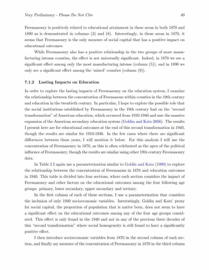
Very Preliminary - Please Do Not Cite 40
Freemasonry is positively related to educational attainment in these areas in both 1870 and
1890 as is demonstrated in columns (3) and (8). Interestingly, in these areas in 1870, it
seems that Freemasonry is the only measure of social capital that has a positive impact on
educational outcomes.
While Freemasonry also has a positive relationship in the two groups of more manu-
facturing intense counties, the effect is not universally significant. Indeed, in 1870 we see a
significant effect among only the most manufacturing intense (column (5)), and in 1890 we
only see a significant effect among the ‘mixed’ counties (column (9)).
7.1.2 Lasting Impacts on Education
In order to explore the lasting impacts of Freemasonry on the education system, I examine
the relationship between the concentration of Freemasons within counties in the 19th century
and education in the twentieth century. In particular, I hope to explore the possible role that
the social institutions established by Freemasonry in the 19th century had on the “second
transformation” of American education, which occurred from 1910-1940 and saw the massive
expansion of the American secondary education system (Goldin and Katz 2008). The results
I present here are for educational outcomes at the end of this second transformation in 1940,
though the results are similar for 1910-1930. In the few cases where there are significant
differences between these years, I will mention it below. For this analysis I will use the
concentration of Freemasonry in 1870, as this is often celebrated as the apex of the political
influence of Freemasonry, though the results are similar using other 19th century Freemasonry
data.
In Table 2 I again use a parameterization similar to Goldin and Katz (1999) to explore
the relationship between the concentration of Freemasons in 1870 and education outcomes
in 1940. This table is divided into four sections, where each section considers the impact of
Freemasonry and other factors on the educational outcomes among the four following age
groups: primary, lower secondary, upper secondary and tertiary.
In the first column of each of these sections, I use a parameterization that considers
the inclusion of only 1940 socioeconomic variables. Interestingly, Goldin and Katz’ proxy
for social capital, the proportion of population that is native born, does not seem to have
a significant effect on the educational outcomes among any of the four age groups consid-
ered. This effect is only found in the 1940 and not in any of the previous three decades of
this “second transformation” where social homogeneity is still found to have a significantly
positive effect.
I then introduce socioeconomic variables from 1870 in the second column of each sec-
tion, and finally my measure of the concentration of Freemasonry in 1870 in the third column

Very Preliminary - Please Do Not Cite 41
of each section. While Freemasonry has only a weakly positive effect on primary education,
there is a strong positive impact on all other levels of education. Here, however, the ef-
fect of Freemasonry is slightly weaker than social homogeneity as the ratio of the standard
deviations of social homogeneity and Freemasonry is about fifteen-to-one.
7.2 Panel Data Estimates
The above analysis focused on the estimation of equation (3) using cross-sectional data.
However, consistent estimation of equation (3) requires that Xi and εi are uncorrelated,
i.e. Cov(Xi, εi) = 0. However, this is unlikely to be the case as there are unobservable
characteristics of these counties that are likely to affect education, Freemasonry membership
and some, if not all, of the other socioeconomic variables contained in Xi. In particular, it
is likely that
yi = X ′iβ + ci + εi (4)
is a more accurate representation of the process determining yi, where ci represents unobserv-
able county-specific characteristics, and that Cov(Xi, ci) 6= 0. In this case, the cross-sectional
estimates presented in the previous section are inconsistent. Indeed, consistent estimation
of β using cross-sectional data would require the availability of either a suitable proxy or a
plausible instrument for ci, neither of which are clearly available (Wooldridge 2002).
However, using the 1% IPUMS data available for each decade from 1850 to 1900 to
estimate educational enrollment, I construct a county-level panel data set which allows con-
sistent estimation of (4).66 In particular, this panel data allows me to estimate
yit = X ′itβ + ci + εit (5)
where i indexes counties, t indexes decades and ci is the unobservable county effect. In this
simple panel data model, consistent estimates of β are available directly if Xit are strictly
exogenous conditional on ci, or E[εit|Xit, ci] = 0.
I estimate (5) using three different panel data sets of educational enrollment. The
first of these data sets has the most coverage in terms of time, spanning from 1850-1900,
but contains the least geographic coverage as it uses the earliest available county definitions
which tend to be more aggregated than later counties (T = 6, N = 451). The third data set
covers the fewest years, only 1870-1900, but offers the greatest geographical variation (T =
66IPUMS data is not currently available for 1890. For 1890 I impute educational enrollment using theICPSR 2896 data for this year as discussed above. A discussion of the implications of this imputation forthe reliability of my results is discussed below.

Very Preliminary - Please Do Not Cite 42
4, N = 1034) while the second, which covers 1860-1900, is a balance between geographical
variation and years covered (T = 5, N = 843).
In order to check the reliability of these different data, I first ignore the unobservable
county effects and replicate the cross-sectional analysis done above by calculating simple
OLS estimates using the pooled data. The results from this OLS are presented in column
(1) of Tables 3-5 and are very similar to the cross-sectional results, suggesting that the use
of the IPUMS data to impute the missing years of education will likely produce reliable
results.67 Further, as the results are largely similar across the three different possible panel
data sets, these results suggest that estimation using these different panels should produce
similar results throughout this analysis.
Second, I estimate equation (5) using the fixed effects panel data estimator, which
allows for arbitrary correlation between the unobservable county effect and the other ex-
planatory variables.68 These estimates, which are presented in the second column of Tables
3-5, provide weak evidence that Freemasonry had a positive impact on the development of
education as the estimates using both of the longer panels remain positive, with one estimate
significant at the 5% level. However, the estimated effect using the shorter panel with the
larger geographical coverage returns a point estimate that is effectively zero.
The difference between the point estimates from OLS and FE analysis may be at-
tributable to a variety of causes, which I will address in the following sections. First, it may
be the case that the Freemasonry variable is endogenous, in which case the first-differencing
of the FE estimator will exacerbate the bias due to this endogeneity. Second, it is likely that
educational enrollment is autoregressive as the availability of schools and teachers is likely
to be correlated over time. In this latter case the strict exogeneity condition is violated and
the estimates of (5) will be inconsistent. As this inconsistency is particularly severe for small
T, this could explain the unusual results obtained above using the short panel Wooldridge
(2002).
A major concern with the estimation of (3) and (5) is that there may be correla-
tion between Xit and εit due to the omission of a variable that affects both Xit and Yit.
For Freemasonry, in particular, this may be a significant concern as the presence of strong
community leaders is likely to affect the presence of Freemasonry and schools.
In the presence of this endogeneity, estimates of both equation (3) and (5) will be
67Estimates using only the IPUMS data for educational enrollment delivers similar results in general. Asan example, if I calculate the pooled OLS estimate using only the IMPUS data available for 1860, 1870,1880 and 1900, the magnitude, sign and significance of all but one the estimates remains the same (theonly exception is the urban variable which changes signs - though it is effectively zero in both cases). Oneimportant exception to this apparent reliability of the IMPUS data is the data available for 1850 which seemsto produce unreliable results.
68This is essential as it is likely that Cov[Xit, ci] 6= 0 for most, if not all, of the covariates in Xit.

Very Preliminary - Please Do Not Cite 43
biased. For (3) this bias is given by
β =Cov(Xit, βXit + εit)
V ar(Xit)
= β +σX,εσ2X
(6)
and for (5), since estimation is done by taking first differences and then using OLS, this bias
is given as
β =Cov(∆Xit, β∆Xit + ∆εit)
V ar(∆Xit)
= β +Cov(Xit −Xi,t−1, εit − εi,t−1)
V ar(Xit −Xi,t−1)
= β +σX,ε
σ2X(1− ρX)
(7)
where σX,ε is the covariance between Xit and εit, σ2X is the variance of Xit and ρX is the
correlation of Xit and Xi,t−1, all of which are assumed to be constant over time.
Correcting for the bias presented in equation (7) is possible if some other variable Zit
is available to be used as in instrument, e.g. Cov(∆Zit,∆Xit) 6= 0 and Cov(∆Zit,∆εit) = 0.
Though no appropriate instrument is evident, as was also the case with the cross-sectional
estimates presented above, the panel structure of the data allows us to study the bias is
encountered in estimation of equation (5).
In particular, Anderson and Hsiao (1982) and Arellano and Bond (1991) propose using
lagged levels (or differences) of the explanatory variables as instruments for estimation similar
to this. In the case presented here, using a explanatory variable that was lagged two periods
would indeed satisfy the exclusion restriction since Cov(Xi,t−2, εi,t−1) = 0. However, forXi,t−2
to be a good instrument, there must be a strong relationship between Cov(Xi,t−2,∆Xi,t). In
my case, it is unlikely that there is a strong relationship between the level of Freemasonry
in one decade and the change between two subsequent decades, especially since I am con-
ditioning on a variety of socioeconomic variables. As a weak instrument, Xi,t−2 is likely to
perform badly in practice.
Instead of instrumenting using Xi,t−2, I propose to estimate equation (5) using Xi,t−1.
The first stage of this IV approach is guaranteed to be meaningful, and while the estimator
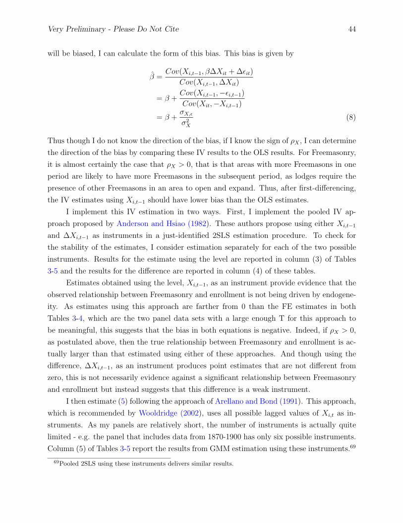
Very Preliminary - Please Do Not Cite 44
will be biased, I can calculate the form of this bias. This bias is given by
β =Cov(Xi,t−1, β∆Xit + ∆εit)
Cov(Xi,t−1,∆Xit)
= β +Cov(Xi,t−1,−εi,t−1)
Cov(Xit,−Xi,t−1)
= β +σX,εσ2X
(8)
Thus though I do not know the direction of the bias, if I know the sign of ρX , I can determine
the direction of the bias by comparing these IV results to the OLS results. For Freemasonry,
it is almost certainly the case that ρX > 0, that is that areas with more Freemasons in one
period are likely to have more Freemasons in the subsequent period, as lodges require the
presence of other Freemasons in an area to open and expand. Thus, after first-differencing,
the IV estimates using Xi,t−1 should have lower bias than the OLS estimates.
I implement this IV estimation in two ways. First, I implement the pooled IV ap-
proach proposed by Anderson and Hsiao (1982). These authors propose using either Xi,t−1
and ∆Xi,t−1 as instruments in a just-identified 2SLS estimation procedure. To check for
the stability of the estimates, I consider estimation separately for each of the two possible
instruments. Results for the estimate using the level are reported in column (3) of Tables
3-5 and the results for the difference are reported in column (4) of these tables.
Estimates obtained using the level, Xi,t−1, as an instrument provide evidence that the
observed relationship between Freemasonry and enrollment is not being driven by endogene-
ity. As estimates using this approach are farther from 0 than the FE estimates in both
Tables 3-4, which are the two panel data sets with a large enough T for this approach to
be meaningful, this suggests that the bias in both equations is negative. Indeed, if ρX > 0,
as postulated above, then the true relationship between Freemasonry and enrollment is ac-
tually larger than that estimated using either of these approaches. And though using the
difference, ∆Xi,t−1, as an instrument produces point estimates that are not different from
zero, this is not necessarily evidence against a significant relationship between Freemasonry
and enrollment but instead suggests that this difference is a weak instrument.
I then estimate (5) following the approach of Arellano and Bond (1991). This approach,
which is recommended by Wooldridge (2002), uses all possible lagged values of Xi,t as in-
struments. As my panels are relatively short, the number of instruments is actually quite
limited - e.g. the panel that includes data from 1870-1900 has only six possible instruments.
Column (5) of Tables 3-5 report the results from GMM estimation using these instruments.69
69Pooled 2SLS using these instruments delivers similar results.
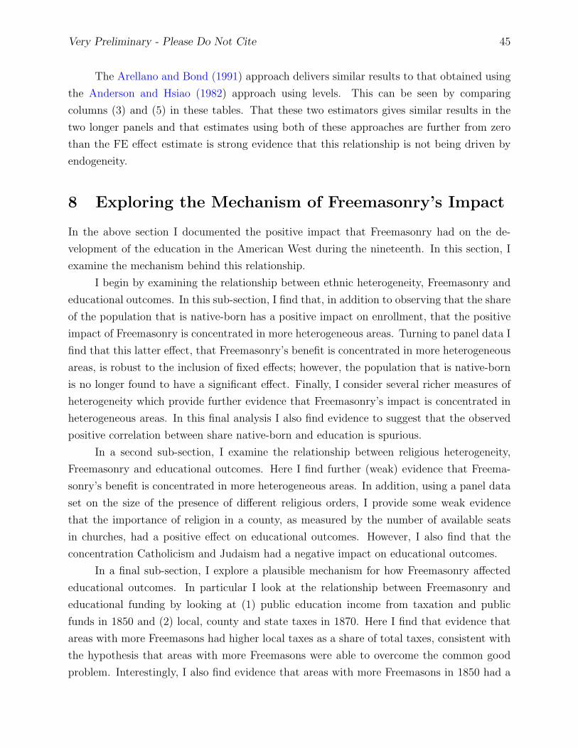
Very Preliminary - Please Do Not Cite 45
The Arellano and Bond (1991) approach delivers similar results to that obtained using
the Anderson and Hsiao (1982) approach using levels. This can be seen by comparing
columns (3) and (5) in these tables. That these two estimators gives similar results in the
two longer panels and that estimates using both of these approaches are further from zero
than the FE effect estimate is strong evidence that this relationship is not being driven by
endogeneity.
8 Exploring the Mechanism of Freemasonry’s Impact
In the above section I documented the positive impact that Freemasonry had on the de-
velopment of the education in the American West during the nineteenth. In this section, I
examine the mechanism behind this relationship.
I begin by examining the relationship between ethnic heterogeneity, Freemasonry and
educational outcomes. In this sub-section, I find that, in addition to observing that the share
of the population that is native-born has a positive impact on enrollment, that the positive
impact of Freemasonry is concentrated in more heterogeneous areas. Turning to panel data I
find that this latter effect, that Freemasonry’s benefit is concentrated in more heterogeneous
areas, is robust to the inclusion of fixed effects; however, the population that is native-born
is no longer found to have a significant effect. Finally, I consider several richer measures of
heterogeneity which provide further evidence that Freemasonry’s impact is concentrated in
heterogeneous areas. In this final analysis I also find evidence to suggest that the observed
positive correlation between share native-born and education is spurious.
In a second sub-section, I examine the relationship between religious heterogeneity,
Freemasonry and educational outcomes. Here I find further (weak) evidence that Freema-
sonry’s benefit is concentrated in more heterogeneous areas. In addition, using a panel data
set on the size of the presence of different religious orders, I provide some weak evidence
that the importance of religion in a county, as measured by the number of available seats
in churches, had a positive effect on educational outcomes. However, I also find that the
concentration Catholicism and Judaism had a negative impact on educational outcomes.
In a final sub-section, I explore a plausible mechanism for how Freemasonry affected
educational outcomes. In particular I look at the relationship between Freemasonry and
educational funding by looking at (1) public education income from taxation and public
funds in 1850 and (2) local, county and state taxes in 1870. Here I find that evidence that
areas with more Freemasons had higher local taxes as a share of total taxes, consistent with
the hypothesis that areas with more Freemasons were able to overcome the common good
problem. Interestingly, I also find evidence that areas with more Freemasons in 1850 had a

Very Preliminary - Please Do Not Cite 46
higher share of teachers per student in private schools. This suggests that Freemasons have
a stronger preference for education than other citizens. While my capture does not capture
this level of heterogeneity, it is consistent with my claim that Freemasons valued education
more than others.
8.1 Freemasonry and Ethnic Heterogeneity
The work of Goldin and Katz highlighted the negative relationship between ethnic hetero-
geneity and educational development in American history. Interestingly, while I consistently
find a positive relationship between educational enrollment and the share of a population
that is of native parentage, which supports the claim of these authors, this result does not
seem to be robust to the inclusion of fixed effects. Indeed, while in Table 5 I show that
this measure of homogeneity loses its statistical significance when controlling for unobserved
heterogeneity, estimation using panel data that spans from 1860 to 1900 produce significants
negative estimates of the relationship between homogeneity and educational outcomes as
shown in Table 4.
In this sub-section, I examine both this empirical phenomenon as well as the relation-
ship between Freemasonry and ethnic heterogeneity. As Freemasonry similarly shows (see
Section 9.2) a strong positive relationship with ethnic homogeneity, as measured by the share
of the population of native parentage, in pooled OLS regressions and a negative relation-
ship in fixed effects panel analysis, this suggests that the impact of Freemasonry and ethnic
homogeneity/heterogeneity may be related. And as Freemasonry encouraged the expansion
of public education by bringing men of all types together in support of a common cause, I
might expect that the Freemasonry effect would be more pronounced in more heterogeneous
areas.
My analytical strategy for looking at the relationship between Freemasonry, ethnic
heterogeneity and educational outcomes is very straightforward. In particular, I simply aug-
ment my previous analysis of educational enrollment to include an interaction term between
Freemasons per capita and the share of the population of native parentage. In Table 6, where
I report the results using the cross-sectional data available for 1870, I find that this interac-
tion term has a very significant negative coefficient. As areas that have a larger value of “%
native” are more homogenous, this coefficient indicates that the impact of Freemasonry on
education is attenuated in areas that are more socially homogenous. Indeed, the impact of
Freemasonry is four-fold greater in a community with no individuals of native parentage as
compared to a community that is 100% native.
Table 7 reports the results from this analysis using the 1860-1900 and 1870-1900 panel

Very Preliminary - Please Do Not Cite 47
data sets that contain data on the share of the population of native parentage. Note that
here, unlike before, I do not include the results that correct for endogeneity as the results
do not change substantively.
The central result of this table is that Freemasonry’s impact on education seems to be
the largest, by far, in areas that are the most heterogeneous. Indeed, in areas that are very
homogenous - e.g. the share of the population of native parentage is close to 1 - the impact
of the number of Freemasons on educational outcomes is estimated to be quite small.70
However, in areas that are very heterogeneous, an increase in the number of Freemasons is
predicted in a county is expected to have a very strong impact on education: if the number
of Freemasons per capita increased by 0.01 - e.g. one additional Freemason for each one
hundred local residents - in an area where 50% of the population was of native parentage,
this would lead to a 6-7% point increase in the educational enrollment rate. Perhaps most
interestingly is that this result is one of the few empirical results that is strongly significant,
with the same sign, across both data sets and specifications.
One potential concern with this analysis is that the measure of homogeneity used thus
far, the share of the population of native birth, does not truly reflect the homogeneity of a
community. Indeed, it is possible that a community with few individuals of native birth can
actually be quite homogenous. Thus, a second possible interpretation of the result for this
interaction term is that the Freemasonry effect is concentrated in areas with a large number
of recent immigrants.
In order to explore this issue, I restrict my analysis to 1870, 1890 and 1900 which allows
me to augment my analysis in two ways. First, I can divide the population native born into
the population native born of native parentage and the population native born of foreign
parentage. Second I can construct a measure of the ethnic fractionalization of an area. This
measure, which I call the ethnic fractionalization index (EFI), is constructed as
EFI = 1−n∑i=1
PiTotal Population
(9)
where Pi is the population in group i and i indexes the different ethnic groups distinguishable
in the census. While these censuses allow me to identify the origin of birth of foreign born
individuals, in practice this only accounts for 15% of the total individuals included in my
data. Thus, much of the variation in EFI is driven by the ratio of the number of native born
individuals with native-born parents as compared to those with foreign-born parents. The
data section above has more details on this measure.
70This is calculated by multiplying the coefficient for the interaction term times 1 - or close to 1 - andadding this to the coefficient for the Freemason term by itself.

Very Preliminary - Please Do Not Cite 48
Table 8 reports the analysis using these two more disaggregated measures of ethnic
homogeneity. Columns (1)-(7) provide estimates using pooled OLS and columns (8)-(14)
provide the fixed effects panel estimation results.71 Analysis examining the two measures of
parent nativity and EFI are done separately as these variables are closely related and it is
difficult to separately identify the impact of each.
In comparing column (1), which repeats the analysis used above, with column (2),
which disaggregates the share native by type of parentage, an interesting phenomenon
emerges: the strong positive relationship between nativity and educational outcomes dis-
appears. This is verified by columns (8) and (9) which report the same results controlling
for unobserved county-level heterogeneity. This suggests that the observed positive relation-
ship between nativity and educational outcomes is perhaps spurious.
In columns (3) and (10) I include my Freemasonry variable. Similar to the analysis
above using 1870-1900 data in Table 7 I find a significantly positive point estimate for
the pooled OLS and no effect for the fixed effects estimation. However, when I augment
this analysis to include an interaction term between Freemasonry and the two measures of
homogeneity, in columns (4) and (11) I find a positive, large and significant coefficient for
Freemasonry.
Interestingly, the estimated coefficient on both of the interaction term is negative,
which is the same as I found for the aggregate share of native-born in Table 7. Thus, while
it does not seem that nativity effects educational outcomes directly, it is the case that the
benefit of Freemasonry is concentrated in areas that are more heterogeneous.
Columns (5) and (12) consider the impact of my ethnic fractionalization index (EFI) on
educational outcomes. The effect of EFI is surprisingly weak, as an area with an EFI of one
- where every individual would from a different county - is expected to have an enrollment
rate that is only four points lower. However, the inclusion of an interaction term with
Freemasonry leads to much larger and significant estimates of its impacts. In particular,
it seems that this ethnic heterogeneity has a positive impact on educational outcomes in
the presence of Freemasonry. This is further evidence that the benefit of Freemasonry is
concentrated in more heterogeneous areas.
8.2 Freemasonry and Religious Heterogeneity
The above analysis of educational outcomes focuses on the estimation of the importance of
Freemasonry in the development of education as compared to a variety of socioeconomic
variables. In this sub-section, I augment this above analysis to include a variety of religious
71Estimates using the endogeneity correction are omitted as they perform quite poorly in this short panel.
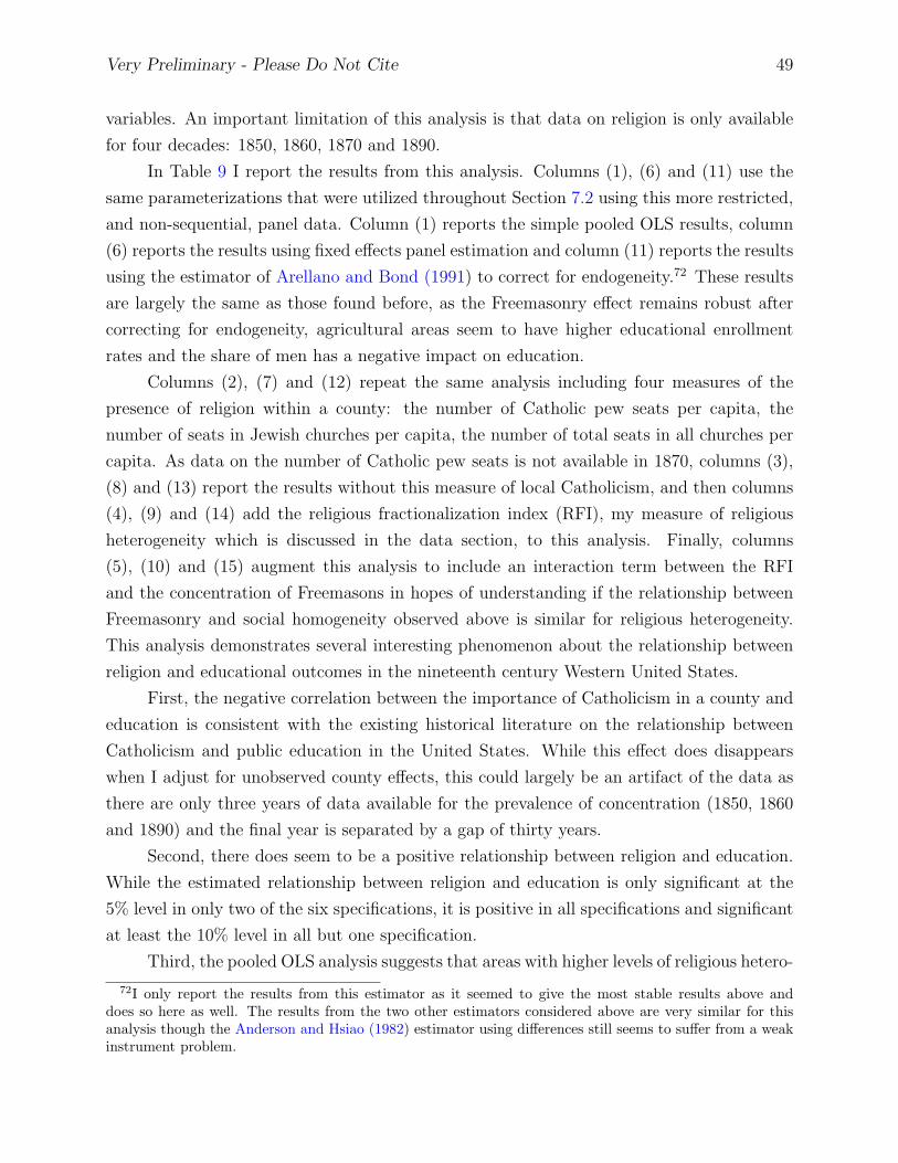
Very Preliminary - Please Do Not Cite 49
variables. An important limitation of this analysis is that data on religion is only available
for four decades: 1850, 1860, 1870 and 1890.
In Table 9 I report the results from this analysis. Columns (1), (6) and (11) use the
same parameterizations that were utilized throughout Section 7.2 using this more restricted,
and non-sequential, panel data. Column (1) reports the simple pooled OLS results, column
(6) reports the results using fixed effects panel estimation and column (11) reports the results
using the estimator of Arellano and Bond (1991) to correct for endogeneity.72 These results
are largely the same as those found before, as the Freemasonry effect remains robust after
correcting for endogeneity, agricultural areas seem to have higher educational enrollment
rates and the share of men has a negative impact on education.
Columns (2), (7) and (12) repeat the same analysis including four measures of the
presence of religion within a county: the number of Catholic pew seats per capita, the
number of seats in Jewish churches per capita, the number of total seats in all churches per
capita. As data on the number of Catholic pew seats is not available in 1870, columns (3),
(8) and (13) report the results without this measure of local Catholicism, and then columns
(4), (9) and (14) add the religious fractionalization index (RFI), my measure of religious
heterogeneity which is discussed in the data section, to this analysis. Finally, columns
(5), (10) and (15) augment this analysis to include an interaction term between the RFI
and the concentration of Freemasons in hopes of understanding if the relationship between
Freemasonry and social homogeneity observed above is similar for religious heterogeneity.
This analysis demonstrates several interesting phenomenon about the relationship between
religion and educational outcomes in the nineteenth century Western United States.
First, the negative correlation between the importance of Catholicism in a county and
education is consistent with the existing historical literature on the relationship between
Catholicism and public education in the United States. While this effect does disappears
when I adjust for unobserved county effects, this could largely be an artifact of the data as
there are only three years of data available for the prevalence of concentration (1850, 1860
and 1890) and the final year is separated by a gap of thirty years.
Second, there does seem to be a positive relationship between religion and education.
While the estimated relationship between religion and education is only significant at the
5% level in only two of the six specifications, it is positive in all specifications and significant
at least the 10% level in all but one specification.
Third, the pooled OLS analysis suggests that areas with higher levels of religious hetero-
72I only report the results from this estimator as it seemed to give the most stable results above anddoes so here as well. The results from the two other estimators considered above are very similar for thisanalysis though the Anderson and Hsiao (1982) estimator using differences still seems to suffer from a weakinstrument problem.

Very Preliminary - Please Do Not Cite 50
geneity have higher educational attainment. While the significance of this effect disappears
in the fixed effects panel analysis, a positive coefficient does remain. This is further evidence
that heterogeneity is not necessarily bad for the provision of public goods.
Finally, the interaction term between Freemasons and the RFI provides further evidence
that the benefit of Freemasonry was concentrated in heterogeneous areas. Indeed, the point
estimate for this interaction term is weakly positive - at the 10% level - in both the pooled
OLS results as well as the panel results that are corrected for endogeneity (following Arellano
and Bond (1991)).73
8.3 Freemasonry and Taxation
The hypothesized mechanism underlying the relationship between Freemasonry and the pro-
vision of education within a locality is that the presence of Freemasonry helped communities
overcome the common good problem. In this sub-section, I use taxation data to examine an
important prediction of this hypothesis. In particular, as schools were funded and provided
at primarily the village/city level, my hypothesis would predict that villages/cities with more
Freemasons would pay higher levels of local taxes, all other things equal.
I separate the analysis of taxation data into two sections as the taxation data that is
available is in two different forms. The first of these sections focuses on data from 1850 U.S.
Census which has data on the amount of funding for public schools from taxation and public
funds. Additionally, I look at the impact of Freemasonry on the number of public versus
private school teachers, which I argue is an indirect measure of the amount of wealth being
directed towards these two different types of schools. In this period, which corresponds to
the time during which the influence of Freemasonry was just beginning to expand, I find
no effect of Freemasonry on public funds or taxation. Additionally I find that areas with
more Freemasons were more likely to have fewer public teachers per capita and more private
teachers per capita, a result which is consistent with the result I found above.
Second I use data available for 1870 on the amount of local, county and state taxes paid
by each county. In this data, which corresponds to the period following the rapid expansion
of both the geographical spread as well as the concentration of Freemasonry, I find evidence
that regions with higher concentrations of Freemasons pay higher taxes of all kind, after
inclusion of a variety of controls for income, wealth and social homogeneity. Additionally, I
find that areas with more Freemasonry paid more local taxes as a share of total taxes than
other counties. As education funding was typically done at the village or local level for the
Western United States, this suggests that areas with more Freemasons where indeed more
73Both the concentration of Freemasons as well as the interaction term were treated as potentially endoge-nous variables for this analysis.
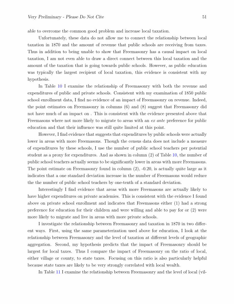
Very Preliminary - Please Do Not Cite 51
able to overcome the common good problem and increase local taxation.
Unfortunately, these data do not allow me to connect the relationship between local
taxation in 1870 and the amount of revenue that public schools are receiving from taxes.
Thus in addition to being unable to show that Freemasonry has a causal impact on local
taxation, I am not even able to draw a direct connect between this local taxation and the
amount of the taxation that is going towards public schools. However, as public education
was typically the largest recipient of local taxation, this evidence is consistent with my
hypothesis.
In Table 10 I examine the relationship of Freemasonry with both the revenue and
expenditures of public and private schools. Consistent with my examination of 1850 public
school enrollment data, I find no evidence of an impact of Freemasonry on revenue. Indeed,
the point estimates on Freemasonry in columns (6) and (8) suggest that Freemasonry did
not have much of an impact on . This is consistent with the evidence presented above that
Freemasons where not more likely to migrate to areas with an ex ante preference for public
education and that their influence was still quite limited at this point.
However, I find evidence that suggests that expenditures by public schools were actually
lower in areas with more Freemasons. Though the census data does not include a measure
of expenditures by these schools, I use the number of public school teachers per potential
student as a proxy for expenditures. And as shown in column (2) of Table 10, the number of
public school teachers actually seems to be significantly lower in areas with more Freemasons.
The point estimate on Freemasonry found in column (2), -0.20, is actually quite large as it
indicates that a one standard deviation increase in the number of Freemasons would reduce
the the number of public school teachers by one-tenth of a standard deviation.
Interestingly I find evidence that areas with more Freemasons are actually likely to
have higher expenditures on private academies. This is consistent with the evidence I found
above on private school enrollment and indicates that Freemasons either (1) had a strong
preference for education for their children and were willing and able to pay for or (2) were
more likely to migrate and live in areas with more private schools.
I investigate the relationship between Freemasonry and taxation in 1870 in two differ-
ent ways. First, using the same parameterization used above for education, I look at the
relationship between Freemasonry and the level of taxation at different levels of geographic
aggregation. Second, my hypothesis predicts that the impact of Freemasonry should be
largest for local taxes. Thus I compare the impact of Freemasonry on the ratio of local,
either village or county, to state taxes. Focusing on this ratio is also particularly helpful
because state taxes are likely to be very strongly correlated with local wealth.
In Table 11 I examine the relationship between Freemasonry and the level of local (vil-

Very Preliminary - Please Do Not Cite 52
lage), county and state taxation. In all cases, I find a positive, though not always significant,
relationship between the concentration of Freemasons and the level of taxation despite the
inclusion of a variety of controls for both local income and wealth as well as measures of so-
cial homogeneity. Interestingly, while the measures of local, agricultural and manufacturing,
have a positive relationship with taxation, income seems to have a negative effect when it
has an effect at all. Consistent with the model proposed by Goldin and Katz (1999), social
homogeneity as well as the number of people living in small towns have a positive impact
on county taxes. However, social homogeneity does not seem to effect either local or state
taxes.
Though the relationship between Freemasonry and taxes is highly significant (1% level)
for both county and state taxes, the relationship is much weaker for local taxes. Though
there is a significant overall impact at both the county and state level the effect seems to
be largely driven by the 10% of counties that derive at least two-thirds of their income
from manufacturing, though the relationship is still weakly positive in the more agricultural
regions. The weak effect observed for local taxes may be at least party driven by the fact
that nearly half of the localities reported having no local taxes. This downward censoring
may exclude many counties at an early stage of development where the Freemasonry impact
would potentially be particularly significant.
The evidence for the relationship between Freemason concentration and the ratio of
local to state taxes is a bit more mixed as is shown in Table 12. Indeed, while the relationship
seems to be positive for the ratio of village/city taxes to state taxes, there seems to be a
negative - though weak - impact on the county to state tax ratio. Interestingly, only one of
the two social capital measures suggested by Goldin and Katz has a significant effect and
is similar to the Freemasonry effect as it is only significant at the village level. Though the
Freemason variable only has a significantly positive effect among the manufacturing villages,
the effect among the more agricultural villages is still positive.
9 Robustness Checks
An important concern with the results presented above is that Freemasons are either (1)
migrating to areas that have higher provision of public education or (2) more likely to form
in areas with public education. In this section, I provide two types of robustness checks that
suggest that reverse causality is not driving the result that I observe.
I first examine the relationship between Freemasonry and education in the 1850. As
this early period corresponds to the very beginning of the spread of Freemasonry in the
West, and when the influence of Freemasonry was still quite weak, it allows me to explore

Very Preliminary - Please Do Not Cite 53
whether Freemasons were indeed more likely to migrate and form in areas with better public
education. Though I do find a weak positive relationship between Freemasonry and private
education during this period among counties with very high concentrations of Freemasonry,
this is evidence of Freemasons’ appreciation for education rather than the potential for a
community to a develop public education system (as suggested in Section 8).
I then explore the spread of Freemasonry in the West in more detail. This allows me
to examine the possibility that Freemasonry is simply functioning as a proxy for some other
economic variable. I demonstrate that the development of Freemasonry was not decisively
affected by any observable variables. As the spread of Freemasonry does not seem to have
been affected by important economic variables such as income and wealth, this is evidence
that Freemasonry is unlikely to be functioning as a proxy for some other variable.
9.1 Education in the Mid-19th Century
Both Freemasonry and educational enrollment data are relatively limited in the Western
United States in the mid-19th century. However, understanding the relationship between
Freemasonry and education in 1850 is an essential part of this analysis as Freemasonry
was just beginning to re-emerge in this year. Thus, if we observed a significant positive
relationship between Freemasonry and education in 1850, this would be strong evidence
that Freemasons were likely to migrate to areas with existing educational systems or that
Freemasons themselves had a positive impact independent of the organization.
However, there does not seem to a significant positive relationship between Freemasons
and total enrollment in 1850. This is demonstrated in column (2) of Table 16. Both columns
(1) and (2), which consider total enrollment within counties, indicate that income and wealth
have a positive impact and the one measure of social homogeneity that is available, the share
of the population in small towns, has a weak positive effect. Interestingly, a large adult male
population seems to be associated with low educational attainment, likely reflecting the
many frontier counties in these data.
These data also allow me to separately analyze the impact of Freemasonry on pub-
lic and private school enrollment. And while there is no significant relationship between
Freemasonry and enrollment in public schools, areas with higher concentration of Freema-
sons have significantly higher enrollment in private academies. As academies only account
for 3% of total enrollment during this period, this affect is muted when the date are pooled.
The estimated coefficient of ∼2 implies that for each additional Freemason that there are
two additional children in private academies. Though it is impossible to attach causality to
these estimates, this evidence is consistent with the strong preference among Freemasons for

Very Preliminary - Please Do Not Cite 54
education.
An important caveat to these results is that this analysis only considers data from
Arkansas, Illinois, Indiana, Missouri and Wisconsin. Though California, Iowa and Oregon
all have data available for this period, I excluded them from this analysis as most the
counties in these states were thinly populated. And though both Louisiana and Texas had
large, geographically distributed populations, I do not have Freemason data for these states
in 1850 as of yet.74
9.2 The Spread of Freemasonry
Freemasonry spread rapidly throughout the states of the Western United States during the
second half of the nineteenth century in terms of both size and geographical coverage as
shown in Figure 4. From a relatively small presence of only 0.2% of the population in 1850,
Freemasons accounted for over 1% of the population by 1870 - a share that was maintained
through 1900. The geographic spread of Freemasonry was equally impressive: while less than
half of the counties in 1850 had Freemasons, by 1900 Freemasons were present in all but 1%
of the counties of the Western United States. Though Freemasons were found throughout
the country, their concentration varied massively, from a low of 0.05% of the population to
upwards of 2 or even 5% of the population.
What explains the variation in the presence of Freemasons in a locality during the
nineteenth century? And what explains its rapid growth in the Western during this period
United States? In this section, I look at the possible influence of socioeconomic factors on
the spread of Freemasonry.
First, I explore what characteristics were correlated with a larger prevalence of Freema-
sonry and find that areas that had a larger religious presence and were more homogenous
had more Freemasons. Interestingly I find that the share of Catholics was negatively re-
lated to Freemasonry, as suggested by the historical literature, while the relationship with
Judaism was positive during the mid-19th century and became negative by the end of the
century. Finally, areas that were more religiously heterogeneous, as measured by a religious
fractionalization index that I construct here, had higher concentrations of Freemasons.
Second, as I am interested in understanding the determinants of Freemasonry, in addi-
tion to simply the characteristics that are correlated with Freemasonry, I turn to panel data
that will allow me to control for unobserved county heterogeneity. After controlling for this
potential heterogeneity, ethnic homogeneity has a negative effect on the presence of Freema-
sonry, the impact of religious heterogeneity disappears and for the first time a measure of
74These data were not available in the Iowa Masonic Library though I hope to obtain them in the future.

Very Preliminary - Please Do Not Cite 55
wealth - in this case, agricultural wealth - enters significantly. These latter results are robust
to correction for possible autocorrelation.
While the historical literature has proposed a variety of factors that may have been
correlated with the presence of Freemasonry, the lack of comprehensive quantitative data
in previous studies has made it difficult to test the relative importance of different factors.
In Table 13 I examine the relationship of a variety of potentially important socioeconomic
variables with Freemasonry. This table reports conditional correlations, which are calculated
by regressing the concentration of Freemasons against a variety of socioeconomic variables,
which are disaggregated by year so that I can examine the potentially changing character of
Freemasonry over time.
In columns (1)-(6) of Table 13 I focus on the relationship between Freemasonry and
several potentially important economic and demographic characteristics in 1850-1900. The
only effect that I find consistently across nearly all years in this analysis is that counties
with a larger population in agricultural areas, measured by either the share of population
living in urban areas (the opposite), the amount of agricultural capital or the amount of
agricultural output, are more likely to have more Freemasons. Suprisingly, despite the high
cost of joining the organization, which would suggest that wealthier areas would be likely to
have more Freemasons, I do not find evidence that total income or wealth are related to the
presence of Freemasonry.
The results from the first six columns of this table table also provide evidence that
the nature of the Freemasonry organization changed toward the end of the nineteenth cen-
tury as suggested by Tabbert (2005) and others. The most striking piece of evidence that
Freemasonry was evolving from an exclusive organization into a social club between the late
1880s and the turn of the century is that the importance of the share of men as a correlate
of Freemasonry changes dramatically between 1890 and 1900. Though one might expect
that Freemasons would be more prevalent in areas with more men, as there would be more
potential candidates, in practice the family is a very important of being a Freemason. Thus,
while the relationship between Freemasonry and the share of men is weakly positive and
stable from 1850-1890, the large increase in both the point estimate and significance of this
variable is consistent with the evolution of Freemasonry into a ‘club for men’.
The relationship between Freemasonry and religion is explored in columns (7)-(10)
of Table 13. While my empirical approach does not allow me to identify the faiths of
Freemasons themselves, I can examine the religious composition of the communities where
Freemasonry is most prevalent. In all years for which there is religious I find that counties
with a larger religious presence, as measured by the total number of seats in all churches,
have more Freemasons as a share of the local population. This likely reflects either the

Very Preliminary - Please Do Not Cite 56
complementarity of these social institutions or the importance of religion to Freemasons.
The antagonistic relationship between the Catholic Church and Freemasonry is sup-
ported by the negative relationship found between the importance of a Catholic Church in
an area and the importance of Freemasonry. Interestingly, while a similar relationship was
found during the later part of this period for the Jewish faith, a positive relationship is
observed between the importance of Judaism and Freemasonry in 1850. This result, which
is robust to the exclusion of communities with the highest concentrations of Jewish seats per
capita, indicates that Freemasonry spread particularly in areas that were Jewish in an early
period. While this could reflect a relationship between Judaism and Freemasonry, it more
likely reflects the urban nature of Freemasonry as the concentration of Jews in an area is a
better measure of urbanization than the share of the population in cities with over 25,000
people.
Interestingly, religious fractionalization, which is a measure of the religious heterogene-
ity of a county as discussed in the data section above, seems to have a very strong positive
relationship with Freemasonry during 1850-1870. This is perhaps an unusual finding. How-
ever, it is consistent with the fact that Freemasonry’s impact seems to be more important
in heterogeneous areas.
This positive relationship between Freemasonry and religious fractionalization disap-
pears in 1890. I also find that the share of the population of native parentage, a share
of ethnic homogeneity, increases during this period. Though this analysis is not sufficient
to make any strong claims, this does give provide some evidence about the nature of the
transition that the Freemasonry organization experienced in the late nineteenth century.
In particular, as the organization lost its elite character and became more inclusive it also
became more nativist and homogenous.
In the above sub-section, I examine the correlation between a variety of socioeconomic
characteristics and Freemasonry. While these correlations are interesting in their own right,
as they provide valuable information about the type of communities where Freemasonry
was more prevalent, these previous estimates should not be interpreted as measures of the
impact of these different factors on the presence of Freemasonry. In particular it is likely that
there are unobservable variables, such as the amount of ‘social capital’ in a community, that
is likely to influence both the concentration of Freemasonry and some of the explanatory
variables. In this section, I will use a panel data approach to compensate for the potentially
confounding effect of unobserved county heterogeneity.
The approach is straightforward. The share of the population that is Freemason in

Very Preliminary - Please Do Not Cite 57
county i and at time t, Fit, is modeled as
Fit = X ′itβ + ωi + εit (10)
where Xit is a variety of socioeconomic variables that are likely to affect Freemasonry, ωi is
a fixed effect that is possibly correlated with Xit and εit is a stochastic shock. Equation (10)
is then estimated using three different sets of panel data. The first of these data sets has the
most coverage in terms of time, spanning from 1850-1900, but contains the least geographic
coverage as it uses the earliest available county definitions which tend to be more aggregated
than later counties (T = 6, N = 451). The third data set covers the fewest years, only 1870-
1900, but offers the greatest geographical variation (T = 4, N = 1034) while the second,
which covers 1860-1900, is a balance between geographical variation and years covered (T =
5, N = 843).
Table 14 reports the results from the simplest estimate of equation (10) which are
broadly consistent with the results found above. Columns (1)-(3) report standard OLS esti-
mates using the data constructed for the panel estimation, which are calculated to demon-
strate the comparability of these data will the previous data, while columns (4)-(6) report
results from fixed effects panel estimation. These fixed effects estimates show that the im-
portance of agricultural in an area has a positive impact on the development of Freemasonry,
which was suggested in the above analysis using conditional correlations. However, while the
above correlational analysis indicated that communities with higher ethnic homogeneity had
higher levels of Freemasonry, especially in a later period, the results from columns (4)-(6)
suggest that this homogeneity has a negative impact, if any, on the share of Freemasons.
Columns (7) and (8) of Table 14 also provide weak evidence that the point estimates
for the religious variables in the conditional correlations reported in the previous sub-section
may have a causal interpretation. While the point estimates on the Freemason variables are
never significant, identification is difficult as the level of religiosity and its heterogeneity does
not vary significantly over the 40 year horizon that is covered by these data.
A contention that may be raised with the estimation of equation (10) is that it ignores
the possibility of autocorrelation in the Freemasonry variable. Indeed, as lodges require the
presence of other Freemasons in an area to open and expand it is likely that areas with more
Freemasons in one period are likely to have more Freemasons in the subsequent period.
In order to both correct for the possible bias due to ignoring this autocorrelation, as
well as to estimate the correlation of the concentration of Freemasonry across decades, I thus

Very Preliminary - Please Do Not Cite 58
estimate
Fit = αFi,t−1 +X ′itβ + ωi + εit (11)
where Fi,t−1 is the lagged level of the concentration of Freemasons in a county and the
rest of the notation is the same as before. As my panel data has only 4-6 periods of data,
depending on the data set used, I face the classic “small T” problem and standard approaches
for estimating the AR1 model are not available. Thus I estimate equation (11) using the
approaches of Anderson and Hsiao (1982) and Arellano and Bond (1991) which are discussed
in more detail in Section 7.2 below.
Table 15 reports the results from the analysis that adjusts for the possibility of auto-
correlation in the dependent variable. Columns (1)-(6) report the results for each of the two
estimators for the three possible panel data sets. In each I find that there is a significant
degree of autocorrelation. While the point estimates vary from 0.10-0.50 across the various
samples and specifications, the fact that the point estimate is always positive and significant
(usually at the 1% level) indicates that the presence of Freemasonry in a county has an
impact on Freemasonry in that county a decade later.75
Interestingly, once I correct for this this autocorrelation, the estimates of the impact of
the concentration of adult males becomes very strong and significant. Indeed, I find evidence
that communities that have a large concentration of adult males are less likely to have large
Freemason communities. This result, which is significant across all specifications, indicates
that the presence of families was a driving factor in the expansion of the organization in the
West.76
A similar analysis for the panel data that includes religious variables does not produces
any new significant results. However, these results, which are presented in columns (7)-(8)
of Table 15, do demonstrate the robustness of the negative relationship between the share
of males in a county and the prevalence of Freemasonry.
10 Conclusion
In this paper I explored the role that American Freemasonry played in the development
of the educational system in the United States. Using a novel panel data set of American
Freemasonry during the 19th century, I documented that counties with higher concentrations
of Freemasons had higher primary school enrollment rates in the late 19th century. And
75If I restrict the sample to only counties with non-zero Freemasons, I find a very similar effect.76An identical result is found using data restricted to counties with non-zero Freemasons.

Very Preliminary - Please Do Not Cite 59
the impact of Freemasonry was quite important: a one standard-deviation increase in the
concentration of Freemasons was equivalent to a one-fourth of a standard-deviation increase
in the primary school enrollment rate. The availability of panel data for both enrollment
rates and Freemasonry allowed me to rule out both reverse causality and endogeneity as
possible explanations for this observed effect.
And, in what is a striking example of path dependence, I showed that the concentration
of Freemasonry in the 19th century also had a significant positive impact on secondary school
enrollment in the beginning of the following century. This result is particular significant given
that most reports indicate that the influence of Freemasonry had largely waned by the end
of the 19th century.
The evidence presented here indicate that Freemasonry impacted the American ed-
ucation system by helping communities attenuate the common good problem. This was
demonstrated in two ways. First, the impact of Freemasonry was particularly meaningful in
areas that typically suffer the most from common good problems, i.e. those that were the
most heterogeneous ethnically and religiously. Second, counties with higher concentrations
of Freemasons had higher levels of local taxation. This result, which is consistent with both
the rhetoric of Freemasons and other historical studies of Freemasons, indicates the powerful
development impact that a social institution with a relatively small number of individuals
can have.

Very Preliminary - Please Do Not Cite 60
References
Alesina, A. and E. L. Ferrara (2005). Ethnic diversity and economic performance. Journal
of Economic Literature 43 (3), 762–800.
Anderson, T. W. and C. Hsiao (1982). Formulation and estimation of dynamic models
using panel data. Journal of Econometrics (18), 47–82.
Arellano, M. and S. Bond (1991). Some specification tests for panel data: Monte carlo
evidence and an application to employment equations. Review of Economic Studies 58,
277–298.
Black, S. E. and K. L. Sokoloff (2006). Long-term Trends in Schooling: The Rise and
Decline (?) of Public Education in the United States. In E. A. Hanusek and F. Welch
(Eds.), Handbook of the Economics of Education, Volume 1, Chapter 2.
Boli, J., F. O. Ramirez, and J. W. Meyer (1985). Explaining the origins and expansion of
mass education. Comparative Education Review 29 (2), 145–170.
Braggion, F. (2009, March). Social networks eects on listed and unlisted firms: Evidence
from managers aliations with freemasonry. Mimeo.
Burt, R. (2003). Freemasonry and business networking during the victorian period. Eco-
nomic History Review LVI (4), 657–688.
Chandler, A. (1977). The Visible Hand. Cambridge, Mass. and London, England: The
Belknap Press of Harvard University Press.
Clark, G. B. (1936). Our Masonic Heritage: A Glimpse of the Historical Background of
Freemasonry. Denver: Grand Lodge A.F. and A.M. of Colorado.
Cohen-Zada, D. and M. Justman (2003). The political economy of school choice: linking
theory and evidence. Journal of Urban Economics 54, 277–308.
Cubberley, E. (1920). The History of Education. Houghton Mifflin Company.
Cubberley, E. (1922). A Brief History of Education: A History of the Practice and Progress
and Organization of Education. Houghton Mifflin Company.
Davis, J. S. (1917). Essays in the Earlier History of American Corporations. Harvard
University Press.
De Los Reyes, G. and A. Lara (1999). Civil society and volunteerism. ANNALS,
AAPSS 565.
Demott, B. J. (1986). Freemasonry in American Culture and Society. University Press of
AMerica.

Very Preliminary - Please Do Not Cite 61
Denzau, A. and K. Grier (1984). Determinants of local school spending: Some consistent
estimates. Public Choice 44, 375–383.
Dexter, E. (1904). A History of Education in the United States. The Macmillan company.
Dumenil, L. (1984). Freemasonry and American Culture 1880-1930. Princeton University
Press.
Dumenil, L. (1990). “The Insatiable Maw of Bureaucracy”: Antistatism and Education
Reform in the 1920s. The Journal of American History 77 (2), 499–524.
Easterlin, R. A. (1960). Interregional differences in per capita income, population, and
total income, 1840-1950. In Conference on Research in Income and Wealth, Trends
in the American Economy in the Nineteenth Century, Studies in Income and Wealth,
Volume 24, pp. 73–140. Princeton University Press.
Eby, F. (1925). The Development of Education in Texas. New York: The MacMillan
Company.
Epple, D. and R. E. Romano (1996). Ends against the middle: Determining public service
provisions when there are private alternatives. Journal of Public Economics 62, 297–
325.
Fels, T. (2002). Religious assimilation in a fraternal organization. In R. Weisberger,
W. McLeod, and S. Morris (Eds.), Freemasonry on Both Sides of the Atlantic: Es-
says Concering the Craft in the British Isles, Europe, the United States and Mexico.
Columbia University Press.
Fox, W. L. (1997). Lodge of the Double-Headed Eagle: Two Centuries of Scottish Rite
Freemasonry in America’s Southern Jurisdiction. University of Arkansas Press.
Go, S. (2008). Free schools in america, 1850-1870: Who voted for them, who got them,
and who paid. Job Market Paper, University of California, Davis .
Go, S. and P. H. Lindert (2008, November 10). The Curious Dawn of American Public
Schools. University of California - Davis.
Goldin, C. and L. F. Katz (1998, May). The origins of state-level differences in the public
provision of higher education: 1890-1940. The American Economic Review , 303–308.
Goldin, C. and L. F. Katz (1999). Human capital and social capital: The rise of secondary
schooling in america, 1910-1940. Journal of Interdisciplinary History XXIX (4), 683–
723.
Goldin, C. and L. F. Katz (2003). Mass secondary schooling and the state: The role of
state compulsion in the high school movement. NBER Working Paper # 10075.

Very Preliminary - Please Do Not Cite 62
Goldin, C. and L. F. Katz (2008). Why the United States Led in Education: Lessons from
Secondary School Expansion, 1910 to 1940.
Goldsmith, R. W. (1952). The Growth of Reproducible Wealth of the United States of
America from 1805 to 1950. Review of Income and Wealth 2 (1), 247–328.
Greif, A. (1993). Contract Enforceability and Economic Institutions in Early Trade: the
Maghribi Traders’ Coalition. American Economic Review 83 (3), 525–48.
Harland-Jacobs, J. (2007). Builders of Empire: Freemasons and British Imperialism, 1717-
1927. UNC Press.
Haywood, H. L. (1963). The Masonic Essays of H. R. Haywood, Volume 20. Fulton: Trans-
actions of the Missouri Lodge of Research.
Hope, K. G. (2005). “One Can Make A Difference”. The California Encompasser 19 (4).
Kutolowski, K. S. (1982). Freemasonry and community in the early republic: The case for
antimasonic anxieties. American Quarterly 34, 543–561.
Kuznets, S. (1946). National Product Since 1869. (Assisted by Lillian Epstien and Eliza-
beth Jenks). National Bureau of Economic Research.
Lang, O. (2006). History of Freemasonry in the State of New Yor. Kessinger Publishing.
Lindert, P. H. (2004). Growing public : social spending and economic growth since the
eighteenth century. Cambridge University Press.
Mackey, A., R. Clegg, and H. Haywood (1946). Encyclopedia of Freemasonry. Kessinger
Publishing.
Mackey, A. and H. Haywood (2003). Encyclopedia of Freemasonry Part 2. Kessinger Pub-
lishing.
Moore, C. (1846). The Freemasons’ Monthly Magazine.
Parry, D. L. L. (1998). Friends in high places: The favours sought by the freemasons of
orleans, 1890-1914. French History 12 (2).
Pike, A. (1871). Morals and dogma of the Ancient and Accepted Scottish Rite of Freema-
sonry. Masonic Publishing Company.
Poterba, J. M. (1997). Demographic structure and the political economy of public educa-
tion. Journal of Policy Analysis and Management, 16 (1), 48–66.
Rosenzweig, R. (1977). Boston masons, 1900-1935: the lower middle class in a divided
society. Nonprofit and Voluntary Sector Quarterly 6 (119).

Very Preliminary - Please Do Not Cite 63
Royal Arch Masons of California (1882). Proceedings of the Grand Chapter of Royal Arch
Masons of the State of California at Its Annual Convocation. Royal Arch Masons of
California: Royal Arch Masons, Grand Chapter.
Ruggles, S., J. T. Alexander, K. Genadek, R. Goeken, M. B. Schroeder, and M. Sobek
(2010). Integrated public use microdata series: Version 5.0 [machine-readable
database]. Technical report, Minneapolis: University of Minnesota.
Seaman, E. C. (1868). Essays on the Progress of Nations, in Civilization, Productive Indus-
try, Wealth and Population: Illustrated by Statistics of Mining, Agriculture, Manufac-
tures, Commerce, Coin, Banking, Internal Improvements, Emigration, and Population.
C. Scriber & Co.
Soltow, L. and E. Stevens (1981). The Rise of Literacy and the Common School in the
United States. University of Chicago Press, Chicago.
Stillson, H. L. and W. J. Hughan (1890). History of the Ancient and Honorable Frater-
nity of Free and Accepted Masons, and Concordant Orders. The Fraternity publishing
company.
Tabbert, M. A. (2005). American Freemasons: Three Centuries of Building Communities.
National Heritage Museum and New York University Press.
Thornton, J. (1962). The Contributions of Freemasonry in Texas to Public School Educa-
tion, 1846 to 1861. Master’s thesis, Baylor University, Waco.
Thornton, J. (1970). The Relationship of Freemasonry to the Structure, Organization,
and Administration of Public School Education in Texas, 1861-1885. Texas A & M
University.
Tucker, G. (1843). Progress of the United States in Population and Wealth in Fifty Years,
as Exhibited by the Decennial Census: As Exhibited by the Decennial Census. Little &
Brown.
Vigdor, J. L. (2004). Community composition and collective action: Analyzing initial mail
response to the 2000 census. The Review of Economics and Statistics 86 (1), 303–312.
Webb, W. (1955). Masonry in Texas, Background, History and Influence in 1846. Fort
Worth: The Masonic Home and School Press.
Weber, M. (1946). The Protestant Sects and the Spirit of Capitalism. New York: Oxford
University Press.
Whitsell, L. O. (1950). One Hundred Years of Freemasonry in California. Grand Lodge
F. & A. M. of California.

Very Preliminary - Please Do Not Cite 64
Woods, R. O. (1936). Masonic educational institutions. The School Review 44 (6), 456–461.
Wooldridge, J. (2002). Econometric Analysis of Cross Section and Panel Data. The MIT
Press.

Very Preliminary - Please Do Not Cite 65
A Appendix of Proofs, etc. for the Model
(This is not very complete at all - the results that I need to prove are very simple though)
Assumption A1. Educational services are a normal (or superior good). [Same as Epple
and Romano]
Assumption A2. For x > 0, b > 0, x and b ≥ 0, U(x, b, aE > U(0, b, aE) and
U(x, b, aE > U(x, 0, aE)
Assumption A3. I need some sort of assumption over the last term. I’ll come back to
that later.
Skip a bunch of stuff so that I can work on 5.
A household that consumes private school services chooses x to maximize U(x, b, aE)
subject to the budget constraint y(1− t) = px+ b. Let
v(p, y(1− t), aE) = maxx
U(x, y(1− t)− px, aE). (12)
Define x∗ as the solution to equation (12).
A household with public schooling obtains utility
U(E, y(1− t), aE). (13)
Now, the first thing to do is take a look at the line of (E, t) that makes an individual
indifferent between private and public education. That is I want to take a look at all points
such that
v(p, y(1− t), aE) = U(E, y(1− t), aE) (14)
which is equivalent to looking at U(x∗, y(1−t)−px∗, aE) = U(E, y(1−t), aE). For notational
simplicity, define Ux∗ = U(x∗, y(1− t)− px∗, aE), U = U(E, y(1− t), aE).
OK, now I need to create my version of their equation (5). To do this, I just take the
total derivative of equation (14) and solve for dtdE
:
−y · Ux∗
2 · dt+ a · Ux∗
3 · dE = U1 · dE +−y · U2 · dt+ a · U3 · dE (15)
dt
dE=U1 + a · (U3 − Ux∗
3 )
y(U2 − Ux∗2 )
(16)
Note that equation (16) is equivalent to Epple and Romano if a = 0. Also, I will maintain

Very Preliminary - Please Do Not Cite 66
the assumption that a is defined such that
U1 + a · (U3 − Ux∗
3 ) > 0 (17)
which is true for some positive and negative a in a neighborhood of a = 0. This will guarantee
me that (16) < 0 following the same argument as Epple and Romano.
(Insert new drawings looking at what happens for a > 0 - i.e. Freemasons.)
Now I will reproduce their Lemma 1. I’ll just do the “math”.
(1− t) · Ux∗
2 · dy + a · Ux∗
3 · dE = U1 · dE + (1− t) · U2 · dy + a · U3 · dE (18)
dE
dy=
(1− t)(U2 − Ux∗2 )
−U1 − a · (U3 − Ux∗3 )
> 0 (19)
The inequality in (19) follows from the fact that the denominator is negative from equation
(17) and the enumerator is also negative following Epple and Romano.
A further result that is of much interest to me, and will drive my central result is thatdEda> 0. This can be shown as
a · Ux∗
3 · dE + E · Ux∗
3 · da = U1 · dE + a · U3 · dE + E · U3 · da (20)
dE
da=
E(U3 − Ux∗3 )
−U1 − a · (U3 − Ux∗3 )
> 0 (21)
The inequality in (21) follows from the fact that the enumerator is negative if I assume that
DMU of Epple and Romano hold for this third argument and the numerator is negative from
(17).
. . .
I will need two assumptions to show this result:
Assumption H1: Individuals in heterogeneous communities are more likely to have a
negative α.
Assumption H2: The magnitude of this negative value of α is increasing in the level of
heterogeneity in a community.
Case 1: The α of the household with income yH becomes more negative.Result: Educational expenditures, taxation and enrollment will fall.
Proof: If yH remains the wealthy household determining the equilibrium, this
result will clearly hold as shown in Figure 6(b). If yH is no longer the equilibrium
than a household with income y′H < yH will determine the equilibrium. There can
not exist a y > y∗H that will determine an equilibrium as the previous equilibrium
was assumed to be unique.

Very Preliminary - Please Do Not Cite 67
Case 2: The α of the household with income yH is unchanged, but individuals with
wealth greater than yH experience a larger negative α which leads to an equivalent income
below yH .Result: Educational expenditures, taxation and enrollment will fall.
Sketch of Proof: Similar to above.
Case 3: The α of the households with income ≥ yH and ≤ yL are unchanged, but
individuals with wealth in this range experience a larger negative α which does not shift
their equivalent past either yH or yL.Result: Educational expenditures, taxation and enrollment are not affected.
Sketch of Proof: Neither yL nor yH nor∫ yh
ylf(y)dy are affected.
Case 4: The α of a household with income y > yL experiences a fall in α which shifts
its equivalent income past yL.Result: Educational expenditures, taxation and enrollment will fall.
Sketch of Proof:∫ yh
ylf(y)dy becomes less than 0.5. The equilibrium will shift to
the intersection of the indifference curves of households with incomes just below
yL and just below yH .
Case 5: The α of the household with income yL experience a larger negative α.Result: Educational expenditures, taxation and enrollment will fall.
Sketch of Proof: Similar to Case 1.

Very Preliminary - Please Do Not Cite 68
B Freemason Data
1850 1860 1870 1880 1890 1900
Arizona 1912 1870 1866 1882 X X X X Arkansas 1836 1850 1835 1837 X X X X X ??California 1850 1850 1850 1850 X X X X X X Colorado 1876 18601 1860 1861 X X X X X Idaho 1890 1870 1863 1867 X X ?? X Illiois 1818 1850 1838 1840 X X X X X X Indiana 1816 1850 1807 1818 X X X X X X Iowa 1846 1850 1840 1841 X X X X X X Kansas 1861 1860 1854 1856 X X X X X Louisiana 1812 1850 1794 1812 ?? X X X X X Minnesota 1858 1850 1852 1853 X X X X X Missouri 1821 1850 1808 1821 X ?? X X X X Montanta 1889 1870 1864 1866 X X X X Nebraska 1867 1860 1855 1857 X X X X X Nevada 1864 1860 1864 1866 X X X X New Mexico 1912 1850 1851 1879 ** X X X X North Dakota 1889 1870 18742 1890 X X X Oregon 1859 1850 1848 1851 X X X X X X South Dakota 1889 1860 1863 1875 X X X X Texas 1845 1850 1836 1838 ?? X X X ‡ ??Utah 1896 1850 18663 1872 X X X X Washington 1889 1860 1852 1858 X X X X X X Wisconsin 1848 1850 1843 1843 X X X X X X Wyoming 1890 1870 1868 1874 X X X X
Economic Data First AvailableState Founded First Lodge†
Grand Lodge Established
Years for Which Freemason Data is
Available
Notes:??: Data is in principle available but was not available at the Iowa Masonic Library.**: Only one lodge was open in New Mexico in 1860 (under the jurisdiction of the GrandLodge of Missouri). The data for this year was estimated as half that of 1870. As the 1860Freemason is not used for quantitative analysis, this assumption does not affect any of theresults (just the map).‡: Data for Texas was not available for 1890. 1888 was the last year for which Freemasonmembership data was available.†: There was often a difference of a year or more between the data in which a lodge wasestablished and which it was chartered.[1]: There is only very limited data available for Colorado in 1860 - only one county withdata.[2]: There was one lodge formed slightly earlier, but it was closed.[3]: There was a lodge formed significantly earlier, in 1858, but it was disbanded.
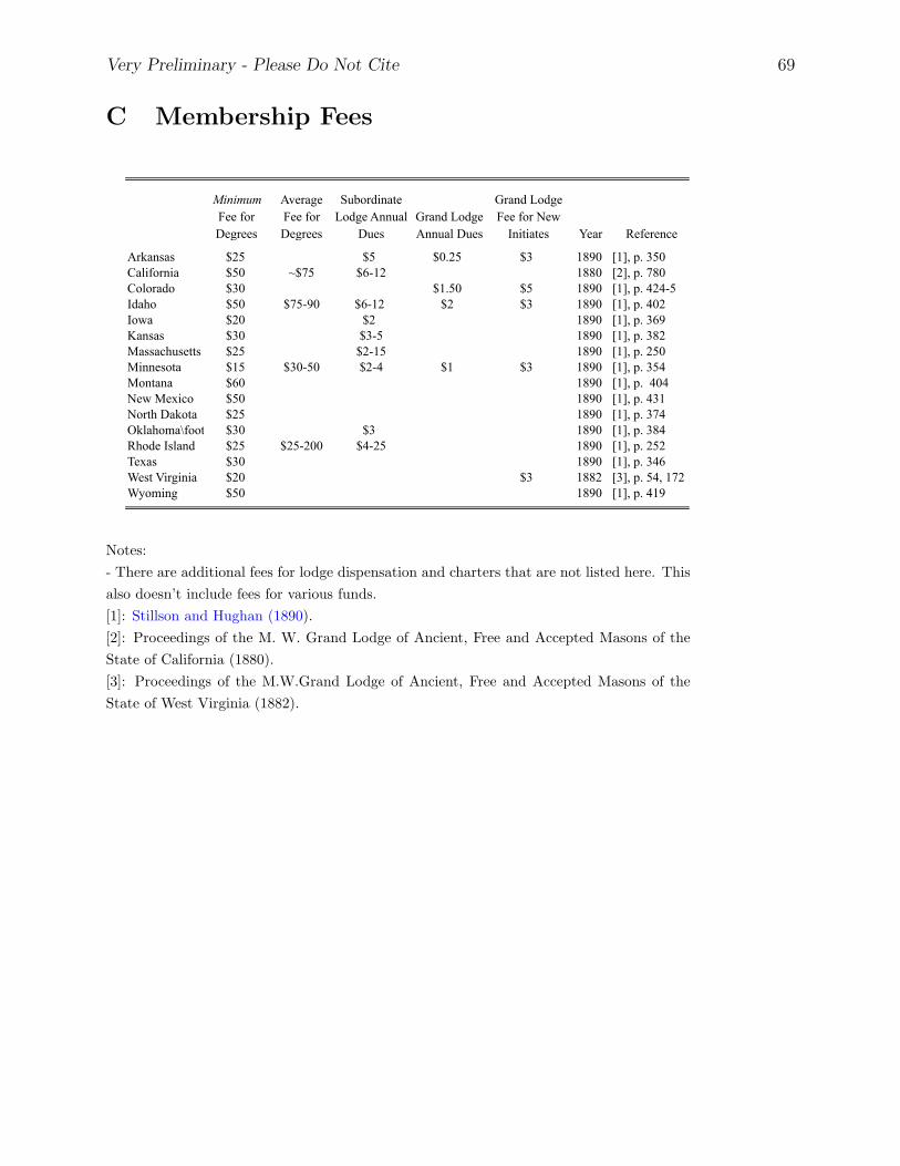
Very Preliminary - Please Do Not Cite 69
C Membership Fees
Minimum Fee for Degrees
Average Fee for Degrees
Subordinate Lodge Annual
Dues Grand Lodge Annual Dues
Grand Lodge Fee for New
Initiates Year Reference
Arkansas $25 $5 $0.25 $3 1890 [1], p. 350California $50 ~$75 $6-12 1880 [2], p. 780 Colorado $30 $1.50 $5 1890 [1], p. 424-5Idaho $50 $75-90 $6-12 $2 $3 1890 [1], p. 402Iowa $20 $2 1890 [1], p. 369Kansas $30 $3-5 1890 [1], p. 382Massachusetts $25 $2-15 1890 [1], p. 250Minnesota $15 $30-50 $2-4 $1 $3 1890 [1], p. 354Montana $60 1890 [1], p. 404New Mexico $50 1890 [1], p. 431North Dakota $25 1890 [1], p. 374Oklahoma\footnote{Called the Indian Territory during this period.} $30 $3 1890 [1], p. 384Rhode Island $25 $25-200 $4-25 1890 [1], p. 252Texas $30 1890 [1], p. 346West Virginia $20 $3 1882 [3], p. 54, 172Wyoming $50 1890 [1], p. 419
Notes:- There are additional fees for lodge dispensation and charters that are not listed here. Thisalso doesn’t include fees for various funds.[1]: Stillson and Hughan (1890).[2]: Proceedings of the M. W. Grand Lodge of Ancient, Free and Accepted Masons of theState of California (1880).[3]: Proceedings of the M.W.Grand Lodge of Ancient, Free and Accepted Masons of theState of West Virginia (1882).

Very Preliminary - Please Do Not Cite 70
Figure 1: National Prominence of American Freemasonry

Very Preliminary - Please Do Not Cite 71
Figure 2: Freemason Capital Relative to Total Physical Capital
(state means and standard deviations)

Very Preliminary - Please Do Not Cite 72
Figure 3: GDP per capita and the Cost of Freemasonry
(state means and standard deviations)

Very Preliminary - Please Do Not Cite 73
Figure 4: Spread of Freemasonry in the Western United States
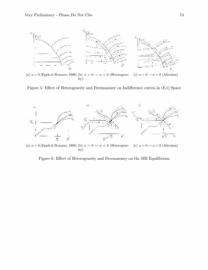
Very Preliminary - Please Do Not Cite 74
(a) α = 0 (Epple & Romano, 1996) (b) α = 0 → α < 0 (Heterogene-ity)
(c) α = 0→ α > 0 (Altruism)
Figure 5: Effect of Heterogeneity and Freemasonry on Indifference curves in (E,t) Space
(a) α = 0 (Epple & Romano, 1996) (b) α = 0 → α < 0 (Heterogene-ity)
(c) α = 0→ α > 0 (Altruism)
Figure 6: Effect of Heterogeneity and Freemasonry on the SRI Equilibrium

Very Preliminary - Please Do Not Cite 75
Figure 7: Freemasons in the Western United States: 1850
Figure 8: Freemasons in the Western United States: 1860

Very Preliminary - Please Do Not Cite 76
Figure 9: Freemasons in the Western United States: 1870
Figure 10: Freemasons in the Western United States: 1880
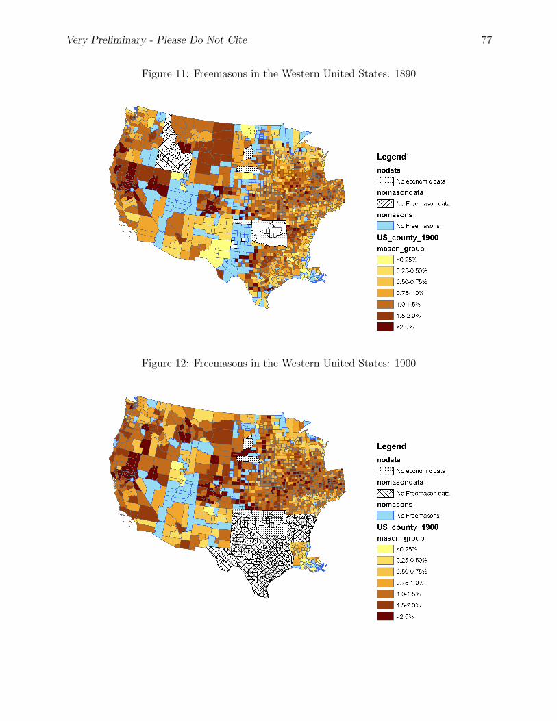
Very Preliminary - Please Do Not Cite 77
Figure 11: Freemasons in the Western United States: 1890
Figure 12: Freemasons in the Western United States: 1900

Very Preliminary - Please Do Not Cite 78
Tab
le1:
Fre
emas
onry
and
Educa
tion
inth
eL
ate-
19th
Cen
tury
(1)
(2)
(3)
(4)
(5)
(6)
(7)
(8)
(9)
(10)
< 33
%33
-66%
> 66
%<
33 %
33-6
6%>
66%
0.03
**0.
02**
0.03
*0.
000.
01-0
.01
-0.0
1-0
.02
-0.0
7***
0.05
(0.0
1)(0
.01)
(0.0
2)(0
.03)
(0.0
3)(0
.01)
(0.0
1)(0
.01)
(0.0
2)(0
.03)
0.00
0.01
0.02
-0.0
40.
000.
010.
020.
010.
040.
04(0
.01)
(0.0
1)(0
.02)
(0.0
4)(0
.03)
(0.0
1)(0
.01)
(0.0
1)(0
.03)
(0.0
3)0.
010.
000.
00-0
.00
0.07
**0.
000.
000.
000.
04**
-0.0
3(0
.01)
(0.0
1)(0
.02)
(0.0
2)(0
.03)
(0.0
1)(0
.01)
(0.0
1)(0
.02)
(0.0
3)0.
02**
0.03
**0.
03**
0.07
***
-0.0
50.
010.
000.
020.
00-0
.02
(0.0
1)(0
.01)
(0.0
1)(0
.02)
(0.0
4)(0
.01)
(0.0
1)(0
.02)
(0.0
3)(0
.04)
0.17
**0.
13*
0.00
0.18
*0.
38**
0.43
***
0.39
***
0.42
***
0.48
***
0.20
(0.0
7)(0
.07)
(0.0
8)(0
.11)
(0.1
9)(0
.05)
(0.0
5)(0
.06)
(0.0
9)(0
.13)
-0.0
00.
040.
000.
000.
02-0
.08*
**-0
.07*
*0.
000.
00-0
.07*
(0.0
9)(0
.08)
..
(0.1
0)(0
.03)
(0.0
3).
.(0
.04)
0.03
***
0.02
***
0.02
*0.
020.
02-0
.01
-0.0
00.
01-0
.02
-0.0
1(0
.01)
(0.0
1)(0
.01)
(0.0
2)(0
.02)
(0.0
1)(0
.01)
(0.0
1)(0
.01)
(0.0
1)-0
.07
-0.0
7-0
.47*
*0.
130.
29-0
.37*
**-0
.41*
**-0
.65*
**-0
.38
0.33
(0.1
2)(0
.12)
(0.2
0)(0
.20)
(0.2
3)(0
.13)
(0.1
2)(0
.12)
(0.2
4)(0
.23)
3.77
***
4.01
***
3.22
**2.
033.
63**
*3.
54**
*3.
78**
*3.
17(0
.75)
(0.9
3)(1
.48)
(1.7
6)(0
.74)
(0.9
0)(1
.25)
(2.3
9)R
20.
590.
610.
620.
660.
440.
400.
410.
410.
530.
40N
=
1012
1012
660
231
121
1304
1304
849
285
170
log(
KM
per
cap
ita)
1870
1890
% o
f Men
ove
r 21
# M
ason
s / T
otal
Pop
ulat
ion
Shar
e of
Out
put f
rom
log(
KA p
er c
apita
)
Prop
ortio
n of
pop
ulat
ion
nativ
e bo
rn
Prop
ortio
n of
pop
ulat
ion
in to
wns
with
<
25,0
00 p
eopl
e
log(
popu
latio
n)
Shar
e of
Out
put f
rom
log(
YM
per
cap
ita)
log(
YA p
er c
apita
)
Note
s:C
olu
mn
s(3
)an
d(8
)in
clu
de
cou
nti
esw
ith≤
33%
of
ou
tpu
tfr
om
manu
fact
uri
ng,
(4)
an
d(9
)are
cou
nti
esw
ith
34-6
6%
of
ou
tpu
tfr
om
manu
fact
uri
ng
an
d(5
)an
d(1
0)
incl
ud
eco
unti
esw
ith≥
67%
of
ou
tpu
tfr
om
manu
fact
uri
ng.
All
spec
ifica
tion
sin
clu
de
state
fixed
effec
ts.
Rob
ust
stan
dard
erro
rsin
pare
nth
eses
.
1:
For
1890,
this
vari
ab
leis
the
“P
op
ula
tion
of
Pop
ula
tion
Nati
ve
Born
,w
ith
Nati
ve
Pare
nta
ge”
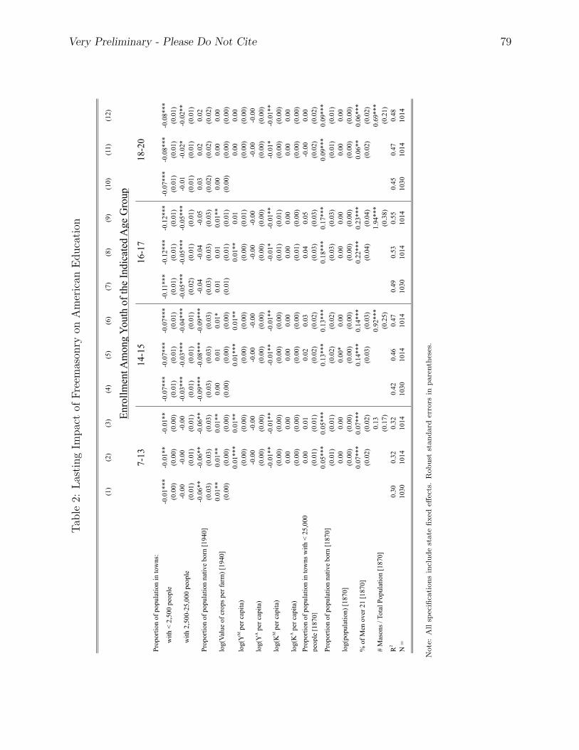
Very Preliminary - Please Do Not Cite 79
Tab
le2:
Las
ting
Impac
tof
Fre
emas
onry
onA
mer
ican
Educa
tion
(1)
(2)
(3)
(4)
(5)
(6)
(7)
(8)
(9)
(10)
(11)
(12)
Prop
ortio
n of
pop
ulat
ion
in to
wns
:-0
.01*
**-0
.01*
*-0
.01*
*-0
.07*
**-0
.07*
**-0
.07*
**-0
.11*
**-0
.12*
**-0
.12*
**-0
.07*
**-0
.08*
**-0
.08*
**(0
.00)
(0.0
0)(0
.00)
(0.0
1)(0
.01)
(0.0
1)(0
.01)
(0.0
1)(0
.01)
(0.0
1)(0
.01)
(0.0
1)-0
.00
-0.0
0-0
.00
-0.0
3***
-0.0
3***
-0.0
4***
-0.0
5***
-0.0
5***
-0.0
5***
-0.0
1-0
.02*
-0.0
2**
(0.0
1)(0
.01)
(0.0
1)(0
.01)
(0.0
1)(0
.01)
(0.0
2)(0
.01)
(0.0
1)(0
.01)
(0.0
1)(0
.01)
-0.0
6**
-0.0
6**
-0.0
6**
-0.0
9***
-0.0
8***
-0.0
9***
-0.0
4-0
.04
-0.0
50.
030.
020.
02(0
.03)
(0.0
3)(0
.03)
(0.0
3)(0
.03)
(0.0
3)(0
.03)
(0.0
3)(0
.03)
(0.0
2)(0
.02)
(0.0
2)0.
01**
0.01
**0.
01**
0.00
0.01
0.01
*0.
010.
010.
01**
0.00
0.00
0.00
(0.0
0)(0
.00)
(0.0
0)(0
.00)
(0.0
0)(0
.00)
(0.0
1)(0
.01)
(0.0
1)(0
.00)
(0.0
0)(0
.00)
0.01
***
0.01
**0.
01**
*0.
01**
0.01
**0.
010.
000.
00(0
.00)
(0.0
0)(0
.00)
(0.0
0)(0
.00)
(0.0
1)(0
.00)
(0.0
0)-0
.00
-0.0
0-0
.00
-0.0
0-0
.00
-0.0
0-0
.00
-0.0
0(0
.00)
(0.0
0)(0
.00)
(0.0
0)(0
.00)
(0.0
0)(0
.00)
(0.0
0)-0
.01*
*-0
.01*
*-0
.01*
*-0
.01*
*-0
.01*
-0.0
1**
-0.0
1*-0
.01*
*(0
.00)
(0.0
0)(0
.00)
(0.0
0)(0
.01)
(0.0
1)(0
.00)
(0.0
0)0.
000.
000.
000.
000.
000.
000.
000.
00(0
.00)
(0.0
0)(0
.00)
(0.0
0)(0
.01)
(0.0
0)(0
.00)
(0.0
0)0.
000.
010.
020.
030.
040.
05-0
.00
0.00
(0.0
1)(0
.01)
(0.0
2)(0
.02)
(0.0
3)(0
.03)
(0.0
2)(0
.02)
0.05
***
0.05
***
0.13
***
0.13
***
0.18
***
0.17
***
0.09
***
0.09
***
(0.0
1)(0
.01)
(0.0
2)(0
.02)
(0.0
3)(0
.03)
(0.0
1)(0
.01)
0.00
0.00
0.00
*0.
000.
000.
000.
000.
00(0
.00)
(0.0
0)(0
.00)
(0.0
0)(0
.00)
(0.0
0)(0
.00)
(0.0
0)0.
07**
*0.
07**
*0.
14**
*0.
14**
*0.
22**
*0.
23**
*0.
06**
0.06
***
(0.0
2)(0
.02)
(0.0
3)(0
.03)
(0.0
4)(0
.04)
(0.0
2)(0
.02)
0.13
0.92
***
1.94
***
0.69
***
(0.1
7)(0
.25)
(0.3
8)(0
.21)
R2
0.30
0.32
0.32
0.42
0.46
0.47
0.49
0.53
0.55
0.45
0.47
0.48
N =
10
3010
1410
1410
3010
1410
1410
3010
1410
1410
3010
1410
14
% o
f Men
ove
r 21
[187
0]
# M
ason
s / T
otal
Pop
ulat
ion
[187
0]
with
< 2
,500
peo
ple
with
2,5
00-2
5,00
0 pe
ople
log(
YA p
er c
apita
)
log(
KM
per
cap
ita)
log(
KA p
er c
apita
)
Prop
ortio
n of
pop
ulat
ion
in to
wns
with
< 2
5,00
0 pe
ople
[187
0]
Prop
ortio
n of
pop
ulat
ion
nativ
e bo
rn [1
870]
log(
popu
latio
n) [1
870]
Prop
ortio
n of
pop
ulat
ion
nativ
e bo
rn [1
940]
log(
Valu
e of
cro
ps p
er fa
rm) [
1940
]
log(
YM
per
cap
ita)
Enro
llmen
t Am
ong
Yout
h of
the
Indi
cate
d A
ge G
roup
7-13
14-1
516
-17
18-2
0
Note
:A
llsp
ecifi
cati
on
sin
clu
de
state
fixed
effec
ts.
Rob
ust
stan
dard
erro
rsin
pare
nth
eses
.

Very Preliminary - Please Do Not Cite 80
Tab
le3:
Pan
elD
ata
Est
imat
ion
usi
ng
1850
-190
0D
ata
(T=
6,11
stat
esin
cluded
)
(1)
(2)
(3)
(4)
(5)
Type
of E
stim
ator
:O
LSFE
AB
(199
1)Ty
pe o
f IV:
Leve
lD
iffer
ence
GM
M
0.01
0.01
0.00
-0.0
00.
00(0
.01)
(0.0
1)(0
.01)
(0.0
1)(0
.01)
-0.0
1-0
.01
-0.0
0-0
.00
-0.0
0(0
.01)
(0.0
1)(0
.01)
(0.0
1)(0
.01)
0.04
***
0.03
***
0.03
***
0.04
***
0.03
***
(0.0
1)(0
.01)
(0.0
1)(0
.01)
(0.0
1)-0
.05
-0.1
1***
-0.0
3-0
.01
-0.0
6(0
.03)
(0.0
3)(0
.05)
(0.0
5)(0
.05)
0.03
***
0.08
***
0.10
***
0.11
***
0.10
***
(0.0
0)(0
.01)
(0.0
1)(0
.02)
(0.0
1)-0
.25*
*-0
.54*
**-0
.78*
**-1
.35*
**-0
.76*
**(0
.10)
(0.1
1)(0
.09)
(0.1
6)(0
.21)
2.65
***
0.90
2.20
**1.
821.
89**
(0.7
4)(0
.72)
(0.9
4)(1
.70)
(0.9
0)
Year
Fix
ed E
ffect
sYe
sYe
sYe
sYe
sYe
sSt
ate
Fixe
d Ef
fect
sYe
sN
AN
AN
AN
A
R2
0.55
0.42
0.40
0.43
N =
25
5225
5220
1115
6120
11
AH
(198
2)
log(
YM
per
cap
ita)
log(
KM
per
cap
ita)
log(
KA p
er c
apita
)
# M
ason
s / T
otal
Pop
ulat
ion
Prop
ortio
n of
pop
ulat
ion
in to
wns
with
<
25,0
00 p
eopl
e
log(
popu
latio
n)
% o
f Men
ove
r 21

Very Preliminary - Please Do Not Cite 81
Tab
le4:
Pan
elD
ata
Est
imat
ion
usi
ng
1860
-190
0D
ata
(T=
5,16
stat
esin
cluded
)
(1)
(2)
(3)
(4)
(5)
Type
of E
stim
ator
:O
LSFE
AB
(199
1)Ty
pe o
f IV:
Leve
lD
iffer
ence
GM
M
0.01
-0.0
00.
010.
01*
0.01
(0.0
1)(0
.01)
(0.0
1)(0
.01)
(0.0
1)-0
.00
0.00
-0.0
1-0
.02*
*-0
.01
(0.0
1)(0
.01)
(0.0
1)(0
.01)
(0.0
1)0.
02**
*0.
01**
0.02
***
0.01
**0.
02**
(0.0
1)(0
.01)
(0.0
1)(0
.01)
(0.0
1)-0
.06*
*-0
.12*
**-0
.06
-0.0
7-0
.07*
*(0
.03)
(0.0
3)(0
.05)
(0.0
5)(0
.04)
0.04
-0.0
7-0
.32*
**-0
.16
-0.3
0***
(0.0
3)(0
.05)
(0.0
4)(0
.12)
(0.0
7)0.
02**
*0.
04**
*0.
03**
*0.
05**
*0.
04**
*(0
.01)
(0.0
1)(0
.01)
(0.0
1)(0
.01)
-0.4
9***
-0.7
5***
-0.7
1***
-0.8
7***
-0.7
5***
(0.0
9)(0
.13)
(0.1
2)(0
.19)
(0.1
8)3.
61**
*1.
71**
3.15
***
1.66
2.07
**(0
.51)
(0.7
5)(1
.06)
(1.5
9)(1
.01)
Year
Fix
ed E
ffect
sYe
sYe
sYe
sYe
sYe
sSt
ate
Fixe
d Ef
fect
sYe
sN
AN
AN
AN
A
R2
0.46
0.23
0.30
0.34
N =
38
1838
1829
6221
9829
62
AH
(198
2)
log(
YM
per
cap
ita)
log(
KM
per
cap
ita)
log(
KA p
er c
apita
)
# M
ason
s / T
otal
Pop
ulat
ion
Prop
ortio
n of
pop
ulat
ion
nativ
e bo
rn
Prop
ortio
n of
pop
ulat
ion
in to
wns
with
<
25,0
00 p
eopl
e
log(
popu
latio
n)
% o
f Men
ove
r 21
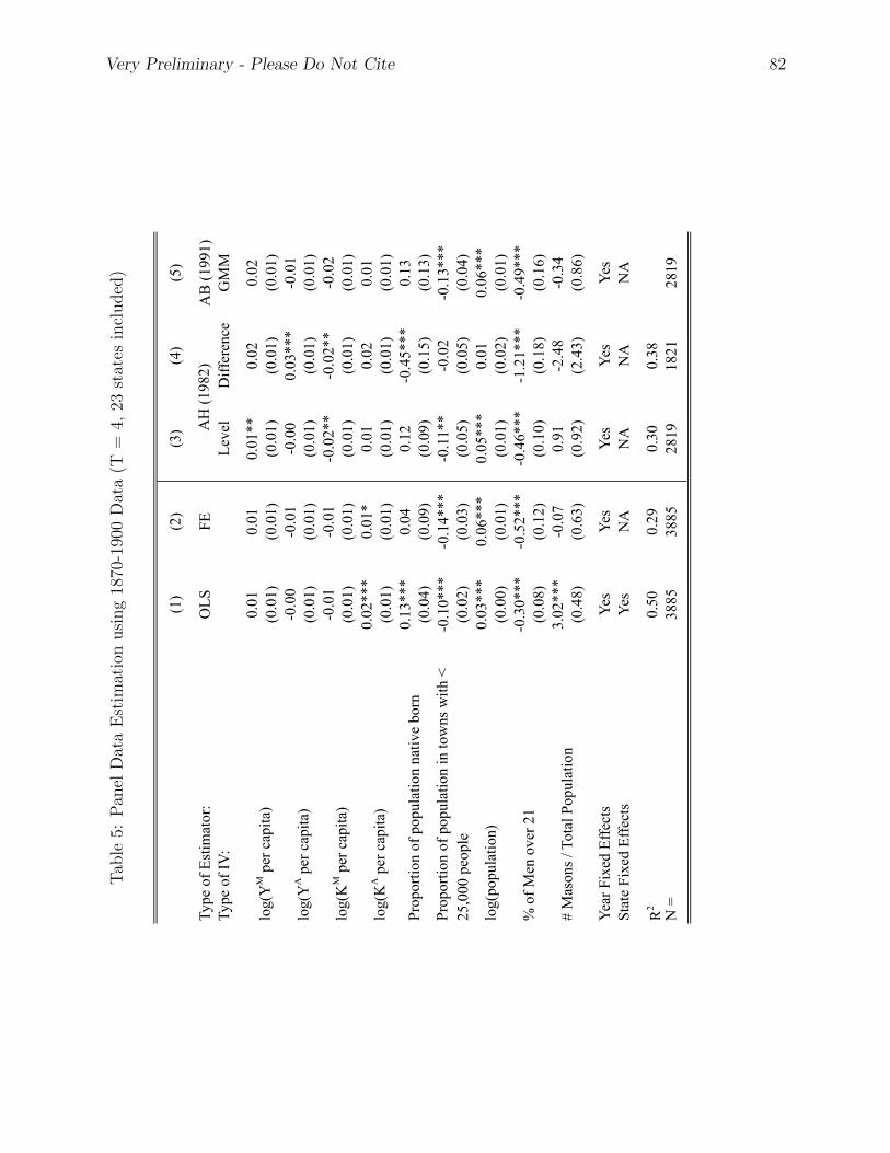
Very Preliminary - Please Do Not Cite 82
Tab
le5:
Pan
elD
ata
Est
imat
ion
usi
ng
1870
-190
0D
ata
(T=
4,23
stat
esin
cluded
)
(1)
(2)
(3)
(4)
(5)
Type
of E
stim
ator
:O
LSFE
AB
(199
1)Ty
pe o
f IV:
Leve
lD
iffer
ence
GM
M
0.01
0.01
0.01
**0.
020.
02(0
.01)
(0.0
1)(0
.01)
(0.0
1)(0
.01)
-0.0
0-0
.01
-0.0
00.
03**
*-0
.01
(0.0
1)(0
.01)
(0.0
1)(0
.01)
(0.0
1)-0
.01
-0.0
1-0
.02*
*-0
.02*
*-0
.02
(0.0
1)(0
.01)
(0.0
1)(0
.01)
(0.0
1)0.
02**
*0.
01*
0.01
0.02
0.01
(0.0
1)(0
.01)
(0.0
1)(0
.01)
(0.0
1)0.
13**
*0.
040.
12-0
.45*
**0.
13(0
.04)
(0.0
9)(0
.09)
(0.1
5)(0
.13)
-0.1
0***
-0.1
4***
-0.1
1**
-0.0
2-0
.13*
**(0
.02)
(0.0
3)(0
.05)
(0.0
5)(0
.04)
0.03
***
0.06
***
0.05
***
0.01
0.06
***
(0.0
0)(0
.01)
(0.0
1)(0
.02)
(0.0
1)-0
.30*
**-0
.52*
**-0
.46*
**-1
.21*
**-0
.49*
**(0
.08)
(0.1
2)(0
.10)
(0.1
8)(0
.16)
3.02
***
-0.0
70.
91-2
.48
-0.3
4(0
.48)
(0.6
3)(0
.92)
(2.4
3)(0
.86)
Year
Fix
ed E
ffect
sYe
sYe
sYe
sYe
sYe
sSt
ate
Fixe
d Ef
fect
sYe
sN
AN
AN
AN
A
R2
0.50
0.29
0.30
0.38
N =
38
8538
8528
1918
2128
19
AH
(198
2)
log(
YM
per
cap
ita)
log(
KM
per
cap
ita)
# M
ason
s / T
otal
Pop
ulat
ion
% o
f Men
ove
r 21
log(
YA p
er c
apita
)
log(
KA p
er c
apita
)
Prop
ortio
n of
pop
ulat
ion
nativ
e bo
rn
Prop
ortio
n of
pop
ulat
ion
in to
wns
with
<
25,0
00 p
eopl
e
log(
popu
latio
n)

Very Preliminary - Please Do Not Cite 83
Tab
le6:
Fre
emas
onry
and
Soci
alH
eter
ogen
eity
in18
70
(1)
(2)
(3)
(4)
(5)
(6)
(7)
(8)
(9)
0.03
**0.
02**
0.02
**0.
03*
0.03
*0.
000.
000.
010.
01(0
.01)
(0.0
1)(0
.01)
(0.0
2)(0
.02)
(0.0
3)(0
.03)
(0.0
3)(0
.03)
0.00
0.01
0.00
0.02
0.02
-0.0
4-0
.04
0.00
0.02
(0.0
1)(0
.01)
(0.0
1)(0
.02)
(0.0
2)(0
.04)
(0.0
4)(0
.03)
(0.0
3)0.
010.
000.
000.
00-0
.00
-0.0
00.
000.
07**
0.06
**(0
.01)
(0.0
1)(0
.01)
(0.0
2)(0
.02)
(0.0
2)(0
.02)
(0.0
3)(0
.03)
0.02
**0.
03**
0.03
***
0.03
**0.
03**
0.07
***
0.07
***
-0.0
5-0
.04
(0.0
1)(0
.01)
(0.0
1)(0
.01)
(0.0
1)(0
.02)
(0.0
2)(0
.04)
(0.0
4)0.
17**
0.13
*0.
20**
0.00
0.10
0.18
*0.
33**
0.38
**0.
46**
(0.0
7)(0
.07)
(0.0
8)(0
.08)
(0.1
0)(0
.11)
(0.1
5)(0
.19)
(0.2
0)-0
.00
0.04
0.04
0.02
0.04
(0.0
9)(0
.08)
(0.0
8)(0
.10)
(0.1
0)0.
03**
*0.
02**
*0.
02**
*0.
02*
0.02
*0.
020.
010.
020.
02(0
.01)
(0.0
1)(0
.01)
(0.0
1)(0
.01)
(0.0
2)(0
.02)
(0.0
2)(0
.02)
-0.0
7-0
.07
-0.0
8-0
.47*
*-0
.50*
*0.
130.
070.
290.
29(0
.12)
(0.1
2)(0
.12)
(0.2
0)(0
.20)
(0.2
0)(0
.19)
(0.2
3)(0
.24)
3.77
***
10.4
7***
4.01
***
19.9
6***
3.22
**14
.54*
*2.
0314
.47*
*(0
.75)
(2.7
2)(0
.93)
(6.3
1)(1
.48)
(7.0
1)(1
.76)
(6.3
9)-8
.62*
*-1
8.28
**-1
4.69
-19.
67**
(3.4
9)(7
.12)
(9.0
1)(9
.70)
R2
0.59
0.61
0.61
0.62
0.62
0.66
0.66
0.44
0.46
N =
10
1210
1210
1266
066
023
123
112
112
1
log(
YM p
er c
apita
)
log(
YA p
er c
apita
)
log(
KM p
er c
apita
)
log(
KA p
er c
apita
)
> 66
%Sh
are
of O
utpu
t fro
m M
anuf
actu
ring
# M
ason
s / T
otal
Pop
ulat
ion
(% M
ason
s) X
(% N
ativ
e)
< 33
%34
-66%
Prop
ortio
n of
pop
ulat
ion
nativ
e bo
rn
Prop
ortio
n of
pop
ulat
ion
in to
wns
with
< 2
5,00
0 pe
ople
log(
popu
latio
n)
% o
f Men
ove
r 21

Very Preliminary - Please Do Not Cite 84
Tab
le7:
Eth
nic
Hom
ogen
eity
and
Fre
emas
onry
-P
anel
Dat
aE
stim
ates
(1)
(2)
(3)
(4)
(5)
(6)
(7)
(8)
(9)
(10)
(11)
(12)
0.01
0.01
0.01
0.00
-0.0
0-0
.00
0.01
0.01
0.01
0.01
0.01
0.01
(0.0
1)(0
.01)
(0.0
1)(0
.01)
(0.0
1)(0
.01)
(0.0
1)(0
.01)
(0.0
1)(0
.01)
(0.0
1)(0
.01)
-0.0
0-0
.00
-0.0
0-0
.01
-0.0
1-0
.01
(0.0
1)(0
.01)
(0.0
1)(0
.01)
(0.0
1)(0
.01)
-0.0
0-0
.00
-0.0
00.
000.
000.
00-0
.01
-0.0
1-0
.01
-0.0
1-0
.01
-0.0
1(0
.01)
(0.0
1)(0
.01)
(0.0
1)(0
.01)
(0.0
1)(0
.01)
(0.0
1)(0
.01)
(0.0
1)(0
.01)
(0.0
1)0.
02**
*0.
02**
*0.
02**
*0.
02**
0.01
**0.
01*
0.02
***
0.02
***
0.02
***
0.01
*0.
01*
0.01
**(0
.01)
(0.0
1)(0
.01)
(0.0
1)(0
.01)
(0.0
1)(0
.01)
(0.0
1)(0
.01)
(0.0
1)(0
.01)
(0.0
1)0.
06*
0.04
0.09
**-0
.07
-0.0
60.
030.
16**
*0.
12**
*0.
20**
*0.
040.
040.
13(0
.03)
(0.0
3)(0
.04)
(0.0
5)(0
.05)
(0.0
6)(0
.04)
(0.0
4)(0
.04)
(0.0
9)(0
.09)
(0.0
9)-0
.06*
*-0
.06*
*-0
.06*
*-0
.13*
**-0
.12*
**-0
.11*
**-0
.11*
**-0
.10*
**-0
.10*
**-0
.14*
**-0
.14*
**-0
.13*
**(0
.03)
(0.0
3)(0
.03)
(0.0
4)(0
.03)
(0.0
3)(0
.02)
(0.0
2)(0
.02)
(0.0
3)(0
.03)
(0.0
3)0.
02**
*0.
02**
*0.
02**
*0.
04**
*0.
04**
*0.
04**
*0.
03**
*0.
03**
*0.
02**
*0.
06**
*0.
06**
*0.
05**
*(0
.00)
(0.0
0)(0
.00)
(0.0
1)(0
.01)
(0.0
1)(0
.00)
(0.0
0)(0
.00)
(0.0
1)(0
.01)
(0.0
1)-0
.45*
**-0
.48*
**-0
.49*
**-0
.75*
**-0
.73*
**-0
.75*
**-0
.28*
**-0
.30*
**-0
.31*
**-0
.52*
**-0
.52*
**-0
.59*
**(0
.09)
(0.0
9)(0
.09)
(0.1
3)(0
.13)
(0.1
3)(0
.08)
(0.0
8)(0
.08)
(0.1
2)(0
.12)
(0.1
2)3.
98**
*9.
65**
*2.
05**
14.3
6***
3.51
***
11.7
4***
0.02
17.9
2***
(0.5
3)(2
.97)
(0.9
2)(4
.30)
(0.5
1)(2
.20)
(0.7
8)(3
.92)
-6.7
8**
-14.
60**
*-1
0.18
***
-21.
87**
*(3
.39)
(4.9
4)(2
.56)
(4.6
1)R
20.
450.
460.
460.
230.
230.
240.
490.
500.
500.
290.
290.
30N
=
3818
3818
3818
3818
3818
3818
3885
3885
3885
3885
3885
3885
Pool
ed O
LS
log(
KA p
er c
apita
)
log(
YA p
er c
apita
)
log(
KM
per
cap
ita)
OLS
FE
# M
ason
s / T
otal
Pop
ulat
ion
(% M
ason
s) X
(% N
ativ
e)
1860
-190
0 Pa
nel D
ata
1870
-190
0 Pa
nel D
ata
Prop
ortio
n of
pop
ulat
ion
in to
wns
with
<
25,0
00 p
eopl
e
Prop
ortio
n of
pop
ulat
ion
nativ
e bo
rn
log(
popu
latio
n)
% o
f Men
ove
r 21
FE
log(
YM
per
cap
ita)

Very Preliminary - Please Do Not Cite 85
Tab
le8:
Eth
nic
Fra
ctio
nal
izat
ion
-P
anel
Dat
aE
stim
ates
(1)
(2)
(3)
(4)
(5)
(6)
(7)
(8)
(9)
(10)
(11)
(12)
(13)
(14)
0.02
*0.
02**
0.02
*0.
02**
0.02
**0.
02*
0.02
**0.
010.
010.
010.
010.
010.
010.
02(0
.01)
(0.0
1)(0
.01)
(0.0
1)(0
.01)
(0.0
1)(0
.01)
(0.0
1)(0
.01)
(0.0
1)(0
.01)
(0.0
1)(0
.01)
(0.0
1)0.
000.
00-0
.00
-0.0
00.
000.
000.
00-0
.01*
-0.0
1-0
.01
-0.0
1*-0
.01*
-0.0
1*-0
.01*
(0.0
1)(0
.01)
(0.0
1)(0
.01)
(0.0
1)(0
.01)
(0.0
1)(0
.01)
(0.0
1)(0
.01)
(0.0
1)(0
.01)
(0.0
1)(0
.01)
-0.0
1-0
.02
-0.0
2*-0
.02*
-0.0
2*-0
.02*
-0.0
2*-0
.01
-0.0
1-0
.01
-0.0
1-0
.01
-0.0
1-0
.01
(0.0
1)(0
.01)
(0.0
1)(0
.01)
(0.0
1)(0
.01)
(0.0
1)(0
.01)
(0.0
1)(0
.01)
(0.0
1)(0
.01)
(0.0
1)(0
.01)
0.01
***
0.02
***
0.02
***
0.02
***
0.01
***
0.02
***
0.02
***
0.02
***
0.02
***
0.02
***
0.02
***
0.02
***
0.02
***
0.02
***
(0.0
1)(0
.01)
(0.0
1)(0
.01)
(0.0
1)(0
.01)
(0.0
1)(0
.01)
(0.0
1)(0
.01)
(0.0
1)(0
.01)
(0.0
1)(0
.01)
-0.1
3***
-0.1
2***
-0.1
0***
-0.1
0***
-0.1
3***
-0.1
1***
-0.1
0***
-0.1
6***
-0.1
5***
-0.1
5***
-0.1
3***
-0.1
5***
-0.1
5***
-0.1
3***
(0.0
3)(0
.03)
(0.0
2)(0
.02)
(0.0
3)(0
.02)
(0.0
2)(0
.04)
(0.0
4)(0
.04)
(0.0
4)(0
.04)
(0.0
4)(0
.04)
0.03
***
0.03
***
0.03
***
0.03
***
0.03
***
0.03
***
0.03
***
0.06
***
0.07
***
0.07
***
0.06
***
0.06
***
0.06
***
0.06
***
(0.0
0)(0
.00)
(0.0
0)(0
.00)
(0.0
0)(0
.00)
(0.0
0)(0
.01)
(0.0
1)(0
.01)
(0.0
1)(0
.01)
(0.0
1)(0
.01)
-0.2
3***
-0.2
8***
-0.3
1***
-0.3
3***
-0.3
1***
-0.3
2***
-0.3
2***
-0.5
1***
-0.5
3***
-0.5
3***
-0.6
1***
-0.5
2***
-0.5
2***
-0.5
4***
(0.0
8)(0
.09)
(0.0
9)(0
.09)
(0.0
8)(0
.08)
(0.0
8)(0
.11)
(0.1
1)(0
.11)
(0.1
2)(0
.10)
(0.1
0)(0
.10)
0.17
***
0.02
(0.0
4)(0
.09)
0.09
*0.
050.
12**
0.04
0.04
0.14
(0.0
5)(0
.05)
(0.0
6)(0
.09)
(0.0
9)(0
.09)
-0.0
4-0
.06
-0.0
5-0
.18
-0.1
8-0
.11
(0.0
9)(0
.09)
(0.1
0)(0
.11)
(0.1
1)(0
.12)
3.86
***
11.2
7***
4.06
***
1.61
*0.
2818
.66*
**0.
25-6
.86*
**(0
.51)
(2.6
2)(0
.50)
(0.9
6)(0
.81)
(3.8
6)(0
.82)
(1.7
2)-9
.87*
**-2
3.45
***
(2.7
3)(4
.52)
-6.2
3-1
7.72
**(5
.48)
(8.0
2)-0
.04*
*-0
.03
-0.0
9***
-0.0
1-0
.01
-0.1
2(0
.02)
(0.0
2)(0
.03)
(0.0
7)(0
.07)
(0.0
7)5.
32**
*16
.19*
**(1
.74)
(3.2
1)R
20.
470.
480.
490.
490.
470.
490.
490.
320.
330.
330.
340.
320.
320.
34N
=
2931
2931
2931
2931
2931
2931
2931
2931
2931
2931
2931
2931
2931
2931
(% M
ason
s) X
(% F
orei
gn P
aren
tage
)
EFI
(% M
ason
s) X
(EFI
)
Prop
ortio
n of
pop
ulat
ion
nativ
e bo
rn, n
ativ
e pa
rent
age
Prop
ortio
n of
pop
ulat
ion
nativ
e bo
rn, a
t le
ast o
ne fo
reig
n pa
rent
# M
ason
s / T
otal
Pop
ulat
ion
(% M
ason
s) X
(% N
ativ
e Pa
rent
age)
Prop
ortio
n of
pop
ulat
ion
in to
wns
with
<
25,0
00 p
eopl
elo
g(po
pula
tion)
% o
f Men
ove
r 21
% N
ativ
e B
orn
log(
YM
per
cap
ita)
log(
YA p
er c
apita
)
log(
KM
per
cap
ita)
log(
KA p
er c
apita
)
Pool
ed O
LSFi
xed
Effe
cts
*:
Sig
nifi
can
ceat
10%
level
,**:
Sig
nifi
cant
at
5%
level
,***:
Sig
nifi
can
ceat
the
1%
level
.

Very Preliminary - Please Do Not Cite 86
Tab
le9:
Rel
igio
us
Hom
ogen
eity
and
Fre
emas
onry
-P
anel
Dat
aE
stim
ates
(1)
(2)
(3)
(4)
(5)
(6)
(7)
(8)
(9)
(10)
(11)
(12)
(13)
(14)
(15)
0.01
0.01
0.00
-0.0
00.
000.
000.
020.
000.
000.
00-0
.00
0.00
-0.0
0-0
.00
-0.0
0(0
.01)
(0.0
1)(0
.01)
(0.0
1)(0
.01)
(0.0
1)(0
.01)
(0.0
1)(0
.01)
(0.0
1)(0
.01)
(0.0
2)(0
.01)
(0.0
1)(0
.01)
-0.0
0-0
.01
-0.0
00.
00-0
.00
-0.0
0-0
.02
-0.0
0-0
.00
0.00
0.00
0.00
0.00
0.00
0.00
(0.0
1)(0
.01)
(0.0
1)(0
.01)
(0.0
1)(0
.01)
(0.0
1)(0
.01)
(0.0
1)(0
.01)
(0.0
1)(0
.02)
(0.0
1)(0
.01)
(0.0
1)0.
03**
*0.
02**
*0.
03**
*0.
03**
*0.
03**
*0.
03**
*0.
03**
*0.
03**
*0.
03**
*0.
03**
*0.
03**
*0.
02**
*0.
03**
*0.
03**
0.03
**(0
.01)
(0.0
1)(0
.01)
(0.0
1)(0
.01)
(0.0
1)(0
.01)
(0.0
1)(0
.01)
(0.0
1)(0
.01)
(0.0
1)(0
.01)
(0.0
1)(0
.01)
-0.0
8**
-0.1
0**
-0.0
7-0
.04
-0.0
4-0
.21*
**-0
.14*
*-0
.15*
**-0
.13*
*-0
.12*
*-0
.16*
**0.
12-0
.11
-0.1
0-0
.12*
(0.0
4)(0
.05)
(0.0
4)(0
.05)
(0.0
5)(0
.04)
(0.0
6)(0
.05)
(0.0
5)(0
.05)
(0.0
5)(0
.16)
(0.0
6)(0
.06)
(0.0
7)0.
03**
*0.
03**
*0.
03**
*0.
01**
0.01
**0.
09**
*0.
07**
*0.
09**
*0.
07**
*0.
07**
*0.
11**
*0.
09**
*0.
11**
*0.
10**
*0.
10**
*(0
.01)
(0.0
1)(0
.01)
(0.0
1)(0
.01)
(0.0
1)(0
.01)
(0.0
1)(0
.01)
(0.0
1)(0
.01)
(0.0
2)(0
.01)
(0.0
2)(0
.02)
-0.2
2**
-0.2
8***
-0.2
1*-0
.18
-0.1
9-0
.55*
**-0
.47*
**-0
.56*
**-0
.65*
**-0
.65*
**-0
.75*
**-0
.51*
**-0
.76*
**-0
.83*
**-0
.79*
**(0
.11)
(0.1
1)(0
.11)
(0.1
4)(0
.14)
(0.1
3)(0
.13)
(0.1
3)(0
.17)
(0.1
7)(0
.22)
(0.1
8)(0
.22)
(0.2
4)(0
.24)
2.50
***
2.20
***
2.39
***
2.25
***
1.17
-0.0
30.
27-0
.32
-0.3
20.
952.
52**
1.63
2.25
*1.
910.
59(0
.89)
(0.8
2)(0
.88)
(0.8
5)(0
.77)
(0.9
7)(1
.03)
(0.9
7)(0
.98)
(1.0
5)(1
.21)
(1.3
1)(1
.21)
(1.3
3)(1
.11)
-0.1
7***
-0.0
90.
06(0
.06)
(0.0
6)(0
.04)
-3.0
9-1
.44
-1.5
7-1
.60
-6.6
3*-6
.05*
-6.1
6*-5
.69*
-12.
56-5
.11
-5.4
0-6
.27*
(2.9
2)(2
.84)
(2.8
7)(2
.87)
(3.6
1)(3
.25)
(3.2
4)(3
.20)
(8.1
7)(3
.89)
(3.8
4)(3
.79)
0.04
**0.
020.
010.
010.
04**
0.03
**0.
03*
0.03
*-0
.01
0.04
*0.
04*
0.04
*(0
.02)
(0.0
1)(0
.01)
(0.0
1)(0
.02)
(0.0
1)(0
.02)
(0.0
2)(0
.03)
(0.0
2)(0
.02)
(0.0
2)0.
10**
*0.
08**
*0.
030.
050.
02-0
.03
(0.0
3)(0
.03)
(0.0
3)(0
.04)
(0.0
5)(0
.06)
2.54
*-3
.30*
8.11
*(1
.49)
(2.0
0)(4
.48)
R2
0.56
0.57
0.56
0.55
0.55
0.49
0.55
0.49
0.38
0.39
N =
17
2812
7317
2816
5016
5017
2812
7317
2816
5016
5011
8336
311
8311
1911
19
Pool
ed O
LSFi
xed
Effe
cts
AB
(199
1)
log(
YM
per
cap
ita)
log(
KM
per
cap
ita)
log(
KA p
er c
apita
)Pr
opor
tion
of p
opul
atio
n in
tow
ns w
ith <
25
,000
peo
ple
log(
popu
latio
n)
% o
f Men
ove
r 21
# M
ason
s per
cap
ita
# C
atho
lic se
ats p
er c
apita
# Je
wis
h se
ats p
er c
apita
# se
ats i
n al
l chu
rche
s per
cap
ita
RFI
(RFI
) X (#
Mas
ons p
er c
apita
)
*:
Sig
nifi
can
ceat
10%
level
,**:
Sig
nifi
cant
at
5%
level
,***:
Sig
nifi
can
ceat
the
1%
level
.
AB
(1991)
inst
rum
ents
for
both
Fre
emaso
ns
per
cap
ita
an
dth
ein
tera
ctof
Fre
emaso
ns
per
cap
ita
wit
hR
FI.

Very Preliminary - Please Do Not Cite 87
Tab
le10
:F
reem
ason
ryan
dE
duca
tion
alE
xp
endit
ure
sin
the
Mid
-19t
hC
entu
ry(1
850)
`
(1)
(2)
(3)
(4)
(5)
(6)
(7)
(8)
0.00
**0.
00**
-0.0
0**
-0.0
0**
0.00
0.00
0.00
0.00
(0.0
0)(0
.00)
(0.0
0)(0
.00)
(0.0
2)(0
.02)
(0.0
1)(0
.01)
-0.0
0**
-0.0
0**
0.00
**0.
00**
-0.0
0-0
.00
0.00
0.00
(0.0
0)(0
.00)
(0.0
0)(0
.00)
(0.0
2)(0
.02)
(0.0
1)(0
.01)
0.00
***
0.00
***
0.00
-0.0
00.
01**
*0.
01**
*0.
000.
00(0
.00)
(0.0
0)(0
.00)
(0.0
0)(0
.00)
(0.0
0)(0
.00)
(0.0
0)0.
000.
00-0
.00*
**-0
.00*
**-0
.13
-0.1
4*0.
020.
02(0
.00)
(0.0
0)(0
.00)
(0.0
0)(0
.08)
(0.0
8)(0
.09)
(0.0
9)-0
.00
-0.0
00.
000.
000.
150.
140.
010.
00(0
.00)
(0.0
0)(0
.00)
(0.0
0)(0
.23)
(0.2
3)(0
.10)
(0.1
0)0.
00*
0.00
*-0
.00
-0.0
00.
01**
0.01
**0.
010.
01(0
.00)
(0.0
0)(0
.00)
(0.0
0)(0
.01)
(0.0
1)(0
.01)
(0.0
1)-0
.00
-0.0
00.
00-0
.00
0.02
0.01
-0.0
6-0
.07
(0.0
0)(0
.00)
(0.0
0)(0
.00)
(0.1
0)(0
.10)
(0.0
6)(0
.06)
-0.0
50.
13**
*1.
732.
01(0
.07)
(0.0
5)(3
.06)
(2.1
7)R
20.
360.
360.
420.
450.
220.
220.
060.
06N
=
482
482
482
482
482
482
482
482
log(
YM
per
cap
ita)
log(
KM
per
cap
ita)
log(
KA p
er c
apita
)Pr
opor
tion
of p
opul
atio
n in
tow
ns w
ith <
2,5
00
peop
lePr
opor
tion
of p
opul
atio
n in
tow
ns w
ith 2
,500
-25
,000
peo
ple
log(
popu
latio
n)
% o
f Men
ove
r 21
# M
ason
s / T
otal
Pop
ulat
ion
Publ
icPr
ivat
e (A
cade
my)
Taxa
tion
# Te
ache
rs p
er P
oten
tial S
tude
nt1
Publ
ic E
duca
tion
Inco
me
from
Publ
ic F
unds
Not
es:
[1]:
Ap
oten
tial
studen
tis
ever
yone
bet
wee
nth
eag
esof
5-19
.C
han
ging
this
toth
eto
tal
pop
ula
tion
only
affec
tsth
e
size
ofth
ep
oint
esti
mat
es.
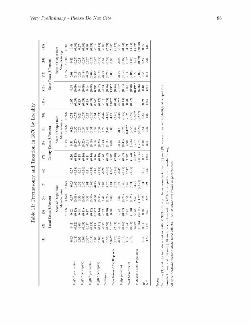
Very Preliminary - Please Do Not Cite 88
Tab
le11
:F
reem
ason
ryan
dT
axat
ion
in18
70by
Loca
lity
(1)
(2)
(3)
(4)
(5)
(6)
(7)
(8)
(9)
(10)
(11)
(12)
(13)
(14)
(15)
< 33
%33
-66%
> 66
%<
33 %
33-6
6%>
66%
< 33
%33
-66%
> 66
%
-0.0
5-0
.11
0.02
-0.6
7-0
.05
0.27
0.20
0.51
-0.2
30.
74-0
.05
-0.0
90.
08-0
.43
-0.4
8(0
.11)
(0.1
2)(0
.13)
(0.8
8)(0
.62)
(0.1
8)(0
.18)
(0.2
7)(0
.55)
(0.7
7)(0
.09)
(0.0
9)(0
.11)
(0.2
7)(0
.40)
0.02
-0.0
00.
040.
300.
320.
210.
180.
070.
24-0
.21
0.13
0.11
0.29
0.23
0.27
(0.0
9)(0
.09)
(0.1
1)(0
.81)
(0.4
5)(0
.16)
(0.1
6)(0
.22)
(0.5
4)(0
.77)
(0.0
9)(0
.09)
(0.1
9)(0
.29)
(0.4
0)0.
32*
0.31
*0.
170.
510.
010.
110.
11-0
.21
0.47
0.12
0.15
0.14
-0.0
90.
25*
0.40
(0.1
4)(0
.13)
(0.1
2)(0
.50)
(0.6
2)(0
.14)
(0.1
4)(0
.19)
(0.3
1)(0
.51)
(0.0
8)(0
.08)
(0.0
9)(0
.12)
(0.2
9)0.
070.
130.
38**
-0.0
0-0
.75
0.10
0.16
0.16
0.39
0.04
0.26
*0.
29*
0.36
*0.
38*
-0.1
9(0
.09)
(0.1
1)(0
.14)
(0.3
3)(0
.47)
(0.1
9)(0
.19)
(0.2
5)(0
.34)
(0.7
3)(0
.12)
(0.1
2)(0
.17)
(0.1
8)(0
.43)
-0.2
1-0
.55
-0.2
31.
493.
02-0
.28
-0.6
3-1
.43
2.79
-0.4
4-0
.17
-0.3
4-0
.93
0.68
-0.8
9(0
.55)
(0.5
0)(0
.70)
(1.2
2)(4
.26)
(0.8
0)(0
.82)
(1.1
1)(1
.48)
(4.6
0)(0
.53)
(0.5
6)(0
.72)
(0.5
9)(2
.59)
5.84
**6.
13**
0.00
0.00
2.81
4.99
*5.
30*
0.00
0.00
4.17
3.03
**3.
19**
0.00
0.00
2.88
*(2
.26)
(2.3
3).
.(3
.24)
(2.4
6)(2
.40)
..
(2.4
6)(0
.84)
(0.8
4).
.(1
.17)
-0.1
3-0
.16
-0.4
30.
040.
24-0
.45
-0.5
0-0
.46
-0.2
1-0
.40
-0.2
5*-0
.28*
-0.2
5-0
.05
-0.3
3(0
.15)
(0.1
6)(0
.32)
(0.2
2)(0
.40)
(0.2
7)(0
.27)
(0.4
3)(0
.26)
(0.4
7)(0
.13)
(0.1
3)(0
.19)
(0.0
9)(0
.24)
1.17
1.24
2.92
1.56
6.49
3.51
*3.
60*
4.90
8.42
**-3
.25
0.98
1.02
2.14
2.12
*-1
.21
(0.7
2)(0
.73)
(1.5
0)(1
.25)
(5.2
1)(1
.77)
(1.7
4)(3
.66)
(2.5
5)(5
.57)
(0.9
2)(0
.90)
(2.0
6)(1
.06)
(3.2
3)34
.99
59.6
66.
6734
.25
36.8
3**
17.1
64.
4272
.58*
*18
.49*
*8.
777.
2743
.39*
(21.
86)
(50.
18)
(11.
93)
(23.
78)
(11.
14)
(17.
70)
(20.
50)
(22.
37)
(6.8
6)(7
.02)
(10.
89)
(20.
50)
R2
0.32
0.33
0.38
0.26
0.31
0.36
0.37
0.30
0.51
0.65
0.39
0.40
0.38
0.59
0.65
N =
11
7311
7374
729
712
912
4712
4780
329
814
612
4712
4780
329
814
6
Stat
e Ta
xes (
$/Pe
rson
)
Shar
e of
Out
put f
rom
M
anuf
actu
ring
Shar
e of
Out
put f
rom
M
anuf
actu
ring
Shar
e of
Out
put f
rom
M
anuf
actu
ring
Loca
l Tax
es ($
/Per
son)
Cou
nty
Taxe
s ($/
Pers
on)
# M
ason
s / T
otal
Pop
ulat
ion
% o
f Men
ove
r 21
log(
YM
per
cap
ita)
log(
YA p
er c
apita
)
log(
KM
per
cap
ita)
log(
KA p
er c
apita
)
% N
ativ
e
% in
Tow
ns <
25,
000
peop
le
log(
popu
latio
n)
Note
s:
Colu
mn
s(3
)an
d(8
)in
clu
de
cou
nti
esw
ith≤
33%
of
ou
tpu
tfr
om
manu
fact
uri
ng,
(4)
an
d(9
)are
cou
nti
esw
ith
34-6
6%
of
ou
tpu
tfr
om
manu
fact
uri
ng
an
d(5
)an
d(1
0)
incl
ud
eco
unti
esw
ith≥
67%
of
ou
tpu
tfr
om
manu
fact
uri
ng.
All
spec
ifica
tion
sin
clu
de
state
fixed
effec
ts.
Rob
ust
stan
dard
erro
rsin
pare
nth
eses
.
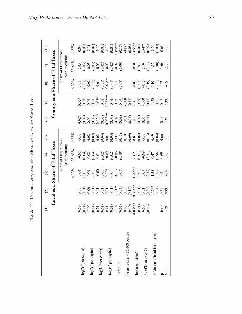
Very Preliminary - Please Do Not Cite 89
Tab
le12
:F
reem
ason
ryan
dth
eShar
eof
Loca
lto
Sta
teT
axes
(1)
(2)
(3)
(4)
(5)
(6)
(7)
(8)
(9)
(10)
< 33
%33
-66%
> 66
%<
33%
33-6
6%>
66%
0.00
0.00
0.00
-0.0
3-0
.00
0.02
*0.
02*
0.01
0.05
0.04
(0.0
1)(0
.01)
(0.0
1)(0
.04)
(0.0
4)(0
.01)
(0.0
1)(0
.01)
(0.0
3)(0
.03)
-0.0
0-0
.00
0.00
0.02
0.02
0.01
0.01
-0.0
2-0
.03
-0.0
1(0
.01)
(0.0
1)(0
.01)
(0.0
4)(0
.02)
(0.0
1)(0
.01)
(0.0
2)(0
.03)
(0.0
2)0.
010.
01-0
.00
0.01
0.02
-0.0
2**
-0.0
2*-0
.01
-0.0
2-0
.02
(0.0
1)(0
.01)
(0.0
1)(0
.02)
(0.0
4)(0
.01)
(0.0
1)(0
.01)
(0.0
2)(0
.03)
0.01
0.01
0.02
*-0
.00
0.01
-0.0
3***
-0.0
3***
-0.0
3**
-0.0
3-0
.02
(0.0
1)(0
.01)
(0.0
1)(0
.02)
(0.0
3)(0
.01)
(0.0
1)(0
.01)
(0.0
2)(0
.03)
-0.0
9-0
.10*
-0.1
3-0
.06
-0.1
90.
020.
030.
01-0
.07
0.65
***
(0.0
5)(0
.05)
(0.0
8)(0
.10)
(0.1
3)(0
.06)
(0.0
6)(0
.08)
(0.0
9)(0
.17)
0.08
0.09
0.10
-0.0
8-0
.08
-0.1
4*(0
.10)
(0.1
0)(0
.09)
(0.1
1)(0
.11)
(0.0
8)0.
03**
*0.
03**
*0.
03**
*0.
020.
01-0
.01
-0.0
1-0
.01
-0.0
10.
05**
*(0
.01)
(0.0
1)(0
.01)
(0.0
1)(0
.02)
(0.0
1)(0
.01)
(0.0
1)(0
.01)
(0.0
1)0.
000.
010.
05-0
.09
-0.0
00.
00-0
.00
-0.1
50.
100.
54**
(0.0
6)(0
.06)
(0.1
5)(0
.11)
(0.1
3)(0
.11)
(0.1
1)(0
.19)
(0.1
1)(0
.22)
1.12
**1.
330.
470.
49-0
.73
0.10
-1.3
5-0
.50
(0.5
4)(0
.85)
(0.9
6)(0
.84)
(0.5
8)(0
.85)
(0.9
8)(1
.00)
R2
0.69
0.69
0.71
0.69
0.66
0.46
0.46
0.42
0.60
0.63
N =
93
993
961
622
895
939
939
616
228
95
log(
YM p
er c
apita
)
Shar
e of
Out
put f
rom
M
anuf
actu
ring
Shar
e of
Out
put f
rom
M
anuf
actu
ring
Loc
al a
s a
Shar
e of
Tot
al T
axes
Cou
nty
as a
Sha
re o
f Tot
al T
axes
log(
YA p
er c
apita
)
log(
KM p
er c
apita
)
log(
KA p
er c
apita
)
# M
ason
s / T
otal
Pop
ulat
ion
% N
ativ
e
% in
Tow
ns <
25,
000
peop
le
log(
popu
latio
n)
% o
f Men
ove
r 21

Very Preliminary - Please Do Not Cite 90
Tab
le13
:C
orre
late
sof
Fre
emas
onry
duri
ng
the
19th
Cen
tury
(1)
(2)
(3)
(4)
(5)
(6)
(8)
(9)
(10)
(11)
1850
1860
1870
1880
1890
1900
1850
1860
1870
1890
-0.0
5-0
.01
0.00
-0.0
5-0
.01
0.09
-0.0
20.
03-0
.04
0.01
(0.0
5)(0
.04)
(0.0
6)(0
.05)
(0.0
5)(0
.06)
(0.0
3)(0
.04)
(0.0
6)(0
.05)
-0.0
30.
07**
-0.0
70.
38**
*0.
02-0
.02
0.08
0.00
(0.0
3)(0
.03)
(0.1
2)(0
.06)
(0.0
3)(0
.05)
(0.0
7)(0
.05)
0.05
0.03
0.06
0.10
*0.
020.
020.
01-0
.12
(0.0
5)(0
.04)
(0.0
7)(0
.05)
(0.0
5)(0
.06)
(0.0
6)(0
.11)
0.04
*0.
04**
-0.0
2-0
.06*
0.03
-0.3
3***
0.07
***
0.04
-0.0
70.
06(0
.02)
(0.0
2)(0
.03)
(0.0
3)(0
.13)
(0.0
6)(0
.03)
(0.0
6)(0
.05)
(0.1
3)0.
270.
66**
*0.
67**
*1.
12**
*1.
30**
*0.
020.
80**
0.98
***
(0.1
7)(0
.25)
(0.2
4)(0
.24)
(0.3
1)(0
.26)
(0.3
6)(0
.26)
-0.2
3**
-0.0
5-0
.63*
**-0
.32*
*-0
.24
0.07
-0.4
7***
0.27
-0.1
7-0
.07
(0.1
1)(0
.16)
(0.2
1)(0
.16)
(0.1
7)(0
.15)
(0.0
7)(0
.25)
(0.2
5)(0
.16)
0.06
**0.
12**
*0.
16**
*0.
11**
*-0
.06
-0.1
8***
0.07
**-0
.07
0.01
-0.1
2***
(0.0
3)(0
.03)
(0.0
3)(0
.02)
(0.0
4)(0
.05)
(0.0
3)(0
.06)
(0.0
6)(0
.04)
0.56
0.63
0.23
0.31
0.87
2.84
***
0.68
2.33
***
2.16
*1.
25**
(0.4
0)(0
.48)
(0.5
7)(0
.33)
(0.5
8)(0
.70)
(0.4
7)(0
.89)
(1.3
0)(0
.63)
-0.0
6-1
.22*
**-0
.33
(0.0
8)(0
.39)
(0.3
9)65
.90*
**-0
.80
-9.9
8**
-9.0
5**
(24.
04)
(12.
28)
(4.4
7)(3
.86)
0.06
*0.
37**
*0.
32**
*0.
26**
*(0
.03)
(0.1
4)(0
.12)
(0.0
9)0.
23**
*0.
61**
*0.
48**
0.45
*(0
.08)
(0.1
8)(0
.20)
(0.2
4)R
20.
270.
330.
260.
22N
=
392
576
839
1279
# C
atho
lic s
eats
per
cap
ita
# Je
wis
h se
ats
per c
apita
# se
ats
in a
ll ch
urch
es p
er c
apita
Rel
igio
us F
ract
iona
lizat
ion
Prop
ortio
n of
pop
ulat
ion
nativ
e bo
rnPr
opor
tion
of p
opul
atio
n in
tow
ns
with
< 2
5,00
0 pe
ople
log(
popu
latio
n)
% o
f Men
ove
r 21
log(
YM
per
cap
ita)
log(
YA p
er c
apita
)
log(
KM
per
cap
ita)
log(
KA p
er c
apita
)

Very Preliminary - Please Do Not Cite 91
Tab
le14
:D
eter
min
ants
of19
thC
entu
ryF
reem
ason
ry:
Pan
elD
ata
Anal
ysi
s
(1)
(2)
(3)
(4)
(5)
(6)
(7)
(8)
Year
s of D
ata:
1850
-190
018
60-1
900
1870
-190
018
50-1
900
1860
-190
018
70-1
900
1850
-189
018
60-1
890
0.03
0.02
0.00
0.03
0.04
*0.
020.
020.
01(0
.03)
(0.0
3)(0
.03)
(0.0
3)(0
.02)
(0.0
3)(0
.04)
(0.0
3)0.
07**
*0.
06**
*(0
.03)
(0.0
2)-0
.02
0.00
0.03
-0.0
3-0
.03
-0.0
0-0
.02
-0.0
1(0
.03)
(0.0
3)(0
.03)
(0.0
3)(0
.02)
(0.0
3)(0
.04)
(0.0
3)0.
06**
*0.
06**
*-0
.06*
*0.
12**
*0.
10**
*-0
.01
0.18
***
0.13
***
(0.0
2)(0
.01)
(0.0
2)(0
.04)
(0.0
2)(0
.02)
(0.0
6)(0
.05)
0.44
***
1.03
***
-0.5
4***
0.31
-0.8
6**
(0.0
9)(0
.12)
(0.1
3)(0
.23)
(0.4
0)-0
.12
-0.2
7***
-0.4
6***
-0.9
4-0
.52*
**-0
.61*
**-0
.73
0.15
(0.1
1)(0
.08)
(0.0
9)(0
.59)
(0.1
0)(0
.10)
(0.5
6)(0
.17)
-0.0
00.
08**
*0.
11**
*-0
.17
-0.0
30.
09**
*-0
.31*
-0.4
9***
(0.0
4)(0
.02)
(0.0
2)(0
.11)
(0.0
2)(0
.02)
(0.1
6)(0
.12)
0.90
**0.
540.
63*
-0.1
5-0
.57
-0.2
5-0
.19
-0.3
8(0
.41)
(0.3
3)(0
.33)
(0.6
0)(0
.39)
(0.3
7)(0
.54)
(1.4
0)-4
8.41
-5.6
4(3
2.65
)(7
.88)
0.04
0.11
(0.0
6)(0
.10)
0.15
0.09
(0.1
1)(0
.13)
R2
0.37
0.23
0.24
0.47
0.20
0.09
0.47
0.37
N =
25
5239
0939
2325
5239
0939
2316
5012
71
# se
ats i
n al
l chu
rche
s per
cap
ita
Rel
igio
us F
ract
iona
lizat
ion
log(
YM
per
cap
ita)
log(
YA p
er c
apita
)
log(
KM
per
cap
ita)
log(
KA p
er c
apita
)
Prop
ortio
n of
pop
ulat
ion
nativ
e bo
rn
Prop
ortio
n of
pop
ulat
ion
in to
wns
with
<
25,0
00 p
eopl
e
log(
popu
latio
n)
% o
f Men
ove
r 21
# Je
wis
h se
ats p
er c
apita
Pool
ed O
LS E
stim
ates
Fixe
d Ef
fect
Est
imat
es
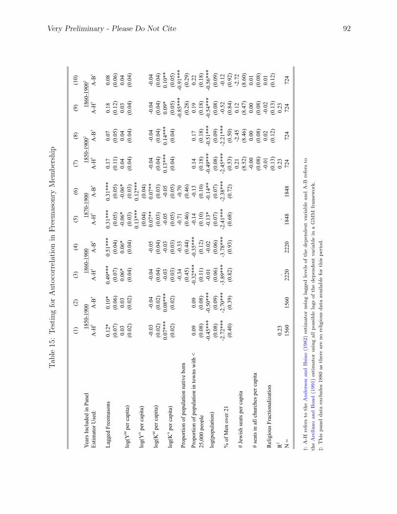
Very Preliminary - Please Do Not Cite 92
Tab
le15
:T
esti
ng
for
Auto
corr
elat
ion
inF
reem
ason
ryM
emb
ersh
ip
(1)
(2)
(3)
(4)
(5)
(6)
(7)
(8)
(9)
(10)
Year
s Inc
lude
d in
Pan
elEs
timat
or U
sed:
A-H
†A
-B†
A-H
†A
-B†
A-H
†A
-B†
A-H
†A
-B†
A-H
†A
-B†
Lagg
ed F
reem
ason
s0.
12*
0.10
*0.
49**
*0.
51**
*0.
31**
*0.
31**
*0.
170.
070.
180.
08(0
.07)
(0.0
6)(0
.07)
(0.0
4)(0
.05)
(0.0
5)(0
.11)
(0.0
5)(0
.12)
(0.0
6)0.
030.
030.
06*
0.06
*-0
.06*
-0.0
6*0.
040.
040.
030.
04(0
.02)
(0.0
2)(0
.04)
(0.0
4)(0
.03)
(0.0
3)(0
.04)
(0.0
4)(0
.04)
(0.0
4)0.
13**
*0.
12**
*(0
.04)
(0.0
4)-0
.03
-0.0
4-0
.04
-0.0
50.
07**
0.07
**-0
.04
-0.0
4-0
.04
-0.0
4(0
.02)
(0.0
2)(0
.04)
(0.0
4)(0
.03)
(0.0
3)(0
.04)
(0.0
4)(0
.04)
(0.0
4)0.
07**
*0.
08**
*-0
.03
-0.0
3-0
.05
-0.0
50.
13**
*0.
14**
*0.
09*
0.10
**(0
.02)
(0.0
2)(0
.03)
(0.0
3)(0
.05)
(0.0
5)(0
.04)
(0.0
4)(0
.05)
(0.0
5)-0
.34
-0.3
3-0
.71
-0.7
0-0
.85*
**-0
.91*
**(0
.45)
(0.4
4)(0
.46)
(0.4
6)(0
.28)
(0.2
9)0.
090.
09-0
.32*
**-0
.35*
**-0
.14
-0.1
30.
140.
170.
190.
22(0
.08)
(0.0
8)(0
.11)
(0.1
2)(0
.10)
(0.1
0)(0
.18)
(0.1
8)(0
.18)
(0.1
8)-0
.45*
**-0
.50*
**-0
.01
-0.0
2-0
.13*
-0.1
4**
-0.4
9***
-0.5
1***
-0.5
4***
-0.5
6***
(0.0
8)(0
.09)
(0.0
6)(0
.06)
(0.0
7)(0
.07)
(0.0
8)(0
.09)
(0.0
8)(0
.09)
-2.7
2***
-2.7
0***
-3.8
9***
-3.7
8***
-2.4
1***
-2.3
8***
-2.4
5***
-2.2
1***
-0.5
2-0
.12
(0.4
0)(0
.39)
(0.8
2)(0
.93)
(0.6
8)(0
.72)
(0.5
3)(0
.50)
(0.8
4)(0
.92)
0.21
-2.4
50.
12-2
.72
(8.5
2)(8
.46)
(8.4
7)(8
.60)
-0.0
00.
000.
000.
01(0
.08)
(0.0
8)(0
.08)
(0.0
8)-0
.01
0.02
-0.0
20.
01(0
.13)
(0.1
2)(0
.13)
(0.1
2)R
20.
23.
.0.
230.
23N
=
1560
1560
2220
2220
1848
1848
724
724
724
724
log(
YM
per
cap
ita)
log(
YA p
er c
apita
)
log(
KM
per
cap
ita)
1850
-190
018
60-1
900
# Je
wis
h se
ats p
er c
apita
# se
ats i
n al
l chu
rche
s per
cap
ita
Rel
igio
us F
ract
iona
lizat
ion
log(
KA p
er c
apita
)
Prop
ortio
n of
pop
ulat
ion
nativ
e bo
rn
Prop
ortio
n of
pop
ulat
ion
in to
wns
with
<
25,0
00 p
eopl
e
log(
popu
latio
n)
1870
-190
018
50-1
900‡
1860
-190
0‡
% o
f Men
ove
r 21
†:A
-Hre
fers
toth
eA
nd
erso
nan
dH
siao
(1982)
esti
mato
ru
sin
gla
gged
level
sof
the
dep
end
ent
vari
ab
lean
dA
-Bre
fers
to
the
Are
llan
oan
dB
on
d(1
991)
esti
mato
ru
sin
gall
poss
ible
lags
of
the
dep
end
ent
vari
ab
lein
aG
MM
fram
ework
.
‡:T
his
pan
eld
ata
excl
ud
es1880
as
ther
eare
no
reli
gio
us
data
availab
lefo
rth
isp
erio
d.

Very Preliminary - Please Do Not Cite 93
Tab
le16
:F
reem
ason
ryan
dE
nro
llm
ent
inth
eM
id-1
9th
Cen
tury
(185
0)
(1)
(2)
(3)
(4)
(5)
(6)
0.01
0.01
0.04
**0.
04**
-0.0
1-0
.01
(0.0
1)(0
.01)
(0.0
2)(0
.02)
(0.0
0)(0
.00)
-0.0
1-0
.01
-0.0
4**
-0.0
4**
0.01
*0.
01(0
.01)
(0.0
1)(0
.02)
(0.0
2)(0
.00)
(0.0
0)0.
02**
*0.
02**
*0.
02**
*0.
02**
*0.
00-0
.00
(0.0
1)(0
.01)
(0.0
0)(0
.01)
(0.0
0)(0
.00)
0.06
0.06
0.12
0.12
-0.0
8***
-0.0
9***
(0.1
3)(0
.13)
(0.0
8)(0
.08)
(0.0
3)(0
.03)
0.04
0.03
0.02
0.01
0.04
0.03
(0.1
4)(0
.14)
(0.1
0)(0
.10)
(0.0
5)(0
.05)
0.04
***
0.04
***
0.05
***
0.05
***
-0.0
0-0
.00
(0.0
1)(0
.01)
(0.0
1)(0
.01)
(0.0
0)(0
.00)
-0.2
4*-0
.26*
-0.1
5-0
.16
-0.0
1-0
.01
(0.1
3)(0
.13)
(0.1
3)(0
.13)
(0.0
8)(0
.08)
2.49
2.28
1.35
(1.6
7)(2
.29)
(0.9
9)R
20.
560.
560.
350.
350.
340.
35N
=
482
482
482
482
482
482
% o
f Men
ove
r 21
log(
KA p
er c
apita
)
Prop
ortio
n of
pop
ulat
ion
in to
wns
with
2,5
00-2
5,00
0 pe
ople
Prop
ortio
n of
pop
ulat
ion
in to
wns
with
< 2
,500
peo
ple
log(
popu
latio
n)
# M
ason
s / T
otal
Pop
ulat
ion
Enro
llmen
t Am
ong
Men
and
Wom
en A
ges
5-19
log(
YM
per
cap
ita)
log(
KM
per
cap
ita)
Tota
lPu
blic
Priv
ate