how did the keiretsu system solve the hold-up problem in
TRANSCRIPT

How did the keiretsu system solve the hold-up problem in the Japanese
automobile industry?
by
Sota Ichiba
Thesis submitted in partial fulfillment of the
requirements for the Degree of
Bachelor of Arts with
Honours in Economics
Acadia University
June, 2015
© Copyright by Sota Ichiba, 2015

ii
This thesis by Sota Ichiba
is accepted in its present form by the
Department of Economics
as satisfying the thesis requirements for the degree of
Bachelor of Arts with Honours
Approved by the Thesis Supervisor
__________________________ ____________________
Dr. Xiaoting Wang Date
Approved by the Head of the Department
__________________________ ____________________
Dr. Brian VanBlarcom Date
Approved by the Honours Committee
__________________________ ____________________
Dr. Anthony Thompson Date
iii
I, Sota Ichiba, grant permission to the University Librarian at Acadia
University to reproduce, loan ordistribute copies of my thesis in
microform, paper or electronic formats on a non-profit basis. I, however,
retain the copyright in my thesis.
_________________________________
Signature of Author
_________________________________
Date

iv
Acknowledgements
I would like to thank my supervisor, Dr. Wang Xiaoting for her
tremendous effort to help me getting through the process, and Dr. Hassouna
Moussa for his continuous support since I entered to this university. I also
would like to thank Dr. Andrew Davis who helped me to improve my thesis.
Finally, I would like to give my sincere gratitude to my family for their
emotional and financial support. I would have not been able to finish the
thesis without their helps.

v
Contents
Abstract .................................................................................................................... viii
1. Introduction .......................................................................................................... 1
1.1 Statement of the problem .................................................................................. 1
1.2 Introduction of the hold-up problem ................................................................. 2
1.3 A case study of the hold-up problem: GM-Fisher Body ..................................... 3
1.4 Modifications of the hold-up model ................................................................... 4
2. Background of the Japanese keiretsu system ..................................................... 6
2.1 History and characteristics of the keiretsu system .......................................... 6
2.2 An example of the keiretsu relationship: Toyota-Denso ................................... 9
2.3 Adapting the hold-up model to the keiretsu system ....................................... 11
3. The model ........................................................................................................... 12
3.1 Setup of the game ............................................................................................ 12
3.2 Decentralized equilibrium ............................................................................... 18
3.3 Outside option .................................................................................................. 19
3.4 Repeated game equilibrium ............................................................................. 24
4. Extension to the model ....................................................................................... 30
4.1 Setup of the game ............................................................................................ 30

vi
4.2 Equilibrium ..................................................................................................... 34
5. Conclusion .......................................................................................................... 35
Reference ................................................................................................................... 37

vii
Figures and Propositions
Figure 1 The structure of the subgame ...........................................................17
Proposition 1: ....................................................................................................23
Proposition 2: ....................................................................................................27

viii
Abstract
The Japanese car industry enjoyed a steady expansion path from 1960,
following the keiretsu system, the Japanese style of non-vertically integrated
system. This is a result of the dissolution of the zaibatsu and is characterized by
less internalization and flexible contracts. Other characteristics of the keiretsu
include that the buyer of the product can buy the same product from another
different keiretsu company, as seen in the Toyota-Denso relationship. The model
proposed by this thesis incorporates these additions to the classical hold-up
model, proposed by Grossman and Hart (1986) to examine the efficiency of such
system. In particular, the buyer now has an option to partially buy the same
product from another company. This introduces implicit competition within the
system as seen in the keiretsu relationship. Using backward induction to
establish a subgame perfect Nash equilibrium, I derive a result indicating that
efficiency improves from the classic case of a complete non-vertically integrated
system when the buyer has high bargaining power over the share of surplus,
and that the magnitude of competition within the keiretsu relationship does not
affect efficiency, measured by the amount of underinvestment. I also propose a
possible extension to the model to further relax the assumption in the model.
1
1. Introduction
1.1 Statement of the problem
The Japanese economy expanded enormously in the past 50 years. In
particular, the automobile industry grew steadily over the past few decades and
became one of the biggest in the world. The Japanese car industry has a
different structure from its American counterparts. This system, called the
keiretsu system, is characterized by a non-vertically integrated model with a
strong bond among the companies in the supply chain. For example, the part
suppliers to Toyota, the largest car company in Japan, openly share any
problems in production and try to improve quality collectively even though they
are not direct subsidiaries of Toyota. This seems counterintuitive since a
non-vertically integrated model is a source of what are called hold-up
inefficiencies. However, several assumptions of the hold-up model, such as the
absence of other sellers, are not met in the keiretsu system.
This thesis attempts to examine the efficiency of the Japanese car
industry from the perspective of the hold-up problem by relaxing the
assumptions in the original hold-up model, primarily by the introduction of
implicit competition among supply firms. This is done by extending the repeated

2
hold-up model by Castaneda (2004) to allow an outside company which supplies
the same product to the buyer. The result of a subgame perfect Nash equilibrium
in the model suggests that the efficiency of the system is independent from the
level of competition as long as there is some, and keiretsu improves efficiency
only if the parent company has large bargaining power in the allocation of
surplus within the system.
1.2 Introduction of the hold-up problem
The hold-up problem is one of the most heavily studied topics in
economics because it connects the study of incentives to the study of the
boundaries of firms. It occurs when the seller is protected by an exclusive
contract, which ensures that a certain amount of their product is bought by the
buyer, and the investment is relation-specific. Relation specific investment (RSI)
refers to investment that has no use outside of the relationship. This problem
causes inefficiencies from the seller’s underinvestment. This inefficiency only
happens in a non-vertically integrated system since the downstream firm is able
to dictate the upstream firm’s action in the case of a vertical integrated system.
In his cost-benefit analysis of vertical mergers, Williamson (1979) finds that in a

3
transaction cost economy, the cost of production in a non-vertically integrated
model might exceed that of vertically integrated firms because of the associated
cooperation cost. Grossman and Hart (1986) took a different approach to this
problem by using the idea of an imperfect contract. They stated that in a
non-vertically integrated model, it is practically impossible to write a complete
contract that protects both firms from all events that would occur in the future.
As a result, the upstream firm becomes reluctant to invest in relation-specific
assets since the return on such investment is insufficient to justify the optimal
investment which maximizes efficiency of the whole system, and the upstream
firm is not able to confirm the future commitment from the downstream firm.
1.3 A case study of the hold-up problem: GM-Fisher Body
A consequence of such contracts can be found in the GM-Fisher Body
relationship. Fisher Body and GM signed a long term exclusive dealing contract
in order to protect their relation-specific assets in 1919. Soon after that, in the
early 1920s, Fisher Body started to extort extra investment from GM by
refusing to build a new factory near GM’s factory. GM had no choice but to agree
to this demand because they could not void the contract and they did not have
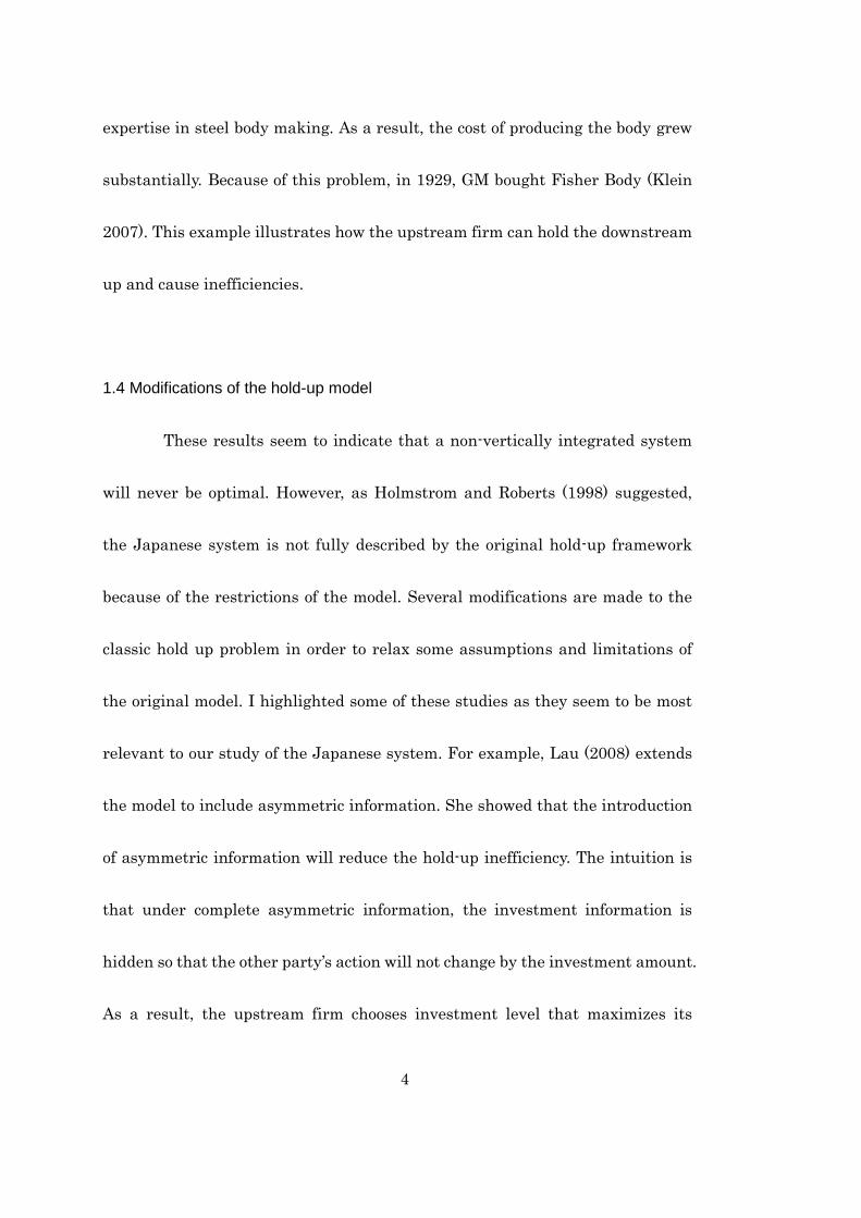
4
expertise in steel body making. As a result, the cost of producing the body grew
substantially. Because of this problem, in 1929, GM bought Fisher Body (Klein
2007). This example illustrates how the upstream firm can hold the downstream
up and cause inefficiencies.
1.4 Modifications of the hold-up model
These results seem to indicate that a non-vertically integrated system
will never be optimal. However, as Holmstrom and Roberts (1998) suggested,
the Japanese system is not fully described by the original hold-up framework
because of the restrictions of the model. Several modifications are made to the
classic hold up problem in order to relax some assumptions and limitations of
the original model. I highlighted some of these studies as they seem to be most
relevant to our study of the Japanese system. For example, Lau (2008) extends
the model to include asymmetric information. She showed that the introduction
of asymmetric information will reduce the hold-up inefficiency. The intuition is
that under complete asymmetric information, the investment information is
hidden so that the other party’s action will not change by the investment amount.
As a result, the upstream firm chooses investment level that maximizes its

5
return without considering the upstream firm’s reaction, which leads to the
optimal level of investment. Castaneda (2004) proved that in a repeated
relationship with the possibility of terminating the contract and moving to
vertical integration, as the limit of the contract period goes to zero, both parties
act optimally and downstream buyer does not choose to integrate its upstream
supplier. Intuitively, this model eliminates the inefficiency by giving the
downstream company a threat strategy of vertical integration. This forces the
upstream company to invest optimally given that the duration of exclusive
contract is short. In another study, Schmidt and Nöldeke (1998) showed that the
hold-up inefficiencies will be eliminated if the investment is done sequentially.
The main assumption of the paper is that the upstream firm’s profit depends on
how much the downstream values the upstream firm after the first investment
by the upstream firm is carried out. Investment now has two types of returns;
the return from the lower cost of production, and the return from being valued
more by the downstream firm. Consequently, the investment becomes more
lucrative to the upstream firm, encouraging them to invest optimally.
The model proposed by this thesis is built to reflect the Japanese
keiretsu relationship. In particular, implicit competitions within the system as

6
well as repeated game dynamics, which are main characteristics of the Japanese
non-vertically integrated system, are incorporated into the model. This model
allows us to examine the efficiency of non-vertically integrated firms with
various outside options. A subgame perfect Nash equilibrium of the game
suggests that the keiretsu system improves efficiency from the complete
vertically integrated system only when the downstream firm has high
bargaining power in splitting the surplus made within the system.
The structure of the Japanese automobile industry is crucial to
understand the setup and implications of the model. In the next section, I will
discuss the Japanese system in depth. In section 3, the detailed model is
discussed. In chapter 4, I propose an extension of the model. Finally, I conclude
the paper in chapter 5.
2. Background of the Japanese keiretsu system
2.1 History and characteristics of the keiretsu system
The expansion of the Japanese automobile industry is a protracted
mystery for economists since the industry followed a different direction from its
competitors in other parts of the world. Nevertheless, the industry has

7
experienced a huge expansion. Toyota more than tripled its sales from 1960 to
1990 while US car manufacturers, such as Chrysler, reached a plateau in 1960
and did not grow since then (Toyota 2011 and Chrysler 2009). Attempts have
been made in order to find a key to growth by gathering differences between the
Japanese automobile industry and its US counterparts. Several papers,
including the research done by Asanuma (1988) and Ahmadjian and Lincoln
(1997) reached a similar conclusion that the Japanese car industry has lower
number of suppliers and the buyer-supplier relationship is closer in the
Japanese system compared to the United States. This is a result of the keiretsu
system which can be translated as “series” or “group”. The keiretsu system is
often understood as a type of structure specific to Japan. This is characterized
by a loosely tied group of companies. It is common in the automobile industry
where relation specific investment is frequently happening and the
manufacturer of the final product such as Toyota has to rely on many companies
in order to procure numerous parts required for production of car (Ito 2002).
This system was formed by a series of policies implemented in the post-war era
in Japan.
By the Allied Forces, the country underwent a major economic reform

8
after 1945 in order to demilitarize and recover the country. They called
dissolution of zaibatsu, a type of conglomerate formed in Japan. Zaibatsu is
described by a series of vertically integrated firms with a bank on top of the
structure. It was believed that by using its capital flow and economic influence
to the government, zaibatsu indirectly promoted totalitarianism and the war
(Noguchi 2008). The keiretsu system was born after the dissolution in order to
protect formerly the zaibatsu subsidiary companies and promote development of
these companies as a whole (Kikuchi 2011, Takada 2011). However, several
keiretsu including the Toyota keiretsu do not originate from zaibatsu. These are
purely made in order to facilitate information flow and production. The keiretsu
system has similarities to the zaibatsu structure as both systems are
characterized by a series of related firms albeit these differ in terms of
ownership of the whole system. Zaibatsu is directly and explicitly owned by a
single family whereas keiretsu is not. In fact, Nissan, the third largest car
manufacturer in Japan (Nissan 2014), used to be a part of a zaibatsu structure
named Nissan Konzern and later became loosely tied keiretsu called
Nissan-Hitachi group (Kikuchi 2011). On top of the keiretsu system, there is a
company called parent company that has its first-tier child companies which in

9
turn oversee companies in the next tier. For example, Toyota has several
first-tier companies like Denso and Aishin, supplying car electronics to Toyota
and then Denso has several second-tier companies such as Asmo which supplies
motors to Denso. However, there is no vertical integration prevalent in the
North American automobile industry because child companies are not directly
owned by its parent companies. In other words, they are financially independent
of each other. Moreover, keiretsu is not perfectly competitive as the child
companies are willing to share information within the system. For example, they
have extensive Supplier Networks and they jointly participate in research and
development process (Ku 2011).
2.2 An example of the keiretsu relationship: Toyota-Denso
One of the most prominent examples of the keiretsu relationship is the
Toyota-Denso partnership. Denso (Nihon Denso) is a spin-off company from
Toyota founded in 1949. As the translation of the company name suggests, it
makes car electronics. It is the largest car parts supplier in Japan and has
annual sales revenue of $40 billion (Fortune 2014). In her attempt to find the
source of the expansion of the Japanese car industry, Anderson (2003) studied

10
this relationship. She argues that Denso and Toyota are tied by a special
personal relationship. Denso originally was a part of Toyota until 1949 when the
company became unable to keep some of its direct subsidiary including the car
electronics section due to economic situation of the post-war Japan. When Denso
was founded, the president of Toyota, Kiichiro Toyoda, personally decided to lend
140 million Japanese Yen (14 million US Dollar) to Denso in hope of revitalizing
the struggling company. Denso never forgot this and paid back with their new
quality control system which became essential in Toyota’s success in the
automobile market. The relationship in reality is not as fixed as it seems to be.
Denso has an option to sell their product to other car companies. Meanwhile,
Toyota can buy from other supplier of the electronic parts. This is an example of
hostage model described in Williamson (1983) which promotes efficiency by
equalizing the bargaining power among the companies. Nevertheless, this
option is not prevalent in the system. For example, only 10% of the parts bought
by Nissan were from outside its keiretsu relationship (Asanuma 1988).
Anderson (2003) concluded that the history of good trust and the threat outside
options reduced opportunism and hence made them stick to the cooperative
equilibrium outcome of the game.

11
2.3 Adapting the hold-up model to the keiretsu system
By looking at the nature of the relationship, we see how it is different
from the previous models in the hold-up literatures. Firstly, the paper by
Grossman and Hart (1986) concludes that there is no way to avoid inefficiency if
the firms are not vertically integrated. The keiretsu system is not vertically
integrated yet seems to be efficient. Secondly, the information problem posed by
Lau’s model (2008) is not applicable to the relationship because the keiretsu
structure facilitates smooth flow of information by having many technological
meetings and joint research and development in order to reduce coordination
cost (Ku 2011). The sequential Investment model by Schmidt and Nöldeke
(1998) is not at least directly applicable here even though in the Toyota-Denso
case, there was an unofficial investment from Toyota since Toyota’s investment
is not meant to increase Denso’s willingness to be vertically integrated as it is
assumed in the paper. The repeated hold-up model with an option of vertical
integration by Castaneda (2004) provides a model similar to what previous
researchers described as the keiretsu structure. However, as Anderson (2003)
found out in the Toyota-Denso case, there is no option for Toyota to vertically

12
integrate Denso as its subsidiary because of a financial reason. Moreover,
production volume is not fixed when these companies sign a contract. These
factors were not included in the model of Castaneda (2004).
In order to better examine the efficiency of the Japanese model, this
thesis proposes a new model which incorporates the outside option given to the
buyer or the parent company as well as repeated nature of the relationship
based on Castaneda (2004).
3. The model
3.1 Setup of the game
We consider the simplest case in which there are two players, namely a
seller and a buyer. The buyer can buy the seller's product. In period 𝑡 ∈ ℕ, the
buyer values the seller's product at 𝑣(𝑞𝑡, 𝜃𝑡) where 𝑞𝑡 is the quantity and 𝜃𝑡 is
the state of the world variable, both at time t. The state of the world variable θ
takes any uncertainty, such as car demand and financial restriction, into
account. To make the problem simpler, 𝜃𝑡 is assumed to be independently and
identically distributed for any 𝑡 ∈ ℕ.

13
The cost of producing 𝑞𝑡 unit in the state of world θt is denoted as
𝑐1(𝑥, 𝑞𝑡, 𝜃𝑡) where x is the investment level undertaken by the seller. In
accordance to the existing hold-up literatures, the investment is assumed to be
completely relation specific. That is, the investment will remain unused outside
of the contract relationship. Investment is non-contractible which means the
investment amount cannot be specified in contracts. Therefore, the seller
determines the investment level so that the payoff for them is maximized.
The buyer has an outside option of purchasing the same product from
another inside company. However, the buyer must pay switching cost 𝑚 ∈ ℝ+
in order to do this. It follows that the total cost when the buyer chooses to obtain
the product from another company is 𝑐2(𝑥, 𝑞𝑡, 𝜃) + 𝑚 where c2 is the cost
structure for the outside company. This is a simplified assumption which allows
the buyer to buy the same product from another company.
To proceed, we need the following assumptions about property of the
functions;

14
For any θt ∈ Θ
1. 𝑣(⋅, 𝜃𝑡): ℝ+ → ℝ+ is continuously differentiable, increasing, and strictly
concave.
2. c1(⋅,⋅, θt): ℝ+ × ℝ+ → ℝ+ is continuously differentiable, decreasing in x,
increasing in q, and strictly convex.
Similarly to the model developed in Castaneda (2004), the game is
based on an extensive form. There is a contract period at the beginning followed
by the bargaining period. However, a modification is made in order to allow the
buyer to procure the product from another company. This indirectly introduces
competition to the relationship.
The structure of the game is as follows:
1. Contract Period. The buyer and the seller can bargain over the contract which
determines the form of the relationship. After the bargaining, the seller invests
x.
2. Each period t ∈ N has 4 sub-periods:

15
i. The buyer may be able to impose the allocation variable λ ∈ [0,1], the
fraction of total demand which she is going to buy from the seller in this
period. λ is an exogenous variable determined by factors such as
number of other firms supplying the same part to the buyer.
ii. Nature determines the state of the world θ.
iii. The buyer and the seller bargain the price for the trade which takes
place in this period. The seller decide the level of output 𝑞𝑡
iv. The seller produces the output and the payoff for the buyer and the
seller is realized.
After the state of the world is revealed to both parties, they negotiate
over the price and the quantity of the product. This bargaining process has the
following assumptions:
1. Efficiency: The bargaining process maximizes the surplus from the
trade taking place in the period subject to the earlier actions.

16
2. Alpha-Bargaining Solution: The result of the bargaining process in
period 2-iv always ensures that the buyer gains a fraction 0<𝛼<1 of the total
surplus from the trade.
3. Outside Option: The players always choose the outside option when
the payoff within the relationship is less than the outside option.
The parameter α can be thought of as relative bargaining power for the
seller. The higher α is, the higher the share of the surplus from the trade the
seller gets. It can be influenced by factors such as relative size and the financial
situation of the companies. Given the abstract nature of the model, however,
this variable is treated as an exogenous constant.
The newly added variable, λ, is meant to relax the model proposed by
Castaneda (2004). As we shall see, setting λ = 1 will duplicate the original
model by Grossman (1986) and λ = 0 corresponds to Castaneda (2004). Figure
1-1 shows visualization of the period 2.

17
Figure 1 The structure of the subgame
As in Grossman and Hart (1986), we assume that writing a complete
contract is impossible in practice, therefore, in this model, the contract 𝐶(𝑇, 𝑝)
consists of only 2 components. Once the parties sign a contract, a transfer which
amounts to T ∈ ℝ+ will be made from the buyer to seller in each period. The
variable p ∈ ℝ+ determines the period in which the buyer exclusively buys the
product from the seller. During the period, the buyer is unable to impose 𝜆
therefore the buyer must buy the full amount of the demand from the seller.
Let G(x), the present value of the total surplus within the relationship,
be.
G(x) = ∑ 𝛿𝑡
∞
𝑡=0
∫ 𝑣(𝑞∗(𝑥, 𝜃𝑡), 𝜃𝑡) − 𝑐1(𝑥, 𝑞∗(𝑥, 𝜃𝑡), 𝜃𝑡)𝑑𝐹𝜃
− 𝑥
where 𝑞∗(𝑥, 𝜃𝑡) = argmax 𝑣(𝑞∗, 𝜃𝑡) − 𝑐1(𝑥, 𝑞∗, 𝜃𝑡)

18
This is the present value of the stream of surplus within the system, subtracted
by the investment by the seller.
Since c1 is strictly convex by assumption, by using envelope theorem,
the optimal investment level x∗ is uniquely determined by the following
equation.
∑ 𝛿𝑡
∞
𝑡=0
∫𝛿𝑐1(𝑥∗, 𝑞𝑡(𝑥∗, 𝜃𝑡), 𝜃𝑡)
𝛿𝑥𝑑𝐹
𝜃
= −1 (1)
I examine whether the equilibrium in various setups result in
underinvestment for the seller which leads to inefficiency in the system.
3.2 Decentralized equilibrium
Firstly, we examine the case where the buyer and the seller agree to
sign an exclusive contract which prohibits the outside option for the seller for
the whole game. This case can be expressed as a contract C(T,∞) for an
arbitrary T ∈ ℝ+.
Lemma 1
For any contract C(T,∞), the present value of return for the buyer and

19
the seller in the relationship are
U𝑖B = 𝛼𝐺(𝑥) + 𝛼𝑥 − ∑ 𝛿𝑡
∞
𝑡=0
𝑇
U𝑖S = (1 − 𝛼)𝐺(𝑥) − 𝛼𝑥 + ∑ 𝛿𝑡
∞
𝑡=0
𝑇
Proof:
Assuming α-bargaining solution, for each period, the one period surplus
for the buyer and the seller are respectively
U𝑡B = 𝛼[𝑣(𝑞∗(𝑥, 𝜃𝑡), 𝜃𝑡) − 𝑐1(𝑥, 𝑞∗(𝑥, 𝜃𝑡), 𝜃𝑡)] − T
U𝑡S = (1 − 𝛼)[𝑣(𝑞∗(𝑥, 𝜃𝑡), 𝜃𝑡) − 𝑐1(𝑥, 𝑞∗(𝑥, 𝜃𝑡), 𝜃𝑡)] + T
Taking the present value of the stream of payoffs, including the cost of the
investment gives
U𝑖B = ∑ 𝛿𝑡
∞
𝑡=0
∫ U𝑡B𝑑𝐹 =
𝜃
𝛼𝐺(𝑥) + 𝛼𝑥 − ∑ 𝛿𝑡
∞
𝑡=0
(2)
U𝑖S = ∑ 𝛿𝑡
∞
𝑡=0
∫ U𝑡S𝑑𝐹 =
𝜃
(1 − 𝛼)𝐺(𝑥) − 𝛼𝑥 + ∑ 𝛿𝑡
∞
𝑡=0
𝑇 (3)
as desired. Q.E.D.
3.3 Outside option
Unlike the model by Castaneda (2004), the model proposed in the thesis
assumed the imperfect vertical integration outside option in lieu of the perfect
vertical integration option. In the keiretsu system, the buyer of the product can

20
implicitly introduce competition by exploiting the loose contract system
discussed in the paper of Asanuma (1988) and Ahmadjian and Lincoln (1997)
even though there is no direct competition in the system. If the seller performs
unsatisfactorily, the buyer can penalize such opportunistic behavior by imposing
λ in the later period and partly buy the product from another company.
Therefore, one can think of the fraction λ as a measure of competition inside the
keiretsu system. High λ indicates dependence on the seller for the particular
product. In the model, we assume λ to be an exogenous variable for simplicity
as quantifying this theoretical parameter can be hard. Moreover, to simplify the
model, we assume that the competitor company is a direct subsidiary of the
buyer and always invests optimally. This assumption might not hold in the
actual keiretsu relationship. Yet, without the assumption, it is hard to assume
another keiretsu company which invests optimally without any incentives. I let
H(x) = ∑ 𝛿𝑡
∞
𝑡=0
∫ 𝑣(𝑞𝑡(𝑥, 𝜃𝑡), 𝜃𝑡) − 𝑐2(𝑥, 𝑞𝑡(𝑥, 𝜃𝑡), 𝜃𝑡)𝑑𝐹𝜃
− 𝑥
be the total surplus function when the buyer buys the product from the outside
company where the cost function for the outside company c2 shares the same
property as c1. With these assumptions, the payoff for the outside option can be
defined.

21
Lemma 2
For any contract C(T,∞). The present value of return for the buyer and
the seller when the outside option was chosen are
𝑈𝑜𝐵 = λ (𝛼𝐺(𝑥) − ∑ 𝛿𝑡
∞
𝑡=1
𝑇) (1 + λ𝛼 − λ)𝑥 + (1 − λ)𝐻(𝑥∗) − 𝑀
𝑈𝑜𝑆 = λ ((1 − 𝛼)𝐺(𝑥) + ∑ 𝛿𝑡
∞
𝑡=1
𝑇) − (λ − 1 − λ𝛼)𝑥
Proof:
The one period payoff for the buyer and the seller are
U𝑡𝑜
B = λU𝑖B + (1 − λ)𝐻(𝑥∗) − 𝑀
U𝑖𝑜
S = λU𝑖S
By taking the present value of the sum of the payoff, we obtain the result.
Q.E.D.
The next lemma deals with the equilibrium investment level in a
non-vertically integrated model.
Lemma 3
For any contract C(T,∞), the equilibrium level of investment 𝑥𝐸 is
determined uniquely by

22
∑ 𝛿𝑡
∞
𝑡=0
∫𝛿𝑐1(𝑥∗, 𝑞𝑡(𝑥∗, 𝜃𝑡), 𝜃𝑡)
𝛿𝑥𝑑𝐹
𝜃
= −1 −𝛼
1 − 𝛼 (4)
Proof:
Since C(T,∞) is an exclusive contract for any future periods, the seller
only needs to maximize its own payoff without any restrictions. By invoking the
envelope theorem and differentiating U𝑖S in (3), we obtain
(1 − 𝛼)[∑ 𝛿𝑡
∞
𝑡=0
∫𝛿𝑐1(𝑥∗, 𝑞𝑡(𝑥∗, 𝜃𝑡), 𝜃𝑡)
𝛿𝑥𝑑𝐹 − 1] − 𝛼
𝜃
= 0 (5)
as the maximizing condition and the maximizer is unique since 𝑐1(𝑥, 𝑞𝑡(𝑥, 𝜃𝑡), 𝜃𝑡)
is strictly convex in x. Rearranging (5) gives the expression above. Q.E.D.
By contrasting the equilibrium investment level in (4) to the optimal
investment level given in (1), we can see that the seller underinvests by 𝛼
1−𝛼. The
alpha-bargaining process of dividing the total surplus distorts the seller’s
incentive to invest. The seller only obtains the fraction (1 − α) of the return of
investment compared to what it would have been in the vertically integrated
system hence becomes reluctant to invest. The result has exactly the same
implication as in the model of Grossman and Hart (1986) and Castaneda (2004).
Whether such an exclusive contract is implemented depends heavily on
the outside option for both the buyer and the seller. The contract implements

23
the relationship only if the payoff inside the relationship is larger than the
outside option for both the seller and the buyer. Since the model assumed that
only the buyer has access to the outside option, we only consider the condition
for the buyer.
Proposition 1
There exists a transfer T ∈ ℝ+ which implements the relationship if and
only if
G(xE) ≥ 𝐻(𝑥∗) − 𝑀
Proof:
The following condition must be satisfied in order for the buyer to fully
procure the product from the seller.
𝛼𝐺(𝑥𝐸) − (1 − 𝛼)𝑥𝐸 − ∑ 𝛿𝑡
∞
𝑡=0
𝑇 ≥ +𝐻(𝑥𝐸) −𝑀
1 − �̅�
(1 − 𝛼)𝐺(𝑥𝐸) − 𝛼𝑥𝐸 + ∑ 𝛿𝑡
∞
𝑡=0
𝑇 ≥ λ ((1 − 𝛼)𝐺(𝑥𝐸) + ∑ 𝛿𝑡
∞
𝑡=1
𝑇) − (λ − 1 − λ𝛼)𝑥𝐸
The second condition for the seller is always satisfied since λ ∈ [0,1]. Therefore,
there exists a transfer T ∈ ℝ+ if and only if the total surplus for the whole
system is larger than that of the outside option case. That is,
G(xE) ≥ λ𝐺(𝑥𝐸) + (1 − λ)𝐻(𝑥∗) − 𝑀

24
Rearranging this gives the desired expression. Q.E.D.
3.4 Repeated game equilibrium
Now, I allow p, the number of the exclusive contract period to be
different from infinity. The game becomes a repeated game between the seller
and buyer. At the end of each contract, the buyer can choose to impose λ on the
seller. With this setup, since seller always gets better payoff within the
relationship, the seller always wants to maintain the relationship. By using
backward induction, we can derive a subgame perfect Nash equilibrium.
Lemma 4
For contracts C(T,k) k ≠ ∞ , there exist a subgame perfect Nash
equilibrium in which the investment level, denoted as xE , is uniquely
determined by
∑ 𝛿𝑡
∞
𝑡=0
∫𝜕𝑐1(𝑥, 𝑞𝑡(𝑥∗, 𝜃𝑡), 𝜃𝑡)
𝜕𝑥𝑑𝐹
𝜃
= −1 −𝛼(1 − 𝛿𝑘) + 𝛿𝑘
1 − 𝛼(1 − 𝛿𝑘) (𝜆 ≠ 1) (6)
Proof:
The above analysis shows that in a sub game perfect equilibrium, after
the first contract, the buyer has to be indifferent between implementing the

25
relationship and imposing λ. The condition is written as
𝛼𝐺(𝑥𝐸(𝑘)) + 𝛼𝑥𝐸(𝑘) − ∑ 𝛿𝑡−𝑘
∞
𝑡=𝑘
𝑇𝑅
= 𝜆 (𝛼𝐺(𝑥𝐸(𝑘)) − ∑ 𝛿𝑡−𝑘
∞
𝑡=𝑘
𝑇𝑅) (1 + 𝜆𝛼 − 𝜆)𝑥𝐸(𝑘) + (1 − 𝜆)𝐻(𝑥∗) − 𝑀 (7)
where TR is renegotiated transfer after k periods.
The seller maximizes the payoff subject to the condition in (7).
max𝑥
(1 − 𝛼)𝐺(𝑥) − 𝛼𝑥 + ∑ 𝛿𝑡𝑇(𝑘) + ∑ 𝛿𝑇𝑅
∞
𝑡=𝑘
𝑘−1
𝑡=0
Assuming λ ≠ 0, the constraint (7) can be simplified to
αG(xE(𝑘, 𝜆)) − (1 − α)xE(𝑘, 𝜆) − ∑ 𝛿𝑡−𝑘𝑇𝑅
∞
𝑡=𝑘
= H(x∗) −M
1 − 𝜆 (8)
Substituting the constraint into the objective function yields
{1 − α(1 − δk)}G(x) − α(1 − δk)x − δkx + A where A = ∑ 𝛿𝑡𝑇(𝑘) − 𝛿𝑘{𝐻(𝑥∗) −𝑀
1 − 𝜆}
𝑘−1
𝑡=0
Optimizing the above function using envelope theorem leads to the desired
expression. Q.E.D.
Lemma 5
For contracts C(k,T) k ≠ ∞, the subgame perfect Nash equilibrium
investment level xE(𝑘, 𝜆) has the following properties;
1, 𝑑𝑥𝐸(𝑘, 𝜆)
𝑑𝑘< 0 (9)
2, 𝑑𝑥𝐸(𝑘, 𝜆)
𝑑𝛿> 0 (10)

26
3, Other than λ = 1, the value of λ will not change xE(𝑘, 𝜆).
Proof:
By construction, c(x) is strictly increasing and convex. Hence,
𝑑𝐺(𝑥)
𝑑𝑥< 0.
Therefore,
𝑑𝑥𝐸(𝑘, 𝜆)
𝑑𝑘=
𝑑𝑑𝑘
[𝛼(1 − 𝛿𝑘) + 𝛿𝑘
1 − 𝛼(1 − 𝛿𝑘)]
𝑑𝐺(𝑥)𝑑𝑥
< 0
Similarly,
𝑑𝑥𝐸(𝑘, 𝜆)
𝑑𝛿> 0 as
∂G
𝜕𝛿> 0
During the simplification process from (7) to (8), it was assumed that
λ ≠ 1. If λ = 1, then the solution becomes xE for any k since there is no option
for the buyer to change the allocation. If λ ≠ 1, the equilibrium investment is
xE(𝑘, 𝜆). Since xE(𝑘, 𝜆) does not have a term with λ, the investment level is
independent of λ.
Q.E.D.
This result of the comparative statics reflects the buyer’s penalization
strategy. When the contract period is long, one strategy for the seller is to
deviate from the optimal investment and let the buyer impose λ or offer lower
transfer after k periods. Whether this strategy gives better payoff for the seller
27
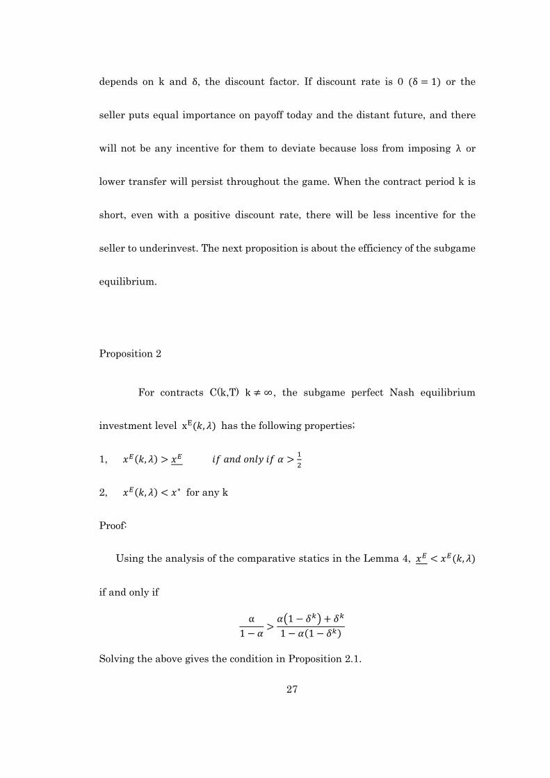
depends on k and δ, the discount factor. If discount rate is 0 (δ = 1) or the
seller puts equal importance on payoff today and the distant future, and there
will not be any incentive for them to deviate because loss from imposing λ or
lower transfer will persist throughout the game. When the contract period k is
short, even with a positive discount rate, there will be less incentive for the
seller to underinvest. The next proposition is about the efficiency of the subgame
equilibrium.
Proposition 2
For contracts C(k,T) k ≠ ∞, the subgame perfect Nash equilibrium
investment level xE(𝑘, 𝜆) has the following properties;
1, 𝑥𝐸(𝑘, 𝜆) > 𝑥𝐸 𝑖𝑓 𝑎𝑛𝑑 𝑜𝑛𝑙𝑦 𝑖𝑓 𝛼 >1
2
2, 𝑥𝐸(𝑘, 𝜆) < 𝑥∗ for any k
Proof:
Using the analysis of the comparative statics in the Lemma 4, 𝑥𝐸 < 𝑥𝐸(𝑘, 𝜆)
if and only if
α
1 − 𝛼>
𝛼(1 − 𝛿𝑘) + 𝛿𝑘
1 − 𝛼(1 − 𝛿𝑘)
Solving the above gives the condition in Proposition 2.1.

28
By (9) in the Lemma 5, the subgame perfect equilibrium investment level
xE(𝑘, 𝜆) reaches the maximum when k is approaching to 0. The investment level
evaluated at the point is
lim𝑘→0
∑ 𝛿𝑡
∞
𝑡=0
∫𝜕𝑐1(𝑥, 𝑞𝑡(𝑥∗, 𝜃𝑡), 𝜃𝑡)
𝜕𝑥𝑑𝐹
𝜃
= −1 −𝛼(1 − 𝛿𝑘) + 𝛿𝑘
1 − 𝛼(1 − 𝛿𝑘)
Comparing this to the social optimal investment, x∗, we have
lim𝑘→0
𝛼(1 − 𝛿𝑘) + 𝛿𝑘
1 − 𝛼(1 − 𝛿𝑘)= 1 > 0
Therefore, xE(𝑘, 𝜆) < 𝑥∗ for any k. Q.E.D.
The extended model has the same comparative statics as Castaneda
(2004). However, the equilibrium result indicates the opposite. In particular, on
the contrary to Castaneda (2004), the subgame perfect equilibrium investment
level is always less than the social optimal investment regardless of the
parameters. Moreover, this implies that the only condition needed for the buyer
to ensure the improved investment from the seller over the complete exclusive
contract situation is buyer’s high bargaining power even though introduction of
at least some competition is needed to avoid the case of complete exclusive
contract.
The result indicates that the amount of competition does not have any
effect on the equilibrium investment despite our intuitive belief that penalizing

29
opportunistic behaviors more enables the buyer to have more bargaining power
to make the seller invest optimally. This may be a result of the setup of the
model. Since the buyer only has two options, imposing λ or not, and the seller is
always worse off if the buyer chooses to impose λ, the seller always tries to avoid
such situations. Therefore, the value of λ becomes irrelevant from the seller’s
perspective.
Nevertheless, the efficiency condition in Proposition 2.1 makes sense in
the keiretsu relationship since in most of the keiretsu relationships, the parent
company is larger than the child company. Therefore we expect the parameter α
to be large. Furthermore, supply of some car parts is sometimes dominated by a
single company. For example, in 1992, about 75% of the demand for electronic
control unit (ECU) for fuel injection system by Toyota was supplied only through
Denso (Yunokami 2011). Although the share of demand does not directly
translate to the parameter λ, we can expect the value to be large.
Technically, the value of λ can be determined through finding a
subgame perfect Nash equilibrium for an extension to the 2 players model which
introduces the cost difference and internalization of λ . The model will be
discussed in the next chapter.

30
4. Extension to the model
4.1 Setup of the game
The extension to the model internalizes the determination of λ by
having two sellers that compete with each other. These companies differ in the
cost structure but have the same level of bargaining power over the surplus. The
setup relaxes the assumption made in the original model with a hypothetical
seller which always invests optimally. Moreover, this model allows the buyer to
freely choose λ at the end of each contract period. However, I introduce a
switching cost to penalize rapid movements in λ. Because of the nature of
multivariate optimization and the lack of functional form assumed in the model,
it is hard to obtain the closed form result for the game. Some implication can be
drawn from the model. The extended model may also give more implication
about λ which had almost no effect on the investment level in the original
model.
The cost for the first seller to produce 𝑞1𝑡 unit in the state of world θt
is denoted as 𝑐1(𝑥1, 𝑞1𝑡, 𝜃𝑡) where x1 is the investment level undertaken by the
seller one. Let 𝑐2(𝑥2, 𝑞2𝑡, 𝜃𝑡) be the cost function for the second seller.

31
Let the surplus function in the relationship between the buyer and seller 1 be
G(x1) = ∑ 𝛿𝑡
∞
𝑡=0
∫ 𝑣(𝑞1𝑡(𝑥1, 𝜃𝑡), 𝜃𝑡) − 𝑐1(𝑥1, 𝑞1𝑡
(𝑥1, 𝜃𝑡), 𝜃𝑡)𝑑𝐹𝜃
− 𝑥1
and the surplus in relation between the buyer and seller 2 be
H(x2) = ∑ 𝛿𝑡
∞
𝑡=0
∫ 𝑣(𝑞2𝑡(𝑥2, 𝜃𝑡), 𝜃𝑡) − 𝑐2(𝑥1, 𝑞2𝑡
(𝑥2, 𝜃𝑡), 𝜃𝑡)𝑑𝐹𝜃
− 𝑥2
We assume the following properties:
For any θt ∈ Θ
1. 𝑣(⋅, 𝜃𝑡): ℝ+ → ℝ+ is continuously differentiable, increasing, and strictly
concave.
2. c1(⋅,⋅, θt): ℝ+ × ℝ+ → ℝ+ is continuously differentiable, decreasing in x1,
increasing and linear in q1, and strictly convex in x1.
3. c2(⋅,⋅, θt): ℝ+ × ℝ+ → ℝ+ is continuously differentiable, decreasing in x2,
increasing and linear in q2, and strictly convex in x2.
The assumption changed from the original model by having linear cost
function. The cost function is strictly convex in investment so the optimal
investment level is uniquely determined.

32
The extended model has a similar structure to the original model.
However, the buyer now can set the allocation variable λ so that the payoff for
the buyer is maximized. Moreover, the buyer only determines total demand for
the good instead of individual demand.
The structure of the game is as follows:
1. Contract Period. The buyer and the sellers can bargain over the contract
which determines the form of the relationship. After the bargaining, the
seller i invests xi and the buyer determines the initial allocation λ0.
2. Each period t ∈ N has 4 sub-periods.
i. The buyer may change the allocation variable λ∈[0,1], the fraction of
total demand which she is going to buy from the seller 1 in this period.
However, she must incur the cost M(Δλ) where Δλ is the change in λ.
ii. Nature determines the state of the world θt.
iii. The buyer and the sellers bargain the price and quantity for the
trade in this period. The buyer decides the total demand Qt, not the
individual demand qi 𝑡 The output level for seller 1 qI𝑡 is determined

33
automatically by q1t = λQt. Similarly, the output level for the seller 2 is
q2𝑡 = (1 − λ)Qt.
iv. The sellers produce the output and the payoff for the buyer and the
sellers are realized.
To define the social optimal investment, I let K(λ) be the total surplus
in the system. Since G(x1) and H(x2) are linear, the function is defined by
K(λ, x1, 𝑥2) = λG(x1) + (1 − λ)H(x2)
The social optimal investment involves the Pareto optimal allocation
and it is obtained by maximizing K(λ, x1, 𝑥2). Due to the complexity of
multivariate optimization, the solution may not be a linear combination of (1)
similarly to the single seller case and the closed form solution may be hard to
obtain. If both sellers have access to the same technology, from a socially
optimal perspective, the choice of λ will not matter as products of seller 1 and
seller 2 are perfect substitutes. If one dominates the other in terms of the cost
structure, the value of λ that the buyer determines favors the seller with better
cost structure.

34
4.2 Equilibrium
Method of backward induction is used to solve for the subgame perfect
Nash equilibrium. For the first seller, they want to maximize the payoff
max𝑥
𝜆 ((1 − 𝛼)𝐺(𝑥𝑖) + ∑ 𝛿𝑡𝑘−1
𝑡=1
𝑇1 + ∑ 𝛿𝑇1𝑅
∞
𝑡=𝑘
) − (𝜆 − 1 − 𝜆𝛼)𝑥1
subject to the condition that the buyer will not choose allocation unfavorable to
them at the end of the first contract in time k. That is,
αK(λ0) + (𝜆0 − 1 − 𝜆0𝛼)𝑥1 + (−𝜆0 − (1 − 𝜆0)𝑎)𝑥2 + 𝜆0 ∑ 𝛿𝑡
𝑘−1
𝑡=1
𝑇1 + 𝜆0 ∑ 𝛿𝑡𝑇𝑅1
∞
𝑡=𝑘
+ (1 − λ0) ∑ 𝛿𝑡
𝑘−1
𝑡=0
𝑇2 + (1 − λ0) ∑ 𝛿𝑡𝑇𝑅2
∞
𝑡=𝑘
= αK(λ′) + (𝜆′ − 1 − 𝜆′𝛼)𝑥1 + (−𝜆′ − (1 − 𝜆′)𝑎)𝑥2 + 𝜆0 ∑ 𝛿𝑡
𝑘−1
𝑡=1
𝑇1 + 𝜆′ ∑ 𝛿𝑡𝑇𝑅1
∞
𝑡=𝑘
+ (1 − λ0) ∑ 𝛿𝑡
𝑘−1
𝑡=1
𝑇2 + (1
− λ′) ∑ 𝛿𝑡𝑇𝑅2
∞
𝑡=𝑘
− M(λ0 − λ) 𝑓𝑜𝑟 𝑎𝑛𝑦 λ < 𝜆0
The coefficients on x1 and x2 are derived similarly to the Lemma 1.
Since the buyer’s choice of λ depends on the sellers’ investment
decisions on x1 and x2, solving the constrained optimization problems gives a set
of best response function, x1∗(𝑥2), x2
∗(𝑥1). Therefore, solving the system of
equation gives the equilibrium decision of x1, x2, and λ. As the model does not

35
assume any functional form, similarly to the derivation of the social optimal, it
is hard to derive a closed-form solution to this. However, if we consider the
simplest case where c1 = 𝑐2 and M=0 for any λ, this model becomes similar to
the Bertrand model, and the optimal decision for the sellers is to invest
optimally since the buyer will always choose λ = 1 when x1 > 𝑥2 as c1(𝑥1, 𝑞) <
𝑐2(𝑥2, 𝑞) for any q and vice versa. If we introduce different technology and some
switching cost, working through the optimization becomes tedious. Moreover, it
is impossible to determine λ unless we assume some decision rule. This
extended model adds much more flexibility over the original model. Due to the
limitation of my background knowledge as well as the complexity of the model, I
will leave the analysis of the extended model in more general cases to future
research
5. Conclusion
This thesis attempts to improve the current hold-up models in order to
better describe the keiretsu system, the Japanese style of non-vertical
integrated model. This is done by adding an allocation variable λ to the
repeated hold-up model proposed by Castaneda (2004). The additions are meant

36
to capture characteristics of the keiretsu relationship, such as loose initial
contracts and repeated nature of the relationship, which are left uncaptured by
the original hold-up framework by Grossman and Hart (1986).
By solving for a subgame perfect Nash equilibrium for the model, it is
shown that the keiretsu style relationship is likely to improve efficiency of the
whole system, measured by the level of investment, when compared to a
complete non-vertical integration system without any outside option. The
efficiency condition found in the thesis does not involve the allocation variable λ,
which reflects the amount of competitiveness within the system. Contrary to the
findings of Castaneda (2004), the investment level is always less than the social
optimal level which maximizes the surplus among the upstream firms. The
model proposed by this thesis still has its limitations such as the exogeneity of λ
and, the hypothetical outside seller which invests optimally without any
incentives. To further examine the efficiency of the keiretsu system, my future
studies will focus on the internalization of the allocation variable, by introducing
strategic competition to the upstream sellers.

37
Reference
• Ahmadjian, C. L. and James R. Lincoln. 1997. Changing firm boundaries
in Japanese auto parts supply networks Center on Japanese Economy
and Business Working Papers.
• Anderson, E. 2003. The Enigma of Toyota's Competitive Advantage: Is
Denso the Missing Link in the Academic Literature?. Asia Pacific
Economic Papers 339.
• Asanuma, B. 1988. Japanese manufacturer-supplier relationship in
international perspective: The automobile case. Kyoto Daigaku Keizai
Gakubu Working Paper 1988-09.
• Castaneda, A. M. 2004. The hold-up problem in a repeated relationship.
International Journal of Industrial Organization vol. 24(5): 953-970.
• Chrysler. 2009. Chrysler Restructuring Plan for Long-Term Viability.
Chrysler.
• Fortune. Global 500 2014. retrieved from http://fortune.com/global500/.
• Grossman, S. J. and Oliver D. Hart. 1986. The costs and benefits of
ownership: A theory of vertical and lateral integration. Journal of
Political Economy 94(4): 691-719.

38
• Holmstrom, B. and John Roberts. 1998. The Boundaries of the Firm
Revisited. Journal of Economic Perspectives vol. 12(4): 73-94.
• Ito, K. 2002. 自動車産業の系列と集積 (The keiretsu and group of the
automobile industry) East Asia Research Center.
• Kikuchi, H. 2011. 1950年代における旧財閥系の株式所有構造 (Ownership
structure of the ex-zaibatsu companies in 1950s). Seikeiken Research
Paper Series No. 18.
• Klein, B. 2007. The Economic Lessons of Fisher Body-General Motors.
International Journal of the Economics of Business Vol. 14 No. 1
February: 1-36.
• Ku, S. 2011. R&D vertical integration and corporative R&D system in
Toyota Group. Kyoto Management Review. 19, 2011-1: 105-129.
• Lau S. 2008. Information and bargaining in the hold-up problem. RAND
Journal of Economics 39(1): 266-282.
• Schmidt, K. M. and Georg Nöldeke. 1998. Sequential Investments and
Options to Own. Rand Journal of Economics vol. 29, no. 4, Winter
• Noguchi, Y. 2008. 戦後日本経済史 (The Japanese economic history after
the war). Tokyo. Sincho Sensho.
39
• Takada. R. 2011. The History and the Subject about Research on SMEs.
University of Marketing and Distribution Sciences Working Paper, Vol.
23, No 2.
• Williamson O. E. 1979. Transaction Cost Economics: The Governance of
Contractual Relations. Journal of Law and Economics 1979 22: 233-71.
• Williamson O. E. 1983. Credible Commitments: Using Hostages to
Support Exchange. American Economic Review vol. 73(4): 519-40.
• Yunokami T. 2011. トヨタの誤算とルネサスの苦悩マイコンシェア 1位で
何故か赤字 (Toyota’s miscalculation and Renesas’s distress) Electronic
Journal June.