7159 2018

July 2018

Did Austerity Cause Brexit? Thiemo Fetzer

Impressum:  

CESifo Working Papers ISSN 2364‐1428 (electronic version) Publisher and distributor: Munich Society for the Promotion of Economic Research ‐ CESifo GmbH The international platform of Ludwigs‐Maximilians University’s Center for Economic Studies and the ifo Institute Poschingerstr. 5, 81679 Munich, Germany Telephone +49 (0)89 2180‐2740, Telefax +49 (0)89 2180‐17845, email office@cesifo.de Editors: Clemens Fuest, Oliver Falck, Jasmin Gröschl www.cesifo‐group.org/wp   An electronic version of the paper may be downloaded  ∙ from the SSRN website:           www.SSRN.com ∙ from the RePEc website:          www.RePEc.org ∙ from the CESifo website:         www.CESifo‐group.org/wp    

 

CESifo Working Paper No. 7159 Category 1: Public Finance

Did Austerity Cause Brexit?

Abstract Did austerity cause Brexit? This paper shows that the rise of popular support for the UK Independence Party (UKIP), as the single most important correlate of the subsequent Leave vote in the 2016 European Union (EU) referendum, along with broader measures of political dissatisfaction, are strongly and causally associated with an individual’s or an area’s exposure to austerity since 2010. In addition to exploiting data from the population of all electoral contests in the UK since 2000, I leverage detailed individual level panel data allowing me to exploit within-individual variation in exposure to specific welfare reforms as well as broader measures of political preferences. The results suggest that the EU referendum could have resulted in a Remain victory had it not been for a range of austerity-induced welfare reforms. Further, auxiliary results suggest that the welfare reforms activated existing underlying economic grievances that have broader origins than what the current literature on Brexit suggests. Up until 2010, the UK’s welfare state evened out growing income differences across the skill divide through transfer payments. This pattern markedly stops from 2010 onwards as austerity started to bite.

JEL-Codes: H200, H300, H500, P160, D720.

Keywords: political economy, austerity, globalization, voting, EU.

Thiemo Fetzer

University of Warwick Department of Economics

United Kingdom – Coventry CV4 7AL t.fetzer@warwick.ac.uk

July 22, 2018 Section 3 of this paper draws on material from an earlier (retired) working paper entitled “Why an EU referendum? Why in 2016” which is joint with Sascha O. Becker. I would like to thank Chris Anderson, Sascha O. Becker, Jon de Quidt, Stephan Heblich, Robert Gold, Sergei Guriev, James Fenske, David Latin, Massimo Morelli, Dennis Novy, Kevin O’Rourke, Debraj Ray, Dani Rodrik, Chris Roth, Katia Zhuravskaya and seminar audiences at Copenhagen Business School, University of Warwick and the Ifo Institute as well as participants of the CESifo workshop on Globalisation and Populism: Past and Present for valuable comments. Ivan Yotzov and Vlad Petcovici provided excellent research assistance. The UK Data Service assisted in making data available under the project “Austerity and political polarization”.

1 IntroductionMuch of the recent rise of populism in the west has been attributed to a po-

litical backlash against globalization with a host of papers suggesting that the

distributional effects of globalization may causally explain the electoral success of

populists (Autor et al., 2016; Colantone and Stanig, 2018; Dippel et al., 2015). Other

factors, such as immigration and, in particular, the free movement of labor within

the European Union (EU), may have similar distributional effects (Ottaviano and

Peri, 2012; Dustmann et al., 2013), and equally feature prominently in the populist

rhetoric. Globalization, by creating winners and losers, puts specific emphasis on

the role of the welfare state (Stolper and Samuelson, 1941; Rodrik, 2000; Stiglitz,

2002). While a functioning welfare state can compensate the globalization losers

(Antras et al., 2016), welfare cuts may do the opposite. This paper provides ample

evidence that, at least in the context of the UK, the austerity-induced withdrawal

of the welfare state since 2010 is a key driver to understand both, how pressures

to hold an EU referendum built up, and why the Leave side won.

I proceed in two steps. Using novel data on the universe of all elections held

in the UK between 2000-2015, I present a set of stylized facts which highlight how

the political landscape changed in the UK within a few years between 2010 and

2015. I focus on the electoral performance of the UK Independence Party (UKIP).

UKIP, since the late 1990s, has established itself as a populist single issue party,

being the UK’s only party with the explicit goal of leaving the EU. Due to the tight

correlation between UKIP vote shares and an area’s support for Leave in the EU

referendum (see Becker et al., 2017 and Figure 1), UKIP vote shares are an im-

portant window into understanding the build up of anti-EU sentiment over time.

Exploiting high frequency annual election data, I show that the EU referendum

was precipitated by a significant expansion in electoral support for UKIP in places

with weak socio-economic fundamentals. For instance, regions with a larger base-

line share of residents in ‘routine jobs’, with a larger share of ‘low-educated’, and

with higher baseline employment shares in retail and manufacturing all see an

increase in support for UKIP, yet only after 2010.

2

Why did UKIP gain electoral support in these areas after 2010? Working with

district level data, I present evidence suggesting that austerity-induced welfare re-

forms initiated in late 2010, many of which came into effect in early 2013, caused

the upheavals in the UK’s political landscape. The fiscal contraction brought about

by the Conservative-led coalition government starting 2010 was sizable: aggregate

real government spending on welfare and social protection decreased by around

16% per capita. At the district-level, which administer most welfare programs,

spending per person fell by 23.4% in real terms between 2010 and 2015, varying

dramatically across districts, ranging from 46.3% to 6.2% with the sharpest cuts in

the poorest areas (Innes and Tetlow, 2015). Using data from government estimates

on the simulated intensity of specific welfare cuts across districts, I show that sup-

port for UKIP started to grow in areas with significant exposure to specific benefit

cuts, after these became effective. As further plausibility check, I use the aus-

terity shock to estimate multiplier effects on local GDP, yielding very reasonable

estimates compared to the literature (Ilzetzki et al., 2013).

The austerity-induced increase in support for UKIP is sizable and suggests

that the tight 2016 EU referendum result (Leave won by a margin of 3.5 percentage

points) could have well resulted in a victory for Remain, had it not been for auster-

ity. The point estimates suggest that in districts that received the average austerity

shock, UKIP vote shares were, on average, 3.58 percentage points higher in the

2014 European elections or even 11.62 percentage points higher in the most recent

local elections prior to the referendum. Due to the tight link between UKIP vote

shares and an area’s support for Leave, simple back of the envelope calculations

suggest that Leave support in 2016 could have been up to 9.51 percentage points

lower and thus, could have swung the referendum in favor of Remain.

In the second step, I turn to individual level data constructing a rich panel using

the 40,000 household strong Understanding Society study (USOC) covering the pe-

riod between 2009-2015. This data allows me to address many plausible concerns

with the earlier exercises by exploiting within individual variation in both, politi-

cal preferences as well as exposure to specific benefit cuts. The results suggest that

3

individuals exposed to various welfare reforms saw distinct, sizable and precisely

estimated increases in their tendency to express support for UKIP. Further, they

increasingly perceive that their vote does not make a difference, that they do “not

have a say in government policy” or that “public officials do not care”. The tim-

ing of the effects occurs when individual reforms become effective for the affected

populations (for example, households living in social rented housing judged to

have a “spare bedroom”). For a set of benefit reforms, I can document auxiliary

effects directly along margins relevant to the reforms (for example, households

living in social rented housing with a “spare bedroom” avoiding benefit cuts by

moving to smaller accommodation). While UKIP gains among those exposed to

cuts, support for the Conservative party, which lead the coalition government re-

sponsible for the welfare cuts, goes down. This suggests that there are political

cost to fiscal contractions, a notion for which there is limited evidence in the ex-

isting literature (Arias and Stasavage, 2016; Alesina et al., 2011, 1998). Exploiting

the most recent wave of the USOC data which asked the EU referendum question,

I further show that exposure to the welfare reforms studied also increases direct

measures of support to Leave the EU.

Lastly, while an in-depth exploration of the underlying economic reasons of

who (and why) individuals becomes reliant on the welfare state (and thus exposed

to austerity post 2010) goes beyond this paper, I provide some suggestive evidence

indicating that shocks and economic pressures that contribute to the human-capital

or skill divide in labor markets are likely particularly important. Combining data

from the much smaller British Household Panel Study (BHPS), the precursor of

the USOC survey, with the latter data allows me to explore longer running trends

exploiting again, only within individual variation. I document that, along the

human capital divide, labor incomes diverged in a secular fashion, decreasing

continuously for those with low qualifications relative to the rest of the popula-

tion, and diverging, in particular relative to those with university degrees over the

last 15 years. This suggests that inequality in labor incomes increased along the

skill-divide (Card and DiNardo, 2002; Lemieux, 2006). Linking back to the main

4

findings, I show that the welfare state was responsive, providing transfers to those

who, in relative terms, became economically worse-off. This trend-growth in trans-

fers to those at the lower ends of the labor income distribution comes to a halt from

2010 onwards, as the austerity-induced welfare reforms started to bite. While there

are a host of economic mechanisms which may contribute to the growing skill-bias

in the economy1, the patterns are very consistent with the central argument of this

paper suggesting that austerity was key to activating these grievances, converting

them into political dissatisfaction culminating in Brexit.

This paper is related to several strands in the literature. There is a growing lit-

erature studying the recent rise of populism affecting most of the Western world.

Autor et al. (2016); Che et al. (2017); Colantone and Stanig (2018); Dippel et al.

(2015) each point to the effect of trade-integration with low income countries on

political preferences or election outcomes. Aksoy et al. (2018) document strong

pro-incumbent political preferences for (export) trade integration among the high

skilled. Guiso et al. (2018) study the demand- and supply of populism more gen-

erally, with a specific focus on the role of turn out, while Piketty (2018) documents

patterns of how inequality has changed the structure of politics using repeated

survey data for France, the UK and the US.2

Another related literature links the recent rise in populism to various forms

of immigration. While the effects may depend on the underlying type of immi-

gration (e.g. illegal immigration), the literature broadly documents that support

for right wing platforms increases in areas affected by (low skill) migration (see

Mayda et al., 2016 for the US, Barone et al., 2016 in Italy, Dustmann et al., 2018

in Denmark and Halla et al., 2017 in Austria). Steinmayr (2016)’s suggests that

contact of natives with refugees in Austria decreased support for the far-right. Co-

1For example trade integration and offshoring (Autor et al., 2013; Scheve and Slaughter, 2004;Grossman and Rossi-Hansberg, 2008), structural transformation (Rogerson, 2008; Rodrik, 2016), therise of automation (Caprettini and Voth, 2015; Graetz and Michaels, 2015), skill-biased technologicalchange more broadly (Acemoglu, 1998; Autor et al., 1998, 2003) or possibly migration affectingwages at the lower end of the wage distribution (Becker and Fetzer, 2018; Dustmann et al., 2013).

2This builds on a rich literature in economics documenting that globalization has distribu-tional effects (Krugman and Venables, 1995; Revenga, 1992; Autor et al., 2013; Grossman and Rossi-Hansberg, 2008; Scheve and Slaughter, 2001b).

5

lussi et al. (2017) highlight the impact of salience of migration of muslims in the

public perception on political extremism more broadly in Germany. Rather than

focusing on the receiving country, Barsbai and Rapoport (2017), show that areas

experiencing significant outmigration of the revolutionary 1848er generation see

larger support for the Nazi party seventy years later.3

This paper points to a different and previously unexplored explanation of the

very recent shifts in the UK’s political landscape culminating in Brexit. I provide

ample evidence suggesting that reforms and cuts to the welfare state is a central

factor. This relates to a growing literature studying the interactions between po-

litical preferences and austerity, or fiscal policy more broadly (Alesina et al., 2011,

1998). A paper closely related to this work is Galofre-Vila et al. (2017), who link

the rise of the Nazi party in the early 1930s to the exposure of austerity at the

county level. Similarly, Voigtlander and Voth (2017) suggest that, in time of mass

unemployment, increased public spending on highly visible highway construction

helped Hitler capture and retain power. Ponticelli and Voth (2017) relates, as they

study austerity and popular unrest more broadly. Arias and Stasavage (2016), sim-

ilar to the findings of Alesina et al. (2011), find no evidence of a political cost to

austerity.4 This paper is able to tackle many of the plausible identification con-

cerns that arise when working with aggregate and low frequency election data, by

turning to rich high frequency individual level panel data. Similarly, I am able to

present evidence on a host of additional adjustment margins, indicating that wel-

fare reforms did contribute to some grievances. Hence, my results indicate that

there are political cost to austerity at least in the UK context.

Lastly, the paper naturally relates to a growing literature on Brexit. Most of

3Scheve and Slaughter (2001a), in the context of the US, study immigration, labor market com-petition and preferences over immigration policy, thus linking political effects of immigration toits underlying economic effects. Similarly, Hainmueller and Hopkins (2014) study public attitudestowards immigration. A rich literature studies the economic effects of migration: Ottaviano andPeri (2012) finds immigration to have, on average, positive effects on wages turning negative forthose with low human capital. Similar findings are presented by Borjas (2003) in the context of theUS and by Dustmann et al. (2013); Becker and Fetzer (2018) for the UK.

4Other papers document a link between economic distress more broadly and support for rightwing party platforms (Arzheimer, 2009; Dehdari, 2017; Inglehart and Norris, 2016).

6

this work is purely cross sectional, making this paper the first one to compre-

hensively add a time dimension.5 Colantone and Stanig (2018) shed light on the

economic origins of Brexit, using the cross-sectional support for Leave in the EU

referendum together with Autor et al. (2013)-style import competition shocks, they

find compelling evidence indicating that trade integration with China may have

been an important driver of leave voting. This paper qualifies these finding: while

trade integration may be associated with a built up of economic grievances, I ar-

gue that austerity policies after 2010 activated these grievances. Further, the aux-

iliary results presented in this paper suggest that the underlying origins of the

grievances go beyond what can be explained by trade-integration and the ensuing

manufacturing-sector decline alone. Turning to the consequences of Brexit, Born

et al. (2018), using a synthetic control approach, estimate a cumulative output loss

of GBP 19.3 billion due to Brexit accrued between the EU referendum and the end

of the 2017 calendar year. Given that the fiscal savings of the austerity measures

studied in this paper were projected to be around GBP 18.9 billion per year, this

suggests that the economic cost of Brexit are likely already higher compared to the

austerity-induced fiscal savings that this paper argues significantly contributed to

Brexit. More broadly, Dhingra et al. (2017) study the cost (and benefits) of the UK

leaving the EU, while Breinlich et al. (2017) explore the welfare cost of inflation

due to the Brexit-induced drop in the pound.6

The rest of the paper proceeds as follows: section 2, discusses the context and

the main data. Section 3 provides motivating evidence, section 4 presents studies

the impact of austerity on UKIP support at the district level. Section 5 turns to

individual level data, with section 6 discusses the findings within the literature

pointing to the relevance of longer running economic trends. Section 7 concludes.

5A rich descriptive literature emerged since the Leave vote (see Hobolt, 2016; Goodwin andHeath, 2016; Becker et al., 2017), while (populist) campaigning and social media around the EUreferendum are studied in a few papers (Gorodnichenko et al., 2016; Goodwin et al., 2018).

6Political scientists have long studied popular support for EU membership (see e.g. Ander-son and Reichert, 1995; Gabel, 1998; Hobolt and de Vries, 2016). Alesina et al. (2000) provide aformal link between economic integration and political disintegration, Rodrik (2000)’s trilemma isparticularly relevant for the EU, while Spolaore (2013) provides a guide to understanding the EU.

7

2 Context and data

2.1 UK Politics, the EU and the EU referendum

The UK joined the European Economic Community (EEC), the precursor of the

EU in 1973 and already saw its first ”in- or out” referendum in June 1975 after

Labour pledged in 1974, to renegotiate the terms of British membership of the

EEC, and to consult the public in a referendum on whether Britain should stay in

the EEC on the new terms. The referendum on 5 June 1975 asked the electorate:

“Do you think that the United Kingdom should stay in the European Community

(the Common Market)?”. The referendum resulted in a decisive victory for Re-

main with a victory margin of 34.5%. Since the 1975 Referendum, the European

Economic Area has evolved into the central pillar of what became the EU with the

Maastricht Treaty of 1993. Further steps to European integration were formalized

through the treaties of Amsterdam in 1997, Nice in 2001 and Lisbon in 2009.

In parallel to the growing institutionalization of the EU, opposition to further

integration grew in the UK. The UK opted out of joining the single Euro cur-

rency and the border free Schengen travel area. Following the Maastricht Treaty

in 1993, the UK Independence Party (UKIP) formed out of the Anti-Federalist

League, adopting a wider right-wing platform, with the UK’s exit from the EU as

the explicit party goal, making it the only significant party in the UK’s political

system with the explicit goal of leaving the EU (Lynch and Whitaker, 2013).

While not being able to secure a single seat outright in the Westminster par-

liament due to the first-past-the-post electoral system, UKIP gained significant

traction in local elections and in European Parliamentary (EP) elections, which are

conducted using a system of proportional representation. In 2004, UKIP came in

as third largest party in the EP elections with a vote share of 15.6%. In 2009, they

came in second, while it won the 2014 EP election with a vote share of 26.6%.7

Meanwhile, UKIP increasingly started contesting local elections and attracted de-

7In European Parliament elections, UKIP might have benefited from closed-list (instead of open-list) competition (Blumenau et al., 2017).

8

fectors from the Conservative party. Earlier cross-sectional work suggests that

UKIP drew its supporters from two pools of voters: more affluent and middle-

class “strategic defectors” from the Conservative party who identify with UKIP’s

Euroskeptic platform, while later also attracting economically struggling, working-

class voters from traditional Labour backgrounds (see Ford et al., 2012). For the

latter, Ford et al. (2012) document that economic concerns and general measures

of Euroskepticism are closely correlated. The observation that UKIP was eroding

popular support for the Conservatives suggests that the risk of splitting voters be-

tween UKIP and the Conservatives could give rise to electoral gains for Labour

in contested constituencies was manifested in the 2014 EP elections, which UKIP

won ahead of Labour, leaving the Conservatives in the third place.

Electoral pressures from UKIP induced the Conservatives to adopt anti-EU

stances: in March 2009, the Conservatives left the centre-right block in the Euro-

pean Parliament to join a group of right wing parties, while the 2010 Conservative

manifesto set out ‘to bring back key powers over legal rights, criminal justice and

social and employment legislation to the UK.’ Despite the Conservative party’s

adoption of Euroskeptic tones, UKIP continued expanding its electoral support.

In January 2013, David Cameron announced that he would seek to renegotiate

the terms of the UK’s EU membership to be followed by an in-out referendum in

case of a Conservative victory in the 2015 general election.8 In the run-up to the

2015 general election, David Cameron pledged to hold an EU referendum by the

end of 2017. After winning the 2015 election, he set out to renegotiate the UK’s

relationship with the EU. In February 2016, after a round of negotations with the

EU, David Cameron called for a Referendum and campaigned for remain. The

Leave side won the Referendum on 23 June 2016 with a narrow margin of 3.5%.

8In appendix C.2, I show that UKIP’s ascent came mostly at the expense of the Conservativeparty (and later also from Labour), starting already prior to the 2013 EU referendum announcementin areas with weak socio-economic fundamentals and continued all the way up to 2015.

9

2.2 Measuring anti-EU sentiment

Throughout this paper, the electoral performance or expressions of support

for UKIP is one central outcome variable.9 Throughout the sample period, the

political supply-side was rather static: UKIP was well-established prior to 2010

and was consistently lead by Nigel Farage from 2006-2016 (with the exception of a

11 month period). While the core of this paper draws on detailed individual level

panel data capturing political preferences at the individual level, together with

broader measures of political dissatisfaction, I also draw on data on the electoral

performance of UKIP, which I describe next.

Election data In particular, I leverage data from the population of electoral con-

tests between 2000 to 2015, drawing in data from Westminster-, European- and

Local Council Elections. Westminster elections are high stakes, as they ultimately

decide who is in charge of the executive branch of the UK government. Yet, the fact

that they are conducted using a first-past-the-post electoral system with changing

constituency boundaries poses several challenges. First, small parties will find it

difficult to gain a footing as voters cast votes strategically favoring large parties;

further, small parties may not choose to field candidates in each constituency and

lastly, given that constituency boundaries are changing, it is difficult to infer con-

sistent measures of an area’s population’s political preferences. Nevertheless, with

these caveats in mind, I harmonize the constiuency level election results (results

are not reported at a finer level) to the 2001 constituency boundaries using detailed

Ward level shapefiles together with 2001 population figures. The resulting data set

is a balanced panel of 570 harmonized constiuencies where I measure UKIP’s vote

share, replacing it with a zero in case they did not field a candidate in an area.

Given the challenges with Westminster elections, I also leverage data from the

European Parliamentary (EP) Elections held in 2004, 2009 and 2014. These results

9As I show in Appendix B.1, using cross-sectional data from the cross-sectional British Electionstudy (BES), support for UKIP is the most relevant outcome measure for this paper, as supportfor UKIP is strongly correlated with support for leaving the EU and views suggesting that EUintegration is a threat to UK sovereignty, along with strong anti-immigration sentiments.

10

are reported at the local authority district level.10 This has several advantages

compared to Westminster elections as they are held using a system of propor-

tional representation to allocate the British seats in the European Parliament. The

comparison of Westminster to EP elections brings the differential degree of repre-

sentation that a proportional representation system delivers relative to a first-past-

the-post system into sharp relief. For example, despite coming out first with an

overall 26.6% vote share in the EP elections in 2014, UKIP had never won a single

seat outright in the Westminster elections.11 The extent of and the spatial distri-

bution of UKIP support base has changed dramatically between 2004 and 2014.

This is illustrated in Figure 2, which presents the UKIP vote share in the 2004

and the 2014 EP elections across the roughly 380 districts. Since 2004, UKIP has

gained significant support increasing its vote share from 15.6% of the vote to 26.6%

in 2014, particularly in the coastal regions, Wales and parts of the old industrial

heart-land of the Midlands. The last panel presents the Leave vote share across

districts from the 2016 EU referendum. A comparison between panel B and panel

C shows a tight relationship between UKIP vote shares and support for the Leave

already illustrated earlier. While EP elections use proportional representation, and

are thus able to pick up protest voting particularly well, EP elections are seen as

low stakes, with usually quite low turnout. Further, EP and Westminster elec-

tions happen only infrequently, which may limit the statistical power of analysis

exploiting time-varying shocks.

To navigate the issue of low frequency nature of EP and Westminster elections,

I make use of local council election data for England and Wales since 2000, col-

lated at the district level. Local elections have the appealing feature that, rather

than happening uniformly across the UK every four years, there are local council

elections held in any given year across the UK due to the rotating fashion by which

councillors get elected.12 While local elections employ a first-past-the-post system

10Going forward, I simply use the term ”district” for this administrative subdivision. Broadlyspeaking, a local authority district can be thought of as comparable to a US county.

11The only UKIP seat in Parliament came from a defector from the Conservatives, who won hisre-election in 2015 as a UKIP candidate, before leaving UKIP again in March 2017.

12There exist a lot of variation across the UK in how local elections are conducted. The usual

11

and UKIP is not contesting each of the seats up for election, the relatively high

frequency at which they happen make them particularly suitable to study the evo-

lution of political sentiment over time. The main outcome measure is UKIP’s vote

share, replacing it with a zero in case UKIP does not field a single candidate.13

Individual level panel The most important data source for this paper, however, is

a newly constructed individual level panel, making use of the USOC panel study

with approximately 40,000 households contributing across the United Kingdom.

Households recruited at the first round of data collection are visited, on average,

every two years to collect information on changes to their household and individ-

ual circumstances. Interviews are carried out face-to face in respondents’ homes

by trained interviewers or through a self-completion online survey. The data for

each wave is collected over a two year window and using quite consistent survey

instruments. As the other data, respondents are coded based on the residence at

the district level. The first seven waves of the USOC panel cover the years 2009 to

2015. Given the gradual data collection, I can exploit the reporting of the interview

date to construct quarterly level data, which allow me to estimate high frequency

event studies.

The survey instruments used across waves are quite harmonized. In particular,

each survey waves includes an instrument eliciting respondents’ and household’s

sources of income, their employment status along with a module to elicit political

preferences in a broad fashion, asking respondents ‘whether they see themselves a

supporter of a specific political party’, ‘whether they are close to a political party’.

If neither of these questions is successful in eliciting a response of a party name,

the remainder of the respondents get asked which party they would vote for if

there was an election tomorrow. This implies that for a significant set of respon-

dents, around 59%, preferences are elicited without any framing such a question

around an election; further, the way questions are asked reduces concerns about

term of a councillor lasts for four years. Only a few councils across the UK are elected wholly everyfour years, while many more are elected by ‘thirds’, whereby a third of the councillors get electedeach year, with one year with no elections. Further details are provided in appendix B.2.

13The results are robust to restricting the analysis to a balanced panel of districts in which theyalmost continuously fielded candidates.

12

responses being tainted by individuals’ turnout decision (Bursztyn et al., 2017;

Guiso et al., 2018).14 In addition to these questions, the survey waves 2, 3 and 6

included an additional relevant questions, eliciting the extent by which respon-

dents like or dislike the Conservative or the Labor party. Further, the module asks

about the respondents perceived political influence (whether they think their vote

makes a difference) and the extent to which respondents think that ‘public offi-

cials do not care’ or that they have ‘no say in what government does’. I use these

measures as further outcome variables capturing broader discontent. Further, as

will be discussed further below, the data allows me to provide further evidence on

adjustment margins and allows me to rule out a host of alternative explanations.

Lastly, the most recent USOC wave actually asks the EU referendum question,

providing a further immediately relevant outcome measure.

I next present a range of stylized facts used to motivate the subsequent analysis.

3 Where (and when) did UKIP start to grow?I first show a range of stylized facts, which show how support for UKIP dis-

tinctly grew in areas with weak socio-economic fundamentals, but only after 2010.

3.1 Empirical specification

Using data from the Local, Westminster and EP elections, I estimate the follow-

ing non-parametric difference-in-differences design:

yi,r,t = αi + βr,t + ∑t 6=2010

ηt ×Yeart × Xi,baseline + εi,r,t (1)

where yirt denotes UKIP vote shares in Council, Westminster and EP elections.

The fixed effect αi absorbs any time-invariant differences in political preferences

or sentiment across districts.15 Region-by-time fixed effects βrt capture non-linear

time trends specific to each of the eleven NUTS1 regions across the UK. The main

14More details on the data are provided in appendix B.3.15Local Council election results, similar to EP elections, are reported at the district level; the

Westminster election results data is presented at the harmonized 2001 constituency level.

13

coefficients of interest are the interaction effects between (fixed) baseline socio-

economic characteristic Xi,baseline interacted with a set of year fixed effects. I plot

out the estimated coefficients γt over time relative to 2010 as the reference year

(2009 for the EP elections) to capture how UKIP differentially gained support over

time as a function of Xi,baseline. Throughout, standard errors are clustered at the

district level (constituency level for the Westminster election analysis).

I focus on four main area characteristics Xi,baseline: the share of the 2001 resident

population with no formal qualifications, the share working in routine jobs, and

the working-age resident population shares working in the manufacturing and

retail sectors (results from other measures are presented in Appendix C.1).

3.2 Results

I discuss results for the local elections presented in Figure 3 in more detail.16

Human capital Panel A of Figure 3 focuses on a baseline proxy measure of area’s

population’s human capital. The results suggests that support for UKIP gradually

trends up as a function of the share of the resident population with low educational

attainment. The correlation between support for UKIP and the measure of low

human capital only becomes sharply stronger after 2010. Looking at magnitudes,

for example, the year 2015 coefficient for the interaction with the No Qualification

measure is 0.675, suggesting that the average district with 28.5% of the resident

population having no qualifications saw an increase in UKIP’s vote share in local

elections by 19.2 percentage points.

Routine jobs In Panel B of Figure 3, I present results when studying how the

degree of correlation between support for UKIP in local elections and the share

of an area’s working age population working inroutine jobs as per the Census

socio-economic status classification. Support for UKIP is not statistically associated

with the share working in routine jobs, prior to 2010. Since 2010, this correlation

16Appendix Figure C1 and Figure C2 highlight that I obtain very similar results studying UKIP’sperformance in EP and Westminster elections. This is important since, while, on average, UKIP voteshares in Local and Westminster elections are mechanically lower (as not all seats are contested),UKIPs performance in EP elections 2004, 2009 and 2014 stands out consistently realizing more than15.6% of the vote.

14

becomes sharply stronger.

Economic structure Lastly, Panel C and D of Figure 3 zoom in on measures of

a district’s local economic structure, focusing on employment shares in retail- and

manufacturing sectors. The latter is of particular interest due to the manufac-

turing sector’s exposure to trade integration. The retail sector is represented all

across the country and is, for the bulk of jobs, not directly subject to global trade

exposure; yet, it provides relatively low quality jobs and is affected by the trend

towards electronic commerce. Areas with larger employment shares in Retail, and

Manufacturing saw significant increases in electoral support for UKIP after 2010.

To get a sense of the magnitude, for the Manufacturing sector (ca. 15.4% of em-

ployment in 2001), the point estimate of 0.53 in 2015 suggests that the average area

saw an expansion in support for UKIP by 2015 by 8.1 percentage points.

The fact that UKIP votes also respond, after 2010, to the baseline retail employ-

ment share suggests that the underlying causal drivers behind the EU referendum

vote may go beyond an area’s exposure to import competition from low income

countries. To further support this interpretation, in Appendix Figure C8, I par-

tial out the non-linear time trend specific to the baseline manufacturing share – a

crucial input for the construction of Autor et al. (2013) style import shocks – from

the other variables. Throughout, the patterns remain intact, suggesting that, even

after accounting flexibly for UKIP’s growth in areas with a significant manufactur-

ing base, the underlying trends of UKIP gaining support after 2010 in areas with

low skilled, working in routine jobs or the retail sector remain intact.

In Appendix C.1, I present a host of robustness checks to address some basic

concerns. In particular, trends are very similar when studying EP and Westminster

elections, they are robust to alternative fixed effects, different sample cuts and

broader or more refined baseline measures.

3.3 Discussion

The previous analysis suggests that the UKs electoral landscape changed dra-

matically, with UKIP gaining support in areas with weak socio-economic funda-

15

mentals, but only strongly so after 2010 across Local, Westminster and European

elections. In further analysis in appendix C.2, I document that the growth of UKIP

in areas with weak economic fundamentals is mostly at the cost of the Conser-

vative party. This is not surprising, as Conservative councillors defected to UKIP

quite regularly (Webb and Bale, 2014).17 This suggests (and is substantiated later),

that UKIP was a threat for the Conservative party, which matches the qualitative

evidence on the perception that UKIP is competing with the Conservatives.

Yet, relating the stylized facts with the existing literature on Brexit suggests

an important disconnect. In particular, if globalization induced grievances had

already been present well before 2010, the question that emerges is why they did

not translate into markable shifts in the political landscape already before 2010? In

particular, areas that are historically reliant on manufacturing sector employment

should be particularly exposed to import competition already well before 2010.

Importantly, throughout the sample period, UKIP was an active political party

mostly under the same leadership, campaigning on a similar anti-immigration and

anti-EU platforms since the late 1990s. Yet, as the above trends suggest, patterns of

UKIP’s electoral support only shifted dramatically from 2010 onwards. The next

sections presents evidence on how austerity is the likely causal factor explaining

these trends, starting with aggregate district-level evidence in Section 4 and then

moving to evidence from individual level panel data in section 5.

4 Austerity as activating factor?I next present evidence from aggregate data suggesting that austerity measures

are likely factors behind the shift towards UKIP.

4.1 Aggregate trends in fiscal spending

In the wake of the financial crisis, the UK’s debt to GDP ratio grew significantly

from 36.4% in 2007/2008 to 60.0% in 2010/2011. The Conservative-led coalition

government that came to power after the May 2010 General Election brought for-

17For example, of the total stock of 77 defectors switching parties to join UKIP, the vast majority(56 councillors) defected from the Conservative party. See https://goo.gl/wpFW9a.

16

ward wide-ranging austerity measures to reign in public sector deficits by cutting

spending across all levels of government. Figure 4 suggests that, starting 2011,

spending for welfare and protection had dropped significantly, declining by 16%

in real terms reaching levels last seen in the early 2000s. Spending on healthcare,

being spared direct cuts, flatlined. Yet, the ageing population profile of the popula-

tion increased demand for the health care services. Further, spending on education

contracted by 19% in real terms, while expenses for pensions steadily increased,

suggesting a significant shift in the composition of government spending.

The Conservative-led government used three methods to cut spending. First,

the initial wave taking immediate effect with the annoucement of the autumn bud-

get in 2010 saw budget cuts for day-to-day spending across most Westminster de-

partments.18 Local government funding has been reduced significantly, putting

pressures on local councils to provide services in an overall environment of in-

creasing demand due to population growth (Innes and Tetlow, 2015). In the later

empirical designs exploiting individual level data, I will flexibly control for dis-

trict specific time effects, to account for these district specific shocks and focus on

individual level exposure to a specific subset of welfare reforms. A second signif-

icant component contributing to the cuts in government spending were nominal

freezes. Public sector employees earning more than GBP 21,000 saw, from 2011-

2013, a freeze of their salaries, while wage growth was capped at 1% since 2014.

Similar freezes were introduced for most welfare benefits, resulting in real term

cuts as inflation rates averaged between 2-4 % throughout this period. In this pa-

per, I focus on the third, and most important component of austerity – the reform

of the Welfare State – was set in motion through the Welfare Reform Act 2012.

4.2 Exposure of welfare cuts at the district level

I draw on data from Beatty and Fothergill (2013), who, using detailed data on

the distribution of beneficiary claimants across these different types of benefits at

baseline prior to reforms becoming effective, simulate the incidence and distri-

18The only departments sheltered from cuts were the Department for International Developmentand the Department for Health, which funds the National Health Service (NHS).

17

bution of the welfare cuts at the district level. The estimates of the incidence of

these reforms are “deeply rooted in official statistics” drawing in “data from the

Treasury’s own estimates of the projected savings, the government’s impact assess-

ments, and benefit claimant data”. The exposure of an area to specific reforms is

measured as the financial loss per working age adult in a region and year.

Overall, Beatty and Fothergill (2013) consider ten different welfare-reform mea-

sures, which, taken together, were expected to yield fiscal savings of up to GBP

18.9 billion per year to be realized by 2015. This aggregate figure masks wide

range of variation in the intensity of treatment of individual areas. The overall

projected financial loss per working adult varied between GBP 914 in Blackpool

and GBP 177 in the City of London. The geographic variation in an areas intensity

of exposure to the welfare cuts is presented in Figure 5.

Some welfare reform measures are more suitable for econometric analysis then

others, as they define a clear target population due to a rules-based withdrawal.

Fiscally, the measures with the largest effect were the reform of (child) tax credits,

changes to child benefit and the capping of inflation indexing of all benefits to

1% per year, instead of the inflation rate. Tax credits are a means-tested transfer

to households with children with low or middle incomes, while child benefit is

an unconditional benefit paid out to families. The reform of tax credits essen-

tially involved a faster withdrawal of the transfer payment, in addition to a host

of changes of eligibility requirements together, making it difficult to identify the

affected group in the population of recipients sharply as exposure depends on a

range of household characteristics; in the case of child benefit, the main measure

was effectively cutting the transfer to households in which there was at least one

earner with an annual pre-tax income in excess of GBP 50,000. Here, the affected

population is well-defined, but is quite affluent. According to the estimates from

the Department of Works and Pensions, these three measures alone were expected

to generate around GBP 10 billion in savings per year by 2015, or, roughly 53% of

the overall projected savings. It is estimated that changes to tax credits and child

benefit affected between 4.135 to 6.980 million households, or roughly between 15-

18

25% of the 27.2 million UK households. It is not inconceivable, that these specific

measures, while having small effects on individual households, had sizable effects

on the local economy due to general equilibrium effects.

For the purpose of the individual level analysis to come later, I will focus on

three smaller welfare reforms – the abolishment of council tax benefit, the so-called

‘bedroom-tax’ and the introduction of Personal Independence Payments replacing

Disability Living allowance – for which I provide more detail in the next section. I

next estimate the impact of austerity on voting outcomes at the district level.

4.3 Empirical strategy

I perform three related exercises. I estimate simple pooled difference-in-difference

regressions to densely present the results obtained from comparing Local, Euro-

pean and Westminster election data. In addition, I explore a similar event study

specification as in 1, except that I am replacing the baseline characteristics Xi,baseline

with time-invariant measures of the simulated impact of welfare reform j in area i,

Austerityi,j. Lastly, I also study a specification allowing me to estimate multipliers.

The estimating specification for the pooled difference-in-difference takes the

following form:

yi,r,t = αi + βr,t + γ× 1(Year > 2010)×Austerityi,j + εi,r,t (2)

The only difference compared to the earlier event studies specification in 1 is

that the treatment periods are pooled together. As we will see when studying the

event studies as second exercise, this is likely to underestimate the specific impacts

of some benefit cuts that only became effective starting 2013.

For the third exercise, the estimation of local multipliers as in (Moretti, 2010), I

obtained data from the Office of National Statistics (ONS) on local area gross value

added.19 In addition to the pooled difference-in-difference, I will also estimate an

event-study, which will highlight that contractions in district GDP are happening

after 2010, when the austerity started taking effect. The analysis of local multipliers

19The data is available from the ONS at https://goo.gl/eJgiLf, accessed 15.06.2018.

19

will suggest that there are indirect effects of austerity, affecting incomes of individ-

uals not directly affected by the welfare cuts, through general equilibrium effects.

This will motivate the shift of focus to individual level data in the subsequent parts

of the paper.

4.4 Results

I first discuss the pooled difference-in-difference results, before turning to the

event-studies and the estimates of the implicit multipliers.

Pooled difference-in-difference The results form the pooled difference-in-differences

are presented in Table 1. The rows explore UKIP’s electoral performance in Local,

European and Westminster elections, while the columns look at different indepen-

dent variables Austerityi,j measuring the impact of different reforms j as studied

by Beatty and Fothergill (2013).

Column 1 studies the impact of the overall estimated impact of the reforms. On

average, the average financial loss of the reform measures per working age adult is

GBP 447.1. Given that the median household disposable income in the UK stands

at just around GBP 27,300, this is non-negligible amount for many households.

The point estimate in panel A indicates that, in areas that saw the average aus-

terity exposure, UKIP’s electoral performance increased by 4.47 percentage points.

This suggests a 100% increase relative to the baseline. This partly reflects the fact

that UKIP did not consistently field candidates. In Panel B, I look at the impact

of UKIP’s performance in European Parliamentary elections. These elections are

particularly suitable to study UKIP’s electoral performance, as they are held using

proportional representation. UKIP has consistently performed well in these elec-

tions, securing 15.6% of the vote as early as 2004. Despite this, the point estimate

in Panel B is not substantially smaller compared to Panel A. For districts receiv-

ing the average austerity exposure, UKIP vote shares increase by 3.58 percentage

points. The absolute changes in vote shares are non-negligible, and in relative

terms, the figures stand even taller.

Columns 2-6 zoom in to a set of specific benefit cuts, in particular, changes to

20

tax credit (TC) and child benefit (CB). For the former, we find sizable and mean-

ingful effects on support for UKIP, while for the latter the results are much more

mixed, which is due to the nature of the child benefit cut, which only affected

relatively well-off households. The abolishment of centrally funded council tax

benefit (CTB), the reform of disability living allowance (DLA) and the bedroom

tax (BTX), on the other hand, were mostly affecting low income households. For

these benefit cuts, I have reasonably sharp timings and eligibility rules that I can

trace out in the individual level data. Across most of these specific reforms, the

aggregate election data suggests similar sized effects across Panels A - C.

At the bottom of Table 1, I provide some summary statistics on the size and

distribution of the cuts. For example, the bedroom tax explored in column (6)

expected to yield fiscal savings of just GBP 10.81 per working age adult; yet, the

measure was much more concentrated, affecting an estimated 660,000 households.

Further, I also provide the correlations of the share of working age households

affected with the main baseline measures capturing the population shares with

low human capital, working in routine jobs or working in Retail or Manufacturing

sector in the non-parametric analysis in section 3. This highlights non-negligible

cross-correlations with these baseline measures and an areas exposure to austerity,

indicating that indeed, benefit cuts were particularly concentrated in areas with

significant resident shares with low qualifications or significant working age adult

populations working in routine jobs.

Event studies The pooled difference-in-difference, by averaging the coefficient

estimates after 2010, may underestimate the effect of austerity. Welfare cut mea-

sures, such as freezing of benefits or changes in inflation indexing, compound over

time, while others, only became fully effective at a later date. This only affects the

local election results, because for Westminster- and EP elections only a single elec-

tion occurred in the time window between 2010 and 2015 before the referendum;

nevertheless, looking at Westminster- and EP elections is still useful in terms of

whether support for UKIP, in areas more exposed to austerity were following sim-

ilar trends prior to reforms becoming effective.

21

While the vast majority of benefit cuts were introduced as part of the Welfare

Reform Act 2012 and became effective with the start of the financial year in 2013,

some measures, such as reforms to Tax Credits became effective already in 2011.

In the event studies presented in Figure 6, I focus on the overall austerity exposure

measure in Panel A as well as three individual policies further detailed in the next

section. Throughout, there is no evidence of systematic divergence before 2011

in a fashion that is correlated with exposure to austerity. Markedly, the timing is

also quite consistent with the specific measures, with first first effects appearing in

2012 for the overall austerity measures in Panel A, which is significantly carried by

the tax credit reforms starting to take effect as early as April 2011. The estimated

coefficient for the year 2015 is, not surprisingly, larger compared to the pooled

difference-in-difference point estimate averaging the post 2010 estimates: the point

estimate suggests that areas across England and Wales with an average austerity

shock saw an increase in support for UKIP by 11.62 percentage points.

Panel B - D focus on three reforms further detailed in the next section – the

abolishment of council tax benefit, the so-called ‘bedroom-tax’ and the introduc-

tion of Personal Independence Payments replacing Disability Living allowance –

for each of these reforms there is no evidence of diverging pre-trends and the

timing of effects is quite consistent with individual measures becoming effective.20

Local multipliers As a further plausibility check, I estimate local spending mul-

tipliers. The average local authority district was expected to loose GBP 447.1 per

working age adult in transfer income. This is a sizable reduction and should

manifest itself in contractions of local incomes through indirect effects. I estimate

these multiplier effects using data on local area gross value added from the ONS.

The only difference to the main estimating equation is that the dependent variable

now is the log value added per working age adult by sector, while the independent

variable is the overall austerity exposure measure.

20Appendix Figure A1 presents the same figures for Westminster elections, while AppendixFigure A2 looks at European elections. For Westminster elections the lack of pre-trends is obvious,for EP elections, since there are only three time points, it is more difficult to tell. Further, the resultsare robust to linear time trends as I show in Appendix Table A1.

22

The results are presented in Table 2. Overall the point estimate in column (1)

suggests that there is a significant and negative relationship between austerity and

local incomes. The regressions suggest a fiscal multiplier of 2.51, implying that for

every pound contraction in transfer income to working age adults, overall gross

value added or local incomes contract by 2.51 pounds. The multiplier effects are

broadly carried by contractions in the Distribution and Retail sectors, as well as by

the Manufacturing sector. The magnitude of the multipliers and the distribution

across sectors is quite consistent with those estimated when studying shocks to

household disposable income (Ilzetzki et al., 2013).

In the bottom rows of Table 2, I also provide an IV estimate just to highlight

that the variation in local incomes that we can attribute to the austerity measures

start biting after 2010 can also be linked to rising support for UKIP in local elec-

tions. The estimate from column (1) suggests that a one percentage point austerity-

induced reduction in local area gross value added, is associated with an increase

in UKIP vote shares in local elections by 1.75 percentage points. Appendix Figure

A3 shows that there are no diverging pre-trends in local area gross value added

across districts and that the contraction is tightly related with the onset of austerity

after 2010.

Discussion The previous results suggests that austerity, at the aggregate level, is

consistently and significantly associated with the steep rise in support for UKIP

after individual austerity measures started to take effect. This effect can be doc-

umented across Local, European- and Westminster elections, which use various

institutional electoral rules and happen at different points in time.

Despite concerns that support for UKIP is only a proxy measure and may un-

derestimate the true extent of anti-EU preferences, the estimated effects are sizable

and substantially meaningful. In particular, a victory for Remain in the 2016 EU

referendum would have been much more likely, had it not been for the austerity

measures. If we interpret the results thus far causally, the estimates of the impact

of austerity on the EP elections in Panel B of Table 1 suggests that UKIPs vote

share, due to austerity increased by, on average, 3.58 percentage points with a 95%

23

confidence band ranging from 2.09 - 5.29 percentage points. Given that UKIPs EP

vote share in 2014 is correlated with an area’s support for Leave in the 2016 in a

near one to one fashion as evidenced in Figure 1, this suggests that a victory for

Remain in the EU referendum – where Leave won with a margin of 3.8 percentage

points – lies well within the confidence bands.

A similar analysis for the local election results suggests an even stronger effect:

in the event study for 2015 presented in Panel A of Figure 6 suggests that districts

exposed to the average austerity shock saw an increase in support for UKIP of

11.62 percentage points. Again, given the tight relationship between UKIP voting

and support for Leave, this suggests that the support for Leave vote in these areas

exposed to the average austerity shock could have been up to 9.51 percentage

points lower (with a confidence band ranging from 8.11 - 10.92 percentage points),

had it not been for austerity.21

Despite the results being very consistent e.g. when considering the timing of

individual reforms, there are still a range of concerns that make it difficult to in-

terpret the results in a causal fashion. In particular, selection into benefit receipt

could be endogenous to an area’s subsequent exposure to austerity. In addition,

austerity may affect political preferences, and in particular preferences for contin-

ued EU membership more broadly – not necessarily operating through increasing

support for UKIP, but through more broad dissatisfaction. Further, the observed

changes in the election results could also simply reflect changing compositions of

those who turn out to vote (Guiso et al., 2018). To tackle these concerns, I next

turn to an individual level panel, which will allow me to get cleaner identification

tracking pools of individuals affected by specific welfare reforms over time.

21The back-of-the-envelope calculations linking UKIP voting with the EU referendum are basedon simple univariate regressions between the UKIP vote shares and the Leave vote share in the 2016EU referendum. For the 2014 EP UKIP vote share, the coefficient is around 1 with an intercept of15 percentage points. For local elections, using the most recent UKIP vote share in a local electionprior to the EU referendum, the linear fit has a point estimate of 0.82 and an intercept of 44.7.

24

5 Turning to individual level evidenceTo overcome the issues highlighted when studying aggregate data, I next turn

to individual level panel data constructed from the USOC study starting in 2009. The

USOC panel study absorbs and is much larger than then older British Household

Panel Study (BHPS), which, I study in the last part of this paper.

5.1 Capturing individual exposure to welfare cuts

The main advantage to using individual level data is that, in addition to pro-

viding a multitude of reasonable outcome measures capturing facets of political

preferences discussed in section 2.2, I can construct much more refined measures

of an individual’s exposure to specific benefit cuts. The USOC survey module con-

tains a detailed “Unearned Income and State Benefits module Use”, which asks the

respondent detailed questions about their receipt of welfare and benefit incomes.

This allows the construction and identification of reasonably clean subsets of indi-

viduals who received benefits of certain types and were thus, exposed to austerity.

The substantive empirical concern for causal identification here is selection. In-

dividuals can be exposed to austerity in three different direct ways. First, individ-

uals who have received benefits prior to the reform, may loose benefits altogether

as a result of the reforms. The main challenge here is to separate those individuals

who loose benefits as a result of welfare reforms vis-a-vis, those whose do not

need benefits anymore, as their personal economic situation improves for reasons

unrelated to the welfare cuts. Second, and with very similar concerns, individuals

who were not receiving benefits, due to a host of reasons (possibly related to aus-

terity), select into receiving benefits from a now less generous welfare state. Third,

individuals’ who had already and continuously received the same benefit prior to

a reform becoming effective could, either see a reduction in the value or a change

in the quality of the benefit. I will focus on a subset of welfare reforms that clearly

delineate a set of individuals for which selection concerns are limited.

25

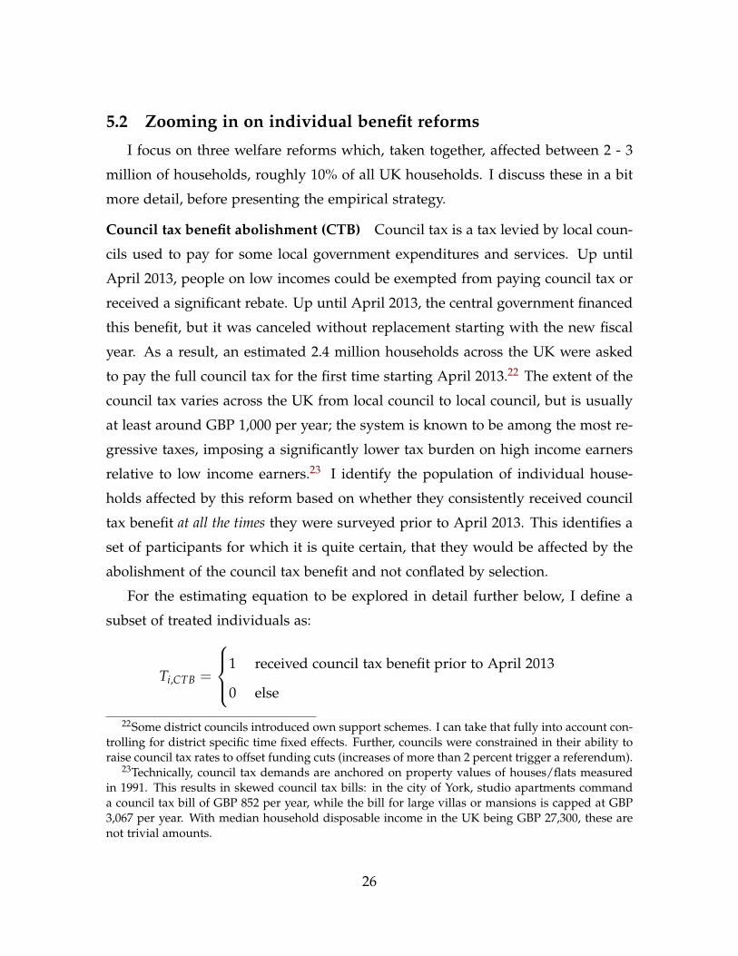
5.2 Zooming in on individual benefit reforms

I focus on three welfare reforms which, taken together, affected between 2 - 3

million of households, roughly 10% of all UK households. I discuss these in a bit

more detail, before presenting the empirical strategy.

Council tax benefit abolishment (CTB) Council tax is a tax levied by local coun-

cils used to pay for some local government expenditures and services. Up until

April 2013, people on low incomes could be exempted from paying council tax or

received a significant rebate. Up until April 2013, the central government financed

this benefit, but it was canceled without replacement starting with the new fiscal

year. As a result, an estimated 2.4 million households across the UK were asked

to pay the full council tax for the first time starting April 2013.22 The extent of the

council tax varies across the UK from local council to local council, but is usually

at least around GBP 1,000 per year; the system is known to be among the most re-

gressive taxes, imposing a significantly lower tax burden on high income earners

relative to low income earners.23 I identify the population of individual house-

holds affected by this reform based on whether they consistently received council

tax benefit at all the times they were surveyed prior to April 2013. This identifies a

set of participants for which it is quite certain, that they would be affected by the

abolishment of the council tax benefit and not conflated by selection.

For the estimating equation to be explored in detail further below, I define a

subset of treated individuals as:

Ti,CTB =

1 received council tax benefit prior to April 2013

0 else

22Some district councils introduced own support schemes. I can take that fully into account con-trolling for district specific time fixed effects. Further, councils were constrained in their ability toraise council tax rates to offset funding cuts (increases of more than 2 percent trigger a referendum).

23Technically, council tax demands are anchored on property values of houses/flats measuredin 1991. This results in skewed council tax bills: in the city of York, studio apartments commanda council tax bill of GBP 852 per year, while the bill for large villas or mansions is capped at GBP3,067 per year. With median household disposable income in the UK being GBP 27,300, these arenot trivial amounts.

26

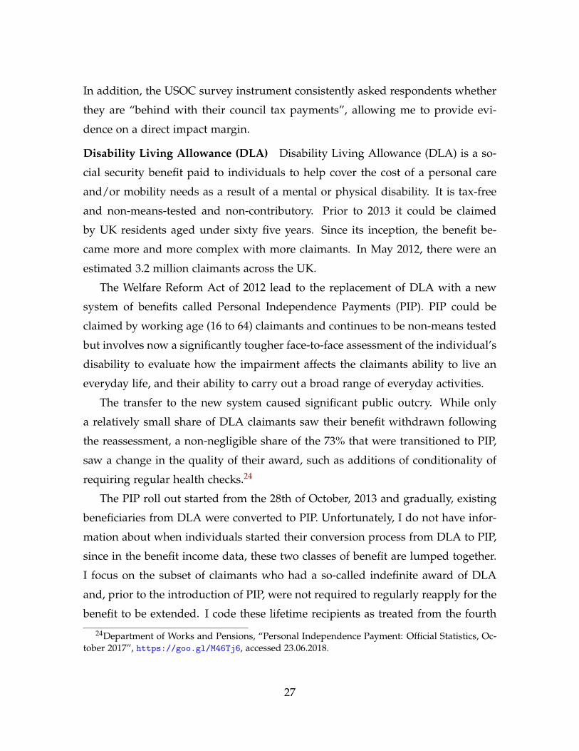
In addition, the USOC survey instrument consistently asked respondents whether

they are “behind with their council tax payments”, allowing me to provide evi-

dence on a direct impact margin.

Disability Living Allowance (DLA) Disability Living Allowance (DLA) is a so-

cial security benefit paid to individuals to help cover the cost of a personal care

and/or mobility needs as a result of a mental or physical disability. It is tax-free

and non-means-tested and non-contributory. Prior to 2013 it could be claimed

by UK residents aged under sixty five years. Since its inception, the benefit be-

came more and more complex with more claimants. In May 2012, there were an

estimated 3.2 million claimants across the UK.

The Welfare Reform Act of 2012 lead to the replacement of DLA with a new

system of benefits called Personal Independence Payments (PIP). PIP could be

claimed by working age (16 to 64) claimants and continues to be non-means tested

but involves now a significantly tougher face-to-face assessment of the individual’s

disability to evaluate how the impairment affects the claimants ability to live an

everyday life, and their ability to carry out a broad range of everyday activities.

The transfer to the new system caused significant public outcry. While only

a relatively small share of DLA claimants saw their benefit withdrawn following

the reassessment, a non-negligible share of the 73% that were transitioned to PIP,

saw a change in the quality of their award, such as additions of conditionality of

requiring regular health checks.24

The PIP roll out started from the 28th of October, 2013 and gradually, existing

beneficiaries from DLA were converted to PIP. Unfortunately, I do not have infor-

mation about when individuals started their conversion process from DLA to PIP,

since in the benefit income data, these two classes of benefit are lumped together.

I focus on the subset of claimants who had a so-called indefinite award of DLA

and, prior to the introduction of PIP, were not required to regularly reapply for the

benefit to be extended. I code these lifetime recipients as treated from the fourth

24Department of Works and Pensions, “Personal Independence Payment: Official Statistics, Oc-tober 2017”, https://goo.gl/M46Tj6, accessed 23.06.2018.

27

quarter 2013, when the roll out of PIP started. For the empirical design, this set of

affected individuals is identified as follows:

Ti,DLA =

1 always received either DLA or PIP

0 else

Technically, all DLA recipients with a lifetime award should receive a similar mon-

etary award through PIP, yet, the process and the requirement for regular assess-

ment is said to have caused significant grievances.25

Bedroom tax (BTX) Housing benefit is a benefit paid to individuals on low in-

come living in social rented housing. From April 2013 all current and future work-

ing age tenants renting from a local authority, housing association or other regis-

tered social landlord no longer receive help towards the costs of a spare room. This

provision was also dubbed the “bedroom tax” in the popular press as it implied

that a lot of working age parents, whose children had moved out, found them-

selves living in accommodation with an extra spare bedroom. The benefit allows

for one bedroom for each adult couple, for each single person over 16, for each 2

children of the same sex under 16 and for each 2 children of either sex under 10.

Individuals on low incomes claiming housing benefit who were found to have a

spare room as per these definitions saw a significant cut in the financial support to

pay rent by 14% when found to have one spare bedroom and 25% for those with

two or more spare bedrooms.

I identify individuals who were most likely affected by the “bedroom tax” as

follows. They must continuously live in social rented housing (roughly 16.4% of the

sample) and, they must have a spare bedroom as per the governments definition

the most recent time they were surveyed before April 2013.26 This defines a simple

25There were also significant concerns about the qualification of the staff tasked with the re-assessments, which were outsourced to two private firms. Anecdotes in media are rife withe.g. wheelchair-bound claimants being asked to attend a reassessment appointment in a non-accessible facilities, or claimants with down syndrome being asked when they “caught it”, seeThe Independent, “Disability benefit assessors failing to meet Government’s quality standards”,https://goo.gl/uX4yD5, accessed 23.06.2018.

26The requirement of living continuously in social rented housing is a conservative sample cut

28

treatment indicator used in the various difference-in-difference estimations.

Ti,BTX =

1 lives in social housing with excess bedroom(s) prior April 2013

0 else

The bedroom tax was widely debated in the popular press as it affected more than

660,000 households across the country. The Department of Works and Pensions

encouraged households to take in lodgers or to “move to accommodation which

better reflects the size and composition of their household.”27 I can directly mea-

sure two impact margins relevant to this benefit cut: the number of bedrooms in

the respondent’s accommodation after April 2013, and further, whether individ-

ual’s are reporting to be “behind with their rent”.

Combined treatment In addition to these three groups defining exposure to

treatment Ti,j with j ∈ {CTB,DLA,BTX} I also construct a combined dummy

Ti,ANY that takes on a value of 1, if a respondent household belongs to either

of these groups. In total, 10% of my USOC sample are affected by either of these

three treatments, which is similar when comparing to the aggregate estimate from

Beatty and Fothergill (2013), suggesting that between 2 - 3 million households

(around 10% of UK households) were affected by these three measures. I next

discuss the empirical strategy used.

5.3 Empirical strategy

As before, I will present results from pooled difference-in-difference designs as

well as event studies.

Pooled difference-in-difference I begin by estimating simple pooled difference-

in-differences, across a range of specifications that include more demanding sets

as some households attempting to avoid the bedroom tax may have moved to the private rentedsector due to limited availability of social housing. The spare bedroom indicator is constructedusing the information on the household composition and the age distribution of children allowinga near replication of the governments eligibility criteria.

27DWP Impact Assessment Housing Benefit: under-occupation of social housing, June 2012,https://goo.gl/xFWDqW.

29

of fixed-effects. The least demanding specification will be the equivalent to the

empirical specifications estimated in the previous sections, controlling for district-

and region specific non-linear time effects, but exploiting the individual level data.

The most demanding specification takes the following form:

yi,d,w,t = αi + βd,w,t + γ× Posti,j,t × Ti,j + εi,d,w,t (3)

In the above specification i indexes an individual respondent, so the inclu-

sion of individual level fixed effects αi imply that I exploit only within individual

variation. The time fixed effects, αd,w,t are specific to each of the 378 districts d,

survey wave w and time t measured in quarters. The specification fully absorbs

time varying district specific shocks affecting outcomes of respondents living in

the same district d commonly at time t, thus absorbing any changes in district

level policies that affect all individuals living in the same district.28 Importantly,

these district specific time effects also quite richly control for the indirect exposure

to austerity due to general equilibrium effects that the analysis of the local mul-

tipliers suggested. Making the time effects specific to the survey wave w further

controls for any survey wave specific idiosyncratic differences.

The main coefficient of interest is γ, which captures changes in the outcome

variables yi,d,w,t after a benefit cut j became effective on the subpopulation indi-

cated by Ti,j. The main outcome variable studied yi,d,w,t is a dummy variable indi-

cating whether respondents reveal a preference towards UKIP. In addition, I study

a range of reform specific auxiliary outcome measures that are either immediately

relevant to the welfare cuts, or capture political perceptions more broadly.

Event studies I also estimate a range of event studies for the specific benefit cuts,

using less demanding specifications, but exploiting fully frequency of the survey

data that arises due to the staggered data collection for the USOC waves.

The estimation specification is as follows:

28Such broader changes, e.g. closures of libraries or parks may also be a direct result of austerity.

30

yi,d,r,w,t = αd + βr,w,t +2015q4

∑t=2010q1

γt × Timet × Ti,j + εi,r,w,t (4)

This specification is almost identical to the specification studied when using

aggregate data with two differences. The time fixed effects βr,w,t are resolved at

the quarterly level specific to the survey wave w. I estimate a full set of quarter

time-effects γt, allowing me to draw event studies plots showing how the outcome

variables yi,d,r,w,t evolved over time relative to the timing specific to a reform j.

5.4 Results

I first discuss the results from the pooled difference-in-difference exercise, be-

fore turning to the event studies.

Pooled difference-in-difference The pooled difference-in-difference results are

presented in Table 3. The dependent variable in this table is a dummy indicating

whether an individual expressed support for UKIP. Columns 2-4 provide estimates

for the three different welfare reforms affecting different subpopulations, while

column 1 combines these into a single treatment indicator that gets switched on

after April 2013. The different Panels A - C employ different sets of fixed effects

for the estimation. Panel A employs simply district- and region by survey wave by

time fixed effects. This is the empirical design that comes closest to what was esti-

mated in the previous sections, exploiting district level variation. Throughout the

different welfare reforms, the population likely exposed to specific welfare reforms

is significantly more likely to express support for UKIP after these reforms became

effective. The point estimates are economically sizable, indicating that the treated

population sees an increase in the propensity to support UKIP by between 2.5 -

4.7 percentage points. In relative terms, the increase in the propensity to support

UKIP by between 53 - 100% (relative to the mean of the dependent variable which

stands at 4.7%). While the mean of the dependent variable appears low, suggesting

that the effects are driven by a small subpopulation, they should be seen relative

to other political parties. The Liberal Democrats, the UK’s third biggest party, sees

expressed support in the USOC population averaging at just 8.2%; hence, the UKIP

31

figures are not dramatically lower. Nevertheless, in the next section, I will explore

a set of broader outcome measures to allay some concerns about the validity of the

outcome measure.

Panel B only exploits within district variation, controlling for district by survey

wave by time fixed effects. This effectively controls for any idiosyncratic and time

varying shocks affecting all residents in a specific area. Such common shocks

could, e.g. be capturing the indirect economic effects of austerity affecting the

wider local economy or other local shocks. Throughout, the results remain very

similar across the different measures.

In Panel C finally, I only exploit within individual variation within districts,

controlling, in addition to the district by survey wave by time fixed effects, also

for individual level fixed effects. This comes at the cost of losing some statistical

power, yet, the results remain precisely estimated throughout.

Event studies I next turn to the event studies for the three different welfare re-

forms. I will use this also to provide some auxiliary evidence capturing effects

along margins immediately relevant to the individual welfare reforms.

I begin by studying the abolishment of council tax benefit. The results are pre-

sented visually in Figure 7. The left panel presents the average support for UKIP

among those individuals who have consistently received council tax benefit at all

times prior to its abolishment. The vertical line marks the date from which the

council tax benefit was abolished. The propensity of support for UKIP is consis-

tently higher, on average, after the benefit was abolished in this subpopulation.

Panel B presents evidence suggesting that the abolishment of council tax benefit

lead to increased economic pressures among those who received the benefit in the

past. The share of individuals in this group that states that they are in arrears with

their council tax payments rises sharply and in a very timely fashion.

Next, I turn to study the conversion of lifetime DLA claimants to PIP. This

result is presented in Figure 8. Again, with the reform becoming effective, the set

of likely lifetime claimants of disability living allowance see a marked increase in

their likelihood to support UKIP. There is no evidence that this particular benefit

32

increased direct economic grievances, but, this set of respondents is particularly

likely to state that they perceive that “government officials do not care”, suggesting

that the grievances were not direct economic but relate to the perceived treatment

by the welfare system.

Lastly, I turn to study the effects of the bedroom tax, which affected households

on low incomes living in social rented housing. The results are presented in Figure

9. The left panel presents the effects on support for UKIP among the group of

individuals affected by the bedroom tax. While the pattern is a bit more noisy,

there is a consistent increase in support for UKIP among this subpopulation. The

central panel explores an economic margin directly relevant to those individuals

who, likely, saw a cut to the housing benefit payment: they are significantly more

likely to be in arrears with their rent, suggesting that the cut to housing benefit

due to the spare bedroom increased rent arrears. Lastly, the right panel studies the

number of bedrooms as a response variable. This is immediately relevant as the

“bedroom tax” could be avoided if households moved to smaller accommodation.

The pattern is quite consistent, suggesting that households did indeed move to

smaller accommodation, thus avoiding some of the direct economic grievances.

Together, these results provide compelling evidence in support of the underly-

ing common trends assumption inherent to the previously presented difference-in-

difference estimates. Furthermore, for a few of the benefit cuts, I am able to show

adjustment margins immediately relevant to specific welfare reforms, highlight-

ing that the exposure to these reforms is likely to have created some grievances

relevant to inform political preferences. I next turn to study broader outcomes.

5.5 Broader outcome measures

Expressing political support for UKIP may only be one specific outcome mea-

sure, but the political responses to austerity could be much broader, such as sup-

port for the other political parties, general likes- or dislikes, or broader perceptions

of disenfranchisement or feeling treated badly and without political voice (which

in turn, are strong correlates of support for Leave as I will show).

I turn to two sets of other outcome measures.

33

Support and like or dislike for other parties I first present results capturing

shifts in expressions of support for other political parties. These are presented

in Table 4. Panel A suggests that there is a statistically significant and sizable

reduction in the support for the Conservative party. The underlying effect size

is similar in magnitude to the increase in support for UKIP that was observed.

There is more mixed evidence for the other political parties when studying specific

welfare reform measures in column (2) - (4). The results in the combined treatment

group in column (1) suggests that support for the left-leaning political parties

Labour and the Liberal Democrats increase among those affected by either of the

three welfare reforms. On the other hand, there is a reduction in those reporting

that they would not vote for any party if there was an election tomorrow (and are

neither a supporter, nor feel closer to any specific party) in Panel D. The latter

could suggest that some of the increase in support for UKIP may be drawn out

of this pool of potential voters, yet, in the Appendix I show this is not the case

(rather, Labour wins from this pool).29

In Appendix Table A3, I present results drawing on measures of the intensity of

like or dislikes of the three established political parties (the Conservatives, Labour

and the Liberal Democrats) on a 10 point Likert scale. The results suggest that,

respondents affected by the combined any welfare reform measure are much more

likely to express a scores indicating a strong dislikes for the Conservative party.

Perception of politics more broadly In Table 5, I present evidence for three addi-

tional survey questions, asking whether individuals perceive that “Public officials

do not care”, that they “Don’t have a say in what government does” and that “your

vote is unlikely to make a difference” when asked about the perceptions of the

relevance of the respondents vote in affecting general election outcomes in their

29This analysis is presented in Appendix Table A2. I construct a measure of the initial politicalparty preference the first instance respondents appear in the USOC data and estimate a heteroge-nous effect version, capturing how exposure to the combined any welfare reform treatment affects anindividual’s stated support for any political party as a function of the baseline political preferences.The results suggest that those who become UKIP supporters, are mostly original supporters of theConservatives, the Liberal Democrats and a few other parties and not drawn from individuals who,the first time they were surveyed, reported that they support no political party.

34

constituency. The perception of having no political voice is something that was

prominently leveraged in the EU referendum campaign, with voters being sug-

gested that voting against EU membership is a vote against the status quo (Ford

and Goodwin, 2017). Throughout each of these measures that governs the per-

ception of individuals of the public sector, the institution of voting or the feeling

of having no voice strongly and significantly increases in the population (likely)

affected by either of these three welfare reforms studies. This is consistent with

the idea that austerity contributed to a feeling of disenfranchisement or disconnect

from the established political parties and institutions, and encouraging voters to

support more extreme policy positions or engage in protest voting (Myatt, 2017).

I next show that exposure to welfare reforms – as per our above definitions –

not only increased propensity to support UKIP and increased perceived marginal-

ization – but is further, strongly linked to supporting Leave in the EU referendum.

5.6 Welfare reform exposure and support for Leave

The most recent wave of the USOC survey asks the EU referendum question. In

that data, Remain has a clear majority with only 43% of the respondents expressing

support for Leave. While the data for the this survey wave is still being collected

and not publicly released, a pre-release version has been made available to a se-

lected set of researchers working on Brexit topics.30 Appendix Figure A4 suggests

that, among the USOC respondents that express support for UKIP the most recent

time they were surveyed, 87% would support Leave, which non-surprisingly sug-

gests that the revealed expressions of support for UKIP are a good (time-varying)

proxy variable that picks up pro-Leave political preferences.

I estimate how the individual propensity to support Leave differs among in-

dividuals (likely) exposed to the specific welfare reforms, contrasting with other

individuals living in the same local authority districts, yet (likely) not exposed

30The data is expected to be released towards the end of 2018. I would like to thank NicoleMartin for her support and sharing details of the data. Alabrese et al. (2018) use the data toperform a horse race to assess the predictive power of individual versus aggregate level socio-economic variables in explaining leave voting tendencies.

35

to the austerity induced welfare-reforms.31 I estimate versions of the following

cross-sectional regression:

yi,d = β′Xi,d + γ× Ti,j + εi,d (5)

The above specification exploits variation in Leave-preferences between individu-

als i within a district d. I add iteratively richer sets of controls Xi,d and present the

estimated differential in leave support between individuals (likely) exposed to the

welfare reforms and those not.

The results are presented in Table 6. Moving across different columns, I itera-

tively add more demanding sets of control variables. In column (1), only include

district fixed effects are included. In column (2), I add the qualification group fixed

effects, column (3) adds age fixed effects allowing a different level of support for

Leave for respondents at each different age, column (4) adds employment status

fixed effects (in total ten different categories such as employed, unemployed, stu-

dent,..), column (5) adds gross household income decile fixed effects, column (6)

includes the industry of employment fixed effect across 19 different sectors (this

subsets the sample including only respondents in employment), column (7) con-

trols for socio-economic status group of the occupation (across eight categories),

while column (8) controls a set of dummy variables capturing whether individuals,

in the most recent survey, reported any of 17 different health conditions.32

The remarkable observation throughout is that the differential degree of sup-

port for Leave among individuals (likely) exposed to any of the three welfare

reforms studied in the previous sections is sizably and robustly larger. The set of

control variables that I add successively are particularly important, as they further

speak to the robustness of the results. In the motivating evidence presented in sec-

tion 3, I show that areas with significant shares of the local population having low

31The actual EU referendum results were not collected at a level finer than the district, whichserved as official counting areas. Hence, the USOC data is the only way to capture cross-sectionalmeasures of support for Leave, while controlling for district fixed effects.

32These health conditions include, among others, Asthma, Arthritis, Cancer or Malignant tu-mors, Diabetes, Depression, High Blood Pressure.

36

qualifications, being employed in retail- or manufacturing sector jobs or working

in routine jobs saw a significant uptick in electoral support for UKIP. In the results

in Table 6, I control for these characteristics measured at the individual level, and

observe that individuals likely exposed to any of the three welfare reforms see, on

average, about a 7 percentage points higher level of support for Leave.

Appendix Table A4 further shows that the additional outcome margins ex-

plored in the previous sections are also strong correlates of support for Leave over

and above what is captured by whether individuals report supporting UKIP, sug-

gesting that support for UKIP is a proxy that quite likely understates the extent

to which exposure to the welfare reforms may have contributed to the built up of

anti-EU political preferences culminating in the Leave vote.

In the last section, I shed some more light on longer running economic trends

and how the austerity-induced welfare reforms feature in that context, linking back

the findings to the existing literature.

6 Welfare cuts in context of longer running trendsThe extent to which the welfare state is functioning, cushioning out economic

shocks, is an important ingredient to maintain political support for globalization

or immigration. In this section, I link back to provide an understanding of the

broader economic context into which austerity, and the subsequent vote to leave

the EU falls. In order to be able to say something substantive about longer running

economic trends, I combine data from the earlier British Household Panel Study

(BHPS) and the later, Understanding Society survey data that I used in the pre-

vious sections. The BHPS is a much smaller study and was first launched in the

early 1990s. From 2001, it became a UK wide study.

Some of the roughly 8,000 BHPS participants continue to contribute to the

USOC panel study, since the BHPS was discontinued in 2008/2009. The USOC

and the BHPS data can be harmonized and combined on some central questions,

such as benefit-, labor- and gross income as well as basic measures of human cap-

ital, employment status and sector of employment. This allows a further view of

37

the data, in particular, to shed light on the relative evolution of different types of

incomes, particularly, along the human capital divide. The consistent and recur-

ring feature of cross-sectional analysis of populist voting suggest that support is

significantly concentrated in population strata with relatively low human capital.

These are also the areas, that typically also most reliant on the welfare state.

Estimating robust trends Combining the data from the BHPS survey rounds 11-

18 and the USOC data, I can exploit a representative panel over this 15 year period,

exploiting only within individual variation.

In particular, I estimate

yi,d,r,w,t = αi + βd,w,t +2015

∑t=2001

γt × Timet × Xi,t + εi,r,w,t (6)

The dependent variable yi,d,r,w,t measures either the individual level monthly

labor-, benefit- and gross incomes over time. This specification controls for indi-

vidual respondent fixed effects αi, exploiting the fact that both the USOC and the

BHPS are panels, where some of the BHPS respondents continue to contribute to

USOC. Further, I control flexibly for local authority district by survey wave and

year fixed effects, controlling in a very parsimonious fashion for district specific

economic development. The coefficients of interests are the point estimates on γt,

capturing the extent to which an individual i’s educational attainment correlates

with the evolution of individual income (by source) over time, exploiting only

individual level variation between residents living in the same district.33

Results The results are visually presented in Figure 10. Panel A presents the

trends pertaining to respondents with low human capital, that is, no formal qual-

ifications and no secondary school leaving certificate. The results suggest that

throughout the last 15 years, monthly labor incomes for those with low human

capital has, in relative terms, evolved negatively. Relative to the rest of the pop-

ulation, low human capital individuals had a slight labor income premium at the

onset, but this has been gradually eroded over time, turning negative, indicat-

33Individual survey participants may move across the UK between different census rounds. Thepatterns presented here are robust to removing movers from the estimating sample.

38

ing that relative to the rest of the population, labor incomes have fallen short.

The central panel in Panel A presents the evolution of monthly benefit income.

While that stays flat for the early years in the 2000s, from around 2005 onwards,

there is a steady growth in benefit incomes to individuals with low human cap-

ital. This trend growth comes to an abrupt halt from 2011 onwards. The last

column presents gross income, that includes labor-, and benefit income. For most

of the earlier 2000’s gross income for individuals with low educational attainment

is trending downwards, this trend is flattened out for the period between 2008

to 2012, as benefit income is evening out the relative income losses. From 2014

onwards, there are marked drops in gross income.

Panel B studies the trends pertaining to respondents with high human capi-

tal, having completed at least an undergraduate university degree. Labor income

for this group of individuals has trended up significantly over time in an uninter-

rupted fashion. Benefit income, which for those groups of individuals are most

likely the non non-means tested child benefit, which only became means tested

from 2013 onwards, is trending down and flattens out as well post 2011. This

suggests that both, high income as well as low income earners were affected by

austerity. Yet, while gross incomes fell in relative terms for those with low human

capital, it continued to grow for individuals with a university degree.

This suggests three things: first, while labor income for individuals at the lower

end of the skill divide saw significant downward trends over time, it markedly in-

creased in relative terms for those at the top end of the human capital divide, sug-

gesting significant increase in the skill-divide (Card and DiNardo, 2002; Lemieux,

2006). Second, the welfare state was responsive, evening out these growing in-

equalities, yet this came to an abrupt halt as the Conservative-led coalition gov-

ernment’s austerity measures took effect. Third, gross income inequality is likely

to have increased since 2010, as the positive trend growth in labor and gross in-

come for those with university degrees continues.

Discussion Linking back to the existing literature, in particular, the seminal work

by Autor et al., 2013 which documents how trade integration with China lead to

39

job losses and economic grievances in the context of the US. The patterns presented

here suggest that the welfare state in the UK was quite responsive, and may have

helped cushioning the political cost of trade integration. Nevertheless, as shown

in Appendix Figure A5, the patterns presented here are robust to only includ-

ing individuals that have never reported to have worked in either manufacturing,

agriculture or mining. These sectors are the ones that are typically considered to

be directly affected by the economic pressures of trade integration in this litera-

ture. This evidence, in addition to the previous results suggests that the economic

grievances and the secular relative decline in labor incomes for those with low hu-

man capital, can not be explained studying trade integration alone. Other factors,

such as general structural transformation (Rogerson, 2008; Rodrik, 2016), the rise

of automation (Caprettini and Voth, 2015; Graetz and Michaels, 2015), skill-biased

technological change more broadly (Acemoglu, 1998; Autor et al., 1998, 2003), the

rise of the gig economy or possibly migration affecting wages at the lower end of

the wage distribution (Becker and Fetzer, 2018; Dustmann et al., 2013) are likely to

feature among additional important explanations behind these trends.

What combines these developments is that an active welfare state can help even

out the distributional effects caused by the underlying trends and may thus help

to maintain popular support e.g. for continued trade integration or migration.34

This paper suggests that, reforms to the welfare state, likely also creating losers,

may cause a significant political backlash.

7 ConclusionThe UK’s decision to leave the EU is a watershed moment in European history,

marking an end to a seventy year process of continued economic and political in-

tegration. Understanding the underlying causes for why the UK’s electorate voted

to Leave the EU is of utmost importance – not only for the UK as it disentangles it-

self from the European project – but for many other European countries, that see a

34Hassler et al. (2003) provide a formal argument suggesting that skill-biased technical changemay undermine the viability of the welfare state.

40

growth in support for political parties campaigning on anti-EU political platforms.

This paper presents novel and comprehensive evidence suggesting that austerity-

induced welfare reforms brought about by the Conservative-led coalition govern-

ment from late 2010 onwards are key to understanding Brexit. Austerity-induced

welfare reforms are a strong driving factor behind the growing support for the

populist UKIP party in the wake of the EU referendum, contributed to the devel-

opment of broader anti-establishment preferences and are strongly associated with

popular support for Leave. The results suggest that the EU referendum either may

not have taken place, or, as a back of the envelope calculations suggests, could have

resulted in a victory for Remain, had it not been for austerity. By combining evi-

dence from the population of all electoral contests in the UK since 2000, together

with a wealth of evidence stemming from individual level panel data, this paper

is among the more comprehensive studies of the UK’s political landscape around

the EU referendum thus far.

While exposure to austerity-induced welfare reforms is a key activating factor,

contributing to the build up of anti-EU preferences and support for populist par-

ties, the underlying economic causes that lie behind the growing reliance and expo-

sure of (especially low skilled) individuals on the welfare state is of key relevance

to the broader public and political debate. This paper provides some suggestive

auxiliary evidence indicating that factors contributing to the growing skill-divide

in labor markets are likely to go beyond trade-integration alone, which is a key

driver explored in an important growing literature.

Important future work is needed to systematically take stock to quantify the

relative contribution of the range of factors contributing to the development of

(relative) economic grievances along key socio-economic fault lines. This can help

inform political decision making and contribute to the design of welfare-systems

ready for the 21st century.

ReferencesAcemoglu, D. (1998). Why Do New Technologies Complement Skills? Directed

Technical Change and Wage Inequality. The Quarterly Journal of Economics 113(4),1055–1089.

41

Aksoy, C. G., S. Guriev, and D. Treisman (2018). Globalization, Government Popu-larity, and the Great Skill Divide.

Alabrese, E., S. O. Becker, T. Fetzer, and D. Novy (2018). Who Voted for Brexit ?Individual and Regional Data Combined. mimeo (March).

Alesina, A., R. Perotti, and J. Tavares (1998). The political economy of fiscal adjust-ments. Brooking Papers on Economic Activity 1(1), 197–266.

Alesina, A., E. Spolaore, and R. Wacziarg (2000). Economic Integration and Politi-cal Disintigration. American Economic Review 90(5), 1276–1296.

Alesina, A. F., D. Carloni, and G. Lecce (2011). The Electoral Consequences ofLarge Fiscal Adjustments. NBER Working Paper Series, 4–7.

Anderson, C. J. and M. S. Reichert (1995). Economic Benefits and Support forMemebership in the EU.: A Cross-National Analysis. Journal of Public Pol-icy 15(3), 231–249.

Antras, P., A. De Gortari, and O. Itskhoki (2016). Globalization, Inequality andWelfare. NBER Working Paper Series (22676).

Arias, E. and D. Stasavage (2016). How Large Are The Political Costs of FiscalAusterity?

Arzheimer, K. (2009). Contextual Factors and the Extreme Right Vote in WesternEurope , 1980 – 2002. American Journal of Political Science 53(2), 259–275.

Autor, D., D. Dorn, G. Hanson, and K. Majlesi (2016). Importing Political Polar-ization? The Electoral Consequences of Rising Trade Exposure. CEPR DiscussionPaper 11511.

Autor, D. H., D. Dorn, and G. H. Hanson (2013). The China Syndrome: Local labormarket impacts of import Competition in the United States. American EconomicReview 103(6), 2121–2168.

Autor, D. H., L. F. Katz, and A. B. Krueger (1998). Computing Inequality: HaveComputers Changed the Labor Market? The Quarterly Journal of Economics 113(4),1169–1213.

Autor, D. H., F. Levy, and R. J. Murnane (2003). The skill content of recent techno-logical change: An empirical exploration. Quarterly Journal of Economics 118(4),1279–1333.

Barone, G., A. D’Ignazio, G. de Blasio, and P. Naticchioni (2016). Mr. Rossi, Mr.Hu and politics. The role of immigration in shaping natives’ voting behavior.Journal of Public Economics 136(8228), 1–13.

Barsbai, T. and H. Rapoport (2017). From exodus to exitus: Selective emigrationafter Germany ’ s failed 1848 revolutions and the rise of the Nazi Party. mimeo.

42

Beatty, C. and S. Fothergill (2013). Hitting the poorest places hardest: The localand regional impact of welfare reform. Technical report.

Becker, S. O. and T. Fetzer (2018). Has Eastern European Migration ImpactedBritish Workers ? mimeo.

Becker, S. O., T. Fetzer, and D. Novy (2017). Who voted for Brexit? A comprehen-sive district-level analysis. Economic Policy 32(92), 601–650.

Blumenau, J., A. C. Eggers, D. Hangartner, and S. Hix (2017). Open/Closed Listand Party Choice: Experimental Evidence from the UK. British Journal of PoliticalScience 47(4), 809–827.

Borjas, G. J. (2003). The labor demand curve is downward sloping: Reexaminingthe impact of immigration on the labor market. The Quarterly Journal of Eco-nomics 118(4), 1335–1374.

Born, B., G. J. Muller, M. Schularick, and P. Sedlacek (2018). The Costs of EconomicNationalism: Evidence from the Brexit Experiment. CEPR Discussion Paper.

Breinlich, H., E. Leromain, D. Novy, and T. Sampson (2017). The Consequences ofthe Brexit Vote for UK Inflation and Living Standards: First Evidence. mimeo.

Bursztyn, L., D. Cantoni, P. Funk, and N. Yuchtman (2017). Polls, the Press, andPolitical Participation: The Effects of Anticipated Election Closeness on VoterTurnout. NBER Working Paper.

Caprettini, B. and H.-J. Voth (2015). Rage Against the Machines: Labor-SavingTechnology and Unrest in England, 1830-32. mimeo 29(33), 1–9.

Card, D. and J. DiNardo (2002). Skill Biased Technological Change and RisingWage Inequality: Some Problems and Puzzles. Journal of Labor Economics 20(4),733–783.

Che, Y., Y. Lu, J. R. Pierce, P. K. Schott, and Z. Tao (2017). Did Trade Liberalizationwith China Influence U.S. Elections? mimeo.

Colantone, I. and P. Stanig (2018). Global Competition and Brexit. American PoliticalScience Review 112(02), 201–218.

Colussi, T., I. E. Isphording, and N. Pestel (2017). Minority Salience and PoliticalExtremism. mimeo 49(0), 4–5.

Dehdari, S. (2017). Economic Distress and Support for Far-right Parties: Evidencefrom Sweden. Unpublished Manuscript, 2017.

Dhingra, S., H. Huang, G. Ottaviano, J. Paulo Pessoa, T. Samson, and J. Van Reenen(2017). The costs and benfits of leaving the EU: trade effects. Economic Pol-icy (February 2018), 651–705.

Dippel, C., R. Gold, and S. Heblich (2015). Globalization and Its (Dis-)Content:Trade Shocks and Voting Behavior. NBER Working Paper 21812.

43

Dustmann, C., T. Frattini, and I. P. Preston (2013). The effect of immigration alongthe distribution of wages. Review of Economic Studies 80(1), 145–173.

Dustmann, C., K. Vasiljeva, and A. Piil Damm (2018). Refugee Migration andElectoral Outcomes. forthcoming, Review of Economic Studies.

Ford, R. and M. Goodwin (2017). Britain After Brexit: A Nation Divided. Journalof Democracy 28(28), 17–30.

Ford, R., M. J. Goodwin, and D. Cutts (2012). Strategic Eurosceptics and politexenophobes: Support for the United Kingdom Independence Party (UKIP) in the2009 European Parliament elections. European Journal of Political Research 51(2),204–234.

Gabel, M. (1998). Public Support for European Integration: An Empirical Test ofFive Theories. The Journal of Politics 60(2), 333–354.

Galofre-Vila, G., C. M. Meissner, M. McKee, and D. Stuckler (2017). Austerity andthe rise of the Nazi party. NBER Working Paper No. 24106.

Goodwin, M. and O. Heath (2016). The 2016 Referendum, Brexit and the LeftBehind: An Aggregate-Level Analysis of the Result. The Political Quarterlly.

Goodwin, M., S. Hix, and M. Pickup (2018). For and Against Brexit: A SurveyExperiment of the Impact of Campaign Effects on Public Attitudes toward EUMembership. British Journal of Political Science, 1–15.

Gorodnichenko, Y., T. Pham, and O. Talavera (2016). Social network , sentimentand political outcomes : Evidence from # Brexit. mimeo.

Graetz, G. and G. Michaels (2015). Robots at work. forthcoming, Review of Economicsand Statistics.

Grossman, G. M. and E. Rossi-Hansberg (2008). Trading Tasks: A Simple Theoryof Offshoring. American Economic Review 98(5), 1978–1997.

Guiso, L., H. Herrera, M. Morelli, and T. Sonno (2018). Populism: Demand andSupply. Mimeo, 1–63.

Hainmueller, J. and D. J. Hopkins (2014). Public Attitudes Toward Immigration.Annual Review of Political Science 17(1), 225–249.

Halla, M., A. Wagner, and J. Zweimuller (2017). Immigration and Voting for theExtreme Right. Journal of the European Economic Association.

Hassler, J., J. V. Rodrıguez Mora, K. Storesletten, and F. Zilibotti (2003). The Sur-vival of the Welfare State. American Economic Review 93(1), 87–112.

Hobolt, S. B. (2016). The Brexit vote: a divided nation, a divided continent. Journalof European Public Policy 23(9), 1259–1277.

44

Hobolt, S. B. and C. E. de Vries (2016). Public Support for European Integration.Annual Review of Political Science 19(1), 413–432.

Ilzetzki, E., E. G. Mendoza, and C. A. Vegh (2013). How big (small?) are fiscalmultipliers? Journal of Monetary Economics 60(2), 239–254.

Inglehart, R. and P. Norris (2016). Trump, Brexit, and the Rise of Populism: Eco-nomic Have-Nots and Cultural Backlash. SSRN Electronic Journal.

Innes, D. and G. Tetlow (2015). Delivering Fiscal Squeeze by Cutting Local Gov-ernment Spending. Fiscal Studies 36(3), 303–325.

Krugman, P. and A. Venables (1995). Globalization and the Inequality of Nations.Quarterly Journal of Economics 110(4), 2–4.

Lemieux, T. (2006). Increasing Residual Wage Inequality: Composition Effects,Noisy Data, or Rising Demand for Skill? American Economic Review 96(3), 461–498.

Lynch, P. and R. Whitaker (2013). Rivalry on the right: The Conservatives, the UKIndependence Party (UKIP) and the EU issue. British Politics 8(3), 285–312.

Mayda, A. M., G. Peri, and W. Steingress (2016). Immigration To the U.S.: aProblem for the Republicans or the Democrats? NBER Working Paper Se-ries 21941(9543).

Moretti, E. (2010). Local Multipliers. American Economic Review 100(2), 373–377.

Myatt, D. P. (2017). A Theory of Protest Voting. Economic Journal 127(603), 1527–1567.

Ottaviano, G. I. P. and G. Peri (2012). Rethinking the Effects of Immigration onWages. Journal of the European Economic Association 10(1), 152–197.

Piketty, T. (2018). Brahmin Left vs Merchant Right: Rising Inequality and theChanging Structure of Political Conflict, Evidence from France & the US, 1948-2017. (March), 1948–2017.

Ponticelli, J. and H.-J. Voth (2017). Austerity and Anarchy: Budget Cuts and SocialUnrest in Europe, 1919-2008. mimeo.

Revenga, A. A. L. (1992). Exporting Jobs ?: The Impact of Import Competitionon Employment and Wages in U . S . Manufacturing. The Quarterly Journal ofEconomics 107(1), 255–284.

Rodrik, D. (2000). How far will Economic Integration Go? Journal of EconomicPerspectives 14(1), 177–186.

Rodrik, D. (2016). Premature deindustrialization. Journal of Economic Growth 21(1),1–33.

45

Rogerson, R. (2008). Structural Transformation and the Deterioration of EuropeanLabor Market Outcomes. Journal of Political Economy 116(2), 235–259.

Scheve, K. and M. J. Slaughter (2004). Economic Insecurity and the Globalizationof Production. American Journal of Political Science 48(4), 662–674.

Scheve, K. F. and M. J. Slaughter (2001a). Labor Market Competition and Individ-ual Preferences Over Immigration Policy. Review of Economics and Statistics 83(1),133–145.

Scheve, K. F. and M. J. Slaughter (2001b). What determines individual trade-policypreferences? Journal of International Economics 54(2), 267–292.

Spolaore, E. (2013). What Is European Integration Really About? A Political Guidefor Economists. Journal of Economic Perspectives 27(3), 125–144.

Steinmayr, A. (2016). Contact Matters: Exposure to Refugees and Voting for theFar-Right. mimeo (April).

Stiglitz, J. (2002). Globalization and its Discontents. Penguin.

Stolper, W. F. and P. A. Samuelson (1941). Protection and Real Wages. The Reviewof Economic Studies 9(1), 58–73.

Voigtlander, N. and H. Voth (2017). Highway to Hitler. NBER Working Paper.

Webb, P. and T. Bale (2014). Why do tories defect to ukip? Conservative partymembers and the temptations of the populist radical right. Political Studies 62(4),961–970.

46

Figure 1: UKIP Election Result in 2014 EP elections and EU referendum vote leave.

Notes: The R-squared of a univariate cross-sectional regression of support for Leave and UKIP vote share in the 2014elections is 75%, and the point estimate is a near straight line with an intercept of 15 percentage points, suggesting thatUKIP EP vote share plus 15% does a reasonably good job predicting the EU referendum vote share for Leave.

47

Figure 2: UKIP vote share in the EP elections in 2004, 2014 and the Leave share in the 2016 EU referendum

Panel A: UKIP vote in 2004 Panel B: UKIP Vote in 2014 Panel C: Leave share

Notes: This map displays the UKIP vote share in the European Parliamentary elections in 2004 and 2014 in Panel A and B, and the share of the electorate that voted leave inthe 2016 EU referendum across local authority districts in Panel C.

48

Figure 3: Non-parametric effect of educational qualification, socio-economic status,and sectoral employment of the resident population as of 2001 on support for UKIPover time

Panel A: No qualifications Panel B: Routine jobs

Panel C: Retail Panel D: Manufacturing

Notes: The dependent variable is the percentage of votes for UKIP in local council elections. Panel A uses the share of theresident population with no formal qualifications as of 2001. Panel B uses the share of the resident population in Routinejobs as per the National Socio-Economic Classification of Occupations as of 2001. Panel C uses the share of the residentworking age population employed in the Retail sector, while panel D uses the share of the resident working age populationemployed in Manufacturing. The graph plots point estimates of the interaction between these cross sectional measures anda set of year fixed effects. All regression include local authority district fixed effects and NUTS1 region by year fixed effects.Standard errors are clustered at the district level with 90% confidence bands indicated.

49

Figure 4: Aggregate real government spending per capita over time across threebroad spending categories across the different tiers of government

Notes: Figure plots real aggregate spending per capita using data from HMRC for the years between 2000-2015. Aggregatetotals are divided by total population from the National Office of Statistics and the annual CPI with 2015 being the baseyear. The four series account for – on average – account for 68% of government spending over the sample period.

50

Figure 5: Distribution of austerity shock across local authority districts across theUK

Notes: This map displays the spatial distribution of the Austerity shock across local authority areas in the UK. The sizeof the shock is measured as the anticipated losses in benefit income per working age individual and year from Beatty andFothergill (2013)..

51

Figure 6: Non-parametric effect of austerity on support for UKIP overall and byindividual measures.

Panel A: Overall austerity shock Panel B: Council Tax Benefit

Panel C: Disability Living Allowance Panel D: Bedroom Tax

Notes: The dependent variable is the percentage of votes for UKIP in English and Welsh local council elections from 2000-2015. The graph plots point estimates of the interaction between these simulated incidence of the austerity measures and aset of year fixed effects. All regression include local authority district fixed effects and NUTS1 region by year fixed effects.Standard errors are clustered at the district level with 90% confidence bands indicated.

52

Figure 7: Impact of abolishment of national council tax benefit system effective April 2013 on support for UKIP andbeing behind on council tax payments

Effect of “council tax benefit” abolishment on...

support for UKIP being in arrears with council tax payments

Notes: Figure plots event studies studying the impact of the abolishment of council tax benefit on previous recipients. The dependent variable in the left panel is a dummyvariable indicating whether the respondent revealed a political preference in support of UKIP. The dependent panel in the right hand side is an indicator variable indicatingwhether the respondent is behind with his or her council tax payments. The regressions control for counil by survey wave by time fixed effects. The graph plots point estimatesof the interaction between an indicator variable indicating whether the individual respondents received council tax benefit at each point in time in the three years prior to thereform in which they were observed in the sample interacted with an indicator for the survey quarter. Standard errors are clustered at the district level with 95% confidencebands indicated.

53

Figure 8: Impact of “disability living allowance” conversion starting October 282013 on support for UKIP

Notes: Figure plots event studies studying the impact of the abolishment of council tax benefit on previous recipients. Thedependent variable in the left panel is a dummy variable indicating whether the respondent revealed a political preferencein support of UKIP. The dependent panel in the right hand side is an indicator variable indicating whether the respondentis behind with his or her council tax payments. The regressions control for counil by survey wave by time fixed effects. Thegraph plots point estimates of the interaction between an indicator variable indicating whether the individual respondentsreceived council tax benefit at each point in time in the three years prior to the reform in which they were observed inthe sample interacted with an indicator for the survey quarter. Standard errors are clustered at the district level with 95%confidence bands indicated.

54

Figure 9: Impact of “bedroom tax” effective April 2013

Effect of “bedroom tax” penalizing social housing tenants on low incomes with spare bedrooms on...

support for UKIP being in arrears with rent number of bedrooms in domicile

Notes: Figure plots event studies studying the impact of the bedroom tax penalizing households receiving housing benefit living in social housing and are judged to havea spare bedroom. The dependent variable in the left panel is a dummy variable indicating whether the respondent revealed a political preference in support of UKIP. Thedependent panel in the center column is an indicator whether respondents state that they are in arrears with their rent, while the outcome variable in the right panel is thenumber of bedrooms in the dwelling that a respondent lives in. The regressions control for council by survey wave by time fixed effects. The graph plots point estimates ofthe interaction between an indicator variable indicating whether the individual respondents are living in social rented housing at each point in time observed in the data andare judged to have an extra bedroom at the most recent time they were surveyed relative to the reform becoming effective in April 2013. Standard errors are clustered at thedistrict level with 95% confidence bands indicated.

55

Figure 10: Non-parametric estimates capturing the evolution of labor and benefit income within individuals over timefor respondents with low- and high levels of educational attainment

Panel A: Evolution of benefit and labor income for individuals with no qualifications

Labor income Benefit income Gross income

Panel B: Evolution of benefit and labor income for individuals with university degree

Labor income Benefit income Gross income

Notes: The dependent variable is the monthly gross labor income on the left, and the monthly benefit income on the right. The population is restricted to the sample of BHPSand USOC respondents that are not retired. The BHPS survey waves 11-18 start in 2001 and end in 2009, while the larger USOC survey starts in 2009 and includes some, butnot all of the former BHPS respondents. The graph plots point estimates of the interaction between the qualification status of respondents (having no qualifications in toprow, versus having a university degree in bottom row) on monthly labor or benefit income. All regression include individual respondent fixed effects and local authority bysurvey wave by time fixed effects. Standard errors are clustered at the district level with 90% confidence bands indicated.

56

Table 1: The Impact of different austerity measures on support for UKIP across Local, Euro-pean and Westminster elections

(1) (2) (3) (4) (5) (6)Overall TC CB CTB DLA BTX

Panel A: Local1(Year>2010) × Austerity 0.014*** 0.081*** 0.036 0.128*** 0.166*** 0.162*

(0.003) (0.013) (0.044) (0.036) (0.031) (0.086)Mean of DV 4.49 4.49 4.49 4.49 4.49 4.49Local authority districts 345 346 346 346 346 346Observations 3260 3263 3263 3263 3263 3263

Panel B: European1(Year>2010) × Austerity 0.008*** 0.049*** 0.054* 0.060** 0.128*** 0.001

(0.002) (0.009) (0.028) (0.028) (0.018) (0.047)Mean of DV 21.1 21.1 21.1 21.1 21.1 21.1Local authority districts 378 379 379 379 379 379Observations 1134 1137 1137 1137 1137 1137

Panel C: Westminster1(Year>2010) × Austerity 0.008*** 0.076*** -0.025 0.064 0.178*** 0.043

(0.002) (0.009) (0.025) (0.041) (0.021) (0.030)Mean of DV 6.03 6.03 6.03 6.03 6.03 6.03Harmonized Constituencies 566 566 566 566 566 566Observations 2047 2047 2047 2047 2047 2047

Avg Loss per working age adult 447.1 87.97 71.52 7.21 36.57 10.81Affected HH. in 1000s 4507 7601 2436 499 660Correlation with...

No qualification share .75 .17 .51 .77 .58Routine job share .6 .12 .27 .62 .43Retail sector share .35 .28 .02 .21 .08Manufacturing sector share .3 .11 -.03 .37 .24

Notes: Table reports results from a panel OLS regressions with the dependent variable being UKIP’s voteshare in English and Welsh Local Elections from 2000 to 2015 in Panel A, European Elections in Panel B andWestminster Elections in Panel C. The regressions control for local authority district fixed effects in Panels Aand B, and harmonized constituency level in panel C as well as NUTS1 region by year fixed effects throughout.Standard errors clustered at the Local Government Authority District Level in Panel A and B and at theHarmonized Constituency level in Panel C, with standard errors presented in parentheses, stars indicate ***p < 0.01, ** p < 0.05, * p < 0.1.

57

Table 2: The Impact of different austerity on local area gross value added by sector with spending multiplier estimates

(1) (2) (3) (4) (5) (6) (7)Sector Overall Retail & Distr. Public admin Manuf. Business Serv. Construction Financial Serv.

1(Year>2010) × Total Austerity Impact -0.008** -0.010** 0.004 -0.032*** -0.006 -0.010 -0.010(0.000) (0.000) (0.000) (0.000) (0.000) (0.000) (0.000)

Sector GVA 33440 6338 5936 4051 3692 2226 2031Implied multiplier effect -2.51 -.62 .23 -1.29 -.23 -.22 -.2UKIP vote share IV estimate -175.55** -137.82** 1862.58 -40.74*** -239.12 -177.51 -75.14

(73.65) (58.22) (9747.29) (13.42) (369.69) (169) (58.08)Local election districts 345 345 345 345 345 345 345Observations 5520 5520 5520 5520 5520 5520 5520

Notes: Table reports results from a panel OLS regressions with local authority area and region by year fixed effects. The dependent variable is the log value of the sectorspecific gross value added per working age adult in a local authority area between 2000 to 2015. The multiplier effect is the size of the contraction in gross value added dueto a one pound contraction in benefit payments due to austerity. The IV estimate presents the link between the contractions in gross value added due to austerity after 2010to the increasing support for UKIP. A negative coefficient suggests that areas with high incomes due to little austerity exposure see no growth in support for UKIP in localelections. Standard errors clustered at the Local Government Authority District Level are presented in parentheses, stars indicate *** p < 0.01, ** p < 0.05, * p < 0.1.

58

Table 3: The Impact of different austerity measures on support for UKIP: exploitingindividual level data

(1) (2) (3) (3)Any CTB DLA BTX

Panel A:Post × Benefit cut 0.026*** 0.026*** 0.047*** 0.024***

(0.005) (0.005) (0.012) (0.008)Mean of DV .0472 .0472 .0472 .0469Local election districts 379 379 379 379Observations 252642 252642 252642 245352District FE & Region x Wave x Time FE x x x x

Panel B:Post × Benefit cut 0.024*** 0.025*** 0.038*** 0.021**

(0.005) (0.005) (0.012) (0.009)Mean of DV .0472 .0472 .0472 .0469Local election districts 379 379 379 379Observations 252642 252642 252642 245352District x Wave x Time FE x x x x

Panel C:Post × Benefit cut 0.017*** 0.019*** 0.029** 0.011

(0.005) (0.006) (0.014) (0.008)Mean of DV .0472 .0472 .0472 .0469Local election districts 379 379 379 379Observations 252642 252642 252642 245352Individual FE & District x Wave x Time FE x x x x

Notes: Table reports results from a panel OLS. The dependent variable is a dummy variable taking thevalue 1 in case a respondent expresses support for UKIP. The columns indicate the different welfarereforms we study. Panel A controls for district by NUTS 1 Region x Wave x Time fixed effects, thusexploiting between district and between individual variation. Panel B controls for District x Wavex Time Fixed effects, thus only exploiting between individual variation within a district. Panel Ccontrols for Respondent fixed effects and District x Wave x Time Fixed Effects, exploiting only withinindividual- and within district variation. Standard errors clustered at the Local Government AuthorityDistrict Level are presented in parentheses, stars indicate *** p < 0.01, ** p < 0.05, * p < 0.1.

59

Table 4: The Impact of different austerity measures on support for other parties:Exploiting individual level data

(1) (2) (3) (4)Any CTB DLA BTX

Panel A: Support for ConservativesPost × Benefit cut -0.023*** -0.018*** -0.022** -0.030***

(0.005) (0.005) (0.011) (0.007)Mean of DV .259 .259 .259 .261Local election districts 379 379 379 379Observations 251310 251310 251310 244068

Panel B: Support for LabourPost × Benefit cut 0.016*** 0.017** 0.002 0.022*

(0.006) (0.007) (0.014) (0.011)Mean of DV .351 .351 .351 .348Local election districts 379 379 379 379Observations 251310 251310 251310 244068

Panel C: Support for Liberal DemocratsPost × Benefit cut 0.008** 0.003 -0.003 0.018***

(0.003) (0.004) (0.009) (0.005)Mean of DV .0815 .0815 .0815 .0828Local election districts 379 379 379 379Observations 251310 251310 251310 244068

Panel D: Support for No partyPost × Benefit cut -0.013** -0.015** 0.005 -0.017

(0.006) (0.007) (0.013) (0.012)Mean of DV .193 .193 .193 .193Local election districts 379 379 379 379Observations 251310 251310 251310 244068

Individual FE x x x xDistrict x Wave x Time FE x x x x

Notes: Table reports results from a panel OLS regressions. The dependent variable is a dummyindicating individual USOC respondent’s support for the Conservatives (panel A), the Labour party(panel B) and the Liberal Democratic party (panel C). The regressions include various differentlevels of fixed effects indicated at the bottom of the table. Standard errors clustered at the LocalGovernment Authority District Level are presented in parentheses, stars indicate *** p < 0.01, **p < 0.05, * p < 0.1.

60

Table 5: Wider measures of perceptions of disenfranchisement: included only inWave 2,3 and 6 of USOC study

(1) (2) (3)

Panel A: Public officials dont carePost × Benefit cut 0.068*** 0.062*** 0.053

(0.021) (0.023) (0.041)Mean of DV 3.37 3.37 3.37Local election districts 378 378 378Observations 75547 75547 75547

Panel B: Don’t have say in what govt doesPost × Benefit cut 0.088*** 0.078*** 0.071*

(0.020) (0.022) (0.042)Mean of DV 3.34 3.34 3.34Local election districts 378 378 378Observations 75897 75897 75897

Panel C: Your vote is unlikely to make a differencePost × Benefit cut 0.035*** 0.038*** 0.043**

(0.011) (0.012) (0.021)Mean of DV .563 .563 .563Local election districts 378 378 378Observations 74947 74947 74947

District FE xRegion x Wave x Time FE xDistrict x Wave x Time FE x xIndividual FE x

Notes: Table reports results from a panel OLS regressions. The dependent variable in Panel Aand B is a score on a 5 point likert scale (strongly disagree - strongly agree). In Panel C it is adummy variable equal to 1 if respondents indicate that they think it is unlikely that their votemakes a difference. Standard errors clustered at the Local Government Authority District Levelare presented in parentheses, stars indicate *** p < 0.01, ** p < 0.05, * p < 0.1.

61

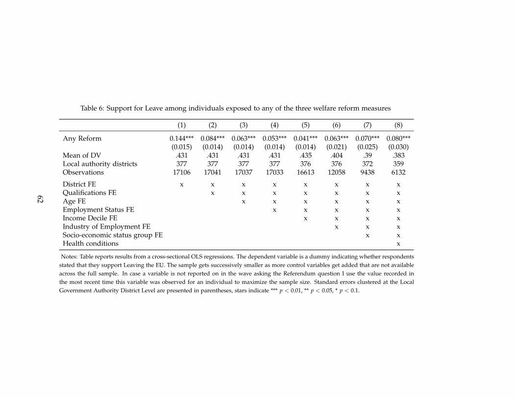
Table 6: Support for Leave among individuals exposed to any of the three welfare reform measures

(1) (2) (3) (4) (5) (6) (7) (8)

Any Reform 0.144*** 0.084*** 0.063*** 0.053*** 0.041*** 0.063*** 0.070*** 0.080***(0.015) (0.014) (0.014) (0.014) (0.014) (0.021) (0.025) (0.030)

Mean of DV .431 .431 .431 .431 .435 .404 .39 .383Local authority districts 377 377 377 377 376 376 372 359Observations 17106 17041 17037 17033 16613 12058 9438 6132

District FE x x x x x x x xQualifications FE x x x x x x xAge FE x x x x x xEmployment Status FE x x x x xIncome Decile FE x x x xIndustry of Employment FE x x xSocio-economic status group FE x xHealth conditions x

Notes: Table reports results from a cross-sectional OLS regressions. The dependent variable is a dummy indicating whether respondentsstated that they support Leaving the EU. The sample gets successively smaller as more control variables get added that are not availableacross the full sample. In case a variable is not reported on in the wave asking the Referendum question I use the value recorded inthe most recent time this variable was observed for an individual to maximize the sample size. Standard errors clustered at the LocalGovernment Authority District Level are presented in parentheses, stars indicate *** p < 0.01, ** p < 0.05, * p < 0.1.

62

Online Appendix

“Did Austerity Cause Brexit?”For Online Publication

Thiemo Fetzer

July 22, 2018

This appendix is subdivided into three sections. Section A presents further ro-

bustness checks and additional results as figures or tables that were omitted from

the main paper due to space constraints. These results are directly referred to in

the main text and discussed in the main body or in footnotes. Section B presents

further descriptions of the underlying data as well as additional background mate-

rials. The relevant sections are referred to in the main text. Section C presents a set

of auxiliary results only indirectly referred to in the main text, they are discussed

in detail in this appendix section.

A Further Robustness Checks and Additional Results

1

Figure A1: Non-parametric effect of austerity on support for UKIP overall and by individual measures studyingWestminster elections.

Panel A: Overall austerity shock Panel B: Council Tax Benefit

Panel C: Disability living allow. Panel D: Bedroom Tax

Notes: The dependent variable is the percentage of votes for UKIP in Westminster elections across the 570 harmonized constituencies in the 2001, 2005, 2010 and 2015Westminster elections. The graph plots point estimates of the interaction between the simulated incidence of the austerity measures and a set of year fixed effects with 2010as omitted year. All regression include constituency fixed effects and NUTS1 region by year fixed effects. Standard errors are clustered at the constituency level with 90%confidence bands indicated.

2

Figure A2: Non-parametric effect of austerity on support for UKIP overall and by individual measures studyingEuropean elections.

Panel A: Overall austerity shock Panel B: Council Tax Benefit

Panel C: Disability living allow. Panel D: Bedroom Tax

Notes: The dependent variable is the percentage of votes for UKIP in European Parliamentary elections of 2004, 2009 and 2014 at the district level. The graph plots pointestimates of the interaction between the simulated incidence of the austerity measures and a set of year fixed effects with 2009 being the omitted year. All regression includedistrict fixed effects and NUTS1 region by year fixed effects. Standard errors are clustered at the district level with 90% confidence bands indicated.

3

Figure A3: Effect of Austerity on Local Area Gross Value Added per capita

Notes: The dependent variable is the log value of the gross value added per working age adult in a local authority areabetween 2000 to 2015. The graph plots point estimates of the interaction between the overall simulated local authority areaausterity incidence and a set of year fixed effects. All regression include local authority district fixed effects and NUTS1region by year fixed effects. Standard errors are clustered at the district level with 90% confidence bands indicated.

4

Figure A4: Support for Leave in EU referendum by respondent’s political partypreference

Notes: The plot presents sample averages of Leave support in Wave 8 of the USOC survey by the respondents expressedpolitical support for UKIP, the Conservatives, Labour or the Liberal Democrats.

5

Figure A5: Excluding individuals ever having worked in manufacturing, mining or agriculture: Non-parametricestimates capturing the evolution of labor and benefit income within individuals over time for respondents with low-and high levels of human capital

Panel A: Evolution of benefit and labor income for individuals with no qualifications

Labor income Benefit income Gross income

Panel B: Evolution of benefit and labor income for individuals with university degree

Labor income Benefit income Gross income

Notes: The dependent variable is the monthly gross labor income on the left, and the monthly benefit income on the right. The population is restricted to the sample of BHPSand USOC respondents that are not retired and that have never worked in manufacturing, mining or agriculture. The BHPS survey waves 11-18 start in 2001 and end in 2009,while the larger USOC survey starts in 2009 and includes some, but not all of the former BHPS from Wave 2 onwards. The graph plots point estimates of the interactionbetween the qualification status of respondents (having no qualifications in top row, versus having a university degree in bottom row) on monthly labor or benefit income.All regression include individual respondent fixed effects and local authority by survey wave by time fixed effects. Standard errors are clustered at the district level with 90%confidence bands indicated.

6

Table A1: Robustness of the Impact of different austerity measures on support for UKIPacross Local, European and Westminster elections: Adding district specific linear timetrends

(1) (2) (3) (4) (5) (6)Overall TC CB CTB DLA BTX

Panel A: Local1(Year>2010) × Austerity 0.005* 0.036*** 0.094** 0.051 0.052* 0.040

(0.002) (0.012) (0.038) (0.034) (0.027) (0.069)Mean of DV 4.49 4.49 4.49 4.49 4.49 4.49Local authority districts 345 346 346 346 346 346Observations 3260 3263 3263 3263 3263 3263

Panel B: European1(Year>2010) × Austerity 0.004 0.030** 0.015 0.025 0.070*** -0.059

(0.003) (0.014) (0.035) (0.038) (0.027) (0.057)Mean of DV 21.1 21.1 21.1 21.1 21.1 21.1Local authority districts 378 379 379 379 379 379Observations 1134 1137 1137 1137 1137 1137

Panel C: Westminster1(Year>2010) × Austerity 0.010*** 0.081*** -0.016 0.073** 0.164*** 0.118**

(0.002) (0.010) (0.031) (0.035) (0.024) (0.051)Mean of DV 6.03 6.03 6.03 6.03 6.03 6.03Harmonized Constituencies 566 566 566 566 566 566Observations 2047 2047 2047 2047 2047 2047

Avg Loss per working age adult 447.1 87.97 71.52 7.21 36.57 10.81Affected HH. in 1000s 4507 7601 2436 499 660Correlation with...

No qualification share .75 .17 .51 .77 .58Routine job share .6 .12 .27 .62 .43Retail sector share .35 .28 .02 .21 .08Manufacturing sector share .3 .11 -.03 .37 .24

Notes: Table reports results from a panel OLS regressions with local authority area and region by year fixedeffects. The dependent variable is UKIP’s vote share in the Local Elections from 2000 to 2015. Standard errorsclustered at the Local Government Authority District Level are presented in parentheses, stars indicate ***p < 0.01, ** p < 0.05, * p < 0.1.

7

Table A2: Effect of austerity on political preferences: Studying the original political prefer-ences of supporters of different political parties

(1) (2) (3) (4) (5)UKIP Conservatives Labour Lib Dems No party

Initial party preference...Conservatives × Post × Any 0.047*** -0.080*** 0.029** 0.008 0.002

(0.013) (0.016) (0.013) (0.007) (0.012)Labour × Post × Any 0.007 -0.026*** 0.021** -0.001 0.000

(0.006) (0.005) (0.010) (0.003) (0.008)Lib Dems × Post × Any 0.045** -0.061*** -0.002 0.006 0.013

(0.018) (0.012) (0.020) (0.019) (0.018)None × Post × Any 0.003 -0.039*** 0.022* -0.006 0.027**

(0.009) (0.007) (0.012) (0.005) (0.014)UKIP × Post × Any 0.006 -0.020 0.007 0.006 -0.000

(0.037) (0.020) (0.022) (0.010) (0.029)Other × Post × Any 0.057*** -0.014 -0.022 -0.013 0.020

(0.020) (0.011) (0.020) (0.010) (0.019)Mean of DV .0479 .263 .351 .082 .187Local authority districts 378 378 378 378 378Observations 231887 231887 231887 231887 231887

Individual FE x x x x xDistrict x Region x Time FE x x x x x

Notes: Table reports results from a panel OLS. The dependent variable is a dummy variable taking thevalue 1 in case a respondent expresses support for the party provided in the column head (either statingthey are a supporter, feel close or would vote for the party if there was a general election tomorrow). Theunderlying regression interacts the individual level exposure to welfare reforms studied in Table 3 with abaseline measure of an individual’s stated political party preference recorded the first time the respondentscontribute to the USOC study. Standard errors clustered at the Local Government Authority District Levelare presented in parentheses, stars indicate *** p < 0.01, ** p < 0.05, * p < 0.1.

8

Table A3: Effect of exposure to welfare cuts on like/ or dislike of the estab-lished political parties: included only in Wave 2, 3 and 6 in USOC study

(1) (2) (3)

Panel A: Like or dislike ConservativesPost × Benefit cut -0.178*** -0.221*** -0.173*

(0.055) (0.059) (0.100)Mean of DV 3.53 3.53 3.53Local election districts 378 378 378Observations 75077 75077 75077

Panel B: Like or dislike LabourPost × Benefit cut -0.020 -0.041 -0.045

(0.061) (0.066) (0.103)Mean of DV 4.09 4.09 4.09Local election districts 378 378 378Observations 75193 75193 75193

Panel C: Like or dislike Liberal DemocratsPost × Benefit cut 0.090* 0.032 -0.015

(0.050) (0.053) (0.097)Mean of DV 3.07 3.07 3.07Local election districts 378 378 378Observations 73783 73783 73783

District FE ×Region x Wave x Time FE ×District x Wave x Time FE × ×Individual FE ×

Notes: Table reports results from a OLS regressions. The dependent variable capturethe extent to which respondents like or dislike one of the three main political parties.They are measured on a 10 point Likert scale ranging from strong dislike to strongly like.Standard errors clustered at the Local Government Authority District Level are presentedin parentheses, stars indicate *** p < 0.01, ** p < 0.05, * p < 0.1.

9

Table A4: Alternative broader outcome measures and support for Leave across different control variables

(1) (2) (3) (4) (5) (6) (7) (8)

My vote doesnt matter 0.001 0.009 0.014 0.014 0.014 0.014 0.012 0.014(0.010) (0.009) (0.009) (0.009) (0.009) (0.011) (0.012) (0.015)

Public officials dont care 0.052*** 0.041*** 0.037*** 0.037*** 0.035*** 0.036*** 0.028*** 0.034***(0.006) (0.006) (0.006) (0.006) (0.006) (0.007) (0.007) (0.009)

Dont have a say in what govt does 0.043*** 0.032*** 0.032*** 0.032*** 0.031*** 0.027*** 0.027*** 0.029***(0.005) (0.005) (0.005) (0.005) (0.005) (0.006) (0.006) (0.008)

Mean of DV .438 .438 .438 .438 .438 .403 .388 .386Local authority districts 374 374 374 374 374 373 369 344Observations 12709 12674 12670 12667 12667 9276 7232 4495

District FE x x x x x x x xQualifications FE x x x x x x xAge FE x x x x x xEmployment Status FE x x x x xIncome Decile FE x x x xIndustry of Employment FE x x xSocio-economic status group FE x xHealth conditions x

Notes: Table reports results from a cross-sectional OLS regressions. The dependent variable is a dummy indicating whether respondentsstated that they support Leaving the EU. The sample gets successively smaller as more control variables get added that are not availableacross the full sample. In case a variable is not reported on in a specific wave, the most recent time a control variable is observed for anindividual in the panel is used. Standard errors clustered at the Local Government Authority District Level are presented in parentheses,stars indicate *** p < 0.01, ** p < 0.05, * p < 0.1.

10

B Data and Additional Background Material

B.1 Validating the use of UKIP vote shares to capture anti-EU

sentiment

One might be worried that UKIP vote shares in EP elections are not measuring

anti-EU sentiments but potentially other dimensions of political preferences. Micro

data from the British Election Study (BES) me to see whether support for UKIP is

strongly associated with support for Leave.

The BES surveys are carried out with prospective voters from sampled wards

across a (changing) sample of roughly 200 Westminster parliamentary constituen-

cies. The sampling is not representative at the local authority district level and it is

not guaranteed that the same constituencies or the same wards are sampled across

different rounds, which makes it econometrically less appealing to work with this

data. The survey is usually carried out reliably around British general elections.

Appendix Table B1 shows that self-reported individual (planned) voting for

UKIP in the British general elections in 2005, 2010 and 2015 is a meaningful indi-

cator for anti-EU and anti-immigration preferences across a range of these cross

sections. In particular, the analysis suggests that UKIP voters are more likely to

support the view that the EU is responsible for the UK’s debt levels, that the EU

is a threat to British sovereignty, that Britain let in too many immigrants into the

country and that immigration increases crime, is bad for the economy and for job

prospects of natives.

B.2 Council elections

The data for district elections in Great Britain is taken from The Elections Cen-

tre. It contains comprehensive data on local government elections since 1973. Since

1999, there have been several changes in local government structure, and these

have been accounted for in constructing the panel.

The current local government structure includes both two-tier and single-tier

components. In England, there are 27 upper-tier county councils with 201 lower-

tier district councils. Additionally, there are 32 London Boroughs, the City of Lon-

11

Table B1: Validation of UKIP vote as measure of anti-EU and anti immigration sentiment

(1) (2) (3)

Panel A: (Strongly) disapprove of British EU membership [2005, 2010, 2015]

(Will) vote for UKIP 0.450*** 0.457*** 0.460***(0.030) (0.031) (0.033)

Mean of DV .331 .345 .352LGA Districts 270 226 198Respondents 7295 4958 4440

Panel B: (Strongly) agree EU is responsible for UK debt [2015]

(Will) vote for UKIP 0.138*** 0.142*** 0.158***(0.034) (0.036) (0.037)

Mean of DV .265 .276 .286LGA Districts 209 181 155Respondents 2019 1718 1519

Panel C: (Strongly) disagree that EU threat to British sovereignty is exaggerated [2005]

(Will) vote for UKIP 0.324*** 0.312*** 0.253**(0.080) (0.101) (0.117)

Mean of DV .31 .327 .326LGA Districts 104 69 59Respondents 4296 2454 2204

Panel C: Immigration is not good for economy [2005, 2010]

(Will) vote for UKIP 0.396*** 0.356** 0.355*(0.147) (0.172) (0.184)

Mean of DV 3.03 3.04 3.07LGA Districts 191 147 128Respondents 4702 2975 2689

Panel C: Immigrants take jobs from natives [2005, 2010]

(Will) vote for UKIP 0.447*** 0.453** 0.382**(0.151) (0.189) (0.175)

Mean of DV 3.03 3.06 3.08LGA Districts 190 146 127Respondents 5096 3104 2795

Panel D: Yes, too many immigrants have been let into this country [2015](Will) vote for UKIP 0.255*** 0.258*** 0.254***

(0.016) (0.016) (0.015)Mean of DV .73 .731 .751LGA Districts 209 181 155Respondents 2019 1718 1519

Panel E: (Strongly) agree immigrants increase crime rates [2005, 2010](Will) vote for UKIP 0.293*** 0.275*** 0.260***

(0.061) (0.071) (0.075)Mean of DV .44 .462 .468LGA Districts 191 147 128Respondents 4690 2963 2677

Sample All England Not LondonRespondent controls Yes Yes YesRegion x Year FE Yes Yes Yes

Notes: Table reports results from a OLS regressions on variables obtained from the 2005, 2010 and 2015 British Election Study. The years in whichdata is available for respective question is presented in parenthesis. All regressions control for respondent age, gender, an indicator of whether therespondent has no formal qualifications, a quadratic in age and an interaction with the education indicator and age. Standard errors clustered at theLocal Government Authority District Level are presented in parentheses, stars indicate *** p < 0.01, ** p < 0.05, * p < 0.1.

12

don, 36 metropolitan boroughs (or districts), and 55 unitary authorities (UA), all

of which operate on a single-tier basis. Since 1994, there are 22 unitary authorities

in Wales and 32 unitary authorities in Scotland. While most responsibilities are

split between counties and districts in two-tier authorities, single-tier authorities

must provide all the services . In constructing the sample, this paper includes all

election results at the district council and single-tier authority level between 2000

and 2015.

Elections are organized by subdivisions of local authorities called electoral

wards or electoral divisions. Each ward is represented by one or more elected

councilors. Although in all cases councilors serve 4 year terms, there are three

distinct systems of elections. First, elections may happen every four years for all

councilors. Second, elections may happen for a third of the councilors every year,

with no election in the fourth year. In this case, the fourth year is used for county

council elections. Third, half of the councilors may be elected every two years .

In terms of voting system, England and Wales use First Past the Post, while the

Single Transferable Vote system is used in Scotland and Northern Ireland. In the

analysis, a system of elections every four years starting in 2000 is treated separately

from a system with elections every four years starting in 2000. Thus, all additional

variation is taken into account with “election wave” fixed effects, which control for

differences between authorities with different elections structures and sequences.

The main change in the structure of local government since 2000 was the in-

troduction of nine new unitary authorities in England in 2009. These changes

are summarized in the table below. In the first five county councils, the lower

tier district councils were abolished, and all functions were undertaken by the new

unitary authority of the same name. In Bedfordshire, Mid- and South Bedfordshire

merged to form the Central Bedfordshire UA. Bedford attained UA status, having

previously been a district. In Cheshire, the unitary authority of Cheshire West and

Chester was formed from the districts of Ellesmere Port and Neston, Vale Royal,

and Chester. The districts of Macclesfield, Congleton and Crewe and Nantwich

merged to form Cheshire East. In order to compare the regions before and after

these reforms, district-level results were merged into the current UA boundaries

13

between 2000 and 2008. There is no concern of overlap, as no district council was

split to form the new unitary authorities.

Table B2: Changes to district councils since 2000

County Council (before 2009) District Councils New Unitary Authority (After 2009)

(Before 2009)Cornwall Caradon Cornwall

CarrickKerrierNorth CornwallPenwithRestormel

Durham Cheshire-le-Street DurhamCity of DurhamDerwentsideEasingtonSedgefieldTeesideWear Valley

Northumberland Alnwick NorthumberlandBerwick-upon-TweedBlyth ValleyCastle MorpethTynedaleWansbeck

Shropshire Bridgnorth ShropshireNorth ShropshireOswestryShrewsbury and AtchamSouth Shropshire

Wiltshire Kennet WiltshireNorth WiltshireSalisburyWest Wiltshire

Bedfordshire Mid Bedfordshire BedfordSouth Bedfordshire Central Bedfordshire

Cheshire Chester Cheshire West and ChesterCongleton Cheshire EastCrewe and NantwichEllesmere Port and NestonMacclesfieldVale Royal

B.3 Political preferences elicited through the USOC survey

The key value added of working with individual level panel data lies in the fact

that I can fully zoom in on changes in political preferences within an individual.

The instrument used for each USOC survey round contains a Politics module that

14

elicits political preferences through a sequence of questions. These are presented

in Figure B1. The enumerator asks the respondents first, whether an individual is a

supporter of a political party. If the respondent says yes, they enquire which is the

political party. In case respondents said that they are not a supporter of a specific

party, the enumerator asks whether the respondent sees him- or herself closer to

one party or another. If that is the case, the enumerator asks, which political party

that is.

Only if a respondent is neither a supporter of a political party or feeling closer

to one party over another one, the enumerator asks, which party would the re-

spondent vote for in case there was an election.

In the face-to-face interviews, respondents are not directly prompted with party

names from a menu, but rather respondents are asked to provide the party name,

which the enumerator ticks on the survey questionnaire or, alternatively, details.

In waves 1-3, the conversion of the survey questionnaires (containing the detailed

party names) to digital files, did not separately code UKIP, but rather, included

a broad category ”Other” – the other main parties, in particular, Labour, Conser-

vatives, Liberal Democrats, Greens, Plaid Cymru, Scottish Nationalists as well as

Sinn Fein for Northern Ireland are always consistently coded.

Conversations with the UK Data Service handling the USOC data confirms

that most of the Other-coded responses prior to wave 3 were supporters of UKIP

or the British Nationalist Party (BNP). From Wave 4 onwards, UKIP is separately

coded and the pool of respondents in the maintained ”Other” category collapses

once UKIP is separately coded. To be consistent throughout, I include the Other

category into the count of UKIP supporters from Wave 4 onwards as well, which

likely adds some noise to the dependent variable.

This narrow module is complemented with a more detailed Political engagement

module in wave 2, 3 and 6. The political engagement module includes six further

survey questions explored in this paper.

• ”Public officials don’t care” – respondents are asked to (strongly) disagree or

(strongly) agree with this statement on a 5 point Likert scale.

• ”I don’t have a say in what the government does” – respondents are asked to

15

(strongly) disagree or (strongly) agree with this statement on a 5 point Likert

scale.

• Perceived political influence – respondents are asked “On a scale from 0 to

10, where 0 means very unlikely and 10 means very likely, how likely is

it that your vote will make a difference in terms of which party wins the

election in this constituency at the next general election?” – in this paper I

code respondents reporting are score weakly lower than 3 as perceiving that

their vote is unlikely to make a difference.

• Party likes- and dislikes – respondents are asked for each of the three main

parties (Conservative/Labour/ Liberal Democrats) ”On a scale from 0 to 10,

where 0 means strongly dislike and 10 means strongly like, how do you feel

about the ... Party ?”

16

Figure B1: Schematic of USOC survey instrument eliciting political party prefer-ences

Notes: Schematic presenting the structure of the USOC survey instrument eliciting political party preferences of individualrespondent.

17

C Auxiliary Results

C.1 Robustness of trend changes in UKIP support

In this appendix, I present a range of robustness checks to highlight that the

trends presented in Section 3 are robust.

Similar trends for EP and Westminster elections While the trends presented in

the main paper focus on the local elections, due to the high frequency of election

results data for local elections, the trend patterns are very similar when studying

EP or Westminster elections. Appendix Figure C1 shows that the marked change

in the correlation structure between UKIP support and measures of poor economic

fundamentals of 2001 constituency boundaries harmonized constituencies are very

similar, with UKIP support picking up markedly in areas with high shares of the

local population with No Qualifications, working in Routine jobs or high shares

of Retail- and Manufacturing sector employment. The same patterns appear when

studying EP elections as evidenced in Figure C2. While, on average, UKIP vote

shares in Local and Westminster elections are mechanically lower (as not all seats

are contested), UKIPs performance in EP elections 2004, 2009 and 2014 stands out

consistently realizing more than 15.6% of the vote.

Functional form The set of fixed effects included in the main specification is

quite demanding. The results are very similar if I control fo more or less demand-

ing time-fixed effects. In particular, Appendix Figures C10 show the estimated

coefficients, when controlling for election-wave by region and year fixed effects.

This set of fixed effects is particularly suitable as it de-facto zooms in on districts

that are on similar rotation schedules for the elections of councillors. Similarly,

Appendix Figure C11) presents results using simple year fixed effects; throughout,

the results patterns are very similar.

Sample balance UKIP does not field candidates in each of the local council elec-

tions. In the overall panel, UKIP is coded has having zero percentage of votes

in case it does not field candidates. The results are however, robust to focusing

on a much more balanced panel, including only districts in which UKIP fielded

18

candidates in at least 50% of the elections. These results are presented in Figure

C9, the trends remain very similar. This, taken together with the similar trends

we document for the EP (where candidates are fielded throughout the UK as they

are selected based on the party’s performance in regional lists) and Westminster

elections renders me confident that the results are not masking selection effects.

Broader baseline categories or measures The presentation of trends in Section

3 is condensed to a small set of baseline characteristics Xi,baseline. In this section,

I show that the results are robust to a much richer set of baseline characteristics.

In particular, Appendix Figure C5 shows a richer set of plots for six distinct qual-

ification groups; the increase in support for UKIP is driven by areas that have a

relatively low skill composition of the local resident population, while the reverse

is true for areas with a resident population with higher degrees.

Appendix Figure C6 shows a richer set of plots for the eight distinct socio-

economic status groups that the UK census bureau distinguishes. The Census

bureau categorizes individual occupations and job titles into these socio-economic

status groups, following the Goldthorpe classification system from sociology.

Appendix Figure C7 presents a broader set of sectors, suggesting that no trend

patterns emerge for areas that have a sizable Health Care or Hotel & Accommoda-

tion sector. Similar positive effects on UKIP are found for the Transportation and

Construction sectors, while the opposite direction shows up for Education and

Real Estate.

In particular, I use refined baseline measures focusing on the qualification pro-

file of the UK-born resident population (as opposed to including foreign borns).

This exercise serves to zoom in on the likely electorate, which is mostly drawn

from the UK-born resident population, despite EU citizens being entitled to vote

in local elections. These results are presented in Appendix Figure C12 and provide

very similar patterns.

C.2 Where do UKIP voters come from?

The EU referendum was announced in early 2013 by the Conservative Prime

Minister David Cameron, on condition of winning a majority in the 2015 election.

This suggests that UKIP was particularly perceived as a threat to the Conservative

19

party.

Yet, the previous literature suggests that UKIP also attracted supporters from

the Labour party. Similarly, it could be that UKIP was particularly successful in

mobilizing voters that previously did not turn out to vote in elections.

I investigate these in turn.

Empirical specification I build on our previous analysis that documents that

UKIP’s electoral ascent post 2010 is driven by places with weak economic funda-

mentals. I now ask whether these fundamentals, after 2010, explain distinct moves

away from other parties by estimating the following specification

yirt = αi + βrt + γ× Post 2010× Xi,baseline + εirt (7)

The only difference to the previous specification is that now, we explore a range

of dependent variables yirt. In addition to the UKIP vote shares, we present results

pertaining to turnout, the Conservative-, Labour- and Liberal Democrat party vote

shares. Furthermore, due to space constraints, we present not the full sequence of

non-parametric effects, but rather, focus on a pooled average post 2010 coefficient

estimate γ to be presented in table form.

I perform the analysis at the level of local council elections, European Parlia-

mentary elections as well as Westminster elections.

Results The results pertaining to the study of local elections are presented in

Table C1. The results suggest that UKIP’s growth that is captured by the weak

baseline socio-economic characteristics comes mostly at the expense of Conserva-

tive party vote shares as indicated by the negative coefficients in column (3) across

most proxy measures for weak-socio economic fundamentals, with the exception

of the share of residents working in retail.

There is no statistically discernible effect on turnout, suggesting that places

with weak socio-economic fundamentals post 2010 saw no differential voter mo-

bilization from which UKIP could have benefited. If anything, the point estimates

are negative throughout.

This analysis suggests that the Conservative party, in local elections, was losing

non-negligible numbers of voters to UKIP. This is not surprising, as Conservative

20

councillors defected to UKIP quite regularly (Webb and Bale, 2014).

I obtain very similar results when studying the performance of UKIP and the

other parties in the European Parliamentary election of 2014 (relative to the earlier

rounds) and the 2015 Westminster election (relative to the 2001, 2005 and 2010

elections). These results are presented in Appendix Tables C2 and C3.

On the timing Since the EU referendum was already announced in January 2013,

it becomes interesting to see whether the link between weak socio-economic funda-

mentals and UKIP votes is already present in the data prior to the announcement,

in particular up to the 2012 local council elections that were held in May 2012.

I restrict the analysis to the two local election rounds in 2011 and 2012 and

present the results in Table C4. The pattern is similar, but also suggests some

distinct differences. We find the same positive link between weak socio-economic

fundamentals and UKIP votes after 2010. It is statistically significant for two of the

four indicators of weak socio-economic fundamentals: for the share of the resident

population with low qualification and for the prevalence of retail employment.

There are some differences in the effects on other parties: while the Conserva-

tive party appears to be contracting in such areas, the Labour party, along with

UKIP actually stands to gain. This suggests that prior to the EU referendum an-

nouncement, in local elections, a growing support for UKIP is associated with a

worse performance for the Conservatives and a better performance for Labour in

areas with weak fundamentals, suggesting that the perceived threat of UKIP, in-

creasing the risk of a shift towards Labour may have been particularly strongly

perceived in the run up to the January 2013 announcement.

21

Figure C1: Non-parametric effect of educational qualification, socio-economic status, and sectoral employment ofthe resident population as of 2001 on support for UKIP in Westminster Parliamentary elections from 2001 - 2015 overtime

Panel A: No qualifications Panel B: Routine jobs

Panel C: Retail Panel D: Manufacturing

Notes: The dependent variable is the percentage of votes for UKIP in Westminster elections at the harmonized 2010 constituency level. Panel A uses the share of the residentpopulation with no formal qualifications as of 2001. Panel B uses the share of the resident population in Routine jobs as per the National Socio-Economic Classification ofOccupations as of 2001. Panel C uses the share of the resident working age population employed in the Retail sector, while panel D uses the share of the resident workingage population employed in Manufacturing. The graph plots point estimates of the interaction between these cross sectional measures and a set of year fixed effects. Allregression include local authority district fixed effects and election wave by NUTS1 region by year fixed effects. Standard errors are clustered at the district level with 90%confidence bands indicated.

22

Figure C2: Non-parametric effect of educational qualification, socio-economic status, and sectoral employment ofthe resident population as of 2001 on support for UKIP in European Parliamentary elections over time

Panel A: No qualifications Panel B: Routine jobs

Panel C: Retail Panel D: Manufacturing

Notes: The dependent variable is the percentage of votes for UKIP in European Parliamentary elections at the local authority district level. Panel A uses the share of theresident population with no formal qualifications as of 2001. Panel B uses the share of the resident population in Routine jobs as per the National Socio-Economic Classificationof Occupations as of 2001. Panel C uses the share of the resident working age population employed in the Retail sector, while panel D uses the share of the resident workingage population employed in Manufacturing. The graph plots point estimates of the interaction between these cross sectional measures and a set of year fixed effects. Allregression include local authority district fixed effects and election wave by NUTS1 region by year fixed effects. Standard errors are clustered at the district level with 90%confidence bands indicated.

23

Figure C3: Non-parametric effect of educational qualification of the resident population in 2001 on support for UKIPover time

Panel A: Other qualifications Panel B: No Qualification Panel C: Level 1

Panel D: Level 2 Panel E: Level 3 Panel F: Level 4 plus

Notes: The variable is the respective share of the resident population in a local authority district that has obtained the educational qualifications following the UK classificationsystem, whereby No qualifications means no formal qualification or school leaving certificate, Level 1 stands for having between 1-4 General Certificate of Secondary Education(GCSE) qualifications, Level 2 stands for 5 GCSEs, Level 3 means having 2 or more A-levels (university qualifying), while level 4 or above captures having a university degree.Other qualifications includes apprenticeships and foreign qualification below a university degree. The graph plots point estimates of the interaction between these crosssectional measures and a set of year fixed effects. All regression include local authority district fixed effects and NUTS1 region by year fixed effects. Standard errors areclustered at the district level with 90% confidence bands indicated.

24

Figure C4: Non-parametric effect of socio-economic employment status of the resident population in 2001 on supportfor UKIP over time

Panel A: Long term unemployed Panel B : Routine job Panel C: Semi-routine Panel D: Lower supervisory

Panel E: Student Panel F: Lower management Panel G: Higher professional Panel H: Higher management

Notes: The variable is the respective share of the resident population in a district that is in either socio-economic status classification as of 2001. The graph plots pointestimates of the interaction between these cross sectional measures and a set of year fixed effects. All regression include local authority district fixed effects and NUTS1 regionby year fixed effects. Standard errors are clustered at the district level with 90% confidence bands indicated.

25

Figure C5: Non-parametric effect of educational qualification of the resident population in 2001 on support for UKIPover time

Panel A: Other qualifications Panel B: No Qualification Panel C: Level 1

Panel D: Level 2 Panel E: Level 3 Panel F: Level 4 plus

Notes: The variable is the respective share of the resident population in a local authority district that has obtained the educational qualifications following the UK classificationsystem, whereby No qualifications means no formal qualification or school leaving certificate, Level 1 stands for having between 1-4 General Certificate of Secondary Education(GCSE) qualifications, Level 2 stands for 5 GCSEs, Level 3 means having 2 or more A-levels (university qualifying), while level 4 or above captures having a university degree.Other qualifications includes apprenticeships and foreign qualification below a university degree. The graph plots point estimates of the interaction between these crosssectional measures and a set of year fixed effects. All regression include local authority district fixed effects and NUTS1 region by year fixed effects. Standard errors areclustered at the district level with 90% confidence bands indicated.

26

Figure C6: Non-parametric effect of socio-economic employment status of the resident population in 2001 on supportfor UKIP over time

Panel A: Long term unemployed Panel B : Routine job Panel C: Semi-routine Panel D: Lower supervisory

Panel E: Student Panel F: Lower management Panel G: Higher professional Panel H: Higher management

Notes: The variable is the respective share of the resident population in a district that is in either socio-economic status classification as of 2001. The graph plots pointestimates of the interaction between these cross sectional measures and a set of year fixed effects. All regression include local authority district fixed effects and NUTS1 regionby year fixed effects. Standard errors are clustered at the district level with 90% confidence bands indicated.

27

Figure C7: Non-parametric effect of the industry employment structure in 2001 onsupport for UKIP over time

Panel A: Education Panel B: Real Estate

Panel C: Retail Panel D: Transport

Panel E: Construction Panel F: Manufacturing

Panel G: Hotel & Accommodation Panel H: Health care

Notes: The dependent variable is the percentage of votes for UKIP in local council elections. The independent variables arethe respective shares of the resident working age population in a district that is working in any of the different sectors as of2001 interacted with a set of year fixed effects. All regression include local authority district fixed effects and NUTS1 regionby year fixed effects. Standard errors are clustered at the district level with 90% confidence bands indicated.

28

Figure C8: Non-linear time trend in support for UKIP after partialing out non-lineartrend in baseline manufacturing sector prevalence and import-shock

Panel A: No qualifications Panel B: Routine jobs

Panel C: Retail

Notes: The dependent variable is the percentage of votes for UKIP in local council elections. Panel A uses the share ofthe resident UK born population with no formal qualifications as of 2001. Panel B uses the share of the UK born residentpopulation in Routine jobs as per the National Socio-Economic Classification of Occupations as of 2001. The graph plotspoint estimates of the interaction between these two cross sectional measures and a set of year fixed effects. All regressioninclude local authority district fixed effects and NUTS1 region by year fixed effects, in addition to year effects interactedwith the baseline size of the manufacturing sector in terms of employment as of 2001. Standard errors are clustered at thedistrict level with 90% confidence bands indicated.

29

Figure C9: Robustness to balanced sample of elections – Non-parametric effect ofeducational qualification, socio-economic status, and sectoral employment of theresident population as of 2001 on support for UKIP over time

Panel A: No qualifications Panel B: Routine jobs

Panel C: Retail Panel D: Manufacturing

Notes: The dependent variable is the percentage of votes for UKIP in local council elections. The sample is restricted toonly include elections where UKIP ran across districts in which UKIP contested at least 50% of the races. Panel A uses theshare of the resident population with no formal qualifications as of 2001. Panel B uses the share of the resident populationin Routine jobs as per the National Socio-Economic Classification of Occupations as of 2001. Panel C uses the share of theresident working age population employed in the Retail sector, while panel D uses the share of the resident working agepopulation employed in Manufacturing. The graph plots point estimates of the interaction between these cross sectionalmeasures and a set of year fixed effects. All regression include local authority district fixed effects and election wave byNUTS1 region by year fixed effects. Standard errors are clustered at the district level with 90% confidence bands indicated.

30

Figure C10: Robustness to controlling for more demanding time effects: Electionwave by Region by Year – Non-parametric effect of educational qualification, socio-economic status, and sectoral employment of the resident population as of 2001 onsupport for UKIP over time

Panel A: No qualifications Panel B: Routine jobs

Panel C: Retail Panel D: Manufacturing

Notes: The dependent variable is the percentage of votes for UKIP in local council elections. Panel A uses the share of theresident population with no formal qualifications as of 2001. Panel B uses the share of the resident population in Routinejobs as per the National Socio-Economic Classification of Occupations as of 2001. Panel C uses the share of the residentworking age population employed in the Retail sector, while panel D uses the share of the resident working age populationemployed in Manufacturing. The graph plots point estimates of the interaction between these cross sectional measures anda set of year fixed effects. All regression include local authority district fixed effects and election wave by NUTS1 region byyear fixed effects. Standard errors are clustered at the district level with 90% confidence bands indicated.

31

Figure C11: Robustness to controlling for less demanding time effects: Year FE– Non-parametric effect of educational qualification, socio-economic status, andsectoral employment of the resident population as of 2001 on support for UKIPover time

Panel A: No qualifications Panel B: Routine jobs

Panel C: Retail Panel D: Manufacturing

Notes: The dependent variable is the percentage of votes for UKIP in local council elections. Panel A uses the share of theresident population with no formal qualifications as of 2001. Panel B uses the share of the resident population in Routinejobs as per the National Socio-Economic Classification of Occupations as of 2001. Panel C uses the share of the residentworking age population employed in the Retail sector, while panel D uses the share of the resident working age populationemployed in Manufacturing. The graph plots point estimates of the interaction between these cross sectional measures anda set of year fixed effects. All regression include local authority district fixed effects and year fixed effects. Standard errorsare clustered at the district level with 90% confidence bands indicated.

32

Figure C12: Robustness to measurement of baseline characteristics - Focusing onUK born population shares – Non-parametric effect of educational qualification,socio-economic status, and sectoral employment of the resident population as of2001 on support for UKIP over time

Panel A: No qualifications Panel B: Routine jobs

Panel C: Retail Panel D: Manufacturing

Notes: The dependent variable is the percentage of votes for UKIP in local council elections. Panel A uses the share ofthe UK born resident population with no formal qualifications as of 2001. Panel B uses the share of the UK born residentpopulation in Routine jobs as per the National Socio-Economic Classification of Occupations as of 2001. Panel C uses theshare of the UK born resident working age population employed in the Retail sector, while panel D uses the share of theUK born resident working age population employed in Manufacturing. The graph plots point estimates of the interactionbetween these cross sectional measures and a set of year fixed effects. All regression include local authority district fixedeffects and NUTS1 region by year fixed effects. Standard errors are clustered at the district level with 90% confidence bandsindicated.

33

Table C1: Where do UKIP voters post 2010 come from? Studying local elections

Other parties

UKIP Turnout Con Lab LD(1) (2) (3) (4) (5)

Panel A: No qualificationsPost 2010 x Pop. share with No qualifications (2001) 42.746*** -2.326 -25.067*** -0.226 -3.668

(5.257) (4.373) (5.432) (6.508) (6.392)Local election districts 345 345 345 345 345Observations 3259 3258 3259 3259 3259

Panel B: Routine jobsPost 2010 x Working age Pop share working in Routine occupations (2001) 70.572*** -8.372 -37.275*** -15.666 19.746

(11.375) (8.452) (11.182) (12.075) (13.700)Local election districts 345 345 345 345 345Observations 3259 3258 3259 3259 3259

Panel C: RetailPost 2010 x Working age Pop share working in Retail (2001) 109.098*** -3.445 -41.989*** -36.801** 25.956

(13.794) (8.552) (11.774) (16.580) (16.126)Local election districts 345 345 345 345 345Observations 3259 3258 3259 3259 3259

Panel D: ManufacturingPost 2010 x Working age Pop share working in Manufacturing (2001) 24.164*** -7.087 -7.246 -2.400 18.796*

(6.398) (5.710) (7.592) (8.012) (9.786)Local election districts 345 345 345 345 345Observations 3259 3258 3259 3259 3259

Notes: All regressions control for local authority district and NUTS1 region by time fixed effects. Standard errors are adjusted clustering at the local authoritydistrict level with stars indicating *** p < 0.01, ** p < 0.05, * p < 0.1.

34

Table C2: Where do UKIP voters post 2010 come from? Studying European Parliamentary elections

Other parties

UKIP Turnout Con Lab LD(1) (2) (3) (4) (5)

Panel A: No qualificationsPost 2010 x Pop. share with No qualifications (2001) 0.363*** 0.167*** -0.166*** 0.180*** 0.000

(0.041) (0.032) (0.025) (0.048) (0.023)Mean of DV .224 .369 .282 .191 .116Local election districts 346 346 346 346 346Observations 1038 1038 1038 1038 1038

Panel B: Routine jobsPost 2010 x Working age Pop share working in Routine occupations (2001) 0.731*** 0.294*** -0.255*** 0.213** 0.050

(0.078) (0.062) (0.051) (0.083) (0.043)Mean of DV .224 .369 .282 .191 .116Local election districts 346 346 346 346 346Observations 1038 1038 1038 1038 1038

Panel C: RetailPost 2010 x Working age Pop share working in Retail (2001) 0.779*** 0.268*** -0.322*** 0.067 0.079

(0.116) (0.095) (0.064) (0.131) (0.061)Mean of DV .224 .369 .282 .191 .116Local election districts 346 346 346 346 346Observations 1038 1038 1038 1038 1038

Panel D: ManufacturingPost 2010 x Working age Pop share working in Manufacturing (2001) 0.295*** 0.019 -0.020 0.067 0.019

(0.044) (0.046) (0.029) (0.055) (0.035)Mean of DV .224 .369 .282 .191 .116Local election districts 346 346 346 346 346Observations 1038 1038 1038 1038 1038

Notes: All regressions control for state by time fixed effects and local government area (LGA) fixed effects. Standard errors are adjusted for two wayclustering by time and LGA with stars indicating *** p < 0.01, ** p < 0.05, * p < 0.1.

35

Table C3: Where do UKIP voters post 2010 come from? Studying Westminster Parliamentary elections

Other parties

UKIP Turnout Con Lab LD(1) (2) (3) (4) (5)

Panel A: No qualificationsPost 2010 x Pop. share with no qualifications 44.816*** -5.424** -28.815*** -8.743** 15.998***

(3.006) (2.129) (2.974) (4.069) (3.295)Mean of DV 6.03 62.9 35.9 35.8 18.1Harmonized constituencies 566 573 573 573 573Observations 2047 2285 2283 2283 2283

Panel B: Routine jobsPost 2010 x Working age pop. share working in routine occupations 96.878*** -29.340*** -27.619*** -58.484*** 26.620***

(5.396) (3.607) (6.600) (7.960) (6.591)Mean of DV 6.03 62.9 35.9 35.8 18.1Harmonized constituencies 566 573 573 573 573Observations 2047 2285 2283 2283 2283

Panel C: RetailPost 2010 x Working age pop. share working in Retail 105.018*** -35.603*** -15.902* -81.719*** 23.520**

(10.381) (4.952) (8.871) (11.848) (9.592)Mean of DV 6.03 62.9 35.9 35.8 18.1Harmonized constituencies 566 573 573 573 573Observations 2047 2285 2283 2283 2283

Panel D: ManufacturingPost 2010 x Working age pop. share working in Manufacturing 42.112*** -20.545*** -1.271 -36.274*** 15.915***

(3.323) (2.020) (3.965) (4.718) (3.723)Mean of DV 6.03 62.9 35.9 35.8 18.1Harmonized constituencies 566 573 573 573 573Observations 2047 2285 2283 2283 2283

Notes: All regressions control for state by time fixed effects and local government area (LGA) fixed effects. Standard errors are adjusted for two wayclustering by time and LGA with stars indicating *** p < 0.01, ** p < 0.05, * p < 0.1.

36

Table C4: Where do UKIP voters post 2010 come from? Studying local elections prior to 2013

Other parties

UKIP Turnout Con Lab LD(1) (2) (3) (4) (5)

Panel A: No qualificationsPost 2010 x Pop. share with No qualifications (2001) 9.630** -6.431 -21.595*** 23.928*** -6.244

(3.802) (4.616) (6.029) (7.328) (6.646)Local election districts 345 345 345 345 345Observations 2612 2612 2612 2612 2612

Panel B: Routine jobsPost 2010 x Working age Pop share working in Routine occupations (2001) 9.723 -15.657* -30.527** 35.622*** 9.399

(7.610) (8.801) (12.041) (13.635) (13.934)Local election districts 345 345 345 345 345Observations 2612 2612 2612 2612 2612

Panel C: RetailPost 2010 x Working age Pop share working in Retail (2001) 30.152*** -10.296 -17.581 11.671 17.527

(10.990) (8.616) (12.753) (20.722) (16.993)Local election districts 345 345 345 345 345Observations 2612 2612 2612 2612 2612

Panel D: ManufacturingPost 2010 x Working age Pop share working in Manufacturing (2001) 2.378 -4.348 0.212 17.115** 12.985

(3.454) (5.329) (7.044) (8.480) (9.530)Local election districts 345 345 345 345 345Observations 2612 2612 2612 2612 2612

Notes: All regressions control for local authority district and NUTS1 region by time fixed effects. Standard errors are adjusted clustering at the local authoritydistrict level with stars indicating *** p < 0.01, ** p < 0.05, * p < 0.1.

37