Discussion PaPer series

IZA DP No. 10610

Sungjin ChoJihye KamSoohyung Lee

Efficient Supply of Human Capital:Role of College Major

mArch 2017

Any opinions expressed in this paper are those of the author(s) and not those of IZA. Research published in this series may include views on policy, but IZA takes no institutional policy positions. The IZA research network is committed to the IZA Guiding Principles of Research Integrity.The IZA Institute of Labor Economics is an independent economic research institute that conducts research in labor economics and offers evidence-based policy advice on labor market issues. Supported by the Deutsche Post Foundation, IZA runs the world’s largest network of economists, whose research aims to provide answers to the global labor market challenges of our time. Our key objective is to build bridges between academic research, policymakers and society.IZA Discussion Papers often represent preliminary work and are circulated to encourage discussion. Citation of such a paper should account for its provisional character. A revised version may be available directly from the author.

Schaumburg-Lippe-Straße 5–953113 Bonn, Germany

Phone: +49-228-3894-0Email: publications@iza.org www.iza.org

IZA – Institute of Labor Economics

Discussion PaPer series

IZA DP No. 10610

Efficient Supply of Human Capital:Role of College Major

mArch 2017

Sungjin ChoSeoul National University

Jihye KamUniversity of Wisconsin, Madison

Soohyung LeeSogang University, University of Maryland, IZA and MPRC

AbstrAct

IZA DP No. 10610 mArch 2017

Efficient Supply of Human Capital:Role of College Major*

This study examines the extent to which changing the composition of college majors

among working-age population may affect the supply of human capital or effective labor

supply. We use the South Korean setting, in which the population is rapidly aging, but

where, despite their high educational attainment, women and young adults are still weakly

attached to the labor market. We find that Engineering majors have an advantage in

various outcomes such as likelihood of being in the labor force, being employed, obtaining

long-term position, and earnings, while Humanities and Arts/Athletics majors show the

worst outcomes. We then conduct a back-of-the-envelope calculation of the impact of the

recently proposed policy change to increase the share of Engineering majors by 10 percent

starting in 2017. Our calculation suggests that the policy change may have a positive but

small impact on labor market outcomes.

JEL Classification: I2, J2, J4

Keywords: economics of education, college major, returns to schooling, gender gap, human capital, aging

Corresponding author:Soohyung LeeDepartment of EconomicsUniversity of Maryland3114 Tydings HallCollege Park, MD 20742USA

E-mail: LeeS@econ.umd.edu

* Forthcoming in the Singapore Economic Review. This paper was previously circulated under the title of “Gender Gap in Labor Market Outcomes: Role of College Major.” We thank Daiji Kawaguchi, David Neumark, Lesley Turner, Shintaro Yamaguchi, and participants at the IZA/RIETI Workshop: “Changing Demographics and the Labor Market,” KAEA/KIPF, KAEA/KDI, SEA, and AEFP conferences for helpful comments. All errors are our own. Forthcoming in the Singapore Economic Review.

2

I. Introduction

The economic growth and productivity of a country hinges on efficient supply and

allocation of inputs (e.g., Hsieh and Klenow 2009 and Hsieh et al. 2013). In the context

of developed countries, appropriate investment in human capital is particularly important

because many of them have been experiencing sharp population aging, resulting in a

shrinking working-age population. For example, in 2012, OECD countries on average

had 4.2 persons of working-age (20 to 64) per person of pension age (65 or higher) and

are expected to have only half of a working-age person per person of pension age by

2050 (OECD 2014). Therefore, unless available labor resources are better mobilized,

population aging will lead to a reduced supply of labor, making it difficult to maintain

continued increases in living standards (see Neumark et al. 2013 and OECD 2005).

Possible economic shocks associated with population aging can be mitigated if each

individual on average is better equipped with skills that are well appreciated in the labor

market, namely higher human capital. Alternatively, a country could reduce the shocks if

it induces a greater supply of labor from individuals that are weakly attached to the labor

market (e.g., youth, elderly, and women, OECD 2005, 2006).

This study examines the possibility that policies impacting the supply of college

majors may be used to address the shortage of human capital as well as the weak labor

market attachment shown in some populations. We focus on college major supply

because of growing evidence of the impact of college major on labor market outcomes

(e.g., Hamermesh and Donald 2008; Altonji et al. 2012; Kinsler and Pavan 2014;

Hastings et al. 2013; Kirkebøen et al. 2015). Specifically, we hypothesize that these

findings may be generated by the following mechanisms: a labor market appreciates a

3

certain type of human capital, and college majors differ from one another in terms of the

extent to which they help their graduates attain that human capital. If our hypothesis is

correct, a country can offset a labor shortage due to an aging population by properly

incentivizing people to select college majors that yield higher human capital.

We assess this possibility in the context of South Korea because population aging

poses imminent threats to the country and, at the same time, existing socioeconomic

policies to promote fertility or to increase female labor market participation or youth

employment have not shown any visible impact.1 In fact, our conjecture of the possibility

of using college major supplies to cope with the labor market’s needs is in line with the

recent policy discussions in South Korea.

Specifically, in December 2015, the Ministry of Employment and Labor (MOL)

released its medium-term projections of supply and demand for each college major,

predicting a shortage of Engineering majors but an excess supply of Humanities and

Social Science majors. Based on these projections, Korea’s Ministry of Education (MOE)

introduced various monetary incentive schemes that urge colleges to reallocate seats to

Engineering majors.2 After these policy announcements by the MOL and MOE, Korean

1 South Korea has been experiencing a sharp population aging due to an increase in life expectancy and a

dramatic decrease in fertility rate (the rate fell from 6 children per woman in the 1960s to 1.15 in 2009, the

lowest among the OECD countries; OECD average is 1.74). It has exhibited the most rapid rate of

population aging since 1984, to the point where it was classified as an aging society in 2000 (Lim 2011;

OECD 2010; Hayutin 2009). Numerous social policies have been introduced to promote fertility in South

Korea, but there is no sign of increasing fertility so far (Kim et al. 2014). For example, several types of

monetary support are given to parents who have at least three children (e.g., reduction of vehicle

acquisition tax and discount on electricity charges and transportation, leisure, and education services);

children of such families have priority in day-care and pre-school assignments, which is an important

benefit because there is a shortage of daycare and preschool seats relative to the demand (Korea Institute of

Child Care and Education, 2013). 2 For example, in 2015, the Ministry of Education (MOE) launched an incentive system, the “PRIME”

(Program for Industrial needs - Matched Education) project, that provides transfers to universities when

they reallocate quotas from under-performing majors to over-performing majors with respect to labor

market outcomes (e.g., from Humanities to Engineering). Among applicants, the MOE chose 21 colleges

that plan to reallocate on average 10 percent of their seats to increase the number of Engineering majors.

4

colleges decided to increase the number of seats assigned to Engineering majors by

approximately 10 percent starting with the 2017 college admission cycle, while reducing

the shares of Humanities, Social Science, Arts/Athletics, and Natural

science/Mathematics majors.

This manuscript conducts the following exercises. Based on Korea’s institutional

features, we first theoretically examine students’ college application behaviors and where

they enroll. Based on these theoretical results, we devise an empirical strategy to estimate

the impact of college major on labor market outcomes in South Korea. Using the

empirical results, we conduct a back-of-the envelope calculation to determine the labor

market outcomes if the college major supply is altered due to the 2017 college-major

quota changes described above.

Each academic year, the South Korean central government (i.e., MOE) regulates

the number of students a college can accept overall while each college allocates the total

number across its majors. After the quota specific to a college and a major is set, students

are allowed to apply for a handful of options. By option, we mean a specific combination

of college and major. An applicant’s chance of being admitted to a specific college and

major depends on his/her test scores, not on unobservable major-specific talents. South

Korea has a well agreed upon ranking of colleges and majors within a college, and the

premiums of graduating from a highly-ranked college and major are large.3 Due to this

feature, a college applicant may face a tradeoff between the benefit from the prestige of a

college and major for which she can be admitted – not considering her talents – and the

benefit from her underlying talents. Using theoretical analyses, we show that among

3 For example, Lee (2007) reports that among the companies listed in the South Korean stock exchange, 48

percent of the CEOs graduated from Seoul National University (just 0.4 percent of all college graduates),

14 percent from Korea University, and 12 percent from Yonsei University.

5

those who enroll in a major, both positive and negative selections may take place. We use

the insights from the theoretical analyses to design our empirical strategy and examine

the sensitivity of our main findings. See details in Sections III to VI.

We use the dataset from the Graduates Occupational Mobility Survey (GOMS), a

nationally representative survey of new college graduates in South Korea. Our sample

consists of individuals who graduated from a four-year college between August 2004 and

February 2008, and it includes their academic quality at the time of college application,

their initial labor market outcomes, and their outcomes three years after graduation. We

classify college majors into seven groups: Engineering, Humanities, Social Science,

Education, Natural science/Mathematics, Medicine/Public Health, and Arts/Athletics.4

We estimate the impact of college major by estimating regression models controlling for

a person’s test scores on the college entrance exam and other observables. Our

identification assumption is that, conditional on an applicant’s academic quality, the

degree of selection with respect to college major-specific unobservable talents, if any, is

the same across college majors. Under this assumption, we find that Engineering and

Medicine/Public Health yield the most favorable outcomes in terms of almost all labor

market outcomes we examine: being in the labor force, likelihood of being employed,

likelihood of having a long-term labor contract, and monthly earnings. Arts/Athletics is

the category of majors least likely to lead to favorable labor market outcomes. This

difference in labor market outcomes across college majors may account for

approximately half of the gender gap in those outcomes because women are less likely to

select more profitable college majors than their male counterparts.

4 Medicine/Public Health majors train individuals to be medical doctors, nurses, pharmacists, physiologists,

chiropractors, dental hygienists, nutritionists, therapists, and other healthcare providers.

6

We empirically examine the extent to which our identification strategy is valid

and conduct robustness checks by relaxing our identification assumption. For example,

we show that, in our setting, a sizable fraction of college graduates majored in fields

different from what they intended to choose in high school. This gap between the actual

and intended college majors illustrates that South Korea is difficult to characterize as a

setting in which students observe their major-specific talents and positively select into a

major (i.e., positive selection). In addition, for a given major, we calculate the share of

those who majored in their intended major out of all graduates with that major. Assuming

positive selection for those whose intended major is the same as actual major, we conduct

a bounding exercise in the spirit of Lee (2009) and find that our main results are stable.

Using the estimated impact of college majors, we examine the extent to which the

proposed college-major quota change may alter the labor market outcomes. Our back-of-

the-envelope calculation suggests that if student enrollment is bound by the college-major

quotas, the 10 percent quota increase in the Engineering major may increase employment

and earnings, but these impacts are likely to be small in magnitude. For example, all else

being equal, ignoring possible general equilibrium effects, the change may increase the

labor market participation rate by 0.14 percent, the employment rate by 0.08 percent, and

monthly earnings by 0.38 percent. Our findings suggest that although college quota

changes may be a feasible policy option, the higher education policy recently introduced

by the MOE is not likely to improve the labor market outcomes of college graduates.

The remainder of our paper proceeds as follows: in Section II, we describe the

institutional background. Section III discusses possible sources of endogeneity and the

implications for our identification strategy. Sections IV and V present our empirical

7

strategy and data. We present empirical results in Section VI, while in Section VII, we

discuss the robustness of our findings. Section VIII concludes.

II. Institutional Background

This section provides a brief summary of the college admissions system in South Korea.

Interested readers can find more details in Avery, Lee and Roth (2014). Competition

among students is intense to gain admission to a prestigious college and major. Perhaps

due to this intense competition, the South Korean government has been deeply involved

in designing the college admissions system and regulating the admissions policies of both

public and private colleges (see Kim and Lee, 2006). In our period of study, the South

Korean government employed the following rules: (i) applicants are allowed to apply for

only a few options (by option, we mean a combination of a college and major. The

average number of applications ranges from 2 to 3 in our setting); (ii) each college

announces the quotas for each major before students apply for options; (iii) students are

evaluated based on their scores on the national examination for college entrance (the

College Scholastic Ability Test, or CSAT), college-specific interviews/tests, and

academic performance in high school. College applicants have the same exam questions

on the national college entrance exam regardless of what majors they applied for.

College-specific interviews/tests are required to test students on the high school

curriculum, and thus a college cannot select students based on their underlying talents

specific to the college majors for which they applied5.

5 The only exception is Arts/Athletics majors, who require an additional admissions process including

actual performance and portfolios. However, even these majors also substantially rely on test scores on the

national college entrance exam and relative ranking in high school.

8

Finally, it is important to highlight two more features of South Korea’s college

admissions before we lay out our conceptual framework. One is that in our period of

study, being admitted to even one four-year college is quite difficult due to the

government’s college quota restriction. Over 80 percent of all high school seniors take

the CSAT and apply to college, while the total number of seats available at four-year

colleges is less than half the number of high school seniors. Over half of the applicants

who do not get admitted repeat the entire college admission process, including taking the

CSAT again, in a subsequent academic year. This feature suggests that a change in

college-major quota is likely to change student’s enrollment, and thus college major

supply, due to the excess demand for college admission.

The other feature is that in South Korea there exists a well agreed upon ranking of

colleges and of majors within a college, based on how prestigious a college or major is

perceived by the South Korean society, and graduating from a prestigious college/major

generates substantial premiums (Sorensen 1994; Lee 2007). For example, Seoul National

University is considered the best, followed by a second group of colleges such as Yonsei,

Korea, KAIST, and POSTECH. Given a college, undergraduate law and medicine majors

are the two best-regarded ones, followed by economics/business administration and

engineering majors. See details in Avery et al. (2014).

III Endogeneity in College Major Choice: Sources and Prevalence

Given the features in college admission systems in Section II, individuals in South Korea

may be able to graduate with a college major in line with their unobservable college

major-specific talents (i.e., endogeneous college major choice) if two conditions hold.

9

First, they should know their major-specific unobservable talents. Second, they should

get at least one admission from the college major that they have a comparative advantage

in terms of unobservable talents.

It is extremely challenging to empirically examine the extent to which the two

conditions may hold in our setting. However, as for the second condition, it would be

unlikely for it to hold in the South Korean setting for the following reasons. As explained

in Section II, over half of the college applicants do not get any suitable admission and

repeat the entire college admission process, including taking the CSAT again, in a

subsequent academic year. Therefore, college applicants need to weigh both their

preferences and the likelihood of getting an admission from a specific option (i.e., a

combination of college by major).

Furthermore, in South Korea, there exists a well-agreed upon ranking of colleges

and of majors within a college based on how prestigious a college or major is perceived

in the Korean society. Graduating from a prestigious college/major generates substantial

premiums (Sorensen 1994; Lee 2007)6. For example, Seoul National University is

considered the best, followed by the second group of colleges such as Yonsei, Korea,

KAIST, and POSTECH7. Over the period we study, undergraduate law and medicine

majors are the two best-regarded ones in a college, followed by economics/business

administration and engineering majors.

The intense competition in getting an admission and well-established ranking and

associated premiums across colleges and majors imply that some applicants may select a

6 Lee (2007) reported that 48 percent of Korean CEOs graduated from Seoul National University, which

accounts for just 0.4 percent of all college students, while a group of top U.S. colleges, which accounts for

the same percentage of college graduates, produced only 19 percent of U.S. CEOs. 7 KAIST stands for Korea Advanced Institute of Science and Technology whereas POSTECH stands for

Pohang University of Science and Technology.

10

college major that they do not have comparative advantage in order to sign up for a

better-ranked college than the college they could have signed up for if they chose their

preferred major in line with their unobservable talents. Likewise, other college applicants

may select the major in line with their unobservable talents but enroll in a lower-ranked

college than the college they could have get an admission from if they chose alternative

major. If the positive selection driven by the former type of applicants has the same

magnitude as the negative selection driven by the latter type of applicants, then, on

average, we will face no selection bias or endogeneity in college major choice among

college graduates. The next subsection examines this possibility over the sample period

we examine in empirical analysis in Section IV.

III.1 Empirical Examination of Prevalence

This subsection presents empirical patterns, not conclusive but jointly supporting the

possibility that college major-specific talents may not play a dominant role in explaining

what majors college enrollees actually select.

For this purpose, we use a dataset called the Korean Education and Employment

Panel (KEEP). The KEEP is a panel dataset, surveying high school seniors in 2004 and

their subsequent outcomes until 2013. KEEP’s initial survey contains information on the

college major a student wants to enroll in approximately 6 months before s/he takes the

college entrance exam. In the later surveys, the dataset indicates whether the student

enrolled in college and, if so, the student’s college major and performance on the national

college entrance exam in the year that the student was admitted to the currently enrolled-

in college. We examine all of the follow-up surveys until 2013 and compile a sample of

11

882 individuals, consisting of the information about a person’s college major, matched

with the person’s intended college major as well as his/her CSAT score. By doing so, we

can include individuals who were not admitted to college during their high school senior

year and may have spent multiple years applying to college.

In our sample, 25 percent of high school seniors reported that they did not have

any intended major before the actual applications started. Among those who reported

their intended major, only half of them (i.e., 53%) indeed studied that major in college.8

If a person chooses an intended major in line with his/her unobservable major-specific

talents, then the first group would be the set of students who do not know their talents

well; the second group, who were able to enroll in their intended majors, is the set of

students with positive selection; the remaining group, who failed to enroll in their

intended majors, is the set of students with negative selection. The first group is large,

and the size of the second group (positive selection) is almost equal to that of the third

group. This suggests that selection bias may be cancelled out in our sample.

Next, we further investigate the relationship between a person’s intended major

and actual major using regression analyses. To do so, we estimate the following

multinomial Logit models:

𝑀𝑖,𝑚,𝑡 = 1(𝑀𝑖,𝑚,𝑡∗ = max{𝑀𝑖,1,𝑡

∗ ,𝑀𝑖,2,𝑡∗ , … ,𝑀𝑖,𝑀,𝑡

∗ })

𝑀𝑖,𝑚,𝑡∗ = 𝛼𝑚𝑓𝑒𝑚𝑎𝑙𝑒𝑖 + 𝛽𝑚𝐶𝑆𝐴𝑇𝑖 + 𝛾𝑚𝐼𝑛𝑡𝑒𝑛𝑑𝑒𝑑𝑖,𝑚 + 𝜃𝑡

𝑚 + 휀𝑖,𝑚,𝑡𝑚 (1)

8 Our finding may not be surprising considering that South Korea’s high school curriculum does not offer

advanced courses for students to explore what college majors may be like; students have to make their

decision before they start college. Even if they may have some information about their talents, this

information may not be accurate. For example, in the U.S., where high school students have more

opportunities to learn about college majors, 40 percent of four-year college graduates in 2009 had majors

different from their initial field of study. This calculation is based on the 2004/2009 Beginning

Postsecondary Students Longitudinal Study, from the National Center for Education Statistics (NCES,

http://nces.ed.gov/datalab/powerstats, Table 2-9).

12

where 𝑀𝑖,𝑚,𝑡is 1 if the college major of person i is major m, and 0 otherwise, and 𝑀𝑖,𝑚,𝑡∗ is

the corresponding latent index. The latent index is linear in a person’s sex (𝑓𝑒𝑚𝑎𝑙𝑒), test

score (𝐶𝑆𝐴𝑇), whether the specific college major (m) is the major the person intended to

pursue before college application (𝐼𝑛𝑡𝑒𝑛𝑑𝑒𝑑𝑖,𝑚), and fixed effects for the year of college

application (𝜃𝑡𝑚). The logit estimate of 𝛾𝑚 determines the extent to which the intended

college major a person stated has explanatory power on the person’s actual major,

relative to the omitted category (Engineering). If unobservable productivity dictates

student’s college application, then a student’s stated intended major will have a positive

impact on his/her actual college major. For easy interpretation, Table 1 reports the

marginal effects evaluated for the average person in the sample. We find that the

marginal effect of the intended major is insignificant in explaining college-major

enrollment. For example, the person’s chance of graduating with a Humanities major is 8

percent less if s/he intended to major in Humanities in high school, although the impact is

insignificant at conventional levels.

Assuming that a person’s intended major reflects his/her unobservable major-

specific talents, then these empirical patterns imply that, under the South Korean setting,

the unobservable talents play little role in accounting for what major an average college

graduate has. Thus, although the patterns are not definitive proof of our argument, these

types of evidence jointly point out that, different from other settings including the U.S.,

positive sorting along unobservable productivity may not necessarily prevail in South

Korea during the period we examine.

13

IV. Empirical Framework

We examine the impact of college major on labor market outcomes. The outcome

variables of interest include whether a person participates in the labor market, whether

s/he is employed, whether s/he has a long-term employment contract (i.e., regular

position) instead of a temporary position, and earnings. When we analyze binary

outcomes, we use Logit models9:

𝑌𝑖,𝑚,𝑡,𝑙 = 1(𝑌𝑖,𝑚,𝑡,𝑙∗ > 0)

𝑌𝑖,𝑚,𝑡,𝑙∗ = 𝛼𝑦𝑓𝑒𝑚𝑎𝑙𝑒𝑖 + 𝛽𝑦𝐶𝑆𝐴𝑇𝑖 + 𝛾𝑦𝑎𝑔𝑒𝑖 + 𝛿𝑦𝑎𝑔𝑒𝑖

2 + 𝜃𝑚𝑦+ 𝜌𝑡

𝑦

+𝜇𝑙𝑦+ 𝐸(𝑢𝑖,𝑚|𝑚𝑎𝑗𝑜𝑟 = 𝑚) + 휀𝑖,𝑚,𝑡,𝑙 (2)

where 𝑌𝑖,𝑚,𝑡,𝑙 is a binary outcome and 𝑌𝑖,𝑚,𝑡,𝑙∗ is the corresponding latent index for person i

who majored in m, graduated from a college in year t, lives in location l; 𝑓𝑒𝑚𝑎𝑙𝑒𝑖 is 1 if

person i is female and 0 if male; 𝐶𝑆𝐴𝑇𝑖 is person i’s test score on college admission tests;

and 𝑎𝑔𝑒𝑖 is the person’s age. Variables 𝜌𝑡𝑦

and 𝜇𝑙𝑦

capture cohort and location specific

fixed effects, respectively. Variable 𝐸(𝑢𝑖,𝑚|𝑚𝑎𝑗𝑜𝑟 = 𝑚) captures the expected value of

unobservable college major-specific talent conditional on enrolling in that major. When

we analyze continuous variables, we regress the outcome variable on the regressors

specified in Equation (2). For example, we regress a person’s logarithm of earnings on

gender, age, age-squared, and so on, consistent with Mincerian regression (Mincer 1974).

Parameters of interest are {𝜃𝑚𝑦}. As we do not observe a person’s major-specific

productivity (i.e., 𝑢𝑖,𝑚), we cannot separately identify 𝜃𝑚𝑦

and 𝐸(𝑢𝑖,𝑚|𝑚𝑎𝑗𝑜𝑟 = 𝑚).

Rather, the coefficient of a college-major dummy will measure the sum of both

parameters. However, we can identify {𝜃𝑚𝑦} under certain conditions and the following

9 Our results reported in Section V are robust when we use Probit models.

14

subsection examines such conditions.

IV.1 Identification Assumption and Empirical Strategy

We denote by 𝜃𝑚𝑦

the estimated coefficient of the college-major dummy in equation (2).

Due to collinearity,𝜃𝑚𝑦

measures 𝜃𝑚𝑦+ 𝐸(𝑢𝑖,𝑚|𝑚𝑎𝑗𝑜𝑟 = 𝑚) relative to the omitted

category, that is Engineering:

𝜃𝑚𝑦= 𝜃𝑚

𝑦− 𝜃𝑒𝑛𝑔𝑖𝑛𝑒𝑒𝑟𝑖𝑛𝑔

𝑦+

{𝐸(𝑢𝑖,𝑚|𝑚𝑎𝑗𝑜𝑟 = 𝑚) − 𝐸(𝑢𝑖,𝐸𝑛𝑔𝑖𝑛𝑒𝑒𝑟𝑖𝑛𝑔|𝑚𝑎𝑗𝑜𝑟 = 𝑒𝑛𝑔𝑖𝑛𝑒𝑒𝑟𝑖𝑛𝑔)}. (3)

For our empirical analyses, we need estimates, 𝜃𝑚𝑦− 𝜃𝑒𝑛𝑔𝑖𝑛𝑒𝑒𝑟𝑖𝑛𝑔

𝑦, for each non-

Engineering major.

In Section III.2, we presented suggestive evidence that the role of unobservable

college-major specific talent in deciding college major may not be severe in South Korea.

If our argument is correct, then 𝐸(𝑢𝑖,𝑚|𝑚𝑎𝑗𝑜𝑟 = 𝑚) will be zero. As we already admit,

the aforementioned evidence is suggestive, not definitive. Therefore, in our empirical

analysis, we first estimate our baseline model (equation (2)) under the assumption that the

degree of selection is the same as that of the Engineering major. Then, we conduct

robustness check by employing a bounding exercise in the spirit of Lee (2009). That is,

we simulate positive sorting based on 𝑢𝑖,𝑚 and estimate the impact of college major

conditional on simulated 𝑢𝑖,𝑚 (See Section VII.1). We find that our results are robust to

the bounding exercise.

15

V. Data

V.1 Data Source

For baseline analysis, we use the Graduates Occupational Mobility Survey (GOMS), a

nationally representative survey of young adults in South Korea who graduated from

either a two-year or four-year college program. The GOMS surveys demographic

information on individuals and their labor market outcomes 20 months after college

graduation and two years after the initial survey. Our sample consists of three waves of

GOMS: from 2005, 2007, and 2008. The 2005 GOMS includes individuals who

graduated from college in August 2004 or February 2005 and it surveys their initial labor

market outcomes in 2006 and then two years later, in 2008.10

We narrow our sample to only four-year college graduates (66.81 percent of the

survey participants) for two reasons. First, for four-year colleges, we have reliable

information on the quality of students measured upon admission to these institutions.

This information is important to control for a student’s underlying cognitive ability,

which can affect a student’s major choice and labor market outcomes. Second, two-year

colleges in South Korea are vocational schools typically tied to certain firms where they

send their graduates to work, and vocational and four-year colleges are not comparable to

each other even if they offer the same majors.

We further restrict our sample to those who graduated from a college within a

time span ranging from 4 to 8 years. The four-year restriction is to omit transfer students

whose college entrance test scores are hard to infer, while the 8-year restriction is to

avoid possible selection bias by excluding those who greatly surpassed the normal length

10 In South Korea, the academic year begins in March and continues through February. An academic year

has two regular semesters, spring and fall, with students graduating in February. Note that the 2006 GOMS

does not exist because the survey design was reconstructed in 2007.

16

of college enrollment (up to 6 years including 2 years of military service). This restriction

excludes 12 percent of the individuals who graduated from four-year colleges. In this

manuscript, we report our empirical results based on follow-up surveys for simplicity

because almost all results quantitatively remain the same11.

It may be worth noting that we use the GOMS in our baseline analysis because it

is the largest representative dataset available in South Korea among those that contain

detailed information on individuals’ colleges and majors. Several alternative datasets

contain similar or sometimes more information about a person’s tertiary education, but

they have very small sample sizes (e.g., the KEEP and Korean Labor and Income Panel

Study, KLIPS). Finally, the college admission process in South Korea is completely

decentralized, and there is no dataset that combines the application and outcomes at

major universities (see details of the admission system in Avery et al. 2014). For this

reason, we cannot use the approach that is used in the setting of Chile or Norway (e.g.,

Hastings et al., 2013; Kirkebøen et al., 2015). In both countries, college application

process is centralized and the researchers access the information from the agency in

charge of the process.

V.2 Test Scores

To estimate the causal impact of college major, we need to control for a person’s test

score (e.g., CSAT test score). Although GOMS does not provide a person’s CSAT score,

it provides sufficient information for us to construct a proxy for this score. Specifically,

GOMS records three characteristics of the university a person graduated from: its

location (city or province level), type (i.e., public or private), and whether the university 11 The relevant tables for initial surveys are available upon request.

17

was established to educate public elementary school teachers. Using this information, we

calculate the minimum CSAT score for the college a person graduated from as follows.

Every year, major private institutions that specialize in teaching how to score high

on the CSAT release the minimum CSAT scores required for a student to apply to a

specific college and major with a reasonable chance of admission. We obtained press

releases from Daesung, a well-known private institute, from between 2006 and 2013. For

each year, we take the average of the minimum scores across majors in a university and

ranked the universities in ascending order. That is, a rank of one denotes that the

university requires the lowest CSAT score, followed by the university with a rank of two,

and so on. College rankings are stable across years. For example, the pair-wise

Spearman’s rank correlation ranges from 0.85 to 0.97. Using the 2006 rankings, we

construct the average ranking of the colleges given the colleges’ characteristics available

in GOMS and use that ranking as a proxy for a person’s CSAT score. Finally, to make

interpretation easier, we standardize the CSAT proxy in our sample so that it has a mean

of zero and a standard deviation of one in our empirical analyses in Section IV.12

It is important to note that our imputation method based on the three

characteristics accounts for the majority of variations in cross-university CSAT scores.

We regress a college’s standardized ranking on dummies for location, school type, and

whether the college was established to supply public elementary school teachers, and its

R-squared is around 0.53 (see Table 2, column 2). Furthermore, our imputed test score is

highly correlated with the actual CSAT score (correlation coefficient is 0.41) when we

compare them with the alternative dataset, KEEP (see Section III.2). Finally, using

12 The average of imputed CSAT reported in column (1) of Table 2 is not zero despite the standardization.

This is because we standardized the test scores based on the entire sample including the baseline survey,

instead of the follow-up survey only.

18

KEEP, we regress the actual CSAT scores on the three college characteristics we used for

our imputation. We find that those college characteristics account for a large variation in

the data (R-squared is over 20 percent, see Table 3, column 3). Because most of the

variation is explained by the three characteristics, our empirical results quantitatively

remain the same when we directly use those three variables instead of the imputed CSAT

(see details in Section VI and Table 5).

V.3 Summary Statistics

Table 3 reports summary statistics from the follow-up survey depending on gender.

Several variables require explanation. A person is defined as employed if s/he worked at

least one hour during the week before the survey was conducted, or has a job but is not

working due to temporary events such as sick leave, family care, or a strike. An

employment position is regarded as regular if the associated labor contract does not

specify a termination date and provides a full-time job. Otherwise, a position is referred

to as an irregular position, which includes a labor contract with a termination date, part-

time jobs, and freelancing. A person’s earnings are reported on a yearly, monthly, weekly

or hourly basis in GOMS. We convert the reported earnings to a monthly basis using the

reported hours of work.

Our sample includes 17,016 men and 13,566 women in total. On average, male

respondents are two years older than female respondents in the follow-up survey. This is

not surprising because in general Korean men participate in two-year compulsory

military service before they graduate from college.

19

Table 3 shows noticeable differences between men and women in terms of their

college majors, earnings, and likelihood of having a regular position, even though our

sample consists of college-educated people, most of whom are single without a child. For

example, approximately 41 percent of male college graduates major in Engineering,

while only 10 percent of female graduates do. Note that the distribution of college majors

among men is different from that of women at a one percent significance level, based on

the Kolmogorov-Smirnov test. The fraction of people in the labor force is 82 percent for

women and 88 percent for men. While the employment rate of those in the labor force is

comparable between men and women (about 85 to 87 percent), the share of short-term

contract positions (irregular position) among female employees is almost two times larger

than that among male employees. Average monthly earnings are 2.77 million won for

men (roughly 2,770 U.S. dollars), about 29 percent higher than that of female employees.

All of these differences are statistically significant at a one percent level, based on two-

sided t-tests.

VI. Results

Using the Logit models described in Section III, we first examine the effect of college

major on labor market participation and employment status. We examine all college

graduates in this section, but our results remain qualitatively the same when we exclude

individuals who expressed their interest in Arts/Athletics majors in high school (see

Section VI.4).

We report marginal effects at the mean values of explanatory variables in Table 4.

We include dummy variables for college majors in the models reported in Panel A,

20

whereas we omit them in the models reported in Panel B. The omitted category of college

majors is Engineering. In column 1, we use all individuals in the follow-up survey year to

examine their labor market participation status. In column 2, we examine those who are

in the labor force, to study whether a person is employed. In column 3, we examine

whether a person has a regular position, instead of temporary position, conditional on

being employed. In South Korea, a regular position provides a worker not only with a

long-term contract but also company-supported insurance for healthcare, disability,

unemployment, and retirement. In contrast, a temporary position is designed for short-

term fixed employment, up to 2 years with a one-time extension. Compared to regular

position holders, temporary position holders are much less likely to be covered by

unemployment insurance and social security, and earn less.13 In column 4, we regress the

logarithm of monthly earnings on college majors and other controls.

Table 4 shows that individuals with an Engineering major on average outperform

their counterparts in almost all outcomes. For example, compared to his/her counterpart

with an Engineering degree, a person with a Humanities major is 6.3 percentage points

less likely to be in the labor force, 1.6 percentage points less likely to be employed

conditional on being in the labor force, 9.8 percentage points less likely to hold a regular

position, and earns 19.0 percent less. Compared to other majors, those who majored in

Arts/Athletics perform poorly in terms of employment and holding a regular position.14

13 For example, as of 2010, the share of workers with unemployment insurance was 86% for regular

workers but only 52 percent for temporary workers; the share of workers holding retirement benefits (or

social security) was over 87 percent for regular workers but only 47 percent for temporary workers. (source:

Ministry of Employment and Labor: http://www.moel.go.kr/policyinfo/protection/view.jsp?cate=3&sec=1) 14 We acknowledge that higher labor market participation rate does not necessarily mean a “better” labor

market outcome. This is because people may value their other, non-market activities and decide to be out of

the labor market. Although such a case is possible, we suspect that in the South Korean setting, involuntary

labor market detachment may dominate voluntary detachment for the following reason. Lack of job

opportunities for the young is one of the most difficult challenges the South Korean society faces. Although

21

The exception is Medicine/Public Health majors, which include medical doctors with

private practices. It is worth noting that the earnings of people majoring in Natural

science/Mathematics are lower than those of Education majors, and their average

earnings are only 7.6 percent higher than the earnings of workers majoring in

Humanities. This result is somewhat surprising because the gap between Natural science

/Mathematics majors and Humanities majors is generally observed to be much wider in

existing studies.15 These estimated effects quantitatively remain comparable when we use

Probit models.

We further examine other labor market outcomes – income growth and job

turnover – using the short-panel structure the GOMS provides (a two-year gap). We find

no significant difference in monthly income growth across college majors, suggesting

that the college premiums we find will be maintained. Regarding job turnover, we

examine whether a college graduate works for a different company or different industry.

Since the individuals in our sample are young, just graduated from college, such a job

turnover may indicate poor initial match with their employers. In both outcomes, we find

that college majors disadvantageous in our baseline outcomes also exhibit high job

turnover16.

the official unemployment rate in our sample period is less than 4 percent, the unemployment rate among

young adults (i.e., aged between 15 and 29) is over 8 percent. Furthermore, the effective unemployment

rate among young adults should be much higher because many of them are in college, postponing their

graduation in order to find a job. That is, even though they can finish their education in 4 years, many four-

year college students do not complete their degrees until they become employed. This delay is based on the

fear that, when hiring, firms may discriminate against the unemployed relative to college students. Major

colleges in South Korea report that they have 20 to 40 percent more undergraduates on campus compared

to their quotas, because of those who delay graduation. 15 For example, Hamermesh and Donald (2008) use the surveys of University of Texas at Austin graduates

aged between 23 and 43 and report an approximately 20 percent advantage to being a Natural science major

compared to a Humanities major (Table 3). Similarly, Kirkebøen et al. (2015) show that in Norway,

individuals can triple their earnings by choosing Science instead of Humanities (Table 5). They also report

that Engineering and Science majors yield comparable outcomes. 16 The relevant unpublished online appendix is available upon request.

22

Finally, we examine the extent to which college major may account for the gender

gap in labor market outcomes. To do so, we compare the coefficient of “female” in Panel

A with that in Panel B of Table 4. That is, if the gender gap in college majors fully

accounts for the gender gap in the labor market outcomes, the coefficient reported in

Panel A (the models controlling for college majors) will be zero, while the coefficient

reported in Panel B (the model not controlling for college majors) will not.17

Even though the women are young (less than 30 years old) and most of them are

single, we find sizable gender gaps in all outcome variables. Compared to their male

counterparts, women are 4.2 percentage points less likely to be in the labor force, 0.6

percentage points less likely to be employed conditional on being in the labor force, 2.3

percentage points less likely to have a regular position, and have 13.9 percent lower

monthly earnings. These gaps are immense and difficult for women to overcome. For

example, to overcome a 13.9 percent penalty in monthly earnings, the coefficients

suggest that women need to have test scores 2 standard deviations higher than their male

counterparts. However, the coefficients of female in Panel A are 6 to 47 percent smaller

than their counterparts in Panel B, suggesting that college major accounts for a

substantial part of these gender gaps.

Finally, our findings are robust when we replace the imputed CSAT score with

the three variables that we use to impute the score (See Table 5).

17 A vast number of economics studies have conducted decomposition analyses of the factors accounting

for the gender gap in labor market outcomes, using, for example, Oaxaca decomposition or model

predictions based on structural estimation. This paper uses a rather simple approach to examine a specific

factor – namely college major – in an understudied setting, namely South Korea.

23

VI.1 Implications of the 2017 Policy Change in College Major Quota

Since late 2015, the South Korean government has introduced several policy reforms to

adjust overall college quota as well as the distribution of quotas across college majors.

Specifically, the Ministry of Education (MOE) introduced an incentive system called the

“PRIME project” that provides monetary incentives and priority in receiving government

resources to universities if they reallocate major quotas to increase employment rates.18

Accompanying these policies, the Ministry of Employment and Labor (MOL), South

Korea, announced its projections of the list of majors that have excess supply or demand

between 2014 and 2024. According to the MOL’s projections, if the current status of

college major quota continues, there will be an excess demand for Engineering graduates,

while there will be a sizable excess supply of Humanities, Social Science and

Education19.

In May 2016, the MOE chose 21 colleges for the PRIME project. Starting with

the 2017 admission cohort, the 21 colleges decided to reallocate approximately 10

percent of their seats to increase quotas for the Engineering major, while reducing seats

from Humanities, Social Science, Natural science/Mathematics, and Arts/Athletics

majors.20 Colleges that were not part of the PRIME project nonetheless designed

upcoming college admission quotas in line with those of these 21 colleges.21

18 The official title of the project is the “Program for Industry Needs - Matched Education (PRIME)

project.” This project, devised in 2015, has been effective since March 2016. The project’s objectives are

twofold. One is to reduce the total quota of a university to address the fact that the schooling age population

has been shrinking. The other objective is to reduce the relative quota of a major that is not well demanded

in the Korean labor market and reallocate that freed quota to another major that is well demanded (e.g.,

from Humanities to Engineering). 19 All relevant information is available upon request from the corresponding author. 20 See Ministry of Education, Press release on May 4, 2016. 21 See the 2017 college admission plans proposed by the four-year college associations. See a recent press

report at a local news media: http://news.mk.co.kr/newsRead.php?sc=30000022&year=2016&no=438955

24

In this subsection, we conduct a back-of-the-envelope calculation of the labor

market status when the college major quota change is implemented. Specifically, in line

with the 2017 college admission plan, for each gender, we reduce the number of

graduates majoring in Humanities and Social Science by 6.0 percent each, Arts/Athletics

by 4 percent, and Natural science/Mathematics by 2.0 percent while increasing the

Engineering quota by 10.2 percent. We assume that the number of graduates majoring in

Education and Medicine/Public Health remains unchanged. Under this assumption, we

calculate the counterfactual composition of graduates by college major. Then, we

compute the changes in labor market outcomes for each major, by interacting the

coefficient, 𝜃𝑚𝑦

in Equation (2) with the difference between actual and counterfactual

compositions. The sum of all changes across college majors is reported in Table 6. We

repeat the same procedure for a back-of-the-envelope calculation by gender.

Table 6 presents the results. Panel A shows that the changes in college-major

quota effective as of the 2017 admission cycle may increase the labor market

participation rate by 0.12 percentage points or 0.14 percent (0.09 ppts. for men and 0.15

ppts. for women), the employment rate by 0.07 percentage points or 0.08 percent (0.05

ppts. for men and 0.09 ppts. for women), the share of long-term position holders among

employees by 0.17 percentage points or 0.19 percent (0.13 ppts. for men and 0.22 ppts.

for women), and monthly earnings by 0.38 percent (0.29 percent for men and 0.48

percent for women). The quota change may generate a larger impact on women because

they are more likely to be in majors under quota reduction compared to men, and thus

more likely to be pushed to Engineering majors. Our finding suggests that that the current

intensity of the college quota change may cause only a mild change in the labor market

25

outcomes of college graduates. Although further in-depth investigation will be required,

our finding indicates that the current intensity of the quota change may be insufficient to

achieve the MOE’s stated policy goal.

We suspect that two features of the policy may account for its limited impact on

labor market outcomes. One is that the magnitude of the increase in the Engineering

major (a 10 percent increase in the quota, or 3 percentage points in terms of college major

composition) may be too small to make a sizable impact on labor market outcomes.22 The

other is that the college quota adjustment for other college majors is not well designed to

maximize the potential benefits in labor market outcomes. For example, compared to

other non-Engineering majors, Social Science majors perform well in terms of

employment and earnings. However, the policy we examine reduces this major’s quota as

much as Humanities (6 percent). In addition, although Arts/Athletic majors perform the

worst in terms of labor market outcomes, this major’s quota is reduced only by 4 percent.

Furthermore, the policy does not target women in promoting choice of the Engineering

major.

To highlight the second feature, we calculate the labor market outcomes under the

alternative scenario when the number of the Engineering majors is increased by 10

percent (or 3 percentage points), the same as the PRIME project, but the Arts/Athletics

major is reduced by 3 percentage points to hold the total number of seats constant. In that

scenario, the labor market participation rate may increase by 0.15 percentage points or

0.74 percent, the employment rate by 0.30 percentage points or 0.35 percent, the share of

long-term position holders among employees by 0.40 percentage points or 0.46 percent,

22 That is, in our data, 27.5 percent of college graduates have Engineering major. In the counterfactual

inspired by the PRIME project, we increase the share to 30.3 percent, approximately 3 percentage point

increase (or 10 percent increase).

26

and monthly earnings by 0.82 percent. These impacts are almost two times larger than the

calculated impacts under the PRIME project, illustrating the possible benefit of a well-

designed college major quota policy. Thus, our findings suggest that if the main policy

goal of the PRIME project is to improve labor market outcomes, it may be worth

carefully examining the college major quota adjustment in terms of both magnitude and

allocation. We postpone discussing columns 2 and 3 of Table 6 until the next section.

VII. Discussion

VII.1 Selection Bias and Bounding Exercise

Related to Section IV.1, this subsection conducts a simulation analysis assuming that an

applicant selects her intended major based on the largest value of {𝑢𝑖,𝑚}. We run our

regression models without controlling for college major and take the residuals. We then

sort individuals by residual in a given major and select the top “T” percent of them,

where the value “T” is the share of individuals who intended to enroll in that major out of

all students in that major. We calculate “T” based on the KEEP data explained in Section

IV.1: 36.8 percent for Engineering, 27.8 percent for Humanities, 47.1 percent for Social

Science, 46.7 percent for Education, 26.8 percent for Natural Science/Mathematics, 45.7

percent for Medicine/Public Health, and 74.0 percent for Arts/Athletics.

We create a variable called “intended” that has value 1 if a person is selected in

the process above and 0 otherwise. We estimate our models additionally including the

variable “intended.” To calculate standard errors, we bootstrap 100 times. This simulation

depicts the worst-case scenario because we attribute all intention to major to

unobservable productivity. As shown in Table 7, the estimated coefficients are

27

comparable to the baseline results and thus so are the results from the back-of-the-

envelope calculation (see column 2, titled “Simulated U”, Table 7). Note that the

coefficients of Arts/Athletics become more negative than the baseline because that major

has the largest share of people who intended to major in it.

VII.2 Gender-Specific Labor Market Returns

To examine the possibility that men and women may face different returns to college

majors, we re-examine the labor market outcomes reported in Table 4, but allowing for

gender-specific returns. Table 8 reports the results, showing that most coefficients of the

interaction terms are small in magnitude and statistically insignificant at conventional

levels. Notable exceptions are “Female×Education” and “Female×Medicine/Public

Health,” which yield positive additional returns relative to their male peers. However,

these results do not change our baseline result that women’s college major choices are

less efficient than men’s in terms of the labor market outcomes. Therefore, when we

conduct counterfactuals using these new estimates, the results remain comparable to our

baseline ones (column 3, titled “Gender-specific returns,” Table 7).

VII.3 Non-Labor Market Outcomes

It is possible that women may choose certain college majors that are less profitable in

terms of the labor market outcomes we examined so far but profitable in other outcomes

such as marriage. We examine this possibility by analyzing a data called the 1999 KLIPS,

which has a small sample size but includes older cohorts, to examine the marriage market

outcomes. We construct a sample of four-year college graduates aged between 30 and 65,

28

and run OLS regressions to measure the correlation between college majors and the

likelihood of being married, and, conditional on marriage, spouse’s educational

attainment and labor market outcomes. For all these outcomes, we find no significant

correlation with college majors, suggesting that the less profitable college majors in terms

of the labor market outcomes fail to provide premiums in marriage market outcomes23.

VII.4 High School Tracks

In South Korea, students choose between the Humanities/Social Studies track and the

Mathematics/Science track when they become high school sophomores. The high school

curriculum puts more emphasis on reading and English in the Humanities/Social Studies

track, whereas more class hours are allocated to mathematics, physics, and chemistry in

the Mathematics/Science track. In our baseline analyses, we control for a person’s track

choice in our regression because, in our sample period, students can apply for any college

major regardless of their high school tracks. However, although students in the

Humanities/Social Studies track can apply for an Engineering major, such switching can

be difficult because a university may put more weight on the mathematics, physics, and

chemistry subjects. We conduct a sensitivity check of our results with regard to this

possibility by separately conducting our analysis by high school track. The estimated

coefficients of college majors in each high school track are comparable to our baseline

results from the pooled sample in Table 424.

23 Further details are available upon request. 24 The relevant estimates are reported in our unpublished appendix. It is available upon request.

29

VIII. Conclusion

Using nationally representative datasets of young adults who graduated from a four-year

college in the mid- and late 2000s, we have examined the impact of college major on

labor market outcomes. We find sizable returns from majoring in Engineering and

Medicine/Public Health, followed by Social Science and Education. Majors in

Humanities and Arts/Athletics, which are the most preferable majors among women, are

subject to the least favorable labor market outcomes. Accordingly, a college major is

shown to account for about half of the gender gap in labor market outcomes. These

findings imply that the composition of college majors among young adults does not

match the demand of human capital by firms.

Based on estimates from our model, we conduct a simple back-of-the-envelope

calculation to infer the short-term effects of the recent policy change, whose purpose is to

tie higher education to the labor demand by firms in South Korea. The change, which

reallocates 3 percent of incoming freshman seats to Engineering majors, may improve

labor market participation rate, employment rate, the share of long-term position, and

monthly earnings, but only by a limited amount (less than 1 percent). This limited impact

of the college major quota change is driven by the relatively small increase in the

Engineering major quota and also by the fact that the quota adjustments in other college

majors are not designed to maximize the labor market benefits. If the latter feature were

addressed, we find that the expected improvement in labor market outcomes would have

been sizable, almost two times as large as the expected impact under the current PRIME

project. Our findings illustrate the possibility of carefully designed tertiary education

policies as feasible policy instruments for better use of the work force.

30

Although these implications are drawn specifically for the South Korean context,

they may provide useful lessons to other countries. Similar to South Korea, in many other

countries, women are generally less likely than their male counterparts to major in

Engineering, which is in demand by the labor market (Joy 2003; Gemici and Wiswall

2013; Turner and Bowen 1999; Zafar 2013; Wiswall and Zafar 2015). At the same time,

in many developed countries, the population is rapidly aging, which leads to the need for

better utilization of the female work force. If a country has policy instruments directly

affecting college major choices, such as South Korea, it could devise a policy to meet its

policy goal, such as adjusting college major quotas. Even if it does not have such a policy

instrument, the country may be able to devise policies indirectly affecting college major

choices of individuals, especially women. For example, in 2009, the Obama

administration launched the “Educate to Innovate” initiative to promote STEM majors

among American students, especially among women and minorities, by bolstering

tremendous federal investment in STEM (White House, 2013a, 2013b, 2015).

References

Altonji JG, Blom E, Meghir C (212) Heterogeneity in human capital investments: High

school curriculum, college major, and careers. Annual Review of Economics

4(1):185-223. doi:10.1146/annurev-economics-080511-110908.

Avery C, Lee S, Roth A (2014) College admission as non-price competition. NBER

Working Paper No. 20774. National Bureau of Economic Research, Cambridge,

MA. doi:10.3386/w20774.

Gemici A, Wiswall M (2013) Evolution of gender differences in post-secondary human

31

capital investments: College majors. International Economic Review 55(1): 23-56.

doi: 10.1111/iere.12040

Hastings JS, Neilson C, Zimmerman SD (2013) Are some degrees worth more than

others? Evidence from college admission cutoffs in Chile, NBER Working Paper

No. 19241. National Bureau of Economic Research, Cambridge, MA.

doi:10.3386/w19241.

Hamermesh D, Donald S (2008) The effect of college curriculum on earnings: An affinity

identifier for non-ignorable non-response bias. Journal of Econometrics

144(2):479-491. doi:10.1016/j.jeconom.2008.04.007.

Hayutin A (2009) Critical demographics: Rapid aging and the shape of the future in

China, South Korea, and Japan: Briefing for fast forward scenario‐planning

workshop. Stanford Center on Longevity, California.

Hsieh CT, Hurst E, Jones CI, Klenow PJ (2013) The allocation of talent and U.S.

economic growth, NBER Working Paper No. 18693. National Bureau of Economic

Research, Cambridge, MA. doi:10.3386/w18693.

Hsieh CT, Klenow PJ (2009) Misallocation and manufacturing TFP in China and India.

The Quarterly Journal of Economics 124(4):1403-1448.

doi:10.1162/qjec.2009.124.4.1403.

Joy L (2003) Salaries of recent male and female college graduates: Educational and labor

market effects. Industrial and Labor Relations Review 56(4):606-621.

doi:10.2307/3590959.

Kim S, Lee J (2006) Changing facets of Korean higher education: market competition

and the role of the state. Higher Education 52:557-587. DOI 10.1007/s10734-005-

32

1044-0

Kim E, Lee J, Choi Y, Do N, Moon S, Lee D (2014) The impact of child care and

education support policy on decision-making of childbirth in Korea applying

economic analysis method. Korea Institute of Child Care and Education, South

Korea.

Kinsler J, Pavan R (2014) The specificity of general human capital: Evidence from

college major choice. Journal of Labor Economics 33(2):933-972. doi:

10.1086/681206.

Kirkebøen L, Leuven E, Mogstad M (2015) Field of study, earnings, and self-selection,

NBER Working Paper No. 20816. National Bureau of Economic Research,

Cambridge, MA. doi: 10.3386/w20816.

Korea Institute of Child Care and Education (2013) Child care and education policy brief.

Korea Institute of Child Care and Education, South Korea.

Lee D (2009) Training, wages, and sample selection: Estimating sharp bounds on

treatment effects. Review of Economic Studies, 76(3):1071-1102.

Lee S (2007) The timing of signaling: To study in high school or in college? International

Economic Review 48(3): 785-807. doi:10.1111/j.1468-2354.2007.00445.x.

Lim JW (2011) The changing trends in live birth statistics in Korea, 1970 to 2010.

Korean Journal of Pediatrics, 54(11):429-435.

Mincer J (1974) Schooling, experience, and earnings. Columbia University Press, New

York.

Neumark D, Johnson H, Mejia MC (2013) Future skill shortages in the U.S. economy?

Economics of Education Review 32:151-67. doi:10.1016/j.econedurev.2012.09.004.

33

OECD (2005) Ageing populations: High time for action.

http://www.oecd.org/employment/emp/34600619.pdf. Accessed 21 Dec 2014

OECD (2006) Live longer, work longer: A synthesis report. OECD Publishing, Paris.

http://www.oecd.org/els/emp/livelongerworklonger.htm. Accessed 10 Jan 2015

OECD (2010) OECD family database: Indicator SF2.1, fertility rates.

http://www.oecd.org/els/social/family/database. Accessed 10 Oct 2015

OECD (2014) Society at a glance: OECD social indicators. doi:10.1787/19991290.

Accessed 27 Jan 2015

Sorensen C (1994) Success and education in contemporary South Korea. Comparative

Education Review 38(1):10-35.

Tanikawa M (2013, June 16) Japan’s ‘science women’ seek an identity. The New York

Times. http://www.nytimes.com/2013/06/17/world/asia/Japans-Science-Women-

Seek-an-Identity.html?_r=0. Accessed 15 Oct 2015

Tibke R (2013, July 9) Japanese science & engineering: STEM needs more women, but

Japan needs more children. Akihabara News.

http://en.akihabaranews.com/135760/science/japanese-science-engineering-stem-

needs-more-women-but-japan-needs-more-children. Accessed 15 Oct 2015

Turner S, Bowen W (1999) Choice of major: The changing (unchanging) gender gap.

Industrial and Labor Relations Review 52(2):289-313. doi:10.2307/2525167.

White House (2013a) Women and girls in science, technology, engineering, and math

(STEM).https://www.whitehouse.gov/sites/default/files/microsites/ostp/stem_factsh

eet_2013_07232013.pdf. Accessed 15 Oct 2015

White House (2013b) Educate to Innovate: The 2013 White House science fair.

34

https://www.whitehouse.gov/issues/education/k-12/educate-innovate. Accessed 15

Oct 2015

White House (2015) Factsheet: President Obama announces over $240 million in new

STEM commitments at the 2015 White House Science Fair.

https://www.whitehouse.gov/the-press-office/2015/03/23/fact-sheet-president-

obama-announces-over-240-million-new-stem-commitmen. Accessed 15 Oct

2015

Wiswall M, Zafar B (2015) Determinants of college major choice: Identification using an

information experiment. Review of Economic Studies 82(2):791-824.

doi:10.1093/restud/rdu044.

World Economic Forum (2015) Global Gender Gap Index 2015.

http://reports.weforum.org/global-gender-gap-report-2015/rankings/. Accessed 26

Sep 2016

Zafar B (2013) College major choice and the gender gap. Journal of Human Resources

48(3):545-595.

35

Table 1. Actual and Intended College Majors

Regressors

Female CSAT Dummy 1 if

intended major

(1) (2) (3)

Actual major 0.067 0.051 -0.084

- 1 if Humanities (0.504) (0.398) (0.574)

0.035 0.071 0.106

- 1 if Social Science (0.332) (0.388) (0.353)

0.045 0.038 0.016

- 1 if Education (0.148) (0.128) (0.075)

-0.327 -0.056 -0.016

- 1 if Engineering (0.604) (0.241) (0.281)

0.099 -0.023 -0.094

- 1 if Natural science/ Mathematics (0.358) (0.151) (0.261)

0.032 0.023 0.005

- 1 if Medicine/Public Health (0.552) (0.408) (0.083)

0.049 -0.105 0.067

- 1 if Arts/Athletics (0.345) (0.680) (0.453)

0.067 0.051 -0.084

(0.504) (0.398) (0.574)

Notes: - Multinomial Logit models described in Section III, marginal effects reported. Regressions

additionally include dummies for college entrance years fixed effects. Variable “Dummy 1 if intended

major” is 1 if the actual major is the same as the intended major stated before applying to a college and 0

otherwise. The standard errors are in parentheses. The number of observations is 822, and its pseudo R-

squared is 0.141.

36

Table 2. Imputation of CSAT: Fit

Summary

Stats.(%)

OLS OLS

Data Daesung Daesung KEEP

(1) (2) (3)

Information

Type Public 19.07 omitted omitted

Private 80.93 -0.762*** -0.433***

(0.163) (0.064)

Teachers’ college No 94.33 omitted omitted

Yes 5.67 1.126*** 1.006***

(0.265) (0.295)

Region - Seoul 20.62 omitted omitted

- Busan 6.70 -1.175*** -1.023***

(0.234) (0.097)

- Daegu 1.55 -0.907** -0.558***

(0.441) (0.142)

- Incheon 3.61 -0.304 -0.083

(0.297) (0.169)

- Gwangju 3.61 -1.604*** -0.762***

(0.297) (0.171)

- Daejeon 4.12 -0.902*** -0.729***

(0.279) (0.108)

- Ulsan 0.52 -0.938 -0.467

(0.729) (0.369)

- Gyeonggi 13.92 -0.811*** -0.475***

(0.180) (0.086)

- Gangwon 5.15 -1.520*** -0.909***

(0.257) (0.139)

- North Chungcheong 5.15 -1.208*** -0.964***

(0.257) (0.121)

- South Chungcheong 9.79 -1.241*** -0.950***

(0.201) (0.101)

- North Jeolla 4.64 -1.564*** -0.761***

(0.268) (0.128)

- South Jeolla 5.15 -1.816*** -1.157***

(0.261) (0.149)

- North Gyeongsang 9.79 -1.703*** -0.862***

(0.201) (0.097)

- South Gyeongsang 4.12 -1.471*** -1.248***

(0.282) (0.120)

- Jeju 1.55 -1.512*** -

(0.441) -

R-squared 0.527 0.201

No. of observations 194 1,118

Notes: Based on the 2006 ranking. Column 1 report the average of each variable and column 2 reports the

OLS regression results. The standard errors are in parentheses. The asterisks *, **, and *** indicate

statistical significance at the 10%, 5%, and 1% levels, respectively.

37

Table 3. Summary Statistics

Total Male Female

(1) (2) (3)

No. of observations 30,582 17,016 13,566

Age 28.53 29.56 27.23

Married (%) 22.42 26.68 17.08

College major (%)

- Humanities 13.07 8.63 18.63

- Social Science 22.63 22.37 22.96

- Education 8.95 4.54 14.49

- Engineering 27.47 41.06 10.42

- Natural science/Mathematics 15.10 13.72 16.83

- Medicine/Public Health 3.83 3.21 4.59

- Arts/Athletics 8.95 6.47 12.07

In the labor force (%): 85.55 88.41 81.96

Employed among those in the labor force (%) 85.97 86.63 85.08

Among those employed:

- Monthly Earnings (10,000 2010 won) 250.33 276.70 214.74

- Regular position (%) 87.01 90.13 82.72

- Irregular position (%) 12.99 9.87 17.28

Among regular position (%):

- Working at a large-scale firm 42.26 48.92 32.26

Imputed CSAT score (standardized) 0.01 -0.08 0.11

Notes: All gender differences are statistically significant at the 1 percent level (average is based on t-test

and the distribution of college majors is based on Kolmogorov-Smirnov test).

38

Table 4. College Majors and Labor Market Outcomes

Outcome 1: labor 1: employed 1: regular

workers

Log monthly

earnings

Sample All Labor force

participants

Employees Employees

(1) (2) (3) (4)

No. of observations 30,582 26,156 22,487 22,357

Panel A: Major Controls

Female -0.028*** -0.000 -0.008 -0.093***

(0.007) (0.006) (0.007) (0.009)

Imputed CSAT 0.004* 0.005** 0.017*** 0.071***

(0.002) (0.002) (0.002) (0.003)

College major

- Humanities -0.063*** -0.016** -0.098*** -0.190***

(0.008) (0.007) (0.011) (0.009)

- Social Science -0.025*** -0.006 -0.019*** -0.064***

(0.006) (0.006) (0.007) (0.007)

- Education 0.013 -0.004 -0.026** -0.090***

(0.008) (0.008) (0.011) (0.011)

- Natural science/Mathematics -0.058*** -0.048*** -0.074*** -0.114***

(0.008) (0.007) (0.010) (0.008)

- Medicine/Public Health 0.058*** 0.006 -0.143*** 0.110***

(0.009) (0.010) (0.017) (0.013)

- Arts/Athletics -0.044*** -0.091*** -0.122*** -0.294***

(0.009) (0.010) (0.013) (0.011)

(Pseudo) R-squared 0.026 0.085 0.057 0.214

Panel B: No Major Controls

Female -0.042*** -0.006 -0.023*** -0.139***

(0.006) (0.006) (0.007) (0.009)

Imputed CSAT 0.006*** 0.006*** 0.021*** 0.070***

(0.002) (0.002) (0.002) (0.003)

(Pseudo) R-squared 0.018 0.077 0.041 0.169

Notes: Columns (1) to (3) - Logit model, marginal effects reported. Column (4) – OLS. Dummies for

college entrance years, survey years, and residence fixed effects are included. Other controls include age,

age-squared and dummy for being married. The standard errors are in parentheses. The asterisks *, **, and

*** indicate statistical significance at the 10%, 5%, and 1% levels, respectively.

39

Table 5. College Major and Labor Market Outcomes:

Imputed CSAT vs. Direct Controls

Outcome 1: labor 1: employed 1: regular

workers

Log monthly

earnings

Sample All Labor force

participants

Employees Employees

(1) (2) (3) (4)

Panel A. Baseline

Female -0.028*** -0.000 -0.008 -0.093***

(0.007) (0.006) (0.007) (0.009)

Imputed CSAT 0.004* 0.005** 0.017*** 0.071***

(0.002) (0.002) (0.002) (0.003)

College major

- Humanities -0.063*** -0.016** -0.098*** -0.190***

(0.008) (0.007) (0.011) (0.009)

- Social Science -0.025*** -0.006 -0.019*** -0.064***

(0.006) (0.006) (0.007) (0.007)

- Education 0.013 -0.004 -0.026** -0.090***

(0.008) (0.008) (0.011) (0.011)

- Natural science/ Mathematics -0.058*** -0.048*** -0.074*** -0.114***

(0.008) (0.007) (0.010) (0.008)

- Medicine/Public Health 0.058*** 0.006 -0.143*** 0.110***

(0.009) (0.010) (0.017) (0.013)

- Arts/Athletics -0.044*** -0.091*** -0.122*** -0.294***

(0.009) (0.010) (0.013) (0.011)

(Pseudo) R-squared 0.026 0.085 0.057 0.214

Panel B. Alternative

Female -0.026*** 0.001 -0.003 -0.075***

(0.006) (0.006) (0.006) (0.009)

College major

- Humanities -0.061*** -0.016** -0.087*** -0.183***

(0.008) (0.007) (0.010) (0.009)

- Social Science -0.024*** -0.006 -0.016** -0.059***

(0.006) (0.006) (0.007) (0.007)

- Education -0.022** -0.028*** -0.071*** -0.089***

(0.010) (0.009) (0.012) (0.012)

- Natural science/ Mathematics -0.056*** -0.045*** -0.066*** -0.108***

(0.008) (0.007) (0.009) (0.008)

- Medicine/Public Health 0.058*** 0.005 -0.134*** 0.098***

(0.009) (0.010) (0.016) (0.014)

- Arts/Athletics -0.043*** -0.092*** -0.114*** -0.301***

(0.009) (0.010) (0.013) (0.011)

(Pseudo) R-squared 0.030 0.089 0.068 0.196

No. of observations 30,582 26,156 22,487 22,357

Notes: Columns (1) to (3) - Logit model, marginal effects reported. Column 4 - OLS. Dummies for college

entrance years, survey years, and residence fixed effects are included. Other controls include age, age-

squared and dummy for being married. The standard errors are in parentheses. The asterisks *, **, and ***

indicate statistical significance at the 10%, 5%, and 1% levels, respectively.

40

Table 6. Policy Implications of the Proposed Education Reform

Baseline Simulated U Gender-specific

returns

(1) (2) (3)

Panel A. Overall

Labor market participation rate (ppt.) 0.12 0.13 0.10

Employment rate (ppt.) 0.07 0.16 0.07

Share of long-term position (ppt.) 0.17 0.27 0.16

Monthly income (%) 0.38 0.49 0.41

Panel B. Men

Labor market participation rate (ppt.) 0.09 0.11 0.10

Employment rate (ppt.) 0.05 0.13 0.04

Share of long-term position (ppt.) 0.13 0.21 0.11

Monthly income (%) 0.29 0.40 0.25

Panel C. Women

Labor market participation rate (ppt.) 0.15 0.16 0.11

Employment rate (ppt.) 0.09 0.21 0.10

Share of long-term position (ppt.) 0.22 0.35 0.22

Monthly income (%) 0.48 0.61 0.62

Notes: The counterfactual scenario depicts the case in which the share of Humanity and Social Science

majors are reduced by 6 percent each, that of Arts/Athletics and Natural science/Mathematics by 4 and 2

percent, respectively, while the share of Engineering majors is increased by 10.2 percent to hold the

number of college graduates constant. This scenario is in line with the 2017 college quota adjustment plan

proposed by the four-year colleges associations. See details in page 28.

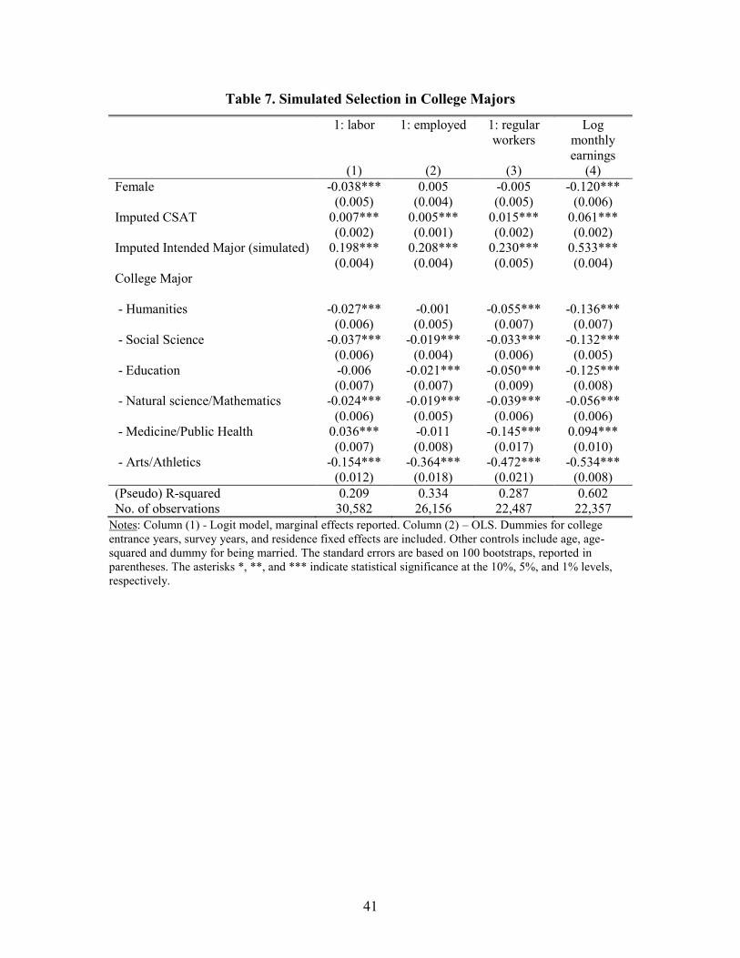
41

Table 7. Simulated Selection in College Majors

1: labor 1: employed 1: regular

workers

Log

monthly

earnings

(1) (2) (3) (4)

Female -0.038*** 0.005 -0.005 -0.120***

(0.005) (0.004) (0.005) (0.006)

Imputed CSAT 0.007*** 0.005*** 0.015*** 0.061***

(0.002) (0.001) (0.002) (0.002)

Imputed Intended Major (simulated) 0.198*** 0.208*** 0.230*** 0.533***

(0.004) (0.004) (0.005) (0.004)

College Major

- Humanities -0.027*** -0.001 -0.055*** -0.136***

(0.006) (0.005) (0.007) (0.007)

- Social Science -0.037*** -0.019*** -0.033*** -0.132***

(0.006) (0.004) (0.006) (0.005)

- Education -0.006 -0.021*** -0.050*** -0.125***

(0.007) (0.007) (0.009) (0.008)

- Natural science/Mathematics -0.024*** -0.019*** -0.039*** -0.056***

(0.006) (0.005) (0.006) (0.006)

- Medicine/Public Health 0.036*** -0.011 -0.145*** 0.094***

(0.007) (0.008) (0.017) (0.010)

- Arts/Athletics -0.154*** -0.364*** -0.472*** -0.534***

(0.012) (0.018) (0.021) (0.008)

(Pseudo) R-squared 0.209 0.334 0.287 0.602

No. of observations 30,582 26,156 22,487 22,357

Notes: Column (1) - Logit model, marginal effects reported. Column (2) – OLS. Dummies for college

entrance years, survey years, and residence fixed effects are included. Other controls include age, age-

squared and dummy for being married. The standard errors are based on 100 bootstraps, reported in

parentheses. The asterisks *, **, and *** indicate statistical significance at the 10%, 5%, and 1% levels,

respectively.

42

Table 8. College Majors and Labor Market Outcomes: Gender-Specific Returns

Outcome 1: labor 1: employed 1: regular

workers

Log monthly

earnings

Sample All Labor force

participants

Employees Employees

(1) (2) (3) (4)

College major

- Humanities -0.062*** -0.020** -0.098*** -0.217***

(0.013) (0.010) (0.016) (0.013)

- Social Science -0.031*** -0.002 -0.005 -0.034***

(0.008) (0.007) (0.009) (0.009)

- Education -0.037** -0.010 -0.127*** -0.159***

(0.016) (0.013) (0.022) (0.017)

- Natural science/Mathematics -0.063*** -0.052*** -0.074*** -0.108***

(0.011) (0.009) (0.013) (0.011)

- Medicine/Public Health 0.050*** -0.021 -0.231*** 0.086***

(0.015) (0.015) (0.027) (0.019)

- Arts/Athletics -0.031** -0.064*** -0.139*** -0.236***

(0.014) (0.013) (0.020) (0.015)

Female×College major

- ×Humanities 0.009 0.005 0.014 0.019

(0.014) (0.014) (0.014) (0.019)

- ×Social Science 0.018 -0.011 -0.012 -0.091***

(0.012) (0.014) (0.015) (0.016)

- ×Education 0.061*** 0.005 0.079*** 0.069***

(0.012) (0.016) (0.008) (0.022)

- ×Natural science/Mathematics 0.015 0.005 0.013 -0.036*

(0.012) (0.013) (0.013) (0.019)

- ×Medicine/Public Health 0.027 0.044*** 0.066*** 0.020

(0.024) (0.014) (0.009) (0.028)

- ×Arts/Athletics -0.005 -0.037** 0.027** -0.127***

(0.017) (0.018) (0.013) (0.022)

(Pseudo) R-squared 0.027 0.086 0.061 0.218

No. of observations 30,582 26,156 22,487 22,357

Notes: Columns (1) to (3) - Logit model, marginal effects reported. Column (4) - OLS. Dummies for

college entrance years, survey years, and residence fixed effects are included. Other controls include age,

age-squared and dummy for being married. The standard errors are in parentheses. The asterisks *, **, and

*** indicate statistical significance at the 10%, 5%, and 1% levels, respectively.