dhi glossary fact sheet - dairy records management systems
TRANSCRIPT
1
Aggregate eco-efficiency indices for New Zealand
– a Principal Components Analysis
Nigel Jollands
New Zealand Centre for Ecological Economics, Massey University and Landcare
Research, Palmerston North, New Zealand e-mail address: [email protected]
Jonathan Lermit
Consultant, Wellington New Zealand
Murray Patterson
New Zealand Centre for Ecological Economics, Massey University and Landcare
Research, Palmerston North, New Zealand
Paper presented at the 2004 NZARES Conference
Blenheim Country Hotel, Blenheim, New Zealand. June 25-26, 2004.
Copyright by author(s). Readers may make copies of this document for non-commercial
purposes only, provided that this copyright notice appears on all such copies.
2
Aggregate eco-efficiency indices for New Zealand – a
Principal Components Analysis
Nigel Jollandsa*
, Jonathan Lermitb and Murray Patterson
a
aNew Zealand Centre for Ecological Economics, Massey University and Landcare Research, Palmerston
North, New Zealand b Consultant, Wellington New Zealand
*Corresponding author:
Present Address: PO Box 11-052, Palmerston North, New Zealand
Tel +64 6 356 7154; fax +64 6 355 9230
Email address: [email protected]
“Everything should be as simple as possible, but not simpler”(Einstein in Meadows 1998, p. 22)
Abstract
Eco-efficiency has emerged as a management response to waste issues associated with current
production processes. Despite the popularity of the term in both business and government
circles, limited attention has been paid to measuring and reporting eco-efficiency to government
policy makers. Aggregate measures of eco-efficiency are needed, to complement existing
measures and to help highlight important patterns in eco-efficiency data.
This paper aims to develop aggregate measures of eco-efficiency for use by policy makers.
Specifically, this paper provides a unique analysis by applying principal components analysis
(PCA) to eco-efficiency indicators in New Zealand.
This study reveals that New Zealand's overall eco-efficiency improved for two out of the five
aggregate measures over the period 1994/95 to 1997/98. The worsening of the other aggregate
measures reflects, among other things, the relatively poor performance of the primary
production and related processing sectors. These results show PCA is an effective approach for
aggregating eco-efficiency indicators and assisting decision makers by reducing redundancy in
an eco-efficiency indicators matrix.
Keywords: Policy development; policy evaluation; Aggregate indices
Introduction
Eco-efficiency is a management response aimed at “curing” the “disease of wastefulness”
associated with current production processes (Weizsäcker et al. 1997). The concept of eco-
efficiency first entered academic literature in an article by Schaltegger and Sturm in 1990

3
(Schaltegger & Burritt 2000). However, Schmidheiny (1992) popularised the term, and
subsequently the concept of eco-efficiency has gained in popularity and spread throughout the
business world. Not surprisingly, eco-efficiency has received significant attention in the
sustainable-development literature, including this journal (Brady et al. 1999; Business Council
for Sustainable Development 1993; Choucri 1995; Cramer 1997; DeSimone et al. 2000; Metti
1999; Reith & Guirdy 2003; Schaltegger & Synnestvedt 2002; Weizsäcker et al. 1997)
Many authors have attempted to define eco-efficiency. For example, Williams (1999, p.37)
defines eco-efficiency as „endeavouring to get more from less for longer”. Metti (1999, p83)
states “eco-efficiency is simply creating more value with fewer materials and less water. One
definition of eco-efficiency that is gaining increasing currency comes from the World Business
Council for Sustainable Development (WBCSD):
“Eco-efficiency is reached by the delivery of competitively-priced goods and services that
satisfy human needs and bring quality life, which progressively reducing environmental impacts
and resource intensity throughout the life cycle, to a level at least in line with the earth’s
estimated carrying capacity” (DeSimone et al., 2000, p47).
Despite the range of interpretations, Hinterberger and Stiller (1998, p.275) note that all
definitions have an obvious theme in common; “All concepts call for a more efficient use of
natural resources.” Beyond that clearly, the detail of eco-efficiency can be understood in a
number of ways.
Schaltegger and Burritt (2000) suggest a distinction can be made between eco-efficiency as a
concept and as a ratio figure, although the two are linked. The eco-efficiency concept is a
relatively new derivation of „efficiency‟. Efficiency itself embodies the notion of “fitness or
power to accomplish, or success in accomplishing, the purpose intended” (Simpson & Weiner
1989 / p. 84). Adding the „eco-„ prefix to efficiency makes the eco-efficiency concept distinct
from the other efficiency concepts. The „eco-„ prefix focuses on the „environment and relation
to it.‟ (Barnhart 1998). Specifically, the prefix adds a lens to the „success in accomplishing‟
components of the efficiency concept. Through this lens, „success‟ is seen to extend beyond
4
simply whether the goal is achieved or not, to encompass a concern for the impact on „ the
environment and relation to it‟ associated with the activity of achieving the goal. The WBCSD,
for example promote the concept of eco-efficiency.
Often, in modern use of the term, eco-efficiency is measured using a ratio of useful outputs to
inputs. This ratio derives from 19th
Century thermodynamics and its empirical work on thermal
efficiency measures (Jollands 2003).
When applied to eco-efficiency, the ratio measures useful outputs (products, services etc) to
environmental inputs (Schaltegger & Burritt 2000). This ratio (or derivatives thereof) has been
employed in many eco-efficiency studies including Glauser & Muller (1997), Metti (1999) and
Schaltegger and Burritt (2000). In this study, we also operationalise the eco-efficiency concept
by way of a ratio.
A review of the eco-efficiency literature reveals several notable methodological gaps. One gap
that is the focus of this paper is the limited attention paid to measuring and reporting eco-
efficiency for government policy makers. A notable exception is the work being done in
Germany by the Wuppertal Institute (Bringezu 2004) and the German Federal Statistics office
(Hoh et al. 2001). This gap is all the more surprising, given the recent interest in eco-efficiency
by many government policy agencies and intergovernmental organisations (Organisation for
Economic Co-operation and Development 1998).
It is often argued that policy makers have specific requirements of indicators. Boisevert et al.
(1998, p.106-107) summarise policy makers' requirements into two broad needs:
Only a limited number of indicators should be used to convey the general state of the
environment. Too many indicators can compromise the legibility of the information.
Information should be presented in a format tailored to decision making. This requires
the construction of indicators that reduce the number of parameters needed to give a
precise account of a situation.

5
As a result of these specific requirements, many authors (for example Alfsen & Saebo 1993;
Heycox 1999; Luxem & Bryld 1997; Opschoor 2000) argue that aggregate indices that meet the
needs of decision makers are needed. Unfortunately, few researchers have heeded this call,
particularly in relation to eco-efficiency.
This paper attempts to provide aggregate indicators for policy makers. Specifically, it aims to
develop aggregate measures of eco-efficiency for use in national environmental policy. In
doing so, the paper briefly canvases the issues surrounding aggregate indices in general. It then
applies one aggregating method that has shown promise in other applications, principal
components analysis (PCA), to New Zealand data to reveal trends in eco-efficiency between
1994/95 and 1997/98.
Aggregate indices - brickbats and bouquets
The relative strengths and weaknesses of aggregate indices are well documented (see for
example Jollands, 2003). The main arguments can be summarised as follows.
Proponents of aggregate indices argue that indices assist decision makers by:
reducing the clutter of too much information (Alfsen & Saebo 1993; Callens & Tyteca
1999; Heycox 1999).
helping to communicate information succinctly and making patterns in the data easier to
see (Cleveland et al. 2000).
formalising the aggregation process that is often done implicitly.
Critics of aggregate indices offer equally persuasive arguments. They point out that
aggregate indices rely on potentially distorting assumptions (Lindsey et al. 1997).
it is difficult for aggregate indices to capture the necessary interrelationships within
complex environment-economy systems (Gustavson et al. 1999).
6
aggregation is often faced with the problem of adding together quantities measured in
different units. This is particularly the case with the economy-environment interface. In
this context Martinez-Alier et. al. (1998) argue that it is inappropriate to shoehorn such
disparate values into one cardinal set.
The two contesting views regarding aggregate indices are not as starkly opposed as may first
appear and are necessarily complementary. A high level of indicator aggregation is needed to
intensify the awareness of economy-environment interaction problems. But, even given the
advantages of aggregate indices, no single index can possibly answer all questions.
On balance, the most appropriate approach appears to be to use a judicious mix of detailed and
aggregated indices, and to treat aggregate indices with particular care.
Approaches to developing aggregate indices
Given that aggregate indices do have a role to play, how can aggregate eco-efficiency indices be
developed for New Zealand? Previous work by Jollands (2003) proposed a framework for
developing aggregate indices. One of the most challenging and contentious steps in developing
aggregate eco-efficiency indices is the setting of weightings needed for commensurating the
various aspects of eco-efficiency (such as water use and energy use) that are measured in
different units. Possible weighting schemes range from direct monetization, public opinion polls
and cost of distance to target, to ecological pricing and statistical methods (Jesinghaus 1997).
Considerable debate exists about which weighting scheme to use. This paper investigates the
use of a multi-variate statistical weighting approach, principal components analysis (PCA). PCA
has received little attention in aggregate indicator literature in general and eco-efficiency
literature specifically (with the notable exception of the work by Yu et al. (1998)).
The use of PCA offers several advantages. First, PCA is a useful alternative to the more
“subjective” weighting systems like public opinion polls. PCA weights data by combining
original variables into linear combinations that explain as much variation as possible. In this

7
way, PCA provides a relatively “objective” approach to setting weights that is dictated by the
data rather than the analyst. In effect, it “lets the data speak”.
Second, PCA is a useful tool for improving the “efficiency” of indicators (Callens & Tyteca
1999). A unique advantage of PCA is that it reports the amount of variance in the data that is
explained by the resulting aggregate indices.
Finally, PCA is designed to reduce the dimensionality of data sets. However, PCA is not a
panacea (Vega et al. 1998). In particular, PCA is limited to ex post analysis. It is not an
appropriate tool for prospective investigations. Nevertheless, given the strengths of PCA, it
would appear that the use of PCA could provide fertile ground for an inquiry into developing
aggregate measures of eco-efficiency.
Method –a brief description of PCA
Principal components analysis reduces a number of variables to a few indices (called the
principal components) that are linear combinations of the original variables (Heycox 1999
p.211; Manly 1994 p.12; Sharma 1996; Yu et al. 1998). PCA provides an objective way of
„aggregating‟ indicators so that variation in the data can be accounted for as concisely as
possible.
PCA takes p variables ε1, ε 2, ..., ε p and finds linear combinations of these to produce principal
components Z1, Z2, ...Zp (Manly 1994 p.78). Principal components are established by linear
transformations of the observed variables (ε i) under two conditions (Marcoulides &
Hershberger 1997). The first condition is that the first principal component accounts for the
maximum amount of variance possible, the second component that greatest amount of
remaining variance, and so on. The second condition is that all final components are
uncorrelated with each another. This lack of correlation is useful because it means that the
indices are measuring different „dimensions‟ in the data.
8
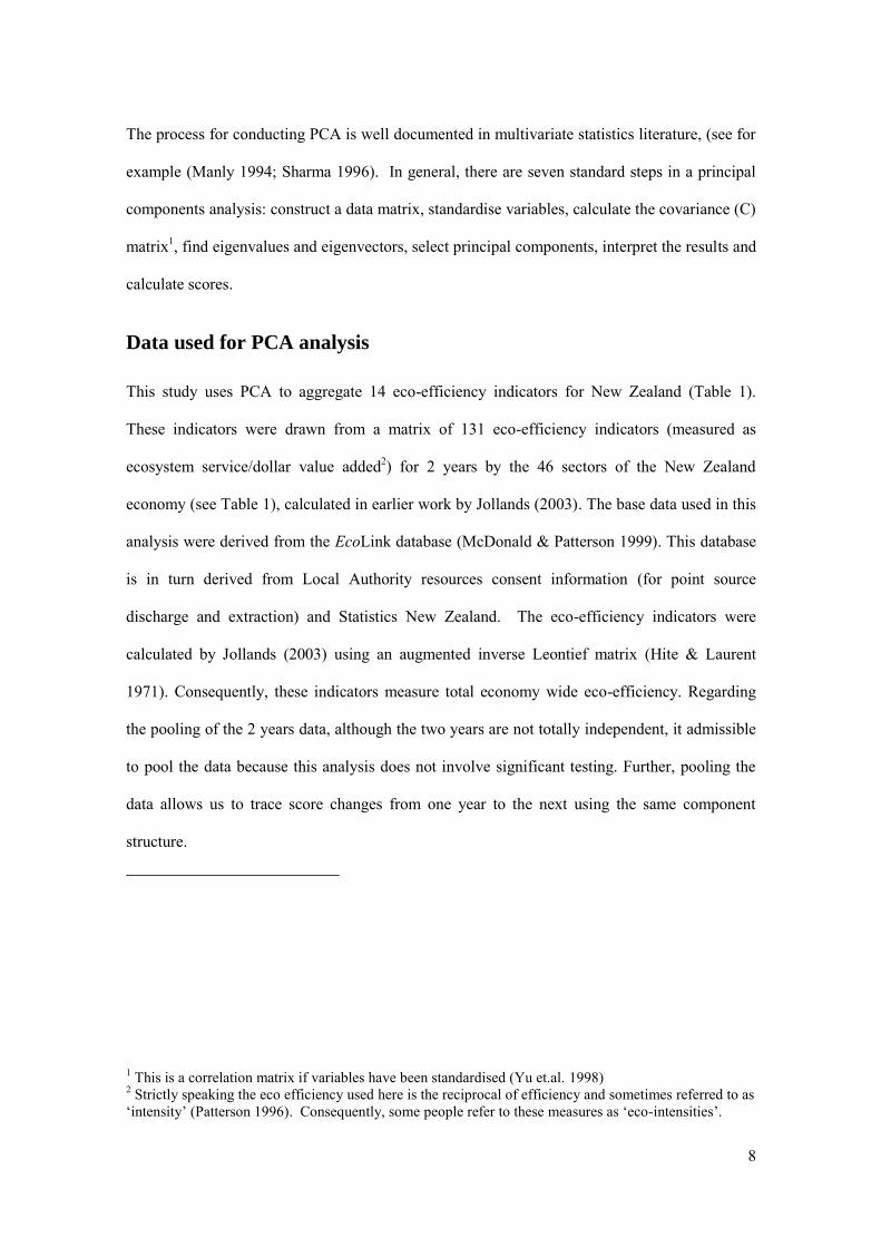
The process for conducting PCA is well documented in multivariate statistics literature, (see for
example (Manly 1994; Sharma 1996). In general, there are seven standard steps in a principal
components analysis: construct a data matrix, standardise variables, calculate the covariance (C)
matrix1, find eigenvalues and eigenvectors, select principal components, interpret the results and
calculate scores.
Data used for PCA analysis
This study uses PCA to aggregate 14 eco-efficiency indicators for New Zealand (Table 1).
These indicators were drawn from a matrix of 131 eco-efficiency indicators (measured as
ecosystem service/dollar value added2) for 2 years by the 46 sectors of the New Zealand
economy (see Table 1), calculated in earlier work by Jollands (2003). The base data used in this
analysis were derived from the EcoLink database (McDonald & Patterson 1999). This database
is in turn derived from Local Authority resources consent information (for point source
discharge and extraction) and Statistics New Zealand. The eco-efficiency indicators were
calculated by Jollands (2003) using an augmented inverse Leontief matrix (Hite & Laurent
1971). Consequently, these indicators measure total economy wide eco-efficiency. Regarding
the pooling of the 2 years data, although the two years are not totally independent, it admissible
to pool the data because this analysis does not involve significant testing. Further, pooling the
data allows us to trace score changes from one year to the next using the same component
structure.
1 This is a correlation matrix if variables have been standardised (Yu et.al. 1998)
2 Strictly speaking the eco efficiency used here is the reciprocal of efficiency and sometimes referred to as
„intensity‟ (Patterson 1996). Consequently, some people refer to these measures as „eco-intensities‟.

9
Table 1: List of sectors of the New Zealand economy used in this analysis
Sector number Sector name NZSIC codes
1 Mixed livestock 11120, 11130, 11140
2 Dairy farming 11110
3 Horticulture 11150, 11170, 11190
4 Services to Agriculture 112000
5 All other farming 11160
6 Fishing and Hunting 13000
7 Forestry & Logging 12000
8 Oil and Gas Exploration 22000
9 Other mining 29000, 23000, 21000
10 Meat Products 31110
11 Dairy Products 311120
12 Manufacture of other food 31100, 31200, 31100
13 Beverage Manufacture 31300, 31400
14 Textile Manufacture 32000
15 Wood & Wood Products 33000
16 Paper products 34100
17 Printing & Publishing 34200, 83402
18 Other Chemicals 35200, 35500, 35600
19 Basic Chemicals 35100, 35300, 35400
20 Non-metallic Minerals 36000
21 Basic Metal Industries 37000
22 Fabricated Metals 38100
23 Equipment Manufacture 38200-38500
24 Transport Equipment 38400
25 Other Manufacturing 39000
28 Water works 41030, 42000
29 Construction 53000
30 Trade 61000-62000
31 Accommodation 63000
32 Road transport 71120-71150
33 Services to Transport 71160-71190
34 Water Transport 71200
35 Air Transport 71300
36 Communications 72000
37 Finance 81100-81200
38 Finance services 81491-82300 excl 81200
39 Insurance 81200
40 Real Estate 83100
41 Business Services 83200
42 Dwelling ownership 83122
43 Education 93100-93200
44 Community Services 93300-93400
45 Recreation Services 93900-94900
46 Personal Services 95000, 93500, 92030, 92011, 92012, 92020
47 Central Government 91010
48 Local Government 91020
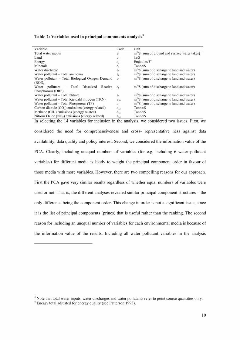
The 14 indicators chosen for inclusion in the analysis are shown in table 2.
10
Table 2: Variables used in principal components analysis3
Variable Code Unit
Total water inputs ε1 m3/$ (sum of ground and surface water takes)
Land ε2 ha/$
Energy ε3 Emjoules/$4
Minerals ε4 Tonne/$
Water discharge ε5 m3/$ (sum of discharge to land and water)
Water pollutant – Total ammonia ε6 m3/$ (sum of discharge to land and water)
Water pollutant – Total Biological Oxygen Demand
(BOD5)
ε7 m3/$ (sum of discharge to land and water)
Water pollutant – Total Dissolved Reative
Phosphorous (DRP)
ε8 m3/$ (sum of discharge to land and water)
Water pollutant – Total Nitrate ε9 m3/$ (sum of discharge to land and water)
Water pollutant – Total Kjeldahl nitrogen (TKN) ε10 m3/$ (sum of discharge to land and water)
Water pollutant – Total Phosporous (TP) ε11 m3/$ (sum of discharge to land and water)
Carbon dioxide (CO2) emissions (energy related) ε12 Tonne/$
Methane (CH4) emissions (energy related) ε13 Tonne/$
Nitrous Oxide (NO2) emissions (energy related) ε14 Tonne/$
In selecting the 14 variables for inclusion in the analysis, we considered two issues. First, we
considered the need for comprehensiveness and cross- representative ness against data
availability, data quality and policy interest. Second, we considered the information value of the
PCA. Clearly, including unequal numbers of variables (for e.g. including 6 water pollutant
variables) for different media is likely to weight the principal component order in favour of
those media with more variables. However, there are two compelling reasons for our approach.
First the PCA gave very similar results regardless of whether equal numbers of variables were
used or not. That is, the different analyses revealed similar principal component structures – the
only difference being the component order. This change in order is not a significant issue, since
it is the list of principal components (princs) that is useful rather than the ranking. The second
reason for including an unequal number of variables for each environmental media is because of
the information value of the results. Including all water pollutant variables in the analysis
3 Note that total water inputs, water discharges and water pollutants refer to point source quantities only.
4 Energy total adjusted for energy quality (see Patterson 1993).

11
revealed an interesting relationship that would have been overlooked had arbitrarily a single
„representative‟ water quality variable been arbitrarily selected (see the discussion of „prin 4‟
below).
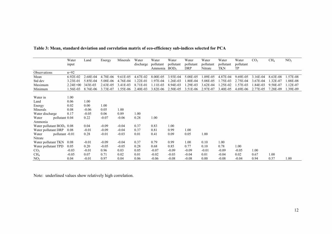
For each of the 14 variables, there were 92 observations (46 sectors by 2 years), which greatly
exceeds the 3 to 1 ratio regarded as the minimum requirement in PCA to provide a stable
solution (Grossman et al. 1991; Yu et al. 1998). Table 3 gives the mean value, standard
deviation maximum and minimum for each of the 14 variables. The covariance matrix of the 14
variables was calculated from standardised data and, therefore, coincides with the correlation
matrix (also shown in Table 3). Some clear eco-efficiency relationships can readily be inferred:
for example there were high positive correlations (underlined values) between water discharges
and minerals (r=0.89); the various water pollutants (r= 0.68 to 1.0); and energy and air
emissions (r = 0.71 to 0.97).
12
Table 3: Mean, standard deviation and correlation matrix of eco-efficiency sub-indices selected for PCA
Water
input
Land Energy Minerals Water
discharge
Water
pollutant
Ammonia
Water
pollutant
BOD5
Water
pollutant
DRP
Water
pollutant
Nitrate
Water
pollutant
TKN
Water
pollutant
TP
CO2 CH4 NO2
Observations n=92
Mean 6.92E-02 2.68E-04 4.78E-06 9.61E-05 4.67E-02 8.00E-05 3.93E-04 5.08E-05 1.09E-05 4.87E-04 9.69E-05 3.16E-04 8.63E-08 1.57E-08
Std dev 3.23E-01 5.85E-04 5.08E-06 4.76E-04 1.22E-01 1.97E-04 1.26E-03 1.80E-04 5.08E-05 1.75E-03 2.75E-04 3.67E-04 1.32E-07 1.88E-08
Maximum 2.24E+00 343E-03 2.63E-05 3.41E-03 8.71E-01 1.11E-03 8.94E-03 1.29E-03 3.62E-04 1.25E-02 1.57E-03 1.84E-03 9.58E-07 1.12E-07
Minimum 1.56E-03 8.76E-06 3.73E-07 1.55E-06 2.40E-03 3.82E-06 2.50E-05 3.51E-06 2.97E-07 3.40E-05 4.69E-06 2.77E-05 7.28E-09 1.39E-09
Water in
1.00
Land 0.06 1.00
Energy 0.02 0.00 1.00
Minerals 0.08 -0.06 0.05 1.00
Water discharge 0.17 -0.05 0.06 0.89 1.00
Water pollutant
Ammonia
0.04 0.22 -0.07 -0.06 0.28 1.00
Water pollutant BOD5 0.08 0.04 -0.09 -0.04 0.37 0.83 1.00
Water pollutant DRP 0.08 -0.01 -0.09 -0.04 0.37 0.81 0.99 1.00
Water pollutant
Nitrate
-0.01 0.28 -0.01 -0.03 0.01 0.41 0.09 0.05 1.00
Water pollutant TKN 0.08 -0.01 -0.09 -0.04 0.37 0.79 0.99 1.00 0.10 1.00
Water pollutant TPD 0.05 0.20 -0.05 -0.05 0.28 0.68 0.85 0.77 0.10 0.78 1.00
CO2 -0.03 -0.01 0.96 0.03 0.05 -0.07 -0.09 -0.09 -0.01 -0.09 -0.05 1.00
CH4 -0.05 0.07 0.71 0.02 0.01 -0.02 -0.03 -0.04 0.01 -0.04 0.02 0.67 1.00
NO2 0.04 -0.01 0.97 0.04 0.06 -0.06 -0.08 -0.08 0.00 -0.08 -0.04 0.94 0.57 1.00
Note: underlined values show relatively high correlation.

13
Results and Discussion
The PCA was performed using the PRINCOMP procedure of the SAS system (SAS Institute
1985), which standardises data to zero mean and unit variance. This standardisation is
important in this study, given that the variables display widely different means and relatively
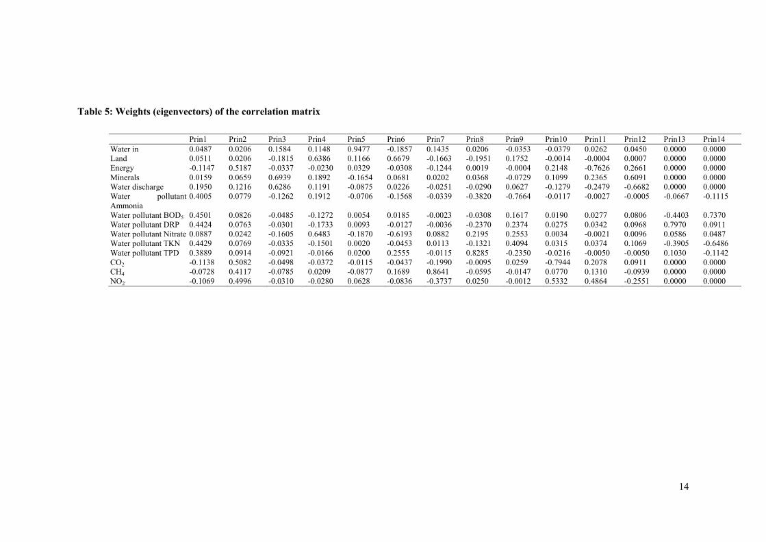
large standard deviations (see Table 2). The eigenvalues and eigenvectors of the correlation
matrix are given in Tables 4 and 5, respectively.
Table 4: Eigenvalues of the correlation matrix
Eigenvalue Difference Proportion Cumulative
1 4.6720 1.2777 0.3337 0.3337
2 3.3943 1.5273 0.2425 0.5762
3 1.8670 0.5356 0.1334 0.7095
4 1.3314 0.3441 0.0951 0.8046
5 0.9872 0.2249 0.0705 0.8751
6 0.7623 0.2846 0.0545 0.9296
7 0.4777 0.2005 0.0341 0.9637
8 0.2772 0.1291 0.0198 0.9835
9 0.1481 0.0927 0.0106 0.9941
10 0.0554 0.0386 0.0040 0.9980
11 0.0169 0.0063 0.0012 0.9992
12 0.0106 0.0106 0.0008 1.0000
13 0.0000 0.0000 0.0000 1.0000
14 0.0000 0.0000 0.0000 1.0000
14
Table 5: Weights (eigenvectors) of the correlation matrix
Prin1 Prin2 Prin3 Prin4 Prin5 Prin6 Prin7 Prin8 Prin9 Prin10 Prin11 Prin12 Prin13 Prin14
Water in 0.0487 0.0206 0.1584 0.1148 0.9477 -0.1857 0.1435 0.0206 -0.0353 -0.0379 0.0262 0.0450 0.0000 0.0000
Land 0.0511 0.0206 -0.1815 0.6386 0.1166 0.6679 -0.1663 -0.1951 0.1752 -0.0014 -0.0004 0.0007 0.0000 0.0000
Energy -0.1147 0.5187 -0.0337 -0.0230 0.0329 -0.0308 -0.1244 0.0019 -0.0004 0.2148 -0.7626 0.2661 0.0000 0.0000
Minerals 0.0159 0.0659 0.6939 0.1892 -0.1654 0.0681 0.0202 0.0368 -0.0729 0.1099 0.2365 0.6091 0.0000 0.0000
Water discharge 0.1950 0.1216 0.6286 0.1191 -0.0875 0.0226 -0.0251 -0.0290 0.0627 -0.1279 -0.2479 -0.6682 0.0000 0.0000
Water pollutant
Ammonia
0.4005 0.0779 -0.1262 0.1912 -0.0706 -0.1568 -0.0339 -0.3820 -0.7664 -0.0117 -0.0027 -0.0005 -0.0667 -0.1115
Water pollutant BOD5 0.4501 0.0826 -0.0485 -0.1272 0.0054 0.0185 -0.0023 -0.0308 0.1617 0.0190 0.0277 0.0806 -0.4403 0.7370
Water pollutant DRP 0.4424 0.0763 -0.0301 -0.1733 0.0093 -0.0127 -0.0036 -0.2370 0.2374 0.0275 0.0342 0.0968 0.7970 0.0911
Water pollutant Nitrate 0.0887 0.0242 -0.1605 0.6483 -0.1870 -0.6193 0.0882 0.2195 0.2553 0.0034 -0.0021 0.0096 0.0586 0.0487
Water pollutant TKN 0.4429 0.0769 -0.0335 -0.1501 0.0020 -0.0453 0.0113 -0.1321 0.4094 0.0315 0.0374 0.1069 -0.3905 -0.6486
Water pollutant TPD 0.3889 0.0914 -0.0921 -0.0166 0.0200 0.2555 -0.0115 0.8285 -0.2350 -0.0216 -0.0050 -0.0050 0.1030 -0.1142
CO2 -0.1138 0.5082 -0.0498 -0.0372 -0.0115 -0.0437 -0.1990 -0.0095 0.0259 -0.7944 0.2078 0.0911 0.0000 0.0000
CH4 -0.0728 0.4117 -0.0785 0.0209 -0.0877 0.1689 0.8641 -0.0595 -0.0147 0.0770 0.1310 -0.0939 0.0000 0.0000
NO2 -0.1069 0.4996 -0.0310 -0.0280 0.0628 -0.0836 -0.3737 0.0250 -0.0012 0.5332 0.4864 -0.2551 0.0000 0.0000


16
Five principal components retained
Several tests are available for determining how many principal components (PCs) to retain.
Cattel‟s Scree plot of eigenvalues, the Jollife-amended Kaiser eigenvalue criterion and an
examination of the proportion of variance accounted for by the principal components suggests
retaining five PCs (which account for around 87% of the variation) (Table 3). Note that the
order in which the principal components are listed in Table 3 reflects the order in which they are
derived from the PCA. It does not necessarily reflect their relative importance in characterising
eco-efficiency.
The five principal components
The first principal component (Prin1) accounts for 33.4% of the total variation in the data (Table
3). Algebraically, Prin1 is shown as:
Prin1 =0.048ε1+0.051ε2–0.115ε3+0.016ε4+0.195ε5+0.400ε6+
0.450ε7+0.442ε8+0.088ε9+0.443ε10+0.389ε11–0.114ε12–
0.073ε13–0.107ε14
Equation 1
Where ε1 to ε14 are the original eco-efficiency indicators used in the analysis.
Table 5 and the equation above show that Prin1 has high positive coefficients (weights) on
ammonia water pollution (0.400), biological oxygen demand (BOD5) (0.405), dissolved reactive

17
phosphorous (DRP) (0.442), total kjeldahl nitrogen (TKN) (0.443) and total phosphorous (TP)
(0.389); i.e., on all water pollutant indicators except nitrates5. Prin1 can be called water-
pollutant intensity, with higher Prin1 scores indicating higher water pollutant intensity (m3/$).
The prominence of water pollutants in this analysis is interesting, since the issue of greatest
concern to New Zealanders is the pollution of New Zealand‟s freshwater resources (Ministry for
the Environment 2001).
The second principal component, Prin2, accounts for a further 24% of the total variation in the
data, and has high positive weights on energy (0.519) and air emission indicators (0.508, 0.412,
0.499 for CO2, CH4 and NO2 respectively). Prin2 can be interpreted as energy and energy-
related air emission intensity, with higher scores indicating higher energy and energy-related air
emission intensities.
Prin3 accounts for a further 13% of the total variation. Compared to the first two principal
components, the interpretation of Prin3 is less intuitive. It has large positive coefficients on
mineral-input (0.694) and water-discharge (0.629) intensities. Other mining is a significant
source of point-source water discharge in New Zealand. The dominance of the other mining
(which includes iron sand mining) sector‟s water discharge intensity helps to explain the
prominence of water discharge in Prin3. Given that mineral inputs „drive‟ this principal
component, this component could be interpreted as „material intensity,‟ with higher scores
indicating greater mineral-input and water discharge intensities. Interestingly the negative
5 This appears to be because point source nitrate levels are closely linked to the meat products sector,
which has a significant level of „embodied‟ land. Therefore, the PCA analysis traces land and nitrate
pollutants in a separate principal component.

18
coefficients on 11 of the 14 variables are likely to have a dampening effect on this component‟s
scores.
The fourth principal component, Prin4, accounts for a further 9.5% of the total variation. Prin4
is highly participated by land intensity (0.639) and water pollutant (nitrate) (0.648). This is an
interesting result, and one that could have been overlooked, had not all water pollutant variables
been included in the analysis. The link between land and nitrate intensities is expected, and an
analysis of the meat products sector helps to explain this link. The meat products sector is a
significant source of point-source discharge of nitrates and accounts for approximately 96% of
measured point-source nitrate discharges. Furthermore, this sector‟s total land intensity (ha/$) is
second only to that of mixed livestock. That is, meat product outputs contain significant
„embodied‟ land. Given that the nitrates measured in this analysis derive from land, Prin4 can
be interpreted to represent land intensities, with higher scores meaning higher land intensities.
The fifth principal component, Prin5, accounts for 7% of the total variation. Prin5 is dominated
by water inputs6, making interpretation of this component straightforward. Prin5 can be
interpreted as water-input intensity, with higher scores meaning higher water-input intensities.
These five principal components are useful for decision makers. Not only do they summarise
92 x 14 points of data, but also they represent the most important dimensions of eco-efficiency
from an explained variance point of view, given the available data (the components explain
almost 90% of the variation in all 14 variables). The five principal components also meet a
priori expectations, in that they summarise the important energy and material flows through the
6 To both water „suppliers‟ and water „consumers‟ (see below).
19
economy that are covered in the analysis. Note, however, that data constraints mean that many
environmental media are not covered in this analysis (for example, non-point source emissions).
A fruitful area of future research would be to expand the PCA to cover a broader data set.
Aggregate scores for New Zealand
Individual sector scores for each principal component can be calculated by solving the principal
component equations (such as Equation 1). The sector scores can be used to calculate overall
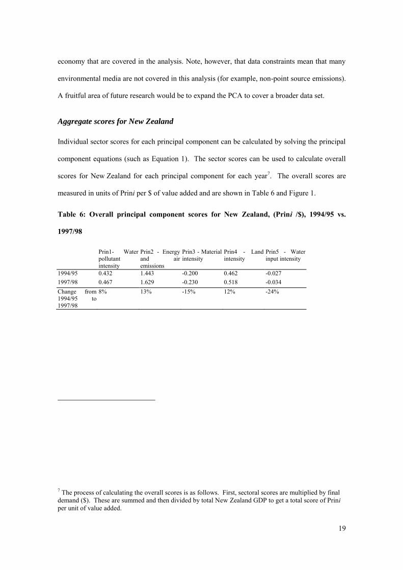
scores for New Zealand for each principal component for each year7. The overall scores are
measured in units of Prini per $ of value added and are shown in Table 6 and Figure 1.
Table 6: Overall principal component scores for New Zealand, (Prini /$), 1994/95 vs.
1997/98
Prin1- Water
pollutant
intensity
Prin2 - Energy
and air
emissions
Prin3 - Material
intensity
Prin4 - Land
intensity
Prin5 - Water
input intensity
1994/95 0.432 1.443 -0.200 0.462 -0.027
1997/98 0.467 1.629 -0.230 0.518 -0.034
Change from
1994/95 to
1997/98
8% 13% -15% 12% -24%
7 The process of calculating the overall scores is as follows. First, sectoral scores are multiplied by final
demand ($). These are summed and then divided by total New Zealand GDP to get a total score of Prini
per unit of value added.
20
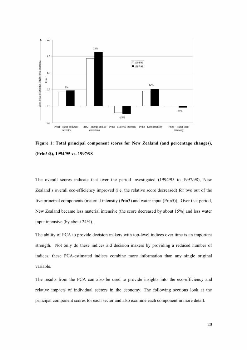
Figure 1: Total principal component scores for New Zealand (and percentage changes),
(Prini /$), 1994/95 vs. 1997/98
The overall scores indicate that over the period investigated (1994/95 to 1997/98), New
Zealand‟s overall eco-efficiency improved (i.e. the relative score decreased) for two out of the
five principal components (material intensity (Prin3) and water input (Prin5)). Over that period,
New Zealand became less material intensive (the score decreased by about 15%) and less water
input intensive (by about 24%).
The ability of PCA to provide decision makers with top-level indices over time is an important
strength. Not only do these indices aid decision makers by providing a reduced number of
indices, these PCA-estimated indices combine more information than any single original
variable.
The results from the PCA can also be used to provide insights into the eco-efficiency and
relative impacts of individual sectors in the economy. The following sections look at the
principal component scores for each sector and also examine each component in more detail.
-0.5
0.0
0.5
1.0
1.5
2.0
Prin1- Water pollutant
intensity
Prin2 - Energy and air
emissions
Prin3 - Material intensity Prin4 - Land intensity Prin5 - Water input
intensity
1994/95
1997/98
Wors
e e
co-e
ffic
iency (
hig
her
eco-i
nte
nsi
ty)
Pri
ni/ $
8%
13%
-15%
12%
-24%
21
Sector eco-efficiency scores
Sectors showing poor eco-efficiency in multiple dimensions
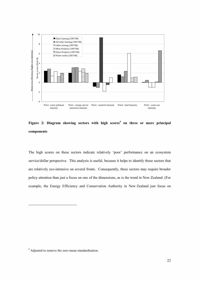
PCA can help identify those sectors demonstrating poor eco-efficiency across most or all of the
five important dimensions. For example, one sector has relatively high scores8 across all five
principal components (water works). This result appears counter intuitive since one would not
expect the water works sector to have high material intensity. However, prin 3 (material
intensity) also has a high coefficient on water discharge (volume). Since this sector processes
and filters water for most other sectors, it is reasonable to expect a high score for this sector on
water discharge (and therefore a high Prin 3 score). One sector has high scores on four principal
components (other mining, which has high scores on all components except water input
(Prin5)). In addition, four sectors show high scores on three principal components (Prin1, 2 and
4) simultaneously (other farming, dairy farming, meat products and dairy products). The
component scores for these sectors are shown in Figure 2.
8 Defined in this instance as being „greater than one.‟
22
Figure 2: Diagram showing sectors with high scores9 on three or more principal
components
The high scores on these sectors indicate relatively „poor‟ performance on an ecosystem
service/dollar perspective. This analysis is useful, because it helps to identify those sectors that
are relatively eco-intensive on several fronts. Consequently, these sectors may require broader
policy attention than just a focus on one of the dimensions, as is the trend in New Zealand. (For
example, the Energy Efficiency and Conservation Authority in New Zealand just focus on
9 Adjusted to remove the zero-mean standardisation.
-4
-2
0
2
4
6
8
10
Prin1- water pollutant
intensity
Prin2 - energy and air
emissions intensity
Prin3 - material intensity Prin4 - land intensity Prin5 - water use
intensity
Dairy farming (1997/98)
All other farming (1997/98)
Other mining (1997/98)
Meat Products (1997/98)
Dairy Products (1997/98)
Water works (1997/98)
Wors
e e
co-e
ffic
iency (
hig
her
eco-i
nte
nsi
ty)
Secto
r sc
ore
s (P
rini
/$)

23
energy efficiency, whereas for the sectors mentioned in this section, the focus needs to be
broadened to overall eco-efficiency.)
Further insights into New Zealand‟s eco-efficiency are possible from an analysis of each
principal component in turn.
Prin1 – water-pollutant intensity
Prin1 by definition explains the greatest amount of variation in the eco-efficiency indicator data
of all the principal components. It is interesting to note that the pollution of New Zealand‟s
freshwater resources is an issue of concern to New Zealanders (Ministry for the Environment
2001), giving this principal component added interest.
The overall score for Prin1 increased slightly (by 8%) over the analysis period, suggesting that
New Zealand as a whole is increasing the amount of water pollution discharged per dollar of
output (see Table 6 and Figure 1). This result is consistent with findings in New Zealand‟s State
of the Environment report (Ministry for the Environment, 1997) that documents the increasing
pressure on New Zealand‟s water ways over this period.
The personal services sector has the highest score on Prin110
. This sector is plotted against
other relatively high Prin1 sector scores for 1997/98 in Figure 3.
The Prin1 scores for the personal services sector declined by 8% between 1994/95 to 1997/98,
probably as a result of standard management practice to continually improve plant efficiency
through capital replacement.
10 The reason for this is the inclusion in the personal services sector of the „sewerage and urban drainage‟
(NZSIC 92012) sector.
24
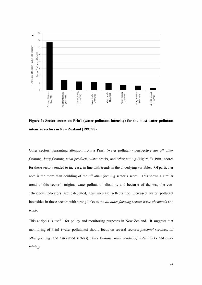
Figure 3: Sector scores on Prin1 (water pollutant intensity) for the most water-pollutant
intensive sectors in New Zealand (1997/98)
Other sectors warranting attention from a Prin1 (water pollutant) perspective are all other
farming, dairy farming, meat products, water works, and other mining (Figure 3). Prin1 scores
for these sectors tended to increase, in line with trends in the underlying variables. Of particular
note is the more than doubling of the all other farming sector‟s score. This shows a similar
trend to this sector‟s original water-pollutant indicators, and because of the way the eco-
efficiency indicators are calculated, this increase reflects the increased water pollutant
intensities in those sectors with strong links to the all other farming sector: basic chemicals and
trade.
This analysis is useful for policy and monitoring purposes in New Zealand. It suggests that
monitoring of Prin1 (water pollutants) should focus on several sectors: personal services, all
other farming (and associated sectors), dairy farming, meat products, water works and other
mining.
0
2
4
6
8
10
12
14
16
Pers
onal
Serv
ices
(1997/9
8)
All
oth
er
farm
ing
(1997/9
8)
Dair
y f
arm
ing
(1997/9
8)
Meat
Pro
ducts
(1997/9
8)
Wate
r w
ork
s
(1997/9
8)
Oth
er
min
ing
(1997/9
8)
Dair
y P
roducts
(1997/9
8)
Mix
ed l
ivest
ock
(1997/9
8)
Secto
r P
rin1 s
core
(P
rin1/$
)
Wors
e e
co-e
ffic
iency (
hig
her
eco-i
nte
nsi
ty)
25
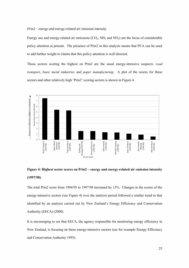
Prin2 – energy and energy-related air emission intensity
Energy use and energy-related air emissions (CO2, NH4 and NO2) are the focus of considerable
policy attention at present. The presence of Prin2 in this analysis means that PCA can be used
to add further weight to claims that this policy attention is well directed.
Those sectors scoring the highest on Prin2 are the usual energy-intensive suspects: road
transport, basic metal industries and paper manufacturing. A plot of the scores for these
sectors and other relatively high „Prin2‟ scoring sectors is shown in Figure 4.
Figure 4: Highest sector scores on Prin2 – energy and energy-related air emission intensity
(1997/98)
The total Prin2 score from 1994/95 to 1997/98 increased by 13%. Changes in the scores of the
energy-intensive sectors (see Figure 4) over the analysis period followed a similar trend to that
identified by an analysis carried out by New Zealand‟s Energy Efficiency and Conservation
Authority (EECA) (2000).
It is encouraging to see that EECA, the agency responsible for monitoring energy efficiency in
New Zealand, is focusing on these energy-intensive sectors (see for example Energy Efficiency
and Conservation Authority 1995).
0
1
2
3
4
5
6
7
8
Ro
ad
Tra
nsp
ort
(19
97
/98
)
Bas
ic M
eta
l
Ind
ust
ries
(19
97
/98
)
Pap
er p
rod
uct
s
(19
97
/98
)
Fis
hin
g a
nd
Hu
nti
ng
(1
99
7/9
8)
Pers
on
al S
erv
ices
(19
97
/98
)
Oth
er m
inin
g
(19
97
/98
)
All
oth
er f
arm
ing
(19
97
/98
)
Dai
ry P
rod
uct
s
(19
97
/98
)
No
n-m
etal
lic
Min
eral
s
(19
97
/98
)
Mea
t P
rod
ucts
(19
97
/98
)
Sect
or
Pri
n2
Sco
re (
Pri
n2
/$)
Sector (year)
Wors
e e
co-e
ffic
iency (
hig
her
eco-i
nte
nsi
ty)

26
Prin3 – material intensity
This PCA has helped to highlight the important role of mineral inputs in the New Zealand
economy. Specifically, there are important links between the other mining sector and non-
metallic minerals and basic metal industries.
The other mining, waterworks11
and non-metallic minerals sectors had the highest Prin3 scores.
A plot of the score for these sectors and other relatively high Prin3 scoring sectors is shown in
Figure 5.
Figure 5: Highest sector scores on Prin3 – material intensity (1997/98)
Changes in these sectors‟ scores between 1994/95 and 1997/98 confirm findings in other
analyses (Jollands 2003). Prin3 is highly participated by water discharged indicators, so it is not
11 Because of the high water discharge component of this sector.
0
1
2
3
4
5
6
7
8
9
10
Oth
er m
inin
g
(19
97
/98
)
Wat
er w
ork
s
(19
97
/98
)
No
n-m
etal
lic
Min
eral
s
(19
97
/98
)
Bas
ic C
hem
icals
(19
97
/98
)
Oth
er
Man
ufa
ctu
rin
g
(19
97
/98
)
Oil
an
d G
as
Ex
plo
rati
on
(19
97
/98
)
Bas
ic M
eta
l
Ind
ust
ries
(19
97
/98
)
Sect
or
Pri
n3
Sco
re (
Pri
n3
/$)
Sector (year)
Wors
e e
co-e
ffic
iency (
hig
her
eco-i
nte
nsi
ty)

27
surprising to find that waterworks scores relatively highly on Prin3. The waterworks sector
showed a decline in its Prin3 score (of around 20%). This follows a trend in the underlying
indicators: water-discharge indicators declined by around 42 percent over the period.
Prin4 – land intensity
Land input is essential for all economic sectors. Furthermore, Prin4 is highly participated by
nitrate pollutant. Nitrate pollution in waterways is of concern because nitrate is a significant
source of eutrophication (McDonald & Patterson 1999).
The sectors with the three highest Prin4 scores are the meat products, mixed livestock and other
mining sectors.
These sectors had increased Prin4 scores over the period, except meat products. The Prin4
score for the meat products sector decreased by 6%. This decrease follows a decrease in nitrate
indicator of 4% and an increase in land intensity of 4%. The Prin4 score for the mixed livestock
sector increased over the period, suggesting that this sector is becoming more land and nitrate-
pollutant intensive. Data produced by Statistics New Zealand confirms that land intensity has
increased for the mixed livestock sector (Statistics New Zealand 2004).
A useful feature of this PCA is its ability to highlight sectors warranting policy intervention. An
analysis of sector scores suggests the two sectors warranting policy and monitoring attention are
the mixed livestock and meat products sectors. These sectors are the most land and nitrate
intensive, and the meat products sector in particular contributes a significant proportion of
point-source nitrate pollutants.
Prin5 – water input intensity
This component is dominated by water inputs. Water is an essential ecosystem good and is
required as an input (directly and indirectly) in all economics sectors. The highest scores on
Prin5 were for the other mining and meat products sectors.
28
The high water input intensity of the other mining sector is primarily due to the titanomagnetite
mining operation at Waikato Heads. Water is used to assist the transport of about 82kt of ore per
week via an 18km pipeline to a steel mill. The meat products sector also has one of the highest
water input intensities. Water is used in this sector primarily in cleaning and rendering. Scores
on these sectors show that the other mining sector‟s Prin5 score increased (by 16%) while its
water-input intensity increased by 18%. In contrast, the meat products sector‟s Prin5 score
decreased.
Conclusion
Eco-efficiency has emerged as a management response to waste issues associated with current
production processes. Eco-efficiency can be understood in terms of concept, or a ratio of useful
output to environmental inputs. Despite the popularity of the term in both business and
government circles, limited attention has been paid to measuring and reporting eco-efficiency to
government policy makers. In particular, there is a need for aggregate measures of eco-
efficiency to complement existing measures and help to highlight important patterns in eco-
efficiency data.
This study investigated eco-efficiency through principal components analysis (PCA), a
statistical technique that has shown promise but has had little attention for analysing eco-
efficiency indicators. Conducting PCA on an eco-efficiency indicator matrix of two-years data
over the 46 sectors in New Zealand revealed several strengths of the technique. First, PCA
identified five important dimensions of the eco-efficiency data from an explained variance point
of view: water pollutant, energy and energy-related air emissions, materials, land, and water
input intensities. In doing so, PCA is able to reduce redundancy in the eco-efficiency indicator
profile while providing results that are consistent with the findings of the more detailed matrix.
29
Second, PCA can provide the much sought-after „aggregate‟ scores for each dimension
(principal component). These scores supply condensed information for decision makers and
provide an overall assessment of New Zealand‟s eco-efficiency trends.
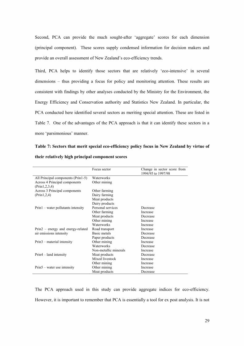
Third, PCA helps to identify those sectors that are relatively „eco-intensive‟ in several
dimensions – thus providing a focus for policy and monitoring attention. These results are
consistent with findings by other analyses conducted by the Ministry for the Environment, the
Energy Efficiency and Conservation authority and Statistics New Zealand. In particular, the
PCA conducted here identified several sectors as meriting special attention. These are listed in
Table 7. One of the advantages of the PCA approach is that it can identify these sectors in a
more „parsimonious‟ manner.
Table 7: Sectors that merit special eco-efficiency policy focus in New Zealand by virtue of
their relatively high principal component scores
Focus sector Change in sector score from
1994/95 to 1997/98
All Principal components (Prin1-5) Waterworks
Across 4 Principal components
(Prin1,2,3,4)
Other mining
Across 3 Principal components
(Prin1,2,4)
Other farming
Dairy farming
Meat products
Dairy products
Prin1 – water pollutants intensity Personal services
Other farming
Meat products
Other mining
Waterworks
Decrease
Increase
Decrease
Increase
Increase
Prin2 – energy and energy-related
air emissions intensity
Road transport
Basic metals
Paper products
Increase
Decrease
Decrease
Prin3 – material intensity Other mining
Waterworks
Non-metallic minerals
Increase
Decrease
Increase
Prin4 – land intensity Meat products
Mixed livestock
Other mining
Decrease
Increase
Increase
Prin5 – water use intensity Other mining
Meat products
Increase
Decrease
The PCA approach used in this study can provide aggregate indices for eco-efficiency.
However, it is important to remember that PCA is essentially a tool for ex post analysis. It is not
30
an appropriate tool for ex ante analysis. Nevertheless, this type of analysis warrants further
investigation as a legitimate aggregation approach.
In conclusion, it is useful to draw on the pertinent message from Costanza (2000, p.342). “Even
given [the] advantage of aggregate indicators, no single one can possibly answer all questions
and multiple indicators will always be needed … as will intelligent and informed use of the ones
we have”. This conclusion goes without saying. Thus, aggregate indices provide a necessary
but not completely sufficient, contribution to the debate of eco-efficiency issues, as well as the
policy responses to those issues.
References
Alfsen K. H. & Saebo H. V. (1993) Environmental quality indicators: background, principles
and examples from Norway. Environmental and Resource Economics 3: 415-435.
Boisevert V., Holec N. & Vivien D. (1998) Economic and Environmental Information for
Sustainability. In: Valuation for sustainable development: methods and policy indicators (eds.
S. Faucheux & M. O'Connor) pp. 99-119. Edward Elgar Publishing Ltd, Cheltenham.
Brady K., Henson P. & Fava J. (1999) Sustainability, Eco-efficiency, life cycle management
and business strategy. In: Environmental Quality Management pp. 33-41.
Bringezu S. (2004) Measuring Eco-Efficiency on the Basis of Input and Output oriented
indicators. In: 2004 Eco-Efficiency Conference - Quantified methods for decision making,
Leiden, The Netherlands.
Business Council for Sustainable Development (1993) Getting Eco-Efficient, Report of the
Business Council for Sustainable Development, First Antwerp Eco-Efficiency Workshop.
Business Council for Sustainable Development, Geneva.
Callens I. & Tyteca D. (1999) Towards indicators of sustainable development for firms.
Ecological Economics 28: 41-53.
Choucri N. (1995) Globalisation of eco-efficiency: GSSD on the WWW. In: UNEP Industry
and Environment.
Cleveland C. J., Kaufmann R. K. & Stern D. I. (2000) Aggregation and the role of energy in the
economy. Ecological Economics 32: 301-317.
Costanza R. (2000) The dynamics of the ecological footprint concept. Ecological Economics 32:
341-345.
Cramer J. (1997) How can we substantially increase eco-efficiency? UNEP Industry and
Environment July - September: 58-62.
DeSimone L. D., Popoff F. & Development W. B. C. f. S. (2000) Eco-efficiency: The Business
Link to Sustainable Development. The MIT Press.
Energy Efficiency and Conservation Authority (1995) Energy-Wise Monitoring Quarterly, Issue
2. Energy Efficiency and Conservation Authority, Wellington.
Energy Efficiency and Conservation Authority (2000) The dynamics of energy efficiency trends
in New Zealand: a compendium of energy end-use analysis and statistics. Energy Efficiency and
Conservation Authority, Wellington.
Glauser M. & Muller P. (1997) Eco-effiency: a prerequisite for future success. CHIMIA 51:
201-206.
31
Grossman G., Nickerson D. & Freeman M. (1991) Principal Component Analyses of
Assemblage Structured Data: Utility of tests based on eigenvalues. Ecology 72: 341-347.
Gustavson K., Longeran S. & Ruitenbeek H. J. (1999) Selection and modelling of sustainable
development indicators: a case study of the Fraser River Basin, British Columbia. Ecological
Economics 28: 117-132.
Heycox J. (1999) Integrating data for sustainable development: introducing the distribution of
resources framework. In: Novartis Foundation Symposium 220: Environmental statistics -
analysing data for environmental policy pp. 191-212. John Wiley & Sons, London.
Hite J. & Laurent E. A. (1971) Empirical Study of Economic-Ecologic Linkages in a Coastal
Area. Water Resources Research 7: 1070-1078.
Hoh H., Scoer K. & Seibel S. (2001) Eco-Efficiency Indicators in German Environmental-
Economic Accounting. Federal Statistical Office, Germany.
Jesinghaus J. (1997) Current approaches to valuation. In: Sustainability Indicators: a Report on
the Project on Indicators of Sustainable Development (eds. B. Moldan, S. Billharz & R.
Matravers) pp. 84-91. John Wiley & Sons on behalf of the Scientific Committee on Problems of
the Environment (SCOPE), New York.
Jollands N. (2003) An Ecological Economics of Eco-Efficiency: Theory, Interpretations and
Applications to New Zealand. Massey University, PhD Thesis.
Lindsey G., Wittman J. & Rummel M. (1997) Using indices in Environmental Planning:
evaluating policies for wellfield protection. Journal of Environmental Planning and
Management 40: 685-703.
Luxem M. & Bryld B. (1997) Introductory Box: the CSD Work Programme on Indicators of
Sustainable Development. In: Sustainability Indicators: a Report on the Project on Indicators of
Sustainable Development (eds. B. Moldan, S. Billharz & R. Matravers) pp. 6-12. John Wiley &
Sons on behalf of the Scientific Committee on Problems of the Environment (SCOPE), New
York.
Manly B. (1994) Multivariate statistical methods: a primer. Chapman & Hall, London.
Marcoulides G. A. & Hershberger S. (1997) Multivariate statistical methods - a first course.
Lawrence Erlbaum Associates, Mahwah, New Jersey.
Martinez-Alier J., Munda G. & O'Neill J. (1998) Weak comparability of values as a foundation
for ecological economics. Ecological Economics 26: 277-286.
McDonald G. & Patterson M. G. (1999) EcoLink Economic Accounts - Technical Report.
Massey University and McDermot Fairgray, Palmerston North.
Meadows D. (1998) Indicators and information for sustainable development. The Sustainability
Institute, USA.
Metti G. (1999) Global Environmental factors and eco-efficiency. In: Beverage World pp. 82-
83.
Ministry for the Environment (2001) Your views about our environment.
Opschoor H. (2000) Ecological footprint: measuring rod or metaphor? Ecological Economics
32: 363-365.
Organisation for Economic Co-operation and Development (1998) Eco-efficiency. OECD, Paris.
Patterson M. G. (1993) Approaches to Energy Quality in Energy Analysis. International
Journal of Global Energy Issues, Special Issue on Energy analysis 5: 19-28.
Patterson M. G. (1996) What is energy efficiency? Concepts, issues and methodological issues.
Energy Policy 24: 377-390.
Reith C. & Guirdy M. (2003) Eco-efficiency analysis of an agricultural research complex.
Journal of Environmental Management 68: 219-229.
SAS Institute (1985) User's Guide: Statistics. SAS Institute Inc., Cary, USA.
Schaltegger S. & Burritt R. (2000) Contemporary Environmental Accounting - issues, concepts
and practice. Greenleaf Publishing, Sheffield.
Schaltegger S. & Synnestvedt T. (2002) The link between 'green' and economic success:
environmental management as the crucial trigger between environmental and economic
performance. Journal of Environmental Management 65: 339-346.
32
Schmidheiny S. (1992) Changing Course. MIT Press, Cambridge, Massachusetts.
Sharma S. (1996) Applied Multivariate Techniques. John Wiley & Sons, New York.
Simpson J. & Weiner E. (1989) The Oxford English Dictionary. Clarendon Press, Oxford.
Statistics New Zealand (2004) Animal farming in New Zealand.
Vega M., Pardo R., Barrado E. & Debán L. (1998) Assessmentof seasonal and polluting effects
on the quality of river water by exploratory data analysis. Water Research 32: 3581-3592.
Weizsäcker v. E. U., Lovins A. & Lovins H. (1997) Factor four: doubling wealth - halving
resource use. Earthscan, London.
Yu C., Quinn J. T., Dufournaud C. M., Harrington J. J., Rogers P. P. & Lohani B. N. (1998)
Effective dimensionality of environmental indicators: a principal component analysis with
bootstrap confidence intervals. Journal of Environmental Management 53: 101-119.