development of novel computational...
TRANSCRIPT

Sede amministrativa: Universita degli studi di Padova
Dipartimento di Ingegneria dell’Informazione
SCUOLA DI DOTTORATO DI RICERCA IN: Ingegneria dell’Informazione
INDIRIZZO: Bioingegneria
CICLO XXIV
DEVELOPMENT OF NOVEL COMPUTATIONAL
ALGORITHMS FOR QUANTITATIVE
VOXEL-WISE FUNCTIONAL BRAIN IMAGING
WITH POSITRON EMISSION TOMOGRAPHY
Direttore della scuola: Ch.mo Prof. Matteo Bertocco
Supervisore: Prof. Alessandra Bertoldo
Dottorando: Gaia Rizzo

Contents
Summary v
Sommario ix
1 Introduction 1
2 PET receptor kinetic models 9
2.1 Two tissue-four rate constants plasma input model . . . . . . . . . 10
2.2 Two tissue-three rate constants plasma input model . . . . . . . . 12
2.3 One tissue-two rate constants plasma input model . . . . . . . . . 14
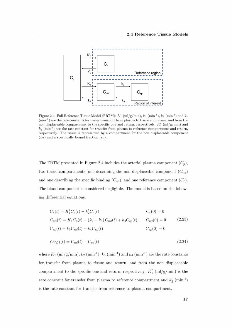
2.4 Reference Tissue Models . . . . . . . . . . . . . . . . . . . . . . . . 16
2.4.1 Full Reference Tissue Model . . . . . . . . . . . . . . . . . . 16
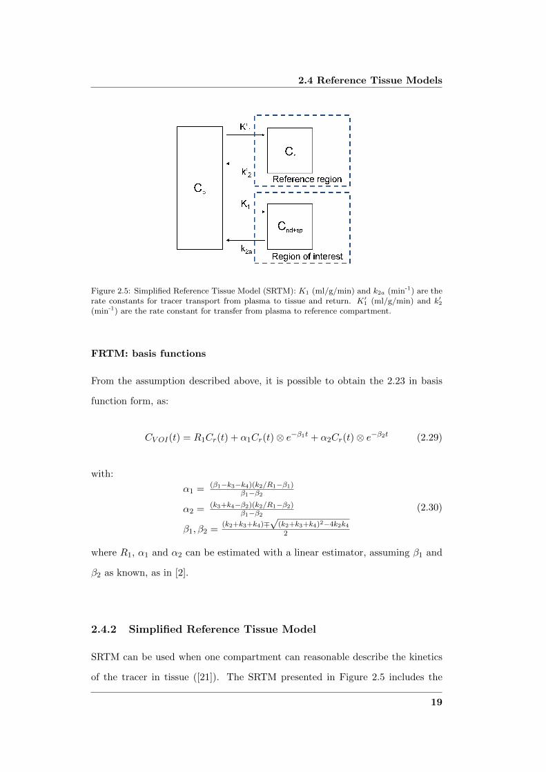
2.4.2 Simplified Reference Tissue Model . . . . . . . . . . . . . . 19
3 Novel approaches for Bayesian voxel-wise PET quantification 23
3.1 Bayesian PET modeling . . . . . . . . . . . . . . . . . . . . . . . . 23
3.2 Hierarchical Maximum a Posteriori (H-MAP) . . . . . . . . . . . . 28
3.3 Hierarchical Basis Function Method (H-BFM) . . . . . . . . . . . . 29
4 Image Acquisition and Processing 33
4.1 Datasets and Processing . . . . . . . . . . . . . . . . . . . . . . . . 33
4.1.1 [11C]DPN (Opioid receptor ligand) . . . . . . . . . . . . . . 33
4.1.2 [11C]FLB457 (Dopamine receptor ligand) . . . . . . . . . . 35
i
CONTENTS
4.1.3 [11C]WAY100635 (Serotonin receptor ligand) . . . . . . . . 38
4.1.4 [11C]SCH442416 (Adenosine receptor ligand) . . . . . . . . 39
4.1.5 [11C]MDL100907 (Serotonin receptor ligand) . . . . . . . . 41
4.2 Automatic generation of ROIs: atlas vs cluster . . . . . . . . . . . 44
5 Application on datasets 47
5.1 H-MAP on [11C]DPN . . . . . . . . . . . . . . . . . . . . . . . . . 47
5.2 H-BFM on [11C]WAY100635 and [11C]FLB457 . . . . . . . . . . . 53
6 Results 59
6.1 H-MAP results . . . . . . . . . . . . . . . . . . . . . . . . . . . . . 59
6.1.1 Discussion . . . . . . . . . . . . . . . . . . . . . . . . . . . . 66
6.2 H-BFM results . . . . . . . . . . . . . . . . . . . . . . . . . . . . . 68
6.2.1 Discussion . . . . . . . . . . . . . . . . . . . . . . . . . . . . 74
6.3 Results based on functional clustering . . . . . . . . . . . . . . . . 75
7 Additional work: development of novel compartmental models
for quantification of PET tracer kinetics 79
7.1 Modeling [11C]SCH442416 dataset . . . . . . . . . . . . . . . . . . 80
7.1.1 Model structure . . . . . . . . . . . . . . . . . . . . . . . . 81
7.1.2 4K-2IF model results . . . . . . . . . . . . . . . . . . . . . . 84
7.1.3 3K-parallel model results . . . . . . . . . . . . . . . . . . . 87
7.1.4 Discussion . . . . . . . . . . . . . . . . . . . . . . . . . . . . 90
7.2 Modeling [11C]MDL100907 dataset . . . . . . . . . . . . . . . . . . 92
7.2.1 Metabolite curve fitting . . . . . . . . . . . . . . . . . . . . 93
7.2.2 Classic Spectral Analysis (SA) . . . . . . . . . . . . . . . . 94
7.2.3 Non Linear Spectral Analysis (NLSA) . . . . . . . . . . . . 96
7.2.4 NLSA results: ROI analysis . . . . . . . . . . . . . . . . . . 98
7.2.5 SA results: voxel analysis . . . . . . . . . . . . . . . . . . . 100
7.2.6 Discussion . . . . . . . . . . . . . . . . . . . . . . . . . . . . 103
ii
CONTENTS
7.2.7 Method for the selection of the optimal reference region . . 109
8 Overall discussion 113
8.1 Compartmental modeling at voxel level . . . . . . . . . . . . . . . 113
8.2 Comparison of the novel methods with existing methodologies . . . 114
8.2.1 Global Two Stage . . . . . . . . . . . . . . . . . . . . . . . 117
8.2.2 Iterative Two Stage . . . . . . . . . . . . . . . . . . . . . . 119
8.3 Development of an alternative clustering algorithm . . . . . . . . . 121
8.4 Conclusions . . . . . . . . . . . . . . . . . . . . . . . . . . . . . . . 123
Bibliography 124
iii

Summary
Positron Emission Tomography (PET) allows to study, in vivo, important bio-
logical processes in both animals and humans. In particular, it is widely used for
receptor studies, where it allows quantitative functional imaging of physiological
parameters in terms of receptor binding, volume of distribution, and/or receptor
occupancy.
The radioactivity concentration measured with PET can be related to the un-
derlying physiological processes using appropriate tracer kinetic modeling tech-
niques, generally compartmental models. Once the best compartmental structure
describing the behavior of the tracer has been defined, it is possible to estimate
the system’s micro or macro parameters. This can be achieved at the Region of
Interest (ROI) level, i.e. generating a tissue Time Activity Curve (TAC) of the
average activity concentration within a specific brain area, or at the voxel level,
i.e. deriving the tissue TAC from one single image unit.
The ROI level approach is commonly used to quantify PET images by using
nonlinear estimators since ROI TACs are characterized by a good signal-to-noise
ratio. However, the use of ROI TACs causes a loss of spatial resolution since it
does not allow the quantification of the physiological information with the same
spatial detail as the acquired PET data.
Voxel level analysis allows avoiding operator-dependency of manually delineated
ROIs and produces parametric maps having the same spatial resolution as the
v

Summary
original PET image. However, TACs derived from a voxel are characterized by
a low signal-to-noise ratio. This renders the use of nonlinear estimators difficult
and unwieldy because of their computational cost. Thus, more robust and faster
estimation algorithms are necessary in order to quantify the physiological infor-
mation at the voxel level within reasonable computational time.
The purpose of this work is to propose and develop methods to quantify PET
tracer activity at voxel level, overcoming the limitations of the approaches al-
ready present in literature.
In Chapter 1 an overview on the basis of kinetic modeling in PET and a report
of the state of the art literature of the topic will be given. Diverse approaches
are available for quantification at the voxel level, such as generalized linear least
square ([1]), basis function methods (BFMs) ([2], [3], [4]), spectral analysis ([5]),
population methods as Global Two Stage (GTS, [6]), Bayesian estimation ([7]),
and graphical approaches such as the Patlak and Logan plots ([8], [9], [10]). Each
of them will be presented with their advantages and drawbacks.
In Chapter 2 an overview of the main PET receptor compartmental models is
presented, both models with plasma input function and models with reference
input function, which are of particular interest as they allow obviating the need
for invasive arterial plasma measurements during the PET exam.
In Chapter 3 the proposed novel approaches for Bayesian quantification will be
presented. In Section 3.1 the principles of Bayesian estimation are given. In
Section 3.2 a general approach to generate parametric maps that consists in a
multi-stage hierarchical method will be investigated. Kinetic information are
transmitted from the regions to the voxels using a maximum a posteriori (MAP)
estimator. A Bayesian estimator considers as known the a priori probability of
vi

the model parameters and updates the prior probability itself using the measured
data ([11]). When the prior distribution is derived from the data, the method is
referred as empirical Bayes.
In Section 3.3 a new hierarchical method to apply BFM to multicompartmen-
tal models is investigated. The grids for the basis functions are generated au-
tomatically from the data, specifically for each ROI, being consequently user-
indipendent. The local grids for the voxel-by-voxel analysis are defined a priori,
using the estimates obtained by application of the optimal model for the ROI
TACs and solving with a non linear estimator, the gold standard method.
In Chapter 4 the datasets available are presented. Six different datasets were
made available by Division of Experimental Medicine, Imperial College of London
(UK) and by the Institute San Raffaele of Milan (Italy). In particular, datasets
of [11C]DPN (selective antagonist at opioid receptors), [11C]FLB457 (high affin-
ity dopamine D2/D3 receptor radioligand), [carbonyl -11]WAY100635 (selective
serotonin 5-HT1A receptor antagonist), [11C]MDL100907 (high affinity serotonin
5-HT2A ligand) and [11C]SCH442416 (highly selective adenosine A2A antagonist)
were available. An alternative method for the ROI segmentation by using cluster
analysis is also presented in Section 4.2, in order to assess the effect on the results
of the different ways to extract the priors.
In Chapter 5 the application of the methods presented above on the various
datasets will be illustrated and in Chapter 6 the results obtained with the differ-
ent methods will be reported and discussed.
In Chapter 7 some additional aims of this work are presented, in particular the
development of compartmental model for quantification of PET tracer kinetics.
Both novel methods are model-driven methods, based on compartmental models.
Consequently, the primary aim of the work has been the identification of the
vii

Summary
optimal model to describe the data, in case it was not already presented in litera-
ture. A new compartmental model for [11C]SCH442416 and for [11C]MDL100907
dataset was developed. [11C]SCH442416 data have never been quantified with
compartmental models in humans before and for [11C]MDL100907 the model
presented in literature was not appropriate for the fit of the available data.
In Chapter 8 an overall discussion and conclusions are presented. In particular,
in Section 8.2 a comparison with existing methodologies is implemented, focusing
on population methods, as Global and Iterative Two Stage.
The main results of this work are the development of two methods for voxel-wise
quantification of PET data, H-MAP and H-BFM. The methods are a good al-
ternative for the generation of reliable parametric maps, and applied to clinical
data are expected to simplify r the detection also of small/specific pathological
areas. The first method led to a publication in Neuroimage ([12]), the second was
presented during two international conferences (BrainPET2011 and SNM2011)
as oral contribution and a publication is ready to be submitted.
The novel methods proposed have been already inserted in PIWAVE, a pre-
existing software for voxel-wise PET quantification originally developed by Im-
perial College of London.
As additional results, an alternative method for the ROI segmentation by using
cluster analysis was implemented and a new compartmental model for [11C]SCH-
442416 and [11C]MDL100907 data was developed. A new method for the selection
of the optimal reference region was implemented and applied on [11C]MDL100907
data.
viii
Sommario
La Tomografia ad Emissione di Positroni (PET) permette di studiare, in vivo,
l’interazione dei traccianti con specifici siti di legame (trasportatori, recettori,
etc.). Inoltre permette un imaging funzionale quantitativo di importanti parametri
fisiologici quali la densita di recettori, volume di distribuzione e/o occupazione
recettoriale.
La concentrazione di radioattivita misurata con la PET puo essere messa in re-
lazione con i processi fisiologici usando appropriate strategie modellistiche, in
genere modelli compartimentali. Una volta definita la struttura compartimen-
tale che meglio descrive le cinetiche del tracciante, e possibile stimare i micro o
macro parametri del sistema. Tale analisi puo essere eseguita a livello di regione
di interesse (ROI - Region of Interest), cioe generando una curva (TAC - Time
Activity Curve) della concentrazione di radioattivita media in una specifica area
cerebrale, o a livello di voxel, cioe derivando la curva tessutale da un singolo
elemento dell’immagine.
L’approccio a livello di regione e usato solitamente per quantificare immagini
PET con stimatori non lineari dato che le curve tessutali di regione sono carat-
terizzate da un buon rapporto segnale disturbo. Tuttavia, l’analisi a livello di
regione comporta una perdita in risoluzione spaziale, dato che non permette di
quantificare l’informazione fisiologica con lo stesso dettaglio spaziale delle immag-
ini acquisite.
ix
Sommario
L’analisi a livello di voxel permette di evitare la selezione a mano (dipendente
dall’operatore) delle regioni e produce mappe parametriche con la stessa risoluzione
spaziale dell’immagine PET originale. Tuttavia, le TAC derivate da un voxel sono
caratterizzate da un basso rapporto segnale disturbo e cio rende l’uso di stimatori
non lineari difficile e inefficiente, dato il loro costo computazionale. Sono quindi
necessari algoritmi di stima piu robusti e veloci per quantificare l’informazione
fisiologica a livello di voxel in un tempo ragionevole.
Obiettivo di questo lavoro e proporre e sviluppare metodi per la quantificazione di
immagini PET a livello di voxel, superando le limitazioni dei metodi gia presenti
in letteratura.
Nel Capitolo 1 e presentata una panoramica dei principali metodi modellistici in
PET e una rassegna sullo stato dell’arte. Vari approcci sono gia disponibili per
la quantificazione a livello di voxel, come il generalized linear least square ([1]),
basis function methods (BFMs) ([2], [3], [4]), spectral analysis ([5]), metodi di
popolazione come Global Two Stage (GTS, [6]), stima Bayesiana ([7]), e metodi
grafici quali il Patlak e Logan plots ([9], [10]). Per ognuno di questi verranno
descritti vantaggi e limiti.
Il Capitolo 2 espone una panoramica dei principali modelli compartimentali re-
cettoriali, sia modelli con ingresso la curva dell’attivita plasmatica del tracciante,
che modelli a regione di riferimento, di particolare interesse poiche permettono
di evitare l’invasivo campionamento arteriale durante l’esame PET.
Il Capitolo 3 propone i nuovi approcci Bayesiani sviluppati per la quantificazione
PET. Nella Sezione 3.1 sono presentati i principi di stima Bayesiana. Nella
Sezione 3.2 viene descritto un approccio generale per la generazione di mappe
parametriche, basato su un metodo gerarchico multi-livello. Le informazioni ci-
netiche ottenute per la regione vengono trasmesse ai voxel appartenenti a cias-
x

cuna classe con uno stimatore Maximum A Posteriori (MAP). Uno stimatore
Bayesiano considera nota la probabilita a priori dei parametri del modello e la
aggiorna basandosi sui dati misurati ([11]). Quando l’informazione a priori e
derivata dai dati, il metodo e detto Bayesiano empirico.
La Sezione 3.3 descrive un nuovo metodo gerarchico per applicare il metodo BFM
a modelli multi compartimentali. Le griglie per le funzioni base sono generate
automaticamente dai dati, specifiche per ogni regione, e di conseguenza in modo
indipendente dall’utente. Le griglie locali per l’analisi a livello di voxel sono defi-
nite a priori, usando le stime ottenute applicando il modello ottimo alle curve di
regione e risolvendolo con uno stimatore non lineare, che rappresenta il metodo
gold standard.
Nel Capitolo 4 sono presentati i sei dataset messi a disposizione dalla Division
of Experimental Medicine, Imperial College of London (UK) e dall’Istituto San
Raffaele di Milano (Italia). I dataset disponibili constano di dati di [11C]DPN
(antagonista selettivo ai recettori oppiodi), [11C]FLB457 (radioligando ad alta
affinita per i recettori di dopamina D2/D3), [carbonyl -11]WAY100635 (antago-
nista selettivo ai recettori di serotonina 5-HT1A), [11C]MDL100907 (ligando ad
alta affinita per i recettori di serotonina 5-HT2A) e [11C]SCH442416 (antago-
nista altamente selettivo ai recettori di adenosina A2A) Viene inoltre presentato
un metodo alternativo per la segmentazione delle ROI tramite cluster analysis
(Sezione 4.2), per valutare l’effetto dei diversi modi di estrarre i priors sui risultati.
Nel Capitolo 5 si presenta l’applicazione dei metodi descritti in precedenza sui
vari dataset e nel Capitolo 6 vengono descritti e discussi i risultati ottenuti.
Il Capitolo 7 espone alcuni obiettivi aggiuntivi di questo lavoro, in partico-
lare lo sviluppo di modelli compartimentali per la quantificazione delle cinetiche
di traccianti PET. I nuovi metodi proposti sono model-driven, basati cioe su
xi

Sommario
modelli compartimentali. Di conseguenza l’obiettivo iniziale del lavoro e stato
l’identificazione del miglior modello per descrivere i dati, qualora tale modello
non fosse gia presente in letteratura. Un nuovo modello compartimentale e stato
sviluppato per il dataset di dati [11C]SCH442416 e per i dati di [11C]MDL100907.
I dati di [11C]SCH442416 non sono mai stati analizzati in precedenza con modelli
compartimentali nell’uomo e per i dati da [11C]MDL100907 il modello presentato
in letteratura non e stato invece adatto a descrivere i dati a disposizione.
Nel Capitolo 8 si espongono la discussione complessiva e le conclusioni. In par-
ticolare, nella Sezione 8.2 si presenta un confronto dei metodi sviluppati con le
metodologie esistenti, con speciale attenzione ai metodi di popolazione, come il
Global e Iterative Two Stage.
I principali risultati di questo lavoro consistono nello sviluppo di due metodi per
la quantificazione di dati PET a livello di voxel, H-MAP e H-BFM. I metodi
costituiscono un’alternativa per la generazione di mappe parametriche affidabili
ed applicate a dati clinici renderanno piu semplice il riconoscimento di piccole
zone patologiche specifiche. Il primo metodo ha portato ad una pubblicazione su
Neuroimage ([12]), il secondo lavoro e stato presentato durante due conferenze
internazionali (BrainPET2011 e SNM2011) come oral presentation e una pubbli-
cazione e in fase di sottomissione.
Come ulteriore risultato, e stato implementato un metodo alternativo per la seg-
mentazione di regioni tramite cluster analysis ed e stato sviluppato un nuovo
modello compartimentale per i dati di [11C]SCH442416 e di [11C]MDL100907.
Inoltre e stato implementato un nuovo metodo per la selezione della migliore
regione di riferimento ed e stato applicato su immagini di [11C]MDL100907.
xii

Chapter 1
Introduction
Positron Emission Tomography (PET) is a functional nuclear medicine imaging
technique widely used to study in vivo physiological processes in the body. After
injection of a radiotracer (i.e. a positron-emitting radionuclide) into a patient,
a normal volunteer or a research animal, PET instrumentation detects pairs of
gamma rays generated after annihilation of any emitted positron with any elec-
tron of the surrounding material. Four-dimensional images representing the ra-
dioactivity concentration of the injected tracer over time are generated with an
appropriate reconstruction algorithm and with proper corrections for the physical
effects such as attenuation, dead time and scatter.
The radioactivity concentration measured during a dynamic PET exam can be
related to the underlying physiological processes using appropriate tracer kinetic
modeling techniques, where the model input is either the time course of the tracer
concentration in plasma or, for receptor studies, that of the tracer concentration
in an appropriate region, called reference region, devoid of receptors specific for
the tracer under examination. The kinetic analysis allows quantitative functional
imaging of physiological parameters such as blood flow, rate of glucose consump-
tion or amount of binding of the tracer to its specific receptors, depending upon
the tracer in use.
1
Introduction
These modeling techniques can be divided into model-driven methods and data-
driven methods. The distinction is that data-driven methods do not require any
a priori definition of the best model structure, but this information is derived
directly from the kinetic data. There are three data-driven methods developed
for quantitative PET analysis: graphical analysis (Patlak plot, [8], [9], and Logan
plot, [10]), spectral analysis ([5]) and basis pursuit ([13]).
Graphical methods are model-independent methods and allow fast estimation
of the parameters of interest through a transformation of the data that, after
a certain time t > t∗, shows a linear trend, whose slope can be related to the
parameter of interest. However it is possible to estimate only one macro system
parameter.
In spectral analysis ([5]) the kinetic activity of the tracer in the tissue is described
by the sum of decaying exponentials convolved with an input function, and the
coefficients of a predefined set of biologically plausible exponential basis functions
are estimated using nonnegative least squares to fit the data. Spectral analysis
also returns information on the number of compartments necessary to describe
the data.
Basis pursuit denoising ([13]) is an alternative approach to solve the linear system
of equations of spectral analysis, and includes a regularization term. Also this
technique returns parameter estimates that describe the transfer function of the
system, information on the number of components and on the type of kinetics.
Thus graphical methods allow the estimation of only macroparameters but they
are easy and fast to implement. Spectral analysis and basis pursuit allow to char-
acterize the transfer function of the system but the relation of these parameters to
measures of the physiological process of interest is possible only with knowledge
of the biochemical properties of the tracer and with the definition of the model
structure. In general data-driven methods allow generation of reliable parametric
maps and require less restrictive hypothesis compared to model-driven methods.
In order to apply model-driven methods it is instead necessary to define the com-
2

partmental structure that best describe the behavior of the tracer, with specific
assumptions on the number of compartments and their connections. It is thus
possible to relate the parameters to specific physiological measures. In PET, the
kinetic rate constants of the compartmental model are called micro parameters.
Well-established compartmental models in PET include those used for the quan-
tification of blood flow ([14]), cerebral metabolic rate for glucose ([15]), and for
neuroreceptor ligand binding ([16]).
Further developments have produced models using the reference tissue as model
input, thus avoiding the need for blood sampling ([17], [18], [19], [20], [21]). Micro
or macro system parameters are obtained using a least squares fitting procedure
such as linear least squares ([22]), non linear least squares ([22]), generalized lin-
ear least squares ([1]) or basis function techniques ([2]).
Among the various modeling techniques, compartmental modeling represents the
gold standard in PET quantification. The analysis can be applied both at the Re-
gion of Interest (ROI) level, i.e. generating a tissue Time Activity Curve (TAC)
of the average activity concentration within a specific brain area, or at the voxel
level, i.e. deriving the tissue TAC from one single image unit. In the ROI level
approach PET data are quantified using nonlinear estimators since ROI TACs
are characterized by a good signal-to-noise ratio. However, the use of ROI TACs
causes a loss of spatial resolution since it does not allow the quantification of the
physiological information with the same spatial detail as the acquired PET data.
Voxel level analysis allows avoiding operator-dependency of manually delineated
ROIs and produces parametric maps having the same spatial resolution as the
original PET image. However, TACs derived from a voxel are characterized by
a low signal-to-noise ratio. This renders the use of nonlinear estimators difficult
and unwieldy because of their computational cost. Thus, more robust and faster
estimation algorithms are necessary in order to quantify the physiological infor-
mation at the voxel level within reasonable computational time.
3

Introduction
Diverse approaches are available for quantification at the voxel level based on
compartmental modeling, such as generalized linear least square (GLLS) ([1]),
basis function methods (BFMs) ([2], [3] and [4]), Global Two Stage (GTS, [6])
and Bayesian estimation ([23], [7]).
In the GLLS approach, the model is linearized and then solved iteratively via
linear least square in order to eliminate the bias introduced by the linearization
of the model. The method was proven to lead to precise and accurate results
in the presence of low noise levels when the model which describes the data is
composed of two compartments, but its performance deteriorates rapidly at high
noise levels ([24]), typical of TACs derived from a single voxel. Moreover, the
choice of the termination criterion is crucial and GLLS’s computational cost can
be high or at least not negligible.
Among the so-called ”population approaches”, developed and largely used in
pharmacokinetic/pharmacodynamic studies, GTS is an iterative method which
has been demonstrated to be utilizable in quantitative PET for the generation of
parametric maps and tested on Simplified Reference Tissue Model (SRTM, [20])
and simulated 2-tissue PET data. In this approach, the estimates for each voxel
are iteratively updated using both the population variability and the precision of
the individual estimates. However, the performance of the method is sensitive to
the goodness of the initial values and to the noise level of PET data ([6]).
BFMs is the most used method, in which a grid consisting of exponential terms
convolved with the input function is defined a priori and the model is then solved
with linear estimators. It is commonly used as it can be easily applied to SRTM.
The method presents certain limitations, such as user-defined grids, fixed for all
subjects and brain voxels. Moreover, the choice of the grid can heavily penalize
the results and can lead to bias in the final estimates, which can also be affected
by the presence of noise in the data ([25]).
The BFMs have been also applied on multi-compartmental models, but the grids
were still fixed and very dense and the quantification was computationally de-
4

manding ([3]).
Among the Bayesian methods, in the linear and non linear ridge regression with
spatial constraints by Zhou et al. ([23], [26]) the parametric images obtained with
linear regression are spatially smoothed and then used as spatial constraints for
a second iteration of ridge regression. In particular, the a priori information is
provided for each voxel by the TACs of the voxels in its neighborhood, making
the method appropriate only for linear models, as the computational cost would
be too high for clinical routine use in case of non linear models.
The Bayesian method proposed by [7] is based on a nonlinear estimator and uses
prior information obtained by analyzing a prior cohort of parametric images. This
implies both the need of a high computational time and the necessity of having
an additional sufficiently large data set to derive reliable a priori information.
The purpose of this work was to propose and develop methods to quantify PET
tracer activity at voxel level, overcoming the limitations of the methods above,
e.g. the use of global and user-defined grids and the necessity of choosing a ter-
mination criterion, and to avoid the sensitivity to initial estimates.
At first a general approach to generate parametric maps that consists in a multi-
stage hierarchical method was investigated. Kinetic information obtained an-
alyzing systems which are akin in terms of, for instance, receptor densities or
distribution volumes, can be transmitted to the voxels belonging to each class
using a maximum a posteriori (MAP) estimator. At voxel level the model was
linearized and solved with a MAP estimator to eliminate the bias introduced with
the model linearization. A Bayesian estimator considers as known the a priori
probability of the model parameters and updates the prior probability itself using
the measured data ([22]). The method (Hierarchical MAP, H-MAP) is based on a
linear estimator, with a negligible computational cost (< 5% of the time required
to complete the analysis with a non linear estimator).
A method to generate parametric maps based on compartmental modeling in its
5

Introduction
original non linear definition was then investigated. Focusing on the BFM, the
most widely used method generally applied to SRTM, a new hierarchical method
to apply BFM to multicompartmental models (Hierarchical BFM, H-BFM) was
developed. The grids for the basis functions were generated automatically from
the data, specifically for each ROI, being consequently user-independent. The lo-
cal grids for the voxel-by-voxel analysis were defined a priori, using the estimates
obtained by application of the optimal model for the ROI TACs solved with a
non linear estimator, the gold standard method. The H-BFM was applied both
to model with plasma input function and to model with reference input function,
which are of particular interest as they allow obviating the need for invasive ar-
terial plasma measurements during the PET exam.
The methods presented above were tested on different datasets, made available
by the Division of Experimental Medicine, Imperial College of London (UK)
and by the Institute San Raffaele of Milan (Italy). In particular, datasets of
[11C]DPN (selective antagonist at opioid receptors), [11C]FLB457 (high affinity
dopamine D2/D3 receptor radioligand), [carbonyl -11]WAY100635 (selective sero-
tonin 5-HT1A receptor antagonist), [11C]MDL100907 (high affinity serotonin 5-
HT2A ligand) and [11C]SCH442416 (highly selective adenosine A2A antagonist)
were available.
In all the methods described above, the ROIs have been always defined in two
alternative ways, in order to evaluate the impact of the cerebral segmentation
on the results. In particular, the regions were obtained based on anatomical
information, using the Hammersmith BrainAtlas ([27]) or based on functional
information, using an unsupervised clustering.
Additional aims of this work were the development of compartmental models for
quantification of PET tracer kinetics and the implementation of a new method
for the selection of the optimal reference region. The majority of the methods
6

investigated are model-driven methods, based on compartmental models. Con-
sequently, it was necessary to identify the optimal model to describe the data,
in case it was not already presented in literature. In particular, a new compart-
mental model was developed for the [11C]SCH442416 dataset, never quantified
with compartmental models in humans before, and for [11C]MDL100907 , as the
model presented in literature was not appropriate for the fit of our data. The
methodology for the selection of the optimal reference region was also applied on
the same [11C]MDL100907 dataset.
7


Chapter 2
PET receptor kinetic models
In PET receptor studies, there are mainly three models with plasma input func-
tion used to describe the data at voxel level, i.e. one tissue-two rate constants
model (1T), two tissue-three rate constants model (3K), two tissue-four rate con-
stants model (2T).
The three tissue-six rate constant model (3T) is difficult to estimate in all its pa-
rameters. The model consists in four different compartments, accounting for the
concentration of tracer in plasma (Cp), the free concentration in tissue (Cfree),
the non-specifically bound tracer concentration in plasma (Cns) and the receptor-
bound (specifically) tracer concentration (Csp).
This model is generally simplified under the assumption of a rapid equilibrium
between free and non-specifically bound compartments that produces a single
compartment of non displaceable (free + non-specifically bound) ligand (Cnd),
leading to the 2T model.
One exception which allow the use of the 3T model is [11C]Flumazenil data whose
ROI kinetics are best described by the full model ([28]), but as for the author’s
knowledge, there are no tracers allowing the fit of the 3T model at voxel level.
Among the reference input models, the Simplified Reference Tissue Model (SRTM)
is the most widely used for voxel level analysis. The more complex Full Reference
9
PET receptor kinetic models
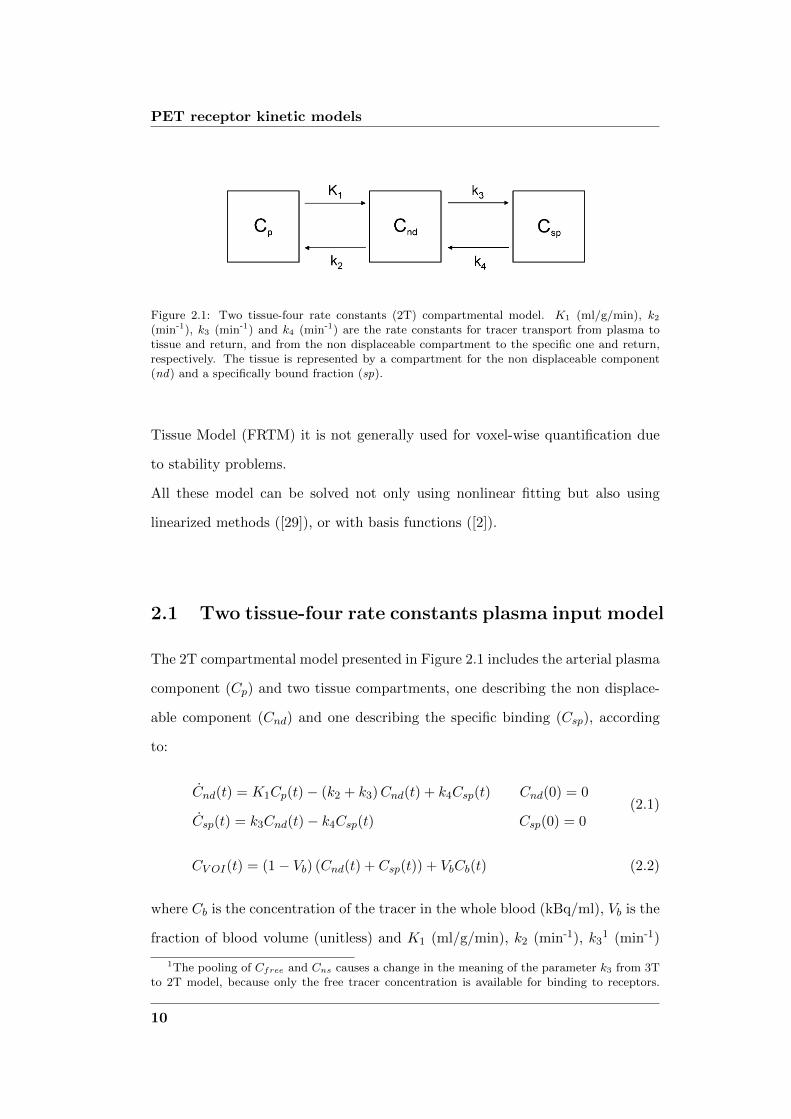
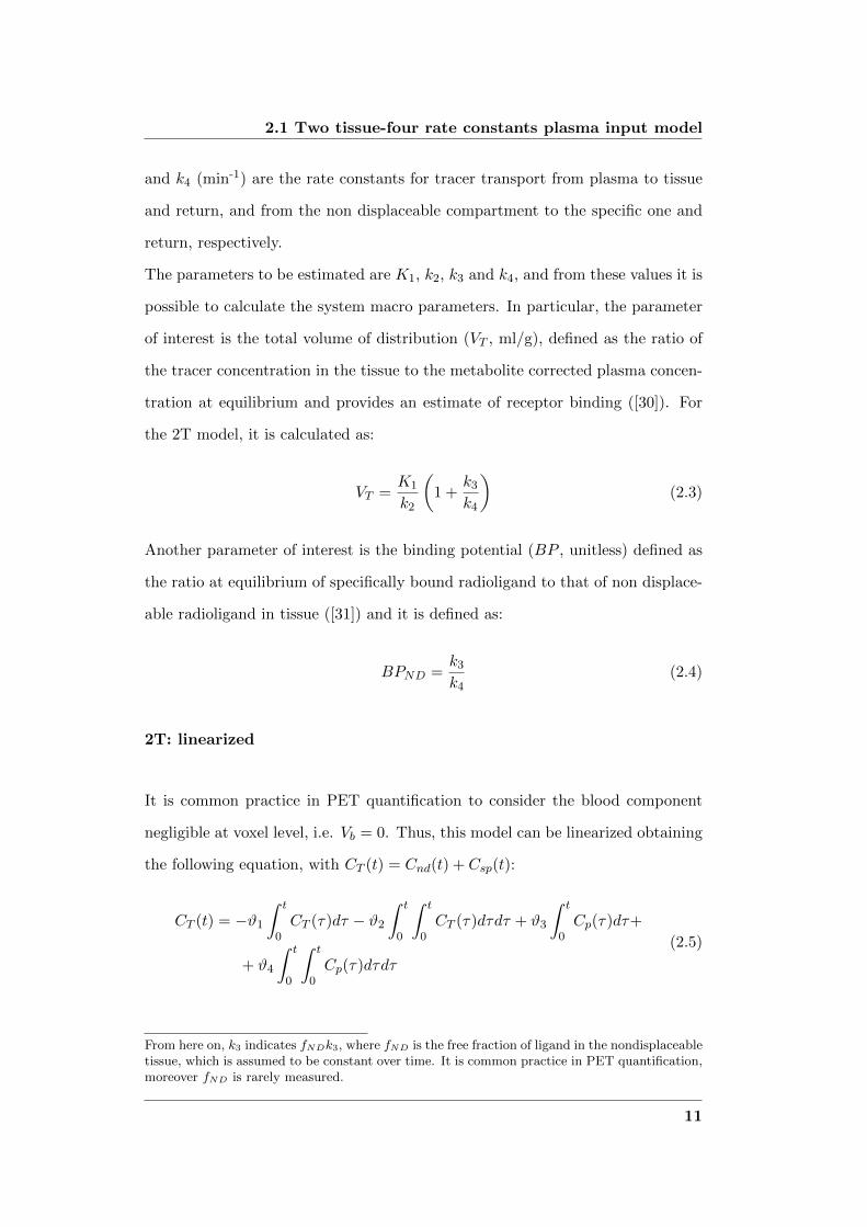
Figure 2.1: Two tissue-four rate constants (2T) compartmental model. K1 (ml/g/min), k2(min-1), k3 (min-1) and k4 (min-1) are the rate constants for tracer transport from plasma totissue and return, and from the non displaceable compartment to the specific one and return,respectively. The tissue is represented by a compartment for the non displaceable component(nd) and a specifically bound fraction (sp).
Tissue Model (FRTM) it is not generally used for voxel-wise quantification due
to stability problems.
All these model can be solved not only using nonlinear fitting but also using
linearized methods ([29]), or with basis functions ([2]).
2.1 Two tissue-four rate constants plasma input model
The 2T compartmental model presented in Figure 2.1 includes the arterial plasma
component (Cp) and two tissue compartments, one describing the non displace-
able component (Cnd) and one describing the specific binding (Csp), according
to:
Cnd(t) = K1Cp(t)− (k2 + k3)Cnd(t) + k4Csp(t) Cnd(0) = 0
Csp(t) = k3Cnd(t)− k4Csp(t) Csp(0) = 0(2.1)
CV OI(t) = (1− Vb) (Cnd(t) + Csp(t)) + VbCb(t) (2.2)
where Cb is the concentration of the tracer in the whole blood (kBq/ml), Vb is the
fraction of blood volume (unitless) and K1 (ml/g/min), k2 (min-1), k31 (min-1)
1The pooling of Cfree and Cns causes a change in the meaning of the parameter k3 from 3Tto 2T model, because only the free tracer concentration is available for binding to receptors.
10
2.1 Two tissue-four rate constants plasma input model
and k4 (min-1) are the rate constants for tracer transport from plasma to tissue
and return, and from the non displaceable compartment to the specific one and
return, respectively.
The parameters to be estimated are K1, k2, k3 and k4, and from these values it is
possible to calculate the system macro parameters. In particular, the parameter
of interest is the total volume of distribution (VT , ml/g), defined as the ratio of
the tracer concentration in the tissue to the metabolite corrected plasma concen-
tration at equilibrium and provides an estimate of receptor binding ([30]). For
the 2T model, it is calculated as:
VT =K1
k2
(1 +
k3k4
)(2.3)
Another parameter of interest is the binding potential (BP , unitless) defined as
the ratio at equilibrium of specifically bound radioligand to that of non displace-
able radioligand in tissue ([31]) and it is defined as:
BPND =k3k4
(2.4)
2T: linearized
It is common practice in PET quantification to consider the blood component
negligible at voxel level, i.e. Vb = 0. Thus, this model can be linearized obtaining
the following equation, with CT (t) = Cnd(t) + Csp(t):
CT (t) = −ϑ1∫ t
0CT (τ)dτ − ϑ2
∫ t
0
∫ t
0CT (τ)dτdτ + ϑ3
∫ t
0Cp(τ)dτ+
+ ϑ4
∫ t
0
∫ t
0Cp(τ)dτdτ
(2.5)
From here on, k3 indicates fNDk3, where fND is the free fraction of ligand in the nondisplaceabletissue, which is assumed to be constant over time. It is common practice in PET quantification,moreover fND is rarely measured.
11

PET receptor kinetic models
with:
ϑ1 = k2 + k3 + k4
ϑ2 = k2k4
ϑ3 = K1
ϑ4 = K1 (k3 + k4)
(2.6)
The parameters ϑ1, ϑ2, ϑ3 and ϑ4 can be estimated with a linear least square
estimator.
2T: basis function
Solving the 2T model, the tissue concentration of Eq. 2.2 can be written in form
of basis functions, with α1, α2 and Vb as parameter to be estimated, as:
CV OI(t) = α1Cp(t)⊗ e−β1t + α2Cp(t)⊗ e−β2t + VbCb(t) (2.7)
where ⊗ denotes the convolution operator and where:
α1 = (1− Vb) K1(β1−k3−k4)β1−β2
α2 = (1− Vb) K1(k3+k4−β2)β1−β2
β1, β2 =(k2+k3+k4)∓
√(k2+k3+k4)2−4k2k42
(2.8)
In this form the model parameters can be estimated with a linear estimator,
assuming β1 and β2 as known, as in [2].
2.2 Two tissue-three rate constants plasma input model
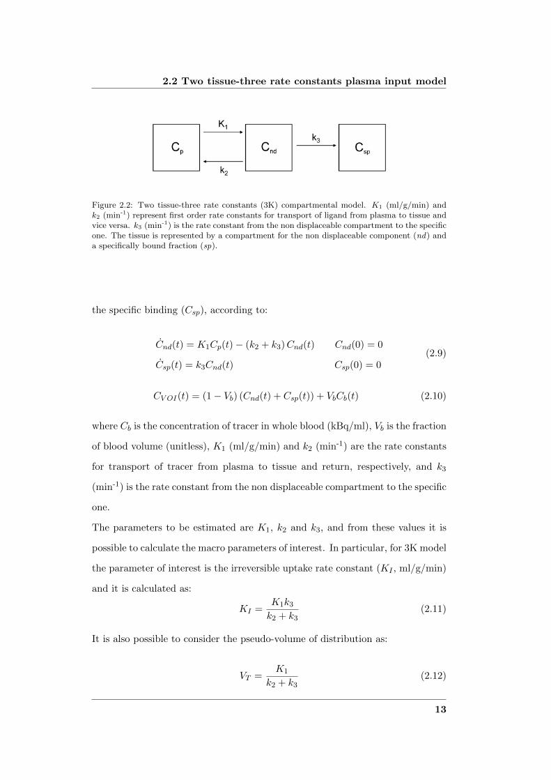
The two tissue-three rate constants compartmental (3K) model was originally
presented in [15], and it is used to describe kinetics of tracers which bind irre-
versibly to the tissue during the PET exam (i.e. k4 = 0). This model (presented in
Figure 2.2) includes the arterial plasma component (Cp) and two tissue compart-
ments, one describing the non displaceable component (Cnd) and one describing
12
2.2 Two tissue-three rate constants plasma input model
Figure 2.2: Two tissue-three rate constants (3K) compartmental model. K1 (ml/g/min) andk2 (min-1) represent first order rate constants for transport of ligand from plasma to tissue andvice versa. k3 (min-1) is the rate constant from the non displaceable compartment to the specificone. The tissue is represented by a compartment for the non displaceable component (nd) anda specifically bound fraction (sp).
the specific binding (Csp), according to:
Cnd(t) = K1Cp(t)− (k2 + k3)Cnd(t) Cnd(0) = 0
Csp(t) = k3Cnd(t) Csp(0) = 0(2.9)
CV OI(t) = (1− Vb) (Cnd(t) + Csp(t)) + VbCb(t) (2.10)
where Cb is the concentration of tracer in whole blood (kBq/ml), Vb is the fraction
of blood volume (unitless), K1 (ml/g/min) and k2 (min-1) are the rate constants
for transport of tracer from plasma to tissue and return, respectively, and k3
(min-1) is the rate constant from the non displaceable compartment to the specific
one.
The parameters to be estimated are K1, k2 and k3, and from these values it is
possible to calculate the macro parameters of interest. In particular, for 3K model
the parameter of interest is the irreversible uptake rate constant (KI , ml/g/min)
and it is calculated as:
KI =K1k3k2 + k3
(2.11)
It is also possible to consider the pseudo-volume of distribution as:
VT =K1
k2 + k3(2.12)
13

PET receptor kinetic models
3K: linearized
Considering negligible the blood component at voxel level, the model can be
linearized obtaining the following equation, with CT (t) = Cnd(t) + Csp(t):
CT (t) = −ϑ1∫ t
0CT (τ)dτ+ϑ2
∫ t
0Cp(τ)dτ + ϑ3
∫ t
0
∫ t
0Cp(τ)dτdτ (2.13)
with:
ϑ1 = k2 + k3
ϑ2 = K1
ϑ3 = K1k3
(2.14)
The parameters ϑ1, ϑ2 and ϑ3 can be estimated with a linear least square esti-
mator.
3K: basis function
This model can be solved with basis functions obtaining the following equation:
CV OI(t) = α0
∫ t
0Cp(τ)dτ + α1Cp(t)⊗ e−β1t + VbCb(t) (2.15)
with:
α0 = (1− Vb) K1k3k2+k3
α1 = (1− Vb) K1k2k2+k3
β1 = k2 + k3
(2.16)
In this form the model parameters α0, α1 and Vb can be estimated with a linear
estimator, assuming β1 as known, as in [2].
2.3 One tissue-two rate constants plasma input model
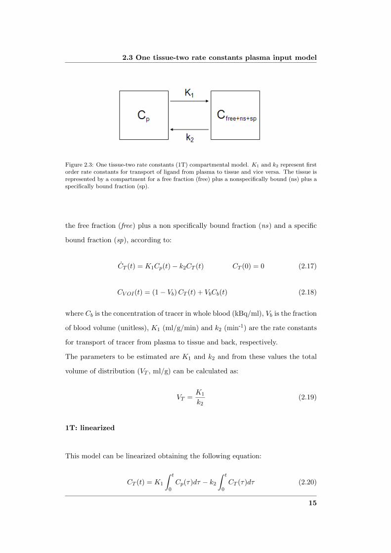
The 1-tissue compartmental (1T) model is the simplest model used to quantify
PET data of reversible tracer. This model (presented in Figure 2.3) includes the
arterial plasma compartment Cp and a tissue compartment CT that incorporates
14
2.3 One tissue-two rate constants plasma input model
Figure 2.3: One tissue-two rate constants (1T) compartmental model. K1 and k2 represent firstorder rate constants for transport of ligand from plasma to tissue and vice versa. The tissue isrepresented by a compartment for a free fraction (free) plus a nonspecifically bound (ns) plus aspecifically bound fraction (sp).
the free fraction (free) plus a non specifically bound fraction (ns) and a specific
bound fraction (sp), according to:
CT (t) = K1Cp(t)− k2CT (t) CT (0) = 0 (2.17)
CV OI(t) = (1− Vb)CT (t) + VbCb(t) (2.18)
where Cb is the concentration of tracer in whole blood (kBq/ml), Vb is the fraction
of blood volume (unitless), K1 (ml/g/min) and k2 (min-1) are the rate constants
for transport of tracer from plasma to tissue and back, respectively.
The parameters to be estimated are K1 and k2 and from these values the total
volume of distribution (VT , ml/g) can be calculated as:
VT =K1
k2(2.19)
1T: linearized
This model can be linearized obtaining the following equation:
CT (t) = K1
∫ t
0Cp(τ)dτ − k2
∫ t
0CT (τ)dτ (2.20)
15
PET receptor kinetic models
The blood component is considered negligible at voxel level, and the parameters
K1 and k2 can be estimated with linear least square estimator.
1T: basis function
This model can be solved with basis functions obtaining the following equation:
CV OI(t) = α1Cp(t)⊗ e−β1t + VbCb(t) (2.21)
with:
α1 = (1− Vb)K1
β1 = k2
(2.22)
In this form the model parameters α1 and Vb can be estimated with a linear
estimator, assuming β1 as known, as in [2].
2.4 Reference Tissue Models
2.4.1 Full Reference Tissue Model
In the Full Reference Tissue Model (FRTM), originally developed in ([20]), the
input function is the TAC of a reference region with non-existent (or very low)
specific binding for the tracer under analysis.
The model was originally implemented at ROI level and it is not generally used
for voxel-wise quantification due to stability problems, even though the model is
globally identifiable.
It is common instead to use the SRTM ([21]), which can be easily implemented
at voxel level using BFM, but it implies a model simplification which leads to loss
of information when the tracer under analysis does not match the assumptions,
i.e. very frequently.
16
2.4 Reference Tissue Models
Figure 2.4: Full Reference Tissue Model (FRTM): K1 (ml/g/min), k2 (min-1), k3 (min-1) and k4(min-1) are the rate constants for tracer transport from plasma to tissue and return, and from thenon displaceable compartment to the specific one and return, respectively. K′1 (ml/g/min) andk′2 (min-1) are the rate constant for transfer from plasma to reference compartment and return,respectively. The tissue is represented by a compartment for the non displaceable component(nd) and a specifically bound fraction (sp).
The FRTM presented in Figure 2.4 includes the arterial plasma component (Cp),
two tissue compartments, one describing the non displaceable component (Cnd)
and one describing the specific binding (Csp), and one reference component (Cr).
The blood component is considered negligible. The model is based on the follow-
ing differential equations:
Cr(t) = K ′1Cp(t)− k′2Cr(t) Cr(0) = 0
Cnd(t) = K1Cp(t)− (k2 + k3)Cnd(t) + k4Csp(t) Cnd(0) = 0
Csp(t) = k3Cnd(t)− k4Csp(t) Csp(0) = 0
(2.23)
CV OI(t) = Cnd(t) + Csp(t) (2.24)
where K1 (ml/g/min), k2 (min-1), k3 (min-1) and k4 (min-1) are the rate constants
for transfer from plasma to tissue and return, and from the non displaceable
compartment to the specific one and return, respectively. K ′1 (ml/g/min) is the
rate constant for transfer from plasma to reference compartment and k′2 (min-1)
is the rate constant for transfer from reference to plasma compartment.
17

PET receptor kinetic models
The parameter of interest is the binding potential (BP , unitless) defined as the
ratio at equilibrium of specifically bound radioligand to that of non displaceable
radioligand in tissue ([31]) and it is defined as:
BP =k3k4
(2.25)
The model described by Eq. 2.23 is not univocally identifiable as the rate con-
stants K1 and K ′1 only enter as a ratio (R1 = K1K′1
), accounting for differences in
delivery between the region of interest and the reference tissue. Assuming that
the volume of distribution of the not specifically bound tracer in both tissues is
the same, i.e.:
K ′1k′2
=K1
k2(2.26)
k′2 can be replaced by k2/R1, and the model becomes identifiable. Thus the model
parameters are R1, k2, k3 and k4.
FRTM: linearized
The FRTM can be linearized obtaining the following equation:
CV OI(t) = −ϑ1∫ t
0CT (τ)dτ − ϑ2
∫ t
0
∫ t
0CT (τ)dτdτ + ϑ3
∫ t
0Cr(τ)dτ+
+ ϑ4
∫ t
0
∫ t
0Cr(τ)dτdτ + ϑ5Cr(t)
(2.27)
with:
ϑ1 = k2 + k3 + k4
ϑ2 = k2k4
ϑ3 = (k2 −R1k2)
ϑ4 = (k2k3 + k4 (k2 −R1k2))
ϑ5 = R1
(2.28)
The parameters ϑ1, ϑ2, ϑ3, ϑ4 and ϑ5 can be estimated with a linear least square
estimator.
18
2.4 Reference Tissue Models
Figure 2.5: Simplified Reference Tissue Model (SRTM): K1 (ml/g/min) and k2a (min-1) are therate constants for tracer transport from plasma to tissue and return. K′1 (ml/g/min) and k′2(min-1) are the rate constant for transfer from plasma to reference compartment.
FRTM: basis functions
From the assumption described above, it is possible to obtain the 2.23 in basis
function form, as:
CV OI(t) = R1Cr(t) + α1Cr(t)⊗ e−β1t + α2Cr(t)⊗ e−β2t (2.29)
with:
α1 = (β1−k3−k4)(k2/R1−β1)β1−β2
α2 = (k3+k4−β2)(k2/R1−β2)β1−β2
β1, β2 =(k2+k3+k4)∓
√(k2+k3+k4)2−4k2k42
(2.30)
where R1, α1 and α2 can be estimated with a linear estimator, assuming β1 and
β2 as known, as in [2].
2.4.2 Simplified Reference Tissue Model
SRTM can be used when one compartment can reasonable describe the kinetics
of the tracer in tissue ([21]). The SRTM presented in Figure 2.5 includes the
19
PET receptor kinetic models
arterial plasma component (Cp), one tissue compartment (CT ) that incorporated
the non displaceable fraction (nd) and a specific bound fraction (sp), and one
reference component (Cr). The vascular component is considered negligible.
The model is based on the following differential equations:
Cr(t) = K ′1Cp(t)− k′2Cr(t) Cr(0) = 0
CT (t) = K1Cp(t)− k2aCT (t) CT (0) = 0(2.31)
where K ′1 is the rate constant for transfer from plasma to reference compartment
(ml/g/min) and k′2 is the rate constant for transfer from reference to plasma
compartment (min-1). K1 (ml/g/min) and k2a (min-1) are the rate constants for
tracer transport from plasma to tissue and return, and k2a = k21+BP , with BP
defined as in 2.25.
The parameters of the simplified model to be estimated are R1, k2 and BP .
SRTM: linearized
The SRTM can be linearized obtaining the following equation:
CT (t) = −ϑ1∫ t
0CT (τ)dτ + ϑ2
∫ t
0Cr(τ)dτ + ϑ3Cr(t) (2.32)
with:
ϑ1 = k21+BP
ϑ2 = k2
ϑ3 = R1
(2.33)
The parameters ϑ1, ϑ2 and ϑ3 can be estimated with a linear least square esti-
mator.
20

2.4 Reference Tissue Models
SRTM: basis functions
The SRTM model is generally solved using basis functions, as described originally
in [2]:
CT (t) = R1Cr(t) + α1Cr(t)⊗ e−β1t (2.34)
with:
α1 =[k2 − k2R1
1+BP
]β1 = k2
1+BP
(2.35)
In this form the model parameters R1 and α1 can be estimated with a linear
estimator, assuming β1 as known, as in [2].
21


Chapter 3
Novel approaches for Bayesian
voxel-wise PET quantification
3.1 Bayesian PET modeling
The principle of Bayesian statistics is to incorporate prior knowledge about un-
known model parameters in the estimation process, along with a given set of
measured data.
In this context, the expression ”Bayesian methods” is used when any kind of a
priori information on the parameters is assumed known and used for the esti-
mation. This knowledge can be obtained from operational or observational data,
from previous comparable experiments or from physiological knowledge. When
the prior information is derived from the data, the method is referred to as em-
pirical Bayes.
The output of a generic dynamic system can be described in vectorial form by
y = g(p, t) + v (3.1)
where g(p, t) represents the dynamic model of the system with m unknown pa-
rameters p = [p1, p2, . . . , pm]T and y is the n-dimensional vector containing the
23

Novel approaches for Bayesian voxel-wise PET quantification
measures collected at times t1, t2, . . . , tn. The measures are affected by an addi-
tive error v which is assumed to be a zero mean Gaussian vector made of random
variables v1, v2,. . . , vn.
For the sake of simplicity the explicit dependence on time will be omitted, i.e.
instead of indicating the function of m parameters pi as g(p, t), the simpler g(p)
will be employed.
In the Bayesian approach, a probability density function fp(p) is associated to
the unknown parameter vector p and it is assumed known.
It is possible to define the probability density function of the parameters vector
given the data (called a posteriori distribution):
fp|y (p |y) (3.2)
that, according to Bayes’ rule, can be written as:
fp|y (p |y ) =fy|p (y |p)fp(p)
fy(y)(3.3)
where fy(y) is the prior probability density function of the measurements vector
y.
Maximum a Posteriori (MAP) estimator derives the estimates by maximizing Eq.
3.3:
pMAP = arg maxp
fp|y (p |y) (3.4)
where arg max stands for the argument of the maximum.
Using Bayes’ rule and as fy(y) is independent from p, the MAP estimator can
be described as:
pMAP = arg maxp
fy|p (y |p) fp(p) (3.5)
The expression for fy|p (y |p) is simplified considerably if specific assumptions
regarding the distributions of v, fv(v), p and fp(p) are made. For instance, let
24
3.1 Bayesian PET modeling
us assume that both v and p are independent and normally distributed. Then:
pMAP = arg min [y −G(p)]T Σ−1v [y −G(p)] + (p− µp)−1 Σ−1p (p− µp) (3.6)
where G(p) indicates the structural model of the system, z the vector of the
measured data, Σv the covariance matrix of the measurement error, p the vector
of the model parameters. µp and Σp are, respectively, the mean and covariance
of the prior probability of p.
This prior information is updated from the observed data, generating the a pos-
teriori probability density function. Thus the MAP estimator realizes a compro-
mise between the a priori and a posteriori information.
As said, the Bayesian methods require an assumption on the a priori probability
distribution of p.
It is common practice in PET modeling to use the terms ”Bayesian” and ”prior” in
a wider sense: not only when a priori information is available on the probability
density function of the unknown parameter vector itself, but also when it is
possible to obtain some kind of a a priori knowledge on the tracer kinetics. This
was the approach used and developed in Section 3.3.
In Bayesian methods for quantitative PET, the major problem is how to derive
the a priori knowledge, i.e. µp and Σp (mean and covariance of p), because there
is not a unique way.
The a priori information can be derived from in vitro data, or from literature, or
as in [7] from a previous voxel-based analysis of subjects sharing similar charac-
teristics using the mean and standard deviation (SD) value of the voxel estimates
to represent the a priori probability of the parameters of each voxel of the subject
under analysis.
An alternative approach is to assume that the voxels belonging to a ROI have
to share similar proprieties and will have estimates similar to those obtained by
25
Novel approaches for Bayesian voxel-wise PET quantification
using the mean TAC derived from the ROI itself. This is not a novel approach
but it can be found in [6], [32] and [33] where the voxel is considered as an in-
dividual in a population and assuming that it shares certain characteristics with
the other individuals belonging to the same population (i.e. the ROI).
Consequently the priors are different for each subject of the dataset, and moreover
they are different for each ROI and they allow taking into account the inter-ROI
variability.
The proposed approaches are both developed following a multi-stage hierarchical
scheme where, starting from the kinetic analysis of the whole brain, information
is cascaded to anatomical systems that are akin in terms of receptor densities,
and then down to the voxel level.
A priori classes of voxels are generated either by anatomical atlas segmentation
or by functional segmentation using unsupervised clustering.
The anatomical atlas is a standardized space where each voxel is labeled to the
ROI which it is more likely to belong to. The regions are already defined and
they can be applied easily to PET images. The atlas used for this work was the
Maximum Probability Hammersmith BrainAtlas, developed by [27], made avail-
able by the Imperial College.
To extract functional information, various algorithms were implemented. For the
majority of the tracer the k-means partitioning method ([34]), widely used for
pattern recognition, was appropriate for the ROI definition.
In alternative, the Fuzzy C-Means partitioning method ([35], [36]) was consid-
ered, in its original version or combined with k-means method (details given in
Section 4.2 and Chapter 5).
A representation of the hierarchical process is presented in Figure 3.1. The PET
image was segmented using either anatomical or functional information. For each
26

3.1 Bayesian PET modeling
Figure 3.1: Pipeline describing the hierarchical process. The PET image is segmented usingeither anatomical or functional information. The ROI TACs are extracted from the regions(or clusters) and the optimal model used to describe the data is solved for each ROI withWNLLS. From the ROI estimates pi, one set of prior is defined for each region with µp = pi
and Σp = diag(σ2pi
). The voxel-wise analysis is then implemented, using as prior the one definedfor the region which the voxel belongs to.
ROI (ROI1, ROI2, . . . , ROIT , with T number of region which the brain was seg-
mented into) the mean TAC was extracted from the regions (or clusters) and the
optimal model used to describe the data was solved with a weighted nonlinear
least square estimator (WNLLS). From the ROI analysis, one set of estimated
parameter vectors was obtained for each region (i.e., pi), and from these values
one set of priors was defined for each region with µp = pi and Σp = diag(σ2pi).
The voxel-wise analysis was then implemented, using as prior the one defined for
27
Novel approaches for Bayesian voxel-wise PET quantification
the region which the voxel belongs to.
3.2 Hierarchical Maximum a Posteriori (H-MAP)
Hierarchical MAP is a new hierarchical approach for the generation of PET para-
metric maps where the estimates are obtained using a linear MAP estimator ap-
plied at the voxel level. The method can be applied to any linear or linearized
PET model described in Chapter 2. The priors for the Bayesian estimator are gen-
erated automatically from the data, and as a consequence are user-independent.
As described in Chapter 3, H-MAP requires at first the model to be solved at
the ROI level. For each region, the mean TAC is extracted and the model is
identified with a non linear estimator, which represents the gold standard.
The model is then linearized and solved at voxel level using the MAP estimator
of Eq. 3.6 to account for the bias introduced with the linearization of the model.
The solution of Eq. 3.6 for a linear model leads to a closed form ([37], [38]):
pMAP =(GTΣ−1v G + Σ−1p
)−1 (GTΣ−1v CT + Σ−1p µp
)(3.7)
where CT is the nx1 vector with the noisy measures, G(p) is the predicted model
output with size depending on the model used, n is the number of the tissue
measures. The measurement error is assumed to be additive, uncorrelated, from
a Gaussian distribution with zero mean and covariance matrix Σv, a nxn diagonal
matrix estimated a posteriori, according to a relative weighting scheme, where
Σv is known less than a scale factor γ ([39], [40]). p is the unknown parameter
vector having a normal prior probability with mean µp and covariance matrix Σp,
which is defined diagonal.
The prior knowledge (i.e. µp and Σp) is extracted from the PET data. The
28
3.3 Hierarchical Basis Function Method (H-BFM)
estimates obtained at ROI level are used to define one set of priors for the MAP
estimator for each region. The mean µp of the normal prior distribution is set
equal to the estimates obtained with WNLLS for the mean TAC.
The covariance matrix Σp is calculated directly from the standard deviation of
the accuracy of the WNLLS estimates. The accuracy relates the variability of
the estimates to the expected variability of the measurements. Thus, its value is
assumed to represent the uncertainty associated with µp.
3.3 Hierarchical Basis Function Method (H-BFM)
Hierarchical Basis Funtion Method (BFM) is a new hierarchical method for PET
quantification to apply BFMs to mono- and multi-compartmental models. The
method allows to solve the compartmental model at voxel level in its non linear
version, overcoming the limitations related to the grids described in Chapter 1,
making them user-independent and subject and ROI specific.
This method is considered a Bayesian approach in PET, even if it does not rely
on a Bayesian estimator, because additional information are added to the data
to be analyzed. In particular, the grids used to create the basis functions for
the analysis at voxel level are defined from the information obtained solving the
model at ROI level, in a hierarchical top-down approach. Consequently, even if
the a priori knowledge is not on the actual parameters to be estimated, the grid
selection implies to determinate an interval of physiologically plausible values.
As for H-MAP, following Chapter 3, at first the model is solved at the ROI
level for each region with a non linear estimator (gold standard).
For each time frame (i = 1,. . . , n, with n number of frames), basis functions can
be pre-calculated for the non linear terms involving Cp(t) (or Cr(t), if a reference
29
Novel approaches for Bayesian voxel-wise PET quantification
input model is considered) as:
Bjl(ti) = Cp(ti)⊗ e−βjlti l = 1, . . . ,M (3.8)
with M number of elements of the grid, j = 1 for 1T and 3K model and j = 2
for 2T model.
The local grids for the basis functions for the voxel-by-voxel analysis are defined
a priori, generated automatically from the data, specifically for each ROI, from
the estimates obtained with the ROI analysis.
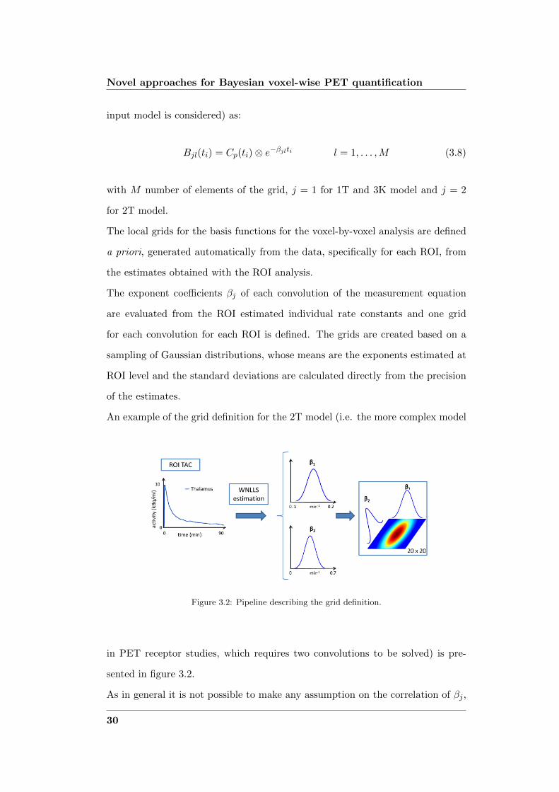
The exponent coefficients βj of each convolution of the measurement equation
are evaluated from the ROI estimated individual rate constants and one grid
for each convolution for each ROI is defined. The grids are created based on a
sampling of Gaussian distributions, whose means are the exponents estimated at
ROI level and the standard deviations are calculated directly from the precision
of the estimates.
An example of the grid definition for the 2T model (i.e. the more complex model
Figure 3.2: Pipeline describing the grid definition.
in PET receptor studies, which requires two convolutions to be solved) is pre-
sented in figure 3.2.
As in general it is not possible to make any assumption on the correlation of βj ,
30

3.3 Hierarchical Basis Function Method (H-BFM)
the grids are defined 2-dimensional. Consequently the size of the grids is to be
chosen appropriately, such a way to not be too computational demanding, but to
give enough information to describe the data.
The model expressed in basis functions is then solved with linear least squares
for each element of the grids, calculating the Weighted Residual Sum of Squares
(WRSS), as in [2]:
WRSSl =∑n
i=1wi [CT (ti)− Cl(ti)]2 (3.9)
where CT is the nx1 vector of the measures, wi is the inverse of the measurement
error variance and Cl is the model output for the lth element of the grids. The
best solution is the one which minimizes WRSS and the individual kinetic rate
constants are calculated from the estimated αj .
31


Chapter 4
Image Acquisition and
Processing
4.1 Datasets and Processing
4.1.1 [11C]DPN (Opioid receptor ligand)
[11C]DPN is a reversible non-subtype selective antagonist at opioid receptors and
has often been used, mainly in studies of pain, neurodegeneration, epilepsy and
addiction ([41]). It has high affinity at µ, κ and δ opioid receptors ([42], [43]),
being an antagonist at µ and δ subtypes, but has a weak efficacy at the κ opioid
receptor, where it acts as a partial agonist ([44]).
[11C]DPN has rapid cerebral uptake and in humans, in vivo, it has high uptake
in regions such as thalamus, temporal, frontal, and parietal cortices, which are
known from post mortem studies to have high concentrations of µ, κ and δ opi-
oid receptors ([42]). Relative to the duration of a PET study, [11C]DPN has very
slow kinetics, with binding close to irreversible, representing a challenge to the
estimation of the parameters of interest, particularly at the voxel level.
33

Image Acquisition and Processing
PET studies
Data from previously reported studies ([45]) of five healthy control subjects (each
of them scanned twice) were made available by the Imperial College. The criteria
for subject inclusion and the procedure for [11C]DPN PET studies are described
in detail in [45]. Briefly, all subjects underwent paired 90-min dynamic [11C]DPN
PET test-retest scans on a Siemens/CTI ECAT EXACT3D PET camera. Ac-
quisition was performed in list-mode (event by event) and scans were rebinned
into 32 time frames of increasing duration (variable length background frame, 3
x 10s, 7 x 30 s, 12 x 120 s, 6 x 300 s, 3 x 600 s).
The subjects were positioned optimally within the field of view and thirty seconds
after the scan start they were injected with ∼ 185 MBq (185 ± 4, range 181 - 191)
of [11C]DPN over a total of 30 s. Data were reconstructed using the reprojection
algorithm ([46]) and then corrected for movement. The reconstructed voxel sizes
were 2.096 mm x 2.096 mm x 2.43 mm.
Arterial blood was continuously withdrawn at a sampling rate of 5 ml/min for
the first 15 min, then discrete blood samples were taken in all subjects for cross
calibration and for determination of blood radioactivity at 5, 10, 15, 20, 30, 40,
50, 60, 75 and 90 min after start of scan. Seven of these samples were also used for
quantification of the fraction of radioactivity attributable to unmetabolized par-
ent radiotracer, generating the metabolite-corrected arterial plasma input func-
tion for all subjects.
The tissue, blood and plasma data were corrected for decay of 11C.
Anatomical ROI segmentation
Each subject also had high-resolution 3D T1 weighted MR scans. The MRI data
sets were used only for region definition, using Statistical Parametric Mapping
(SPM8, Wellcome Department of Imaging Neuroscience, Institute of Neurology,
34

4.1 Datasets and Processing
UCL, London, UK), running under Matlab R©(The Mathworks Inc., Natick, MA,
USA).
An individualized Maximum Probability Hammersmith Brain Atlas ([27]), based
on thirty atlas data sets subdivided into 83 anatomical regions each ([47]) in
standard stereotaxic space (MNI/ICBM 152), was created for every subject and
provided already in the individual MRI space. The rigid transformation for MRI-
to-PET coregistration was then derived from SPM8’s normalized mutual informa-
tion option ([48]) and applied to the original MRI and the transformed maximum
probability atlas, resulting in all the images being in register with the given un-
changed PET image data set. Finally the atlas was multiplied in PET space and
the 83 ROIs TACs were derived, obtained meaning the voxel TACs belonging to
each of the 83 anatomical regions.
The regions were chosen following previous studies ([49], [45]): one small central
structure with high opioid receptor density (thalamus), one larger region from
the frontal cortex with intermediate signal (inferior frontal gyrus), two regions
with low signal (cerebellum and brainstem), one region from the occipital cor-
tex with minimal receptor density (lingual gyrus), one small anisotropic region
with special interest in epileptology and memory research (hippocampus) and
another small region among the central structures (putamen). For comparison
with previous published data left and right regions combined were considered.
4.1.2 [11C]FLB457 (Dopamine receptor ligand)
[11C]FLB457 is a radioligand for quantification of dopamine D2/D3 receptor bind-
ing in extrastriatal brain regions and it is used mostly in research studies on
neuropsychiatric disorders.
Extrastriatal dopamine receptors have since long been proposed as targets for
antipsychotic drugs ([50]) and neuroimaging and pharmacological evidence has
supported the view that limbic cortical dopamine D2/D3 receptors may be the
main target of antipsychotic medication ([51], [52], [53]).
35

Image Acquisition and Processing
Quantification of dopamine receptors in extrastriatal regions is generally ham-
pered by the low receptor density which in most such regions is 1 to 10% of that
in the striatum ([54]), thus it is necessary a radioligand with very high affinity to
accurately measure small receptor densities in regions that can also have small
volume.
[11C]FLB457 is a substituted benzamide with very high affinity for D2/D3 dopami-
ne receptors, whereas the affinity to other putative central receptors is negligible
([55]). It can be used to visualize and quantify low density dopamine receptor
populations in the human brain and the distribution of radioactivity is consistent
with the known distribution of dopamine D2/D3 receptors ([54]).
PET studies
Data from previously reported studies ([56]) of four depressed subjects were made
available by the Imperial College. The criteria for subject inclusion and the pro-
cedure for [11C]FLB457 PET studies are described in detail in [56].
Briefly, four depressed subjects underwent a 90-min dynamic PET study in a CTI
ECAT EXACT3D tomography after a bolus injection of 280 MBq to 380 MBq of
[11C]FLB 457. All PET data were acquired in 3-dimensional mode, corrected for
attenuation, detector efficiency, random events, and scatter, and reconstructed
into tomographic images using filtered back-projection.
Acquisition was performed in list-mode (event by event) and scans were rebinned
into 32 time frames of increasing duration (variable length background frame, 9
x 10 s, 4 x 30 s, 2 x 60 s, 2 x 120 s, 1 x 180 s, 10 x 300 s, 3 x 600 s). The
reconstructed voxel sizes were 2.096 mm x 2.096 mm x 2.43 mm.
After injection of [11C]FLB457 the radioactivity concentration in blood was mea-
sured continuously and in addition serial discrete blood samples were taken at
increasing time intervals throughout the study for the measurement of the ra-
dioactivity in blood and plasma. Eight of these samples were also used for quan-
tification of the fraction of radioactivity attributable to unmetabolized parent
36

4.1 Datasets and Processing
radiotracer, generating the metabolite-corrected arterial plasma input function
for all subjects.
The tissue, blood and plasma data were corrected for decay of 11C.
Anatomical ROI segmentation
Each subject also had high-resolution 3D T1 weighted MR scans. The MRI data
sets were used only for region definition, using SPM8, running under Matlab.
A Maximum Probability Brain Atlas ([27]) subdivided in 73 regions defined in
standard stereotaxic space (MNI/ICBM152) was used to define the ROI. The
MR MNI template was normalized to each subject’s MR image using SPM8 and
the atlas was applied to the subject’s MR space by applying the normalization
parameters. Then for each subject, the MRI was coregistered to the summed
PET using SPM8, with normalized mutual information option ([48]) and the
normalization parameters were applied to the transformed maximum probability
atlas, resulting in all the images being in register with the given unchanged PET
image data set. Finally the atlas was multiplied in PET space and the 73 ROIs
TACs were derived, obtained meaning the voxel TACs belonging to each of the
73 anatomical regions.
Following previous studies ([54]) the hippocampus, amygdale, cerebellum, thala-
mus, frontal cortex, temporal cortex and anterior cingulate were selected. The
right and left hemispheres were considered combined.
The striatum was not considered because the study duration was shorter than
the time required to reach equilibrium in this D2/D3 receptor-rich region ([57]).
37

Image Acquisition and Processing
4.1.3 [11C]WAY100635 (Serotonin receptor ligand)
[11C]WAY100635 (from here on, [11C]WAY100635 indicates [carbonyl -C11]WAY-
100635) is a selective antagonist with high affinity and selectivity for serotonin
5HT1A receptors, which are of central interest in research on the pathophysiology
and treatment of psychiatric disorders ([58], [59]).
[11C]WAY100635 provides high-contrast delineation of brain regions that are rich
in 5-HT1A receptors ([60]) It shows rapid clearance of the compound from the
cerebellum and high uptake in cortical and raphe regions. It also presents rapid
clearance from plasma [61].
PET studies
A dataset of four healthy male subjects was made available by the Imperial Col-
lege. Each subject underwent a 90-min dynamic PET study in a CTI ECAT
EXACT3D tomography after a bolus injection of [11C]WAY 100635. All PET
data were acquired in 3-dimensional mode, corrected for attenuation, detector ef-
ficiency, random events, and scatter, and reconstructed into tomographic images
using filtered back-projection.
Acquisition was performed in list-mode (event by event) and scans were rebinned
into 23 time frames of increasing duration (two variable length background frame,
3 x 5 s, 2 x 15 s, 4 x 60 s, 7 x 300 s, 5 x 600 s). The reconstructed voxel sizes
were 2.096 mm x 2.096 mm x 2.43 mm.
After injection of [11C]WAY100635 , the radioactivity concentration in blood was
measured continuously and in addition serial discrete blood samples were taken
at increasing time intervals throughout the study for the measurement of the ra-
dioactivity in blood and plasma. Nine of these samples were also used for quan-
tification of the fraction of radioactivity attributable to unmetabolized parent
radiotracer, generating the metabolite-corrected arterial plasma input function
38

4.1 Datasets and Processing
for all subjects.
The tissue, blood and plasma data were corrected for decay of 11C.
Anatomical ROI segmentation
Each subject also had high-resolution 3D T1 weighted MR scans. The MRI data
sets were used only for region definition, using SPM8, running under Matlab.
As for the dataset of [11C]FLB 457, a Maximum Probability Brain Atlas ([27])
subdivided in 73 regions was used to define the ROI, with the same procedure as
in Section 4.1.2. The atlas was registered on PET space as described above and
the 73 ROIs TACs were derived, obtained meaning the voxel TACs belonging to
each of the 73 anatomical regions. The ROIs were selected on the base of previ-
ous studies: cerebellum, thalamus as region with low binding and insula cortex,
cingulate cortex, frontal cortex, raphe nucleus, temporal cortex as regions rich of
5HT1A receptor ([62]). Right and left hemispheres were considered combined.
4.1.4 [11C]SCH442416 (Adenosine receptor ligand)
[11C]SCH442416 is a nonxanthine radioligand which binds selectively and re-
versibly to striatal A2A receptors, which are abundant in basal ganglia, vascu-
lature and platelets ([63]). A2A receptor interacts structurally and functionally
with the dopamine D2 receptor and this interaction is of particular interest as
it is thought to be central to basal ganglia dysfunction in Parkinson’s disease.
([64]).
Preclinical studies on rats and nonhuman primates suggest that [11C]SCH442416
is suitable for the in vivo imaging of adenosine A2A receptors with PET because
of its high affinity and selectivity, good signal-to-noise ratio, and low levels of
radioactive metabolites in the brains ([63],[65]).
To the author’s knowledge, there are only few previous works where [11C]SCH-
442416 data were analyzed in humans: in [66] data from 15 healthy subjects were
39
Image Acquisition and Processing
analyzed with kinetic modeling, to demonstrate the efficacy of vipadenant as po-
tential treatment of Parkinson’s disease. In [67] and [68] 4 normal subjects and 12
patients with Parkinson’s disease with and without levodopa-induced dyskinesia
respectively were studied with spectral analysis.
Nevertheless a proper analysis to identify the optimal compartmental model to
describe the data has never been carried out. A preliminary work was proposed
in [69] in which both data- and model-driven methods were used.
PET studies
Data of [11C]SCH442416 of six healthy subjects were made available by the Im-
perial College. Each subject underwent a 90-min dynamic PET scanning in a
Siemens ECAT EXACT HRD scanner after a bolus injection of an average of
612 MBq of [11C]SCH442416 over 10 seconds, 30 seconds after the start of the
scan. All PET data were acquired in 3-dimensional mode, corrected for atten-
uation, detector efficiency, random events, and scatter, and reconstructed into
tomographic images using filtered back-projection.
Acquisition was performed in list-mode (event by event) and scans were rebinned
into 34 time frames of increasing duration (variable length background frame, 6
x 10s, 3 x 20s, 3 x 30s, 4 x 60s, 6 x 120s, 8 x 300s, 3 x 600s). The reconstructed
voxel sizes were 2.096 mm x 2.096 mm x 2.43 mm.
After injection of [11C]SCH442416 the radioactivity concentration in blood was
measured continuously for the first 15 minutes with discrete blood samples taken
at baseline, 5, 10, 15, 20, 30, 40, 50, 60, 75, and 90 minutes. Eight of these sam-
ples were also used for quantification of the fraction of radioactivity attributable
to unmetabolized parent radiotracer, generating the metabolite-corrected arterial
plasma input function for all subjects.
The tissue, blood and plasma data were corrected for decay of 11C.
40

4.1 Datasets and Processing
Anatomical ROI segmentation
Each subject had a volumetric T1-weighted MRI performed with a Philips 1.5 T
Eclipse system. The MRI data sets were used only for region definition, using
SPM8, running under Matlab.
The same procedure used for [11C]FLB457 and [11C]WAY100635 data as in Sec-
tion 4.1.2 was also applied for the ROI segmentation for this dataset. A Maximum
Probability Brain Atlas ([27]) subdivided in 73 regions was registered on PET
space as described above and the 73 ROIs TACs were derived, obtained meaning
the voxel TACs belonging to each of the 73 anatomical regions.
The ROIs selected for the analysis were cerebellum, thalamus, frontal and tempo-
ral cortices, anterior cingulate, pallidum and striatum. Right and left hemispheres
were considered combined.
4.1.5 [11C]MDL100907 (Serotonin receptor ligand)
[11C]MDL100907 is a high affinity PET ligand which allowed an improvement in
the in vivo quantification of 5-HT2A receptor, which has been localized through-
out the brain, including cortical regions, prefrontal cortex, caudate nucleus, nu-
cleus accumbens, olfactory tubercle and hippocampus ([70]).
Previous studies with [11C]MDL100907 have revealed high-quality images of re-
ceptor availability, which correspond well with the known distribution of 5-HT2A
binding sites from post-mortem studies ([71], [72]). [11C]MDL100907 is a com-
petitive antagonist with subnanomolar affinity for 5-HT2A receptor at least 100
times higher than the affinity for the other 5-HT receptors. Imaging studies in
man have shown that it binds specifically to 5-HT2A receptors with high specific
to nonspecific binding ([73]). The 5-HT2A receptor has been implicated in the
pathophysiology of various neuropsychiatric disorders, including schizophrenia,
major depression, anxiety, sleep disorders and Obsessive Compulsive Disorder
41
Image Acquisition and Processing
(OCD) ([74], [75], [76]). Both postmortem and brain imaging studies have evi-
denced the role of 5-HT2A receptor in the pathophysiology of depressive illness
and in the action of antipsychotics ([77]).
PET studies
We analyzed [11C]MDL100907 binding to 5-HT2A receptors in vivo in two dif-
ferent datasets, made available by Imperial College of London (UK) and by San
Raffaele Scientific Institute (HSR) of Milan (Italy).
Imperial dataset Data from previously reported studies ([78]) of six healthy
control subjects were used in the current study. The criteria for subject inclusion
and the procedure for [11C]MDL100907 PET studies are described in detail in
[78]. Briefly, six healthy subjects undergone twice a 90-min PET scan in a ECAT
EXACT3D scanner following injection of 361 MBq of [11C]MDL100907 (under
baseline condition and after administration of a single dose of mirtazapine, a
5-HT2A blocking). Mirtazapine is an antidepressant, which acts by blocking 5-
HT2A/2C and 5-HT3 receptors ([79]).
For all the PET exams at baseline plasma input functions were available. Only
for one subject the plasma input function was available after administration of
mirtazapine, consequently it was used only as case study and to validate the effect
of the blockade on the tracer binding. Acquisition was performed in list-mode
(event by event) and scans were rebinned into 28 time frames of increasing du-
ration (30 s background frame before injection, then 3 x 10 s, 3 x 20 s, 3 x 30 s,
3 x 60 s, 4 x 120 s, 6 x 300 s and 5 x 600 s). The reconstructed voxel sizes were
2.096 mm x 2.096 mm x 2.43 mm.
Arterial whole-blood activity was continuously withdrawn for the first 15 min
then discrete blood samples were taken in all subjects at 5, 10, 15, 20, 30, 40, 50,
60, 75 and 95 min. Eight of these samples were also used for quantification of the
42
4.1 Datasets and Processing
fraction of radioactivity attributable to unmetabolized parent radiotracer, gener-
ating the metabolite-corrected arterial plasma input function for all subjects.
The tissue, blood and plasma data were corrected for decay of 11C.
HSR dataset HSR dataset consisted in both healthy subjects and drug-naıve
OCD patients. In particular, 6 healthy subjects, 3 of them scanned twice in base-
line condition, and 12 OCD patients, scanned twice (baseline condition and after
administration of fluvoxamine) were available. Fluvoxamine is a potent Selective
Serotonin Reuptake Inhibitor (SSRI) with high affinity for the serotonin trans-
porters and negligible affinity for the dopamine transporter or any other receptor.
Plasma input functions were available for four of the healthy subjects for the first
PET exam.
All subjects underwent a 90-min PET in a GE Advance scanner after injection
of 190 to 370 MBq of [11C]MDL100907 . After tracer injection, 17 sequential of
increasing length were acquired (4 x 60 s, 3 x 120 s, 6 x 300 s, 2 x 600 s, 2 x
900 s). Trans-axial images were reconstructed using a Shepp-Logan filter (cut-off
5 mm filter width) in the transaxial plane, and a Shepp-Logan filter (cut-off 8.5
mm) in the axial direction. The reconstructed voxel sizes were 2.5 mm x 2.5 mm
x 4.25 mm.
Twenty discrete blood samples were manually taken in 4 healthy subjects at spe-
cific times: 10 samples at close range until 1 min, then at 3, 5, 10, 20, 30, 40, 50,
60, 75 and 90 min. The concentration of the tracer in the plasma uncorrected for
the metabolites was generated. Part of these measures in some subjects were also
used for quantification of the fraction of radioactivity attributable to unmetab-
olized parent radiotracer, in order to generate the metabolite-corrected arterial
plasma input function.
The tissue, blood and plasma data were corrected for decay of 11C.
43
Image Acquisition and Processing
Anatomical ROI segmentation
Imperial dataset Each subject had high-resolution 3D T1 weighted MR scans
in a 1 T Philips Medical Systems HPQ+ Scanner. The MRI data sets were used
only for region definition, using SPM8, running under Matlab.
The same procedure described in Section 4.1.2 was also applied for the ROI seg-
mentation for this dataset. A Maximum Probability Brain Atlas ([27]) subdivided
in 73 regions was registered on PET space as described above and the 73 ROIs
TACs were derived, obtained meaning the voxel TACs belonging to each of the
73 anatomical regions.
The following 9 ROI were chosen for generation of side-averaged regional TACs:
hippocampus, amygdale, frontal cortex, temporal cortex, anterior cingulate, pos-
terior lobe and occipital lobe (regions with high serotonin receptor density), tha-
lamus (a region with intermediate signal) and cerebellum (a region with minimal
receptor density).
HSR dataset For this dataset no MRI scans were available, so a Maximum
Probability Brain Atlas ([27]) divided in 73 ROIs was used to generate the regions,
as described in Section 4.1.2, coregistering the atlas on each individual summed
PET scan, using SPM8. The same 9 regions already selected for the Imperial
dataset were considered: hippocampus, amygdale, cerebellum, thalamus, frontal
cortex, temporal cortex, anterior cingulate, posterior lobe and occipital lobe.
4.2 Automatic generation of ROIs: atlas vs cluster
In order to verify the sensitivity of the solution to the a priori information gen-
erated from the ROIs, an alternative segmentation was adopted that used func-
tional instead of anatomical information through an unsupervised clustering that
extracted kinetically homogeneous regions. In the unsupervised clustering, no
representative patterns of the classes are known a priori.
44

4.2 Automatic generation of ROIs: atlas vs cluster
Various partitioning approaches are available in literature, both supervised and
unsupervised methods, such as Support Vector Machine (widely applied in bio-
engineering studies, e.g. [80]), but in imaging these approaches can not be used
at voxel level because too computationally heavy.
The most usable approaches that can be applied to PET images are k-means
partitioning method ([34]) and Fuzzy C-Means partitioning method ([35], [36]).
In the partitioning (or non hierarchical) approach, the number of clusters in which
the data will be divided must be defined by the user.
The first algorithm considered to define the clusters was the k-means partitioning
method ([34]), which is widely used in imaging. It allows partitioning B observa-
tions into K (K ≤ B) clusters, in which each observation belongs to the cluster
with the nearest mean. It leads to a hard (exclusive) assignment, in which every
observation is assigned to only one cluster.
The distance that must be minimized can be defined in various ways, the most
common measure is the Euclidean distance, which was the one chosen as metric
to separate the observations into different clusters.
Another partitioning method considered was the Fuzzy C-Means partitioning
method ([35], [36]), implemented using the Euclidean distance as metric to sep-
arate the data into different clusters.
In this method, the assignment to a certain cluster is not exclusive (soft or over-
lapping assignment), i.e. for each data point the probability that it belongs to
a certain cluster is obtained. The clusters are then defined using a deterministic
threshold on the probability map: only the data which have more than a given
probability to belong to a certain cluster are considered for that cluster, in the
other case the data is discarded.
These methods were applied to [11C]DPN and [11C]FLB457 data on the whole
45

Image Acquisition and Processing
kinetic voxel TACs with good results, but when applied to noisier datasets did
not performed well. Thus a solution ad hoc was developed, implementing a
parametrization of the tracer’s kinetics, considering the combination of both k-
means and Fuzzy C Means. To the best of this author’s knowledge this approach
has never been applied to PET data and thus it represents a novelty.
The parameters used to characterize the voxel concentration curves were the Area
Under the Curve (AUC), the slope and the intercept of the regression line of the
last points of the voxel TACs.
This alternative clustering approach consisted in an initial functional segmen-
tation of the parameters relative to the whole brain volume using the Fuzzy
C-Means partitioning method, using the Euclidean distance as metric to sepa-
rate the data into different clusters. Different values for the threshold to apply
to the probability map were evaluated, ranging from 80% to 95%.
Moreover the clusters were further segmented through an exclusive clustering
approach: each cluster was divided in two sub-clusters using the k-means parti-
tioning method, using the Euclidean distance as metric as for the Fuzzy C-Means.
This new clustering method was applied successfully to both [11C]WAY100635 ,
[11C]SCH442416 and [11C]MDL100907 data.
46

Chapter 5
Application on datasets
5.1 H-MAP on [11C]DPN
H-MAP was applied on the [11C]DPN dataset, whose kinetics are best described
at voxel level by a 1T model (Figure 2.3). The parameter of interest was VT ,
calculated according to Eq. 2.19.
The data were affected by a measurement error, which was assumed to be addi-
tive, uncorrelated, from a Gaussian distribution with zero mean and covariance
matrix Σv, estimated as the square of the known standard deviation less than a
scale factor γ.
The proportionality constant γ was estimated a posteriori as in [39] and [40].
Tracer arrival delay was calculated as in [81].
ROI analysis
As explained in Section 3.2, for each region, the 1T model was solved at the ROI
level with WNLLS, using a Levenberg-Marquardt minimization procedure as im-
plemented in Matlab. The relative weights for the individual data points were
defined as the inverse of the variance of the decay-corrected activity, i.e. frame
length over whole brain activity, as in [82].
In order to compare 1T ROI level estimates of VT , the data were also analyzed
47

Application on datasets
using a graphical method to have a reliable comparison term with the results at
voxel level inside the same ROIs.
For the reversible [11C]DPN tracer, the method of choice at ROI level was the
Likelihood Estimation in Graphical Analysis (LEGA) ([83]), a bias free alterna-
tive to the Logan plot ([10]).
In LEGA, the original Logan plot equation is rearranged making the error term
additive obtaining for i = k, k + 1, . . . , n:
R∗i =
∑i−1j=1R
∗j (sj − sj−1) + 1
8R∗i−1 (si − si−1)− β
∫ (si−si−1)/20 Cp(s)ds
δ − 38 (si − si−1)
(5.1)
where n is the number of frames, R∗i is the model or ’noise free’ TAC which is fit-
ted to the Ri (i.e. the measured noisy TAC) in the time ti with ti = (si + si−1)/2
and si the end point of the ith PET scan frame. β and δ correspond to the slope
(i.e. volume of distribution) and intercept of the Logan plot.
Thus, if the measurement error, ε, of the measured Ri values is assumed to be
additive and Gaussian (i.e., Ri = R∗i + εi, i = 1, 2, . . . , n), then the maximum
likelihood estimator is obtained by minimizing with WNLLS the cost function∑ni=k wi (Ri −R∗i ) where wi is the inverse of the measurement error variance. In
this implementation, wi is defined as for the compartmental modeling quantita-
tive process.
It is to be noted that here the same symbols used in the original paper are pre-
sented, i.e. Ri is to be intended as TAC(ti).
The optimal value for k (equivalent to the equilibrium point after which the Lo-
gan plot becomes linear) was chosen by visual inspection of several Logan plots
and set to use the last 14 frames for the estimation.
48

5.1 H-MAP on [11C]DPN
Voxel analysis
The 1T model was linearized as in Eq. 2.20, and solved at voxel level using the
MAP estimator of Eq. 3.7 to account for the bias introduced with the linearization
of the model.
For the 1T model, the predicted model output G(p) is:
G =
∫ t10 Cp(τ)dτ −
∫ t10 CT (τ)dτ∫ t2
0 Cp(τ)dτ −∫ t20 CT (τ)dτ
......∫ tn
0 Cp(τ)dτ −∫ tn0 CT (τ)dτ
(5.2)
with dimension nx2, CT has dimensions nx1, Σv and Σp have dimensions nxn
and 2x2 respectively, and µp is a 2x1 vector.
Thus, the required computational cost is comparable to that of a linear least
squares estimator.
The relative weights at the voxel level, i.e. Σ−1v , were defined in the same way
as at the ROI level. The unknown scale factor γ has been estimated as in ([39],
[40]):
γ =WRSS(p)
m− np + nb
m
n(5.3)
where WRSS(p) is the weighted residual sum of squares evaluated at minimum,
n is the number of measured data points, m the total number of data points, np
the number of estimated parameters, nb the number of Bayesian parameters.
While for least squares estimators γ does not have any impact on the parameter
estimates, in a MAP context it is otherwise.
Thus, after deriving the MAP estimates by initializing γ to one, it was necessary
to repeat the MAP estimation procedure, in order to obtain the final results.
These were computed by applying Eq. 3.7 in which the updated Σv takes into
account the estimated γ value.
49
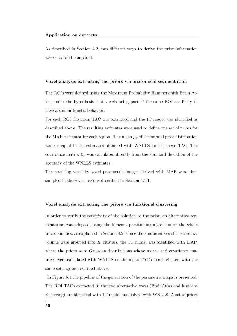
Application on datasets
As described in Section 4.2, two different ways to derive the prior information
were used and compared.
Voxel analysis extracting the priors via anatomical segmentation
The ROIs were defined using the Maximum Probability Hammersmith Brain At-
las, under the hypothesis that voxels being part of the same ROI are likely to
have a similar kinetic behavior.
For each ROI the mean TAC was extracted and the 1T model was identified as
described above. The resulting estimates were used to define one set of priors for
the MAP estimator for each region. The mean µp of the normal prior distribution
was set equal to the estimates obtained with WNLLS for the mean TAC. The
covariance matrix Σp was calculated directly from the standard deviation of the
accuracy of the WNLLS estimates.
The resulting voxel by voxel parametric images derived with MAP were then
sampled in the seven regions described in Section 4.1.1.
Voxel analysis extracting the priors via functional clustering
In order to verify the sensitivity of the solution to the prior, an alternative seg-
mentation was adopted, using the k-means partitioning algorithm on the whole
tracer kinetics, as explained in Section 4.2. Once the kinetic curves of the cerebral
volume were grouped into K clusters, the 1T model was identified with MAP,
where the priors were Gaussian distributions whose means and covariance ma-
trices were calculated with WNLLS on the mean TAC of each cluster, with the
same settings as described above.
In Figure 5.1 the pipeline of the generation of the parametric maps is presented.
The ROI TACs extracted in the two alternative ways (BrainAtlas and k-means
clustering) are identified with 1T model and solved with WNLLS. A set of priors
50
5.1 H-MAP on [11C]DPN
Figure 5.1: K1 and k2 parametric maps estimation pipeline. The dynamic PET images havebeen segmented using the anatomical Maximum Probability BrainAtlas or k-means clustering.The ROI TACs have been extracted and identified with the 1T model using WNLLS, obtainingthe priors for the two parameters. From the MAP estimation of the linearized 1T model theparametric maps for K1 and k2 were obtained.
for each region is determined. At voxel level, the 1T model is solved with a MAP
estimator, and the parametric maps for K1 and k2 are obtained. Finally, the
volume of distribution is calculated according to Eq. 2.19.
Assessment of the estimates
For parametric maps resulting from both types of priors, values of VT < 0 and
VT > 100 were not considered, because negative values of VThave no biological
explanation and values over 100 were clearly non-physiological, given the fact
that the higher values in literature do not overcome 46.8 ml/g ([45]). Thus the
upper bound was more than twice larger than the highest value reported in liter-
ature and for this reason the range was considered very large in such a way that
outliers do not to have any impact on the final results.
The results obtained at the voxel level with priors extracted from the atlas and
51

Application on datasets
the results obtained with priors extracted from functional clustering will be re-
ferred to as ’H-MAP A’ and ’H-MAP C’ respectively.
The H-MAP A estimates were compared with the results obtained at the ROI
level using both LEGA and the 1T model estimated with WNLLS on each ROI’s
TAC. More in detail, for each ROI the VT estimates obtained with H-MAP A
were averaged in the voxels composing the ROI area, and these average values
were compared to the ROI estimates.
The correlation among the results with a regression analysis was evaluated: the
slope and the intercept of the fitted regression line with ROI LEGA as indepen-
dent variable and the mean of H-MAP A in each ROI as dependent variable were
calculated for each subject. Pearson’s R2 values were reported as the correlation
measure.
For the assessment of the test-retest estimates, for each subject, slope and in-
tercept of the fitted regression line were calculated, with the mean of test and
retest H-MAP A estimates in each ROI as independent and dependent variable
respectively. Pearson’s R2 values were added as correlation measures.
To evaluate the H-MAP C results the effects that the change of the method for
extracting the priors has on the estimates were assessed, so the H-MAP C re-
sults were compared with the estimates obtained with H-MAP A and reported
as percentage, according to:
difference% =1
N
∑N
i=1
1P
∑Pj=1 V
i,jT,cluster −
1P
∑Pj=1 V
i,jT,atlas
1P
∑Pj=1 V
i,jT,atlas
∗ 100 (5.4)
where N is the number of subjects (considering test and retest together), P the
number of voxels of the ROI, V i,jT,cluster the value of the H-MAP C estimate in the
jth voxel for the ith subject and V i,jT,atlas the value of the H-MAP A estimate in the
jth voxel for the ith subject. An additional criterion to evaluate the performance
of H-MAP A and H-MAP C was the quantification of the coefficient of variation
52
5.2 H-BFM on [11C]WAY100635 and [11C]FLB457
of the parameters to assess their precision.
To further assess the reliability of the method the intraclass correlation coefficient
(ICC) for repeated test-retest PET studies was also calculated:
ICC =MS(bs)−MS(ws)
MS(bs) +MS(ws)(5.5)
where MS = mean sum of squares, bs = between subjects and ws = within sub-
jects.
For test-retest data acquired under similar conditions, true intrasubject differ-
ences will be small, so high ICCs will be expected ([84]). We calculated ICCs
using the ’one way random’ model reporting the ’single measure’ ICC.
5.2 H-BFM on [11C]WAY100635 and [11C]FLB457
H-BFM was tested on both [11C]FLB457 and [11C]WAY100635 datasets. For
these tracers the optimal model to describe the kinetic behavior in the brain was
the 2T model (Figure 2.1, of Eq. 2.1 and Eq. 2.2). The parameter of interest
was VT , calculated according to Eq. 2.3.
The data were affected by a measurement error, which was assumed to be addi-
tive, uncorrelated, from a Gaussian distribution with zero mean and covariance
matrix Σv, estimated as the square of the known standard deviation less than a
scale factor γ. The proportionality constant γ was estimated a posteriori as in
[39] and [40] according to Eq. 5.3. As no Bayesian estimator is employed, m = n
and nb = 0.
Basis Functions
As explained in Section 3.3, the 2T model was at first solved at the ROI level for
each region with WNLLS, using a Levenberg-Marquardt minimization procedure
53
Application on datasets
as implemented in Matlab.
The relative weights for the individual data points were defined as the inverse of
the variance of the decay-corrected activity, i.e. frame length over whole brain
activity, as in [82].
The local grids for the basis functions were generated automatically from the
data, from the estimates obtained at ROI level, according to Figure 3.2.
The exponent coefficients β1 and β2 of the two convolutions were evaluated from
the ROI individual rate constants as in Eq. 2.8 and from these values one grid
for each convolution of the measurement equation for each region was defined.
The grids were created 2-dimensional, based on a sampling of Gaussian distribu-
tions, whose means are the exponents estimated at ROI level and the standard
deviations are calculated directly from the precision of the estimates.
The size of the grids was chosen appropriately to limit the required computa-
tional time but also to give enough information for the voxel-wise analysis. The
size was set equal to 20x20.
Then starting from Eq. 2.7 for each time frame (i = 1, . . . , n, with n number
of frames), basis functions were pre-calculated for the non linear terms involving
Cp(t) according to Eq. 3.8, obtaining one set of B1l(t) and B2l(t), for each ele-
ment l = 1, . . . ,M of the grids β1 and β2 (as defined in Eq. 2.8).
Thus, Eq. 2.7 became:
CV OI = [B1l B2l Cb]
α1
α2
Vb
(5.6)
where CV OI is the vector of the measures with dimension nx1, Cb has dimension
nx1 and the parameters to be estimated are α1, α2 and Vb. B1l and B2l are
the nx1 basis functions for the two convolutions for the lth element of the grids,
54
5.2 H-BFM on [11C]WAY100635 and [11C]FLB457
defined as in Eq. 3.8 as:
Bjl(ti) = Cp(ti)⊗ e−βjlti l = 1, . . . ,M (5.7)
Eq. 5.6 was then solved with weighted linear least squares for each element of the
grids, choosing as best solution the one which minimizes the WRSS (Eq. 3.9), as
in [2] and the individual kinetic rate constants were calculated from the estimated
α1 and α2.
Voxel analysis extracting the priors via anatomical segmentation
The ROIs were defined using the Maximum Probability Brain Atlas and for each
ROI the mean TAC was extracted and the 2T model was identified as described
in the previous section. The resulting estimates were used to define two grids for
the basis functions for each region, based on the sampling of Gaussian distribu-
tions.
The mean was set equal to the estimates obtained with WNLLS for the mean
TAC. The covariance matrix was calculated directly from the standard deviation
of the accuracy of the WNLLS estimates.
The resulting voxel by voxel parametric images derived with H-BFM were then
sampled in the seven regions selected for [11C]FLB457 and [11C]WAY100635
dataset, as described in Section 4.1.2 and Section 4.1.3 respectively.
Voxel analysis extracting the priors via functional clustering
In order to investigate the impact of varying the grid specifications, an alterna-
tive cluster segmentation was implemented, applying the k-means partitioning
algorithm on the whole tracer kinetics of [11C]FLB457 dataset, as explained in
Section 4.2.
Instead, on [11C]WAY100635 dataset a more complex clustering algorithm based
55

Application on datasets
on the parametrization of the kinetics was implemented, as described in Section
4.2. The slope and the intercept of the regression line were evaluated on the last
5 points of the voxel TACs, corresponding to the last 40 minutes of the PET
exam. The threshold applied to the probability map obtained from the Fuzzy
C-means was set equal to 85%, an high value not too restrictive.
Once the kinetic curves of the cerebral volume were grouped into K clusters,
the 2T model was identified with H-BFM, where the grids were created from the
sampling of Gaussian distributions whose means and covariance matrices were
calculated with WNLLS on the mean TAC of each cluster, with the same set-
tings as described above.
Assessment of the estimates
For parametric maps resulting from both types of grids, for both datasets, val-
ues of VT < 0 were not considered, because negative values have no biological
explanation. Moreover a higher bound for VT was set, i.e. VTcutoff = 25 for
[11C]FLB457 and VTcutoff = 10 for [11C]WAY100635 , as values for the volume
of distribution higher than the cutoff are clearly non-physiological.
In fact for these tracers the maximum values of VT in literature are 16.2 ml/g
and 6.7 ml/g respectively ([56], [62]) and the bounds were 50% higher than these
values, resulting in a very large range in order for outliers to not have any impact
on the final results.
The results obtained at the voxel level with grids extracted from the atlas and the
results obtained with grids extracted from functional clustering will be referred
to as ’H-BFM A’ and ’H-BFM C’ respectively.
The H-BFM A estimates were compared with the results obtained at voxel level
using 2T model solved with WNLLS at voxel level. More in detail, for each ROI
the VT estimates obtained with H-BFM A in the voxels composing the ROI area
were averaged, and these average values were compared to the average of the VT
56

5.2 H-BFM on [11C]WAY100635 and [11C]FLB457
estimates obtained with WNLLS in the same voxels.
The correlation among the results was evaluated with a regression analysis: the
slope and the intercept of the fitted regression line with the mean of VT WNLLS
in each ROI as independent variable and the mean of H-BFM A in each ROI
as dependent variable were calculated for each subject. Pearson R2 values were
reported as the correlation measure.
To evaluate the H-BFM C results, the effect that the change of the methods cho-
sen to define the grids has on the estimates was quantified with Eq. 5.4, where
V i,jT,cluster is the value of the H-BFM C estimate in the jth voxel for the ith sub-
ject and V i,jT,atlas the value of the H-BFM A estimate in the jth voxel for the ith
subject.
Another criterion to evaluate the performance of H-BFM A and H-BFM C was
the coefficient of variation of the parameters to assess their precision.
57


Chapter 6
Results
6.1 H-MAP results
ROI analysis
In Figure 6.1 the scatterplot of VT values obtained at the ROI level with com-
partmental analysis (x axis) and LEGA at ROI level (y axis) is presented. All the
700 ROIs considered for the 10 studies (five test, five retest, subscribed ’a’ and
’b’ respectively) were included. The ventricles and some small structures giving
rise to noisy data were excluded (subcallosal area, nucleus accumbens, substantia
nigra). There was excellent agreement and strong correlation among the 1T and
LEGA estimates at ROI level (R2 = 0.96), as already found previously ([85]) and
the regression line was nearly a bisector even if it seems to detect some difference
at high VT values.
Voxel analysis - priors from atlas
Figure 6.2 shows the parametric maps of VT obtained with H-MAP A for a rep-
resentative subject (subject 3a), on the three planes (coronal, top left; sagittal,
top right; transverse, bottom image). The percentage of voxels out of the range
defined in Chapter 5 was less than 0.4% for this subject: < 0.21% of voxels esti-
59

Results
Figure 6.1: Scatterplot of ROI analysis VT values estimated using WNLLS (x axis) and LEGA(y axis), obtained for all 700 ROIs considered for the 10 studies (five test, five retest). The redline is the identity line. Pearson’s correlation coefficient R2 is reported and the value of slopeand intercept of the fitted regression line are presented.
Figure 6.2: Parametric map of VT obtained with H-MAP A for subject 3a, shown in the threeplanes: coronal (top left), sagittal (top right), and transverse (bottom image). A Gaussian filter(FWHM 1.18 mm) was used to smooth the images before visualization. Note the high signal inthe thalamus (top left and bottom image) and the intermediate signal of the frontal cortex (topright and bottom image).
60

6.1 H-MAP results
Figure 6.3: Scatterplot of VT values estimated using LEGA on ROI data (x axis) versus theaverage of all voxels in the ROIs, after correction for non physiological estimates of VT valuesestimated using H-MAP A (y axis) for subject 3. Black dots (o) correspond to test data (subject3a) and blue crosses (+) correspond to retest data (subject 3b). The red line is the identityline. Pearson’s correlation coefficient R2 are reported for each test and the value of slope andintercept of the fitted regression line are presented.
mates were negative, and < 0.18% of voxels had VT values above 100. In general
for all the subjects the percentage out of the range was always less than 1.4% for
VT < 0 and less than 1.2% for VT > 100.
The regional distribution of VT was consistent with known opioid receptor dis-
tribution ([49]). More specifically, it can be seen in Figure 6.2 that the thalamus
had the highest signal (top left and bottom images), followed by frontal cortex
(top right and bottom images). The cerebellum (not present in the images) and
the occipital cortex had the lowest signal.
In Figure 6.3 the scatterplot of VT values estimated using LEGA at the ROI level
(x axis) versus the average values of VT calculated from the H-MAP A parametric
map for each ROI (y axis) is presented for a representative subject (3a and 3b).
There was good agreement and strong correlation among the estimates (for this
subject global R2 > 0.97) and the regression line was nearly a bisector.
In Table 6.1 the values of the Pearson’s value and the estimated slope of the
fitted regression line are reported for each subject (test and retest). On average,
61

Results
correlation regression linecoefficient R2 (slope)
sub 1a 0.95 0.81sub 1b 0.94 0.76sub 2a 0.96 0.83sub 2b 0.96 0.81sub 3a 0.98 0.90sub 3b 0.98 0.89sub 4a 0.99 0.85sub 4b 0.97 0.77sub 5a 0.81 0.65sub 5b 0.94 0.85
mean 0.94 0.81SD % 5% 7%
Table 6.1: Summary statistics (Pearson’s value R2 and slope of the fitted regression line) forthe 10 studies (five subjects, one test and one retest data set each), subscribed ’a’ and ’b’respectively) for LEGA ROI versus H-MAP A VT (average of all voxels in the ROIs).
ROIVT ROI LEGA VT ROI WNLLS VT H-MAP A
[ml/g] 1T [ml/g] [ml/g]
Hippocampus 17.7 ± 3.7 17.0 ± 3.5 17.1 ± 3.0Cerebellum 15.2 ± 2.4 16.0 ± 3.1 15.1 ± 2.5Brainstem 11.2 ± 2.3 11.2 ± 2.4 12.4 ± 2.3
Inferior frontal gyrus 28.5 ± 5.1 28.8 ± 6.5 26.8 ± 4.6Thalamus 35.6 ± 7.2 35.7 ± 8.9 32.8 ± 6.0
Lingual gyrus 11.3 ± 7.2 11.4 ± 2.4 11.1 ± 1.7Putamen 41.6 ± 9.2 42.3 ± 10.5 38.6 ± 7.7
Table 6.2: Inter subject regional values of VT obtained from the parametric maps of H-MAPA (average of all voxels in the ROIs) are compared with the values of VT obtained from ROIanalysis (LEGA and WNLLS applied to the 1T compartmental model). The values are reportedas mean ± SD.
there was very strong correlation among the methods (R2 = 0.94), and just for
one subject (5a) R2 was < 0.9. In Table 6.2 the values of VT obtained with
H-MAP A are compared with the VT values estimated by ROI analysis. The
H-MAP A method provided good results, similar to the ROI methods, even if
there was a small underestimation of less than 3% of H-MAP A compared with
the ROI methods. The average estimate precision, expressed as between subject
SDs, improved, being on average 4.0 ml/g against 4.5 ml/g for ROI LEGA and
5.3 ml/g for ROI WNLLS.
62
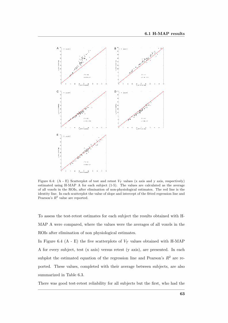
6.1 H-MAP results
Figure 6.4: (A - E) Scatterplot of test and retest VT values (x axis and y axis, respectively)estimated using H-MAP A for each subject (1-5). The values are calculated as the averageof all voxels in the ROIs, after elimination of non-physiological estimates. The red line is theidentity line. In each scatterplot the value of slope and intercept of the fitted regression line andPearson’s R2 value are reported.
To assess the test-retest estimates for each subject the results obtained with H-
MAP A were compared, where the values were the averages of all voxels in the
ROIs after elimination of non physiological estimates.
In Figure 6.4 (A - E) the five scatterplots of VT values obtained with H-MAP
A for every subject, test (x axis) versus retest (y axis), are presented. In each
subplot the estimated equation of the regression line and Pearson’s R2 are re-
ported. These values, completed with their average between subjects, are also
summarized in Table 6.3.
There was good test-retest reliability for all subjects but the first, who had the
63

Results
correlation regression linecoefficient R2 (slope)
sub 1 0.90 1.53sub 2 0.96 0.98sub 3 0.93 0.81sub 4 0.96 0.99sub 5 0.95 1.02
mean 0.94 1.07SD % 3% 27%
Table 6.3: Summary statistics (Pearson’s value R2 and slope of the fitted regression line) forthe estimates obtained with H-MAP A (average of all voxels in the ROIs) in test versus retestdata for the five subjects.
H-MAP A H-MAP C
sub 1a 0.51 0.56sub 1bsub 2a 0.93 0.94sub 2bsub 3a 0.91 0.92sub 3bsub 4a 0.93 0.92sub 4bsub 5a 0.97 0.96sub 5bmean 0.85 0.86SD % 22% 20%
Table 6.4: correlation coefficients (ICCs) are presented for VT values obtained with H-MAP Aand H-MAP C for all the subjects in the seven ROIs described in the text.
smallest Pearson’s value (R2 < 0.9), whereas for all other subjects R2 > 0.92
(average R2 > 0.93), and the regression line was similar to the bisector. Subject
1 also had the slope furthest from unity, and the largest intercept, among the
subjects.
For H-MAP A, the average ICC value among the subjects for each of the seven
ROIs was 0.85, and it was lowest (0.51) for the first subject, as expected (Table
4). ICCs between 0.82 and 0.96 have been rated as good or excellent ([86]).
64
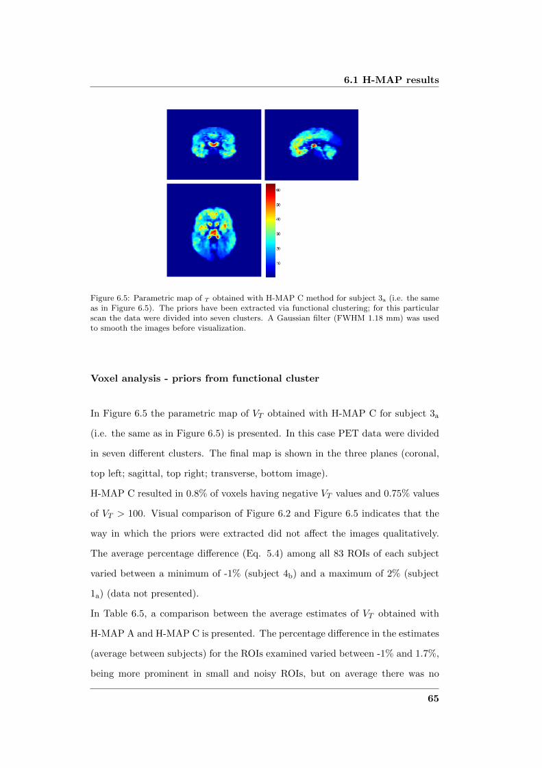
6.1 H-MAP results
Figure 6.5: Parametric map of T obtained with H-MAP C method for subject 3a (i.e. the sameas in Figure 6.5). The priors have been extracted via functional clustering; for this particularscan the data were divided into seven clusters. A Gaussian filter (FWHM 1.18 mm) was usedto smooth the images before visualization.
Voxel analysis - priors from functional cluster
In Figure 6.5 the parametric map of VT obtained with H-MAP C for subject 3a
(i.e. the same as in Figure 6.5) is presented. In this case PET data were divided
in seven different clusters. The final map is shown in the three planes (coronal,
top left; sagittal, top right; transverse, bottom image).
H-MAP C resulted in 0.8% of voxels having negative VT values and 0.75% values
of VT > 100. Visual comparison of Figure 6.2 and Figure 6.5 indicates that the
way in which the priors were extracted did not affect the images qualitatively.
The average percentage difference (Eq. 5.4) among all 83 ROIs of each subject
varied between a minimum of -1% (subject 4b) and a maximum of 2% (subject
1a) (data not presented).
In Table 6.5, a comparison between the average estimates of VT obtained with
H-MAP A and H-MAP C is presented. The percentage difference in the estimates
(average between subjects) for the ROIs examined varied between -1% and 1.7%,
being more prominent in small and noisy ROIs, but on average there was no
65

Results
ROIVT H-MAP A VT H-MAP C % difference
[ml/g] [ml/g]
Hippocampus 17.1 ± 3.0 16.9 ± 3.1 -1.0%Cerebellum 15.1 ± 2.5 15.3 ± 2.6 1.2%Brainstem 12.4 ± 2.3 12.6 ± 2.3 1.7%
Inferior frontal gyrus 27.2 ± 4.8 28.8 ± 6.5 1.6%Thalamus 32.8 ± 6.0 33.2 ± 5.8 1.1%
Lingual gyrus 11.1 ± 1.7 11.2 ± 1.7 0.4%Putamen 38.6 ± 7.7 38.8 ± 7.8 0.3%
Table 6.5: Regional values of VT (mean of all voxel in the ROIs) and their average percentagedifferences obtained from H-MAP C parametric maps compared with values of VT obtained withH-MAP A. The values are reported as inter-subjects mean ± SD.
difference among the two methods. The average estimate precision did not vary
either.
ICCs for H-MAP C estimates were also calculated as a measure of reliability. The
average ICC was excellent at 0.86, and it was again lowest for the first subject
(0.56) as in Table 6.4.
6.1.1 Discussion
The method was tested on a 1T model, but it can be applied to any linear or
linearized PET model. The priors for the Bayesian estimator are generated auto-
matically from the data, and as a consequence are user-independent, overcoming
the limitations of such methods as spectral analysis. Unlike methods like GLLS
or GTS, this method does not require any iteration, and the bias introduced by
the linearization of the model is resolved by the Bayesian estimation, so the crit-
ical choice of a termination criterion is avoided.
In comparison with the Bayesian method proposed in [7] also based on a Maxi-
mum a Posteriori estimator, this method differs in several fundamental aspects
such as here a linear MAP estimator is used instead of a more computational
expensive nonlinear estimator, the unknown scale factor of the variance matrix
of the measurement error is derived on the basis of the reproducible method de-
66
6.1 H-MAP results
scribed in [39] and in [40] and it does not require the use of additional images
besides the data of the subject under analysis to define the a priori information.
Differently from the Bayesian approach proposed in [7], H-MAP assumes a pop-
ulation composed by voxels, and relies on the hypothesis that the parameter es-
timates derived at ROI level (or by clustering) are representative of the expected
model parameter values of the voxels composing the ROI itself (or cluster). The
standard deviation of the parameter estimation error, derived from the inverse
of Fisher’s matrix, represents the between-voxels (i.e. between-subjects) possible
variability.
The method is robust, as it allows a reliable estimation of model parameters in
all but a few brain voxels. It is based on a linear optimization process, so it is not
time consuming and suitable to analyze large amounts of data, as for example in
voxel by voxel analyses.
The performance of the novel method for quantifying [11C]DPN data was as-
sessed. The H-MAP A and H-MAP C results had strong agreement with those
obtained by using both graphical analysis and compartmental model solved by
WNNLS, applied at the ROI level, and the identified regional distribution of
opioid receptors was consistent with those found in previous studies ([49]). The
reliability among test-retest estimates was also very good for all subjects but
one.
The high variability in test-retest results for subject 1 is to be attributed to
movement artifacts (see Figure 1 in [45]). The movement was substantial and it
is likely that it had not been completely eliminated during the movement correc-
tion step, affecting consequently the test - retest estimates.
In literature, [11C]DPN kinetics have mainly been described with a 2T model
([49], [43]), but it was difficult to obtain reliable estimates of k3/k4 values from
a single [11C]DPN tracer study.
67

Results
Therefore to understand whether this difficulty was due to over-parameterization,
both 1T and 2T models were applied to [11C]DPN dataset and compared at the
ROI and voxel level, solving them with WNLLS.
The performance of the models in fitting ROI TACs was assessed using the Akaike
Information Criterion (AIC); the precision of the estimates expressed as their
between-subject standard deviation and the percentage of model failures at the
voxel level. For further comparison also the values estimated via LEGA applied
to ROIs were used, as they are supposed to be unbiased.
Both at the ROI and voxel level, the 1T model best described the available
[11C]DPN dataset.
6.2 H-BFM results
[11C]FLB457
In Figure 6.6 the parametric maps of VT estimated with H-BFM A (Figure 6.6A)
and H-BFM C (Figure 6.6B) are presented for a representative subject (subject
3). For this subject the percentage of a out-physiological-range voxels (as de-
scribed in Section 5.2) was less than 2% for H-BFM A and less than 3% for
H-BFM C. In general for all the subjects for both methods the percentage out of
range was always less than 2% for VT < 0 and less than 6% for VT > 25 (taking
in account that around 1.5% of the voxels higher than the cutoff belongs to the
striatum which is not considered due to the too short scanning protocol).
Instead, WNLLS VT estimates out of range were in general > 30% (for this sub-
ject, more than 36% of voxels had VT > 25) being the non linear estimator more
sensitive to noise in the data.
The regional distribution of VT was consistent with known dopamine receptor
distribution ([54]). More specifically, it can be seen in Figure 6.6A and Fig-
ure 6.6B that the striatum had the highest radioactivity concentration. Beside
68

6.2 H-BFM results
Figure 6.6: (A-B) Parametric maps of [11C]FLB457 VT estimated with H-BFM A (A) and H-BFM C (B) of a representative subject (subject 3). Note the high signal in the striatum and inextrastriatal regions as thalamus, temporal and frontal cortices. (C) Scatterplot of the averagevalues of VT estimated using WNLLS at voxel level (x axis) versus the average values of VT
calculated from the H-BFM parametric map for each ROI (y axis) of the same subject (H-BFMA, blue diamonds, and H-BFM C, red squares). The black line is the identity line. Pearson’scorrelation coefficients R2 are reported for each test and the value of slope and intercept ofthe fitted regression line are presented. (D) Pearson’s values for each subject (H-BFM A andH-BFM C)
.
69

Results
the striatum, not considered due to the too short scanning protocol, conspicu-
ous radioactivity was found in extrastriatal regions as thalamus, temporal and
frontal cortices. The cerebellum (not present in the images) had the lowest signal.
In Figure 6.6C the scatterplot of the average values of VT estimated using WNLLS
at voxel level (x axis) versus the average values of VT calculated from the H-BFM
parametric map for each ROI (y axis) is presented for the same subject (H-BFM
A, blue diamonds, and H-BFM C, red squares). There was good agreement and
strong correlation among the estimates (for this subject R2 > 0.93 for H-BFM
A and R2 > 0.98) and the regression line was nearly a bisector. In Figure 6.6D
the values of the Pearson’s value are reported for each subject (H-BFM A and
H-BFM C). On average, there was very strong correlation among the methods
(in average R2 > 0.92 and R2 > 0.96 respectively).
In Figure 6.7A the values of VT obtained with H-BFM A and H-BFM C are
compared with the VT values estimated by voxel WNLLS analysis. In average
there was no difference in the estimates when the grids are defined based on
anatomical or functional segmentation.
The H-BFM methods provided good results, with no difference in the estimates
of H-BFM A and H-BFM C, which were similar to those obtained with the non
linear estimator, even if there was a small overestimation of less than 10% of H-
BFM compared with the WNLLS methods. As said, more than 30% of WNLLS
estimates are eliminated, while only < 8% of H-BFM results are out of range
(also taking in account striatum voxels), so H-BFM estimates were compared
only in the voxels with reliable WNLLS values of VT . In this case, as expected,
there is still no difference in the results of H-BFM C compared to H-BFM A, and
the difference previously reported between H-BFM results compared to WNLLS
estimates lowers to less than 1%.
70

6.2 H-BFM results
Figure 6.7: Inter subject regional values of VT obtained with H-BFM A and H-BFM C arecompared with the VT values estimated by voxel WNLLS analysis for [11C]FLB457 data (A)and for [11C]WAY100635 data (B). The average estimate precision is expressed as betweensubject SDs. Hipp = hippocampus, Amy = amygdala, Cer = cerebellum, Tha = thalamus,Front Ctx = frontal cortex, Temp Ctx = temporal cortex, Ant Cing = anterior cingulate.
71

Results
Figure 6.8: (A-B). Parametric maps of [11C]WAY100635 VT estimated with H-BFM A (A) andH-BFM C (B) of a representative subject (subject 4). Note the high signal in the insula followedby frontal and temporal cortices and anterior cingulate. (C) Scatterplot of the average valuesof VT estimated using WNLLS at voxel level (x axis) versus the average values of VT calculatedfrom the H-BFM parametric map for each ROI (y axis) of the same subject (H-BFM A, bluediamonds, and H-BFM C, red squares). The black line is the identity line. Pearson’s correlationcoefficients R2 are reported for each test and the value of slope and intercept of the fittedregression line are presented. (D) Pearson’s values for each subject (H-BFM A and H-BFM C).
[11C]WAY100635
In Figure 6.8 the parametric maps of VT estimated with H-BFM A (Fig 6.8A)
and H-BFM C (Fig 6.8B) are presented for a representative subject (subject 4).
For this subject the percentage of voxels of out physiological range was less than
1% for both H-BFM A and H-BFM C.
In general for both methods the percentage out of range was always less than 2%
for VT < 0 and less than 1% for VT > 25. Instead, WNLLS VT estimates out
of range were in general > 30% (for this subject, more than 32% of voxels had
72
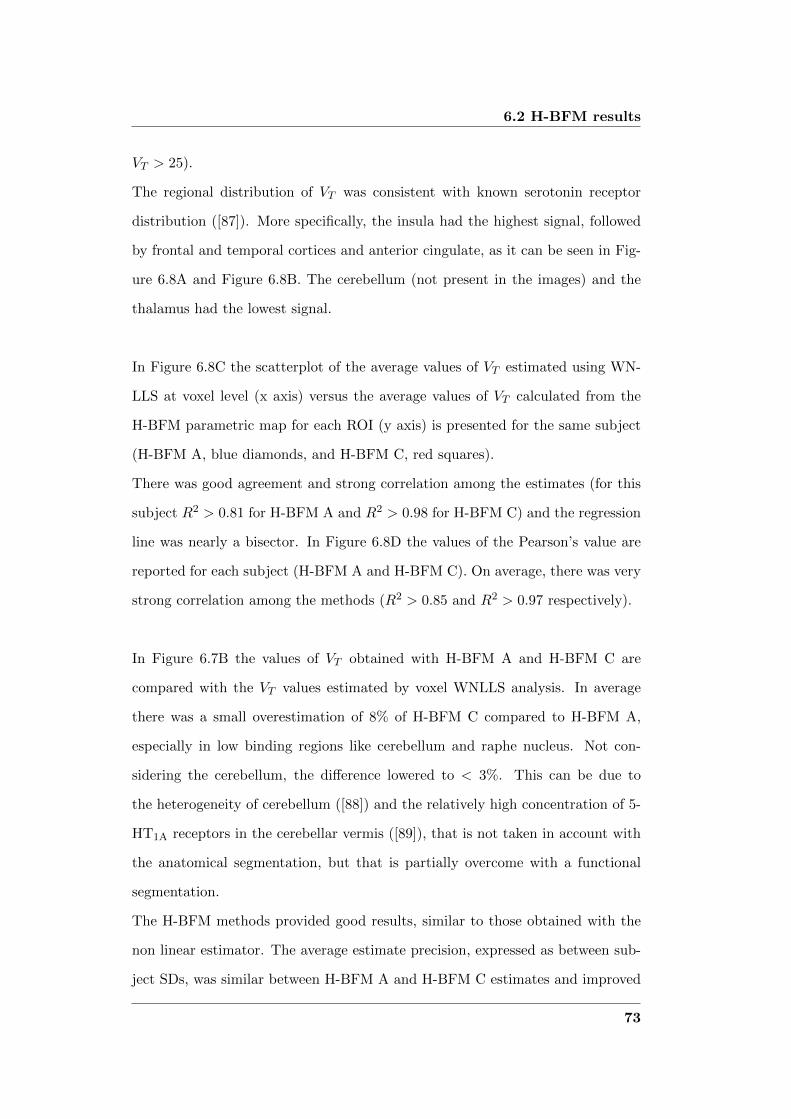
6.2 H-BFM results
VT > 25).
The regional distribution of VT was consistent with known serotonin receptor
distribution ([87]). More specifically, the insula had the highest signal, followed
by frontal and temporal cortices and anterior cingulate, as it can be seen in Fig-
ure 6.8A and Figure 6.8B. The cerebellum (not present in the images) and the
thalamus had the lowest signal.
In Figure 6.8C the scatterplot of the average values of VT estimated using WN-
LLS at voxel level (x axis) versus the average values of VT calculated from the
H-BFM parametric map for each ROI (y axis) is presented for the same subject
(H-BFM A, blue diamonds, and H-BFM C, red squares).
There was good agreement and strong correlation among the estimates (for this
subject R2 > 0.81 for H-BFM A and R2 > 0.98 for H-BFM C) and the regression
line was nearly a bisector. In Figure 6.8D the values of the Pearson’s value are
reported for each subject (H-BFM A and H-BFM C). On average, there was very
strong correlation among the methods (R2 > 0.85 and R2 > 0.97 respectively).
In Figure 6.7B the values of VT obtained with H-BFM A and H-BFM C are
compared with the VT values estimated by voxel WNLLS analysis. In average
there was a small overestimation of 8% of H-BFM C compared to H-BFM A,
especially in low binding regions like cerebellum and raphe nucleus. Not con-
sidering the cerebellum, the difference lowered to < 3%. This can be due to
the heterogeneity of cerebellum ([88]) and the relatively high concentration of 5-
HT1A receptors in the cerebellar vermis ([89]), that is not taken in account with
the anatomical segmentation, but that is partially overcome with a functional
segmentation.
The H-BFM methods provided good results, similar to those obtained with the
non linear estimator. The average estimate precision, expressed as between sub-
ject SDs, was similar between H-BFM A and H-BFM C estimates and improved
73

Results
especially in high binding regions using H-BFM C, being on average 0.71 ml/g
against 0.63 ml/g for H-BFM A.
6.2.1 Discussion
The performance of the novel method for quantifying [11C]FLB457 and [11C]WAY
100635 data was assessed. The H-BFM A and H-BFM C results had strong agree-
ment with those obtained by using compartmental model solved by WNNLS, ap-
plied at the voxel level, and the identified regional distribution of receptors was
consistent with those found in previous studies ([54], [87]).
In average, the difference in the estimates between WNLLS and H-BFM was
less than 1% (once considering H-BFM estimates only in the voxels with reliable
WNLLS values of VT ).
H-BFM is robust and faster than WNLLS (at least three times faster) and its
application on both [11C]FLB457 457 and [11C]WAY100635 allows accurate quan-
tification of VT and good quality parametric maps.
H-BFM allows user-independent PET quantification, where the grids are defined
automatically from the data, subject and ROI specific. To the author’s knowl-
edge there are only two previous works which developed the BFM for multi-
compartmental models ([3] and [4]), but in that approach the grids were global
and user-defined.
In particular, in [3] the grids were 2-dimensional, each dimension constituted by
100 logarithmically spaced element. The ranges were defined, fixed for all voxels
regardless of the anatomical region, from values presented in literature.
Grids defined in such a way imply the linear estimation process to be repeated
10’000 times for each voxel, resulting in a very demanding computational analy-
sis.
In [3] and in [4], BFMs were also applied to a 3K model, with 1-dimensional grid
74
6.3 Results based on functional clustering
with 100 basis function. Having only one convolution to be solved, the grid can
be dense with no particular effect on the required computational time. Neverthe-
less the grids were defined logarithmically and fixed for all cerebral voxels and all
subjects.
6.3 Results based on functional clustering
K-means on whole kinetics: [11C]DPN and [11C]FLB457
For both datasets, the partitioning method of choice was the k-means, applied to
the whole tracer kinetics, as described in Chapter 5.
The optimal number of clusters, K, was automatically selected as the greatest
possible number which keeps the centroids statistically different between each
other. The statistical difference was tested with the Wilcoxon’s test, as imple-
mented in Matlab.
For [11C]DPN data, for all subjects but one, six or seven clusters were enough
to describe all significantly different kinetics within the brain. For subject 1a
and 1b, the optimal number of clusters was eight and nine for the test and retest
scans, respectively.
In this case the way to derive the priors does not affect the final results: the
images did not differ qualitatively, and the average percentage difference of esti-
mates was less than 1% (Table 6.5).
The different segmentations had no impact on [11C]FLB457 final estimates, as no
differences in the results were detected, as can be seen in Figure 6.7. Note that
for both tracers, in the final masks, even if the clusters were created grouping the
TACs on the base only of their kinetics, it was easy to verify also good agreement
with anatomical segmentation, as can be seen in Figure (6.9).
75
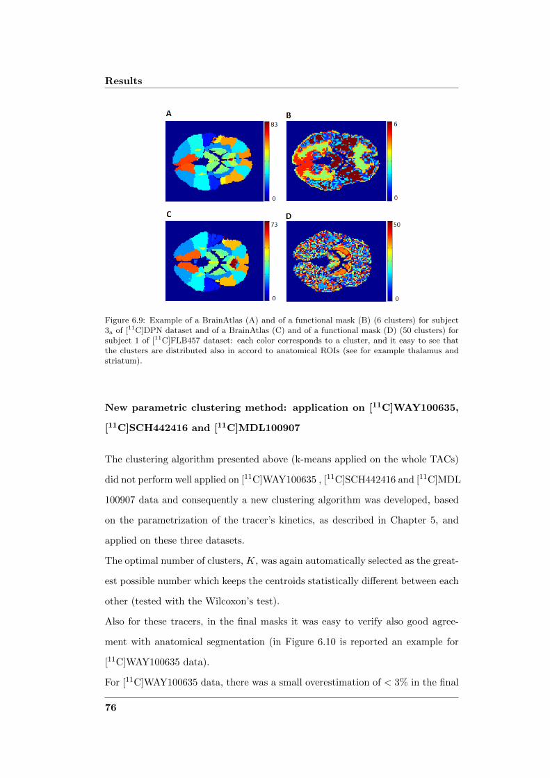
Results
Figure 6.9: Example of a BrainAtlas (A) and of a functional mask (B) (6 clusters) for subject3a of [11C]DPN dataset and of a BrainAtlas (C) and of a functional mask (D) (50 clusters) forsubject 1 of [11C]FLB457 dataset: each color corresponds to a cluster, and it easy to see thatthe clusters are distributed also in accord to anatomical ROIs (see for example thalamus andstriatum).
New parametric clustering method: application on [11C]WAY100635,
[11C]SCH442416 and [11C]MDL100907
The clustering algorithm presented above (k-means applied on the whole TACs)
did not perform well applied on [11C]WAY100635 , [11C]SCH442416 and [11C]MDL
100907 data and consequently a new clustering algorithm was developed, based
on the parametrization of the tracer’s kinetics, as described in Chapter 5, and
applied on these three datasets.
The optimal number of clusters, K, was again automatically selected as the great-
est possible number which keeps the centroids statistically different between each
other (tested with the Wilcoxon’s test).
Also for these tracers, in the final masks it was easy to verify also good agree-
ment with anatomical segmentation (in Figure 6.10 is reported an example for
[11C]WAY100635 data).
For [11C]WAY100635 data, there was a small overestimation of < 3% in the final
76
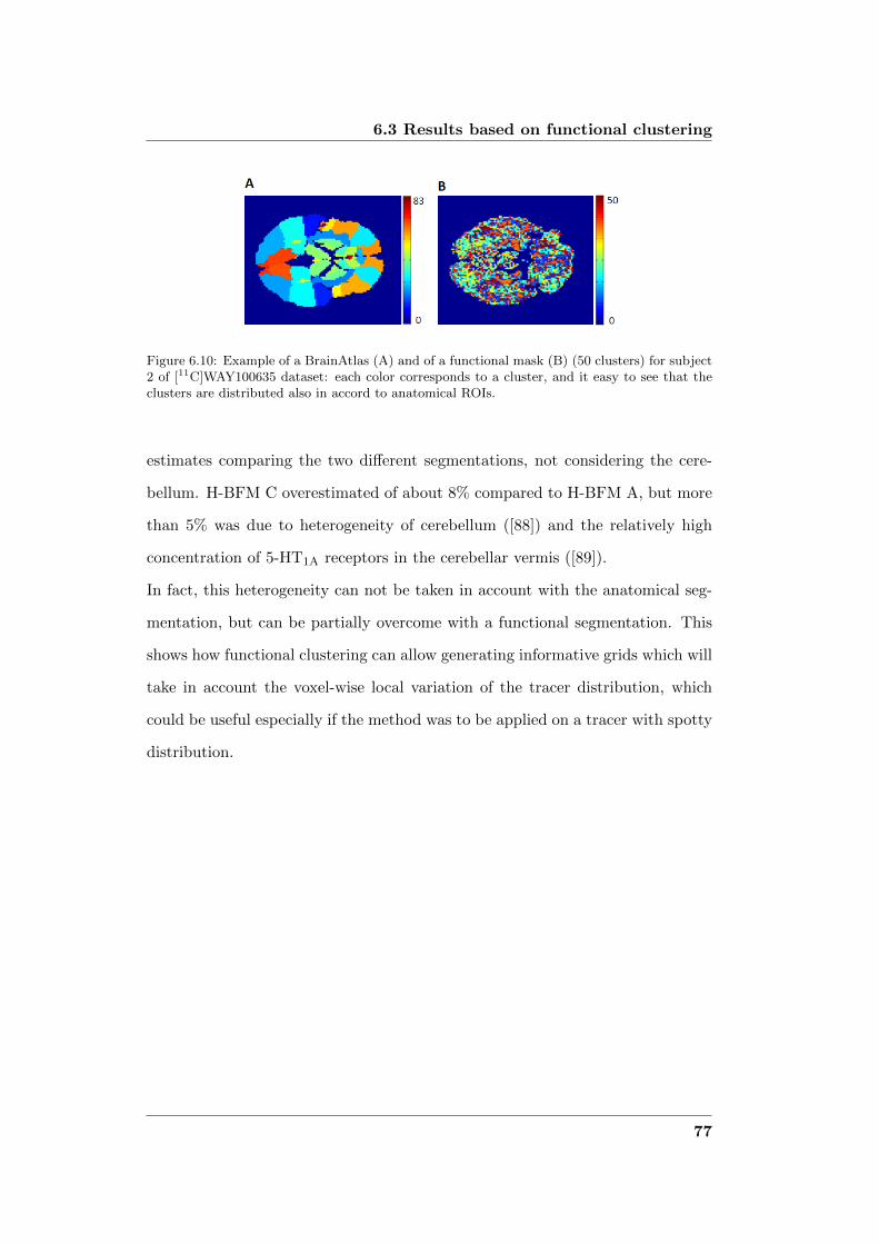
6.3 Results based on functional clustering
Figure 6.10: Example of a BrainAtlas (A) and of a functional mask (B) (50 clusters) for subject2 of [11C]WAY100635 dataset: each color corresponds to a cluster, and it easy to see that theclusters are distributed also in accord to anatomical ROIs.
estimates comparing the two different segmentations, not considering the cere-
bellum. H-BFM C overestimated of about 8% compared to H-BFM A, but more
than 5% was due to heterogeneity of cerebellum ([88]) and the relatively high
concentration of 5-HT1A receptors in the cerebellar vermis ([89]).
In fact, this heterogeneity can not be taken in account with the anatomical seg-
mentation, but can be partially overcome with a functional segmentation. This
shows how functional clustering can allow generating informative grids which will
take in account the voxel-wise local variation of the tracer distribution, which
could be useful especially if the method was to be applied on a tracer with spotty
distribution.
77


Chapter 7
Additional work: development
of novel compartmental models
for quantification of PET
tracer kinetics
As described previously, both novel methods H-MAP and H-BFM are model-
driven methods, based on compartmental models. When the optimal model
to be used to describe the data was not already presented in literature it has
been necessary to develop the compartmental model to quantify the tracer under
study using model- and data-driven methods. In particular, new compartmen-
tal models for [11C]SCH442416 and for [11C]MDL100907 data were developed.
[11C]SCH442416 data have never been quantified with compartmental models in
humans before and for [11C]MDL100907 the model presented in literature was
not appropriate for the fit of the available data.
79

Additional work: development of novel compartmental models forquantification of PET tracer kinetics
Figure 7.1: Dynamic PET images summed over the first 2 min, shown in the three plane(transverse, coronal, sagittal), of subject 1 (A) and subject 5 (B). For both subjects the vascularcomponent is clearly detectable.
7.1 Modeling [11C]SCH442416 dataset
As described in Section 4.1.4, quantitative assessment of A2A receptor expres-
sion from [11C]SCH442416 PET images in human brain have been made by using
spectral analysis ([67] and [68]) revealing the presence of both reversible and ir-
reversible components.
The aim of this study is to develop the compartmental model to quantify [11]SCH
442416 kinetics at voxel level in healthy control subjects, based on the results pre-
sented in [69], using the dataset described in Section 4.1.4.
In order to develop the model, a preliminary analysis on the tissue and plasma
data was carried out. [11C]SCH442416 showed an important vascular component
in all subjects, especially for two subjects. As it can be seen from the dynamic
PET summed over the first 2 min (in Figure 7.1), for both subjects (subject 1,
80

7.1 Modeling [11C]SCH442416 dataset
Figure 7.2: Two tissue-three rate constants in parallel (3K-parallel) compartmental model. K1
(ml/g/min) and k2 (min-1) represent first order rate constants for transport of ligand fromplasma to tissue (C1) and vice versa. Kb (ml/g/min) is the rate constant from plasma to thetrapping vascular component (C2).
A, and subject 5, B) a notable vascular component was clearly detectable. This
vascular component made it very difficult to generate the atlas and to properly
estimate the model parameters. Moreover, a clear asymmetry in the vascular
contribute was recognized.
A preliminary assessment on the model structure was carried out.
7.1.1 Model structure
Two tissue-three rate constants compartmental model in parallel (3K-
parallel)
In Figure 7.2 the two tissue-three rate constants in parallel (3K-parallel) com-
partmental model proposed by [69] is presented. The tissue (C1) is represented
by one compartment for the non displaceable component (nd) plus a specifically
81

Additional work: development of novel compartmental models forquantification of PET tracer kinetics
bound fraction (sp), according to:
C1(t) = K1Cp(t)− k2C2(t) C1(0) = 0
C2(t) = KbCp(t) C2(0) = 0(7.1)
CV OI(t) = (1− Vb)C1(t) + Vb (C2(t) + Cb(t)) (7.2)
where K1 (ml/g/min) and k2 (min-1) represent first order rate constants for
transport of ligand from plasma to tissue and vice versa. Kb (ml/g/min) is the
rate constant from plasma to the trapping vascular component C2.
The parameter of interest is the total volume of distribution (VT , ml/g), which
is calculated from the ratio of the two tissue parameters as in Eq. 2.19.
As already described in Chapter 2, the model was solved with basis functions
obtaining the following equation:
CV OI(t) = (1− Vb)K1Cp(t)⊗ e−k2t + VbK1
∫ t
0Cp(τ)dτ + VbCb(t) (7.3)
The model was solved with H-BFM, as in Chapter 3, where the local grid for
the parameter k2 was defined for each region from the ROI estimates, solving the
model above with WNLLS. The grid was still created based on a sampling of a
Gaussian distribution, whose mean was the parameter k2 estimated at ROI level
and the standard deviation was calculated directly from the estimate precision.
As there was only one convolution to be solved, the grid was 1-dimensional and
the size was set equal to 100.
Three tissue-four rate constants compartmental model in parallel with
two input functions (4K-2IF)
The initial model presented in [69] was not appropriate to describe the data of
two subjects of the dataset (subject 1 and subject 5). An alternative model was
82
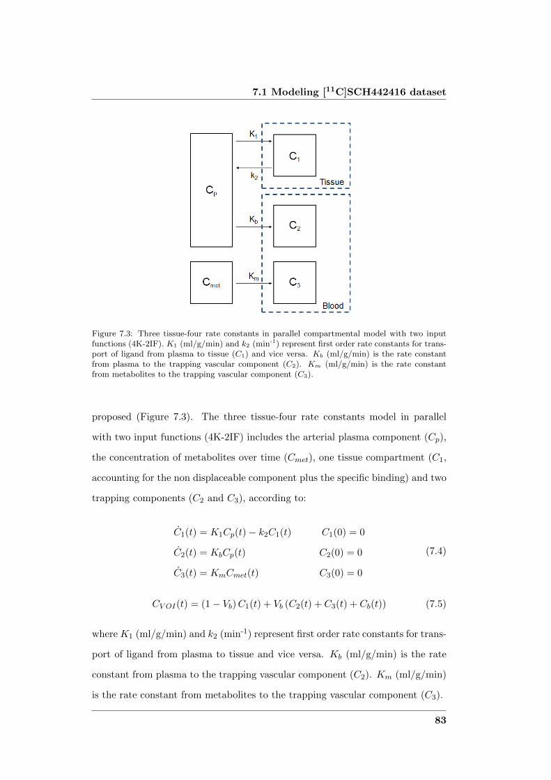
7.1 Modeling [11C]SCH442416 dataset
Figure 7.3: Three tissue-four rate constants in parallel compartmental model with two inputfunctions (4K-2IF). K1 (ml/g/min) and k2 (min-1) represent first order rate constants for trans-port of ligand from plasma to tissue (C1) and vice versa. Kb (ml/g/min) is the rate constantfrom plasma to the trapping vascular component (C2). Km (ml/g/min) is the rate constantfrom metabolites to the trapping vascular component (C3).
proposed (Figure 7.3). The three tissue-four rate constants model in parallel
with two input functions (4K-2IF) includes the arterial plasma component (Cp),
the concentration of metabolites over time (Cmet), one tissue compartment (C1,
accounting for the non displaceable component plus the specific binding) and two
trapping components (C2 and C3), according to:
C1(t) = K1Cp(t)− k2C1(t) C1(0) = 0
C2(t) = KbCp(t) C2(0) = 0
C3(t) = KmCmet(t) C3(0) = 0
(7.4)
CV OI(t) = (1− Vb)C1(t) + Vb (C2(t) + C3(t) + Cb(t)) (7.5)
where K1 (ml/g/min) and k2 (min-1) represent first order rate constants for trans-
port of ligand from plasma to tissue and vice versa. Kb (ml/g/min) is the rate
constant from plasma to the trapping vascular component (C2). Km (ml/g/min)
is the rate constant from metabolites to the trapping vascular component (C3).
83
Additional work: development of novel compartmental models forquantification of PET tracer kinetics
The parameter of interest is the total volume of distribution (VT , ml/g), which
is calculated from the ratio of the two tissue parameters as in Eq. 2.19.
As already described in Chapter 2, the model was solved with basis functions
obtaining the following equation:
CV OI(t) = (1− Vb)K1Cp(t)⊗ e−k2t + VbKb
∫ t
0Cp(τ)dτ+
+ VbKm
∫ t
0Cmet(τ)dτ + VbCb(t)
(7.6)
The model was solved with H-BFM, as in Chapter 3, where the local grid for the
parameter k2 was defined as above for model 3K-parallel.
The best model was chosen on the basis of a priori identifiability, a posteri-
ori numerical identifiability, and Akaike criterion. Goodness of the fit, estimates
included in the physiological interval and precision estimates were also evaluated.
7.1.2 4K-2IF model results
ROI analysis
At ROI level, for two subjects the optimal model to describe [11C]SCH442416 ki-
netics was the 4K-2IF one, while for the remaining 4 subjects the optimal model
was 3K-parallel. In particular, the presence of the second trapping component,
linked to the concentration of metabolites over time, was fundamental to obtain
a proper fit of the late part of the ROI curve for subject 1 and subject 5. In
Figure 7.4 is reported an example of fit of 3K-parallel (dashed lines) and 4K-2IF
model (dot dashed lines) to the tissue TAC of cerebellum (circles) for subject 1,
where it can be seen as 3K-parallel model is insufficient to properly describe the
data.
Instead 4K-2IF did not perform well applied to the other 4 subjects of the
84

7.1 Modeling [11C]SCH442416 dataset
Figure 7.4: Example of fit of 3K-parallel (dashed lines) and 4K-2IF model (dot dashed lines) tothe tissue TAC of cerebellum (circles) for subject 1.
datasets, as Km always tended to 0, resulting in 3K-parallel to be the best model.
Voxel analysis
For subject 1 and 5, 4K-2IF model failed at voxel level, VT was estimated negative
(i.e. not physiological) for more than 25% of the voxels, although the parametric
maps were quite uniform. In presence of higher level of noise (typical of the voxel-
wise analysis), the second vascular component was difficult to detect, and it was
often not estimated. Moreover, the model estimates suffered of the difficulties
due to the heavy vascular component, as shown in Figure 7.1. The same difficul-
ties will be found also for the simpler model. When a voxel was mainly vascular,
k2 tended to be very high, meaning that the tracer did not enter the tissue, and
consequently the exchange between Cp and C1 was too fast to be detected and
the structure collapsed.
Various attempts to separate the tissue and vascular information were made. At
85
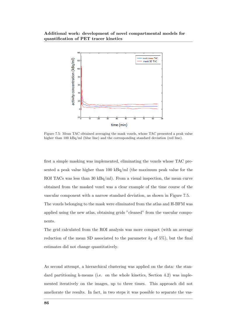
Additional work: development of novel compartmental models forquantification of PET tracer kinetics
Figure 7.5: Mean TAC obtained averaging the mask voxels, whose TAC presented a peak valuehigher than 100 kBq/ml (blue line) and the corresponding standard deviation (red line).
first a simple masking was implemented, eliminating the voxels whose TAC pre-
sented a peak value higher than 100 kBq/ml (the maximum peak value for the
ROI TACs was less than 30 kBq/ml). From a visual inspection, the mean curve
obtained from the masked voxel was a clear example of the time course of the
vascular component with a narrow standard deviation, as shown in Figure 7.5.
The voxels belonging to the mask were eliminated from the atlas and H-BFM was
applied using the new atlas, obtaining grids ”cleaned” from the vascular compo-
nents.
The grid calculated from the ROI analysis was more compact (with an average
reduction of the mean SD associated to the parameter k2 of 5%), but the final
estimates did not change quantitatively.
As second attempt, a hierarchical clustering was applied on the data: the stan-
dard partitioning k-means (i.e. on the whole kinetics, Section 4.2) was imple-
mented iteratively on the images, up to three times. This approach did not
ameliorate the results. In fact, in two steps it was possible to separate the vas-
86

7.1 Modeling [11C]SCH442416 dataset
Figure 7.6: Inter subject regional values of VT obtained with H-BFM A and H-BFM C arecompared with the VT values estimated by voxel WNLLS analysis for [11C]SCH442416 data.The average estimate precision is expressed as between subject SDs.
cular information from the tissue, obtaining a mask similar to the one obtained
with the previous attempt, but once extracted the tissue information, it was no
possible to properly segment the image. The cluster analysis only managed to
segment the white matter from the gray matter, with no use for an appropriate
brain segmentation.
H-BFM was applied anyway using the clustered regions, and the same observa-
tions made for the results obtained with anatomical segmentation held: when
a voxel contained mainly vascular information, k2 was very high and the model
collapsed.
7.1.3 3K-parallel model results
The model of choice to describe [11C]SCH442416 data is 3K-parallel, as already
found in [69].
The 3K-parallel model was applied to all subjects and solved with H-BFM as
described above.
In Figure 7.6 the values of VT obtained with H-BFM A and H-BFM C are com-
87

Additional work: development of novel compartmental models forquantification of PET tracer kinetics
pared with the VT values estimated by voxel WNLLS analysis. In average there is
almost no difference in the estimates when the grids are defined based on anatom-
ical or functional segmentation (difference% was less than 1%).
The H-BFM methods provided good results, with no difference in the estimates
of H-BFM A and H-BFM C, which were similar to those obtained with the non
linear estimator, with only a small overestimation of less than 3% of H-BFM
compared with the WNLLS methods.
VT estimates showed a large variability, considering for example the striatum, in
which VT ranged from a value of 0.09 ml/g (subject 1) up to 0.57 ml/g (subject
3). The lower VT estimates were found for subject 1 and subject 5 (in stria-
tum VT = 0.11 ml/g), as expected, being the subjects with the higher vascular
component. As already noted, the presence of a vascular contribute led to high
estimates of Kb (for these subjects in average values higher than 150% compared
to the other subjects) and especially of k2 (values in average higher than 200%
compared to the other subjects), resulting in very low estimates of VT .
In Figure 7.7 the parametric maps of VT estimated with H-BFM A (Fig. 7.7A)
and H-BFM C (Fig.7.7B) are presented for a representative subject (subject
3). Less than 10% of voxels had VT < 0 and less of 1% of voxel presented
VT > VTcutoff = 1.
The regional distribution of VT reflected the known physiological distribution of
adenosine receptor ([63], [68]).
In Figure 7.7C the scatterplot of the average values of VT estimated using WNLLS
at voxel level (x axis) versus the average values of VT calculated from the H-BFM
parametric map for each ROI (y axis) is presented for the same subject (H-BFM
A, blue diamonds, and H-BFM C, red squares). There was good agreement and
strong correlation among the estimates (for this subject R2 > 0.85 for H-BFM
A and R2 > 0.90) and the regression line was nearly a bisector. In Figure 7.7D
the values of the Pearson’s value are reported for each subject (H-BFM A and
88

7.1 Modeling [11C]SCH442416 dataset
Figure 7.7: (A-B) Parametric maps of [11C]SCH442416 VT estimated with H-BFM A (A) andH-BFM C (B) for a representative subject (subject 3). (C) Scatterplot of the average values ofVT estimated using WNLLS at voxel level (x axis) versus the average values of VT calculatedfrom the H-BFM parametric map for each ROI (y axis) of the same subject (H-BFM A, bluediamonds, and H-BFM C, red squares). The black line is the identity line. Pearson’s correlationcoefficients R2 are reported for each test and the value of slope and intercept of the fittedregression line are presented. (D) Pearson’s values for each subject (H-BFM A and H-BFM C)
.
89
Additional work: development of novel compartmental models forquantification of PET tracer kinetics
H-BFM C). On average, there was very strong correlation among the methods
(in average R2 > 0.78 and R2 > 0.85 respectively).
In general, H-BFM C showed a better correlation with WNLLS results compared
to H-BFM A. This effect was expected because of the high heterogeneity due to
the notable vascular component present in all subjects, which could not be taken
in account with the anatomical segmentation, but was partially overcome with a
functional segmentation.
The same attempt already made for 4K-2IF model to reduce the vascular con-
tribute with functional hierarchical clustering was applied to subject 4. The
cluster identifying the vascular component was eliminated from the anatomical
atlas and H-BFM A was applied on the new atlas.
The ROI estimates did not change, but the correlation with WNLLS results im-
proved (R2 > 0.9), confirming the vascular correction to be a promising approach
for [11C]SCH442416 estimation at voxel level with H-BFM.
7.1.4 Discussion
4K-2IF model gave good results at ROI level for 2 subjects out of 6 (probably
due to heterogeneity). The additional component was necessary for a proper fit
of the tail of the region TACs, but for [11C]SCH442416 data the best model to
be applied on voxel level was a three compartmental one.
An analysis on tissue and input data for subject 1 and 5 was carried out. A
possible explanation for the necessity of a different model to properly fit the data
could be related to difference in metabolism. In fact from a comparison of Cmet(t)
it resulted that the concentration of the metabolites increased in the late part of
the PET exam, i.e. the value of the slope of the curve evaluated from 20 min to
the end of the scan was positive, in contrast with the values for the other subjects
which were negative.
90
7.1 Modeling [11C]SCH442416 dataset
The possibility that the two components detected with spectral analysis ([67],
[68], [69]) could refer to a 3K model in series (as in Figure 2.2, Eq. 2.9, Eq. 2.10)
was discussed. In this case the trapping component could be due to binding to
receptors or production of metabolites in the tissue.
From physiological data, adenosine A2A receptors are known to be abundant in
basal ganglia, vasculature and platelets. Consequently VT is expected to be high
in striatum, pallidum and nucleus accumbens.
If k3 is related to receptor binding, the macroparameter K is expected to be high
in rich receptor density ROIs (same ROIs with high VT ).
If k3 is related to production of metabolites in the tissue, VT should be related
to receptor density.
When applied to [11C]SCH442416 data, the 3K model presented physiological
estimates of Vb (Vb ∼ 0.05) and VT estimates well correlated with known recep-
tor distribution but much higher than spectral analysis values (up to ten times
higher). Also the exchange between the plasma and non displaceable compart-
ment resulted higher than expected.
Moreover, in rich receptor density ROIs high VT values were detected, but a low
K was estimated, indicating that the trapping was not related to binding to re-
ceptors.
Instead, 3K-parallel model provided physiological values of Vb (Vb ∼ 0.05) and
the estimated VT was well correlated with the known receptor density and com-
parable to spectral analysis results.
In 3K-parallel model, Kb represents the trapping to the vascular component and
it is expected to be correlated to receptor density in vascular system. Previous
studies showed that A2A receptors are expressed in the vessels and platelets ([90],
[91]), confirming the model interpretation, but it should be elaborated on how to
justify this physiological interpretation.
91
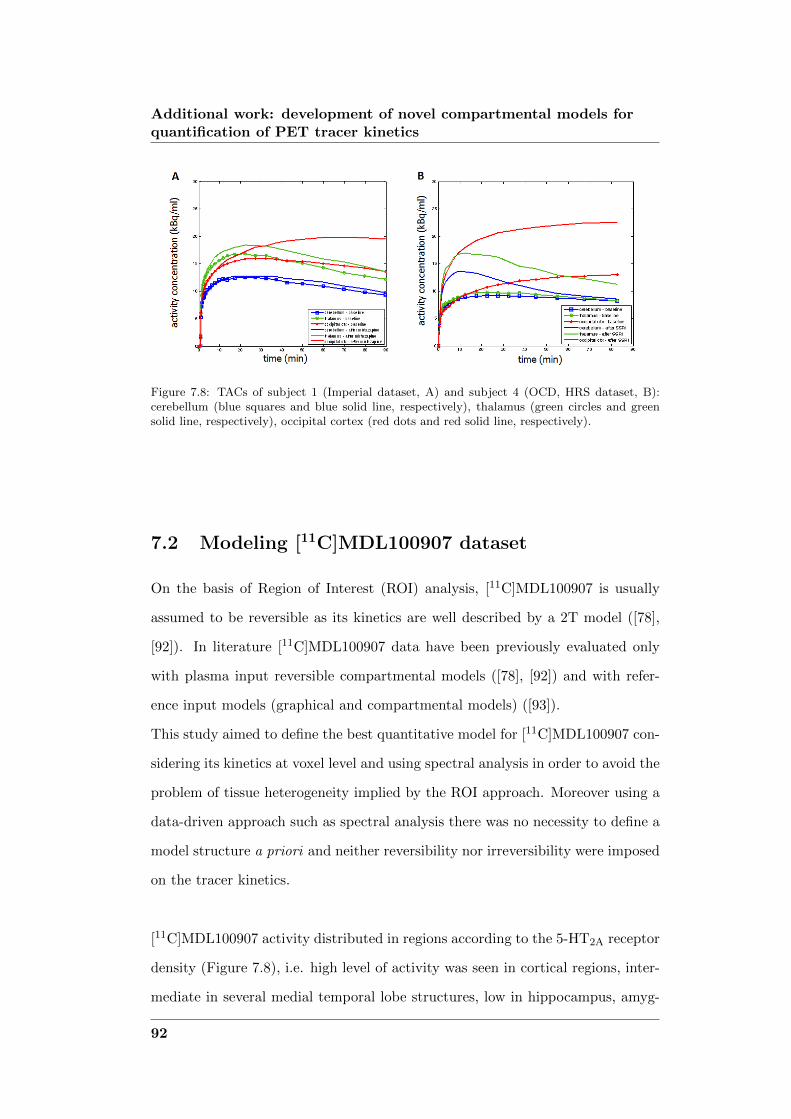
Additional work: development of novel compartmental models forquantification of PET tracer kinetics
Figure 7.8: TACs of subject 1 (Imperial dataset, A) and subject 4 (OCD, HRS dataset, B):cerebellum (blue squares and blue solid line, respectively), thalamus (green circles and greensolid line, respectively), occipital cortex (red dots and red solid line, respectively).
7.2 Modeling [11C]MDL100907 dataset
On the basis of Region of Interest (ROI) analysis, [11C]MDL100907 is usually
assumed to be reversible as its kinetics are well described by a 2T model ([78],
[92]). In literature [11C]MDL100907 data have been previously evaluated only
with plasma input reversible compartmental models ([78], [92]) and with refer-
ence input models (graphical and compartmental models) ([93]).
This study aimed to define the best quantitative model for [11C]MDL100907 con-
sidering its kinetics at voxel level and using spectral analysis in order to avoid the
problem of tissue heterogeneity implied by the ROI approach. Moreover using a
data-driven approach such as spectral analysis there was no necessity to define a
model structure a priori and neither reversibility nor irreversibility were imposed
on the tracer kinetics.
[11C]MDL100907 activity distributed in regions according to the 5-HT2A receptor
density (Figure 7.8), i.e. high level of activity was seen in cortical regions, inter-
mediate in several medial temporal lobe structures, low in hippocampus, amyg-
92

7.2 Modeling [11C]MDL100907 dataset
dale, and lowest in thalamus and cerebellum. At baseline, for both datasets, in
cerebellum, thalamus and hippocampus, activity peaked relatively early (12-22
min), while in medial temporal lobe structures it peaked later (27-45 min). In
neocortical regions, peak activity was reached slowly (55-90 min).
For Imperial dataset, there was a clear qualitative difference in the tracer activity
in neocortical regions at baseline and blocked condition for each subject (Figure
7.8), while no relative changes were observed in cerebellum and thalamus kinet-
ics.
In HSR dataset, no changes were detected in neocortical regions after adminis-
tration of SSRI (Figure 7.8), while it was possible detect a change in the kinetics
of low binding regions (cerebellum and thalamus).
7.2.1 Metabolite curve fitting
Both Imperial data and HSR dataset included plasma measures not corrected for
metabolites.
Various models are available in literature for the fit of the unmetabolized parent
fraction of [11C]MDL100907 ([72] and [78]). The model reported in [78] refines
the previous model of [72], which was derived empirically. The novel model
contains an additional parameter q3 which reflects the proportion of radioactivity
in plasma at time zero, which is not due to parent compound. Positive values
of this parameter could represent radiochemical impurities or rapidly formed
radiolabelled metabolites in the body, and probably it is related to the rapid
metabolism of [11C]MDL100907 as it is the parameter with the greatest inter-
and intra-subject variability.
This model was appropriate for the fit of the unmetabolized parent radiotracer
measures of both Imperial and HSR dataset. The model is described by:
Ppf(t) =(1 + (q1t)
2)−q2 − q3 with q1 > 0, q2 > 0, q3 > 0 (7.7)
93
Additional work: development of novel compartmental models forquantification of PET tracer kinetics
where Ppf(t) is the parent plasma fraction. The model was solved with WN-
LLS, using a Levenberg-Marquardt minimization procedure as implemented in
Matlab. The relative weights for the individual data points were defined as the
inverse of the variance associated to the data, up to a scale factor γ, where the
variance was modeled assuming Poisson statistics. The proportionality constant
γ was estimated a posteriori as in [39] and [40].
For the subjects without any metabolites data (HSR dataset) the estimates ob-
tained from the fit of the average of all measures were used for the description of
the unmetabolized parent fraction.
After the generation of the individual PPf , for each sampling time ti (i =
1, . . . , n, with n total number of frames) the parent plasma input function (Cp)
was obtained for each subject by multiplying the Ppf with the measures of tracer
concentration in plasma uncorrected for metabolites (Cmeas) as in:
Cp(ti) = Cmeas(ti) · Ppf(ti) (7.8)
Finally, the concentration of the radioactivity in the whole blood (Cb) was calcu-
lated as:
Cb(ti) = (1− 0.3 ·H)Cmeas(ti) (7.9)
where H is the hematocrit, set by default at 0.8 ([94]).
7.2.2 Classic Spectral Analysis (SA)
Spectral analysis (SA) utilizes a general input-output model to identify the ki-
netic components of tissue tracer activity without any specific compartmental
model assumptions ([5], [95]). The system output is described by the convolution
of the input function with an exponential impulse response that has real-valued,
decaying exponents. Once the spectrum of kinetic components has been esti-
94
7.2 Modeling [11C]MDL100907 dataset
mated, knowledge of the tracer’s biochemical and/or physiololgical properties
can be used to relate parameters of the identified spectrum to measures of the
process of interest.
In spectral analysis, the concentration of radioactivity in tissue at time t, CT (t),
is modeled as a convolution of the plasma time-activity curve, Cp(t), with the
sum of M+2 distinct exponential terms as:
CT (t) =∑M+1
j=0Cp(t)⊗ αje−βjt =
∑M+1
j=0αj
∫ t
0Cp(τ)e−βj(t−τ)dτ (7.10)
where αj and βj are assumed to be real-valued and nonnegative. In Eq. 7.10 the
maximum number of terms to be included in the model, M +2, is predefined and
set to an arbitrary large number, e.g., 100.
Possible values of βj are fixed to cover a biological plausible spectral range, and
values of αj are estimated from blood and tissue TACs by a nonnegative least
squares procedure. In practice, only a few components with αj > 0 are detected
([96]). The factors determining which components are identified are the definition
of the grid, the measurement error affecting the data, the sensitivity of the ra-
dioactivity to the changes in the intervals of the exponents, the algorithm chosen
and the convergence criteria ([95]).
From Eq. 7.10 it can be observed that ”high-frequency” components, i.e., com-
ponents with very large βj , become proportional to Cp(t), accounting for the
fast passage of the tracer in the vascular space of the ROI (vascular volume or
spillover component, Vb), whereas ”low-frequency” components, i.e., those with
βj = 0 or near zero, become proportional to∫Cp(t)dt and account for trapping
of tracer. Components with intermediate values of βj reflect tissue compartments
within the ROI that exchange material directly or indirectly with plasma, giving
an indication of tissue heterogeneity.
It must be recalled that the spectra components do not depend on a specific
model and the interpretation of the parameters of the different components can
95
Additional work: development of novel compartmental models forquantification of PET tracer kinetics
be derived only on the basis of a structural model. However from the estimated
parameters is possible to derive the total binding rate constant (K, ml/g/min)
for irreversible tracers, or the total volume of distribution (VT , ml/g).
Eq. 7.10 can be written to explicitly show the trapping of tracer and the vascular
component Vb as:
CT (t) = α0
∫ t
0Cp(τ)dτ+
∑M
j=1αj
∫ t
0Cp(τ)e−βj(t−τ)dτ + VbCb(t) (7.11)
The SA in its original version presents some problems, first of all the so called
”line doubling”. As the βj ’s values of the grid are discrete, often the true spec-
tra components fall between two consecutive values and the algorithm cannot
always place a component in the exact position that would yield the best fit of
the data: in this case the respective βj are estimated with low precision ([39]).
Also, the method requires the βj to be positive. Among the most common prob-
lems, there is also the identification of very slow components (”phantom”), which
are not present in the original data. The shorter the scanning schedule and the
higher the noise level, the broader the distribution of phantom components ([95]).
In general, a lower cutoff frequency, βcutoff , is defined and all the components
in the tissue with 0 < βj < βcutoff are considered resulting from noise in the
data, shifting trapping components from their true position in βj = 0, while
components with βj > βcutoff are assumed to correspond to real equilibrating
process in the system. This value of cutoff is generally calculated as in [95], i.e.
βcutoff = 1/Tend, where Tend is the end time of the scan.
7.2.3 Non Linear Spectral Analysis (NLSA)
A new SA method (Non Linear Spectral Analysis, NLSA) was proposed in [39]
by revisiting the classic SA as an exponential impulse response identification
problem and overcoming the issues described in the previous section (the non
96
7.2 Modeling [11C]MDL100907 dataset
negativity constraint for αj , the low precision of the estimates, the line doubling
and the impossibility to convert the estimated parameters in kinetic variables).
In this revised approach, it is not necessary to define a grid for the eigenvalues
and to estimate the corresponding amplitudes, but the impulsive response func-
tion is identified by estimating the number of exponentials necessary to fit the
data solving models of increasing order using WNLLS. Then model parsimony
criteria as Akaike Information Criterion (AIC) are used to choose the best model.
It is to be noted that no constraints are required for αj and βj : in fact, even if the
impulsive response of a generic compartmental model must be always positive,
its coefficient do not have to be positive, unless input and output are in the same
compartment.
In the current study, six different models of increasing complexity were com-
pared, from a model with the only trapping component up to a model with three
reversible components, with the following equations:
CT (t) = (1− Vb)(α0
∫ t
0Cp(τ) dτ
)+ VbCb(t) (7.12)
CT (t) = (1− Vb)(α1
∫ t
0Cp(τ) e−β1(t−τ)dτ
)+ VbCb(t) (7.13)
CT (t) = (1− Vb)(α0
∫ t
0Cp(τ) dτ + α1
∫ t
0Cp(τ) e−β1(t−τ)dτ
)+ VbCb(t) (7.14)
CT (t) = (1− Vb)(α1
∫ t
0Cp(τ) e−β1(t−τ)dτ + α2
∫ t
0Cp(τ) e−β2(t−τ)dτ
)+ VbCb(t)
(7.15)
CT (t) = (1− Vb)(α0
∫ t
0Cp(τ) dτ + α1
∫ t
0Cp(τ) e−β1(t−τ)dτ+
+ α2
∫ t
0Cp(τ) e−β2(t−τ)dτ
)+ VbCb(t)
(7.16)
CT (t) = (1− Vb)(α1
∫ t
0Cp(τ) e−β1(t−τ)dτ + α2
∫ t
0Cp(τ) e−β2(t−τ)dτ+
+ α3
∫ t
0Cp(τ) e−β3(t−τ)dτ
)+ VbCb(t)
(7.17)
97
Additional work: development of novel compartmental models forquantification of PET tracer kinetics
where Vb, αj and βj were estimated with WNLLS, and the choice of the optimal
model to describe the data was based on AIC, goodness of the fit, estimates in-
cluded in the physiological interval and precision estimates.
It is to be noted that in this approach it is possible to obtain also the precisions
of βj , and not only of αj , and the problem of line doubling is clearly avoided.
Thus this approach provides model-independent information allowing selecting
the compartmental model appropriate for the description of the data.
7.2.4 NLSA results: ROI analysis
At ROI level, NLSA was implemented in order to avoid the problems related to
the classical version, given the low number of TACs to be analyzed and the higher
signal-to-noise ratio of the ROI curves.
The models selected for the implementation of the NLSA were described by Eq.
7.12 - 7.17, and the parameters were estimated at ROI level with a WNLLS
estimator, using a Levenberg-Marquardt minimization procedure as implemented
in Matlab. The relative weights were defined as the inverse of the variance of the
decay-corrected activity, i.e. frame length over TAC activity, less than a scale
factor γ, as defined in [39] and [40].
The value of cutoff was calculated as βcutoff = 1/Tend = 0.011 ([95]).
Results In Table 7.1 and Table 7.2 the results of the NLSA applied on ROI
are reported for Imperial and HSR datasets respectively. For both datasets, in
all subjects the majority of the regions were described by the model of Eq. 7.14,
i.e. one reversible and one irreversible component. Estimated parameters values
of α0, α1 and β1 and their precisions are reported.
As regard the Imperial dataset, for all subjects but one all the ROIs were best
described by the model of Eq. 7.14. For one subject, the amygdale, the frontal
cortex and the arterial cingulate were described by a model with only one re-
98

7.2 Modeling [11C]MDL100907 dataset
ROIVb α1 β1 α0
[unitless] [ml/g/min] [min−1] [ml/g/min]
Hippocampus 0.055 ± 0.028 0.280 ± 0.053 0.027 ± 0.011 0.134 ± 0.049Amygdalaa 0.062 ± 0.022 0.238 ± 0.048 0.022 ± 0.006 0.134 ± 0.049
Cerebellum 0.051 ± 0.034 0.319 ± 0.070 0.032 ± 0.002 0.067 ± 0.021Thalamus 0.061 ± 0.037 0.420 ± 0.056 0.028 ± 0.004 0.076 ± 0.026
Frontal cortexa 0.051 ± 0.034 0.278 ± 0.044 0.019 ± 0.004 0.169 ± 0.032Temporal cortex 0.047 ± 0.027 0.229 ± 0.056 0.019 ± 0.003 0.158 ± 0.031
Anterior cingulate 0.074 ± 0.043 0.328 ± 0.073 0.018 ± 0.003 0.199 ± 0.039Posterior lobea 0.049 ± 0.030 0.250 ± 0.047 0.020 ± 0.004 0.180 ± 0.036Occipital lobe 0.046 ± 0.028 0.281 ± 0.065 0.017 ± 0.004 0.159 ± 0.057
a Values are mean ± SD for 5 subjects.
Table 7.1: Inter-subject regional estimated parameters values of α0, α1 and β1 obtained fromROI analysis with NLSA (Imperial dataset). The values are reported as mean ± SD for 6subjects, except where indicated.
ROIVb α1 β1 α0
[unitless] [ml/g/min] [min−1] [ml/g/min]
Hippocampus 0.055 ± 0.011 0.206 ± 0.036 0.028 ± 0.003 0.181 ± 0.041Amygdala 0.060 ± 0.021 0.181 ± 0.055 0.034 ± 0.011 0.215 ± 0.048
Cerebellum 0.046 ± 0.003 0.279 ± 0.042 0.035 ± 0.006 0.177 ± 0.043Thalamus 0.056 ± 0.011 0.307 ± 0.032 0.029 ± 0.006 0.150 ± 0.041
Frontal cortexa 0.040 ± 0.006 0.212 ± 0.183 0.030 ± 0.006 0.291 ± 0.019Temporal cortexa 0.046 ± 0.002 0.185 ± 0.130 0.035 ± 0.005 0.296 ± 0.015
Anterior cingulatea 0.064 ± 0.006 0.190 ± 0.126 0.036 ± 0.021 0.354 ± 0.048Posterior lobea 0.045 ± 0.001 0.121 ± 0.004 0.030 ± 0.006 0.295 ± 0.019Occipital lobea 0.044 ± 0.004 0.144 ± 0.007 0.026 ± 0.005 0.314 ± 0.005
a Values are mean ± SD for 3 subjects.
Table 7.2: Inter-subject regional estimated parameters values of α0, α1 and β1 obtained fromROI analysis with NLSA (HSR dataset). The values are reported as mean ± SD for 4 subjects,except where indicated.
99

Additional work: development of novel compartmental models forquantification of PET tracer kinetics
versible component, but the estimated β1 < βcutoff , becoming compatible with
the irreversibility found in the other regions.
The irreversible component was especially detected in cortical regions with the
ratio α0/α1 ranging from 0.6 to 0.75, while in cerebellum and thalamus this ratio
was around 0.2, but the trapping was still clearly identified. The results con-
firmed what already presented in previous studies, i.e. tracer binding was high
in cortical regions, intermediate in temporal regions, low in hippocampus, amyg-
dale, and lowest in thalamus and cerebellum ([73], [78], [92]).
The fact that in some regions the results did not show the trapping line may
be due to a too short observation interval. In this interval the steady state was
not reached, and the model was consequently not definite yet, as the estimates
obtained for the reversible component model were not physiological.
The same held also for the HSR dataset. For all subjects but one, all ROIs were
best described by the model of Eq. 7.14, with one reversible and one irreversible
component. For one subject, the frontal and temporal cortex, the arterial cin-
gulate, the posterior and occipital lobe were described by a model with only one
reversible component, but the estimated β1 < βcutoff , becoming compatible with
the irreversibility found in the other regions. As for the Imperial dataset, the
irreversible component was especially detected in cortical regions with the ratio
α0/α1 ranging from 1.4 to 2.4, while in cerebellum and thalamus this ratio was
around 0.5, but the trapping was still clearly identified.
7.2.5 SA results: voxel analysis
As the TACs derived from a single voxel are characterized by a low signal-to-noise
ratio, and given the high number of TACs to be analyzed, the use of nonlinear
estimators can be difficult and unwieldy because of their computational cost.
Consequently, at voxel level the classical version of SA was implemented.
100

7.2 Modeling [11C]MDL100907 dataset
The grid for the βj ’s was defined as a logarithmic distribution of βj , j = 1, 2, . . . ,M
([97], [95]), with M + 1 set equal to 100. The lower limit of the distribution was
defined as β1 = 1/(3Tend) where Tend is the end time of the scan, and the up-
per limit was βM = (3/Tin) where Tin is the duration of the first scan ([95]).
Therefore the spacing of the βj ’s was fixed as:
βj =1
Tjand Tj = Tj−1
[TendTin
] 1M−1
for j = 2, 3, ...,M (7.18)
The M+1 unknown values αj were estimated with the weighted nonnegative
linear least squares algorithm implemented in Matlab by the lsqnonneg function.
The relative weights for the individual data points were defined as the inverse of
the variance of the decay-corrected activity, i.e. frame length over whole brain
activity. The whole brain activity was used instead of the activity in the voxel
due to the high noise of the voxel TACs. The value for the cutoff frequency was
βcutoff = 1/Tend as in [95].
Results SA results clearly showed at voxel level the presence of an irreversible
component, especially in cortical regions, thus confirming the results obtained at
ROI level with NLSA.
In Figure 7.9 the parametric map of the amplitude of irreversible component
K estimated with SA is presented for two representative subjects (subject 1 of
Imperial dataset, A, and subject 3 of HSR dataset, B). For both datasets, the
irreversible component was identified in more than 70% of the voxel.
In Table 7.3 the inter-subject average values (of all voxels in the 9 selected ROIs)
of K estimated with SA on the Imperial and HSR datasets are presented. The
values are reported as mean ± SD. Both from Figure 7.9 and Table 7.3 it can
be seen that the regional distribution of K was consistent with the known sero-
tonin receptor distribution ([73], [78], [92]). More specifically, in both datasets,
the cortical regions had the highest signal (the anterior cingulate, followed by
101
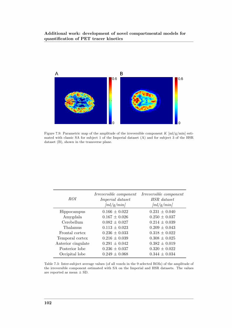
Additional work: development of novel compartmental models forquantification of PET tracer kinetics
Figure 7.9: Parametric map of the amplitude of the irreversible component K [ml/g/min] esti-mated with classic SA for subject 1 of the Imperial dataset (A) and for subject 3 of the HSRdataset (B), shown in the transverse plane.
ROIIrreversible component Irreversible component
Imperial dataset HSR dataset[ml/g/min] [ml/g/min]
Hippocampus 0.166 ± 0.022 0.231 ± 0.040Amygdala 0.167 ± 0.026 0.250 ± 0.037
Cerebellum 0.082 ± 0.027 0.214 ± 0.039Thalamus 0.113 ± 0.023 0.209 ± 0.043
Frontal cortex 0.236 ± 0.033 0.318 ± 0.022Temporal cortex 0.216 ± 0.039 0.308 ± 0.025
Anterior cingulate 0.291 ± 0.042 0.382 ± 0.019Posterior lobe 0.236 ± 0.037 0.320 ± 0.022Occipital lobe 0.249 ± 0.068 0.344 ± 0.034
Table 7.3: Inter-subject average values (of all voxels in the 9 selected ROIs) of the amplitude ofthe irreversible component estimated with SA on the Imperial and HSR datasets. The valuesare reported as mean ± SD.
102

7.2 Modeling [11C]MDL100907 dataset
posterior lobe and frontal cortex), while thalamus and cerebellum (not present
in the images) had the lowest signal. Only in cerebellar and thalamus voxels it
was possible to properly identify also a very slow reversible component, probably
due to the lack or reduced density of 5-HT2A.
In Figure 7.10 the weighted frequency spectrum, normalized to the peak consider-
ing all subjects of the datasets, is presented (Imperial, A, and HSR, B), with the
cerebellum (upper panel, red), thalamus (middle panel, black), temporal cortex
(lower panel, blue). The temporal cortex is a good representative of the other
cortical regions. As previously reported, in both cerebellum and thalamus it was
possible to clearly identify a reversible component almost as important as the
irreversible one (Figure 7.10, upper and middle panel), while for the cortex the
reversible component was generally lower and less frequent (Figure 7.10, lower
panel).
7.2.6 Discussion
Irreversibility of [11C]MDL100907 kinetic
Both at ROI and voxel level, an irreversible component was found in both dataset,
especially in cortical regions. At ROI level, only for one subject in each dataset,
some regions were described by a model with only one reversible component, but
the estimated β1 < βcutoff , becoming consistent with the irreversibility found in
the other regions. The fact that in some regions the results did not show the
trapping line may be due to a too short observation interval. In this interval the
steady state was not reached, and the model was consequently not definite yet,
as the estimates obtained for the one exponential model were not physiological.
At voxel level, the irreversible component was identified in more than 70% of the
voxel, especially in cortical regions, with a distribution consistent with the known
serotonin receptor distribution ([73], [78]), thus confirming the results obtained
103
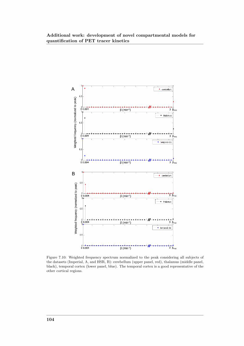
Additional work: development of novel compartmental models forquantification of PET tracer kinetics
Figure 7.10: Weighted frequency spectrum normalized to the peak considering all subjects ofthe datasets (Imperial, A, and HSR, B): cerebellum (upper panel, red), thalamus (middle panel,black), temporal cortex (lower panel, blue). The temporal cortex is a good representative of theother cortical regions.
104
7.2 Modeling [11C]MDL100907 dataset
at ROI level with NLSA. Only in cerebellar and thalamus voxels it was possible
to properly identify also a very slow reversible component, probably due to the
lack or reduced density of 5-HT2A.
In order to confirm the results obtained at voxel level with the classic SA, NLSA
was also implemented at voxel level for two subjects of both datasets, with the
same models (Eq. 7.12 - 7.17) and the same settings as for the estimation at ROI
level. The results confirmed those obtained with linear SA, the majority of the
voxel TACs were best described by the model of Eq. 7.12 i.e. one irreversible
component, (70% of voxels) while the remaining voxel TACs were best fitted by
the model of Eq. 7.14, i.e. one reversible and one irreversible component.
These results are in agreement with those found with the classic SA, as in high
binding regions only a small number of voxels had a second component, while in
low binding regions (cerebellum and thalamus), the second component was very
slow, but detectable.
As future work, an iterative filtered version of classical SA (Spectral Analysis
with Iterative Filter, [98]) will be applied to [11C]MDL100907 data in order to
overcome the problems of the original SA detailed above and to improve the ac-
curacy and the precision of the estimated spectrum.
The iterative filtered version has not been applied from the beginning to [11C]MDL
100907 data, as it works only on irreversible tracers and the presence of a trap-
ping component in [11C]MDL100907 kinetics was not proved yet.
A recent work ([92]) confirmed what already found previously in [78], particularly
the reversibility of the [11C]MDL100907 kinetics. It must be firstly highlighted
that this study is the first one to quantify [11C]MDL100907 data with a data-
driven model, i.e. not defining any a priori model structure neither imposing
reversibility or irreversibility of the tracer. It must be noted in this sense that all
previous studies had always quantified [11C]MDL100907 data only with reversible
105
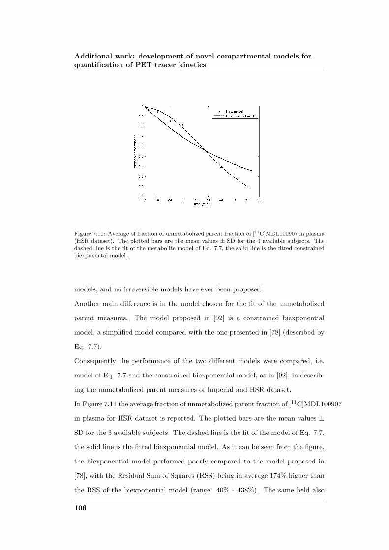
Additional work: development of novel compartmental models forquantification of PET tracer kinetics
Figure 7.11: Average of fraction of unmetabolized parent fraction of [11C]MDL100907 in plasma(HSR dataset). The plotted bars are the mean values ± SD for the 3 available subjects. Thedashed line is the fit of the metabolite model of Eq. 7.7, the solid line is the fitted constrainedbiexponental model.
models, and no irreversible models have ever been proposed.
Another main difference is in the model chosen for the fit of the unmetabolized
parent measures. The model proposed in [92] is a constrained biexponential
model, a simplified model compared with the one presented in [78] (described by
Eq. 7.7).
Consequently the performance of the two different models were compared, i.e.
model of Eq. 7.7 and the constrained biexponential model, as in [92], in describ-
ing the unmetabolized parent measures of Imperial and HSR dataset.
In Figure 7.11 the average fraction of unmetabolized parent fraction of [11C]MDL100907
in plasma for HSR dataset is reported. The plotted bars are the mean values ±
SD for the 3 available subjects. The dashed line is the fit of the model of Eq. 7.7,
the solid line is the fitted biexponential model. As it can be seen from the figure,
the biexponential model performed poorly compared to the model proposed in
[78], with the Residual Sum of Squares (RSS) being in average 174% higher than
the RSS of the biexponential model (range: 40% - 438%). The same held also
106
7.2 Modeling [11C]MDL100907 dataset
for Imperial dataset.
Having defined the optimal model for the fit of the unmetabolized measures, in
order to assess the impact of a different model on the final estimates, NLSA was
applied at ROI level using as forcing function the one obtained with the con-
strained biexponential model.
The optimal model for the majority of the region was the model of Eq. 7.15,
i.e. two reversible components, using as choice criteria only AIC. But once we
considered also goodness of fit and particularly the precision of estimates, the
optimal model was again the one of Eq. 7.14, i.e. one reversible and one irre-
versible component. The estimated precision of the microparameters obtained
for the more complex model was higher than 200%.
Moreover, considering each compartment estimated kinetics, it was easy to see
that the second reversible component constituted a ”fake” compartment, i.e. a
compartment whose kinetic has rate constant values close to zero.
Consequently, the choice of the model for the fit of the unmetabolized measures
is crucial, as it has a substantial impact on the quantification process.
Effect due to mirtazapine
After administration of blockade, there was a clear effect on cortical regions, while
low binding regions as thalamus and cerebellum were less affected.
Considering the plasma input function measured on the only one subject after
administration of mirtazapine (subject 1b), it was not possible to observe any
change in the arterial input function either.
NLSA was applied at voxel level on subject 1b, and the results obtained were in
agreement with those obtained on the other subjects analyzed at baseline, i.e.
65% voxel TACs were fitted with the model of Eq. 7.12 (one irreversible com-
ponent) and the remaining voxel TACs were best described by the model of Eq.
107
Additional work: development of novel compartmental models forquantification of PET tracer kinetics
7.14 (one reversible and one irreversible component).
On the basis also of previously published studies, the NLSA results could be in-
terpreted as respectively a 1tissue-1 rate constant (1K) model and a 3K model.
Once defined the model structure, it was possible to convert the spectral analysis
parameters into compartmental model ones.
The model parameters (described in Section 2.2, and indicating with K1 also the
rate constant for transport of tracer from plasma to tissue for model 1K) were
then compared between baseline and blocking studies, considering all voxel with-
out anatomical discrimination.
For the voxels where 1K was the optimal model, a reduction of 54% was found in
the value of K1 from baseline to blocking study (baseline: 0.414 ± 0.21; blocked:
0.191 ± 0.192). In the remaining voxels fitted with the 3K model, a reduction
of 49% was observed still on the K1 (baseline: 0.71 ± 0.217; blocked: 0.363 ±
0.287), while k2 and k3 remained almost unaltered in the two studies (k2: base-
line: 0.0351 ± 0.0386; blocked: 0.0372 ± 0.052; k3: baseline 0.0214 ± 0.021;
blocked: 0.0211 ± 0.023).
Consequently the blockade seemed to act on the input of the tracer in the tissue,
while the trapping was not affected. This resulted in a reduction on the value
of K1 for the 1K model, as in the simplified model the parameter contains infor-
mation of both the reversible and the irreversible components. Clearly, these are
the results of only one subject, and the analysis is not exhaustive, but it can be
considered as a general indication of the process.
From a short simulation (data not presented), the possibility that the difference
in K1 could be related to a drug-induced change in a low non-specific kinetic
component was excluded, as in this case the main changes would be on k2 and
k3. The same held also defining a different model structure from the NLSA re-
sults, i.e. a model in parallel, as the main effect due to the drug would be still on
the k2 and k3. The more plausible explanation for the change on the parameter
induced by the mirtazapine seemed to be a lowered tracer perfusion.
108

7.2 Modeling [11C]MDL100907 dataset
Effect due to SSRI
The SSRI was administrated only to OCD patients (HSR dataset), but for those
subjects the arterial input information was missing. The effect due to the drug
on the tracer kinetics was analyzed, and no changes were found in the cortical
regions, while it was possible to identify a substantial change in the reference
tissue TACs.
Nevertheless, without any arterial input function, the effect due to SSRI was dif-
ficult to quantify. In order to evaluate the possible effect on the input function,
the Image Derived Input Function (IDIF) was extracted via cluster analysis. The
curves were then manually obtained defining the regions over the carotid arteries
on the early PET frames and then averaging the TACs of the voxels within the
ROI. There were no differences in the IDIF kinetics after administration of flu-
voxamine.
7.2.7 Method for the selection of the optimal reference region
As described in Chapter 4 and in Section 7.2, [11C]MDL100907 data have been
previously evaluated also with reference input models (graphical and compart-
mental models) ([93]).
For HSR dataset, no input data were available and consequently an accurate
analysis on the suitability of the cerebellum as reference region was necessary.
Data after administration of mirtazapine (from Imperial dataset) were analyzed
using the drug’s antagonist action at the 5-HT2A receptor to study its effect on
the TACs for [11C]MDL100907 binding and especially on the cerebellum. HSR
data of OCD patients at baseline and after administration of SSRI were analyzed
to study the effect of the drug on the cerebral TACs and on the cerebellum ki-
netics.
109
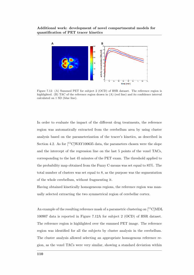
Additional work: development of novel compartmental models forquantification of PET tracer kinetics
Figure 7.12: (A) Summed PET for subject 2 (OCD) of HSR dataset. The reference region ishighlighted. (B) TAC of the reference region drawn in (A) (red line) and its confidence intervalcalculated on 1 SD (blue line).
In order to evaluate the impact of the different drug treatments, the reference
region was automatically extracted from the cerebellum area by using cluster
analysis based on the parameterization of the tracer’s kinetics, as described in
Section 4.2. As for [11C]WAY100635 data, the parameters chosen were the slope
and the intercept of the regression line on the last 5 points of the voxel TACs,
corresponding to the last 45 minutes of the PET exam. The threshold applied to
the probability map obtained from the Fuzzy C-means was set equal to 85%. The
total number of clusters was set equal to 8, as the purpose was the segmentation
of the whole cerebellum, without fragmenting it.
Having obtained kinetically homogeneous regions, the reference region was man-
ually selected extracting the two symmetrical region of cerebellar cortex.
An example of the resulting reference mask of a parametric clustering on [11C]MDL
100907 data is reported in Figure 7.12A for subject 2 (OCD) of HSR dataset.
The reference region is highlighted over the summed PET image. The reference
region was identified for all the subjects by cluster analysis in the cerebellum.
The cluster analysis allowed selecting an appropriate homogenous reference re-
gion, as the voxel TACs were very similar, showing a standard deviation within
110

7.2 Modeling [11C]MDL100907 dataset
Figure 7.13: Mean of the extracted reference region TACs (normalized to peak) of the twodatasets: (A) Imperial dataset, control subjects at baseline (red squares) and after administra-tion of mirtazapine (blue squares), (B) HSR dataset, control subjects at baseline (test and retest:black and green crosses) and OCD subjects at baseline (red circles) and after administration ofSSRI (violet circles).
the region lower than 5% (Figure 7.12B).
In Figure 7.13 the means of the extracted reference region TACs (normalized to
peak) of the two datasets are presented. Figure 7.13A reports the curves of the
control subjects at baseline (red squares) and after administration of mirtazapine
(blue squares) for the Imperial dataset, whereas in Figure 7.13B the curves of
the control subjects at baseline (test and retest: black and green crosses) and for
OCD subjects at baseline (red circles) and after administration of SSRI (violet
circles) for the HSR dataset are reported.
The reference region showed no changes in the kinetics for the baseline condition,
neither between patients and control subjects (HSR dataset, Figure 7.13B), nor
between the two datasets. From a comparison between Figure 7.13A and Figure
7.13B it can be seen that the kinetics are similar, even if there is a slight shift
between the two curves, and the mean ratio between the two reference TACs is
0.99 ± 0.11.
After administration of mirtazapine, there was a change in the kinetics of the
cortical regions, while this change did not occur in the reference region (Imperial
dataset, Figure 7.13A, as already found in [78] and [92]).
111
Additional work: development of novel compartmental models forquantification of PET tracer kinetics
Instead after administration of SSRI, there was an alteration in the reference
kinetic (Figure 7.13B), while the kinetic of the other regions remained unaltered.
To the best of the author’s knowledge, this is the first study which assessed the
validity of the cerebellum as reference region for [11C]MDL100907 after adminis-
tration of SSRI in humans.
On the basis of the results obtained, it was not possible to define clearly the causes
for this difference in the reference kinetics, but it is hypothesized that there could
be a metabolism and/or protein binding dependent effect that can be visible only
in the reference region using an high affinity tracer as [11C]MDL100907 because
of the small exchangeable compartment of the reference itself.
This finding strongly indicates that cerebellum cannot be used as true refer-
ence region in presence of pharmacological treatment that potentially modifies
metabolic enzymes like SSRI ([99], [100]).
112

Chapter 8
Overall discussion
8.1 Compartmental modeling at voxel level
Compartmental modeling represents the gold standard in PET quantification and
the methodologies developed aim to use compartmental modeling to quantify
PET images at voxel level. In both cases, a hierarchical approach was imple-
mented, using the information obtained at ROI level as a priori information for
the estimation process at voxel level.
In H-MAP the method uses a linear or linearized compartmental model, which
is then solved with a MAP estimator.
In H-BFM, the compartmental model is solved at voxel level in its non linear
version applying BFMs for PET quantification.
Both methodologies, as described in Chapter 2, can be applied to any PET re-
ceptor compartmental model.
H-MAP was applied to a linearized mono-compartmental model, whereas H-BFM
was applied to a 2 tissue compartmental model.
If the methods were to be applied to different models, no effect on the computa-
tional time is to be expected. In fact, in the case of H-MAP, the method can be
applied on any linear or linearized model, and the size of the state matrix would
have no impact on the time required for the estimate.
113

Overall discussion
H-BFM was already applied on one of the more complex model that is used in
receptor studies, and the eventual addition of a trapping component would not
represent a problem as it would just imply an addition of a linear component to
the estimation, without any effect on the grid definition and on the computation
cost.
On the contrary, the application of H-BFM to a simpler model (as for example
a 1T model, or the model presented in Section 7.1) would imply the definition
of only one grid, from the sampling of the Gaussian distribution obtained from
the ROI estimates, with the advantage of being able to sample on a denser grid,
with no impact on the computational cost.
8.2 Comparison of the novel methods with existing
methodologies
As it has been described in Chapter 1, there are other methodologies available
for quantification at the voxel level based on compartmental modeling.
The graphical methods (Patlak and Logan plot) allow fast estimation of the pa-
rameters of interest. For both methods, though, it is possible to estimate only a
macroparameter, with no information on the singular kinetic parameters, unless
a model structure is assumed. Moreover, estimates obtained using the Logan
approach are affected by bias, both at the ROI and voxel level ([30]).
Likelihood estimation in graphical analysis ([83]) and Empirical Bayesian esti-
mation in graphical analysis ([33]) are two alternative approaches developed to
eliminate the bias of the Logan plot results, but both of them still estimate only
one system parameter. Moreover, the model used is not linear and thus the meth-
ods are not appropriate for voxel-wise PET quantification.
In the linear and non linear ridge regression with spatial constraints ([23], [26])
114

8.2 Comparison of the novel methods with existing methodologies
the a priori information is provided for each voxel by the TACs of the voxels in
its neighborhood, using thus only a local prior. The method requires two itera-
tions of the regression analysis, making it appropriate only for linear models, as
the computational cost would be too high for clinical routine use in case of non
linear models.
BFMs and spectral analysis both require an a priori definition of a grid, which
is user-defined and fixed for all brain voxels. The choice of the grid can heavily
penalize the results and can lead to bias in the final estimates, which can also be
affected by the presence of noise in the data ([95]). Moreover spectral analysis
allow the estimation only of macro parameters, and the relation of these param-
eters to measures of the physiological process of interest is possible only with
knowledge of the biochemical properties of the tracer and with the definition of
the model structure.
All the methods described above present critical drawbacks which are instead
overcome with the novel approaches proposed in this work.
In fact the methods developed are user-independent and allow a fast, precise and
accurate estimation of the parameters of interest. Moreover, one of the main
advantage of compartmental modeling at voxel level compared to other method-
ologies is the possibility to obtain estimates for the microparameters, allowing a
much more detailed description of the receptor system and more insight in the
physiology.
One example is reported from the results presented in Section 6.2, i.e. H-BFM
applied to [11C]FLB457 and [11C]WAY100635 data.
In Figure 8.1 is presented the parametric maps for the parameter k3 and the Pear-
son’s correlation values between the average of the WNLLS and H-BFM estimates
are reported for each subject (H-BFM A and H-BFM C) for both [11C]FLB457
and [11C]WAY100635 datasets. It can be seen that the correlation values were
115
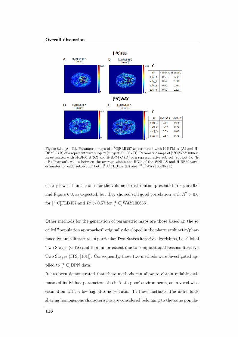
Overall discussion
Figure 8.1: (A - B). Parametric maps of [11C]FLB457 k3 estimated with H-BFM A (A) and H-BFM C (B) of a representative subject (subject 3). (C - D). Parametric maps of [11C]WAY100635k3 estimated with H-BFM A (C) and H-BFM C (D) of a representative subject (subject 4). (E- F) Pearson’s values between the average within the ROIs of the WNLLS and H-BFM voxelestimates for each subject for both [11C]FLB457 (E) and [11C]WAY100635 (F)
clearly lower than the ones for the volume of distribution presented in Figure 6.6
and Figure 6.8, as expected, but they showed still good correlation with R2 > 0.6
for [11C]FLB457 and R2 > 0.57 for [11C]WAY100635 .
Other methods for the generation of parametric maps are those based on the so
called ”population approaches” originally developed in the pharmacokinetic/phar-
macodynamic literature, in particular Two-Stages iterative algorithms, i.e. Global
Two Stages (GTS) and to a minor extent due to computational reasons Iterative
Two Stages (ITS, [101]). Consequently, these two methods were investigated ap-
plied to [11C]DPN data.
It has been demonstrated that these methods can allow to obtain reliable esti-
mates of individual parameters also in ’data poor’ environments, as in voxel-wise
estimation with a low signal-to-noise ratio. In these methods, the individuals
sharing homogenous characteristics are considered belonging to the same popula-
116

8.2 Comparison of the novel methods with existing methodologies
tion. These subjects are then studied together, thus allowing to obtain not only
the individual estimates but also a description of the population distribution.
Both can be applied to the voxel-wise quantification problem considering the vox-
els belonging to the same ROI as individuals of a population. The parameters
derived at ROI level were hypothesized representative of the expected model pa-
rameters values of the voxels composing the ROI itself and the standard deviation
of the parameters estimation error was assumed to represent the uncertainty of
the expected values.
8.2.1 Global Two Stage
This is an iterative method, in which the estimates for each voxel are iteratively
updated using both the population variability and the precision of the individual
estimates.
The initial estimates were obtained applying at voxel level 1T model linearized
(Eq. 2.20), which was solved with a linear least square estimator.
GTS was then applied in order to eliminate the bias introduced with the lin-
earization of the model.
There is no consensus on the criterion to use to stop iterations. Iterations were
stopped when the relative difference of each parameter between the current and
previous iteration was lower than 1% for at least 90% of the pixels included in
the considered population ([6]).
The same sensitiveness for the initial estimates already described in previous
works was found. As described in Section 4.1.1 [11C]DPN kinetics are nearly
irreversible and this represents a difficulty in the estimation of the parameters of
interest, in particular due to k2 which is estimated with a very low value and an
extremely narrow variability.
In fact the estimated variance of k2 is around 10-3 (min-1)2 while the population
117
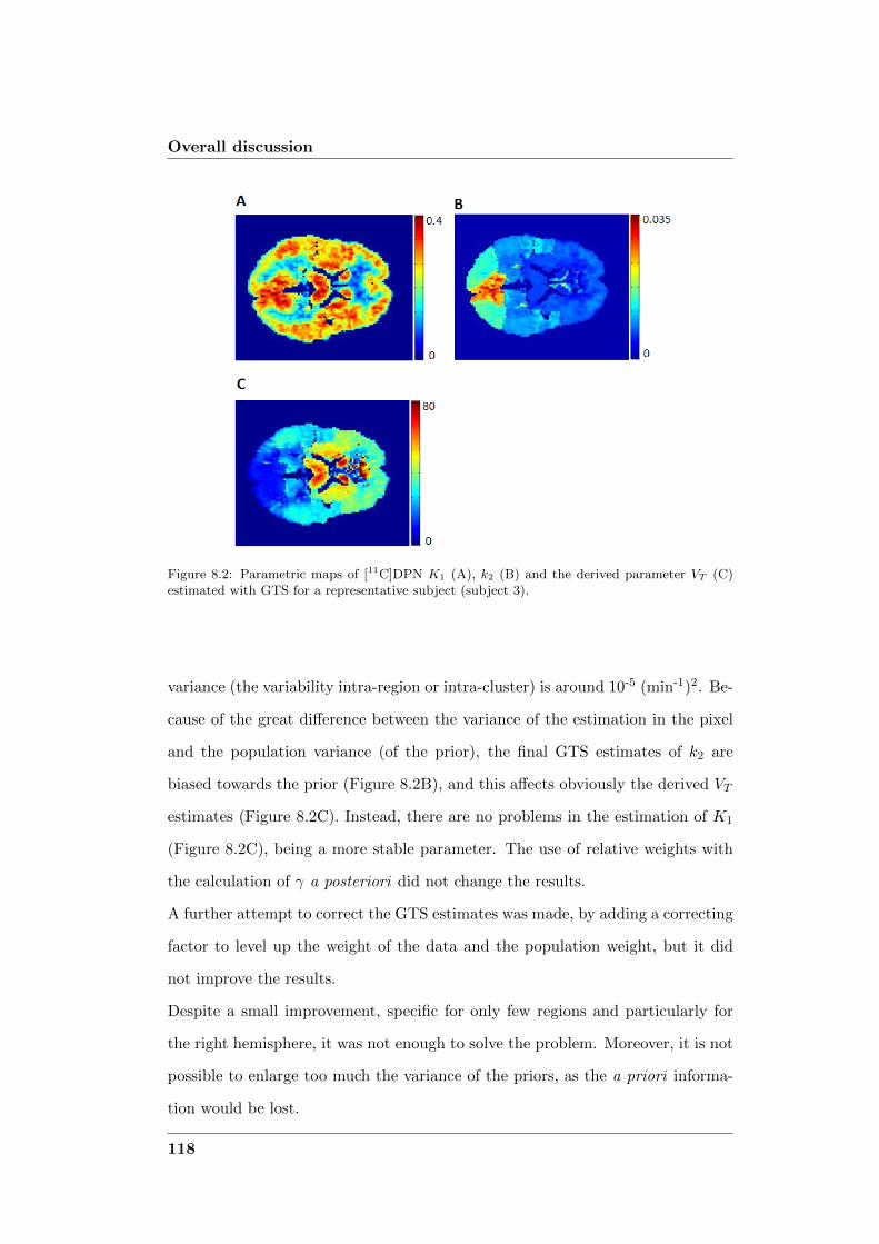
Overall discussion
Figure 8.2: Parametric maps of [11C]DPN K1 (A), k2 (B) and the derived parameter VT (C)estimated with GTS for a representative subject (subject 3).
variance (the variability intra-region or intra-cluster) is around 10-5 (min-1)2. Be-
cause of the great difference between the variance of the estimation in the pixel
and the population variance (of the prior), the final GTS estimates of k2 are
biased towards the prior (Figure 8.2B), and this affects obviously the derived VT
estimates (Figure 8.2C). Instead, there are no problems in the estimation of K1
(Figure 8.2C), being a more stable parameter. The use of relative weights with
the calculation of γ a posteriori did not change the results.
A further attempt to correct the GTS estimates was made, by adding a correcting
factor to level up the weight of the data and the population weight, but it did
not improve the results.
Despite a small improvement, specific for only few regions and particularly for
the right hemisphere, it was not enough to solve the problem. Moreover, it is not
possible to enlarge too much the variance of the priors, as the a priori informa-
tion would be lost.
118

8.2 Comparison of the novel methods with existing methodologies
Figure 8.3: Parametric map of [11C]DPN VT estimated with GTS for a representative subject(subject 3).
Using GTS, with the same settings as above, to estimate directly VT , i.e. defining
an unique prior based on the initial VT estimates, there was a slight improvement
(Figure 8.3). Nevertheless, the estimates were driven towards the priors, as the
variance of VT is calculated from the variance of k2, using the propagation the
rule.
Thus the same considerations already made in [6] and [32] apply also here: if
the initial estimates are robust, GTS allows for an improvement of the final es-
timates. But if the initial estimates are not adequate, GTS is unable to provide
good results.
8.2.2 Iterative Two Stage
ITS is an iterative method in which the individual estimates are updated using a
MAP estimator, using as empirical prior the mean and variance of the population
(i.e. the ROI which the voxel belongs to).
Applied by [101] to ROI curves it gave very promising results.
The initial estimates were obtained applying LEGA (Eq. 5.1) at voxel level,
solved with WNLLS, as it has been demonstrated that LEGA provides good re-
sults on ROI level, but it fails at pixel level ([83], [85]).
119
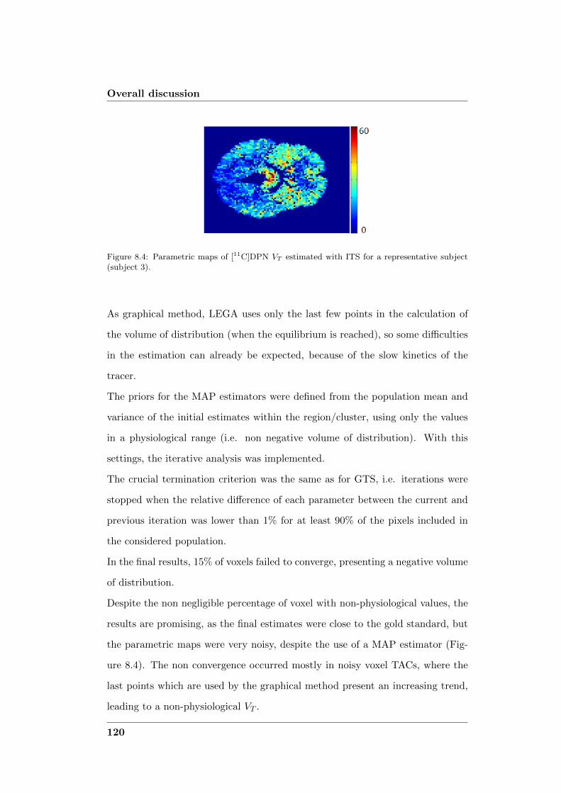
Overall discussion
Figure 8.4: Parametric maps of [11C]DPN VT estimated with ITS for a representative subject(subject 3).
As graphical method, LEGA uses only the last few points in the calculation of
the volume of distribution (when the equilibrium is reached), so some difficulties
in the estimation can already be expected, because of the slow kinetics of the
tracer.
The priors for the MAP estimators were defined from the population mean and
variance of the initial estimates within the region/cluster, using only the values
in a physiological range (i.e. non negative volume of distribution). With this
settings, the iterative analysis was implemented.
The crucial termination criterion was the same as for GTS, i.e. iterations were
stopped when the relative difference of each parameter between the current and
previous iteration was lower than 1% for at least 90% of the pixels included in
the considered population.
In the final results, 15% of voxels failed to converge, presenting a negative volume
of distribution.
Despite the non negligible percentage of voxel with non-physiological values, the
results are promising, as the final estimates were close to the gold standard, but
the parametric maps were very noisy, despite the use of a MAP estimator (Fig-
ure 8.4). The non convergence occurred mostly in noisy voxel TACs, where the
last points which are used by the graphical method present an increasing trend,
leading to a non-physiological VT .
120
8.3 Development of an alternative clustering algorithm
Attempts to ameliorate the final parametric maps did not succeed, as for example
applying GTS as smoothing filter, due to the big difference between the variance
of the data and the variance of the priors.
It is thus necessary to modify the method, but the problem it is not trivial. This
represents still an open issue and it will require an ad hoc solution.
8.3 Development of an alternative clustering algorithm
An additional but not less important result is the development of a new clustering
approach which allows the segmentation of the brain volume even for PET data
with high level of noise, without effect on the time required (the whole process
does not require more than 20 min, when the k-means applied to the whole voxel
TACs does not take less than 10 min).
This new approach was used for the ROI extraction for [11C]WAY100635 , [11C]SCH
442416 and [11C]MDL100907 data. Moreover, it was applied on [11C]MDL100907
data to select an appropriate homogenous reference region from the cerebellum.
In general, as described in Section 6.3, the way to derive the priors did not affect
the final results: the images did not differ qualitatively, and the average percent-
age difference of estimates was in general less than 3%, for all the datasets and
both H-MAP and H-BFM. For this reason, it can be inferred that priors defined
in such a way are appropriate and allow a robust estimation of the model param-
eters.
The number of ROIs and clusters (when segmenting using anatomical or func-
tional information respectively) had an effect on the quality of the final parametric
maps. The BrainAtlas was composed by more than 70 ROIs and resulted in re-
liable estimates.
121
Overall discussion
The use of a too rich or too poor atlas in terms of ROIs will imply less informa-
tive priors and consequently too noisy or too smoothed, respectively, parametric
maps.
In particular, the consequence in using an atlas with a relevant richer number of
ROIs will be a parametric map of the same quality of one obtained with conven-
tional least square estimators applied at voxel level. In general, from the results
obtained with an anatomical atlas with up to 83 regions, it would not be useful
an atlas very detailed, with a number of regions bigger than 100 (which would be
smaller and better defined), because the priors would be less informative resulting
in noisier estimates.
The same considerations hold when functional segmentation is used: if the num-
ber of clusters is set smaller than the optimal one, the priors will have bigger
SD and consequently there will be a smoothing on the estimates. If the number
of clusters is set bigger than the optimal one, the centroids of the clusters will
not be statistically different between each other and there will be repetition of
the kinetics. The optimal number of cluster (as defined in Section 6.3) was au-
tomatically selected as the greatest possible number which keeps the centroids
statistically different between each other. The statistical difference was tested
with the Wilcoxon’s test, as implemented in Matlab. In Figure 8.5 an example of
centroids obtained applying k-means to [11C]DPN data, setting K equal to the
optimal number of clusters (for this subject K = 7, Figure 8.5A) is presented.
In Figure 8.5B are presented also the centroids obtained clustering the cerebral
volume in 14 regions (overclustering). When the centroids of the clusters are not
statistically different between each other, there is repetition of the kinetics less
than a scale factor.
122

8.4 Conclusions
Figure 8.5: Example of centroids obtained with k-means applied on the whole voxel TACs of[11C]DPN (subject 3), subdivided in K = 7 clusters (optimal number, A) and K = 14 clusters(overclustering, B).
8.4 Conclusions
The main results of this work are the development of two methods for voxel-wise
quantification of PET data, H-MAP and H-BFM. The methods are fast and ro-
bust, and represent a good alternative for the generation of reliable parametric
maps. Applied to clinical data are expected to make it easier the detection also of
small/specific pathological areas. The first method led to a publication in Neu-
roimage ([12]), the second was presented during two international conferences
(BrainPET2011 and SNM2011) as oral contribute and a publication is ready to
be submitted.
The novel methods proposed have been already inserted in PIWAVE, a pre-
existing software for voxel-wise PET quantification originally developed by Im-
perial College of London.
Moreover, as collateral results, new compartmental models were developed for
[11C]SCH442416 and [11C]MDL100907 data and a new clustering approach which
allow segmenting the brain volume even for PET data with high level of noise was
implemented. This new method was also applied for the selection of the optimal
reference region for [11C]MDL100907 data.
123


Bibliography
[1] D. Feng, S. C. Huang, Z. Z. Wang, and D. Ho. An unbiased parametric imaging al-gorithm for nonuniformly sampled biomedical system parameter estimation. IEEETrans Med Imaging, 15:512–518, 1996.
[2] R. N. Gunn, A. A. Lammertsma, S. P. Hume, and V. J. Cunningham. Paramet-ric imaging of ligand-receptor binding in PET using a simplified reference regionmodel. Neuroimage, 6(4):279–87, 1997.
[3] Y. T. Hong and T. D. Fryer. Kinetic modelling using basis functions derived fromtwo-tissue compartmental models with a plasma input function: general principleand application to [18F]fluorodeoxyglucose positron emission tomography. Neu-roimage, 51:164–172, May 2010.
[4] Y. T. Hong, J. S. Beech, R. Smith, J. C. Baron, and T. D. Fryer. Paramet-ric mapping of [18F]fluoromisonidazole positron emission tomography using basisfunctions. J. Cereb. Blood Flow Metab., 31:648–657, Feb 2011.
[5] V. J. Cunningham and T. Jones. Spectral analysis of dynamic PET studies. JCereb Blood Flow Metab, 13(1):15–23, 1993.
[6] G. Tomasi, A. Bertoldo, and C. Cobelli. PET parametric imaging improved byglobal-two-stage method. Ann Biomed Eng, 37:419–427, Feb 2009.
[7] N. M. Alpert and F. Yuan. A general method of Bayesian estimation for parametricimaging of the brain. Neuroimage, 45:1183–1189, May 2009.
[8] A. Gjedde. Calculation of cerebral glucose phosphorylation from brain uptake ofglucose analogs in vivo: a re-examination. Brain Res., 257:237–274, Jun 1982.
[9] C. S. Patlak, R. G. Blasberg, and J. D. Fenstermacher. Graphical evaluation ofblood-to-brain transfer constants from multiple-time uptake data. J. Cereb. BloodFlow Metab., 3:1–7, Mar 1983.
[10] J. Logan, J. S. Fowler, N. D. Volkow, A. P. Wolf, S. L. Dewey, D. J. Schlyer, R. R.MacGregor, R. Hitzemann, B. Bendriem, and S. J. Gatley. Graphical analysis ofreversible radioligand binding from time-activity measurements applied to [N-11C-methyl]-(-)-cocaine PET studies in human subjects. J. Cereb. Blood Flow Metab.,10:740–747, Sep 1990.
[11] R.E. Carson, C. Cobelli, and L. Filkestein. The Mathematical Modeling of Metabolicand Endocrine Systems. Wiley, New York, 1993.
[12] G. Rizzo, F. E. Turkheimer, S. Keihaninejad, S. K. Bose, A. Hammers, andA. Bertoldo. Multi-Scale hierarchical generation of PET parametric maps: Ap-plication and testing on a [11C]DPN study. Neuroimage, 59:2485–2493, Feb 2012.
125

BIBLIOGRAPHY
[13] R. N. Gunn, S. R. Gunn, F. E. Turkheimer, J. A. Aston, and V. J. Cunningham.Positron emission tomography compartmental models: a basis pursuit strategy forkinetic modeling. J Cereb Blood Flow Metab, 22(12):1425–39, 2002.
[14] S. S. Kety. The theory and applications of the exchange of inert gas at the lungsand tissues. Pharmacol. Rev., 3:1–41, Mar 1951.
[15] L. Sokoloff, M. Reivich, C. Kennedy, M. H. Des Rosiers, C. S. Patlak, K. D.Pettigrew, O. Sakurada, and M. Shinohara. The [14C]deoxyglucose method for themeasurement of local cerebral glucose utilization: theory, procedure, and normalvalues in the conscious and anesthetized albino rat. J. Neurochem., 28:897–916,May 1977.
[16] M. A. Mintun, M. E. Raichle, M. R. Kilbourn, G. F. Wooten, and M. J. Welch. Aquantitative model for the in vivo assessment of drug binding sites with positronemission tomography. Ann. Neurol., 15:217–227, Mar 1984.
[17] G. Blomqvist, S. Pauli, L. Farde, L. Ericksson, A. Persson, and C. Halldin. PositronEmission Tomography in Clinical Research: Tracer Modelling and Radioreceptors(Developments in Nuclear Medicine). Springer, 1989.
[18] V. J. Cunningham, S. P. Hume, G. R. Price, R. G. Ahier, J. E. Cremer, and A. K.Jones. Compartmental analysis of diprenorphine binding to opiate receptors in therat in vivo and its comparison with equilibrium data in vitro. J. Cereb. Blood FlowMetab., 11:1–9, Jan 1991.
[19] S. P. Hume, R. Myers, P. M. Bloomfield, J. Opacka-Juffry, J. E. Cremer, R. G.Ahier, S. K. Luthra, D. J. Brooks, and A. A. Lammertsma. Quantitation of carbon-11-labeled raclopride in rat striatum using positron emission tomography. Synapse,12:47–54, Sep 1992.
[20] A. A. Lammertsma, C. J. Bench, S. P. Hume, S. Osman, K. Gunn, D. J.Brooks, and R. S. Frackowiak. Comparison of methods for analysis of clinical[11C]raclopride studies. J. Cereb. Blood Flow Metab., 16:42–52, Jan 1996.
[21] A. A. Lammertsma and S. P. Hume. Simplified reference tissue model for PETreceptor studies. Neuroimage, 4:153–158, Dec 1996.
[22] Claudio Cobelli and E.R. Carson. Introduction to modeling in physiology andmedicine. Academic Press series in biomedical engineering. Academic Press, SanDiego, 2008.
[23] Y. Zhou, S. C. Huang, and M. Bergsneider. Linear ridge regression with spatialconstraint for generation of parametric images in dynamic positron emission to-mography studies. IEEE Transactions on Nuclear Science, 48:125–130, Feb 2001.
[24] X. Dai, Z. Chen, and J. Tian. Performance evaluation of kinetic parameter esti-mation methods in dynamic FDG-PET studies. Nucl Med Commun, 32:4–16, Jan2011.
[25] F. E. Turkheimer, R. Hinz, R. N. Gunn, J. A. Aston, S. R. Gunn, and V. J.Cunningham. Rank-shaping regularization of exponential spectral analysis for ap-plication to functional parametric mapping. Phys Med Biol, 48(23):3819–41, 2003.
[26] Y. Zhou, S. C. Huang, M. Bergsneider, and D. F. Wong. Improved parametricimage generation using spatial-temporal analysis of dynamic PET studies. Neu-roimage, 15:697–707, Mar 2002.
126
BIBLIOGRAPHY
[27] A. Hammers, R. Allom, M. J. Koepp, S. L. Free, R. Myers, L. Lemieux, T. N.Mitchell, D. J. Brooks, and J. S. Duncan. Three-dimensional maximum probabilityatlas of the human brain, with particular reference to the temporal lobe. Hum BrainMapp, 19:224–247, Aug 2003.
[28] R. A. Koeppe, V. A. Holthoff, K. A. Frey, M. R. Kilbourn, and D. E. Kuhl.Compartmental analysis of [11C]flumazenil kinetics for the estimation of ligandtransport rate and receptor distribution using positron emission tomography. J.Cereb. Blood Flow Metab., 11:735–744, Sep 1991.
[29] G. Blomqvist. On the construction of functional maps in positron emission tomog-raphy. J. Cereb. Blood Flow Metab., 4:629–632, Dec 1984.
[30] M. Slifstein and M. Laruelle. Models and methods for derivation of in vivo neu-roreceptor parameters with PET and SPECT reversible radiotracers. Nucl. Med.Biol., 28:595–608, Jul 2001.
[31] R. B. Innis, V. J. Cunningham, J. Delforge, M. Fujita, A. Gjedde, R. N. Gunn,J. Holden, S. Houle, S. C. Huang, M. Ichise, H. Iida, H. Ito, Y. Kimura, R. A.Koeppe, G. M. Knudsen, J. Knuuti, A. A. Lammertsma, M. Laruelle, J. Logan,R. P. Maguire, M. A. Mintun, E. D. Morris, R. Parsey, J. C. Price, M. Slifstein,V. Sossi, T. Suhara, J. R. Votaw, D. F. Wong, and R. E. Carson. Consensusnomenclature for in vivo imaging of reversibly binding radioligands. J Cereb BloodFlow Metab, 27(9):1533–1539, 2007.
[32] G. Tomasi, A. Bertoldo, C. Cobelli, N. Pavese, Y. F. Tai, A. Hammers, and F. E.Turkheimer. Global-two-stage filtering of clinical PET parametric maps: applica-tion to [(11)C]-(R)-PK11195. Neuroimage, 55:942–953, Apr 2011.
[33] F. Zanderigo, R. T. Ogden, A. Bertoldo, C. Cobelli, J. J. Mann, and R. V. Parsey.Empirical Bayesian estimation in graphical analysis: a voxel-based approach forthe determination of the volume of distribution in PET studies. Nucl. Med. Biol.,37:443–451, May 2010.
[34] J. B. MacQueen. Some methods for classification and analysis of multivariateobservations. In L. M. Le Cam and J. Neyman, editors, Proc. of the fifth BerkeleySymposium on Mathematical Statistics and Probability, volume 1, pages 281–297.University of California Press, 1967.
[35] J.C. Dunn. A fuzzy relative of the isodata process and its use in detecting compactwell-separated clusters. Journal of Cybernetics, 3:32–57, 1973.
[36] J.C. Bezdek. Pattern Recognition with Fuzzy Objective Function Algorithms.Plenum, 1981.
[37] Thomas Kailath, Ali H. Sayed, and Babak Hassibi. Linear Estimation. PrenticeHall, 2000.
[38] H. Vincent Poor. An Introduction to Signal Detection and Estimation (SpringerTexts in Electrical Engineering). Springer, 1994.
[39] A. Bertoldo, P. Vicini, G. Sambuceti, A. A. Lammertsma, O. Parodi, and C. Co-belli. Evaluation of compartmental and spectral analysis models of [(18)F]FDG ki-netics for heart and brain studies with PET. IEEE Trans Biomed Eng, 45(12):1429–48, 1998.
[40] B. M. Bell, J. V. Burke, and Schumitzky A. A relative weighting method forestimating parameters and variances in multiple data sets. Comput Stat DataAnal, 22:2: 119–135, 1996.
127

BIBLIOGRAPHY
[41] A. Hammers and A. Lingford-Hughes. Opioid imaging. Neuroimaging Clin. N.Am., 16:529–552, Nov 2006.
[42] A. K. Jones, S. K. Luthra, B. Maziere, V. W. Pike, C. Loc’h, C. Crouzel, A. Syrota,and T. Jones. Regional cerebral opioid receptor studies with [11C]diprenorphinein normal volunteers. J. Neurosci. Methods, 23:121–129, Mar 1988.
[43] B. Sadzot, J. C. Price, H. S. Mayberg, K. H. Douglass, R. F. Dannals, J. R. Lever,H. T. Ravert, A. A. Wilson, H. N. Wagner, and M. A. Feldman. Quantificationof human opiate receptor concentration and affinity using high and low specificactivity [11C]diprenorphine and positron emission tomography. J. Cereb. BloodFlow Metab., 11:204–219, Mar 1991.
[44] J. W. Lewis and S. M. Husbands. The orvinols and related opioids–high affinityligands with diverse efficacy profiles. Curr. Pharm. Des., 10:717–732, 2004.
[45] A. Hammers, M. C. Asselin, F. E. Turkheimer, R. Hinz, S. Osman, G. Hotton, D. J.Brooks, J. S. Duncan, and M. J. Koepp. Balancing bias, reliability, noise propertiesand the need for parametric maps in quantitative ligand PET: [(11)C]diprenorphinetest-retest data. Neuroimage, 38:82–94, Oct 2007.
[46] P. E. Kinahn and J. G. Rogers. Analytic 3D image reconstruction using all detectedevents. IEEE Trans Nucl Sci, 36:964–968, Feb 1989.
[47] I. S. Gousias, D. Rueckert, R. A. Heckemann, L. E. Dyet, J. P. Boardman, A. D.Edwards, and A. Hammers. Automatic segmentation of brain MRIs of 2-year-oldsinto 83 regions of interest. Neuroimage, 40:672–684, Apr 2008.
[48] F. Maes, A. Collignon, D. Vandermeulen, G. Marchal, and P. Suetens. Multimodal-ity image registration by maximization of mutual information. IEEE Trans MedImaging, 16:187–198, Apr 1997.
[49] A. K. Jones, V. J. Cunningham, S. K. Ha-Kawa, T. Fujiwara, Q. Liyii, S. K. Luthra,J. Ashburner, S. Osman, and T. Jones. Quantitation of [11C]diprenorphine cerebralkinetics in man acquired by PET using presaturation, pulse-chase and tracer-onlyprotocols. J. Neurosci. Methods, 51:123–134, Mar 1994.
[50] N. E. Anden and G. Stock. Effect of clozapine on the turnover of dopamine in thecorpus striatum and in the limbic system. J. Pharm. Pharmacol., 25:346–348, Apr1973.
[51] M. S. Lidow, G. V. Williams, and P. S. Goldman-Rakic. The cerebral cortex: a casefor a common site of action of antipsychotics. Trends Pharmacol. Sci., 19:136–140,Apr 1998.
[52] H. Takahashi, M. Higuchi, and T. Suhara. The role of extrastriatal dopamine D2receptors in schizophrenia. Biol. Psychiatry, 59:919–928, May 2006.
[53] J. M. Stone, J. M. Davis, S. Leucht, and L. S. Pilowsky. Cortical dopamine D2/D3receptors are a common site of action for antipsychotic drugs–an original patientdata meta-analysis of the SPECT and PET in vivo receptor imaging literature.Schizophr Bull, 35:789–797, Jul 2009.
[54] H. Olsson, C. Halldin, C. G. Swahn, and L. Farde. Quantification of [11C]FLB 457binding to extrastriatal dopamine receptors in the human brain. J. Cereb. BloodFlow Metab., 19:1164–1173, Oct 1999.
[55] C. Halldin, L. Farde, T. Hogberg, N. Mohell, H. Hall, T. Suhara, P. Karlsson,Y. Nakashima, and C. G. Swahn. Carbon-11-FLB 457: a radioligand for extrastri-atal D2 dopamine receptors. J. Nucl. Med., 36:1275–1281, Jul 1995.
128
BIBLIOGRAPHY
[56] A. J. Montgomery, P. Stokes, Y. Kitamura, and P. M. Grasby. Extrastriatal D2and striatal D2 receptors in depressive illness: pilot PET studies using [11C]FLB457 and [11C]raclopride. J Affect Disord, 101:113–122, Aug 2007.
[57] H. Olsson and L. Farde. Potentials and pitfalls using high affinity radioligands inPET and SPET determinations on regional drug induced D2 receptor occupancy–asimulation study based on experimental data. Neuroimage, 14:936–945, Oct 2001.
[58] D. Baldwin and S. Rudge. The role of serotonin in depression and anxiety. IntClin Psychopharmacol, 9 Suppl 4:41–45, Jan 1995.
[59] J. N. Joyce, A. Shane, N. Lexow, A. Winokur, M. F. Casanova, and J. E. Kleinman.Serotonin uptake sites and serotonin receptors are altered in the limbic system ofschizophrenics. Neuropsychopharmacology, 8:315–336, Jun 1993.
[60] L. Farde, H. Ito, C. G. Swahn, V. W. Pike, and C. Halldin. Quantitative analysesof carbonyl-carbon-11-WAY-100635 binding to central 5-hydroxytryptamine-1Areceptors in man. J. Nucl. Med., 39:1965–1971, Nov 1998.
[61] V. W. Pike, J. A. McCarron, A. A. Lammertsma, S. Osman, S. P. Hume, P. A. Sar-gent, C. J. Bench, I. A. Cliffe, A. Fletcher, and P. M. Grasby. Exquisite delineationof 5-HT1A receptors in human brain with PET and [carbonyl-11 C]WAY-100635.Eur. J. Pharmacol., 301:5–7, Apr 1996.
[62] R. V. Parsey, M. Slifstein, D. R. Hwang, A. Abi-Dargham, N. Simpson,O. Mawlawi, N. N. Guo, R. Van Heertum, J. J. Mann, and M. Laruelle. Vali-dation and reproducibility of measurement of 5-HT1A receptor parameters with[carbonyl-11C]WAY-100635 in humans: comparison of arterial and reference tiss-sue input functions. J. Cereb. Blood Flow Metab., 20:1111–1133, Jul 2000.
[63] R. M. Moresco, S. Todde, S. Belloli, P. Simonelli, A. Panzacchi, M. Rigamonti,M. Galli-Kienle, and F. Fazio. In vivo imaging of adenosine A2A receptors inrat and primate brain using [11C]SCH442416. Eur J Nucl Med Mol Imaging,32(4):405–413, 2005.
[64] S. N. Schiffmann, G. Fisone, R. Moresco, R. A. Cunha, and S. Ferre. AdenosineA2A receptors and basal ganglia physiology. Prog. Neurobiol., 83:277–292, Dec2007.
[65] S. Todde, R. M. Moresco, P. Simonelli, P. G. Baraldi, B. Cacciari, G. Spalluto,K. Varani, A. Monopoli, M. Matarrese, A. Carpinelli, F. Magni, M. G. Kienle, andF. Fazio. Design, radiosynthesis, and biodistribution of a new potent and selectiveligand for in vivo imaging of the adenosine A(2A) receptor system using positronemission tomography. J. Med. Chem., 43:4359–4362, Nov 2000.
[66] D. J. Brooks, S. Papapetropoulos, F. Vandenhende, D. Tomic, P. He, A. Coppell,and G. O’Neill. An open-label, positron emission tomography study to assessadenosine A2A brain receptor occupancy of vipadenant (BIIB014) at steady-statelevels in healthy male volunteers. Clin Neuropharmacol, 33:55–60, 2010.
[67] I.D. Hinz, R. Grachev, D.L. Cutler, J. Hunter, S. Osman, M. Doder, D.J. Brooks,and V.J. Cunningham. In-vivo quantification of A2A receptors in human brainwith [11C]SCH442416 and positron emission tomography. Molecular Imaging andBiology, 5:1656, May-June 2003.
[68] A. F. Ramlackhansingh, S. K. Bose, I. Ahmed, F. E. Turkheimer, N. Pavese, andD. J. Brooks. Adenosine 2A receptor availability in dyskinetic and nondyskineticpatients with Parkinson disease. Neurology, 76:1811–1816, May 2011.
129

BIBLIOGRAPHY
[69] I. B. Galazzo, S. K. Bose, A. F. Ramlackhansingh, I. Ahmed, N. Pavese, G. Rizzo,D. J. Brooks, F. E. Turkheimer, and A. Bertoldo. Kinetic modeling of the adeno-sine A2A subtype receptor radioligand [11C]SCH442416 in humans. Neuroimage,52:S178, Aug 2010.
[70] A. Pazos, R. Cortes, and J. M. Palacios. Quantitative autoradiographic mapping ofserotonin receptors in the rat brain. II. Serotonin-2 receptors. Brain Res., 346:231–249, Nov 1985.
[71] C. Lundkvist, C. Halldin, N. Ginovart, S. Nyberg, C. G. Swahn, A. A. Carr,F. Brunner, and L. Farde. [11C]MDL 100907, a radioligland for selective imagingof 5-HT(2A) receptors with positron emission tomography. Life Sci., 58:187–192,1996.
[72] H. Watabe, M. A. Channing, M. G. Der, H. R. Adams, E. Jagoda, P. Herscov-itch, W. C. Eckelman, and R. E. Carson. Kinetic analysis of the 5-HT2A ligand[11C]MDL 100,907. J. Cereb. Blood Flow Metab., 20:899–909, Jun 2000.
[73] H. Ito, S. Nyberg, C. Halldin, C. Lundkvist, and L. Farde. PET imaging of central5-HT2A receptors with carbon-11-MDL 100,907. J. Nucl. Med., 39:208–214, Jan1998.
[74] B. J. Jones and T. P. Blackburn. The medical benefit of 5-HT research. Pharmacol.Biochem. Behav., 71:555–568, Apr 2002.
[75] D. Perani, V. Garibotto, A. Gorini, R. M. Moresco, M. Henin, A. Panzacchi,M. Matarrese, A. Carpinelli, L. Bellodi, and F. Fazio. In vivo PET studyof 5HT(2A) serotonin and D(2) dopamine dysfunction in drug-naive obsessive-compulsive disorder. Neuroimage, 42:306–314, Aug 2008.
[76] H. P. Landolt and R. Wehrle. Antagonism of serotonergic 5-HT2A/2C receptors:mutual improvement of sleep, cognition and mood? Eur. J. Neurosci., 29:1795–1809, May 2009.
[77] S. Kasper, J. Tauscher, M. Willeit, M. Stamenkovic, A. Neumeister, B. Kufferle,C. Barnas, J. Stastny, N. Praschak-Rieder, L. Pezawas, M. de Zwaan, S. Quiner,W. Pirker, S. Asenbaum, I. Podreka, and T. Brucke. Receptor and transporterimaging studies in schizophrenia, depression, bulimia and Tourette’s disorder–implications for psychopharmacology. World J. Biol. Psychiatry, 3:133–146, Jul2002.
[78] R. Hinz, Z. Bhagwagar, P. J. Cowen, V. J. Cunningham, and P. M. Grasby. Val-idation of a tracer kinetic model for the quantification of 5-HT(2A) receptors inhuman brain with [(11)C]MDL 100,907. J. Cereb. Blood Flow Metab., 27:161–172,Jan 2007.
[79] S. A. Anttila and E. V. Leinonen. A review of the pharmacological and clinicalprofile of mirtazapine. CNS Drug Rev, 7:249–264, 2001.
[80] T. S. Furey, N. Cristianini, N. Duffy, D. W. Bednarski, M. Schummer, and D. Haus-sler. Support vector machine classification and validation of cancer tissue samplesusing microarray expression data. Bioinformatics, 16:906–914, Oct 2000.
[81] R. Hinz and F.E. Turkheimer. Determination of tracer arrival delay with spectralanalysis. IEEE Trans Nucl Sci, 53(1):212–219, 2006.
[82] B. M. Mazoyer, R. H. Huesman, T. F. Budinger, and B. L. Knittel. Dynamic PETdata analysis. J Comput Assist Tomogr, 10:645–653, 1986.
130

BIBLIOGRAPHY
[83] R. T. Ogden. Estimation of kinetic parameters in graphical analysis of PET imagingdata. Stat Med, 22:3557–3568, Nov 2003.
[84] M. Laruelle. Modelling: when and why? Eur J Nucl Med, 26:571–572, Jun 1999.
[85] R. V. Parsey, R. T. Ogden, and J. J. Mann. Determination of volume of distributionusing likelihood estimation in graphical analysis: elimination of estimation bias. J.Cereb. Blood Flow Metab., 23:1471–1478, Dec 2003.
[86] J. Hirvonen, S. Aalto, V. Lumme, K. Nagren, J. Kajander, H. Vilkman, N. Hagel-berg, V. Oikonen, and J. Hietala. Measurement of striatal and thalamic dopamineD2 receptor binding with 11C-raclopride. Nucl Med Commun, 24:1207–1214, Dec2003.
[87] R. N. Gunn, P. A. Sargent, C. J. Bench, E. A. Rabiner, S. Osman, V. W. Pike,S. P. Hume, P. M. Grasby, and A. A. Lammertsma. Tracer kinetic modeling ofthe 5-HT1A receptor ligand [carbonyl-11C]WAY-100635 for PET. Neuroimage,8:426–440, Nov 1998.
[88] V. Oikonen, T. Allonen, K. Nagren, J. Kajander, and J. Hietala. Quantificationof [Carbonyl-(11)C]WAY-100635 binding: considerations on the cerebellum. Nucl.Med. Biol., 27:483–486, Jul 2000.
[89] R. V. Parsey, V. Arango, D. M. Olvet, M. A. Oquendo, R. L. Van Heertum, andJ. John Mann. Regional heterogeneity of 5-HT1A receptors in human cerebellumas assessed by positron emission tomography. J. Cereb. Blood Flow Metab., 25:785–793, Jul 2005.
[90] K. Varani, F. Portaluppi, S. Merighi, E. Ongini, L. Belardinelli, and P. A. Borea.Caffeine alters A2A adenosine receptors and their function in human platelets.Circulation, 99:2499–2502, May 1999.
[91] P. Svenningsson, C. Le Moine, G. Fisone, and B. B. Fredholm. Distribution,biochemistry and function of striatal adenosine A2A receptors. Prog. Neurobiol.,59:355–396, Nov 1999.
[92] P. S. Talbot, M. Slifstein, D. R. Hwang, Y. Huang, E. Scher, A. Abi-Dargham, andM. Laruelle. Extended characterisation of the serotonin 2A (5-HT2A) receptor-selective PET radiotracer 11C-MDL100907 in humans: quantitative analysis, test-retest reproducibility, and vulnerability to endogenous 5-HT tone. Neuroimage,59:271–285, Jan 2012.
[93] P. T. Meyer, Z. Bhagwagar, P. J. Cowen, V. J. Cunningham, P. M. Grasby, andR. Hinz. Simplified quantification of 5-HT2A receptors in the human brain with[11C]MDL 100,907 PET and non-invasive kinetic analyses. Neuroimage, 50:984–993, Apr 2010.
[94] M. E. Phelps, S. C. Huang, E. J. Hoffman, C. Selin, L. Sokoloff, and D. E. Kuhl.Tomographic measurement of local cerebral glucose metabolic rate in humans with(F-18)2-fluoro-2-deoxy-D-glucose: validation of method. Ann. Neurol., 6:371–388,Nov 1979.
[95] F. Turkheimer, R. M. Moresco, G. Lucignani, L. Sokoloff, F. Fazio, and K. Schmidt.The use of spectral analysis to determine regional cerebral glucose utilization withpositron emission tomography and [18F]fluorodeoxyglucose: theory, implementa-tion, and optimization procedures. J Cereb Blood Flow Metab, 14(3):406–22, 1994.
[96] W. H. Press, B. P. Flannery, S. A. Teukolsky, and W. T. Vetterling. NumericalRecipes: The Art of Scientific Computing. Cambridge University Press, 1986.
131
BIBLIOGRAPHY
[97] E. M. DiStefano, Landaw. Multiexponential, multicompartmental, and noncom-partmental modeling. I. methodological limitations and physiological interpreta-tions. Am J Physiol, 246(5 Pt 2):R651–64, 1984.
[98] M. Veronese, A. Bertoldo, S. Bishu, A. Unterman, G. Tomasi, C. B. Smith, andK. C. Schmidt. A spectral analysis approach for determination of regional ratesof cerebral protein synthesis with the L-[1-(11)C]leucine PET method. J. Cereb.Blood Flow Metab., 30:1460–1476, Aug 2010.
[99] K. Brøsen, E. Skjelbo, B. B. Rasmussen, H. E. Poulsen, and S. Loft. Fluvoxamineis a potent inhibitor of cytochrome P4501A2. Biochem. Pharmacol., 45:1211–1214,Mar 1993.
[100] K. Brøsen. The pharmacogenetics of the selective serotonin reuptake inhibitors.Clin Investig, 71:1002–1009, Dec 1993.
[101] A. Bertoldo, G. Sparacino, and C. Cobelli. ”Population” approach improves pa-rameter estimation of kinetic models from dynamic PET data. IEEE Trans MedImaging, 23:297–306, Mar 2004.
132