3D Scene Understanding by Voxel-CRF

Byung-soo KimUniversity of Michiganbsookim@umich.edu

Pushmeet KohliMicrosoft Research Cambridge

pkohli@microsoft.com

Silvio SavareseStanford University

ssilvio@stanford.edu

AbstractScene understanding is an important yet very challeng-

ing problem in computer vision. In the past few years, re-searchers have taken advantage of the recent diffusion ofdepth-RGB (RGB-D) cameras to help simplify the problemof inferring scene semantics. However, while the added 3Dgeometry is certainly useful to segment out objects with dif-ferent depth values, it also adds complications in that the3D geometry is often incorrect because of noisy depth mea-surements and the actual 3D extent of the objects is usuallyunknown because of occlusions. In this paper we proposea new method that allows us to jointly refine the 3D recon-struction of the scene (raw depth values) while accuratelysegmenting out the objects or scene elements from the 3Dreconstruction. This is achieved by introducing a new modelwhich we called Voxel-CRF. The Voxel-CRF model is basedon the idea of constructing a conditional random field overa 3D volume of interest which captures the semantic and3D geometric relationships among different elements (vox-els) of the scene. Such model allows to jointly estimate (1) adense voxel-based 3D reconstruction and (2) the semanticlabels associated with each voxel even in presence of par-tial occlusions using an approximate yet efficient inferencestrategy. We evaluated our method on the challenging NYUDepth dataset (Version 1 and 2). Experimental results showthat our method achieves competitive accuracy in inferringscene semantics and visually appealing results in improvingthe quality of the 3D reconstruction. We also demonstratean interesting application of object removal and scene com-pletion from RGB-D images.

1. IntroductionUnderstanding the geometric and semantic structure of

a scene (scene understanding) is a critical problem in vari-ous research fields including computer vision, robotics, andaugmented reality. For instance, consider a robot in the in-door scene shown in the Fig. 1. In order to safely navigatethrough the environment, the robot must perceive the freespace of the scene accurately (geometric structure). More-over, in order for the robot to effectively interact with theenvironment (e.g., to place a bottle on a table), it must rec-ognize the objects in the scene (semantic structure).

Several methods have been proposed to solve the prob-lem of scene understanding using a single RGB (2D) im-

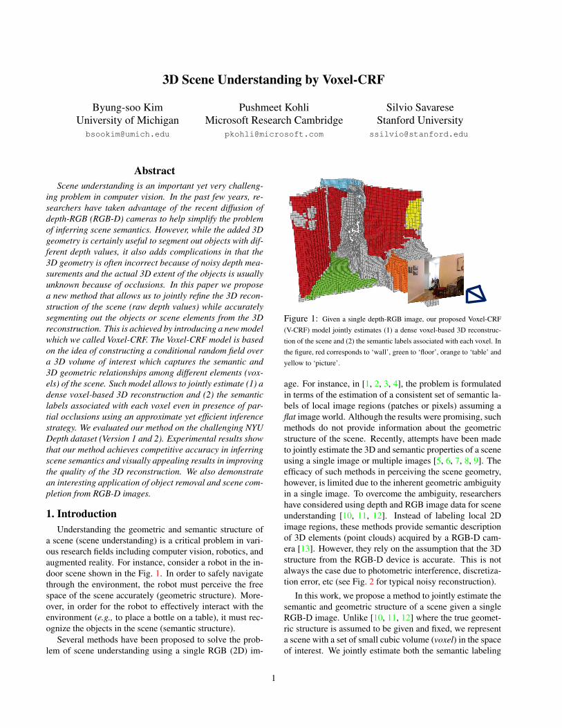
Figure 1: Given a single depth-RGB image, our proposed Voxel-CRF(V-CRF) model jointly estimates (1) a dense voxel-based 3D reconstruc-tion of the scene and (2) the semantic labels associated with each voxel. Inthe figure, red corresponds to ‘wall’, green to ‘floor’, orange to ‘table’ andyellow to ‘picture’.

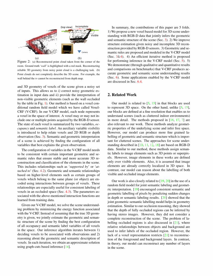
age. For instance, in [1, 2, 3, 4], the problem is formulatedin terms of the estimation of a consistent set of semantic la-bels of local image regions (patches or pixels) assuming aflat image world. Although the results were promising, suchmethods do not provide information about the geometricstructure of the scene. Recently, attempts have been madeto jointly estimate the 3D and semantic properties of a sceneusing a single image or multiple images [5, 6, 7, 8, 9]. Theefficacy of such methods in perceiving the scene geometry,however, is limited due to the inherent geometric ambiguityin a single image. To overcome the ambiguity, researchershave considered using depth and RGB image data for sceneunderstanding [10, 11, 12]. Instead of labeling local 2Dimage regions, these methods provide semantic descriptionof 3D elements (point clouds) acquired by a RGB-D cam-era [13]. However, they rely on the assumption that the 3Dstructure from the RGB-D device is accurate. This is notalways the case due to photometric interference, discretiza-tion error, etc (see Fig. 2 for typical noisy reconstruction).

In this work, we propose a method to jointly estimate thesemantic and geometric structure of a scene given a singleRGB-D image. Unlike [10, 11, 12] where the true geomet-ric structure is assumed to be given and fixed, we representa scene with a set of small cubic volume (voxel) in the spaceof interest. We jointly estimate both the semantic labeling

1

(a)

Camera

Visible

Incomplete (top view)

(b)Figure 2: (a) Reconstructed point cloud taken from the corner of theroom. Ground truth ‘wall’ is highlighted with a red mask. Reconstructingreliable 3D geometry from noisy point cloud is a challenging task. (b)Point clouds do not completely describe the 3D scene. For example, thewall behind the tv cannot be reconstructed from depth map.

and 3D geometry of voxels of the scene given a noisy setof inputs. This allows us to i) correct noisy geometric es-timation in input data and ii) provide the interpretation ofnon-visible geometric elements (such as the wall occludedby the table in Fig. 1). Our method is based on a voxel con-ditional random field model which we have called Voxel-CRF (V-CRF). In our V-CRF model, each node representsa voxel in the space of interest. A voxel may or may not in-clude one or multiple points acquired by the RGB-D sensor.The state of each voxel is summarized by two variables, oc-cupancy and semantic label. An auxiliary variable visibilityis introduced to help relate voxels and 2D RGB or depthobservation (Sec. 3). Semantic and geometric interpretationof a scene is achieved by finding the configuration of allvariables that best explains the given observation.

The configuration of variables in the V-CRF model needsto be consistent with certain important geometric and se-mantic rules that ensure stable and more accurate 3D re-construction and classification of the elements in the scene.This includes relationships such as ‘supported by’ or ‘at-tached to’ (Sec. 4.2). Geometric and semantic relationshipsbased on higher-level elements such as certain groups ofvoxels which belong to the same plane (or object) are en-coded using interactions between groups of voxels. Theserelationships are especially useful for consistent labeling ofvoxels in an occluded space (Sec. 4.3). The parameters as-sociated with the above-mentioned interaction functions arelearned from training data.

Given our V-CRF model, we solve the scene understand-ing problem by minimizing the energy function associatedwith the V-CRF. Instead of assuming that the true 3D geom-etry is given, we jointly estimate the geometric and seman-tic structure of the scene by finding the best configurationof all occupancy and semantic label variables of all voxelsin the space. Our inference algorithm iterates between 1)deciding voxels to be associated with observations and 2)reasoning about the geometric and semantic description ofvoxels. In each iteration, we obtain an approximate solutionusing graph-cuts based inference [14].

In summary, the contributions of this paper are 5 folds.1) We propose a new voxel based model for 3D scene under-standing with RGB-D data that jointly infers the geometricand semantic structure of the scene (Sec. 3). 2) We improvestructure estimation given noisy and incomplete 3D recon-struction provided by RGB-D sensors. 3) Geometric and se-mantic rules are proposed and modeled in the V-CRF model(Sec. 3&4). 4) An efficient iterative method is proposedfor performing inference in the V-CRF model (Sec. 5). 5)We demonstrate (through qualitative and quantitative resultsand comparisons on benchmarks) that V-CRF produces ac-curate geometric and semantic scene understanding results(Sec. 6). Some applications enabled by the V-CRF modelare discussed in Sec. 6.4.

2. Related Work

Our model is related to [5, 15] in that blocks are usedto represent 3D space. On the other hand, unlike [5, 15],our blocks are defined at a fine resolution that enables us tounderstand scenes (such as cluttered indoor environments)in more detail. The methods proposed in [16, 17, 7] arealso relevant to our work. These methods analyze geomet-ric properties of the underlying scene and infer free space.However, our model can produce more fine grained la-belling of geometric and semantic structure which is impor-tant for cluttered scenes. The approaches for scene under-standing described in [10, 11, 12, 18] are based on RGB-Ddata. Similar to our method, these methods assign seman-tic labels to image elements such as 3D points or superpix-els. However, image elements in these works are definedonly over visible elements. Also, it is assumed that imageelements are already correctly localized in 3D space. Incontrast, our model can reason about the labelling of bothvisible and occluded image elements.

Our work is also closely related to [19, 20] in the use of arandom field model for joint semantic labeling and geomet-ric interpretation. [19] encouraged consistent semantic andgeometric labelling of pixels by penalizing sudden changesin depth or semantic labeling results. [20] showed that thejoint geometric-semantic labelling model helps in geometryestimation. Similar to our occlusion reasoning, they showedthat the depth of fully occluded regions can be inferred byhaving stereo images. However, they did not consider acomplete reconstruction of the scene. The problem of la-belling occluded regions is also discussed in [21], whererelative relationships between objects and background areused to infer labels of the occluded region. However, thelack of a voxel representation restricts [21] to reconstruc-tion of the foreground and background layers. In contrast,in theory, our model can reconstruct any number of layersin the scene.

Camera Image

(a) (b)

Figure 3: Ambiguity of assigning image observations to the voxels in aview ray. Five voxels with green outline are the ground truth voxels in acorrect place. (a) For the successful cases, the voxel can be reconstructedfrom a depth data. (b) Unfortunately, due to noisy depth data, incorrectvoxels are reconstructed in many cases.

3. Voxel-CRFWe now describe the Voxel-CRF (V-CRF) model. We

represent the semantic and geometric structure of the scenewith a 3D lattice where each cell of the lattice is a voxel. V-CRF is defined over a graph G = (V, E , C), where V are ver-tices representing voxels, edges E connect horizontally orvertically adjacent pairs of vertices, cliques C are groups ofvoxels which are related, e.g., voxels on the same 3D plane,or voxels that are believed to belong to an object (throughan object detection bounding box). The state of each voxelis described with a structured label `i = (oi, si) and the vis-ibility vi. The first variable oi represents voxel occupancy;i.e., it indicates whether voxel i is empty (oi = 0) or occu-pied (oi = 1). The second variable si indicates the index ofsemantic class the voxel belong to; i.e., si ∈ {1, · · · , |S|}if the voxel is occupied (oi = 1), or si = ø if oi = 0, where|S| is the number of semantic classes (e.g., table, wall, ...).Estimation of the structured label L = {`i} over the V-CRFmodel produces a geometric and semantic interpretation ofthe scene.

The variable vi encodes the visibility of a voxel i wherevi = 1 and vi = 0 indicate whether the voxel is visibleor non-visible, respectively. Any given ray from the cam-era touches a single visible (occupied) voxel. Due to thehigh amount of noise in the RGB-D sensor, it is difficult tounambiguously assign 2D observations (image appearanceand texture) to voxels in 3D space (see Fig. 3 for an illus-tration). The visibility variables vi allow us to reason aboutthis ambiguity. Provided that we know which single voxelis visible on the viewing-ray, we can assign the 2D imageobservation to the corresponding voxel. Since visibility is afunction of occupancy, and vice versa, we infer the optimalconfiguration of the two in an iterative procedure.

V-CRF can be considered as a generalization of ex-isting CRF-based models for scene understanding in 3D[10, 11, 12], where {oi} and {vi} are assumed to be given,and semantic labels {si} are inferred only for visible andoccupied scene elements. In contrast, V-CRF model is moreflexible by having oi and vi as random variables, and thisenables richer scene interpretation by i) estimating occludedregions, e.g., (oi, si)=(occupied,table), vi= occluded, and ii)correcting noisy depth data.

4. Energy FunctionGiven a graph G, we aim to find V ∗ = {v∗i } and L∗ =

{`∗i } that minimize the energy function E(V,L,O), whereO = {C, I,D}, C is the known camera parameters, I is theobservation from a RGB image, and D is the observationfrom a depth map. The energy function can be written asa sum of potential functions defined over individual, pairs,and group of voxels as: E(V,L,O) =∑i

φu(vi, `i, O) +∑i,j

φp(vi, `i, vj , `j , O) +∑c

φc(Vc, Lc, O)

(1)where i and j are indices of voxels and c is the index ofhigher-order cliques in a graph. The first term models theobservation cost for individual voxels, while the secondand third terms model semantic and geometric consistencyamong pairs and groups of voxels, respectively.4.1. Observation for Individual Voxels

The term φu represents the cost of the assignment (vi, `i)for a voxel i. We model the term for two different cases,when voxel i is occupied (oi = 1) and when it is empty(oi = 0).

φu(vi, `i, O) =

{k1 if oi = 1, si 6= ø

k2 if oi = 0, si = ø(2)

where k1 and k2 are defined as k1 =:

wu1 vi logP (si|O)−wu2 log fs(di−dmr(i))−wu3 log|Pi||Pmaxi | (3)

and k2 = −wu4 log(1− fs(di − dmr(i)))− wu5 log(1− |Pi||Pmaxi | ).

(4)When the voxel i is occupied (oi = 1), it is composed

of three terms. The first term incorporates the observationsP (si|O) from an image if it is visible (vi = 1), to estimatea structured label of the voxel. The second term modelsthe uncertainty in the depth value from the RGBD imagethrough a normal distribution fs ∼ N (0, σ2). Larger thedisparity between depth according to the data map valuedmr (i), which is value associated with a ray r(i) for a voxeli, and the voxel i’s depth di, more likely it is to be labeled asan empty state. The third term models the occupancy basedon density of 3D points in a voxel i. Note that there can bemore than one image pixel corresponding to a voxel. Wemeasure the ratio |Pi|/|Pmax

i |, which is the ratio betweenthe number of detected points in 3D cubical volume associ-ated with a voxel i over the maximum number of 3D pointsin a voxel i, i.e., the number of rays penetrating through avoxel i. If there is an object at voxel i, and the surface isperpendicular to the camera ray, the number of points is thelargest. If this ratio is small (i.e. few points), the energyfunction encourages oi = 0.

In the case the voxel i is empty (oi = 0), the energymodels the sensitivity of the sensor (first term) and the den-

sity of point clouds (second term). Different terms are bal-anced with weights wu

{·}, which are learned from the train-ing dataset as discussed in Sec. 5.4.2. Relating Pairs of Voxels

The pairwise energy terms penalize labellings of pairs ofvoxels that are geometrically or semantically inconsistent.Two different types of neighborhoods are considered to de-fine pairwise relationships between voxels: i) adjacent vox-els in 3D lattice structure, and ii) adjacent voxels in its 2Dprojection. The pairwise costs depend on visibility, spatialrelationship, and appearance similarity of a pair of voxels.Appearance similarity between a pair of voxels (e.g., color)is represented by cij which is a discretized color differencebetween voxels i and j, similar to [22]. If voxel j is emptyor occluded, we use ci, i.e. in this case the cost is the func-tion of the color of the visible voxel i. The pairwise cost onthe labelling of voxels also depends on their visibility andis defined as:φp(vi = 1, `i, vj = 1, `j) = wpw1 (sij , cij)T [`i 6= `j ] (5)

φp(vi = 0, `i, vj = 1, `j) = wpw2 (sij , cj)T [`i 6= `j ] (6)

φp(vi = 1, `i, vj = 0, `j) = wpw3 (sij , ci)T [`i 6= `j ] (7)

φp(vi = 0, `i, vj = 0, `j) = wpw4 , (8)

where T [·] is the indicator function, sij is a spatial relation-ship between voxels i and j. i and j are chosen differentlyfor 2D and 3D cases as discussed below. These functionspenalize if `i and `j are inconsistent. The exact penalty forinconsistent assignments depends on the relative spatial lo-cation sij and colors cij of the voxel pairs. wpw

{·}(sij , cij)are weights that are learned from the training data.

Adjacent pairs in 3D. For all adjacent pairs of vox-els, we specify their spatial relationship sij , where sij ∈{vertical, horizontal}. The color difference between iand j is also used to modulate the cost wpw

{·}(·), where wecluster color difference between two voxels as in [22], cij isthe index of a closest cluster.

Adjacent pairs in 2D. On top of adjacent voxels in 3D,the adjacency between a pair of voxels in the projected 2Dimages is formulated as pairwise costs. For example, occlu-sion boundaries are useful cues to distinguish voxels thatbelong to different objects; if two voxels are across a de-tected occlusion boundary (when projected in the view ofthe camera), they are likely to have different semantic la-bels. On the other hand, if two voxels across the boundaryare still close in 3D, they are likely to have a same semanticlabel. The relationship of voxels are automatically indexedas follows. First, we extract pairs of 2D pixels from 2DRGB images which are on the opposite side of the occlu-sion boundaries. The pair of 2D pixels are then projectedinto 3D voxels. From the training data, we collect the rel-ative surface feature between voxels i and j1 and clusterthem to represent different types of corners, depending on

1The surface feature for adjacent regions i and j is composed of surfacenorm, color, and height.

(a) (b) (c)Figure 4: (Best visible in a high resolution) (a) A detected plane using[23] is highlighted with the blue mask. Its convex hull is drawn with theyellow polygon and it includes both visible and occluded region of a planarsurface. (b) A group of voxels associated with the detected planar surface(top) and a group of voxels associated with the convex hull (bottom). Thevoxels in the convex hull not only enforce consistency for visible voxels,but also for occluded voxels. (c) V-CRF result: our model not only allowsthe labeling of visible voxels for TV (top), but also the labeling of theoccluded region corresponding to the ‘wall’. For visibility, we removedthe voxels corresponding to the TV. (bottom).

their geometric properties in 3D. Finally, the spatial indexsij indicates a cluster ID. We learn different weights for dif-ferent cluster automatically from the training data.

4.3. Relating Groups of VoxelsWe now introduce higher-order potentials that encode

the relationship among more than two voxels. The poten-tials enforce semantic and geometric consistency amongvoxels in a clique c ∈ VC of voxels that can be quite farfrom each other. The relationships for a group of voxels canbe represented using the Robust Pott’s model [1]. Differenttypes of 3D priors can be used, e.g., surface detection, ob-ject detection, or room layout estimation; however, in thiswork, we consider two types of voxel groups VC , 1) 3D sur-faces that are detected using a Hough voting based method[23] and 2) categorical object detections [24] as follows2.

3D Surfaces. The first type is the group of voxels thatbelong to a 3D surface (wall, tables etc). From the depthdata and its projected point clouds, we can identify 3D sur-faces [23] and these are useful to understand images for tworeasons. First, a surface is likely to belong to an object ora facet of the indoor room layout, and there is consistencyamong labels of voxels for a detected plane. Second, thepart of the plane occluded by other objects can be inferredby extending the plane to include the convex hull3 of the de-tected surface (See Fig. 4). According to the law of closureof Gestalt theory, both visible and invisible regions insidethis convex hull are likely to belong to the same object.

Object Detections. Object detection methods provide acue to define groups of voxels (bounding box) that take thesame label, as used for 2D scene understanding in [25, 4],where we grouped a set of visible voxels which fall inside

2Room layout estimation is not used due to heavy clutter in the evalu-ated dataset.

33D plane with smallest perimeter containing all the points associatedwith a detected surface.

in the object bounding box. We use off-the-shelf detectors,e.g., proposed in [24], to find 2D object bounding boxes andthen find the corresponding voxels in 3D to form a clique.

4.4. Relating Voxels in a Camera RayV-CRF model enforces that there is only one visible

voxel for each ray from a camera. This is enforced by thefollowing energy term.

φc(Vcr , Lcr , O) =

{0 if

∑i∈c vi = 1

∞ otherwise(9)

where cr is indices of voxels in a single ray.

5. Inference and LearningIn this section, we discuss our inference and learning

procedures. We propose an inference method where struc-tured labels {`i} and visibility labels {vi} are iteratively up-dated (Sec. 5.1). The parameters of the model are learnedusing Structural SVM framework [26] (Sec. 5.2).

5.1. InferenceWe find the most probable labelling ofL and V under the

model by minimizing the energy function Eq. 1. Efficiencyof the inference step is a key requirement for us as V-CRFis defined over a voxel space which can be much larger thanthe number of pixels in the image. We propose an efficientgraph-cut based approximate iterative inference procedurethat is described below.

In the tth iteration, we estimate the value of the visibil-ity variables Vt from Lt−1 by finding out the first occupiedvoxel in each ray from a camera. Given Vt, we solve the en-ergy minimization problem argminLE(Vt, L,O) instead ofEq. 1, and update Lt. This procedure is illustrated in Alg. 1.Note that, by fixing Vt, the energy (Eq. 1) becomes indepen-dent of V and can be minimized using graph-cut [1, 14].

1 Initialize Vt, t = 0.;2 Build a V-CRF with unary, pairwise and higher-order

potential terms, by fixing Vt.;3 (Scene understanding) SolveLt+1 = argminLE(Vt, L,O) with the graph-cutmethod;

4 (Updating visibility) From Lt+1, update Vt+1;5 Go back to Step. 2.;

Algorithm 1: Iterative inference process for L and V .

5.2. LearningThe energy function introduced in Sec. 4 is the sum

of unary, pairwise, and higher-order potentials. Since theweights W = (wu

{·}, wpw{·}, w

g{·}) are linear in the energy

function, we formulate the training problem as a structuralSVM problem [26].

Specifically, given N RGB-D images (In, Dn)n∈1∼Nand their corresponding ground truth labels Ln, we solvethe following optimization problem:

minW,ξ≥0

WTW + C∑n

ξn(L) (10)

s.t. ξn(L) = maxL(∆(L;Ln) + E(Ln|W )− E(L|W ))

where C controls the relative weights of the sum of the vio-lated terms {ξn(L)} with respect to the regularization term.∆(L;Ln) is the loss function for the visible voxels accord-ing to its structured label that guarantees larger loss whenL is more different from Ln. Note that the loss functioncan be decomposed into a sum of local losses on individualvoxels, and the violated terms can be efficiently inferred bythe graph-cut method. Similar to [4], stochastic subgradientdecent method is be used to solve Eq. 10.

6. ExperimentsWe evaluate our framework on two datasets [28, 12].

6.1. Implementation DetailsAppearance Term. For the appearance term P (si|O)

for visible voxels in Sec. 4.1, we incorporate responses of[2] and [27], which are state-of-the-art methods using 2Dand 3D features, respectively.

3D Surface Detection. We find groups of voxels com-posing 3D surfaces using off-the-shelf plane detector [23],which detects a number of planes from point clouds byhough voting in a parameterized space. Different types ofparameterized space can be used; in this work, we usedRandomzied Hough Voting. Please see [23] for details.

Object Detection. We use pre-trained DPM detector[24] Release 4 [29] to provide detections for higher-ordercliques. Among various semantic classes, we used reliabledetection results from sofa, chair, and tv/monitors.

Voxel Initialization. To build V-CRF model, the 3Dspace of interest is divided with voxels having size of(4cm)3 for testing. For training, voxels are divided into(8cm)3 for efficiency. Since the difference in resolution issmall we could use the relationships learned from the train-ing set on the test set with reasonable results. Initializationis performed by assigning appearance likelihood for eachpoint in a cloud to a voxel. Note that more than one pointfrom a cloud can be associated with a single voxel; for sim-plicity, we used averaged appearance likelihood responsesfrom multiple points for Eq. 2.

6.2. NYU DEPTH Ver. 1We first evaluate our framework on the NYU Depth

dataset Ver. 1 (NYUD-V1) [28], where pixelwise annota-tions are available for 13 classes. The dataset contains 2347images from 64 different indoor environments. We used thesame 10 random splits of training and testing set used in

(a) RGB image (b) Depth map (c) Point cloud (d) Ground Truth (e) [27] (f) V-CRF

Figure 5: Four typical examples show that the 3D geometry of the scene is successfully estimated by solving V-CRF model. Given (a) a RGB imageand (b) a depth map, (c) reconstructed 3D geometry (top view) suffers from noise and may not produce realistic scene understanding results. (d) Annotatedtop-view structured labels (occupied or not, semantic labels). (e) Results from other methods, e.g., [27]. (f) V-CRF achieves labeling and reconstructionresults that are closer to the ground truth than [27]. For instance, the empty space (hall) in the first image is successfully constructed with V-CRF, whereas[27] fails. Even with the error due to reflection of the mirror on the third example, V-CRF is capable of reconstructing realistic scenes along with accuratesemantic labeling results. We draw a grid to visualize voxels from top view for the first example only.

Ground Truth V-CRF, 1stIter V-CRF, 2ndIter V-CRF, 5thIter Ground Truth V-CRF, 1stIter V-CRF, 2ndIter V-CRF, 5thIter

Figure 6: Examples show that the iterative inference process improves scene understanding (Sec. 5.1). We visualize joint geometric and semantic sceneunderstanding results from its top view. (1,5th column) The annotated top-view ground truth labeling. (2,6th column) V-CRF results after 1st iteration,(3,7th column) after 2nd iteration, (4,8th column) and after 5th iteration. Clearly, as the number of iterations increases, both geometry estimation accuracyand semantic labeling accuracy are improved, as highlighted with blue circles and green circles, respectively. Red circles highlight areas that have beenbetter reconstructed across iterations.

[27] and compared the performance against [27, 2] as wellas variants of our model.

The proposed framework solves semantic and geometricscene understanding jointly. Yet, evaluating the accuracy in3D is not an easy task because of the lack of ground truthgeometry due to the noisy depth data and incomplete regionof occluded part. We propose two metrics for evaluating ac-curacy - one based on a top view analysis and one evaluating

only the visible voxels.

Metric 1: Top-view analysis. Similar to [16, 7], top-view analysis can help understand the results of the frame-work and perceive the free space of the scene as well as theoccluded regions. While [28] only provides frontal view an-notation, we annotated top-view ground truth labels as de-picted in Fig. 5 (d), where free space and object occupancyas well as semantic labeling can be evaluated. We propose

[2] [27] U U+PW U+PW+GGeo 76.6 80.0 85.8 87.4 87.7S,1st 19.1 38.3 40.4 41.1 41.6S,5th - - 41.7 43.7 44.6

Table 1: Top-view analysis for NYUD-V1. Different columns arefor benchmark methods [2, 27] and different components of our model(U :only unary terms, U+PW :unary and pairwise, and U+PW+G:fullmodel). Geometric accuracies are reported in the first line. Semantic ac-curacies (2nd and 3rd lines) is measured after 1st and 5th iterations ofinference steps. By having more components, our model gradually im-proves the accuracy, and iterative procedure further helps. Full model V-CRF achieves the state-of-the-art performance of 87.7% and 44.6% forgeometric and semantic estimation accuracy, respectively. The typical ex-amples can be found from Fig. 5.

a novel user interface for efficient top-view annotation [30].Specifically, 1320 images from 54 different scenes are an-notated4, where the labeling space is {empty, bed, blind,window, cabinet, picture, sofa, table, television, wall, book-shelf, other objects}.

Fig. 5 shows typical examples of scene understandingfrom single view RGB-D images from the proposed V-CRF.Note that our model improves reconstruction errors in depthmap as well as semantic understanding against a benchmarkmethod, e.g., [27]. Fig. 6 illustrates the results for differentnumber of iterations; we observe that most of minor errorsare corrected in the first iteration, whereas more severe er-rors are gradually improved over the iterative inference pro-cess.

Quantitative results can be found in Table. 1. Thefree space estimation accuracy is measured by evaluat-ing binary classification results for occupancy (empty/non-empty) from the top-view of the image (Table. 1, 1st line‘Geo’). The occupancy map from the top-view is an im-portant measure and relevant to a number of applicationssuch as robotics. Compared to [27], our method achieves7.7% overall improvement. Especially, our unary potentialgives 5.8% boost over [27] (pairwise potentials and higher-order potentials further improves the accuracy). Note thatour unary potential not only models appearance but alsomodels geometric properties of the occupancy. This allowsV-CRF model to achieve better performance even with thesimple unary model, compared to [27].

We also observe that semantic labeling accuracy is si-multaneously improved in Table. 1, the second and the thirdlines. Here, we analyze i) the effect of different energyterms and ii) the effect of the iterative procedure. It showsthat our full model with larger number of iterations achievesthe state-of-the-art average accuracy of 44.6%, which is6.3% higher than the projected results from [27]. The typi-cal examples can be found in Fig. 5.

Metric 2: Visible voxels. The accuracy of semantic la-

4Bedroom, kitchen, livingroom, office scenes are annotated.

[2] [27] U U+PW U+PW+GS,5th 42.8 65.55 69.5 69.9 70.0

Table 2: Visible voxel analysis for NYUD-V1. Semantic labeling accu-racies of the visible voxel, after 5th iteration of the inference. Full V-CRF(U+PW+G) model achives the best performance compared against [2, 27]and variants of our models (U, U+PW).

[2] [27] U U+PW U+PW+GGeo (top) 73.2 78.2 85.0 87.1 87.1S,5th (top) 16.3 23.9 31.0 32.9 33.6S,5th (visible) 38.6 53.7 61.3 63.2 63.4

Table 3: The evaluation results on NYUD-V2. The first two lines are fortop-view analysis, and the third line is the analysis for visible voxels. Theaccuracy is worse than that of NYUD-V1 due to diversity in the dataset.Still, our methods achieves the highest accuracy for both geometry estima-tion and semantic labeling tasks.

bels for visible voxels is presented in Table. 2. For this eval-uation, we used the original labeling over 2347 images with13 classes annotations [28]. Compared to the state-of-the-art method [27], our full model achieves 4.5% improvementin average recall rate.

6.3. NYU DEPTH Ver. 2The NYU Depth dataset Ver. 2 (NYUD-V2) [12] con-

tains 1449 RGB-D images collected from 464 different in-door scenes having more diversity than NYUD-V1. Wesplit the data into 10 random sets for training and testing andevaluate performance for top-view labeling, and for visiblevoxels, as in NYUD-V1. The experimental results showthat the accuracy is worse than that of NYUD-V1 due to di-versity of the dataset, but still full V-CRF model achievesthe best performance compared against [2, 27].

Metric 1: Top-view analysis. We annotated top-viewwith the same labeling space used for NYUD-V1. Thisconsist of 762 images from 320 different indoor scenes.The first and the second rows in Table. 3 show the perfor-mance of geometry estimation and semantic labeling fromthe top view, respectively. Our model achieves the best per-formance in both semantic and geometric accuracy (9.7%and 8.9% improvement over [27]).

Metric 2: Visible voxel. The third row in Table. 3shows semantic labeling accuracy for visible voxels. Ourfull model achieves 63.4% (9.7% improvement over [27]).

6.4. Augmented Reality: Object Removal.One interesting application is an augmented reality sce-

nario where one can remove or move around objects. Thisis not possible in most of conventional augmented realitymethods [31] where one can put a new object in a scene

5This number is equivalent to 2D semantic labeling accuracy 76.1% re-ported in super-pixel-based evaluation [27]. 2D super-pixel-based evalua-tion cannot address the accuracy of 3D scene labeling and tends to penalizeless for inaccurate labeling for distant 3D regions.

(a) (b) (c) (d) (e) (f)

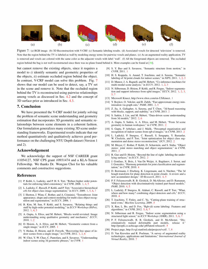
Figure 7: (a) RGB image. (b) 3D Reconstruction with V-CRF. (c) Semantic labeling results. (d) Associated voxels for detected ‘television’ is removed.Note that the region behind the TV is labeled as wall by modeling energy terms for pairwise voxels and planes. (e) As an augmented reality application, TVis removed and voxels are colored with the same color as the adjacent voxels with label ‘wall’. (f) All the foreground objects are removed. The occludedregion behind the bag is not well reconstructed since there was no plane found behind it. More examples can be found at [30].

but cannot remove the existing objects, since it requires amodel to i) identify semantic and geometric properties ofthe objects, ii) estimate occluded region behind the object.In contrast, V-CRF model can solve this problem. Fig. 7shows that our model can be used to detect, say, a TV setin the scene and remove it. Note that the occluded regionbehind the TV is reconstructed using pairwise relationshipsamong voxels as discussed in Sec. 4.2 and the concept of3D surface prior as introduced in Sec. 4.3.

7. ConclusionWe have presented the V-CRF model for jointly solving

the problem of semantic scene understanding and geometryestimation that incorporates 3D geometric and semantic re-lationships between scene elements in a coherent fashion.Our formulation generalizes many existing 3D scene under-standing frameworks. Experimental results indicate that ourmethod quantitatively and qualitatively achieves good per-formance on the challenging NYU Depth dataset (Version 1and 2).

AcknowledgementWe acknowledge the support of NSF CAREER grant

#1054127, NSF CPS grant #0931474 and a KLA-TencorFellowship. We thanks Dr. Wongun Choi for his valuablecomments and constructive suggestions.

References[1] P. Kohli, L. Ladicky, and P. H. S. Torr, “Robust higher order poten-

tials for enforcing label consistency,” in CVPR, 2008. 1, 4, 5[2] L. Ladicky, C. Russell, P. Kohli, and P. Torr, “Associative hierarchical

crfs for object class image segmentation,” in ICCV, 2009. 1, 5, 6, 7[3] J. Shotton, J. Winn, C. Rother, and A. Criminisi, “Textonboost: Joint

appearance, shape and context modeling for multi-class object recog-nition and segmentation,” in ECCV, 2006. 1

[4] B. Kim, M. Sun, P. Kohli, and S. Savarese, “Relating things andstuff by high-order potential modeling,” in ECCV Workshop (HiPot),2012. 1, 4, 5

[5] A. Gupta, A. Efros, and M. Hebert, “Blocks world revisited: Imageunderstanding using qualitative geometry and mechanics,” ECCV,2010. 1, 2

[6] D. Hoiem, A. A. Efros, and M. Hebert, “Geometric context from asingle image,” in ICCV, 2005. 1

[7] V. Hedau, D. Hoiem, and D. Forsyth, “Recovering free space of in-door scenes from a single image,” in CVPR, 2012. 1, 2, 6

[8] W. Choi, Y.-W. Chao, C. Pantofaru, and S. Savarese, “Understandingindoor scenes using 3d geometric phrases,” in CVPR. 1

[9] S. Y. Bao and S. Savarese, “Semantic structure from motion,” inCVPR, 2011. 1

[10] H. S. Koppula, A. Anand, T. Joachims, and A. Saxena, “Semanticlabeling of 3d point clouds for indoor scenes,” in NIPS, 2011. 1, 2, 3

[11] D. Munoz, J. A. Bagnell, and M. Hebert, “Co-inference machines formulti-modal scene analysis,” in ECCV, 2012. 1, 2, 3

[12] N. Silberman, D. Hoiem, P. Kohli, and R. Fergus, “Indoor segmenta-tion and support inference from rgbd images,” ECCV, 2012. 1, 2, 3,5, 7

[13] Microsoft Kinect, http://www.xbox.com/en-US/kinect. 1[14] Y. Boykov, O. Veksler, and R. Zabih, “Fast approximate energy min-

imization via graph cuts,” PAMI, 2001. 2, 5[15] Z. Jia, A. Gallagher, A. Saxena, and T. Chen, “3d-based reasoning

with blocks, support, and stability,” in CVPR, 2013. 2[16] S. Satkin, J. Lin, and M. Hebert, “Data-driven scene understanding

from 3d models,” 2012. 2, 6[17] A. Gupta, S. Satkin, A. A. Efros, and M. Hebert, “From 3d scene

geometry to human workspace,” in CVPR, 2011. 2[18] S. Gupta, P. Arbelaez, and J. Malik, “Perceptual organization and

recognition of indoor scenes from rgb-d images,” in CVPR, 2013. 2[19] L. Ladicky, P. Sturgess, C. Russell, S. Sengupta, Y. Bastanlar,

W. Clocksin, and P. Torr, “Joint optimization for object class seg-mentation and dense stereo reconstruction,” IJCV, 2012. 2

[20] M. Bleyer, C. Rother, P. Kohli, D. Scharstein, and S. Sinha, “Objectstereo: joint stereo matching and object segmentation,” in CVPR,2011. 2

[21] R. Guo and D. Hoiem, “Beyond the line of sight: labeling the under-lying surfaces,” in ECCV, 2012. 2

[22] J. Gonfaus, X. Boix, J. Van De Weijer, A. Bagdanov, J. Serrat, andJ. Gonzalez, “Harmony potentials for joint classification and segmen-tation,” in CVPR, 2010. 4

[23] D. Borrmann, J. Elseberg, K. Lingemann, and A. Nuchter, “The 3dhough transform for plane detection in point clouds: A review and anew accumulator design,” 3D Research, 2011. 4, 5

[24] P. F. Felzenszwalb, R. B. Girshick, D. McAllester, and D. Ramanan,“Object detection with discriminatively trained part-based models,”PAMI, 2010. 4, 5

[25] L. Ladicky, P. Sturgess, K. Alahari, C. Russell, and P. Torr, “What,where and how many? combining object detectors and crfs,” ECCV,2010. 4

[26] T. Joachims, T. Finley, and C. Yu, “Cutting-plane training of struc-tural svms,” Machine Learning, 2009. 5

[27] X. Ren, L. Bo, and D. Fox, “Rgb-(d) scene labeling: Features andalgorithms,” in CVPR, 2012. 5, 6, 7

[28] N. Silberman and R. Fergus, “Indoor scene segmentation using astructured light sensor,” in ICCV Workshop (3DRR), 2011. 5, 6, 7

[29] P. F. Felzenszwalb, R. B. Girshick, and D. McAllester, “Dis-criminatively trained deformable part models, release 4.”http://people.cs.uchicago.edu/ pff/latent-release4/. 5

[30] Project page, http://cvgl.stanford.edu/projects/vcrf/. 7, 8[31] D. Van Krevelen and R. Poelman, “A survey of augmented reality

technologies, applications and limitations,” International Journal ofVirtual Reality, 2010. 7