development of calibrated operational models for real-time decision support and performance...
TRANSCRIPT

Development of Calibrated Operational Models for Real-Time Decision Support and Performance OptimisationDaniel Coakley BE PhD CEM MIEI MEI Research Fellow, Integrated Environmental Solutions Ltd.Adjunct Lecturer, National University of Ireland GalwaySecretary, ASHRAE Ireland
CIBSE Technical Symposium 2016, April 14-15, Heriot Watt Uni, Edinburgh

Structure• Introduction• Energy in Time Methodology
– Model Development, Performance Analysis & Calibration;– Control optimisation
• Case Study: Sanomatalo– Model development and calibration;– Sensitivity analysis;– Performance analysis (M&V);– Genetic optimisation;
• Conclusions– Calibration process summary;– Conclusions & Future work.

INTRODUCTION
Energy in Time Project
Model Development & Calibration
Control Optimisation

Company Background• Founded 1994 with HQ in
Glasgow;
• Offices worldwide;
• Focused on delivering sustainable solutions from building to city-scale;
• Main software:
– IES-VE (Building simulation)
– IES-ERGON (Building operations)
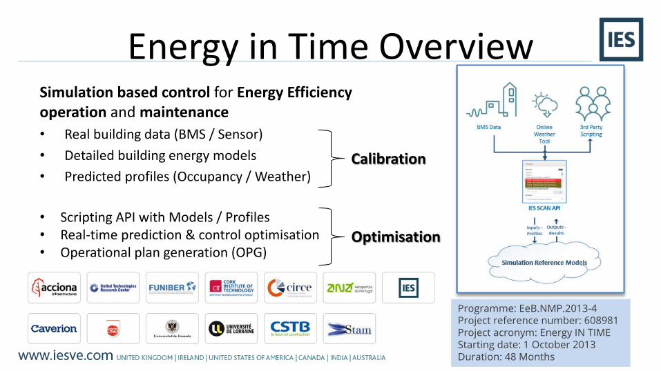
Energy in Time OverviewSimulation based control for Energy Efficiency operation and maintenance
• Real building data (BMS / Sensor)
• Detailed building energy models
• Predicted profiles (Occupancy / Weather)Calibration
• Scripting API with Models / Profiles• Real-time prediction & control optimisation• Operational plan generation (OPG)
Optimisation
Programme: EeB.NMP.2013-4Project reference number: 608981Project acronym: Energy IN TIMEStarting date: 1 October 2013Duration: 48 Months

Model Calibration Building energy models may be used in all phases of
BLC from design to commissioning and operation. However, for operational use, there is a need to address any discrepancies between design performance and actual performance;
Building Model Calibration is the process of improving the accuracy of simulation models to reflect the as-built status and actual operating conditions;
Calibration performance assessed using standard statistical indices:
𝑀𝐵𝐸 % =
𝑖=1
𝑁𝑝 𝑚𝑖 − 𝑠𝑖
𝑖=1
𝑁𝑝𝑚𝑖
𝐶𝑉 𝑅𝑀𝑆𝐸 % =
𝑖=1
𝑁𝑝 𝑚𝑖 − 𝑠𝑖2
𝑁𝑝
𝑚
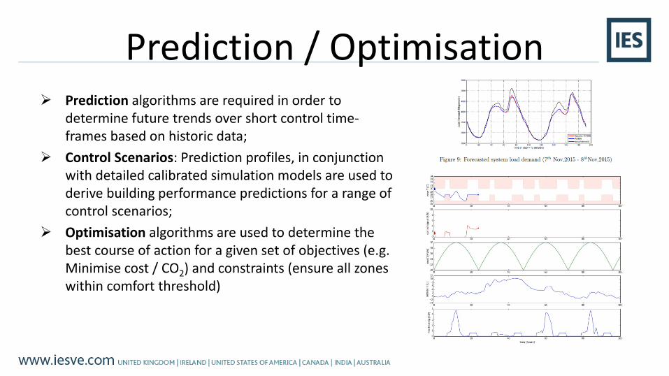
Prediction / Optimisation Prediction algorithms are required in order to
determine future trends over short control time-frames based on historic data;
Control Scenarios: Prediction profiles, in conjunction with detailed calibrated simulation models are used to derive building performance predictions for a range of control scenarios;
Optimisation algorithms are used to determine the best course of action for a given set of objectives (e.g. Minimise cost / CO2) and constraints (ensure all zones within comfort threshold)

METHODOLOGY
Overview
Model Development & Calibration
Control Optimisation
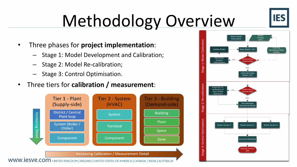
Methodology Overview• Three phases for project implementation:
– Stage 1: Model Development and Calibration;
– Stage 2: Model Re-calibration;
– Stage 3: Control Optimisation.
Static Model
Parameters
Model
Profiles
<FFP>
Building
Operational Data
<SCAN>
Base Model <VE>
Sensitivity
Analysis
<PB+Python>
Update Model
Performance
Criteria MetNO
Calibrated Base
Model <VE>
YES
Re-calibrated
Operational Model
Performance
Criteria Met?
YES
Automatic re-
calibration of
Input Profile
<Optimise>
NO
Model Variant 1 Model Variant 2 Model Variant 3
Scenario Modelling
Optimal Control
DSS
Model Variant 2
• Three tiers for calibration / measurement:
Static Model
Parameters
Model
Profiles
<FFP>
Building
Operational Data
<SCAN>
Base Model <VE>
Sensitivity
Analysis
<Python>
Update Model
Performance
Criteria MetNO
Calibrated Base
Model <VE>
YES
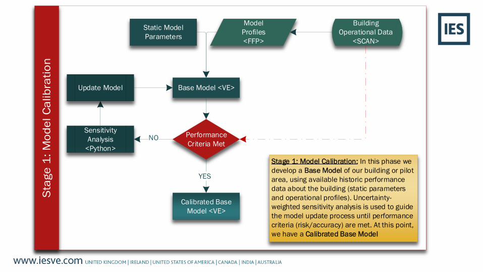
Stage 1: Model Calibration: In this phase we
develop a Base Model of our building or pilot
area, using available historic performance
data about the building (static parameters
and operational profiles). Uncertainty-
weighted sensitivity analysis is used to guide
the model update process until performance
criteria (risk/accuracy) are met. At this point,
we have a Calibrated Base Model

Calibrated Base
Model <VE>
Re-calibrated
Operational Model
Performance
Criteria Met?
YES
Automatic re-
calibration of
Input Profile
<Optimise>
NO
Stage 2: Model Re-calibration: As the model
will be used during building operation, it is
necessary to regularly assess performance
criteria and re-calibrate the model if
performance drift occurs. In this phase,
uncertain model profiles (e.g. occupancy,
infiltration) will be adjusted automatically
using an optimisation function. This is known
as the Calibrated Operational Model and may
be used to make reliable predictions for
ongoing building operation and control.

Re-calibrated
Operational Model
Model Variant 1
Stage 3: Control Optimisation: In this phase,
we introduce the concept of model variants,
which represent significant changes to the
calibrated base model (e.g. CV vs VAV). Each
model variant may be run on the Apache
cloud, under different scenarios (UGR). The
results of these model scenarios will provide
a control DSS for the building manager.
Model Variant 2 Model Variant 3
Scenario Modelling
Optimal Control
DSS

CASE STUDY: SANOMATALO
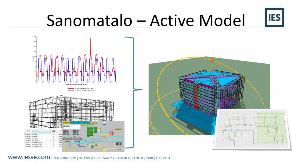
Sanomatalo – Active Model

Sensitivity Analysis
Normalised Sensitivity Index
Parameter
Total Energy [MWh]
Total System Energy [MWh]
Boilers Energy [MWh]
Chillers Energy [MWh]
Room Air [C]
Overall
AAHX_latent_effectivenss 0.002 0.002 0.001 0.003 0.000 0.001
AAHX_sensible_effectivenss 0.905 0.905 0.792 0.100 0.371 0.615
air_flow 1.000 1.000 0.060 0.116 0.079 0.451
conductivity_ceiling 0.055 0.055 0.076 0.085 0.080 0.070
cool_setpoint 0.000 0.000 0.000 0.000 0.000 0.000
equipment_gain 0.103 0.039 0.204 0.141 0.120 0.121
glazing_conductivity 0.057 0.057 0.151 0.047 0.117 0.086
glazing_transmittance 0.130 0.130 0.393 1.000 0.280 0.387
infiltration 0.315 0.315 0.893 0.230 0.461 0.443
lighting_gain 0.244 0.163 0.639 0.359 0.322 0.346
occupancy_gain 0.010 0.010 0.143 0.166 0.151 0.096
radiator_max_timestep 0.001 0.001 0.000 0.001 0.000 0.001
radiator_midband 0.568 0.568 0.720 0.317 1.000 0.635
radiator_panel_weight 0.003 0.003 0.000 0.003 0.000 0.002
radiator_radiant_fraction 0.008 0.008 0.010 0.011 0.003 0.008
radiator_water_capacity 0.003 0.003 0.001 0.005 0.000 0.003
steam_humidifier_humidity 0.003 0.003 0.000 0.008 0.000 0.003
supply_temp 0.587 0.587 1.000 0.315 0.515 0.601
Sensitivity analysis was carried with respect toparameter impact on five key model outputs:• Total energy [MWh]• Total System Energy [MWh]• Boilers Energy [MWh]• Chillers Energy [MWh]• Room Air Temperature [oC]

Measured and Simulated data were compared for the calibration period for the following output parameters:
Heating Coil Load (kW) - Hourly
Boiler Load (kW) – Hourly
CVRMSE NMBE
Sum of Diff ^2 2821.505 Sum of Diff 81.76972
No. Samples 409 n-p 408
Mean Observation 20.805 kW Mean Observation 20.805 kW
CVRMSE 12.624 % NMBE 0.963 %
Mean Bias Error (MBE) (%)
𝑀𝐵𝐸 % =
(𝑚𝑖 − 𝑠𝑖)𝑁𝑝
𝑖=1
(𝑚𝑖)𝑁𝑝
𝑖=1
Coefficient of Variation of Root Mean Square Error CV(RMSE) (%)
𝐶𝑉 𝑅𝑀𝑆𝐸 % =
(𝑚𝑖 − 𝑠𝑖)
2𝑁𝑝
𝑖=1
𝑁𝑝
𝑚
Performance Analysis
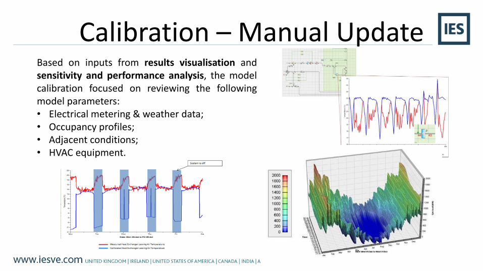
Calibration – Manual UpdateBased on inputs from results visualisation andsensitivity and performance analysis, the modelcalibration focused on reviewing the followingmodel parameters:• Electrical metering & weather data;• Occupancy profiles;• Adjacent conditions;• HVAC equipment.

Genetic OptimisationGenetic Optimisation is used to further refine the model by automatically modifying static input parameters and profiles.
generation = 114
objectives variables
NMBE CVRMSE supply_temp infiltration lighting_gain AAHX_sensible_effectivenssair_flow radiator_midband
0.00 20.55 1.49 0.89 1.10 45.71 0.92 22.90
0.00 20.53 1.45 0.77 0.92 43.98 0.94 22.81
0.00 20.48 1.46 0.88 0.72 45.69 0.92 22.88
0.01 20.46 1.47 0.91 0.84 45.57 0.90 22.88
0.02 20.45 1.48 0.78 1.01 44.52 0.96 22.82
0.02 20.45 1.48 0.78 0.65 44.52 0.96 22.82
0.04 20.45 1.50 0.77 1.31 43.94 0.94 22.82
0.04 20.45 1.50 0.77 0.95 43.94 0.94 22.82
0.04 20.45 1.50 0.77 0.95 43.94 0.94 22.82
0.04 20.45 1.50 0.77 1.27 43.94 0.94 22.82
0.05 20.42 1.49 0.87 0.51 45.83 0.94 22.88
0.05 20.37 1.47 0.89 0.51 45.71 0.92 22.88
0.09 20.36 1.45 0.85 0.51 45.59 0.94 22.88
0.09 20.36 1.45 0.85 0.58 45.59 0.94 22.88
0.18 20.36 1.46 0.86 0.51 45.66 0.94 22.88
0.19 20.34 1.45 0.91 0.51 45.59 0.92 22.88
0.30 20.32 1.47 0.90 0.51 45.66 0.94 22.88
0.32 20.31 1.45 0.91 0.51 45.59 0.92 22.88
0.56 20.28 1.50 1.08 0.68 44.85 0.85 22.88
0.56 20.28 1.50 1.08 0.56 44.85 0.85 22.88
0.56 20.28 1.50 1.08 0.67 44.85 0.85 22.88
0.59 20.27 1.48 1.05 0.81 44.95 0.86 22.88
0.60 20.24 1.50 1.05 0.77 44.85 0.86 22.88
0.67 20.20 1.49 1.05 0.56 44.95 0.86 22.88
0.95 20.20 1.49 1.11 0.55 44.85 0.86 22.88
0.95 20.19 1.50 1.00 1.04 45.65 0.94 22.89
1.01 20.18 1.49 1.11 0.62 44.85 0.86 22.88
1.01 20.18 1.49 1.11 0.62 44.85 0.86 22.88
1.24 20.17 1.45 1.04 0.91 45.63 0.93 22.93
1.24 20.17 1.45 1.04 0.60 45.63 0.93 22.93
1.28 20.17 1.43 1.02 1.07 45.60 0.93 22.93
1.28 20.17 1.43 1.02 1.02 45.60 0.93 22.93
1.28 20.17 1.43 1.02 1.15 45.60 0.93 22.93
1.36 20.15 1.46 1.11 1.03 46.61 0.95 22.93
1.46 20.15 1.47 1.11 0.83 45.83 0.95 22.85
1.51 20.09 1.45 1.11 0.67 46.35 0.95 22.93
1.68 20.07 1.45 1.12 0.83 45.85 0.94 22.93
1.70 20.07 1.45 1.11 0.83 45.85 0.95 22.93
1.80 20.05 1.48 1.16 0.57 45.71 0.93 22.91
1.88 20.00 1.50 1.19 0.60 46.51 0.94 22.91
2.26 19.97 1.50 1.24 0.75 46.66 0.96 22.91
2.37 19.95 1.50 1.26 0.58 46.62 0.95 22.91
2.73 19.93 1.49 1.31 0.95 46.62 0.96 22.91
2.97 19.92 1.50 1.36 0.85 46.62 0.96 22.91
2.97 19.92 1.50 1.36 0.84 46.62 0.96 22.91
range: 0.07 0.59 0.81 2.72 0.11 0.11
average: 1.48 1.01 0.77 45.43 0.92 22.89
range/average: 0.05 0.59 1.04 0.06 0.12 0.00
count: 45
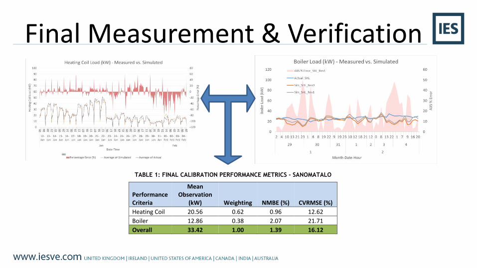
Final Measurement & Verification
TABLE 1: FINAL CALIBRATION PERFORMANCE METRICS - SANOMATALO
Performance Criteria
Mean Observation
(kW) Weighting NMBE (%) CVRMSE (%)
Heating Coil 20.56 0.62 0.96 12.62
Boiler 12.86 0.38 2.07 21.71
Overall 33.42 1.00 1.39 16.12

CONCLUSIONS
Calibration process summary
Conclusions
Future Work
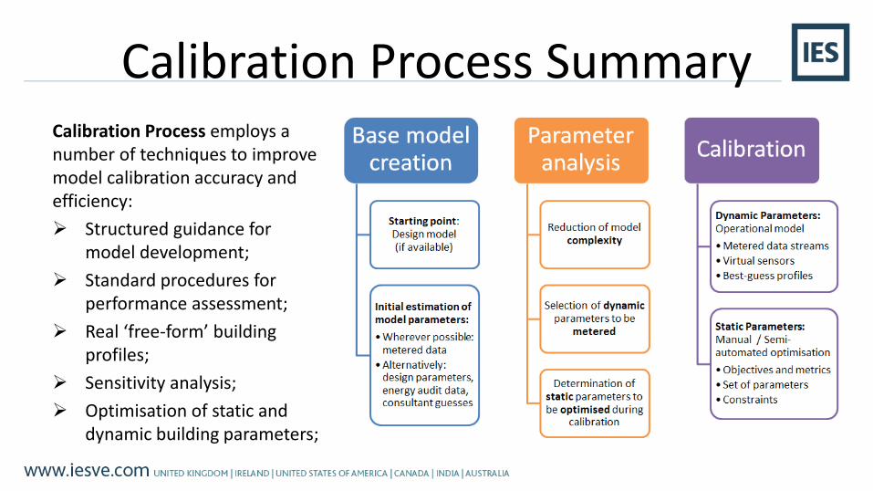
Calibration Process SummaryCalibration Process employs a number of techniques to improve model calibration accuracy and efficiency:
Structured guidance for model development;
Standard procedures for performance assessment;
Real ‘free-form’ building profiles;
Sensitivity analysis;
Optimisation of static and dynamic building parameters;
Conclusions• There are many tools and methods available to aid model development and calibration – lack
of clear guidance on calibration requirements and standards;
• Hybrid method combines real building data with model physics to provide more accurate simulation with reduced time to implementation. When used appropriately, may offer an excellent alternative to full simulation models;
• Statistical and graphical analysis provides a means of structuring model development, and assigning time and resources more effectively (e.g. Sensitivity, Uncertainty and Performance analysis);
• Optimisation methods provide a robust means of refining parameter estimates. Need to be used with caution to avoid ‘tuning’ parameters incorrectly;
• Access to a real building performance repository could help improve profile estimation and predictions;

Future Work• Complete testing of approach for four EU sites:
– Test Site 1: Airport in Faro, Portugal
– Test Site 2: Office and Test Labs in Bucharest, Romania
– Test Site 3: Commercial and Office in Helsinki, Finland
– Test Site 4: Hotel in Levi-Lapland, Finland
• Integrate cloud simulation models with real building data streams for automated model performance analysis and re-calibration (where required);
• Test and deploy operational plan generator (OPG) on pilot sites;

Thank you!
Daniel Coakley BE PhD CEM MIEI MEI Research Fellow, Integrated Environmental Solutions Ltd.Adjunct Lecturer, National University of Ireland GalwaySecretary, ASHRAE IrelandEmail: [email protected]: www.iesve.com
CIBSE Technical Symposium 2016, April 14-15, Heriot Watt Uni, Edinburgh