Development of a Parallel SAR Processor on a

Beowulf Cluster

Thomas Gerald Hart Bennett

A dissertation submitted to the Department of Electrical

Engineering,

University of Cape Town, in fulfilment of the requirements

for the degree of Master of Science in Engineering.

Cape Town, December 2003

Declaration

I declare that this dissertation is my own, unaided work. It is being submitted for

the degree of Master of Science in Engineering in the University of Cape Town. It

has not been submitted before for any degree or examination in any other university.

Signature of Author . . . . . . . . . . . . . . . . . . . . . . . . . . . . . . . . . . . . . . . . . . . . . . . . . . . . . . . . . . . . . .

Cape Town

February 2003

i

Abstract

The purpose of this dissertation is to present the development and testing of the

parallelisation of a Range-Doppler SAR processor. The inherent data parallelism

found in SAR data lead to the choice of using master slave parallel processor, where

copies of a slave task perform the same tasks on different sets of data. However,

the SAR processor that was parallelised needed to implement a corner turn without

saving data to disk keeping the data set being processed distributed in memory over

the nodes in the cluster. This was successfully achieved using a in-place method, thus

saving valuable memory resources. Once the parallel processor was implemented

some timing tests where performed, yeilding a maximum speedup factor of 6.2 for

an 8 slave processor system.

ii

Dedication

This thesis is dedicated to all those who encoraged me to finish it.

iii

Acknowledgements

This thesis would not have been possible with out the financial support from the

CSIR DefenceTek who funded the second year of my Masters Program. I would also

like to thank Prof. Mike Inggs, Dr. Jasper Horrel, Mark Gerbhard and Dr. Richard

Lord for their assistance and guidance.

iv

Contents

Declaration i

Abstract ii

Acknowledgements iv

Nomenclature x

1 Introduction 1

1.1 Background to SAR . . . . . . . . . . . . . . . . . . . . . . . . . . . . 1

1.2 Background to Beowulf Clusters . . . . . . . . . . . . . . . . . . . . . 2

1.3 SASAR background[14] . . . . . . . . . . . . . . . . . . . . . . . . . . 3

1.4 Objectives . . . . . . . . . . . . . . . . . . . . . . . . . . . . . . . . . 3

1.5 Plan of Development . . . . . . . . . . . . . . . . . . . . . . . . . . . 4

2 Principals of SAR 5

2.1 Introduction . . . . . . . . . . . . . . . . . . . . . . . . . . . . . . . . 5

2.2 Geometry and Terminology for Strip-Mapped SAR . . . . . . . . . . 5

2.3 Range Processing . . . . . . . . . . . . . . . . . . . . . . . . . . . . . 6

2.3.1 Pulse Compression . . . . . . . . . . . . . . . . . . . . . . . . 7

2.3.2 Motion Compensation . . . . . . . . . . . . . . . . . . . . . . 8

2.3.3 Interference Suppression . . . . . . . . . . . . . . . . . . . . . 9

2.4 Azimuth Processing . . . . . . . . . . . . . . . . . . . . . . . . . . . . 10

2.4.1 Azimuth Processing Algorithm . . . . . . . . . . . . . . . . . 11

v

2.4.2 Range Curvature Correction . . . . . . . . . . . . . . . . . . . 11

3 Principles of Parallel Computing 12

3.1 Introduction . . . . . . . . . . . . . . . . . . . . . . . . . . . . . . . . 12

3.2 Taxonomy of Parallel Computers . . . . . . . . . . . . . . . . . . . . 12

3.3 Messaging Middle-ware . . . . . . . . . . . . . . . . . . . . . . . . . . 15

3.3.1 Message Passing Implementations . . . . . . . . . . . . . . . . 15

3.3.2 Parallel Virtual Machine . . . . . . . . . . . . . . . . . . . . . 15

3.4 Parallel Processing Theory . . . . . . . . . . . . . . . . . . . . . . . . 17

3.4.1 Amdahl’s Law . . . . . . . . . . . . . . . . . . . . . . . . . . . 17

3.4.2 Processor Speedup Factor . . . . . . . . . . . . . . . . . . . . 17

4 Parallel Processor Implementation 19

4.1 Introduction . . . . . . . . . . . . . . . . . . . . . . . . . . . . . . . . 19

4.2 Processor Source Code . . . . . . . . . . . . . . . . . . . . . . . . . . 20

4.3 Implementation of the Master Process . . . . . . . . . . . . . . . . . 20

4.3.1 Initialisation Phase . . . . . . . . . . . . . . . . . . . . . . . . 20

4.3.2 Starting up the Slave Processes . . . . . . . . . . . . . . . . . 23

4.3.3 Scatter the Raw Data to the Slave Processes . . . . . . . . . . 24

4.3.4 Receiving Processed Data from Slave Processes . . . . . . . . 24

4.4 Implementation of the Slave Process . . . . . . . . . . . . . . . . . . 25

4.4.1 Initialisation Phase . . . . . . . . . . . . . . . . . . . . . . . . 25

4.4.2 Range Compression Implementation . . . . . . . . . . . . . . . 26

4.4.3 Corner Turn Implementation . . . . . . . . . . . . . . . . . . . 26

4.4.4 Azimuth Compression Implementation . . . . . . . . . . . . . 26

4.5 Corner Turn Implementation . . . . . . . . . . . . . . . . . . . . . . . 27

4.5.1 In-place Matrix Transpose . . . . . . . . . . . . . . . . . . . . 29

4.5.2 Message Passing Phase Implementation . . . . . . . . . . . . . 29

4.6 Conclusion . . . . . . . . . . . . . . . . . . . . . . . . . . . . . . . . . 30

vi

5 Analysis and Results 32

5.1 Data Set . . . . . . . . . . . . . . . . . . . . . . . . . . . . . . . . . . 32

5.2 Comparison of Serial to Parallel Version . . . . . . . . . . . . . . . . 32

5.2.1 Performance Comparison . . . . . . . . . . . . . . . . . . . . . 32

5.2.2 Image Output Comparison . . . . . . . . . . . . . . . . . . . . 33

5.3 Timing Output Analysis . . . . . . . . . . . . . . . . . . . . . . . . . 33

5.4 Tracking of Memory Usage . . . . . . . . . . . . . . . . . . . . . . . . 35

5.5 Conclusion . . . . . . . . . . . . . . . . . . . . . . . . . . . . . . . . . 36

6 Conclusions and Future Work 37

A Setup file template 38

Bibliography 44

vii

List of Figures

2.1 SAR Geometry . . . . . . . . . . . . . . . . . . . . . . . . . . . . . . 6

3.1 CISE Taxonomy (taken from CISE web page) . . . . . . . . . . . . . 13

4.1 G2 parallel processor program flow . . . . . . . . . . . . . . . . . . . 21

4.2 Program Data Flow . . . . . . . . . . . . . . . . . . . . . . . . . . . . 22

4.3 Distributed Matrix Transpose . . . . . . . . . . . . . . . . . . . . . . 28

viii

List of Tables

2.1 Notch Filter Parameters . . . . . . . . . . . . . . . . . . . . . . . . . 10

2.2 LMS Filter Parameters . . . . . . . . . . . . . . . . . . . . . . . . . . 10

3.1 Comparison of Message Passing Implementations[9] . . . . . . . . . . 15

4.1 Example of parameters sent in multi-cast message . . . . . . . . . . . 24

4.2 Setup values for Corner Turn Configuration . . . . . . . . . . . . . . 30

5.1 Critical Processor Parameters . . . . . . . . . . . . . . . . . . . . . . 32

5.2 Processor Comparison . . . . . . . . . . . . . . . . . . . . . . . . . . 33

5.3 Changing number of slave processes with constant image size size . . 35

5.4 Changing image size, using constant number of slaves processes . . . 35

ix

Nomenclature

Azimuth — Angle in a horizontal plane, relative to a fixed reference, usually north

or the longitudinal reference axis of the aircraft or satellite.

Beamwidth — The angular width of a slice through the mainlobe of the radiation

pattern of an antenna in the horizontal, vertical or other plane.

Cluster of Workstations (COW) — Workstations that are connected together

via a hub or a switch.

Doppler frequency — A shift in the radio frequency of the return from a target

or other object as a result of the object’s radial motion relative to the radar.

Distributed Corner Turn — Corner turn implementation done using multiple

compute nodes.

Message Middleware — A common communications interface between software

applications in a generic parallel system.

Message Passing Implementation (MPI) — Messaging middle-ware imple-

mentation.

Range—The radial distance from a radar to a target.

Real Apperture Radar (RAR) — Standard method for side looking airborne

radar, where the azimuth resolution is limited by the physical length of the radar

appeture.

Synthetic Aperture Radar (SAR) — A signal-processing technique for improv-

ing the azimuth resolution beyond the beamwidth of the physical antenna actually

used in the radar system. This is done by synthesizing the equivalent of a very long

sidelooking array antenna.

Swath — The area on earth covered by the antenna signal.

Parallel Virtual Machine (PVM) — Messaging middle-ware implementation.

x

Chapter 1

Introduction

1.1 Background to SAR

Synthetic aperture radar (SAR) 1 is a microwave technique, capable of producing

high-resolution images by synthesising a the equivalent of a long side-looking array

antenna. A fully processed SAR image is a photograph-like representation of the

band-limited microwave reflectivity of the Earth’s surface.

SAR has become an invaluable remote sensing technique, due to its advantage over

optical and infrared imaging techniques. This is because SAR is an active microwave

technique, and therefore not dependent on illumination from the sun or radiation

from Earth. Since SAR uses electro-magnetic waves having a lower frequency than

light, they can penetrate cloud cover and see through rain with a limited attenuation

to the received signal, thus allowing day/night all-weather imaging.

Given the above reasons, SAR has been implemented for many commercial as well

as military applications. Commercial applications include topographic mapping,

mining, geology[18], time difference images that can be used in vegetation discrim-

ination, rate of urbanisation and oil pollution monitoring[13]. In the military sphere,

SAR can be used for tactical reconnaissance, which has the advantage at Very High

Frequency (VHF) band of locating targets hidden under foliage due to the long wave

length of the transmitted pulse[10].

SAR is, however, characterised by high data rates and requires comprehensive com-

putations to process the raw data into a focused image. Since its inception in 1967[4],

there has always been a need for faster processing speeds to the point where the SAR

processing can be done in real time. Many contemporary solutions involve paral-

lel processing, which improves the throughput by taking advantage of the inherent

parallel nature of SAR processing.

1For a thorough overview of SAR the reader is referred to [4].

1

Parallel processing is a dynamic field, and the next section introduces the back-

ground to parallel processing and the type of parallel processor used in this disser-

tation.

1.2 Background to Beowulf Clusters

Parallel processing is an umbrella term used to describe a set of processors working

together to find the solution to a given problem. Parallel processors appear in many

forms, and the hardware ranges from traditional massively parallel processors to a

peer-to-peer connection over the Internet.

The use of massively parallel processors such as the Cray T3 and the Intel Big

Blue has been limited to projects with big budgets, as they are extremely expensive

machines to purchase and maintain. Once the purchased the user is also linked into

proprietary software written for a specific machine and is therefore reliant on the

manufacturer for software upgrades and hardware improvements.

However, in recent years, the increasing processing power of modern desktop PC’s

and the decrease in cost of off-the-shelf networking technologies has made the idea

of a cluster of workstations a viable approach for running parallel applications on

scalable and versatile parallel processors. Coupled with the use of open source

software these technologies lead to the most famous fast cluster of workstations

being constructed in 1994 at the NASA Goddard Centre [1]. This cluster consisted

of 16 DX4 processors connected by channel-bonded Ethernet and was called Beowulf.

Inspired by this, all other parallel processors of a similar anatomy have since been

called Beowulf clusters. Although originally only consisting of a small number of

nodes, as in the Goddard Cluster, there are now Beowulf clusters that consist of

hundreds of nodes.

The Radar Remote Sensing Groups (RRSG) Beowulf Cluster is called Gollach [[11]],

and was used as a hardware benchmark for this dissertation. This system is designed

for the development and testing of parallel implementations. The current system is

configured to run code developed using Parallel Virtual Machine (PVM) and Mes-

sage Passing Interface (MPI). The system also runs Mosix, a Linux kernel module

that enables the transparent migration of tasks. The cluster hardware specifications

are:

• 1 Dual-CPU Intel Pentium II, 350 MHz machine, 512 M Bytes RAM;

• 7 Single-CPU Intel Pentium II 350 MHz machines, 256 M Bytes RAM;

• a CISCO CS2912 12-port Fast Ether-Net Switch

2

The next section gives a brief overview of the RRSG’s SAR processor and the

RADAR hardware used to collect raw data for processing.

1.3 SASAR background[14]

The South African Synthetic Aperture Radar (SASAR) is an airborne SAR system

developed by the RRSG at UCT and the Defencetek division of the Council for Sci-

entific and Industrial Research (CSIR - Defencetek). Although originally designed

to be installed on a Boeing 707 aircraft, the experimental radar was installed on a

South African Air-force DC3 (Dakota) aircraft. Work began on the system in 1993,

but due to budget cuts, the system first flew in January of 1999. Since then a series

of flights have been performed, the last being in January 2000.

The SASAR system operates in the VHF band at 141 MHz and has a 12 MHz

bandwidth. The antenna consists of four inclined monopoles mounted on the right,

rear side of the fuselage. A pulse expander has been developed to increasing the

on-target energy and is capable of transmitting pulses of up to 15 µs in length.

The signal processing for SASAR data is performed with the G2 post-processor

developed by Horrel [12], which uses a range-Doppler approach to focus the data.

The next section covers the objectives for this dissertation.

1.4 Objectives

The objective of this dissertation is to implement and test a parallel version of the G2

processor using a Beowulf Cluster. This dissertation is based on an implementation

of independent work done at the University of Cape Town.

The original code for the G2 processor was written in C, and the parallel version is

an adaptation of the existing C code. The parallel processor must take advantage

of the inherent parallelism of SAR processing, so that the data can be split into

sections and processed independently. The processor must also implement a corner

turn, which must keep all the data in fast access RAM memory distributed across

the processors.

Once the G2 processor has been mapped to a parallel version, it has to be shown

that the parallel processor successfully focus SAR images. Finally the processor

needs to be analysed in terms of parallel processor performance metrics.

3

1.5 Plan of Development

The remainder of this dissertation is structured in the following manner:

Chapter 2 covers the fundamentals of SAR processing and relevant mathematical

equations. This chapter also introduces relevant theory for specific aspects a

SAR data processor. These aspects include airborne SAR geometry, motion

compensation and interference suppression.

Chapter 3 covers parallel processing fundamentals. A taxonomy for parallel pro-

cessors is given. A discussion on messaging middle-ware is then given with

an overview of Parallel Virtual Machine. Performance metrics such as pro-

cessor speed-up, memory use and a comparison between the parallel and serial

version that will be used to asses the parallel processors are also discussed.

Chapter 4 describes the implementation of the design theory to map the SAR

processing to a parallel version. A description of the master and slave pro-

cesses is given. One of the aspect of this chapter is the implementation of the

distributed matrix corner turn.

Chapter 5 displays the results and analysis of the parallel processor. Firstly the

parallel processor is compared with the current serial processor. Then the

output of the processor is analysed, and some timing results are given.

Chapter 6 gives the conclusions and recommendations are made for future work

on the parallel processor.

Appendix A is the template file of the process configuration file.

4

Chapter 2

Principals of SAR

2.1 Introduction

This section covers some of the basic theory needed to understand an airborne range-

Doppler VHF SAR processor and more specifically SASAR the SAR platform that

was used to record actual data, and the G2 parallel processor.

A critical issue in SAR imaging is resolution, and in the sections that follow it is

shown how high range resolution can be achieved by conditioning the data and using

by coded pulses. High azimuth resolution can also be achieved by synthesising a

long antenna with a relatively small antenna structure. Firstly, a brief description

of the geometry and terminology is needed.

2.2 Geometry and Terminology for Strip-Mapped

SAR

The oldest mode of SAR operation, is strip-mapped SAR, it is still the most widely

used to date and best describes the processor implementation used in this disser-

tation. Figure 2.1 shows a diagram of the geometry for strip-mapped SAR. From

this figure it can be seen that the antenna array is fixed into position on the fusel-

age of the aircraft, mounted at an elevated look angle. The antenna emits pulses

at a constant Pulse Repetition Interval (PRI), which illuminate the ground and is

scattered in all directions, including the direction of the antenna. The radar foot-

print represents the intersection of a transmitted electro-magnetic pulse with the

Earth’s surface. The range extent of the footprint is known as the ground swath.

The width of the footprint is determined by the azimuth beam width of the antenna

at a given range.

5

Look Angle

Nadir Track

Flight Path

Swath Width

Antenna Footprint

Figure 2.1: SAR Geometry

Many pulses are transmitted in the time it takes the aircraft to travel the width of

the footprint, so that each target in the ground swath is illuminated many times over

as the radar passes by. As is often the case with imaging techniques, it is desirable

to achieve a high resolution. The next section deals with how high range resolution

can be achieved.

2.3 Range Processing

Range processing in this dissertation is the term used to describe the algorithms that

are implemented by the SAR processor on the received data in a range direction.

This multi-functional task may include factors such as pulse compression, motion

compensation and interference suppression, depending on what is needed to achieve

the optimum range resolution and from the received raw data and optimising the

focused data using other recorded data such as the motion of the aircraft platform.

Range resolution is the measurement of the extent to which a target can be discrim-

inated from other targets in its vicinity. Since modern SAR systems rely on digital

recording techniques, range resolution is also related to the processed image pixels,

and a simple relationship between the two can be found. The range pixel spacing,

∆r, is given in Equation 2.1, where fsampleis the A/D sample rate. The ground

range pixel spacing, ∆r, is given in Equation 2.2, where θ is the look angle.

6

∆r =c

2fsample

(2.1)

∆g =∆r

sin(θ)(2.2)

From a radar design perspective, range resolution is dependent on specific properties

of the transmitted pulse that is used by the radar. The simplest form that a trans-

mitted pulse can take is a monochromatic pulse. The resolution that is achievable

by a monochromatic pulse can be shown to be related to the inverse of the spatial

extent (or the 3dB bandwidth) of the signal, as shown in Equation 2.3 . Therefore,

in order to obtain a high range resolution, a signal with a short spatial extent is

needed.

ρ =cτ

2(2.3)

Radars are limited by the transmit peak of their power amplifiers. This ceiling

on the transmitter strength, limits the maximum achievable range resolution using

this type of pulse, as sorter pulses require high peak transmit power to ensure an

acceptable Signal to Noise Ratio (SNR) for the received signal.

However, buy using pulse coding methods, longer pulses can be transmitted giving

sufficient energy in returned signals and high bandwidth can still be achieved.

2.3.1 Pulse Compression

Pulse compression is a common signal processing technique that can be used to

increase the range resolution of transmitted pulse without having to increase the

peak transmit power.

One particular type of coded pulse used is linear frequency modulation or the linear

chirp, which has been implemented by Horrel and is used in this dissertation. In

this form of pulse compression the transmitted signal is modulated with a linearly

varying frequency. The modulated form of the chirp pulse is shown in Equation 2.4.

sRF (t) = cos

[

2π

(

fot + Kt2

2

)]

|t| ≤τ

2(2.4)

Here, SRF is the time domain description of a signal where fo is the carrier centre

frequency and the pulse duration is defined by |t| ≤ τ2. A characteristic of the chirp

waveform coding technique is the dispersion factor (or time-bandwidth product)

7

D = K t2

2[16].

After convolving the received signal with a time reversed representation of the trans-

mitted pulse, a high range resolution is obtained when compared to a monochromatic

pulse of similar length. The bandwidth that is achievable using this technique is

stated in Equation 2.5, where it shows that the bandwidth of the received pulse is

β.

β = Kτp (2.5)

One of the disadvantages of this pulse is that the main lobe to side lobe ratio is

approximately -13dB, but this can be improved by weighting the wave form with a

window function before compression[20].

There are other aspects of the SAR processor that optimise the final processed SAR

images: namely motion compensation and interference suppression. These are dealt

with in the next sub-sections.

2.3.2 Motion Compensation

This sub-section is an overview of motion compensation and how it is implemented

in SASAR and the G2 parallel post processor.1

Motion compensation is an integral part of SAR processing, as motion errors cause

distortions in the processed image. In azimuth processing, phase information is im-

portant and needs to be accurate within a fraction of a wavelength to be acceptable.

The ideal flight path is a parallel to the imaging swath. However this is never

achievable, due to atmospheric turbulence, high altitude winds and navigation er-

rors. Three dimensional accelerometers or Inertial Measurement Unit (IMU) and

Global Positioning Satellite (GPS) position data is recorded on the SASAR plat-

form used for post processing. Data correction for motion compensation in the G2

parallel processor is broken down into three steps:

1. Accurate reconstruction of the flight path from IMU and GPS data.

2. Interpolating and matching a point in the flight path to each transmitted pulse.

3. Implementation of corrections using the reconstructed flight path.2

As in most strip-mapped SAR implementations, the strategy employed for motion

compensation by the G2 processor is to correct the data to a nominal straight flight

path. This nominal flight path can be defined as a straight line between the starting

1For a more details see [12], Chapter 5.2Only this step is implemented in this dissertation.

8

point of data capture to the end point of data capture, taking the average altitude

of the aircraft between the two points.

The flight deviation from the nominal flight path, results in the processor performing

a range shift of ∆R and a phase shift of ∆ϕ on each range line of data, given in

Equation 2.6.

∆ϕ =4π

λ∆R (2.6)

Motion compensation is performed after range compression in the G2 parallel pro-

cessor. It consists of a range shift by 8 point Shannon interpolation, and a phase

shift implemented as a complex multiply to each range line.

It is noted that the motion compensation has a limitation in that the correction is

only exact for some reference range, which is usually chosen to be in the middle of the

range swath. For VHF radar, the synthetic aperture length is very large compared

to higher frequency SAR systems, so this approach for motion compensation is only

approximate, but works if the aircraft motion is not too extensive.

2.3.3 Interference Suppression

There are many commercial services such as television broadcasting, mobile com-

munications and cellular phones that transmit in the VHF band, which form inter-

ference patterns in the processed image. One way to get rid of the RFI is to increase

the radars transmitted signal, but it then might interfere with the commercial trans-

missions. In Lord, R Aspects of Stepped-Frequency Processing for Low-Frequency

SAR Systems [17] the RFI has been characterised as narrow band compared to the

radar transmitted signal and is fairly constant over a number (up to 5000) of range

lines.3

Notch Filter

A notch filter is a frequency domain implementation to remove the RFI, and tapers

off spikes in a range line’s magnitude spectrum. Since the signal is random in nature,

by taking an average of a number of magnitude range spectra and the RFI being

fairly constant will be enhanced and notches can be added to the matched filter.

For the G2 parallel processor, the notch update rate does not necessarily have to be

the same length as the number of Fast Fourier Transform (FFT) lines used to find

3Although there are many different ways of suppressing RFI, only two are described here, asthey are part of the G2 processor and implemented by Lord. [17]

9

Table 2.1: Notch Filter Parameters

Processor Parameter Default Value

Notch update rate 100Number of FFT Lines used for FFT 100

Notch cutoff 3 dBMedian kernel length 33

Table 2.2: LMS Filter Parameters

G2 Parameter Default Value

LMS update rate 10LMS number of weights 512

LMS side lobe order 0

the notches. It is also possible to set the notch cutoff value, expressed in decibels.

The kernel length for the median filter to find the spikes can also be set. The typical

values for SASAR are given in Table 2.1 showing the notch filter parameters.4

LMS adaptive filter

As its name suggests it is an adaptive filter using a Least Mean Square (LMS)

algorithm that can track time variations in the statistics of the input data.5

For the G2 processor, the LMS update rate can be set so it uses the same filter over

a number of lines. The LMS number of weights can be set as well as the side lobe

order. With reference to Table 2.2, typical parameters for SASAR data are shown.

2.4 Azimuth Processing

What separates SAR processing from other radar techniques is the way that high

azimuth resolution is achieved.

For conventional Real Aperture Radar (RAR), azimuth resolution depends on the

real length of the antenna Areal and is approximated in Equation 2.7 where λ is the

wavelength, and R is the slant range to the target.

δreal ≈Rλ

Areal

(2.7)

4For more detail on the Notch Filter see [17]Chapter 4.55For more detail on the LMS adaptive filter see [17] Chapter 4.6

10

This physical limitation on array size for airborne radars means it is difficult to

achieve high azimuth resolution for RAR.

However, using SAR processing techniques it can be shown that the azimuth resolu-

tion is dependent on the length of the synthesised aperture, which is stated directly

in Equation 2.8. Note that this is the small azimuth beam width approximation.

δsar ≈λR

2L(2.8)

The value for L in equation 2.8, is the length of the synthetic aperture and it is

only limited by a target needing to be in the real beam width of the radar, thus the

wider the beam-width the higher azimuth resolution that can be achieved.

2.4.1 Azimuth Processing Algorithm

There is a strong correlation between the chirp pulse and the algorithm that is used

for azimuth compression. The mathematics can be derived from the geometry and

after making some approximations.6

2.4.2 Range Curvature Correction

As the range from radar to the target increases, the range curvature increases and

may extend over multiple range bins. This excessive range curvature can cause

the energy from a target to be spread over multiple range bins that are not in the

same range line. In order to align the received energy from a particular target,

range curvature needs to be calculated and the data needs to be corrected. This is

achieved using interpolation for sub-pixel accuracy and the data is shifted. Range

curvature is most often a problem for low frequency SAR as the reference functions

are long compared to higher frequency radars.

6For a detailed description of azimuth processing the reader is referred to [19]

11

Chapter 3

Principles of Parallel Computing

3.1 Introduction

There are many suitable candidates for parallelisation that have been proposed

and implemented over the years, including complex system models, simulations and

’grand challenge’ problems[2]. This chapter provides a description of parallel com-

puters and where the parallel processor used in this dissertation falls into the of

parallel processor family tree. It describes some of the fundamental concepts, the-

ories and software implementations that form a background to this dissertation.

3.2 Taxonomy of Parallel Computers

There are many variations on the parallel theme, which are often differentiated or

taxonomised in terms of their hardware profile and implementation software lib-

raries. The first widely accepted taxonomy for parallel computers was devised by

Flynn in 1966, which is still in use today. He categorised all computer architectures

according to the number of instruction streams and data streams:

• Single instruction single data (SISD): A sequential computer like the von Neu-

mann model used in modern PC’s.

• Single instruction multiple data (SIMD): A style of processors that work on

vectors of data (used in Graphics chips)

• Multiple instruction multiple data (MIMD): This is defined as many processors

simultaneously executing different instructions on different data.

• Multiple instruction single data (MISD): No well known systems are docu-

mented.

12

Parallel computers

MIMDSIMD

Shared Memory Distributed Memory

DSM LinearSMP NUMA Fixed Scalable

Figure 3.1: CISE Taxonomy (taken from CISE web page)

Despite the popularity of Flynn’s taxonomy, his system does have inherent problems

as MISD is not widely implemented. In light of these problems, new taxonomies

have expanded on Flynn’s original system. One such system has been set up by the

University of Florida CISE department.

This new taxonomy is taken from the consensus that the areas that have seen the

most growth need further subdivision. Figure 3.1 shows the additions that have

been made to Flynn’s system by University of Florida’s CISE department[23].

From Figure 3.1 it can be seen that for SIMD no further definition refinement was

given. However, MIMD systems have been split further according to the memory

organisation, namely shared memory and distributed memory. These two categories

have also been further subdivided, and there are six classifications according to the

CISE taxonomy:

• Symmetric multiprocessing (SMP): Here, the memory is shared, and all pro-

cessors access the memory equally at equal speeds.

• Non-uniform memory access (NUMA): For this implementation, the memory

is physically shared but not distributed on an equal basis amongst the pro-

cessors.

• Distributed Shared Memory (DSM): Here, the memory is distributed amongst

the processors, but it appears contiguous at the application level.

• Fixed : Here, the number of connections is fixed. An example is a Cluster of

Workstation (COW) connected via a hub or switch, as hubs and switches can

only handle a pre-allocated number of processors.

• Linear : Here, the number of connections grows linearly with the number of

nodes. An example is mesh connected multicomputers such as the Intel Par-

agon.

13

• Scalable: the number of connections grows as P × log(P ) or greater with the

number of nodes. An example is hypercubes such as the Intel iPSC/860.

It would possible to add more branches to the CISE taxonomy, but according to

CISE there is no clear consensus about what these categories should be. For the pur-

poses of this dissertation the CISE taxonomy is a good enough description. However

other taxonomies do exist using different aspects of parallel processors to differenti-

ate them.

Over the past few decades COWs have become a cost efficient option over the more

expensive super computers like Crays. This is because COWs consist of a hetero-

geneous cluster of workstations, which can be used as individual workstations or

working together in cluster. New nodes are off-the-shelf commodities and can be

added dynamically to the network with very little implementation overhead. COWs

are also no longer locked into reliance on proprietary software vendors allowing op-

erating systems and other software to be modified and updated with at the fraction

of the cost of the hardware maintenance of the system.1

The parallel processor used as the bench mark in this dissertation is a Beowulf

Cluster which falls under the COWs section of the CISE taxonomy. Beowulf Clusters

are so named after the first of its kind which was developed at NASA’s Jet Propulsion

Laboratory and was called Beowulf.

A more formal definition of Beowulf Cluster, is a high performance computing cluster

that has some or all of the following components:

• Using Commercial Off the Shelf (COTS) hardware (such as PC’s, switches

and hubs)

• Using one of the many flavours of message middle-ware, including the following

products:

– Parallel Virtual Machine (PVM)

– Message Passing Interface (MPI)

– MOSIX

Beowulf clustering has a low cost for performance due to COTS hardware and low

risk due to source software. This has made Beowulf clustering a viable solution,

compared to the other parallel processing hardware solutions.

1For a thorough overview of the state of Parallel Processing the reader is referred to [27]

14

Table 3.1: Comparison of Message Passing Implementations[9]Option PVM BNM

Spawn method User daemon System daemonStartup command pvm bnmrunSpawn command pvm spawn

UDP communication default NoUDP packet size 4K (settable w/ pvm setop) N/A

TCP communication PvmRoutDirect(pvm setop) defaultTCP packet size 4K (settable w/ pvm setop) maximum

Option LAM MPICH

Spawn method User daemon System, user or rsh daemonStartup command mpirun mpirunSpawn command MPI Spawn() N/A

UDP communication default NoUDP packet size 8K N/A

TCP communication -c2c (mpirun option) defaultTCP packet size maximum maximum

3.3 Messaging Middle-ware

Middle-ware, or more specifically messaging middle-ware, is the software layer that

can best be described as a common communications interface between software

applications in a generic parallel system. This allows tasks - either on local or

remote machines to send data back and forth to each other in a synchronous or

asynchronous manner. Data sent to a particular program is stored in a queue and

then forwarded to the receiving program when the receiving task becomes available

to process it. There are many message passing implementations that have been

developed. The next two sub-sections illustrates a few of these implementations.

3.3.1 Message Passing Implementations

Two of that have been used on the Beowulf Cluster at UCT are Parallel Virtual

Machine (PVM) and the Message Passing Interface (MPI) standard implementa-

tion called MPICH. Since PVM was used for the parallel implementation for this

dissertation the next sub-section gives an overview of PVM.2

3.3.2 Parallel Virtual Machine

Parallel Virtual Machine (PVM) collaborated venture between Oakridge National

Laboratory , the University of Tennessee, Emory University and Caregie Mellon

2For a comparison between the PVM and MPI and other standards see [9].

15

University[9]. It is a popular parallel system implementation that can be used to

view a large number of heterogeneous hosts in a network or ever across the Internet

as a single available resource. It is based around the concept of a virtual machine

that consists of two parts: the PVM daemon and a set of PVM library routines that

can be called from a PVM task.

The PVM daemon run on each node in the network and is responsible for spawning

tasks, performing inter-task communications and data distribution.

PVM provides routines for packing and sending data between tasks, transmitting

messages over the underlying network hardware using appropriate protocols, such

as Unix Datagram Protocol (UDP) or Transfer Control Protocol (TCP).The library

routines are available for may common programming languages: C, FORTRAN,

Java and Python.

There is a command line interface for PVM that can be used to start the PVM

daemon and add hosts to the PVM configuration. There is a graphic front end called

XPVM which provides task trace output and other useful graphic information.

PVM Maintenance Routines

pvm spawn() is used to spawn other tasks in the PVM environment. pvm getop

and pvm setop() are used to get and set the PVM environment options. Some of

these options include PvmRouteDirect which routes messages directly to receiving

tasks.

pvm joingroup() is used to initialise and maintain process groups. By using the

function pvm barrier() call all tasks in a group need to have made a similar call

before tasks can continue.

PVM Message Passing and Packing Routines

PVM send routines are nonblocking pvm send(), while PVM receive routines can

be either blocking pvm recv() or non-blocking pvm nrecv(). The same message

can be sent to multiple tasks by using pvm mcast() call.

Data is sent and received through message buffers. Data typing is maintained by

packing it into a send buffer. It is left up to the receiving task to unpack the data

according to the format in which it was packed. pvm pk*() is used to pack data

and pvm upk*() is used to unpack data in order.

16

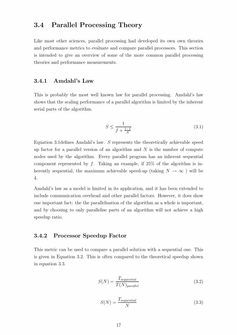
3.4 Parallel Processing Theory

Like most other sciences, parallel processing had developed its own own theories

and performance metrics to evaluate and compare parallel processors. This section

is intended to give an overview of some of the more common parallel processing

theories and performance measurements.

3.4.1 Amdahl’s Law

This is probably the most well known law for parallel processing. Amdahl’s law

shows that the scaling performance of a parallel algorithm is limited by the inherent

serial parts of the algorithm.

S ≤1

f + 1−f

N

(3.1)

Equation 3.1defines Amdahl’s law. S represents the theoretically achievable speed

up factor for a parallel version of an algorithm and N is the number of compute

nodes used by the algorithm. Every parallel program has an inherent sequential

component represented by f . Taking an example, if 25% of the algorithm is in-

herently sequential, the maximum achievable speed-up (taking N → ∞ ) will be

4.

Amdahl’s law as a model is limited in its application, and it has been extended to

include communication overhead and other parallel factors. However, it does show

one important fact: the the parallelisation of the algorithm as a whole is important,

and by choosing to only parallelise parts of an algorithm will not achieve a high

speedup ratio.

3.4.2 Processor Speedup Factor

This metric can be used to compare a parallel solution with a sequential one. This

is given in Equation 3.2. This is often compared to the theoretical speedup shown

in equation 3.3.

S(N) =Tsequential

T (N)parallel

(3.2)

S(N) =Tsequential

N(3.3)

17

However, it is generally noted that as a rule of thumb the theoretical speedup usually

has an efficiency around 60%, and Equation 3.3 can be modified accordingly, as is

shown in Equation 3.4.

S(N) =Tsequential

0.6N(3.4)

18

Chapter 4

Parallel Processor Implementation

4.1 Introduction

As has been indicated there already exists a serial version of a SAR processor know

as the G2 processor. This chapter describes in detail the parallel version of the G2

processor which was derived from the serial version.

The G2 parallel processor can be best described as a data parallel processor, taking

advantage of the fact that, a small subset of range lines can be processed independ-

ently from the rest of the image in a range direction and a small subset of azimuth

lines can be processed independently of the rest of the image in an azimuth direction.

However, there is a limit to how many range lines or azimuth lines can be processed

independently. This is due to the fact that range presuming is implemented to in-

crease the SNR of the received signal and the RFI suppression notch filter needs a

number of range lines to create its filter. In the azimuth direction, range curvature

correction requires a number of azimuth lines for interpolating the range curve to

a sub-pixel level. Since range compression and azimuth compression are independ-

ent processes, the processor implements a range compression algorithm (with data

conditioning capabilities), a corner turn and an azimuth compression algorithm.

The G2 parallel processor is divided up as a master task and a group of slave tasks.

The parallel processor is fully scalable from 2 to N slave tasks. Since the hardware

bench mark for the G2 parallel processor is an 8 node Beowulf cluster there is no

point in implementing more than 8 slave tasks, as it hits a performance degradation

once the processor goes beyond the 1 processor 1 task threshold. It is better to have

1 process handling a large set of data than two processes handling smaller sets of

data while they are competing for CPU time. The master task is spawned on a dual

Pentium processor so a slave can be spawned on the same node as the master task,

with minimal effect on the loading to that node.

19

4.2 Processor Source Code

The processor source codes can be found on the attached compact disk in the dir-

ectory */thesis source/.

Source code Contents

Pg2Mrnc.c Master process source code

Pg2Srnc.c Slave process source code

g2000.jcc Code Crusader (jcc) project header file

*.c & *.h All other source code and header files for functions and procedures

Makefile.aimk Special PVM make file

The next sections deals with the implementation of the master process.

4.3 Implementation of the Master Process

The master-slave model is a standard approach that can be used to implement

parallel programs. This model divides the responsibilities neatly between a master

process that is in control of data flow and the processing environment and the slave

tasks which performing the algorithms that need to be implemented on the data set.

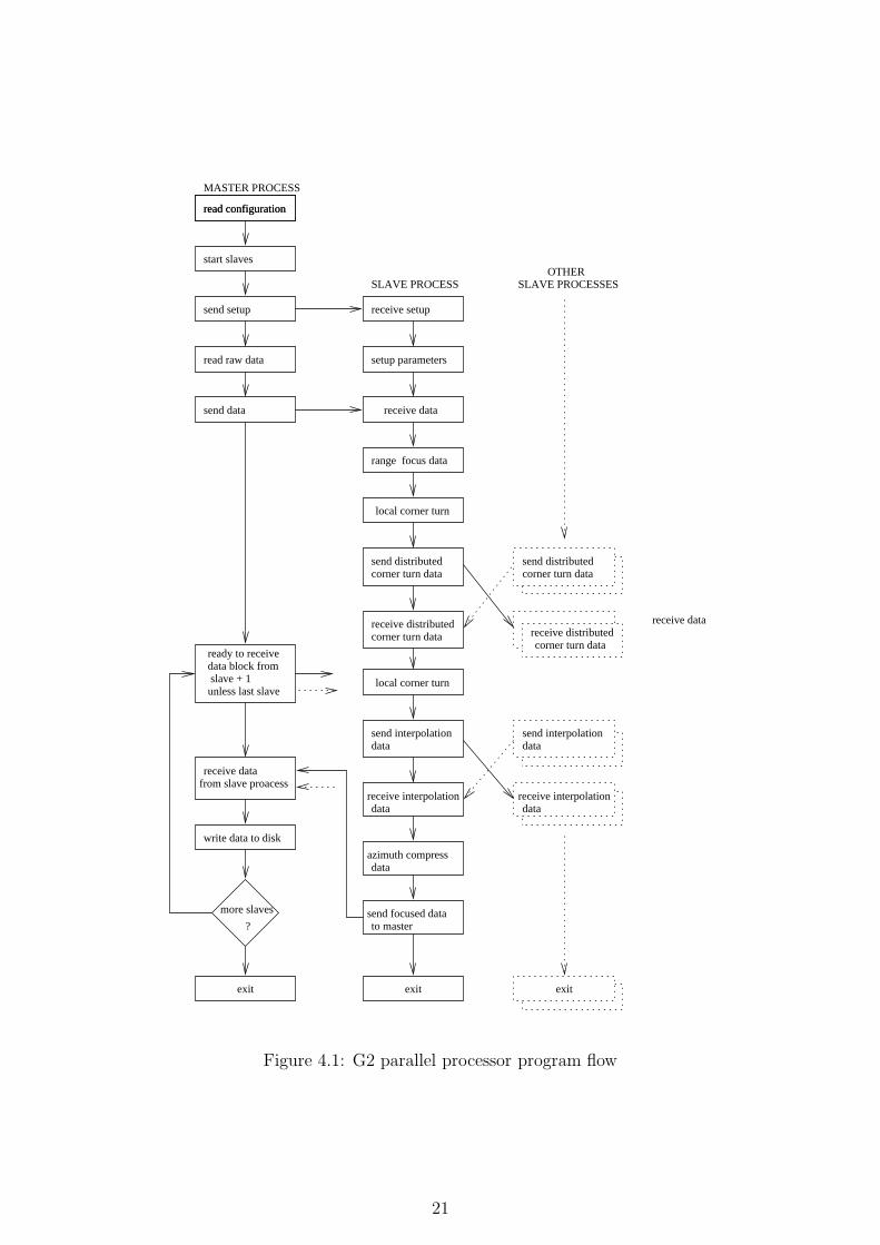
4.3.1 Initialisation Phase

The first step for the master process is to read in data from the setup file that follows

as a command line argument when the master processes is started. This setup file is

indicated in Figure 4.2 as ’general setup file’. During this phase some error checking

is performed to make sure that there are no conflicting setup parameters. This step

does not require any interaction with the PVM environment.

Next the master process initialises the PVM environment and spawns the slave

processes. It is assumed that the PVM daemon has been started up prior to

the master task being started. In order to optimise the message overhead the

pvm setopt(PvmRoute, 3) option is set, routing messages directly to tasks. The

master process will then attempt to spawn a slave task on a node in the cluster

that has the least number of PVM tasks running on it. Thus if there are 8 available

nodes in the cluster and 8 slaves need to be spawned, the master process will spawn

seven slaves on their own nodes and spawn the last slave on the same node as the

master process, assuming that the master process was spawned on the first node in

cluster processor list. The master tasks uses the information made available by the

20

read configurationread configuration

send setup

start slaves

read raw data

send data

setup parameters

range focus data

local corner turn

send distributedcorner turn data

send interpolationdata

local corner turn

dataazimuth compress

send focused datato master

exit exit

more slaves

?

write data to disk

receive setup

MASTER PROCESS

SLAVE PROCESSES

receive datafrom slave proacess

OTHERSLAVE PROCESS

send interpolationdata

corner turn data

receive interpolationdata

exit

send distributed

receive data

corner turn datareceive distributedcorner turn data

receive distributed

receive data

receive interpolationdata

ready to receive data block from slave + 1unless last slave

Figure 4.1: G2 parallel processor program flow

21

master task

pvm_mcast

read from file

read from file

read from file

(ASCII text)

(ASCII text)

compensation

pvm_send

raw data

(ASCII text)DistributedCorner turn

(ASCII text)

Step Freq

STC data

General setup

file

write to fileprocessed data

setup data

read from fileread from file

read from file

pvm_recv

pvm_send pvm_recv

pvm_recv

data

Input

filemotion

data

file

file

Setupfile

Setupfile

fileData

Output

taskslave

Figure 4.2: Program Data Flow

22

pvm config() function which returns a structure describing the PVM environment.

The master process checks the PVM tasks load only, i.e. it does not check the overall

load on each node, it checks through the PVM configuration function.

After the slaves have been spawned the master process sets up the parameters for

how to divide the data that needs to be processed between the slave tasks. If notch

filtering is being used for RFI suppression, a data overlap might be needed for the

notch filter to operate correctly and the size of this overlap is calculated, adding

extra range lines of data, so that at least a multiple N data lines exist at the end of

the data block for use by the filter, where N is the number of range lines needed to

calculate the notch filter.

Next, pointers to output files (i.e. for the processed data) are allocated and all other

processing setup data that is need from files is read into appropriate memory buffers.

This includes the motion compensation data, step frequency processing setup data,

STC data and the distributed corner turn setup data. All these are indicated in the

data flow diagram Figure 4.2.

In the original G2-processor software, in order to save memory the motion compens-

ation data is read from a file into a memory buffer only when required. The master

task, however reads motion compensation data into a buffer so that it can be sent to

the slave tasks. All motion compensation data is passed to all the slave processors.

But each slave is given a list of offsets so that it knows where to start applying the

motion compensation data to its raw data set.

Data read in from the setup files is used to calculate other processing parameters,

the most important of these being the frequency domain representation of the range

reference function for the match filter. The processor uses power of 2 FFT, so the

memory buffer size can be pre-calculated. The disadvantage is that it might use

large amounts of memory to produce an FFT representation of the range reference

function which is zero padded.

4.3.2 Starting up the Slave Processes

At this stage of the process all the parameters that the master task can define for the

problem have been calculated and all the slave tasks have been spawned, the setup

information now needs to be transfered to the slave processes. The initialisation

data and raw data have been divided into two separate message passing phases.

This is done because it takes time for the spawned slave processes to set themselves

up using the setup information and the master is can start reading in data from the

file while the slave tasks are processing the setup data. The setup data is multi-cast

to all the slaves as there is a lot of overlap data that each slave needs. Thus the

23

Table 4.1: Example of parameters sent in multi-cast message

Parameter Explanation

NumberOfSlaves Number of slaves used in processorTIDs Array of Slave Task ID’s

SizeToRead Size of input buffer to createFlg.RngCom Flow control flag for range compressionFlg.CnrTrn Flow control flag for corner turning

Flg.AzmCom Flow control flag for azimuth compression

PVM multi-cast option can taken advantage of for sending the setup information to

the slave processes. Firstly the information needs to be packed using the pvm pk*

functions and then using the PVM multi-cast function to send the data to all the

slave processes.1 The call looks like this in the code:

pvm mcast(TIDs, NumberOfSlaves, RNC SETUP)

TIDs is the PVM identity numbers for the slave processes and RNC SETUP is a

tag that is used to as a message identifier. Table 4.1 gives an example of some of

the parameters that are passed in the multi-cast message.

4.3.3 Scatter the Raw Data to the Slave Processes

The next phase is to pass the data that needs to be processed to the slave processes.

The data is passed as byte format to the slave processes, but they are capable of

processing ’unsigned char’ or ’float’ format data - by casting the data type once the

raw data has been received. It may be the case that the data is padded at the front

and end of each range line. This padding is passed to the slave processes, so that

block reads can be done from the hard disk. The slave process while processing

the data casts the data type and removes the header and footer information. The

input data is usually of byte type (SASAR input data is of type signed char) and

after being cast to floats they will be four times the original size of the input buffer,

depending on how much pre-summing is done on the input data. The processor is

capable of handing the input data in a float format but in this situation advantage

of the data representation is lost.

4.3.4 Receiving Processed Data from Slave Processes

Once the raw data has been sent to the slave processes, the master task idles until

the data has been processed by the slave tasks and has been sent back to the master

1For a full list of all the available pvm functions see the appropriate PVM documentation

24

process to save to disk. In the PVM model, message queues are stored in memory

on the receiving tasks machine, so it is important that slave tasks only send data

to the master task when memory space becomes available, otherwise the processor

running the master task will eventually have to swap the receiver buffer to disk,

greatly increasing the time it takes to save the data to file on disk. Thus the slave

tasks first waits for a request from the master task to send its data. While slave

N − 1’s data is being written to disk, slave N sends its data to the master process.

Once all the data has written to disk, the master task exits from the PVM environ-

ment and frees the resources it was using.

4.4 Implementation of the Slave Process

Each node in the cluster keeps a local copy of the executable for the slave task. So

when the master task spawns a slave task on a particular node, the executable does

not need to be sent to the designated processor to start execution, the local copy is

loaded into memory. Once a slave has been spawned it has its own unique TID tag,

and can have data sent to it by specifying this tag in a PVM message parameter.

4.4.1 Initialisation Phase

Once the slave task has been spawned by the master process, the slave needs to find

its unique TID value and the master processes TID value. These are necessary in

order to receive data from and send data to the master task. Once enrolled in the

PVM environment a work group is set up, using the pvm joingroup() function.

The first slave process that enters the group will create it automatically. The work

group facility is used to aid co-ordinate the distributed corner turn. Once again the

pvm setopt(PvmRoute, 3) is used to optimise the message overhead by passing

data directly to tasks, i.e. not via the PVM daemon.

The slave process is responsible for processing the data it receives from the master

according to the rules and information it has been sent via the setup message from

the master task. Depending on what has been requested, the slave process is capable

of performing motion compensation, two flavours of RFI suppression (not at the

same time), range compression, a distributed corner turn and azimuth compression.

This functionality was done to maintain the general processor capability of the G2

processor, as well as assist in debugging. By setting values for specified flags it is

possible to toggle these functions according to what is required.

25

4.4.2 Range Compression Implementation

If the range compression flag has been set, range compression will be performed on

the input data. However, usually before the match filter algorithm is implemented

various data conditioning can be done on the data. This includes motion compens-

ation and RFI suppression. It is also possible to perform a simple pre-sum on the

data to increase the SNR. In order to save on memory, the output data is written

over the input data buffer. If the corner turn flag and azimuth compression flag

are not set, the slave task will send the data range compressed data to the master

process to save to disk.

4.4.3 Corner Turn Implementation

If the corner turn flag is set, the slave tasks will collaborate to perform a corner turn.

The slave tasks perform the corner turn independently from the master process. The

implementation of the corner turn is dealt with in more detail in a later section. If the

azimuth processing flag is not set the slave processes will perform the corner turn and

pass the data back to to the master process. It is thus possible to perform a corner

turn on a data set without performing range compression or azimuth compression.

4.4.4 Azimuth Compression Implementation

If the azimuth compression flag is set, the slave tasks will perform azimuth compres-

sion on the raw data set. Before the azimuth compression is performed extrapolation

data for the first and last lines of azimuth data needed is sent from one slave to the

other. When performing azimuth compression, the algorithm needs to have up to 8

range lines to determine the sub-pixel position of range curved range line. Once the

overlaps have been received azimuth compression can be done on the data. To save

memory the output data is written over the input data. Each slave processor will

calculate the parameters for azimuth compression according to its ’local’ near range

and far range values for its particular piece of the data set. This has implications on

the size of the match filter buffer that is allocated in memory for each slave and the

size of the FFT power of 2 buffer. By using the ’local’ near and far ranges instead of

the ’global’ values, the lower order slaves are able to use smaller power of 2 FFT’s.

The next section deals with the corner turn implementation of the G2 parallel pro-

cessor.

26

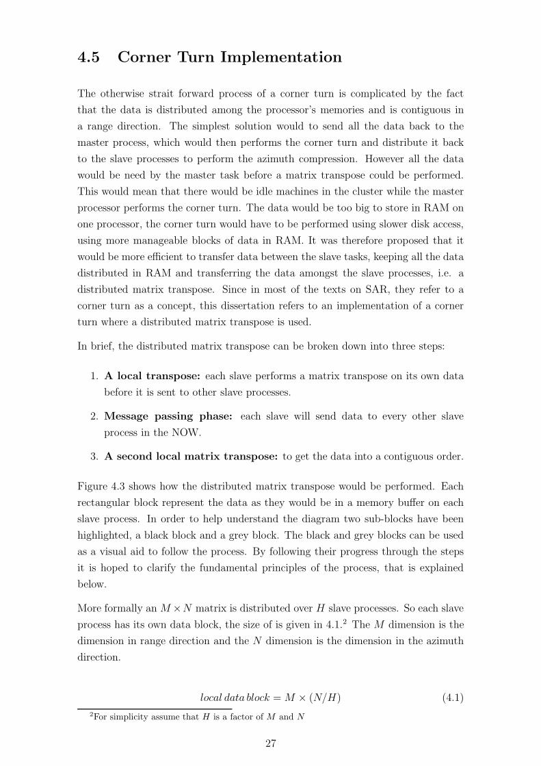
4.5 Corner Turn Implementation

The otherwise strait forward process of a corner turn is complicated by the fact

that the data is distributed among the processor’s memories and is contiguous in

a range direction. The simplest solution would to send all the data back to the

master process, which would then performs the corner turn and distribute it back

to the slave processes to perform the azimuth compression. However all the data

would be need by the master task before a matrix transpose could be performed.

This would mean that there would be idle machines in the cluster while the master

processor performs the corner turn. The data would be too big to store in RAM on

one processor, the corner turn would have to be performed using slower disk access,

using more manageable blocks of data in RAM. It was therefore proposed that it

would be more efficient to transfer data between the slave tasks, keeping all the data

distributed in RAM and transferring the data amongst the slave processes, i.e. a

distributed matrix transpose. Since in most of the texts on SAR, they refer to a

corner turn as a concept, this dissertation refers to an implementation of a corner

turn where a distributed matrix transpose is used.

In brief, the distributed matrix transpose can be broken down into three steps:

1. A local transpose: each slave performs a matrix transpose on its own data

before it is sent to other slave processes.

2. Message passing phase: each slave will send data to every other slave

process in the NOW.

3. A second local matrix transpose: to get the data into a contiguous order.

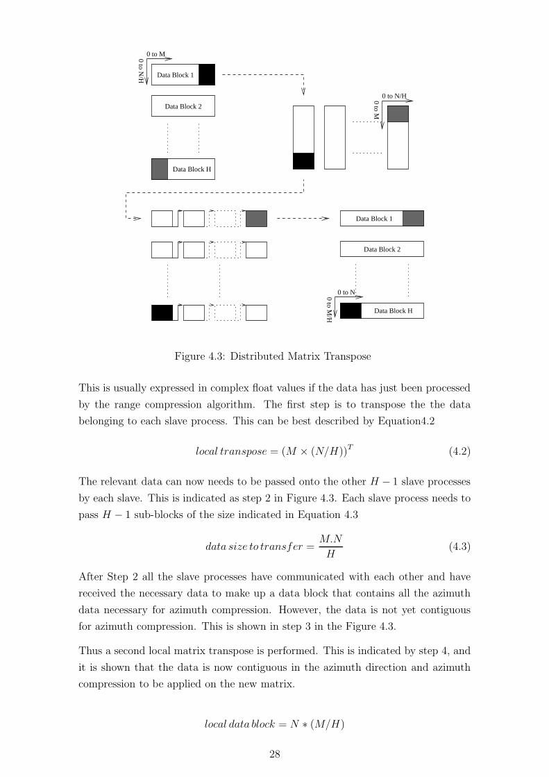
Figure 4.3 shows how the distributed matrix transpose would be performed. Each

rectangular block represent the data as they would be in a memory buffer on each

slave process. In order to help understand the diagram two sub-blocks have been

highlighted, a black block and a grey block. The black and grey blocks can be used

as a visual aid to follow the process. By following their progress through the steps

it is hoped to clarify the fundamental principles of the process, that is explained

below.

More formally an M ×N matrix is distributed over H slave processes. So each slave

process has its own data block, the size of is given in 4.1.2 The M dimension is the

dimension in range direction and the N dimension is the dimension in the azimuth

direction.

local data block = M × (N/H) (4.1)

2For simplicity assume that H is a factor of M and N

27

Data Block H

Data Block 2

Data Block 1

Data Block 1

Data Block 2

Data Block H

0 to M/H

0 to N/H0 to M

0 to M0 to N/H

0 to N

Figure 4.3: Distributed Matrix Transpose

This is usually expressed in complex float values if the data has just been processed

by the range compression algorithm. The first step is to transpose the the data

belonging to each slave process. This can be best described by Equation4.2

local transpose = (M × (N/H))T (4.2)

The relevant data can now needs to be passed onto the other H − 1 slave processes

by each slave. This is indicated as step 2 in Figure 4.3. Each slave process needs to

pass H − 1 sub-blocks of the size indicated in Equation 4.3

data size to transfer =M.N

H(4.3)

After Step 2 all the slave processes have communicated with each other and have

received the necessary data to make up a data block that contains all the azimuth

data necessary for azimuth compression. However, the data is not yet contiguous

for azimuth compression. This is shown in step 3 in the Figure 4.3.

Thus a second local matrix transpose is performed. This is indicated by step 4, and

it is shown that the data is now contiguous in the azimuth direction and azimuth

compression to be applied on the new matrix.

local data block = N ∗ (M/H)

28

This shows the basic overview of the distributed matrix transpose. The actual

implementation was taken from this design. The next sub-section deals with the

refinement of the local matrix transposes by doing them in-place.

4.5.1 In-place Matrix Transpose

The standard method used to transpose a matrix is to use a double buffer. Since

the processor will be dealing with large data sets the processor must processes as

much data as it can on each node of the NOW, an in-place matrix transpose was

investigated in order to maximise the data block size on each slave process.

This method uses reverse cyclic permutations.3 Circular permutations are used to

transpose the matrix in step 1 and step 3 indicated in Figure 4.3. By using an in-

place matrix transpose, larger amounts of RAM memory is available to store input

data sets at the cost of time to transpose the matrix and the is a penalty of overhead

of storing permutations that are used in the transpose.

Protnoff [22] proposes a special implementation of the in-place matrix called the

“Divide and Conquer Method”. For the implementation for this dissertation, the

cache hits did not not improve the performance much compared to the Cate and

Twigg method, however it worked just as well, so it was still used.4

4.5.2 Message Passing Phase Implementation

The message passing phase is a general purpose implementation. Since this is ac-

tually a matrix transpose the idea of circular permutations is used to perform the

message passing phase - step 3 in Figure 4.3.

The process is divided into rounds. Each round has a partner to pass data between.

This takes advantage of the Full Duplex Switched Ethernet available on the cluster.

In this mode the system each node is able to transmit and receive data simultan-

eously. Using a switched rather than shared connection to the hub, each node has the

possibility of sending and receiving 10Mb/s, for a theoretical aggregate of 20Mb/s

total, with the actual efficiency much lower. This actually eliminates the ”collision

detection” part of the Ethernet protocol.5

As an example to illustrate the data passing phase, the matrix below gives a de-

scription of four slave processes wishing to redistribute the distributed data set.

Each element has an x and y coordinate. The x coordinate describes who the data

3A permutation is a sequence of rules used to reorder a set of elements.[22]4For an example on reverse circular permutation see the example given [22]5Reference taken from http://www2.shore.net/˜jeffc/fdse/]

29

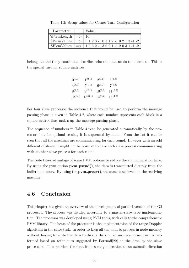
Table 4.2: Setup values for Corner Turn Configuration

Parameter Value

$PermLength => 16$PermValues => 0 1 2 3 -1 0 3 1 2 -1 0 2 1 3 -1 -2$ElemValues => 1 0 3 2 -1 3 0 2 1 -1 2 0 3 1 -1 -2

belongs to and the y coordinate describes who the data needs to be sent to. This is

the special case for square matrices

0(0,0) 1(0,1) 2(0,2) 3(0,3)

4(1,0) 5(1,1) 6(1,2) 7(1,3)

8(2,0) 9(2,1) 10(2,2) 11(2,3)

12(3,0) 13(3,1) 14(3,2) 15(3,3)

For four slave processor the sequence that would be used to perform the message

passing phase is given in Table 4.2, where each number represents each block in a

square matrix that makes up the message passing phase.

The sequence of numbers in Table 4.2can be generated automatically by the pro-

cessor, but for optimal results, it is sequenced by hand. From the list it can be

seen that all the machines are communicating for each round. However with an odd

different of slaves, it might not be possible to have each slave process communicating

with another slave process for each round.

The code takes advantage of some PVM options to reduce the communication time.

By using the pvm option pvm psend(), the data is transmitted directly from the

buffer in memory. By using the pvm precv(), the same is achieved on the receiving

machine.

4.6 Conclusion

This chapter has given an overview of the development of parallel version of the G2

processor. The process was divided according to a master-slave type implementa-

tion. The processor was developed using PVM tools, with calls to the comprehensive

PVM library. The heart of the processor is the implementation of the range-Doppler

algorithm in the slave task. In order to keep all the data to process in node memory

without having to write the data to disk, a distributed in-place corner turn is per-

formed based on techniques suggested by Portnoff[22] on the data by the slave

processors. This reorders the data from a range direction to an azimuth direction

30

in order for azimuth compression to be performed on SAR data.

31

Chapter 5

Analysis and Results

5.1 Data Set

The data set used to develop and test the G2 parallel processor was take from

SASAR flights over the Hermanus region, near Cape Town South Africa. The actual

flight data was captured on the 29 November 1999, and is located in a file called

leg1-vh.raw .

5.2 Comparison of Serial to Parallel Version

5.2.1 Performance Comparison

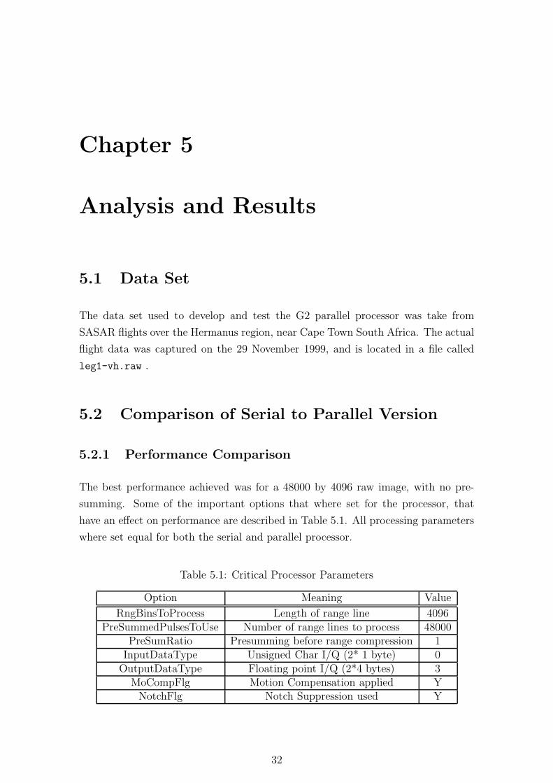
The best performance achieved was for a 48000 by 4096 raw image, with no pre-

summing. Some of the important options that where set for the processor, that

have an effect on performance are described in Table 5.1. All processing parameters

where set equal for both the serial and parallel processor.

Table 5.1: Critical Processor Parameters

Option Meaning Value

RngBinsToProcess Length of range line 4096PreSummedPulsesToUse Number of range lines to process 48000

PreSumRatio Presumming before range compression 1InputDataType Unsigned Char I/Q (2* 1 byte) 0

OutputDataType Floating point I/Q (2*4 bytes) 3MoCompFlg Motion Compensation applied Y

NotchFlg Notch Suppression used Y

32

Table 5.2: Processor Comparison

Processor Time(sec) Speedup

G2 processor 9344Theoretical Speedup 1168 8

Theoretical Speedup 60% Efficiency 1947 4.8G2 parallel processor - 8 slaves 1507 6.2

Table 5.2 shows the best performance for the most advantageous setup with respect

to the parallel processor. Here no pre-summing is done on the data - which means

that each slave performs range compression on its full data set, a factor which yields

the best speedup factor. If pre-summing is set so that less range compression is

performed on each slaves set of range lines, this reduces the speedup to 4.2, which is

below the industry rule of thumb of an efficiency of less than 60% when compared

to the serial version.

5.2.2 Image Output Comparison

The algorithms used for the serial and parallel versions are exactly the same, however

the focused images could differ due to differences in the way the azimuth compression

behaves. This is shown in section 4.4.4, and has to do with the size of the local FFT

buffer. By using the “local” far range to calculate the size of the FFT buffer the

lower order slaves are able to use smaller power of 2 FFT’s. This means that the

output will differ from the outputted image from the serial version.

The outputted images also differ when LMS filtering is implemented. The LMS filter

only settles down after the first processed range line, so the first line processed by

the LMS filter is not processed correctly. This can appear as while lines across the

image, and is the the first line that is the first line processed by each slave processor.

5.3 Timing Output Analysis

This section gives an analysis of the timing output of the G2 parallel processor. The

time to start and stop time is best described as the time from when the master task

starts to read the raw data from disk to when it writes the processed image to disk

after receiving it from the slave tasks. The time was measured using the functions in

the GNU C Library sys/time.h, which takes its timing from the system clock. The

appropriate Linux man page associated with sys/time.h, gives a timing resolution

of 10ms.

33

Below is an example of the time stamped output of the processor for a four slave

configuration (i.e. one master task and four slave tasks) with time stamping is given

in seconds. All these files can be found on the compact disk found attached to this

document in the directory

*/thesis tests/test[x]/test[x].output

where [x] is the selected tests. The listing below is sorted, gives the relevant inform-

ation and not the entire output.

Below is the master process output for test06:

------------

Prog: g2000 master (Ver. 1.0)

Copyright Radar Remote Sensing Group

Time To Read, Send - 10.150364 0.623390

Time To Read, Send - 10.046573 2.825272

Time To Read, Send - 10.044082 2.811263

Time To Read, Send - 10.044761 2.847841

R C A DONE - in 702.607383 secs.

The master process timing output shows the time to read the data from the disk

and the time take to send it to each slave process.

Below is the output for a slave process, the [t40003] is a PVM unique task identity

or TID. The size of the image processed in this example is a 16000 by 4066 image,

which is equally divided amongst the 4 slave processes (thus each slave process will

receive a 32 768 000 bit image to range compress). The value for actual size, shows

if there is padding added onto the received image, as padding is needed to simplify

the distributed corner turning process.

[t40003] BEGIN

[t40003] size = 32768000, actual size = 32768000

[t40003] 244.892360

[t40003] Starting DISTRIBUTED CORNER TURN

[t40003] C finished - in 62.032228 secs.

[t40003] FFT size: 16384 on 0

[t40003]A DONE before send - in 99.182076 secs.

[t40003] A DONE after send - in 3.377575 secs.

[t40003] EOF

Other values given, in the slave output is the time to perform the three stages of the

SAR processor (namely range compression, corner turn and azimuth compression).

The time it takes to send the data to the master process is also given.

34

Table 5.3: Changing number of slave processes with constant image size size

# of slaves processes Recorded timing results(sec) Performance comparison

2 4317.43 945.5 4.64 702.6 6.15 673.2 6.46 610.3 7.17 531.4 8.18 603.9 7.1

Table 5.4: Changing image size, using constant number of slaves processes

# of range lines processed Time to process image Performance comparison

16000 603.932000 1207.8 0.9342000 1585.2 1.0564000 2415.6 0.42

Table 5.3 shows the recorded results for processing a 16000 by 4096 image and

changing the number of slave processes between 2 and 8. Each slave is spawned on

its own node in the Gollach cluster. The third column shows the scaled improvement

i.e. how many times faster the process is than the two slave version. The biggest

improvement in speedup performance compared to the 2 slave version is for the 3

slave version. It is interesting to note that the 7 slave version has a better overall

timing result than the 8 slave version.

As the image size is increased, the performance of the processor - with all other

parameters held constant should scale linearly. However, due to the physical memory

limits of the processors, the is a point where the processor performance will start to

degrade. Table 5.4 shows the timing results when the image size is increased, while

keeping the number of slaves constant at 8. From the table it can be seen that the

performance of the processor has degraded as the image size is increased from 42000

range lines to 64000 range lines. The scaled performance is less than half for an

image four times bigger than the smallest size image size recorded.

5.4 Tracking of Memory Usage

The upper limit on the input image size is dependent on the memory size of each

processor, which in this case is 150 M Bytes of available memory. Once the im-

age gets to 48000 by 4096 (complex-float) the memory limits of the processors are

35

reached. After this size limit the processor starts page swapping the data as this

degrades performance, or the failure of a memory allocation malloc() command if

there is no more memory may crash the program.

5.5 Conclusion

This chapter describes the analysis of the G2 parallel processor. A comparison

is made with the original serial version of the G2 processor with the best speedup

result of 6.2 being achieved, the outputed images are also compared and the expected

differences are highlighted.

The parallel processor is also analysed by changing aspects of the parallel processor.

This included, firstly increasing the number of slave processes which compute a same

size image and secondly, increasing the image size while keeping the same number

of slave processes. The size of image that can be processed is limited by the amount

of avaible memory on each node of the processor, and it was noted that 48000 by

4096 image reaches these memory limits.

36

Chapter 6

Conclusions and Future Work

A parallel version of the G2 processor was sucessfully developed and tested. The

parallel version of the processor produces satisfactory output data compared to the

serial version. The implementation has highlighted and solved the distributed matrix

transpose necessary between range compression and azimuth compression.

Due to processor memory constraints and communications overhead the processor

is limited to only processing 64000 range lines, with respectable speedup results for

42000 range lines. This leads to the conclusion that the parallel processor as it

currently stands is not suitable for real time processing, and it is only able to handle

small sections of a data set.

There are improvments that could be made to the current version of the parallel

processor, one includes the moving of presumming from the slave process to the

master process. This would mean that data size sent to slave processors would be

independant of presumming, thus allowing them to process up to four times the

current limit on data sizes.

A further improvment could be the dynamic allocation of data to slave processors, so

that the first slave process recieves a larger data set, so that all the slaves finish the

range compression at the same time. This does however complicate the distributed

corner turn. Once again after the distributed corner turn, each consecutive slave

process should process more data than the next so that data transfer to the master

process is staggered and does not cause a bottle neck on the master process.

It is noted that further testing of the parallel processor is required, to ascertain the

image quality of the processed image. This could be achieved by accessing how the

processor performs against simulated point targets.

It would also be interesting to analyse the behaviour of the software on a larger

number of faster nodes with more available local memory.

37

Appendix A

Setup file template

Command file for g2000 processor (SAR)

$ProgramVersion => 1.0

-----------------------------------------------

--General (required)--

$ScreenUpdateRate => 10

$LogFile (’null’ for none) => null

$InputFile => tmpg2.raw

$RngComOutputFile [null for none] => tmpg2.rnc

$CnrTrnOutputFile [null for none] => tmpg2.cor

$AzmComOutputFile [null for none] => tmpg2.azm

$InputDataType [see note] => 0

$OutputDataType [see note] => 3

$StartProcessPRI => 0

$PreSumRatio => 1

$PreSummedPulsesToUse => 1001

$InputFileRngBins => 2048

$StartRngBin => 0

$RngBinsToProcess => 2048

$HeaderBytes => 0

$FooterBytes => 0

$InputDCOffsetI => 127.0

$InputDCOffsetQ => 127.0

$InputIQRatio => 1.0

$$NumberOfSlaves => 8

--Radar (required)--

$CarrierFreq [Hz - SRC,RW,MoC] => 141.0e+06

$A2DFreq [Hz] => 12.0e+06

$RngShiftInterpSize [RW,MoC - note] => 8

$Scale => 1.0e-6

38

$StepFreqUserFile [note] => null

--Range compression specific (RC)--

$RngComFlg [Y/N - SRC] => N

$RngComRefFuncPhaseSign [+-1] => -1

$RngComChirpBandwidth [Hz] => 0.0

$RngComPulseLen [sec] => 83.333e-09

$RngComWinConstTime => 0.08

--Motion compensation specific (MoC)--

$MoCompFlg [Y/N] => N

$MoCompFileName => tmpg2.moc

$MoCompRngShiftFlg [Y/N] => N

$MoCompRngShiftSign [+-1 - note] => 1

$MoCompRngShiftIndex [note] => 0

$MoCompPhaseSign [+-1] => -1

$MoCompRngUpdates [note] => 1

$MoCompStartPRI [note] => 0

--LMS interference suppression (LMS)--

$LmsFlg [Y/N] => N

$LmsUpdateRate [note] => 1

$LmsNumWeights => 512

$LmsSidelobeOrder [note] => 0

--Notch interference suppression (Notch)--

$NotchFlg [Y/N] => N

$NotchUpdateRate => 100

$NotchNumFFTLines [note] => 100

$NotchCutoff [dB - note] => 3

$NotchMedianKernLen [note] => 33

--STC specific (STC)--

$STCFlg [Y/N] => N

$STCFileName [note] => tmpg2.stc

--SRC, Doppler centroid and range walk specific (SRC,DOPC,RW)--

$SRCFlg [Y/N] => N

$DopCentroid [Hz - note] => 0.0

$RngWalkRngShiftFlg [Y/N] => N

$RngWalkPhaseShiftFlg [Y/N] => N

$RngWalkAzBeamwidth [deg - RW] => 60.0

$SRCFocusRng [m - SRC] => 0.0

$NomGroundSpeed [m/s - SRC,RW] => 72.0

$SquintAngle [deg - SRC,RW] => 0.0

$InputPRF [Hz - RW,DOPC] => 136.364

--Distributed Corner Turn (required)--

$CnrTrnFlg => Y

$PVMfile => autoconf

39

--Azimuth compression specific --

$AzmComFlg [Y/N] => N

$InputStartSampleDelay [see note] => 9.0e-05

$InvFFTSizeReduc [power of 2] => 1

$AppendExistingAzmComOutputFileFlg[Y/N] => N

$RngFocSegments [see note] => 128

$RefFuncSign [+-1] => -1

$NomAzRes [m - see note] => 20.0

$AzmWinConstTime [0.0-1.0 - see note] => 0.08

$AzmWinConstFreq [0.0-1.0 - see note] => 1.0

$RngCurvInterpSize [see note] => 8

$RngCurvBatchSize [see note] => 256

$PostSumRatio => 1

$DetectMethod [see note] => 2

$AzmOutputDataType [see note] => 0

$AzmScale [see note] => 2.8e-07

$ReportMax [1/0] => 1

Range Comp Notes:

----------------

InputDataType : 0 - unsigned char IQ (2*1 bytes per point)

: 3 - float IQ (2*4 bytes per point)

OutputDataType : 0 - unsigned char IQ

(2*1 bytes per point - DC offset 127)

: 3 - float IQ (2*4 bytes per point)

StepFreqUserFile : ’null’ for no stepped freq mode, else ASCII file with number

of freq steps on first line followed by centre frequency of

each step, each on a new line, in the transmit order.

RngShiftInterpSize : 0 - none

: 1 - nearest neighbour

: else even

MoCompRngShiftSign : Controls direction of range shift for motion

comp. and is independent of phase shift.

MoCompRngShiftIndex : The motion comp. range update to use for the range

shift. While multiple phase shifts are possible per

line, only a single range shift is possible. Must be

less than MoCompRngUpdates.

MoCompRngUpdates : Ensure precalculated motion comp rng shifts fit in with

selected portion to process. If rng bins is not a multiple

of num of mocomp rng updates, a few rng bins at far swath

may be zeroed due to truncation (not serious).

40

MoCompStartPRI : Must be updated with StartProcessPRI.

LmsUpdateRate : 1 - implement standard LMS adaptive filter

(i.e. without using transfer functions)

LmsSidelobeOrder : 0 - no sidelobe supression

: 1,2,3 - increasing level of sidelobe supression

NotchNumFFTLines : Number of range spectra to average,

usually equal to NotchUpdateRate.

NotchCutoff : Number of dB above average signal strength, where notches are

inserted. [Number of dB = 10 * log((abs(range spectrum))^2) ]

NotchMedianKernLen : Length of median filter, used to find average signal

strength. If interference peaks are lumped very close

together, try increasing this value.

STCFileName : ASCII file containing STC curve as space- or line-delimited

floats. Best to remove STC for rng compress or interference.

DopCentroid : Removed in time domain.

Azimuth Comp Notes:

------------------

InputStartSampleDelay : [in secs]

This value is coresponds to the start of the input file and is

independent of which range bin is selected here for processing.

Note the value may not be the same as in the range compression

program. There are two reasons for this:

1) Early range compression version introduce a delay of half pulse

length (subtract here - only for rngcom version < 1999-01-27).

2) A subsection of range bins may have been selected in the

compression/corner turn.

RngBinsToProcess : If required for the range curvature correction,

the program will automatically make use of more

range bins than specified here, if available.

RngFocSegments : -1 - max number of az. ref. function updates

: else less than or equal to RngBinsToProcess

NomAzRes : The nominal azimuth resolution in metres assuming a

window broadening factor of unity.

WinConstTime : The constant for the window to be applied over the

length of the time-domain reference function.

: 1.0 - rectangular window

: 0.08 - Hamming window

41

WinConstFreq : The constant for the window to be applied over the

length of each look in the azimuth frequency domain.

: 1.0 - rectangular window

: 0.08 - Hamming window

RngCurvInterpSize : 0 - none

: 1 - nearest neighbour

: even (8 pt or more recommended)

RngCurvBatchSize : The number of range bins to undergo range

curvature correction at once. A smaller number

will reduce memory requirements, but run slower.

DetectMethod : 0 - none (complex output)

: 1 - magnitude

: 2 - power

: 3 - power in dB

OutputDataType : 0 - unsigned char

: 1 - unsigned short Int4B (2 bytes)

: 2 - long Int4B (4 bytes)

: 3 - float (4 bytes)

: 4 - double (8 bytes)

InputDataType : 0 - unsigned char IQ (2*1 bytes per point)

: 3 - float IQ (2*4 bytes per point)

Scale : 0 - auto (not implemented yet)

: 1 - none

: other (double)

Notes:

------

InputStartSampleDelay : [in secs]

This value is coresponds to the start of the input file and is

independent of which range bin is selected here for processing.

Note the value may not be the same as in the range compression

program. There are two reasons for this:

1) Early range compression version introduce a delay of half pulse

length (subtract here - only for rngcom version < 1999-01-27).

2) A subsection of range bins may have been selected in the

compression/corner turn.

RngBinsToProcess : If required for the range curvature correction,

the program will automatically make use of more

range bins than specified here, if available.

42

RngFocSegments : -1 - max number of az. ref. function updates

: else less than or equal to RngBinsToProcess

NomAzRes : The nominal azimuth resolution in metres assuming a

window broadening factor of unity.

WinConstTime : The constant for the window to be applied over the

length of the time-domain reference function.

: 1.0 - rectangular window

: 0.08 - Hamming window

WinConstFreq : The constant for the window to be applied over the

length of each look in the azimuth frequency domain.

: 1.0 - rectangular window

: 0.08 - Hamming window

RngCurvInterpSize : 0 - none

: 1 - nearest neighbour

: even (8 pt or more recommended)

RngCurvBatchSize : The number of range bins to undergo range

curvature correction at once. A smaller number

will reduce memory requirements, but run slower.

DetectMethod : 0 - none (complex output)

: 1 - magnitude

: 2 - power

: 3 - power in dB

OutputDataType : 0 - unsigned char

: 1 - unsigned short Int4B (2 bytes)

: 2 - long Int4B (4 bytes)

: 3 - float (4 bytes)

: 4 - double (8 bytes)

InputDataType : 0 - unsigned char IQ (2*1 bytes per point)

: 3 - float IQ (2*4 bytes per point)

AzmScale : 0 - auto (not implemented yet)

: 1 - none

: other (double)

43

Bibliography

[1] D. Becker, T. Sterling, D. Savarese, J. Dorband, U. Ranawake, and C.V.Packer.

Beowulf: A parallel workstation for scientific computation. ICPP Paper, 1995.

[2] G. Bell. A brief history of supercomputing:clusters and beowulfs, centers. what

next? http://research.microsoft.com/users/gbell/Supers/Supercomputing.htm.

[3] P. Carns, W. L. III, S. McMillan, and R. Ross. An evaluation of message passing

implementations on beowulf workstations. http://www.clemson.edu.

[4] J. C. Curlander and R. N. McDonough. Synthetic Aperture Radar Systems and

Signal Processing. John Wiley and Sons, 1991.

[5] Demmel. Cs267: Lecture 9 part1 - a closer look at parallel architectures.

http://www.cs.berkeley.edu/ demmel/cs267, 1996.

[6] H. Dietz. Linux parallel processing using clusters.

http://www.yara.ecn.purdue.edu, 1997.

[7] J. Dongara, S. W. Otto, M. Snir, and D. Walker. An introduction to the mpi

standard. Communications of the ACM, 1995.

[8] A. Downton and D. Crookes. Parallel architectures for image processing. Elec-

tronics and Communication Engineering Journal, Vol 10 Number 3, 1998.

[9] A. Geist, A. Beguelin, J. Dongara, W. Jiang, R. Manchek, and V. Sunderam.

Pvm: Parallel virtual machine - a users’ guide and tutorial for networed parallel

computing. Scientific and Engineering Series, MIT Press.

[10] A. Gustavsson, B. Flood, P.-O. Frolind, H. Hellsten, T. Jonsson, B. Larsson,

G. Stenstrom, and L. M. H. Ulander. Design and Verification of a New Airborne

20–90 MHz SAR Sensor. In Proc. European Conference on Synthetic Aperture

Radar, EUSAR’98, pages 21–25, Friedrichshafen, Germany, May 1998. VDE-

Verlag GMBH, Berlin and Offenbach.

[11] Gwena T. Gollach: Configuration of a Cluster Based on Linux Virtual Server.

Master’s thesis, University of Cape Town, 2003.

44

[12] J. M. Horrel. Range-Doppler Synthetic Aperture Radar Processing at VHF Fre-

quencies. PhD dissertation, University of Cape Town, Department of Electrical

Engineering, 1999.

[13] H. A. Hovland, J. A. Johannessen, and G. Digranes. Slick Detection in SAR

Images. In Proc. IEEE Geosci. Remote Sensing Symp., IGARSS’94, pages

2038–2040, Pasadena, USA, 1994.

[14] M. R. Inggs. First results from the south african vhf radar.

http://rrsg.ee.uct.ac.za, 1999.

[15] R. Jain. Survey on distributed computing networks - networks of workstations.

http://www.cis.ohio.state.edu.

[16] Klauder J R, Price A C, Albersheim W J, Darlington S. The Theory and Design

of Chirp Radars. The Bell System Technical Journal, 39:745–808, Jul 1960.

[17] R. T. Lord. Aspects of Stepped-Frequency Processing for Low-Frequency SAR

Systems. PhD dissertation, University of Cape Town, Department of Electrical

Engineering, 2000.

[18] G. J. Lynne and G. R. Taylor. Geological Assessment of SIR-B Imagery of

the Amadeus Basin, N.T., Australia. IEEE Transactions on Geoscience and

Remote Sensing, 24(4):575–581, July 1986.

[19] D. Munson and R. Visentin. A signal processing view of a strip-mapping syn-

thetic aperture radar. IEEE Transactions on Accoustics, Speach and Signal

Processing, 37 number 12, 1989.

[20] Oppenheim AV, Schafer RW. Discrete-Time Signal Processing. Jan 1989.

[21] G. Pollock. Parallel implementation of the chirp scaling algorithm. UCT Radar

Remote Sensing Group, Undergraduate Thesis, 1999.

[22] M. Portnoff. An efficient parallel-processing method for transposing large

matrices inplace. IEEE Transactions on Image Processing Vol 8 Number 9,

1999.

[23] B. Sandep. Parallel hardware. http://www.cise.ufl.edu/research/ParallelPatterns-

/PatternLanguage/Background/ParallelHardware.htm.

[24] S. Shende. Profiling and tracing in linux. Exteme Linux Conference, 1999.

[25] M. Skolnik. Introduction to Radar Systems, 2nd Addtion. McGraw-Hill, 1988.

[26] V. Sunduram. Pvm: A framework for parallel distributed computing. Depart-

ment of Math and Computer Science, Emory University, Atlanta.

45

[27] B. Wilkinson and M. Allen. Parallel Programming Techinques and Applications

Using Networked Workstations and Parallel Computers. Prentice Hall, 1999.

[28] S. Wuyts. Sar processing using pvm. Master’s thesis, University of Cape Town,

Faculty of Engineering, 1997.

46