development of a model to simulate solar pv plants in
TRANSCRIPT

Master’s Thesis
Master’s Degree in Energy Engineering
Development of a model to simulate solar PV plants
in MATLAB with a study on the effects of under-sizing the inverter
Master’s Thesis
Author: Gabriele Catalano Supervisor: Oriol Gomis Bellmunt
Call: September 2018
Escola Tècnica Superior d’Enginyeria Industrial de Barcelona

Abstract
The solar PV market is continuously expanding and utility-scale solar plants are becoming larger
due to advantages in economies of scale. Consequently, it is an increasingly important part of the
design to have reliable simulation software allowing investors and engineers to make financial and
technical decisions. Moreover, for expert users it is important to have a flexible software in which
every model can be tuned and adjusted. To address this issue, the present thesis proposes the
development of a MATLAB based program to simulate hourly production of solar PV systems. It
includes an application of the software in which the economic feasibility of under-sizing the inverter
is studied. To create the model, all the equations are taken from either PVsyst or SAM and the
algorithms used are explained in details. In the analysis on under-sizing the inverter, a 10 MW PV
plant is designed and the LCOE as a function of the DC-to-AC ratio is analyzed for different
locations. Results of the program against the reference software show that the hourly RMSE for
the DC power is 0.26%. The analysis showed that an optimal DC-to-AC ratio for which LCOE is
minimum can be found. The reduction in total LCOE and total capex is respectively around 3.3-
3.7% and 4% depending on the location. Conclusions are that a flexible open source MATLAB
code could be developed with high accuracy and that under-sizing the inverter make economic
sense if carefully performed.

Development of a model to simulate solar PV plants in MATLAB with a study on the effects of under-sizing the inverter. Page 1
Table of contents
1. INTRODUCTION ___________________________________________ 7
1.1. Objective ........................................................................................................ 7
1.2. Motivation ....................................................................................................... 7
1.3. Scope ............................................................................................................. 7
1.4. Structure ........................................................................................................ 8
2. A GENERAL VIEW ON THE PHOTOVOLTAIC MARKET __________ 9
2.1. LCOE of PV systems ................................................................................... 10
3. REVIEW OF BASIC CONCEPTS FOR THE MODELING OF PV ____ 13
3.1. Extraterrestrial Irradiance ............................................................................. 13
3.2. The different components of the irradiance ................................................. 14
4. MODEL OF THE PLANT WITH MATLAB ______________________ 16
4.1. Methodology ................................................................................................ 16
4.2. Model scope ................................................................................................. 16
4.3. Weather data and model of diffuse irradiance ............................................. 17
4.3.1. Weather data .................................................................................................. 17
4.3.2. Model of the diffuse horizontal irradiance: The Erb’s correlation ..................... 17
4.4. Model of the solar angles and angle of incidence ........................................ 19
4.4.1. Convention used in the weather data: the time shift ........................................ 19
4.4.2. Model of the solar time .................................................................................... 19
4.4.3. Model of the solar angles ................................................................................ 21
4.4.4. Model of the angle of incidence between sun and panels ............................... 23
4.5. Model of the effective incident irradiance on the module ............................. 23
4.5.1. Steps needed to calculate the incidence plane of array (POA) irradiance ....... 24
4.5.2. Model of the incidence plane of array (POA) irradiance .................................. 24
4.5.3. Model of the POA beam irradiance ................................................................. 25
4.5.4. Model of the POA ground diffuse irradiance .................................................... 25
4.5.5. Model of the POA sky diffuse irradiance ......................................................... 26
4.5.6. Model of the Incident Angle Modifier (IAM) for the beam component .............. 27
4.5.7. The incident angle modifier (IAM) for ground and sky diffuse .......................... 28
4.5.8. Model of the effective plane of array irradiance (before shading) .................... 29
4.6. Model of the module I-V curve ..................................................................... 29
4.6.1. The single diode model of the IV curve of a PV module .................................. 30
4.6.2. Methodology to solve the IV curve .................................................................. 31
4.6.3. Calculation of the IV parameters at reference conditions ................................ 31

Page 2 Master Thesis
4.6.4. Calculation of the IV parameters at any given temperature and irradiance ...... 33
4.6.5. Calculation of the IV curve and maximum power point given all the parameters36
4.6.6. Assumptions on the parameters of the IV curve and methods to find them
experimentally. ................................................................................................. 37
4.6.7. Summary of the steps needed to calculate the hourly power generated with the single
diode model of the IV curve ............................................................................. 38
4.7. Model of the temperature of the PV module ................................................ 40
4.7.1. The effects of temperature on the I-V curve ..................................................... 40
4.7.2. The temperature from an energy balance ........................................................ 40
4.7.3. The algorithm used to predict the temperature ................................................. 41
4.7.4. The default assumptions used in the temperature model ................................. 42
4.8. Model of the plant layout .............................................................................. 44
4.8.1. General layout of a large-scale PV plant .......................................................... 44
4.8.2. Current and voltage in an array of modules ..................................................... 45
4.8.3. Sizing the number of inverters.......................................................................... 46
4.8.4. Sizing the number of modules in series ........................................................... 47
4.8.5. Sizing the number of strings in parallel ............................................................. 49
4.8.6. The possible configurations and designs of the array voltage .......................... 49
4.9. Model of the inverter .................................................................................... 50
4.9.1. The Sandia inverter model with empirical coefficients ...................................... 50
4.9.2. The Sandia inverter model with only the inverter datasheet ............................. 52
4.9.3. Night consumption and power clipping ............................................................. 53
4.9.4. The model of the inverter with defined efficiency.............................................. 54
4.10. Model of the losses of the plant ................................................................... 55
4.10.1. DC cabling losses ............................................................................................ 55
4.10.2. AC cabling and transformer losses .................................................................. 56
4.11. Model of the energy yield ............................................................................. 57
4.12. Model of the LCOE ...................................................................................... 58
5. VALIDATION OF THE MODELS _____________________________ 60
5.1. Validation of the complete model ................................................................. 60
6. CASE STUDY: THE EFFECT OF UNDER SIZING THE INVERTER __ 62
6.1. Case study objective .................................................................................... 62
6.2. Case study methodology ............................................................................. 62
6.3. Case study assumptions .............................................................................. 63
6.3.1. Technical assumptions .................................................................................... 63
6.3.2. Financial Assumptions ..................................................................................... 64
6.4. Case study plant layout ................................................................................ 69
6.5. Case study results ....................................................................................... 69
Development of a model to simulate solar PV plants in MATLAB with a study on the effects of under-sizing the inverter. Page 3
6.6. Case study conclusions ............................................................................... 72
7. PLANNING, COSTS AND ENVIRONMENTAL IMPACT OF THIS PROJECT
_______________________________________________________ 73
7.1. Environmental Impact of the project ............................................................ 73
8. CONCLUSIONS __________________________________________ 76
8.1. Further studies ............................................... ¡Error! Marcador no definido.
8.2. Conclusions ................................................... ¡Error! Marcador no definido.
BIBLIOGRAPHY ______________________________________________ 77
Tables and figures
Figures
Figure 1: Commutative grid connected capacity in the years from 2006 to 2016 divided by macro-
regions. Source IRENA [1] ............................................................................................................ 9
Figure 2 Levelized cost of electricity (LCOE) for different renewable energy technologies in 2010
and 2017 from global averages. Source IRENA [1]. .................................................................... 10
Figure 3 Total installed cost, capacity factor and levelized cost of electricity (LCOE) for solar PV
plants in the years from 2010 to 2017 (global averages). Source IRENA [1]. .............................. 11
Figure 4 Comparison of levelized cost of electricity (LCOE) with electricity value for a 1 MW PV
system in Madrid from 2016 to 2050. LCOE is calculated with different WACC. Source [5]. ...... 12
Figure 5 Comparison of LCOE with wholesale electricity price for a 50MW PV system in Rome,
Italy from 2016 to 2050. Source [5]. ............................................................................................ 12
Figure 6: Schematic showing the relationship between direct normal irradiance and beam
horizontal irradiance .................................................................................................................... 14
Figure 7: Plot of the Erb's correlation (blue) showing the ratio of DHI/GHI versus the clearness index
Kt and the measured DHI/GHI ratio (green). Source [8]. ............................................................ 18
Figure 8: The equation of time (in minutes) for everyday of the year ........................................... 20
Figure 10 Relevant angles of the position of the Sun, the orientation of the module and angle of
incidence (AOI). Source [12]........................................................................................................ 22
Page 4 Master Thesis
Figure 11 Effects of the irradiance on the IV curve of a generic module. Source [13].................. 24
Figure 12 Beam IAM losses for different angles of incidence (AOI) as calculated with ASHRAE 93-
3003. Source [4] .......................................................................................................................... 27
Figure 13 Sky-diffuse and ground diffuse IAM losses versus plane tilt of the module. Source PVsyst
software [15] ................................................................................................................................ 28
Figure 14 Equivalent electrical circuit of the single diode model. Source [4] ................................ 30
Figure 15 Shunt resistance as a function of the irradiance. Source [18]. ..................................... 35
Figure 16 Maximum power as a function of the temperature for three different models and
comparison with measurement data. Source [17] ....................................................................... 36
Figure 17 Effects of the temperature on the IV curve of a generic PV module. Source [13]. ....... 40
Figure 18 Schematic of the different types of inverter layouts. Source [21] ................................. 44
Figure 19 Schematic of a typical large-scale grid-connected PV plant. Source [22] .................... 45
Figure 20 Schematic of a typical array layout. Source [23]. ......................................................... 46
Figure 21 AC power versus DC power for three DC voltage levels according to the Sandia inverter
performance model. Source [25]. ................................................................................................ 51
Figure 22 Schematic of the shift of working point in a typical clipping mechanism of an inverter.
Source [8] .................................................................................................................................... 54
Figure 23 Percentage difference in hourly DC power for a ..MW PV plant with module and inverter.
Output obtained with own software are compared against output with PVsyst¡Error! Marcador no
definido.
Figure 24 Percentage difference in hourly AC power for a ..MW PV plant with module and inverter.
Output obtained with own software are compared against output with PVsyst¡Error! Marcador no
definido.
Figure 25 CAPEX breakdown for large scale PV plants. Source [35]. ......................................... 65
Figure 26 LCOE for PV systems as a function of the WACC. Source [37] .................................. 67
Figure 27 Map of suggested WACC in wind energy projects for different countries in Europe.
Source [38] ................................................................................................................................. 68
Figure 28 Typical I-V curve of any of the array in the case study ................................................ 69
Development of a model to simulate solar PV plants in MATLAB with a study on the effects of under-sizing the inverter. Page 5
Figure 29 Results of the analysis: LCOE (eur/kwh) and CAPEX versus power ratio in Barcelona,
London, Antofagasta and Malaga ................................................................................................ 70
Figure 30 LOCE (eur/kwh) and capacity factor as a function of the Power ratio .......................... 71
Figure 31 The three stages of the lifecycle of PV and Coal plant. Source NREL [39]. ................. 73
Figure 32 Life Cycle Greenhouse Gases Emissions for different RES and coal. Source NREL [39].
.................................................................................................................................................... 74
Tables
Table 1: Typical table of possible layout configurations ............................................................... 49
Table 2 Validation RMSE and MBD for four main variables ........................................................ 61
Table 3 Technical parameters for the analysis on under-sizing the inverter ................................ 64
Table 4 CAPEX breakdown by different sources ......................................................................... 65
Table 4 CAPEX breakdown divided by the AC and DC side ....................................................... 67
Table 5 Layout results of the 10MW solar PV plant base case .................................................... 69
Table 6 Summarized results of the analysis with optimal DC-to-AC ratio for different locations .. 71
List of abbreviations
LCOE=levelized cost of electricity
WACC=weighted average cost of capital
CAPEX=capital expenditure
OPEX=operating expense
RES=renewable energy source
IRR=internal rate of return
IRENA=international renewable energy agency
IEA=international energy agency

Page 6 Master Thesis
GHI=global horizontal irradiance
DHI=diffuse horizontal irradiance
BHI=beam horizontal irradiance
DNI=direct normal irradiance
POA=plane of array
DC= direct current
AC=alternate current
MPPT=maximum power point tracking
G=irradiance (W/m2)
CF=Capacity Factor
PV=photovoltaics

Development of a model to simulate solar PV plants in MATLAB with a study on the effects of under-sizing the inverter. Page 7
1. Introduction
1.1. Objective
This work focuses on the development of a model to simulate the production of solar photovoltaic
(PV) plants in MATLAB. The model starts from the value of global horizontal irradiation (GHI) and
calculates all the necessary quantities needed to predict the production with hourly time steps. It is
included in this project an application of the model to perform a study on the effects of under-sizing
the inverter on the project’s capital expenditure (CAPEX) and levelized cost of electricity (LCOE).
1.2. Motivation
The purpose of this project is to develop a MATLAB based program to simulate PV plants and
leave the code to the research center CITCEA at the Polytechnic University of Catalonia (UPC)
where it was developed. The idea is that this program may be extended by other students and
could help from both a didactic and a research viewpoint.
Among the different renewable technologies, this project focuses on solar PV plants because I
personally believe that solar PV has an enormous potential to become a fundamental player in the
future energy mix. It will have a great impact in mitigating climate change, and it can help many of
the developing countries to go out form energy poverty and obtain access to economic and clean
energy. Although this motivation is personal, it is backed by numbers and recent trends presented
in the section 1.4 on the overview on solar PV energy.
1.3. Scope
The scope of the present project is limited to the study and implementation in MATLAB of models
to simulate the behavior of the different steps needed to convert the solar irradiance to electricity.
This process is divided and studied to a level of degree similar to the software PVsyst that has been
used as the reference. Obviously, PVsyst has a much larger scope and includes many different
models to simulate a great variety of situations (such as the 3-D shade study etc.). Instead, the
scope of this project is limited to the simulation of grid connected PV plant, with multi or mono
crystalline silicone modules and considering in details only the energy conversion from irradiance
to the output of the DC-AC inverters, without considering the integration to the grid. A detailed list
of the models included in this project is included in section 4.2. For each model that describes a
physical phenomenon, the focus is on finding the best way to model the phenomenon in a
simulation program and not on the theory of the physical phenomenon itself. The detailed
methodology followed while developing the model can be found in section 4.1. Moreover, this
project focuses on the application of PV technologies and not on the technology itself, therefore the
different kinds of PV technologies are not analyzed and in the development of the model, it is always
Page 8 Master Thesis
assumed that the silicon technology is used (both mono and multi-crystalline) because it is the
technology most spread in the market [1].
Finally, the present program was built from scratch so that the scope had to be limited with a trade-
off between results and resources. Nevertheless, the software developed could be extended by
others with several interesting further works, which is one of the aim of the project and is discussed
in details in Section ¡Error! No se encuentra el origen de la referencia..
1.4. Structure
The project is structured in different sections. After this introduction, Section 2 introduces a general
view on the photovoltaic sector, its crucial importance for a shift to a cleaner energy supply and its
tremendous potential with a focus on the recent trends in LCOE and CAPEX for solar PV plants.
Section 3 introduces a short review on the fundamental concepts of irradiance in outer space and
on the Earth’s surface needed as the basis for what follows. Section 4 describes the model
developed in this project: every sub-model is described and all the equations, algorithms and
assumptions used in the model are explained in details. Section 5 presents a validation of the model
against the commercial software PVsyst and SAM. Section 6 deals with the study of the effects of
under-sizing the inverter on the CAPEX and LCOE of a solar PV plant. The analysis is performed
using weather data from different locations and equal plant design. Section 7 introduce the
environmental Impact and the financials of developing a solar PV plant. In Section 8, the
conclusions of the project are presented, with a view on possible further studies.
Development of a model to simulate solar PV plants in MATLAB with a study on the effects of under-sizing the inverter. Page 9
2. A general view on the photovoltaic market
PV systems play an important role in the energy mix of several countries. In Germany, Italy and
Greece for instance, the energy generated in 2015 by PV systems accounted respectively for more
than 7% of the electricity need and in Europe the average was almost 4% in 2015 [2].From a global
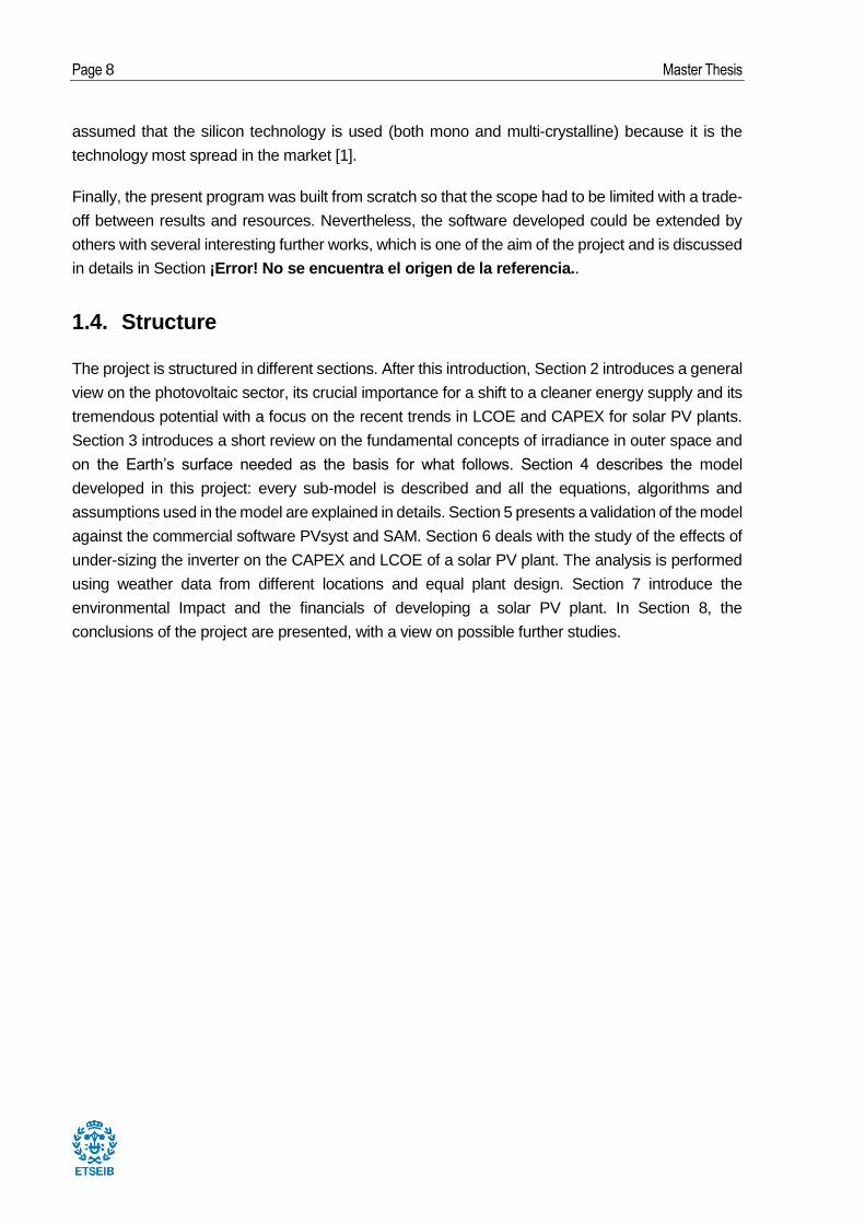
perspective, the PV market experienced a rocket growth in the last years: the global PV installed
capacity grew from 6.1GW in 2010 to 291GW in 2016, which means 47 times larger, which is clearly
visible in the figure below from [1]:
Figure 1: Commutative grid connected capacity in the years from 2006 to 2016 divided by macro-regions. Source IRENA [1]
The reasons for such a rapid growth of the PV market can be traced back to two main drivers.
Firstly, the policies for reduction of greenhouse gases emissions play a fundamental role and are
now present in the most of the countries, for example Europe set a target of 20% reduction of CO2
emissions by 2020 [3]. A clear example that shows the great impact of policies in the growth of
installed capacity is the situation the happened in Italy. There, thanks to subsidies and policy for a
profitable Feed-in Tariff, the PV market of the country grew rapidly during the years of the policy
that was available between 2005-2013. When the strong financial incentives were not available
anymore, annual installed capacity additions remained stable or even fell: added capacity in 2015
was 300MW while in 2014 it was 424MW. Nevertheless, the electricity generated by PV in the
country remains remarkably high, with 8.2% of the energy needs coming from PV in 2016 [2].
The second main reason is the reduction of LCOE of PV systems which makes it appealing for new
Page 10 Master Thesis
investors: this is actually both a driver and an effect because expansion driven by lower prices
brings economy of scales which further reduces the costs [4]. The LCOE is good indicator to
compare different technologies because it is independent of the specific technology as it represents
the all the costs of producing one unit of energy (Kwh, Mwh etc.) with a particular technology
considering the whole lifetime of the project. It can also be thought of as the minimum costs at
which energy should be sold to reach specific return on investment (for details on the formula of
LCOE and the models used in this work see section 4.12). For these reasons, the following section
is dedicated to a brief overview of the LCOE in PV systems.
2.1. LCOE of PV systems
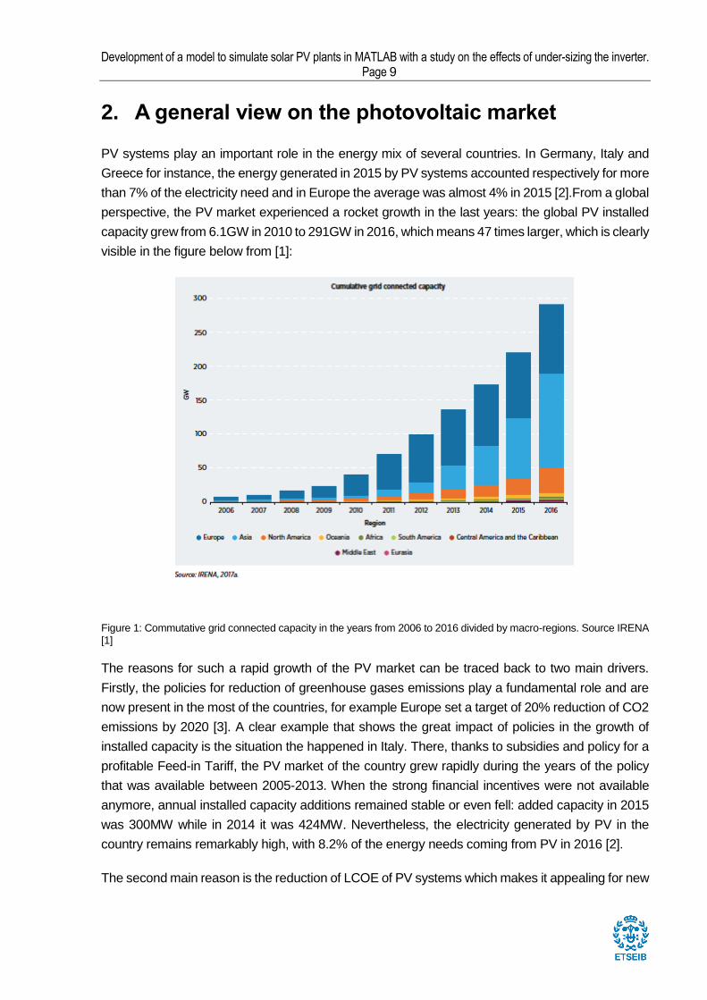
To have an idea of the trends of LCOE, the following graph compares the LCOE of the different
renewable energy sources (RES), with global averages from 2010 to 2017 elaborated by IRENA
[1]:
Figure 2 Levelized cost of electricity (LCOE) for different renewable energy technologies in 2010 and 2017 from global averages. Source IRENA [1].
The LCOE of solar photovoltaics has experienced a rapid drop of 72.2% in only 7 years, with values
around 0.36USD/KWh (or 360 USD/MWh) in 2010 compared to 0.1 USD/KWh (or 100 USD/MWh)
in 2017. In this case IRENA used weighted average cost of capital (WACC) of 7.5% for OECD
countries and china while 10% for the rest of the world (for a detailed description of WACC see
Section 4.12). It is interesting to see how the LCOE of PV projects is already in the fossil fuel LCOE
Development of a model to simulate solar PV plants in MATLAB with a study on the effects of under-sizing the inverter. Page 11
range, which means that the technology without subsidies is already cost competitive if compared
with conventional fossil fuel power generation. As a consequence, PV systems already reached
the grid parity in many countries [1].
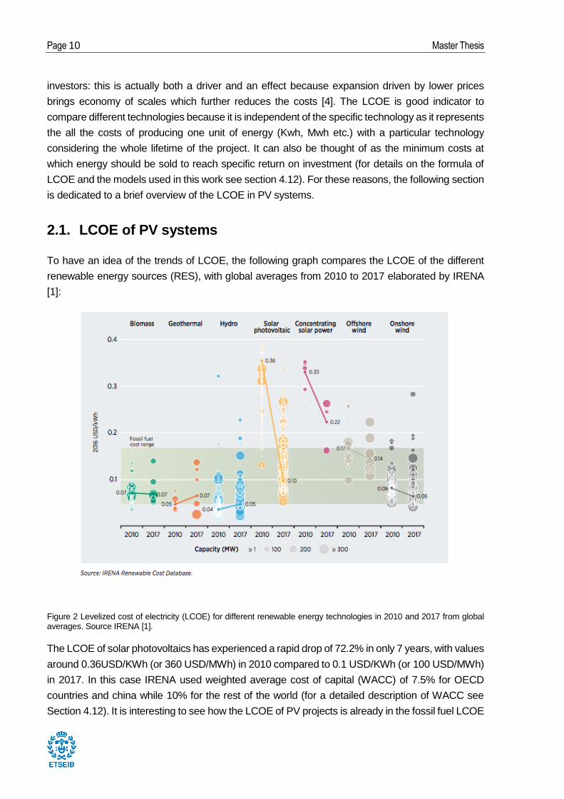
The main driver for this rapid drop in the LCOE is clearly the reduction in CAPEX that decreases
the investment needed to build a plant and the increase in capacity factor which increases the
amount of energy produced given the same plant. The figure below from IRENA [1] clearly shows
these trends:
Figure 3 Total installed cost, capacity factor and levelized cost of electricity (LCOE) for solar PV plants in the years from 2010 to 2017 (global averages). Source IRENA [1].
The installed cost fell from 4394 USD/kW in 2010 to 1388 USD/kW in 2017, while the capacity
factor grew from 0.14 to 0.18 in the same years, meaning that given the same amount of installed
power, a PV plant in 2017 generated on average 28.6% more than a plant in 2010. As a
consequence of these two factors, the LCOE on the right fell from 0.36USD/kWh to 0.10 USD/kWh
from 2010 to 2017.
The numbers above are global averages, with projects from all around the world, but clearly the
LCOE of a PV plant is very much related to its position and to the irradiance of the particular
location: with a higher average irradiance, the LCOE is expected to be lower. As an example, the
chart below shows the forecasted trend in LCOE (with real data from 2016) for a 1MW PV plant in
Madrid for different values of WACC [5]:
Page 12 Master Thesis
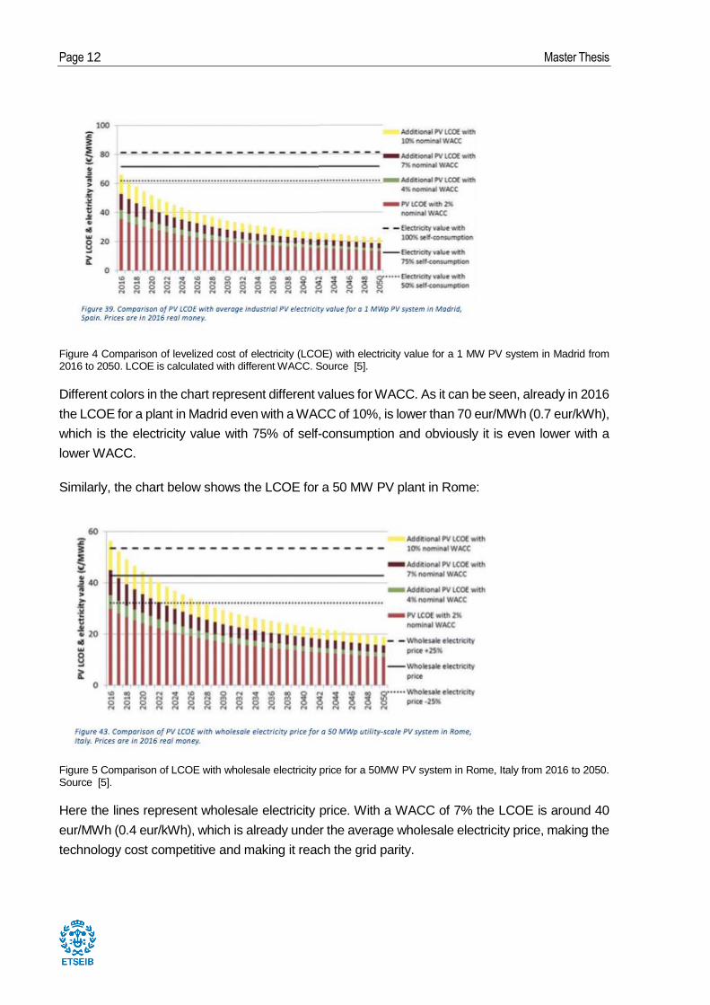
Figure 4 Comparison of levelized cost of electricity (LCOE) with electricity value for a 1 MW PV system in Madrid from 2016 to 2050. LCOE is calculated with different WACC. Source [5].
Different colors in the chart represent different values for WACC. As it can be seen, already in 2016
the LCOE for a plant in Madrid even with a WACC of 10%, is lower than 70 eur/MWh (0.7 eur/kWh),
which is the electricity value with 75% of self-consumption and obviously it is even lower with a
lower WACC.
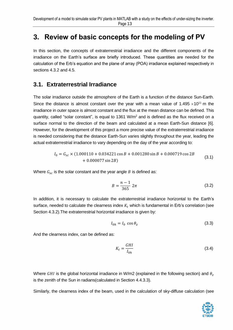
Similarly, the chart below shows the LCOE for a 50 MW PV plant in Rome:
Figure 5 Comparison of LCOE with wholesale electricity price for a 50MW PV system in Rome, Italy from 2016 to 2050. Source [5].
Here the lines represent wholesale electricity price. With a WACC of 7% the LCOE is around 40
eur/MWh (0.4 eur/kWh), which is already under the average wholesale electricity price, making the
technology cost competitive and making it reach the grid parity.
Development of a model to simulate solar PV plants in MATLAB with a study on the effects of under-sizing the inverter. Page 13
3. Review of basic concepts for the modeling of PV
In this section, the concepts of extraterrestrial irradiance and the different components of the
irradiance on the Earth’s surface are briefly introduced. These quantities are needed for the
calculation of the Erb’s equation and the plane of array (POA) irradiance explained respectively in
sections 4.3.2 and 4.5.
3.1. Extraterrestrial Irradiance
The solar irradiance outside the atmosphere of the Earth is a function of the distance Sun-Earth.
Since the distance is almost constant over the year with a mean value of 1.495 1011 m the
irradiance in outer space is almost constant and the flux at the mean distance can be defined. This
quantity, called “solar constant”, is equal to 1361 W/m2 and is defined as the flux received on a
surface normal to the direction of the beam and calculated at a mean Earth-Sun distance [6].
However, for the development of this project a more precise value of the extraterrestrial irradiance
is needed considering that the distance Earth-Sun varies slightly throughout the year, leading the
actual extraterrestrial irradiance to vary depending on the day of the year according to:
𝐼0 = 𝐺𝑠𝑐 × (1.000110 + 0.034221 cos𝐵 + 0.001280 sin𝐵 + 0.000719 cos 2𝐵
+ 0.000077 sin 2𝐵) (3.1)
Where 𝐺𝑠𝑐 is the solar constant and the year angle 𝐵 is defined as:
𝐵 =𝑛 − 1
365 2𝜋 (3.2)
In addition, it is necessary to calculate the extraterrestrial irradiance horizontal to the Earth’s
surface, needed to calculate the clearness index 𝐾𝑡 which is fundamental in Erb’s correlation (see
Section 4.3.2).The extraterrestrial horizontal irradiance is given by:
𝐼0ℎ = 𝐼0 cos 𝜃𝑧 (3.3)
And the clearness index, can be defined as:
𝐾𝑡 =𝐺𝐻𝐼
𝐼0ℎ (3.4)
Where 𝐺𝐻𝐼 is the global horizontal irradiance in W/m2 (explained in the following section) and 𝜃𝑧
is the zenith of the Sun in radians(calculated in Section 4.4.3.3).
Similarly, the clearness index of the beam, used in the calculation of sky-diffuse calculation (see

Page 14 Master Thesis
section 4.5.5) can be calculated as:
𝐾𝑏 =𝐵𝐻𝐼
𝐼0ℎ=𝐷𝑁𝐼
𝐼0 (3.5)
Where 𝐵𝐻𝐼 and 𝐷𝑁𝐼 are respectively the beam horizontal irradiance and the direct normal
irradiance explained in the following section.
3.2. The different components of the irradiance
In this section the concepts of global, diffuse, beam and direct normal irradiance are presented.
The extraterrestrial irradiance described in section 3.1 passes through the atmosphere before
reaching the Earth’s surface. During its journey, a part of it is absorbed, reflected, and diffracted by
the atmosphere. Therefore the irradiance reaching the surface of a module is lower and can be
seen as divided in two parts: a beam component, aligned with the direction of the sun beams, and
a diffuse component, coming from the reflection and diffraction of the atmosphere and the reflection
of the Earth’s surface (called albedo). Together they form the global irradiance. Since the irradiance
is a flux, it is important to define the orientation of the surface to which it is referred. Generally, the
irradiance is typically measured on a horizontal surface: global horizontal irradiance (GHI), diffuse
horizontal irradiance (DHI), and beam horizontal irradiance (BHI) are the three components
referred to a horizontal surface and are related by:
𝐺𝐻𝐼 = 𝐵𝐻𝐼 + 𝐷𝐻𝐼 (3.6)
Where 𝐵𝐻𝐼 is the projection of the direct normal irradiance (𝐷𝑁𝐼) on a horizontal surface:
𝐵𝐻𝐼 = 𝐷𝑁𝐼 cos 𝜃𝑧 (3.7)
𝐷𝑁𝐼 is the direct normal irradiance, which is the beam irradiance referred to a surface normal to
the direction of the sun. The zenith of the Sun is represented by 𝜃𝑧, which is the angle between
the direction of the sun and the vertical (see section 4.4.3.3 for more details). The relationship
above come from simple geometrical considerations:
Figure 6: Schematic showing the relationship between direct normal irradiance and beam horizontal irradiance
In the figure, Ib and Ibh represent respectively the beam irradiance (another name for DNI) and the

Development of a model to simulate solar PV plants in MATLAB with a study on the effects of under-sizing the inverter. Page 15
beam horizontal irradiance.
The values of GHI, DHI, BHI and DNI are needed for all the calculations of section 4.5.
In this project, it is always assumed that the global horizontal irradiance (and eventually the diffuse)
is always known a priori from measured data. As a consequence, no models to predict these values
starting from the extraterrestrial irradiance are treated in this work. It Is worth mentioning that
different models exist and more information on these models could be found in [6].
Page 16 Master Thesis
4. Model of the plant with MATLAB
4.1. Methodology
The model created in this project with MATLAB have the purpose of generating the hourly values
of several variables of a PV plant starting from hourly values of global horizontal irradiance and
temperature and, if available, diffuse horizontal irradiance and wind speed.
For the development of the present model the simulation software PVsyst developed by the
university of Genève is taken as the main reference for three reasons. First, because the software
is one of the most used in the industry as for example stated in [7]. Therefore, its simulation
approach is trusted. Second, because PVsyst has an in-depth approach into the models, providing
a high flexibility in the tuning of the parameters of every sub-model, which is precisely one of the
goals of the present project. Third, because the authors of PVsyst provide a thorough help manual
[8] which explains in details the reasoning behind the models with a pedagogical approach. The
software System Advisor Model (SAM) developed by NREL was used as a second reference when
the reasoning of PVsyst for some models (e.g. inverter model) could not be found or reproduced.
The same reasons listed above are valid for SAM which also provides a well explained manual [9].
The model is structured in different sub-models related to different physical quantities such as plane
of array (POA) irradiance current-voltage (I-V) characteristic, temperature of the cell etc. During the
development of the MATLAB model, the manuals of the software PVsyst and SAM were consulted
as guidelines [8], [9]. The books or articles cited by these manuals were carefully analyzed to obtain
the equations used in each particular model and implemented in MATLAB. Numerical algorithms
needed to solve the equations were implemented independently since the sources usually deal
only with analytical equations. For example, this was the case of the solver for systems of non-
linear equations used in the IV curve developed in section 4.6.2.
Each of the sub-models was validated comparing the hourly results of the software developed with
results of either PVsyst or SAM, depending on which software the sub-model was based on. In
addition, a validation of the whole model from measured irradiance to energy injected to the grid
was performed. Results of the validations can be found in section 5.
4.2. Model scope
The models for the following quantities are inside the scope of the project:
1. Diffuse horizontal to Global horizontal ratio (Erb’s correlation)
2. Position of the sun (Azimuth and Zenith)
3. Angle of incidence between sun and module
4. POA Incident beam irradiance
Development of a model to simulate solar PV plants in MATLAB with a study on the effects of under-sizing the inverter. Page 17
5. POA incident sky and ground diffuse irradiance
6. IAM factor for beam irradiance
7. Effective POA global irradiance
8. IV model reference parameters 𝐼𝐿,𝑟𝑒𝑓, 𝐼0,𝑟𝑒𝑓 and 𝑅𝑠,𝑟𝑒𝑓 calculated from 𝑅𝑠ℎ,𝑟𝑒𝑓 and 𝑎𝑟𝑒𝑓.
9. IV model parameters for any temperature and irradiance.
10. Temperature of the cell at any condition
11. Efficiency of the inverter at any voltage and power
12. Thermal losses in DC cables
13. AC cables and transformer losses
14. Automatic design of the layout: number of modules in series and parallel
15. LCOE of the project
All the above mentioned quantities are calculated hourly.
It is out of the scope of this project:
1. The synthetic generation of weather data from monthly averages.
2. The analysis of soling and spectral losses.
3. The analysis of mismatch losses due to problems in the MPPT.
4. The analysis of reactive and active power in the inverter.
4.3. Weather data and model of diffuse irradiance
4.3.1. Weather data
The weather data that the model can receive as inputs are: the global horizontal irradiance (GHI),
the diffuse horizontal irradiance (DHI), the ambient temperature and the wind speed. These
weather data are the main input of the model: ambient temperature and GHI are essential for the
execution of the software. Wind speed is optional, as explained in section 4.7. Ideally, also data for
DHI are needed, however they are not always available: in this case the Erb’s model is used to
estimate the diffuse irradiance from global irradiance through the clearness index as explained in
section 4.3.2. In the present project, it is assumed that at least ambient temperature and GHI are
always available as hourly measured values.
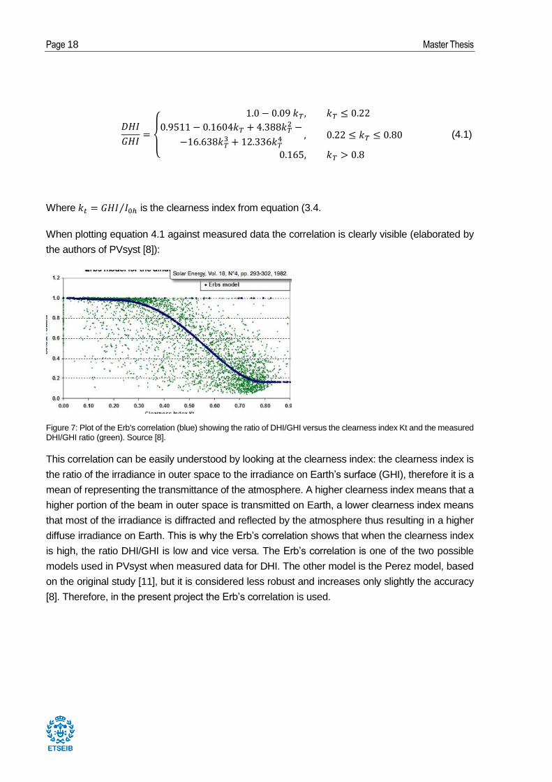
4.3.2. Model of the diffuse horizontal irradiance: The Erb’s correlation
The Erb’s correlation is used to find a ratio between diffuse horizontal irradiance and global
horizontal irradiance as a function of the clearness index. The relationship is taken from [6], based
on the original study [10], which is the same used by PVsyst [8], and is given by:
Page 18 Master Thesis
𝐷𝐻𝐼
𝐺𝐻𝐼=
1.0 − 0.09 𝑘𝑇 , 𝑘𝑇 ≤ 0.22
0.9511 − 0.1604𝑘𝑇 + 4.388𝑘𝑇2 −
−16.638𝑘𝑇3 + 12.336𝑘𝑇
4 , 0.22 ≤ 𝑘𝑇 ≤ 0.80
0.165, 𝑘𝑇 > 0.8
(4.1)
Where 𝑘𝑡 = 𝐺𝐻𝐼 𝐼0ℎ⁄ is the clearness index from equation (3.4.
When plotting equation 4.1 against measured data the correlation is clearly visible (elaborated by
the authors of PVsyst [8]):
Figure 7: Plot of the Erb's correlation (blue) showing the ratio of DHI/GHI versus the clearness index Kt and the measured DHI/GHI ratio (green). Source [8].
This correlation can be easily understood by looking at the clearness index: the clearness index is
the ratio of the irradiance in outer space to the irradiance on Earth’s surface (GHI), therefore it is a
mean of representing the transmittance of the atmosphere. A higher clearness index means that a
higher portion of the beam in outer space is transmitted on Earth, a lower clearness index means
that most of the irradiance is diffracted and reflected by the atmosphere thus resulting in a higher
diffuse irradiance on Earth. This is why the Erb’s correlation shows that when the clearness index
is high, the ratio DHI/GHI is low and vice versa. The Erb’s correlation is one of the two possible
models used in PVsyst when measured data for DHI. The other model is the Perez model, based
on the original study [11], but it is considered less robust and increases only slightly the accuracy
[8]. Therefore, in the present project the Erb’s correlation is used.

Development of a model to simulate solar PV plants in MATLAB with a study on the effects of under-sizing the inverter. Page 19
4.4. Model of the solar angles and angle of incidence
This section illustrates the procedure followed to calculate the angle of incidence (AOI) between
the direction of the sun beams and the normal to the plane of the module. The models needed to
calculate the AOI are: the model of the solar time, the equation of time and the solar angles. This
part of the software was based on the equations used by PVsyst [8].
4.4.1. Convention used in the weather data: the time shift
To understand what follows it is important to distinguish between solar and clock time. The solar
time is the time used for solar calculations and the solar noon is defined as the moment when the
Sun, in its apparent movement, passes exactly due south at the position of the observer. On the
other hand, the clock time is simply the time used in everyday life.
The weather data such as the GHI or the ambient temperature are usually given as hourly values
and are referred to a specific hour of the clock time. Each value is an average over an interval of
one hour and the present project uses the convention that the weather data are assumed to be
values at the middle of the hour interval. For example, the GHI corresponding to the hour interval
12-13 is considered to be the GHI reaching the modules at 12:30. This convention is used by most
weather centers and is followed by PVsyst [8]. The default convention can be modified by the user:
this step is fundamental in case the weather data used another convention because this time
difference affects heavily the calculations that follow. Moreover, the weather data refer to the clock
time, but the solar time is needed to calculate all the solar angles and the AOI. Therefore, the
conversion from clock to solar time is required. To sum up, the program calculates the AOI in three
steps: first, it sets the time shift to the default or user-defined convention; second, it converts the
clock time to the solar time; third, it calculates the solar angle and AOI based on the solar time.
4.4.2. Model of the solar time
In this section the procedure to convert the clock time to solar time is illustrated. The difference
between the solar and the clock time in hours can be expressed in a formula as follows:
𝑡𝑠 = 𝑡𝑐𝑙 − 𝑇𝑍 +𝜓𝑙𝑜𝑐15°
+ 𝐸𝑂𝑇 − 𝐷𝑆𝑇 (4.2)
Where 𝑇𝑍 is the time zone of the location in hours; 𝜓𝑙𝑜𝑐 is the longitude of the location in degrees
(East positive), 𝐸𝑂𝑇 is the equation of time in hours explained in the next section, and 𝐷𝑆𝑇 is the
daylight saving time in hours.
The difference between clock and solar time is caused by three main reasons:
1. The clock time refers to a time zone which refers to a specific meridian (for example UTC+1
means longitude=15*E). However, the specific longitude of the location is different from this
Page 20 Master Thesis
standard meridian therefore the solar time (which is referred to the observer local meridian)
will be different.
2. The Earth’s rate of rotation around the Sun varies during the year, leading to differences on
the time at which the Sun is due south. This is expressed by the EOT in section 4.4.2.1
3. The daylight-saving time (DST) might be present in the clock time depending on the region
and the season. This is a fictitious shift of time made by the society for energy saving
purposes, which clearly does not influence the real position of the Sun. Anyway, in the
software, the DST is set to zero by default as it is done in PVsyst (by default the weather
data are supposed to come without DST). It could be activated if the weather data are
recorded using the DST, or to show the output file with the clock time including DST.
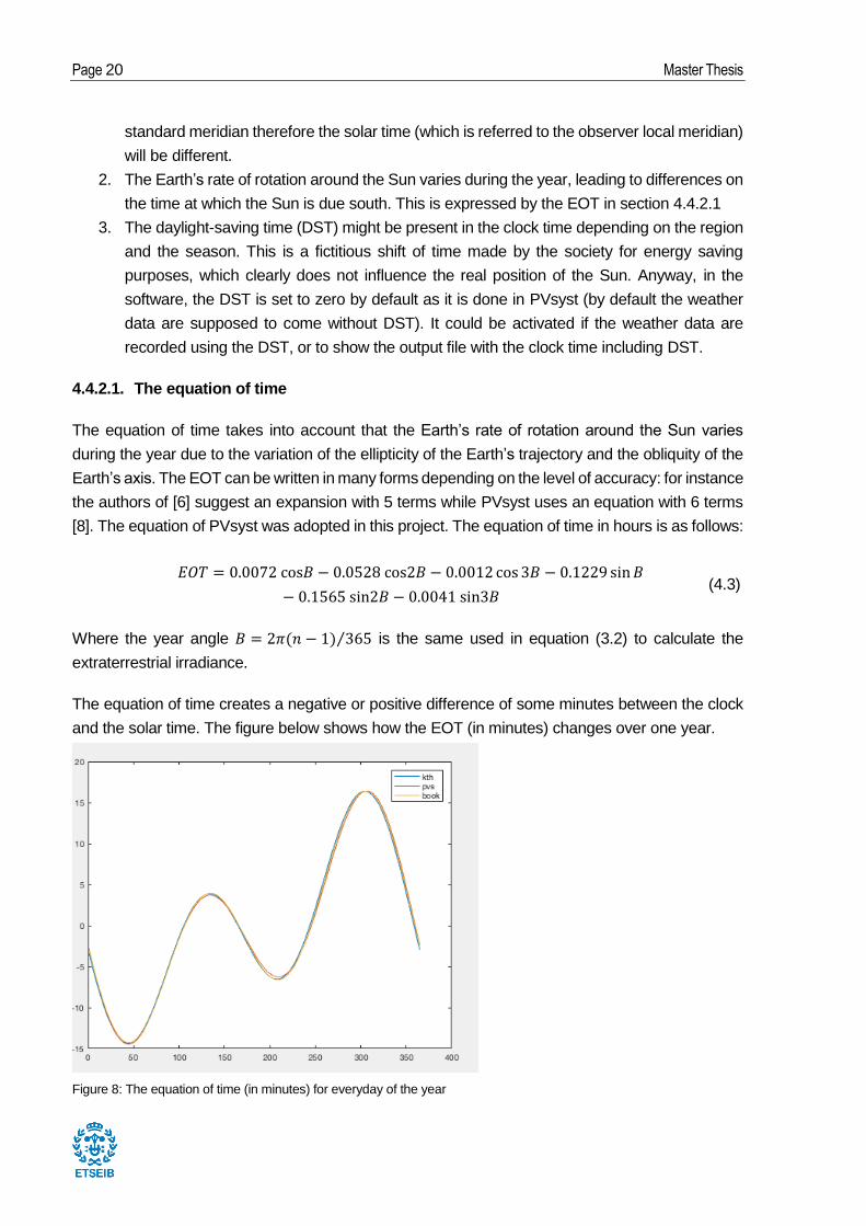
4.4.2.1. The equation of time
The equation of time takes into account that the Earth’s rate of rotation around the Sun varies
during the year due to the variation of the ellipticity of the Earth’s trajectory and the obliquity of the
Earth’s axis. The EOT can be written in many forms depending on the level of accuracy: for instance
the authors of [6] suggest an expansion with 5 terms while PVsyst uses an equation with 6 terms
[8]. The equation of PVsyst was adopted in this project. The equation of time in hours is as follows:
𝐸𝑂𝑇 = 0.0072 cos𝐵 − 0.0528 cos2𝐵 − 0.0012 cos3𝐵 − 0.1229 sin𝐵
− 0.1565 sin2𝐵 − 0.0041 sin3𝐵 (4.3)
Where the year angle 𝐵 = 2𝜋(𝑛 − 1) 365⁄ is the same used in equation (3.2) to calculate the
extraterrestrial irradiance.
The equation of time creates a negative or positive difference of some minutes between the clock
and the solar time. The figure below shows how the EOT (in minutes) changes over one year.
Figure 8: The equation of time (in minutes) for everyday of the year

Development of a model to simulate solar PV plants in MATLAB with a study on the effects of under-sizing the inverter. Page 21
As it can be seen, the maximum of the EOT is around day 300 (November), for which the solar
time is ahead of the clock time by 16 minutes, which is a relatively high number and thus it is
important to always consider the EOT when performing solar calculations.
4.4.3. Model of the solar angles
Once the solar time is computed, all the other solar angles are calculated according to the solar
time. In this section presents the procedure followed to obtain the solar angles: hour angle,
declination, solar azimuth and solar zenith (and altitude). In all the equations and in the software,
the angles are in radians.
4.4.3.1. Hour angle
The hour angle represents the position of the sun with respect to the specific location in angles. It
can be thought as the angular coordinate of the sun, if its position is projected on the plane of the
equator. The hour angle 𝜔, taken from PVsyst manual [8], is given by:
𝜔 =𝜋
12(𝑡𝑠 − 12) (4.4)
Where 𝑡𝑠 is the solar time from equation 4.2.
As it can be seen, the solar hour is zero when it is solar midday, which corresponds to the time at
which the Sun is exactly in its highest position in the sky dome at the specific location. The hour
angle gains 15 degrees every hour, because the Earth takes 24 hours to complete a rotation around
itself, which means it moves at a speed of 15 degrees/hour (360/24=15). This equation is derived
from geometrical considerations and is present in any book on the topic, for example [4], [6].
4.4.3.2. Declination
The declination can be seen as the angle between a line that connects the center of the sun with
the center of the Earth and the plane of the equator. The formula for the declination 𝛿, which is
taken from the PVsyst manual [8] is:
𝛿 =
asin (sin(𝐸𝐶𝐿) sin (2𝜋
𝑛 − 𝑛𝑜𝑟𝑖𝑔
𝑛𝑦𝑒𝑎𝑟)), 𝑛 ≤ 172
asin (sin(𝐸𝐶𝐿) sin(2𝜋𝑛 − 𝑛𝑜𝑟𝑖𝑔
𝑛𝑦𝑒𝑎𝑟) + 1.5 sin (2𝜋
𝑛 − 173
𝑛𝑦𝑒𝑎𝑟)), 𝑛 > 172
(4.5)
And:
𝑛𝑜𝑟𝑖𝑔 = 79 +MOD(𝑛, 4) 4⁄ (4.6)

Page 22 Master Thesis
Where: 𝐸𝐶𝐿 is the inclination between Earth’s axis and the ecliptic plane equal to 23.444° or
0.40917 radians, 𝑛 is the day of the year, 𝑛𝑜𝑟𝑖𝑔 is the year origin, 𝑛𝑦𝑒𝑎𝑟 are the days in one year
and MOD(𝑎, 𝑏) is the modulo function that represents the remainder of the division of a by b. This
last function is needed to take into account that non-leap year can actually be longer than 365 days
by quarters of a day, so that in 4 years another day is added obtaining a leap year of 366 days.
Again, other versions of these formulae are possible but it was preferred to follow the approach of
PVsyst [8] for consistency.
The declination changes with the day of the year from approx. -23.4 degrees to +23.4 degrees at
the winter and summer solstices respectively. The declination is also the main reasons why
seasons exist.
4.4.3.3. Sun zenith and azimuth
Sun zenith and azimuth are the two coordinates used to locate the position of the Sun in the sky
dome. The zenith is the angle between a vertical line and the direction of the Sun beam. The solar
altitude is the complementary angle of the Zenith. The azimuth is the angle between the south and
the projection of the Sun on the plane of the location. For a better understanding, the figure below
illustrates the two solar angles (together with the of the surface angles and the AOI discussed in
the following section):
Figure 9 Relevant angles of the position of the Sun, the orientation of the module and angle of incidence (AOI). Source [12].
Looking at the figure above, all the angles can be calculated with geometrical considerations. The
zenith 𝜃𝑧 is calculated as:
𝜃𝑧 = arccos(cosφcosδcosω + sinφsinδ) (4.7)

Development of a model to simulate solar PV plants in MATLAB with a study on the effects of under-sizing the inverter. Page 23
And the solar altitude 𝛼𝑠 is simply the complementary angle:
𝛼𝑠 =𝜋
2− 𝜃𝑧 (4.8)
The azimuth 𝛾𝑠 is given by:
𝛾𝑠 = sgn(ω) |arccos (cos𝜃𝑧sinφ − sin𝛿
sin𝜃𝑧cosφ)| (4.9)
Where φ is the latitude of the location in radians (positive in the northern hemisphere), δ and ω are
respectively hour angle and the declination discussed previously.
These equations are taken from the manual of PVsyst [8]. They are derived from geometrical
considerations and can be found in the same formulation in any book about solar photovoltaics,
such as [4], [6]. Note that the present program is written considering the solar zenith, while PVsyst
uses the solar altitude, so the cosines and sines are inverted since they are complementary angles.
This is just a matter of choice and the results are anyway equivalent.
4.4.4. Model of the angle of incidence between sun and panels
To calculate the angle of incidence (AOI) between the direction of the beams and the plane of the
module, two more angles (see Figure 9) defining the orientation of the module need to be specified:
1. The tilt angle 𝜃𝑡 of the module, which represent the angle between the plane of the module
and the ground
2. The azimuth γm of the module: angle between the orientation of the panel and due south.
With these two angles, and the two coordinates of the position of the Sun, the angle of incidence
can be finally calculated as:
𝜃𝐴𝑂𝐼 = arccos(𝑠𝑖𝑛𝜃𝑡sin𝜃𝑧 cos(γs − γm) + 𝑐𝑜𝑠𝜃𝑡cos𝜃𝑧) (4.1
0)
Again, the formula above is derived from geometrical considerations, and therefore can be found
in any book about this topic, such as [4], [6].
4.5. Model of the effective incident irradiance on the module
The incidence irradiance is the amount of solar energy that effectively reaches the cells of the
module. It is the main input of the model it affects almost linearly the power output of the modules.
The following graph shows how a generic IV curve changes under different irradiances:

Page 24 Master Thesis
Figure 10 Effects of the irradiance on the IV curve of a generic module. Source [13].
As shown above, the IV curve varies heavily with irradiance. The maximum power point varies
almost linearly with the irradiance and is clearly higher for higher irradiances (see Section 4.6.4),
while the voltage of the maximum power point increases only slightly.
4.5.1. Steps needed to calculate the incidence plane of array (POA) irradiance
The software calculates the hourly effective plane of array (POA) irradiance with the following steps:
1. The POA beam irradiance is calculated with the angle of incidence (AOI).
2. The POA ground-diffuse irradiance is calculated.
3. The POA sky-diffuse is calculated with Hay model.
4. The Incident Angle Modifier (IAM) is calculated on the beam component with the AOI.
5. The IAM factors for sky and ground diffuse is taken from a table given the array tilt.
6. The effective POA irradiance is found multiplying each component by its IAM loss.
Note that the approach followed here does not include an analysis of the self-shading due to
adjacent rows which is present in large scale solar PV plants but could not be implemented in this
project due to time and resources constrains. Nevertheless, it could be an interesting further study
as discussed in Section ¡Error! No se encuentra el origen de la referencia..
4.5.2. Model of the incidence plane of array (POA) irradiance
It is important to calculate the POA irradiance because the panels have a fixed tilt, therefore the
part of irradiance that is actually reaching the cells is going to be less than the total available
irradiance as it varies with the AOI varies: when the sun is low, e.g. at sunset and sunrise, the
available irradiance is lower. The POA irradiance can be thought of being composed by three parts:
beam, sky-diffuse and ground-diffuse:

Development of a model to simulate solar PV plants in MATLAB with a study on the effects of under-sizing the inverter. Page 25
𝐸𝑔 = 𝐸𝑏 + 𝐸𝑠𝑑 + 𝐸𝑔 (4.11)
Where Eb is the POA beam irradiance, Esd is the POA sky-diffuse irradiance and Eg is the POA
ground-diffuse irradiance.
The equation 4.10 represents only the irradiance reaching the surface of the module, without
considering the optical losses considered in the effective POA irradiance in Section 4.5.8.
4.5.3. Model of the POA beam irradiance
The POA beam irradiance is the part of the beam irradiance that reaches the plane of the array. It
is calculated by simply considering the projection of the DNI on the plane of the array by means of
the cosine of the angle of incidence. This is a geometrical transposition and therefore does not
imply any particular assumption. The same equation can be found in both SAM and PVsyst and all
the consulted sources [4], [6], [8], [9]. The beam irradiance 𝐸𝑏 effectively reaching the surface of
the panel is given by:
𝐸𝑏 = 𝐷𝑁𝐼 cos𝜃𝐴𝑂𝐼 (4.12)
Where 𝐷𝑁𝐼 is the direct normal irradiance in and 𝜃𝐴𝑂𝐼 is the angle of incidence AOI.
4.5.4. Model of the POA ground diffuse irradiance
The POA ground diffuse is the part of the ground diffuse irradiance that reaches the array. It is
calculated assuming that a part of irradiance reaching the Earth’s surface is reflected in an isotropic
way. Since it is reflected equally in any direction, the portion of this irradiance that reaches the
module can be calculated by mean of the view factor ( 1 − cos (𝜃𝑡) 2 ⁄ ) from the ground to the panel
[6]:
𝐸𝑔 = 𝐺𝐻𝐼 ∗ 𝜌1 − cos (𝜃𝑡)
2 (4.13)
Where 𝐺𝐻𝐼 is the global horizontal irradiance in W/m2, 𝜌 is the albedo of the ground and 𝜃𝑡 is the
tilt of the module.
The albedo is a factor that varies from 0 to 1 indicating the portion of irradiance that is reflected
from the ground, different kind of soils might have different values. The default value used in
PVsyst, and SAM is 0.2 [8], [9]. The same value will be used in the present project as a default
value.
The factor 1 − cos (𝜃𝑡) 2 ⁄ represents the view factor from the ground to a tilted surface. It is
Page 26 Master Thesis
calculated following the methodology explained in a study dedicated specifically on calculations of
the view factors needed in PV systems [14]. According to this study, the view factor between two
surfaces A1 and A2 is defined as:
𝐹12 =𝐷𝑖𝑓𝑓𝑢𝑠𝑒 𝑒𝑛𝑒𝑟𝑔𝑦 𝑓𝑟𝑜𝑚 𝐴1 𝑡ℎ𝑎𝑡 𝑟𝑒𝑎𝑐ℎ𝑒𝑠 𝐴2
𝑇𝑜𝑡𝑎𝑙 𝑑𝑖𝑓𝑓𝑢𝑠𝑒 𝑒𝑛𝑒𝑟𝑔𝑦 𝑓𝑟𝑜𝑚 𝐴1 (4.14)
This model is used in PVsyst and in SAM as the default and only model [8], [9]. Therefore, it was
used also in this project.
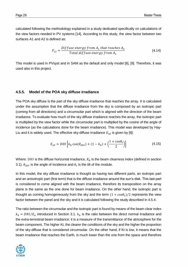
4.5.5. Model of the POA sky diffuse irradiance
The POA sky diffuse is the part of the sky diffuse irradiance that reaches the array. It is calculated
under the assumption that the diffuse irradiance from the sky is composed by an isotropic part
(coming from all directions) and a circumsolar part which is aligned with the direction of the beam
irradiance. To evaluate how much of the sky diffuse irradiance reaches the array, the isotropic part
is multiplied by the view factor while the circumsolar part is multiplied by the cosine of the angle of
incidence (as the calculations done for the beam irradiance). This model was developed by Hay-
Liu and it is widely used. The effective sky-diffuse irradiance 𝐸𝑠𝑑 is given by [8]:
𝐸𝑠𝑑 = 𝐷𝐻𝐼 [𝑘𝑏 cos(𝜃𝐴𝑂𝐼) + (1 − 𝑘𝑏) + (1 + cos𝜃𝑡
2)] (4.15)
Where: 𝐷𝐻𝐼 is the diffuse horizontal irradiance, 𝐾𝑏 is the beam clearness index (defined in section
3.1), 𝜃𝐴𝑂𝐼 is the angle of incidence and 𝜃𝑡 is the tilt of the module.
In this model, the sky diffuse irradiance is thought as having two different parts, an isotropic part
and an anisotropic part (first term) that is the diffuse irradiance around the sun’s disk. This last part
is considered to come aligned with the beam irradiance, therefore its transposition on the array
plane is the same as the one done for beam irradiance. On the other hand, the isotropic part is
thought as coming homogeneously from the sky and the term (1 + cos𝜃𝑡) 2⁄ represents the view
factor between the panel and the sky and it is calculated following the study described in 4.5.4.
The ratio between the circumsolar and the isotropic part is found by means of the beam clear index
𝑘𝑏 = 𝐷𝑁𝐼 𝐸𝑎⁄ introduced in Section 3.1. 𝑘𝑏 is the ratio between the direct normal irradiance and
the extra-terrestrial beam irradiance: it is a measure of the transmittance of the atmosphere for the
beam component. The higher Kt, the clearer the conditions of the sky and the higher the proportion
of the sky-diffuse that is considered circumsolar. On the other hand, if Kt is low, it means that the
beam irradiance that reaches the Earth, is much lower than the one from the space and therefore

Development of a model to simulate solar PV plants in MATLAB with a study on the effects of under-sizing the inverter. Page 27
the sky-diffuse is considered to be composed mainly of isotropic diffuse. More details are found in
Section 3.1
There are other models for the transposition of the sky-diffuse component on the plane of array,
such as the Perez model or the Hay, Davies, Klucher, Reindl (HDKR) sky diffuse model [6]. The
present project uses the Hay-Liu model presented above for the following reasons. It was the main
model used in PVsyst till 2015, because more complexes models such as the Perez model would
improve only slightly the accuracy while increasing the complexity. Moreover, the authors of PVsyst
state that the Perez model is less robust as much more sensible to the accuracy of the measured
data. Therefore, the Hay-Liu model is used in this project.
4.5.6. Model of the Incident Angle Modifier (IAM) for the beam component
The incident angle modifier (IAM) is an optical loss that considers that a part of the incoming beam
irradiance is reflected away by the module, and does not reach the cell. The IAM is defined as the
ratio between the transmittance at the specific AOI and the transmittance at AOI=0. The present
project uses the parametrization ASHRAE 93-3003:
𝐼𝐴𝑀 = 1 − 𝑏 (1
𝑐𝑜𝑠𝜃𝐴𝑂𝐼− 1) (4.16)
Where 𝑏 is a unitless fitting parameter and 𝜃𝐴𝑂𝐼 is the angle of incidence.
The equation is a parametrization to obtain a simple fit with just the parameter 𝑏. Physically, the
principle is described by Fresnel’s Law of reflection between two different media. The parameter 𝑏
is set to 0.05 as a default, following the default of PVsyst.
The higher the AOI, the higher the IAM losses as shown by the figure below:
Figure 11 Beam IAM losses for different angles of incidence (AOI) as calculated with ASHRAE 93-3003. Source [4]

Page 28 Master Thesis
This model was used as it is the default model because it is the default model used in PVsyst [8],
and because it is a standardized and simple model.
4.5.7. The incident angle modifier (IAM) for ground and sky diffuse
The IAM for the diffuse irradiance follows the same principles as IAM for the beam irradiance, with
the difference that the diffuse beams could come from any direction (here both ground and sky-
diffuse are considered to be isotropic). For this part, the same reasoning of PVsyst was followed,
but for sake of simplicity, since the IAM factors are considered to be constant given a tilt, the present
model does not compute the IAM in every simulation, instead it uses tabulated values that were
extrapolated from a batch simulation performed in PVsyst for different tilt angles.
To get this data, PVsyst performs the integral of the function for the IAM losses described in
equation (4.16) considering a beam that comes in all the possible directions from the sky according
to the isotropic model of sky-diffuse. The same reasoning applies to the ground-diffuse. The results
can be visualized in the following graphs which are taken from the detailed loss section of PVsyst
[15]:
Figure 12 Sky-diffuse and ground diffuse IAM losses versus plane tilt of the module. Source PVsyst software [15]
As it is shown, the IAM loss factor for ground-diffuse increases exponentially when the AOI
decreases while the IAM loss factor for sky-diffuse behaves almost symmetrically always between
4-5%. It should be noted that losses in ground-diffuse do not have a big impact in the overall system
because ground diffuse accounts for the smallest part of the effective irradiance.

Development of a model to simulate solar PV plants in MATLAB with a study on the effects of under-sizing the inverter. Page 29
4.5.8. Model of the effective plane of array irradiance (before shading)
The effective plane of array irradiance is the irradiance that actually reaches the surface of the PV
cells inside the module. It is the irradiance that will produce the photovoltaic effect, and will be the
input for the IV model. The effective POA irradiance is calculated without considering shading as
discussed in Section 4.5.1. The effective POA irradiance 𝐸𝑔 can be expressed as the sum of the
three components of the incident POA irradiance multiplied by its respective IAM factor as
calculated in the previous sections:
𝐸𝑔 = 𝑆𝐹(𝐸𝑏𝐼𝐴𝑀𝑏 + 𝐸𝑠𝑑𝐼𝐴𝑀𝑠𝑑 + 𝐸𝑔𝐼𝐴𝑀𝑔) (4.17)
Where 𝑆𝐹 is the soling factor, 𝐸𝑏 is the POA beam irradiance, 𝐸𝑠𝑑 is the POA sky-diffuse irradiance
and 𝐸𝑔 is the POA ground-diffuse irradiance. 𝐼𝐴𝑀𝑏, 𝐼𝐴𝑀𝑠𝑑 and 𝐼𝐴𝑀𝑔 are the IAM loss factors for
beam, sky-diffuse and ground-diffuse.
In the equation above, the only new parameter is the soling factor which considers losses due to
dirt on the panel. It is very challenging to accurately predict this factor, as it varies with wind speed,
precipitations, specific location, humidity etc. For this reasons in the present project this factor was
excluded from the analysis and it is set to 1 by default.
4.6. Model of the module I-V curve
A model of the current-voltage (I-V) curve of the PV module is fundamental as it determines how
much power can be generated by the module under any working condition. The power that can be
extracted from a PV module varies with irradiance (Figure 10), temperature (Figure 16) and the
working point of the I-V curve. Therefore, to perform the simulation and calculate the power
produced and the energy yield it is necessary to find a model that can create the I-V curve given
any external conditions of irradiance and temperature. When the I-V curve is known and the
working point is known, the power can be calculated at any moment by multiplying current and
voltage. The present project considers that the working point is always the maximum power point
(mismatch losses are out of the scope).
The following sections introduce the single diode model, the procedure used to solve the I-V curve
with this model and the assumptions on the model parameters needed to compute the I-V curve
when measured data are not available.
Page 30 Master Thesis
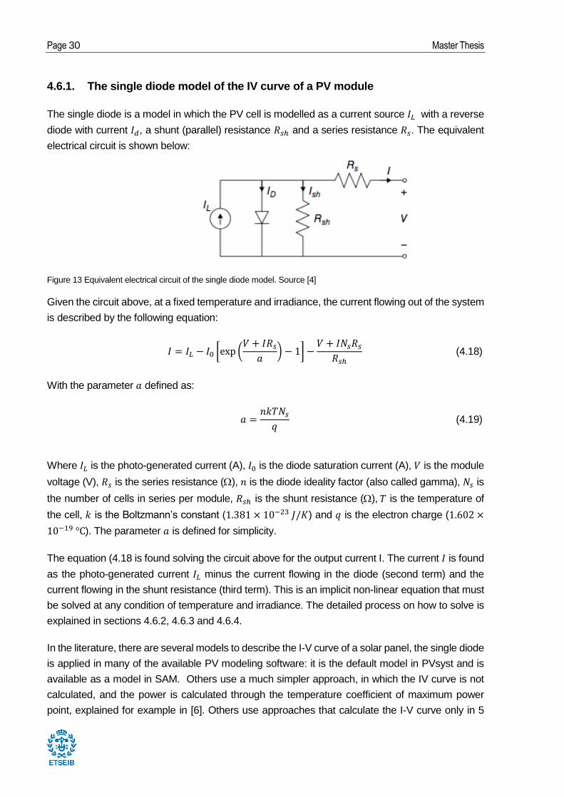
4.6.1. The single diode model of the IV curve of a PV module
The single diode is a model in which the PV cell is modelled as a current source 𝐼𝐿 with a reverse
diode with current 𝐼𝑑, a shunt (parallel) resistance 𝑅𝑠ℎ and a series resistance 𝑅𝑠. The equivalent
electrical circuit is shown below:
Figure 13 Equivalent electrical circuit of the single diode model. Source [4]
Given the circuit above, at a fixed temperature and irradiance, the current flowing out of the system
is described by the following equation:
𝐼 = 𝐼𝐿 − 𝐼0 [exp (𝑉 + 𝐼𝑅𝑠𝑎
) − 1] −𝑉 + 𝐼𝑁𝑠𝑅𝑠
𝑅𝑠ℎ (4.18)
With the parameter 𝑎 defined as:
𝑎 =𝑛𝑘𝑇𝑁𝑠𝑞
(4.19)
Where 𝐼𝐿 is the photo-generated current (A), 𝐼0 is the diode saturation current (A), 𝑉 is the module
voltage (V), 𝑅𝑠 is the series resistance (), 𝑛 is the diode ideality factor (also called gamma), 𝑁𝑠 is
the number of cells in series per module, 𝑅𝑠ℎ is the shunt resistance (), 𝑇 is the temperature of
the cell, 𝑘 is the Boltzmann’s constant (1.381 × 10⁻²³ 𝐽/𝐾) and 𝑞 is the electron charge (1.602 ×
10−19 °C). The parameter 𝑎 is defined for simplicity.
The equation (4.18 is found solving the circuit above for the output current I. The current 𝐼 is found
as the photo-generated current 𝐼𝐿 minus the current flowing in the diode (second term) and the
current flowing in the shunt resistance (third term). This is an implicit non-linear equation that must
be solved at any condition of temperature and irradiance. The detailed process on how to solve is
explained in sections 4.6.2, 4.6.3 and 4.6.4.
In the literature, there are several models to describe the I-V curve of a solar panel, the single diode
is applied in many of the available PV modeling software: it is the default model in PVsyst and is
available as a model in SAM. Others use a much simpler approach, in which the IV curve is not
calculated, and the power is calculated through the temperature coefficient of maximum power
point, explained for example in [6]. Others use approaches that calculate the I-V curve only in 5
Development of a model to simulate solar PV plants in MATLAB with a study on the effects of under-sizing the inverter. Page 31
points. More accurate models exist, like the 2 diodes models [16]. However, the approach followed
by PVsyst is to use the one diode model, and vary the value of the ideality factor to represent the
effect of two different diodes [8]. The authors claim that a more complex model is not needed as
the level of accuracy of the parameters from the manufacturers is not very high, and therefore a
high accuracy model would not lead to significant improvements. For these reasons, the single
diode model is implemented in this project.
4.6.2. Methodology to solve the IV curve
In the following sections, a method to solve the IV equation is presented, the method is based on
the procedure described in [6] with adjustments from the manual of PVsyst [8] and further
information based on studies describing the IV model used in PVsyst [7], [17], [18]. Equation (4.18
represents the relationship between current and voltage of a module at a fixed temperature and
irradiance. To solve for the current, 5 parameters are needed: 𝐼𝐿, 𝐼0, 𝑛, 𝑅𝑠 and 𝑅𝑠ℎ, which means
that in principle 5 equations are necessary to have a determined solution. The equation (4.18
describes the system at fixed temperature and irradiance with a set of 5 parameters, which means
that at any new condition of T and G, the 5 parameters must be recalculated.
The method presented here is composed of two steps: first, solving a system of equations to find
the unknown parameters at reference conditions (T=25C and G=1000) as presented in section
4.6.3 and then calculating the parameters at different temperature and irradiance as in explained
in 4.6.4.
4.6.3. Calculation of the IV parameters at reference conditions
In this section, the parameters of the equation (4.18 at reference condition are calculated (from now
on referred to as reference parameters). In everything that comes next, the irradiance and the
temperature of the cell is supposed to be known at standard conditions. In addition, from the PV
module datasheet, the following parameters are considered to be known at standard conditions:
𝑉𝑂𝐶, 𝐼𝑆𝐶, 𝐼𝑚𝑝𝑝, 𝑉𝑚𝑝𝑝 and 𝜇𝐼𝑠𝑐, respectively voltage at open circuit condition, short circuit current,
voltage at maximum power point, current at maximum power point, and temperature coefficient of
the short circuit current. These parameters are always available in PV datasheets.
The equation of the IV curve present 5 unknown parameters, so in principle 5 equations are
needed. The procedure described in [6] suggests to create the system by finding 5 conditions from
the PV datasheet. The first three conditions are the known points of the IV curve: short circuit
current, open circuit voltage and voltage and current at maximum power point. The fourth condition
is setting the derivative of I-V curve equal to zero in its maximum in the known maximum power
point. The fifth condition is setting the derivative of the open circuit voltage equal to the temperature
coefficient of the open circuit voltage. These five conditions result in the following set of equations:

Page 32 Master Thesis
𝐼𝑠𝑐,𝑟𝑒𝑓 = 𝐼𝐿,𝑟𝑒𝑓 − 𝐼0,𝑟𝑒𝑓 [exp(𝐼𝑠𝑐,𝑟𝑒𝑓𝑅𝑠,𝑟𝑒𝑓
𝑎𝑟𝑒𝑓) − 1] −
𝐼𝑠𝑐,𝑟𝑒𝑓𝑅𝑠,𝑟𝑒𝑓
𝑅𝑠ℎ,𝑟𝑒𝑓 (4.20)
𝐼𝐿,𝑟𝑒𝑓 = 𝐼0,𝑟𝑒𝑓 [exp (𝑉𝑜𝑐,𝑟𝑒𝑓
𝑎𝑟𝑒𝑓) − 1] +
𝑉𝑜𝑐,𝑟𝑒𝑓
𝑅𝑠ℎ,𝑟𝑒𝑓 (4.21)
𝐼𝑚𝑝,𝑟𝑒𝑓 = 𝐼𝐿,𝑟𝑒𝑓 − 𝐼0,𝑟𝑒𝑓 [exp(𝑉𝑚𝑝,𝑟𝑒𝑓+𝐼𝑚𝑝,𝑟𝑒𝑓𝑅𝑠,𝑟𝑒𝑓
𝑎𝑟𝑒𝑓) − 1] −
𝑉𝑚𝑝,𝑟𝑒𝑓+𝐼𝑠𝑐,𝑟𝑒𝑓𝑅𝑠,𝑟𝑒𝑓
𝑅𝑠ℎ,𝑟𝑒𝑓 (4.22)
𝐼𝑚𝑝,𝑟𝑒𝑓
𝑉𝑚𝑝,𝑟𝑒𝑓=
𝐼0,𝑟𝑒𝑓𝑎𝑟𝑒𝑓
exp (𝑉𝑚𝑝,𝑟𝑒𝑓+𝐼𝑚𝑝,𝑟𝑒𝑓𝑅𝑠,𝑟𝑒𝑓
𝑎𝑟𝑒𝑓) +
1𝑅𝑠ℎ,𝑟𝑒𝑓
1 +𝐼0,𝑟𝑒𝑓𝑅𝑠,𝑟𝑒𝑓𝑎𝑟𝑒𝑓
exp (𝑉𝑚𝑝,𝑟𝑒𝑓+𝐼𝑚𝑝,𝑟𝑒𝑓𝑅𝑠,𝑟𝑒𝑓
𝑎𝑟𝑒𝑓) +
𝑅𝑠,𝑟𝑒𝑓𝑅𝑠ℎ,𝑟𝑒𝑓
(4.23)
𝜕𝑉𝑜𝑐𝜕𝑇
= 𝜇𝑣,𝑜𝑐 ≅𝑉𝑜𝑐(𝑇𝑐) − 𝑉𝑜𝑐(𝑇𝑐,𝑟𝑒𝑓)
𝑇𝑐 − 𝑇𝑐,𝑟𝑒𝑓 (4.24)
Where the variables with the subscript ‘ref’ are at reference conditions of T=25C and
G=1000W/m2: 𝐼𝑠𝑐,𝑟𝑒𝑓 is the short circuit current (A), 𝐼𝐿,𝑟𝑒𝑓 is the photo-generated current (A), 𝐼0,𝑟𝑒𝑓
is the diode saturation current (A), 𝑅𝑠,𝑟𝑒𝑓 is the series resistance (), 𝑎𝑟𝑒𝑓 is the parameter defined
above in equation (4.19), 𝑅𝑠ℎ,𝑟𝑒𝑓 is the shunt resistance (), 𝑉𝑜𝑐,𝑟𝑒𝑓 is the open circuit voltage (V),
𝐼𝑚𝑝,𝑟𝑒𝑓 is the current at maximum power point (A), 𝑉𝑚𝑝,𝑟𝑒𝑓 is the voltage at maximum power point
(V), 𝜇𝑉𝑜𝑐 is the temperature coefficient of the open-circuit voltage (V/C) and 𝑇𝑐,𝑟𝑒𝑓 is the
temperature of the cell (C).
In theory, solving simultaneously this set of equations should provide the five parameters at
reference conditions. However, in the manual of PVsyst, the authors, referring to this approach,
suggest to avoid using all the five equations to solve the system because it would often lead to
solution with no physical meaning as the parameters could be out of their physical range, (e.g. the
ideality factor greater than 2 etc). The authors of PVsyst suggest instead to limit the number of
unknowns by setting 𝑅𝑠ℎ,𝑟𝑒𝑓 to a default value (which might be changed or measured as explained
in 4.6.4 and 4.6.6), and guessing 𝑅𝑠,𝑟𝑒𝑓, thus remaining with only 3 unknowns: 𝐼𝐿,𝑟𝑒𝑓, 𝐼0,𝑟𝑒𝑓 and
𝑛 and using only the first three equations above to solve the system [8], [18]. Once the system is
solved, PVsyst proposes different ways to find the actual 𝑅𝑠,𝑟𝑒𝑓 as explained in section 4.6.4. This
project follows the same method as PVsyst as it is proven that achieve great accuracy [6] thus
leading to a system composed by only the three equations from (4.20) to (4.22).
To solve this system of three nonlinear equations, different numeric methods could be used such
as Newton method for systems, but for the sake of simplicity, the inbuilt MATLAB function fsolve
will be used, also because which proved to be rapid and effective when running the program.

Development of a model to simulate solar PV plants in MATLAB with a study on the effects of under-sizing the inverter. Page 33
To reduce the computational time when solving such a complex nonlinear system, an accurate
initial guess for the variables is needed. The authors of [6] provide a guideline on how to guess the
parameters:
1. 𝐼𝐿,𝑟𝑒𝑓,𝑔𝑢𝑒𝑠𝑠 is guessed to be equal to Isc because at short circuit condition the other two
terms of the equation are very small:
𝐼𝐿,𝑟𝑒𝑓,𝑔𝑢𝑒𝑠𝑠 = 𝐼𝑠𝑐,𝑟𝑒𝑓 (4.25)
2. 𝐼0,𝑟𝑒𝑓,𝑔𝑢𝑒𝑠𝑠 is guessed by neglecting the last term and the -1 from the equation at open
voltage (eq. (4.21):
𝐼0,𝑟𝑒𝑓,𝑔𝑢𝑒𝑠𝑠 = 𝐼𝑠𝑐,𝑟𝑒𝑓 exp(−𝑉𝑜𝑐,𝑟𝑒𝑓
𝑎𝑟𝑒𝑓,𝑔𝑢𝑒𝑠𝑠) (4.26)
3. 𝑅𝑠,𝑟𝑒𝑓,𝑔𝑢𝑒𝑠𝑠 is guessed by inserting all the guess values in the equation at maximum power
point (eq. (4.22) neglecting the last term and the -1:
𝑅𝑠,𝑟𝑒𝑓,𝑔𝑢𝑒𝑠𝑠 =
𝑎𝑟𝑒𝑓,𝑔𝑢𝑒𝑠𝑠 (log (𝐼𝐿,𝑟𝑒𝑓,𝑔𝑢𝑒𝑠𝑠 − 𝐼𝑚𝑝,𝑟𝑒𝑓
𝐼0,𝑟𝑒𝑓,𝑔𝑢𝑒𝑠𝑠) − 𝑉𝑚𝑝,𝑟𝑒𝑓)
𝐼𝑚𝑝,𝑟𝑒𝑓
(4.27)
With the above guesses the system can always be solved smoothly and with a limited amount of
computational power. Note that the unknown parameters need to be found only once per panel,
and then they are saved in the software. Instead, for the parameters at any T and G, that need to
be calculated hourly, there is no need to solve the nonlinear system again. In facts, the parameters
just need to be recalculated according to the specific T and G, which does not imply solving a
system, but only simple equations and the implicit I-V equation as explained in section 4.6.4.
Therefore, the resulting computational load and time is not particularly heavy and a whole
simulation, that calculates I-V curves and working points every hour, can be performed in less than
25 seconds (depending on the CPU of the computer).
4.6.4. Calculation of the IV parameters at any given temperature and irradiance
In this section, the method to find the 5 unknown parameters: Rs, Rsh, Gamma, Iph, Io of the single
diode model at any temperature and irradiance is illustrated. It is assumed that the value of Rs is

Page 34 Master Thesis
independent of temperature and irradiance, as assumed by [6] and PVsyst [9]. The other
parameters are calculated with equations that relate the reference value of the parameter with the
new value of the parameter as a function of irradiance or temperature (or both).
4.6.4.1. The photo-generated current
The photo-generated current is a function of the irradiance and the temperature given by:
𝐼𝐿(𝐺, 𝑇) =𝐺
𝐺𝑟𝑒𝑓[𝐼𝐿,𝑟𝑒𝑓 + 𝜇𝐼𝑠𝑐(𝑇 − 𝑇𝑟𝑒𝑓)] (4.28)
Where: 𝐺 is the irradiance in W/m2, 𝐺𝑟𝑒𝑓 is the irradiance at standard conditions (1000 W/m2), 𝜇𝐼𝑠𝑐
is the temperature coefficient of the short circuit current (C/A).
The photo-generated current is proportional to the incoming irradiance, and increases slightly with
temperature (the value of the temperature coefficient on short circuit current is of the order of
0.05%/C).
4.6.4.2. The diode reverse saturation current
The diode reverse saturation current varies only with temperature according to:
𝐼0(𝑇) = 𝐼0,𝑟𝑒𝑓 (𝑇
𝑇𝑟𝑒𝑓)
3
exp [𝑞휀𝐺𝑛𝑘
(1
𝑇𝑟𝑒𝑓−1
𝑇)] (4.29)
Where 휀𝐺 is the bandgap equal to 1.12eV for crystalline silicon.
The above two equations are taken from [6] and are the same used in PVsyst [8]. Note that in [6]
the authors propose an equation to vary 휀𝐺 according to the temperature, instead in PVsyst 휀𝐺 is
considered to be constant [8]. The approach of PVsyst was followed, also because the variation of
휀𝐺 is anyway very small and its impact on the IV curve is negligible.
4.6.4.3. The shunt resistance
For the shunt resistance, the authors of PVsyst propose an empirical model introduced with an
experimental study [18] and further discussed by other authors [7]. Following this approach, the
shunt resistance is modeled as having an exponential behavior:
𝑅𝑠ℎ(𝐺) = 𝑅𝑠ℎ,𝑏𝑎𝑠𝑒 + (𝑅𝑠ℎ,0 − 𝑅𝑠ℎ,𝑏𝑎𝑠𝑒) exp (−𝑅𝑠ℎ,𝐸𝑥𝑝 (𝐺
𝐺𝑟𝑒𝑓)) (4.30)
And:

Development of a model to simulate solar PV plants in MATLAB with a study on the effects of under-sizing the inverter. Page 35
𝑅𝑠ℎ,𝑏𝑎𝑠𝑒 = 𝑚𝑎𝑥 [(𝑅𝑠ℎ,𝑟𝑒𝑓 − 𝑅𝑠ℎ,0 exp(−𝑅𝑠ℎ,𝑒𝑥𝑝)
1 − exp(−𝑅𝑠ℎ,𝑒𝑥𝑝)) , 0] (4.31)
Where: 𝑅𝑠ℎ,0 and 𝑅𝑠ℎ,𝑏𝑎𝑠𝑒 are empirical parameters in .
The above equation models the shunt resistance 𝑅𝑠ℎ as having an exponential increase at low
irradiances. Recalling that a higher 𝑅𝑠ℎmeans less losses, this adjustment increases the efficiency
at low irradiances, and overall increases the accuracy of the IV model [18]. The exponential
behavior of 𝑅𝑠ℎ when varying the irradiance, is illustrated below from [18]:
Figure 14 Shunt resistance as a function of the irradiance. Source [18].
4.6.4.4. The ideality factor gamma
For the ideality factor gamma, the default approach of PVsyst was to consider it constant and
independent of temperature and irradiance [8]. Later, they introduced an empirical parameter 𝜇𝛾 to
vary gamma with temperature so that the derivative of the maximum power point with respect to
the temperature can be adjusted with the temperature coefficient of Pmp provided by the
manufacturer datasheet as explained in PVsyst manual [8] and further discussed in [17]. In the
present project, the value of 𝜇𝑛 is not calculated but can be inserted externally to be a model
parameter of the module. The reasoning performed by PVsyst is anyway explained for a better
understanding. According to this approach, gamma varies with temperature according to:
𝑛(𝑇) = 𝑛𝑟𝑒𝑓 + 𝜇𝑛(𝑇 − 𝑇𝑟𝑒𝑓) (4.32)
Page 36 Master Thesis
The adjustment can be understood visually by looking at:
Figure 15 Maximum power as a function of the temperature for three different models and comparison with measurement data. Source [17]
Where 𝜇𝑃𝑚𝑝𝑝,𝑁𝑃is the value of the datasheet and 𝜇𝑃𝑚𝑝𝑝,𝑆𝑙𝑜𝑝𝑒is the value of the model.
The authors of PVsyst warn that the value of the 𝜇𝑃𝑚𝑝𝑝 provided in the datasheet of the modules
might not be representative of the behavior of the module in real conditions, because the
manufacturers provide just one value of 𝜇𝑃𝑚𝑝𝑝 usually measured at 25 C, while instead it itself
changes with temperature. Therefore, in PVsyst the correction of gamma to obtain the same 𝜇𝑃𝑚𝑝𝑝
as the one in the datasheet is an option of the user. The same approach was followed in the
developing of this software, if the value of 𝜇𝑃𝑚𝑝𝑝 can be found in an external database, which is
usually possible for example from SAM and PVsyst that provide an update database of modules.
4.6.5. Calculation of the IV curve and maximum power point given all the
parameters
In this section, the method to calculate the points of the IV curve and the maximum power point is
presented. Once all the parameters of the IV curve are calculated at the specific temperature and
irradiance (as explained in section 4.6.4), IV equation is finally fully described. Still, the single diode
equation (4.18) is an implicit equation, because the current appears in both sides of the equation,
therefore it cannot be solved analytically. In the present project this equation is solved numerically
through a simple Newton Method taken from [19], that was chosen because it has proven to
converge to a solution in few cycle and with limited computational time.
To find the I-V curve and the maximum power point, the algorithm used proceeds in the following

Development of a model to simulate solar PV plants in MATLAB with a study on the effects of under-sizing the inverter. Page 37
way. First, an equally spaced vector of voltage from 0 to Voc is generated, then the newton method
finds for each voltage the corresponding current by iterating till the difference between two steps is
smaller than a given tolerance. Second, only the positive values of the current are kept with their
respective voltage: the two vectors of voltage and current fully describe IV curve. Third, to find the
power, the values of the vectors of voltage and current are multiplied. Finally, the maximum power
point is the calculated as the numerical maximum of the power vector. Moreover, the program
saves also Imp and Vmp, respectively current and voltage corresponding to the maximum power
point needed for the calculation of the inverter losses and the losses in the DC cables discussed in
sections 4.9 and 4.10.1 respectively.
In this project, the array is supposed to work always at maximum power point thanks to the MPPT.
Therefore the Pmp, Imp and Vmp found above are considered to be the output of a module of a
string. Sequentially, they are then multiplied by respectively the number of modules in an array, the
number of modules in parallel, and the numbers of module in strings to obtain the power, current
and voltage of the array as discussed in section 4.8.1. These values will be the input of the inverter
model 4.9.
Note that in this procedure, the maximum power, current and voltage were calculated through the
maximum of a numeric array. One could claim that this reduces the accuracy to the number of
equally spaced points previously defined for the voltage vector chosen at the beginning. And for
example, in [6] the authors present an analytical way to find the maximum working point. However,
calculating the maximum power point analytically would add unnecessary computational power
because the software already produces results with a root mean square error compared to the DC
power of PVsyst lower than 0.27% as explained in section 5. Lastly, for this procedure, an explicit
algorithm from PVsyst has not been found, therefore the algorithm explained above was chosen
due to its high accuracy and low computational power.
4.6.6. Assumptions on the parameters of the IV curve and methods to find them
experimentally.
This section is divided in two parts, the first one introduces the assumptions made to set default
parameters for the I-V model when only the data from datasheet are available and the second part
briefly shows possible methods to find these parameters experientially.
As explained in section 4.6.3, to calculate the single diode model and the I-V equation at standard
conditions, 5 parameters are needed: Rsh, Rs, n, Iph, Io. However, since Rs, Ioh and Iph and Io
are calculated with the resolution of the system, only two parameters are needed: gamma and Rsh.
In addition, to calculate how these parameters vary with temperature and irradiance as shown in
section 4.6.4, other two parameters are needed: Rshexp and Rsh0. Therefore, a total of four
parameters: gamma, Rsh, Rshexp, Rsh0, must be either assumed or measured for the model to
work properly.

Page 38 Master Thesis
If the only available data are the one from the manufacturer datasheet, the parameters will be
assumed following the same assumptions used in PVsyst, given their extensive experience in the
field and continuous updating to new technologies.
For the value of gamma, the default value will be n=1.05 for mono-crystalline and 1.1 for
polycrystalline as considered in PVsyst [8].
For the Rsh, if an IV curve is available, it could be calculated as the inverse of the slope of the I-V
curve at short circuit, but it is not implemented in the model (the operation should be performed
graphically). Otherwise, the method to find the default value proposed by PVsyst equal to 400Ω will
be used for crystalline silicon.
The value of Rshexp is set equal to 5.5 as the authors of PVsyst say it produces good results for
almost all the modules they have tested [8], [18].
The value of Rsh_0 is set as Rsh0 =4* Rshref as suggested by the authors of PVsyst, even though
they add a notice to explain that computing this ratio with great accuracy is problematic because of
complications in the measurements of the slope of the IV curve at low irradiances [8].
The assumptions considered above are needed if the only available data is from the module
datasheets. On the other hand, if experimental tests could be performed on the module to measure
its IV curve at different conditions, there are different methods to calculate the parameters so that
the produced IV curve has the closest fit to the measured data. This alone is an extensive topic
and it is out of the scope of the present project. Nevertheless, during the development of the present
project, two possible methods to perform this optimization were found and are mentioned here for
the interest of the reader. The first one proposes a method based on a numerical optimization which
finds the set of reference parameters that best fits their measured data at different irradiance [7].
The second one builds up on the first one and continues a similar study not only limited at varying
the irradiance but also varying the temperature and compares different modeling approaches [17].
Clearly, the computational power increases with the complexity of the optimization algorithm, but
this might be justified in an advanced phase of modeling of a project in which few possible PV panel
models were selected and an accurate simulation is needed to assess the different characteristics
with high accuracy. However, in the present model the assumptions made above already constitute
an accurate model and anyway all the parameters can be changed by the user. Therefore, if more
accurate assumptions of the parameters were available, they could be inserted in the model.
4.6.7. Summary of the steps needed to calculate the hourly power generated with
the single diode model of the IV curve
In this section, a summary of the necessary steps to obtain the hourly maximum power point
generated by the PV panel through the single diode model is presented. The steps are as follows:

Development of a model to simulate solar PV plants in MATLAB with a study on the effects of under-sizing the inverter. Page 39
Steps that are computed once for PV module model:
1. A PV module is chosen with at least the following information: Impp, Vmpp, Isc, Voc muIsc
at T=25C and G=1000W/m2, Ns, and the cell area Ac.
2. In case the parameters to model the IV curve are available from a database, skip to step 7.
3. Rsh and gamma are guessed as explained in 4.6.6.
4. The system of 3 nonlinear equations is solved to obtain the 3 missing parameters I_L, Io
and Rs at reference conditions according to 4.6.3.
5. The set of reference parameters is saved in a struct and it is linked to the struct of the
module.
Steps that are computed every hour:
6. The 5 parameters are calculated with the specific temperature and irradiance, as explained
in 4.6.4.
7. The IV curve is calculated in each point, current and voltage are saved in vectors. The
power is found as element-by-element multiplication of the two according to 4.6.5.
8. The output DC power, voltage and current of the module are calculated as the numerical
maximum of the power Pmp and its corresponding voltage Vmp and current Imp as
explained in 4.6.5.

Page 40 Master Thesis
4.7. Model of the temperature of the PV module
In this section, the procedure followed to calculate the hourly temperature of the cells of the module
is explained.
4.7.1. The effects of temperature on the I-V curve
It is important to know the temperature of the cell because it affects the whole I-V curve. When the
temperature increases, the open circuit voltage decreases, the short circuit current increases
slightly and the maximum power point decreases. As a consequence, at a given irradiance, if the
temperature increases, the electrical efficiency of the module decreases leading to a lower power
extraction. These effects are explained visually by the figure below that represents a generic
module at fixed irradiance and different temperatures:
Figure 16 Effects of the temperature on the IV curve of a generic PV module. Source [13].
4.7.2. The temperature from an energy balance
To estimate the cell temperature, there are different approaches in the literature, the approach
followed in this project is the one described in [4] which comes from an experimental study [20].
This approach was chosen for two main reasons. Firstly because with few parameters it provides
sufficient accuracy: the temperature difference against measurements is within a range of 2C,
resulting in an error in the range of 1% in DC power against measured data by the authors [20].
Secondly because it is the one used in PVsyst [8].
The approach is based on an energy balance across the PV module, that receives heat from the
irradiance of the sun and it is cooled by conduction with ambient air and by convection with the

Development of a model to simulate solar PV plants in MATLAB with a study on the effects of under-sizing the inverter. Page 41
wind. Following this reasoning, the temperature of the cell can be written as follows:
𝑇𝑐 = 𝑇𝑎 +𝛼𝐸𝑒(1 − 𝜂𝑚)
𝑈0 + 𝑈1𝑣𝑤 (4.33)
And the efficiency of the module is given by:
𝜂𝑚 =𝑃𝑑𝑐𝐸𝑒𝐴𝑐
(4.34)
Where: 𝑇𝑐 is the temperature of the module (C), 𝑇𝑎 is the temperature of the surroundings (C), 𝛼
is the adsorption coefficient, 𝐸𝑒 is the POA effective global irradiance on the module (W/m2), 𝜂𝑚 is
the electrical efficiency of the module, 𝑈0 is the constant heat transfer coefficient (W/ C m2), 𝑈1 is
the convective heat transfer coefficient (W/C m2/m/s), 𝑣𝑤 is the wind speed (m/s), 𝑃𝑑𝑐 is the
electrical power (W) and 𝐴𝑐 is the area occupied by the cells (m2).
The nominator of equation (4.33) represents the part of the incoming solar energy that contributes
to heat up the module. This differs from the total incoming POA irradiance because part of the
incoming irradiance is transformed into electricity by the photovoltaic effect (considered with the
electrical efficiency 𝜂𝑚) and another part is reflected by the module (considered through the
adsorption coefficient 𝛼). The denominator represents the overall heat transfer coefficient that the
incoming power to a change in temperature.
To solve equation (4.33 for the cell temperature seven variables must be known. The hourly
ambient temperature and wind speed are supposed to be known from weather data (see 4.3.1).
The hourly POA effective irradiance is calculated by the program in the POA irradiance sub-model
(see 4.5.8). The constant heat transfer coefficients and the adsorption coefficient are assumed with
default values or known from experimental measurements as explained in section 4.7.4.The
electrical efficiency of the module is calculated by the program inside the iterative loop of the
temperature sub-model as explained below.
4.7.3. The algorithm used to predict the temperature
The equation (4.33 used to calculate the temperature is a function of the electrical efficiency of the
module expressed by equation (4.34, the efficiency is a function of the output DC power, which in
turn is a function of the temperature and irradiance (see the single diode model in Section 4.6.4).
Therefore, the equation of the temperature is implicit as it is a function of the temperature itself.
Since the equation of the temperature is implicit, a numerical iterative algorithm was developed to
calculate the temperature hourly: starting from an initial guess, the temperature is changed till the
Page 42 Master Thesis
difference between two steps is lower than a given tolerance. The guess value needed to start the
iterative algorithm is obtained by assuming the following in equation (4.33: the temperature of the
module in the first hour of the morning is equal to the ambient temperature, and then the
temperature for the following hours is calculated considering the efficiency of the previous hour.
This is clearly a rough approximation but is a good starting point for the algorithm: it takes at most
only 3 iterations to find the temperature starting from this guess.
Once every simulation, the program performs the following steps to find the guess value:
1. The temperature of the cell at the beginning of every day is set equal to the corresponding
ambient temperature
2. The temperature of the cell for all the other hours of the day is calculated considering the
efficiency of previous hour in equation (4.33.
3. The old temperature is set equal to the guess temperature
For every hour, the cycle below runs till convergence is reached:
1. The new DC power is calculated with the old temperature by means of the IV model
(Section 4.6.4)
2. The efficiency is calculated inserting the new DC power in equation (4.34
3. The new temperature is calculated inserting the new efficiency in equation (4.33
4. The difference between old and new temperatures is compared with the tolerance, if it is
lower, the iterations are interrupted, and otherwise the cycle is repeated.
5. If the cycle continues, the old temperature is set equal to the new temperature.
This method was chosen for the sake of simplicity and to reduce computational power. Another
possible way could be to write the equation of the temperature as a function of the power written
explicitly in terms of I and V (both dependent on temperature) and then solve the implicit equation
with a numerical solver such as e.g. Newton method. However, that was unnecessary complicated,
because the proposed algorithm produces already a remarkable high level of accuracy with values
varying less than 0.02 C with respect to PVsyst while keeping a moderate computational time There
is clearly no reason for looking at a higher accuracy in temperature since a difference of 0.02C
means an error of around 0.01-0.02% in DC power.
4.7.4. The default assumptions used in the temperature model
The parameters that need to be known or assumed for the temperature model are the heat transfer
coefficients and the adsorption coefficient. Ideally, theses parameters should be calculated with
Development of a model to simulate solar PV plants in MATLAB with a study on the effects of under-sizing the inverter. Page 43
experiments. However, this is not always possible especially when comparing several different PV
manufacturers. For this reason, default parameters will be used when the measured parameters
are not known following the same assumptions of PVsyst. In absence of measured data, their
default values are a good guideline as the authors performed several experiments with different PV
panels and the simulations described well the reality as shown in the validation section of the
PVsyst manual [8].
The adsorption coefficient 𝛼 is set to 0.9 by default, which is a very common value used by PVsyst
and others [4], [8], [20].
For the parameters Uc and Uv, the situation is more complicated. The authors of PVsyst suggest
to avoid using the wind velocity if the data are not reliable and well measured. Therefore, they
suggest to set Uv to zero. Uc is the only parameter used, which is the same as setting the wind
speed to an average value and then summing the coefficients U1 and U0. The authors of PVsyst
claim that using Uc=29W/M2 for free standing systems, the error on the temperatures is under 1 C
as shown in different conditions and experiments performed in the validation section of the PVsyst
manual [8]. Since large scale PV plants have air circulating all around the panel, the default values
used in this project are the ones suggested by PVsyst for free standing systems:
𝑈𝑐 = 29 𝑊
𝑚2𝐾 (4.35)
𝑈𝑐 = 0
𝑊
𝑚2𝐾𝑚 𝑠⁄
(4.36)
Note that all the parameters can be modified in the model, but if they are not specified, the model
uses the default values. An interesting further study could be the analysis of the real heat transfer
coefficients from measurements as discussed in ¡Error! No se encuentra el origen de la
referencia..
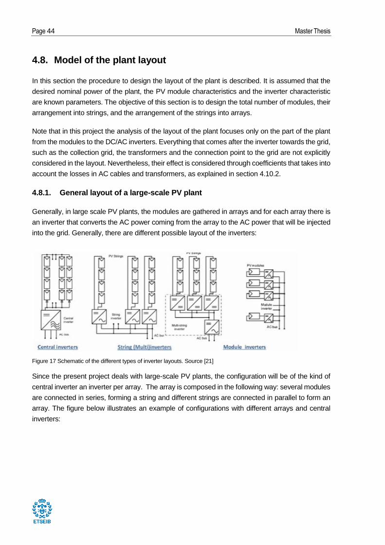
Page 44 Master Thesis
4.8. Model of the plant layout
In this section the procedure to design the layout of the plant is described. It is assumed that the
desired nominal power of the plant, the PV module characteristics and the inverter characteristic
are known parameters. The objective of this section is to design the total number of modules, their
arrangement into strings, and the arrangement of the strings into arrays.
Note that in this project the analysis of the layout of the plant focuses only on the part of the plant
from the modules to the DC/AC inverters. Everything that comes after the inverter towards the grid,
such as the collection grid, the transformers and the connection point to the grid are not explicitly
considered in the layout. Nevertheless, their effect is considered through coefficients that takes into
account the losses in AC cables and transformers, as explained in section 4.10.2.
4.8.1. General layout of a large-scale PV plant
Generally, in large scale PV plants, the modules are gathered in arrays and for each array there is
an inverter that converts the AC power coming from the array to the AC power that will be injected
into the grid. Generally, there are different possible layout of the inverters:
Figure 17 Schematic of the different types of inverter layouts. Source [21]
Since the present project deals with large-scale PV plants, the configuration will be of the kind of
central inverter an inverter per array. The array is composed in the following way: several modules
are connected in series, forming a string and different strings are connected in parallel to form an
array. The figure below illustrates an example of configurations with different arrays and central
inverters:
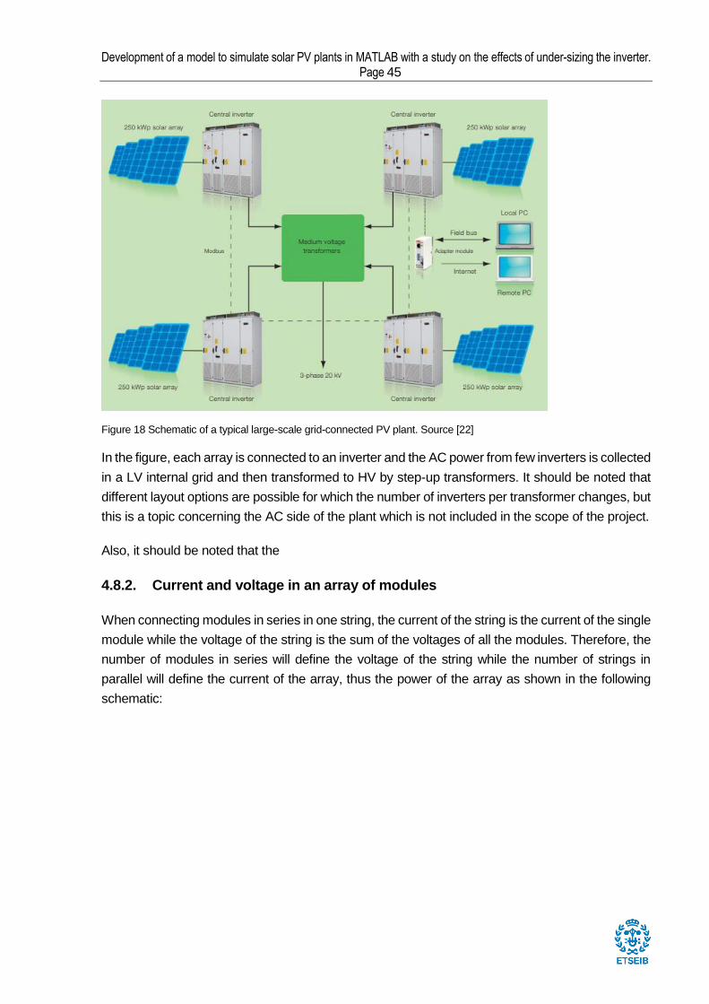
Development of a model to simulate solar PV plants in MATLAB with a study on the effects of under-sizing the inverter. Page 45
Figure 18 Schematic of a typical large-scale grid-connected PV plant. Source [22]
In the figure, each array is connected to an inverter and the AC power from few inverters is collected
in a LV internal grid and then transformed to HV by step-up transformers. It should be noted that
different layout options are possible for which the number of inverters per transformer changes, but
this is a topic concerning the AC side of the plant which is not included in the scope of the project.
Also, it should be noted that the
4.8.2. Current and voltage in an array of modules
When connecting modules in series in one string, the current of the string is the current of the single
module while the voltage of the string is the sum of the voltages of all the modules. Therefore, the
number of modules in series will define the voltage of the string while the number of strings in
parallel will define the current of the array, thus the power of the array as shown in the following
schematic:
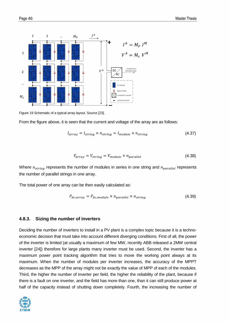
Page 46 Master Thesis
Figure 19 Schematic of a typical array layout. Source [23].
From the figure above, it is seen that the current and voltage of the array are as follows:
𝐼𝑎𝑟𝑟𝑎𝑦 = 𝐼𝑠𝑡𝑟𝑖𝑛𝑔 × 𝑛𝑠𝑡𝑟𝑖𝑛𝑔 = 𝐼𝑚𝑜𝑑𝑢𝑙𝑒 × 𝑛𝑠𝑡𝑟𝑖𝑛𝑔 (4.37)
𝑉𝑎𝑟𝑟𝑎𝑦 = 𝑉𝑠𝑡𝑟𝑖𝑛𝑔 = 𝑉𝑚𝑜𝑑𝑢𝑙𝑒 × 𝑛𝑝𝑎𝑟𝑎𝑙𝑙𝑒𝑙 (4.38)
Where 𝑛𝑠𝑡𝑟𝑖𝑛𝑔 represents the number of modules in series in one string and 𝑛𝑝𝑎𝑟𝑎𝑙𝑙𝑒𝑙 represents
the number of parallel strings in one array.
The total power of one array can be then easily calculated as:
𝑃𝑑𝑐,𝑎𝑟𝑟𝑎𝑦 = 𝑃𝑑𝑐,𝑚𝑜𝑑𝑢𝑙𝑒 × 𝑛𝑝𝑎𝑟𝑎𝑙𝑙𝑒𝑙 × 𝑛𝑠𝑡𝑟𝑖𝑛𝑔 (4.39)
4.8.3. Sizing the number of inverters
Deciding the number of inverters to install in a PV plant is a complex topic because it is a techno-
economic decision that must take into account different diverging conditions. First of all, the power
of the inverter is limited (at usually a maximum of few MW, recently ABB released a 2MW central
inverter [24]) therefore for large plants many inverter must be used. Second, the inverter has a
maximum power point tracking algorithm that tries to move the working point always at its
maximum. When the number of modules per inverter increases, the accuracy of the MPPT
decreases as the MPP of the array might not be exactly the value of MPP of each of the modules.
Third, the higher the number of inverter per field, the higher the reliability of the plant, because if
there is a fault on one inverter, and the field has more than one, than it can still produce power at
half of the capacity instead of shutting down completely. Fourth, the increasing the number of
Development of a model to simulate solar PV plants in MATLAB with a study on the effects of under-sizing the inverter. Page 47
inverter might (or might not) increase the costs. These are among the main reasons that would pull
the decisions either to increase or decrease the number of inverter. A thorough analysis that does
an optimization of different techno-economic parameters, would probably require another entire
project and is out of the scope of the present work.
Therefore, the strategy for the design of the number of the inverters is simplified in two steps. Firstly,
the user chooses an inverter model and given a desired power the number of the inverters is
calculated by:
𝑛𝑖𝑛𝑣𝑒𝑟𝑡𝑒𝑟𝑠 = 𝑛𝑎𝑟𝑟𝑎𝑦 =𝑃𝑑𝑐,𝑓𝑖𝑒𝑙𝑑
𝑃𝑎𝑐,𝑖𝑛𝑣𝑒𝑟𝑡𝑒𝑟𝜂𝑖𝑛𝑣 (4.40)
Where 𝑃𝑑𝑐,𝑓𝑖𝑒𝑙𝑑 is the nominal DC power of the plant in W, 𝑃𝑎𝑐,𝑖𝑛𝑣𝑒𝑟𝑡𝑒𝑟 is the nominal AC power of
the inverter and 𝜂𝑖𝑛𝑣 is the nominal efficiency of the inverter.
Secondly, the program outputs the DC-to-AC ratio calculated as:
𝐷𝐶/𝐴𝐶 =𝑃𝑑𝑐,𝑎𝑟𝑟𝑎𝑦
𝑃𝑎𝑐,𝑖𝑛𝑣𝑒𝑟𝑡𝑒𝑟 (4.41)
With the DC-to-AC ratio and the clipping losses, the designer can either increase or decrease the
size or number of inverters as discussed in Section 6.2 . This strategy is taken from PVsyst in which
the inverter selects an inverter and a desired power and the program warns if the specific design
produces high clipping losses[8].
4.8.4. Sizing the number of modules in series
To size the number of modules in a string, the limits on the voltage are applied. Since the number
of modules in series will define the voltage of the string and thus the voltage of the array, this
number is designed in order to respect the limits on the voltage imposed by the inverter MPPT and
by the maximum voltage allowable in inverter and modules. These conditions translate into 4
inequalities as follows.
The voltage of the array must always be inside the operating range of the MPPT of the inverter:
𝑉𝑎𝑟𝑟𝑎𝑦,𝑚𝑝𝑝,𝑚𝑖𝑛 > 𝑉𝑖𝑛𝑣,𝑚𝑝𝑝𝑡,𝑚𝑖𝑛 (4.42)
𝑉𝑎𝑟𝑟𝑎𝑦,𝑚𝑝𝑝,𝑚𝑎𝑥 < 𝑉𝑖𝑛𝑣,𝑚𝑝𝑝𝑡,𝑚𝑎𝑥 (4.43)
The absolute maximum voltage of the array must be lower than the maximum allowable voltage of
the inverter and of the module:

Page 48 Master Thesis
𝑉𝑎𝑟𝑟𝑎𝑦,𝑂𝐶,𝑚𝑎𝑥 < 𝑉𝑖𝑛𝑣,𝑖𝑛𝑝𝑢𝑡,𝑚𝑎𝑥 (4.44)
𝑉𝑎𝑟𝑟𝑎𝑦,𝑂𝐶,𝑚𝑎𝑥 < 𝑉𝑚𝑜𝑑𝑢𝑙𝑒,𝑠𝑦𝑠𝑡𝑒𝑚,𝑚𝑎𝑥 (4.45)
The range for MPPT, the maximum voltage of the inverter and of the panels are known as always
present in the datasheets of the components. In addition, for these four conditions, three voltages
of the PV module need to be known: the maximum and minimum operating voltages and the
minimum absolute open circuit voltage. By default, the program calculates them with the single
diode model of the IV curve, calculating the curve at different temperatures.
It should be noted that while the single diode model is built to be precise on the maximum power
point, its accuracy on the open circuit voltage should be discussed. That is why in the designing
phase, to calculate the Voc at minimum temperature, the program allows to use the single diode
model or directly the temperature coefficient of Voc that is usually provided by manufacturers. The
choice of one or the other is left to the user of the program. The values calculated with the two
methods could lead to different values and therefore to different maximum limit for the number of
modules in series. This is because in the default version of the single diode model (see section
4.6.3) the value of muVoc is not used to build the model, therefore the muVoc of the model might
be slightly different from the value of the manufacturers. However, this does not affect the energy
yield as the power is produced at Vmpp and not at Voc. This line of reasoning and the possibility
of choosing either one of the method are taken from the manual of PVsyst that discusses the topic
in further details [8]. In PVsyst, the default is to calculate the maximum open circuit voltage with the
single diode model, and this approach was followed in the present work.
The default design temperatures are set to the default values of PVsyst:
𝑇𝑚𝑎𝑥,𝑜𝑝𝑒𝑟𝑎𝑡𝑖𝑛𝑔 = 60 °𝐶 (4.46)
𝑇𝑚𝑖𝑛,𝑜𝑝𝑒𝑟𝑎𝑡𝑖𝑛𝑔 = 20 °𝐶 (4.47)
𝑇𝑚𝑖𝑛,𝑎𝑏𝑠𝑜𝑙𝑢𝑡𝑒 = −10 °𝐶 (4.48)
Anyway, they can be changed in the parameters of the model.
Once the temperatures are defined and the way to find the desinging Voc is set, the software
computes simultaneously all the conditions listed above and finds a range of possible numbers of
modules in series.

Development of a model to simulate solar PV plants in MATLAB with a study on the effects of under-sizing the inverter. Page 49
4.8.5. Sizing the number of strings in parallel
The sizing of the number of strings per array is performed starting from the power of the strings.
For each of the possible string arrangements found in section 4.8.4, the number of strings is found
by respecting simultaneously the two following conditions:
𝑛𝑠𝑡𝑟𝑖𝑛𝑔𝑠 =𝑃𝑎𝑟𝑟𝑎𝑦,𝐷𝐶
𝑃𝑠𝑡𝑟𝑖𝑛𝑔,𝐷𝐶 (4.49)
Or equivalently:
𝑛𝑠𝑡𝑟𝑖𝑛𝑔𝑠 =𝑛𝑚𝑜𝑑𝑢𝑙𝑒𝑠,𝑎𝑟𝑟𝑎𝑦
𝑛𝑚𝑜𝑑𝑢𝑙𝑒𝑠,𝑠𝑡𝑟𝑖𝑛𝑔 (4.50)
And:
𝐼𝑚𝑜𝑑𝑢𝑙𝑒,𝑚𝑎𝑥𝑛𝑠𝑡𝑟𝑖𝑛𝑔𝑠 ≤ 𝐼𝑖𝑛𝑣𝑒𝑟𝑡𝑒𝑟,𝑚𝑎𝑥 (4.51)
The first condition is needed to reach the desired power, while the second condition must be verified
to comply with the technical limits of the inverter. This means that if the second condition is
respected, for each of the possible number of modules in series there is a configuration with its
number of strings in parallel, otherwise the configuration is not possible.
4.8.6. The possible configurations and designs of the array voltage
Once the inverter was sized, and the different configurations of number of modules in series and in
parallel were calculates, a table that sums up the possible configurations and additional details
(such as array voltage and current range etc.) is created:
Table 1: Typical table of possible layout configurations
Variable Opt.1 Opt.2 Opt.3
N series 15 16 17
N parallel 309 290 273
Vmin 492 524 557
Vmax 576 614 652
DC Power (W) 1483867 1485468 1485788
AC Power (W) 1447030 1448591 1448903
Total modules 4635 4640 4641
All of the configurations generated are possible configurations that respect all the limit discussed in
sections 4.8.4 and 4.8.5. However, for the final design, only one configuration must be chosen. The
choice of the configuration is usually based on the voltage range of the particular configuration as
this will affect the losses of the plant. The choice is not trivial because with a higher voltage, the

Page 50 Master Thesis
losses of the inverter increase while the losses of the DC cables decrease. Moreover, a third factor
could be considered because the current of a string is determined by the module with the lowest
current, which means that in case one of the modules in a string performs badly (because of soiling,
hotspots, technical issues etc.) the current of the whole string is affected. For this last reason, a
lower number of modules in string should increase the reliability of the plant. Even disregarding this
last consideration, the two first conditions pulls towards two different directions therefore a tradeoff
must be found. A detailed optimization is not performed in the present project and a configuration
on the middle is usually chosen as default.
4.9. Model of the inverter
In this section the relationship between the inverter input power in DC and the inverter output AC
power is presented. In the present project the inverter is considered as a black box and the it models
only the transfer function between the inputs and the output, which is the efficiency which is the
same as in PVsyst and in SAM. The algorithm to model the inverter is taken from SAM, because
an explicit algorithm from PVsyst could not be found.
4.9.1. The Sandia inverter model with empirical coefficients
The algorithm proposed by SAM [9] is based on a study in which the behavior of the inverter is
modelled through four experimental parameters [25]. The relationship between DC power and AC
power reads as follows:
𝑃𝑎𝑐 = [𝑃𝑎𝑐,0𝐴 − 𝐵
− 𝐶(𝐴 − 𝐵)] (𝑃𝑑𝑐 − 𝐵) + 𝐶(𝑃𝑑𝑐 −𝐵)2 (4.52)
Where:
𝐴 = 𝑃𝑑𝑐[1 + 𝐶1(𝑉𝑑𝑐 − 𝑉𝑑𝑐,0)] (4.53)
𝐵 = 𝑃𝑠𝑜[1 + 𝐶2(𝑉𝑑𝑐 − 𝑉𝑑𝑐,0)] (4.54)
𝐶 = 𝐶0[1 + 𝐶3(𝑉𝑑𝑐 − 𝑉𝑑𝑐,0)] (4.55)
Where the variables are: Pac is the AC power output of the inverter, Pdc is the DC power input of the inverter, Vdc is the DC voltage input of the inverter
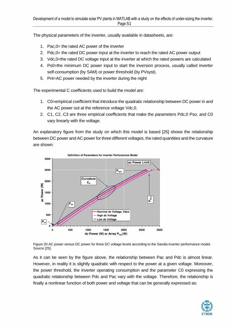
Development of a model to simulate solar PV plants in MATLAB with a study on the effects of under-sizing the inverter. Page 51
The physical parameters of the inverter, usually available in datasheets, are:
1. Pac,0= the rated AC power of the inverter
2. Pdc,0= the rated DC power input at the inverter to reach the rated AC power output
3. Vdc,0=the rated DC voltage input at the inverter at which the rated powers are calculated
4. Ps0=the minimum DC power input to start the inversion process, usually called inverter
self-consumption (by SAM) or power threshold (by PVsyst).
5. Pnt=AC power needed by the inverter during the night
The experimental C coefficients used to build the model are:
1. C0=empirical coefficient that introduce the quadratic relationship between DC power in and
the AC power out at the reference voltage Vdc,0.
2. C1, C2, C3 are three empirical coefficients that make the parameters Pdc,0 Pso, and C0
vary linearly with the voltage.
An explanatory figure from the study on which this model is based [25] shows the relationship
between DC power and AC power for three different voltages, the rated quantities and the curvature
are shown:
Figure 20 AC power versus DC power for three DC voltage levels according to the Sandia inverter performance model. Source [25].
As it can be seen by the figure above, the relationship between Pac and Pdc is almost linear.
However, in reality it is slightly quadratic with respect to the power at a given voltage. Moreover,
the power threshold, the inverter operating consumption and the parameter C0 expressing the
quadratic relationship between Pdc and Pac vary with the voltage. Therefore, the relationship is
finally a nonlinear function of both power and voltage that can be generally expressed as:
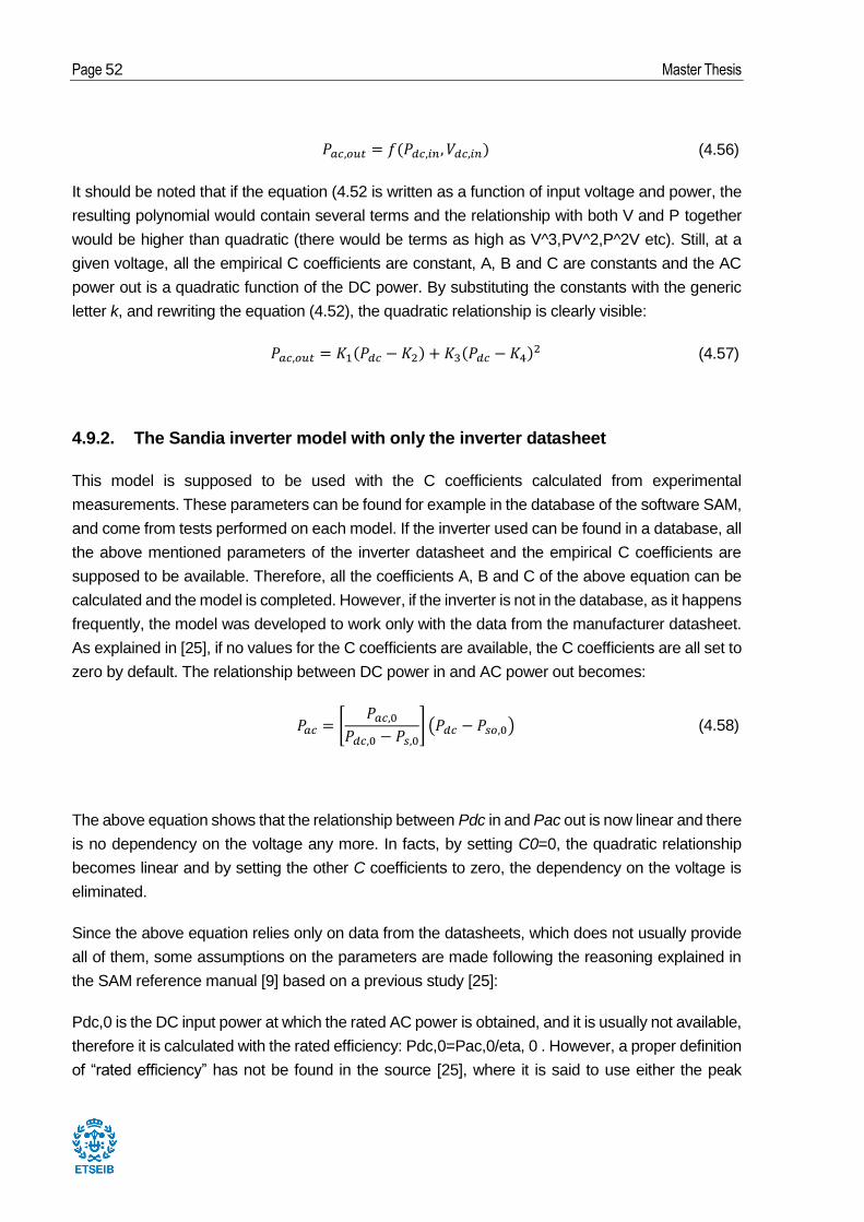
Page 52 Master Thesis
𝑃𝑎𝑐,𝑜𝑢𝑡 = 𝑓(𝑃𝑑𝑐,𝑖𝑛, 𝑉𝑑𝑐,𝑖𝑛) (4.56)
It should be noted that if the equation (4.52 is written as a function of input voltage and power, the
resulting polynomial would contain several terms and the relationship with both V and P together
would be higher than quadratic (there would be terms as high as V^3,PV^2,P^2V etc). Still, at a
given voltage, all the empirical C coefficients are constant, A, B and C are constants and the AC
power out is a quadratic function of the DC power. By substituting the constants with the generic
letter k, and rewriting the equation (4.52), the quadratic relationship is clearly visible:
𝑃𝑎𝑐,𝑜𝑢𝑡 = 𝐾1(𝑃𝑑𝑐 − 𝐾2) + 𝐾3(𝑃𝑑𝑐 − 𝐾4)2 (4.57)
4.9.2. The Sandia inverter model with only the inverter datasheet
This model is supposed to be used with the C coefficients calculated from experimental
measurements. These parameters can be found for example in the database of the software SAM,
and come from tests performed on each model. If the inverter used can be found in a database, all
the above mentioned parameters of the inverter datasheet and the empirical C coefficients are
supposed to be available. Therefore, all the coefficients A, B and C of the above equation can be
calculated and the model is completed. However, if the inverter is not in the database, as it happens
frequently, the model was developed to work only with the data from the manufacturer datasheet.
As explained in [25], if no values for the C coefficients are available, the C coefficients are all set to
zero by default. The relationship between DC power in and AC power out becomes:
𝑃𝑎𝑐 = [𝑃𝑎𝑐,0
𝑃𝑑𝑐,0 − 𝑃𝑠,0] (𝑃𝑑𝑐 − 𝑃𝑠𝑜,0) (4.58)
The above equation shows that the relationship between Pdc in and Pac out is now linear and there
is no dependency on the voltage any more. In facts, by setting C0=0, the quadratic relationship
becomes linear and by setting the other C coefficients to zero, the dependency on the voltage is
eliminated.
Since the above equation relies only on data from the datasheets, which does not usually provide
all of them, some assumptions on the parameters are made following the reasoning explained in
the SAM reference manual [9] based on a previous study [25]:
Pdc,0 is the DC input power at which the rated AC power is obtained, and it is usually not available,
therefore it is calculated with the rated efficiency: Pdc,0=Pac,0/eta, 0 . However, a proper definition
of “rated efficiency” has not be found in the source [25], where it is said to use either the peak

Development of a model to simulate solar PV plants in MATLAB with a study on the effects of under-sizing the inverter. Page 53
efficiency or the CEC/EU efficiency. Therefore, the CEC or EU efficiency will be used in the present
work, and if not available, the maximum efficiency will be used instead. The weighted efficiency is
chosen as the first choice because PV inverter usually do not reach their maximum efficiency at
rated power, but instead at lower power as explained in the note at the end of the section.
Pso,0 is the DC input power needed to start the conversion (also called inverter self-consumption)
and if not available from the inverter datasheet, it is assumed to be 1% of the rated DC power Pdc,0
as advised in [25].
Pac0 is the rated AC power of the inverter, which is always available.
It should be noted that the setting C0=0 in the above equation, the relationship between Pdc in and
Pac out becomes linear, and if the efficiency is calculated as Pacout/ Pdcin:
𝜂𝑖𝑛𝑣 =𝑃𝑎𝑐,0
𝑃𝑑𝑐,0 − 𝑃𝑠,0(1 −
𝑃𝑠,0𝑃𝑑𝑐
) (4.59)
It can be noted that the efficiency increases when Pdc in increases, which means that at maximum
power in there is the maximum of the efficiency. However, as already said above, this is usually not
the case for PV inverters where the maximum is somewhere around 60% of the rated dc power as
suggested by PVsyst [8] or 50% as suggested by the authors of a study that compares different
modelling approaches [26]. This paper suggested that even without the empirical coefficients, the
value of C0 should be set to a default so that the quadratic behavior is preserved. The authors
suggest that the default value of C0 could be taken assuming that the known maximum efficiency
occurs when Pdc,in =50%. Even though this approach might increase the accuracy, in the present
work it has not been applied, because it was preferred to follow the original Sandia model, which
does not include it.
4.9.3. Night consumption and power clipping
The SANDIA inverter model applies the following limits to the power input and output:
At night, when clearly Pdc=0, the inverter power output Pac=-Pnight, because the inverter needs
power to stay on and sense if some power from the PV panels is received. However, in the present
model, this option can be deactivated and night consumption set to zero, because theoretically the
inverter could be switched off during nighttime, and switched on before the sun rises.
During the day, if Pdc<Pso then the inverter power Pac=-Pnight. This check is always activated
because during the day the inverter is effectively always on.
During the day if Pdc>Pdc,0 then the inverter output power is set to Pac= Pac,0. The inverter clips
the power in excess by changing the operating point of the I-V curve away from its maximum. The
clipped power is stored in a vector as it might be needed for analysis, for example in the study case
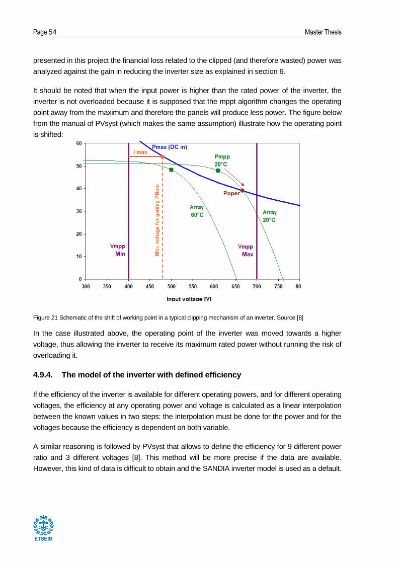
Page 54 Master Thesis
presented in this project the financial loss related to the clipped (and therefore wasted) power was
analyzed against the gain in reducing the inverter size as explained in section 6.
It should be noted that when the input power is higher than the rated power of the inverter, the
inverter is not overloaded because it is supposed that the mppt algorithm changes the operating
point away from the maximum and therefore the panels will produce less power. The figure below
from the manual of PVsyst (which makes the same assumption) illustrate how the operating point
is shifted:
Figure 21 Schematic of the shift of working point in a typical clipping mechanism of an inverter. Source [8]
In the case illustrated above, the operating point of the inverter was moved towards a higher
voltage, thus allowing the inverter to receive its maximum rated power without running the risk of
overloading it.
4.9.4. The model of the inverter with defined efficiency
If the efficiency of the inverter is available for different operating powers, and for different operating
voltages, the efficiency at any operating power and voltage is calculated as a linear interpolation
between the known values in two steps: the interpolation must be done for the power and for the
voltages because the efficiency is dependent on both variable.
A similar reasoning is followed by PVsyst that allows to define the efficiency for 9 different power
ratio and 3 different voltages [8]. This method will be more precise if the data are available.
However, this kind of data is difficult to obtain and the SANDIA inverter model is used as a default.
Development of a model to simulate solar PV plants in MATLAB with a study on the effects of under-sizing the inverter. Page 55
4.10. Model of the losses of the plant
This section introduces the losses of the plant that have not explicitly been considered in other
sections. These losses are the DC cable losses and the AC cable and transformer losses. Optical
losses are treated in section 4.5, effects of the temperature are treated in section 4.7, and inverter
losses are treated in section 4.9.
4.10.1. DC cabling losses
To calculate the DC cabling losses, in theory a detailed analysis with sizing of the different sections
of the cables is needed. However, in the present project, a simpler approach is used that allows to
consider a first approximation of the DC losses of the plants without having to perform a detailed
design of the cables. This approach is taken from the first approximation approach used by PVsyst
in treating DC losses. PVsyst also offers a specific tool to effectively model the cable losses in a
precise way. However, this second approach has not been implemented in the present project for
the sake of simplicity, but could certainly be an interesting further development.
The first approximation used by PVsyst calculates the DC losses is performed by setting a specific
resistance of the wire as a percentage of the standard resistance of the array, in three steps. Firstly,
the standard resistance of the array is calculated as voltage over current of the array. Secondly,
the resistance of the wires is set to a percentage of the standard resistance of the array. Thirdly,
the ohmic losses of the cables are calculated with the resistance of the wires and the current of the
array. The three steps can be summarized as:
Calculated once per simulation:
𝑅𝑎𝑟𝑟𝑎𝑦 =𝑉𝑎𝑟𝑟𝑎𝑦,𝑆𝑇𝐶
𝐼𝑎𝑟𝑟𝑎𝑦,𝑆𝑇𝐶 (4.60)
𝑅𝑑𝑐,𝑤𝑖𝑟𝑖𝑛𝑔 = 𝑅𝑎𝑟𝑟𝑎𝑦𝑃𝑙𝑜𝑠𝑠,𝑆𝑇𝐶 (4.61)
Calculated every hour:
𝑃𝑙𝑜𝑠𝑠,𝑑𝑐,𝑐𝑎𝑏𝑙𝑒𝑠 = 𝑅𝑑𝑐,𝑤𝑖𝑟𝑖𝑛𝑔𝐼𝑎𝑟𝑟𝑎𝑦2 (4.62)
With the above equation, it is possible to calculate a first approximation of the DC losses of the
plant by only using one parameter. The percentage of 𝑅𝑑𝑐,𝑤𝑖𝑟𝑖𝑛𝑔 with respect to 𝑅𝑎𝑟𝑟𝑎𝑦 is set to
1.5% by default following the default value of PVsyst. This parameter can anyway be modified at
any simulation.
Although this approach is a first approximation, it is nevertheless already an improvement with

Page 56 Master Thesis
respect to models that calculate only a yearly percentage loss. Because it allows the loss to vary
with the current, therefore for example it can be an indicator to choose the specific configuration of
the layout of the plant as described in 4.8.6.
It should be noted that to avoid large amount of losses in the DC cables transporting power to the
main AC inverters, it is usually good practice to put many panels in series so that the voltage is
increased while the current is kept at the value of one single module. While lowering the DC losses,
this method could lead to high mismatch losses because the current is limited by the lowest current
in a string, and if one panel in a string is performing badly, it will affect all the others [4].
4.10.2. AC cabling and transformer losses
The AC cable losses and the transformer losses are considered only through a yearly percentage
loss factor. This is the default method used in SAM (also for DC cables). PVsyst instead offers a
more detailed approach in which the cables and transformers are modeled. However, this last
approach has not been followed for the sake of simplicity, but could be an interesting further
development. In the present model, the losses are expressed as:
𝜂𝑎𝑐,𝑐𝑎𝑏𝑙𝑒𝑠 = 1 − 𝐿𝑎𝑐,𝑐𝑎𝑏𝑙𝑒𝑠 (4.63)
𝜂𝑎𝑐,𝑡𝑟𝑎𝑛𝑠𝑓𝑜𝑟𝑚𝑒𝑟 = 1 − 𝐿𝑎𝑐,𝑡𝑟𝑎𝑛𝑠𝑓𝑜𝑟𝑚𝑒𝑟 (4.64)
The default values of losses are both set to 1% and can be modified at any moment.

Development of a model to simulate solar PV plants in MATLAB with a study on the effects of under-sizing the inverter. Page 57
4.11. Model of the energy yield
This section introduces the procedure followed to calculate the hourly and yearly energy injected
to the grid. It supposes that the energy output from the arrays is already computed hourly (see
section 4.8.2). Since in the program the time step at which power is calculated is one hour, and the
energy is expressed as kWh, the value of energy and power are the same at a given hour.
The power flow can be summarized in five steps. First, the global horizontal irradiance arriving
from the sun is adjusted to calculate the effective POA irradiance that hits the cells, introducing
losses related to the tilt of the panel and optical losses. Second, the energy arriving from the sun
is transformed by the modules in electric energy trough the photovoltaic effect which is modeled
by the single diode model (see section 4.6). Third, the DC energy is collected at each array with
DC cables that introduce ohmic losses (see section 4.10.1). Fourth, the DC power coming from
the arrays is converted to AC power by the inverters, introducing the inverter losses modeled in
section 4.9. Fifth, the AC power output from the inverter is transported to the point of connection
to the grid passing through AC cables and step up transformers, introducing losses described in
4.10.2. Finally, the energy yield injected to the grid can be calculated as:
𝐸𝑔𝑟𝑖𝑑,ℎ𝑜𝑢𝑟𝑙𝑦 =∑ (𝐸𝑎𝑐,𝑖𝑛𝑣,𝑜𝑢𝑡,𝑖 )𝑛_𝑖𝑛𝑣𝑒𝑟𝑡𝑒𝑟
𝑖=1𝜂𝑎𝑐,𝑐𝑎𝑏𝑙𝑒𝑠 𝜂𝑎𝑐,𝑡𝑟𝑎𝑛𝑠𝑓𝑜𝑟𝑚𝑒𝑟 (4.65)
Where: 𝜂𝑎𝑐,𝑡𝑟𝑎𝑛𝑠𝑓𝑜𝑟𝑚𝑒𝑟 and 𝜂𝑎𝑐,𝑐𝑎𝑏𝑙𝑒𝑠 cables are the efficiencies of transformers and AC cables
(see section 4.10.2).
The software calculates all the variables hourly, and by simply summing all the values over one
year, the yearly energy output can be computed as:
𝐸𝑔𝑟𝑖𝑑,𝑦𝑒𝑎𝑟𝑙𝑦 = ∑ 𝐸𝑔𝑟𝑖𝑑,ℎ𝑜𝑢𝑟𝑙𝑦 𝐹𝑎𝑣𝑎𝑖𝑙𝑎𝑖𝑏𝑖𝑙𝑖𝑡𝑦
8760
1
(4.66)
Availability is an additional optional parameter that is used to take into account that the plant
might be unavailable during certain hours of the year, as done by SAM [9].

Page 58 Master Thesis
4.12. Model of the LCOE
When assessing costs and the economic feasibility of a technology in electrical power generation,
one of the most important indicator is the levelized cost of electricity (LCOE). The LCOE is a way
to express what is the cost of producing one unit of energy (Kwh) with a particular technology. It
calculates all the costs needed during the lifetime of the project and divide them by the total amount
of energy that the project is expected to produce. The LCOE can also be thought as the minimum
price at which electricity should be sold to reach the desired return on investment. The LCOE is a
very important indicator as it can be used to compare different technologies with different lifetime,
different fuels, different energy production, different costs etc.
The formula used in this project to calculate the LCOE is taken from the methodology of the
International Renewable Energy Agency (IRENA) [27] :
𝐿𝐶𝑂𝐸 =∑
𝐼𝑡 +𝑀𝑡 + 𝐹𝑡(1 + 𝑟)𝑡
𝑛𝑡=1
∑𝐸𝑡
(1 + 𝑟)𝑡𝑛𝑡=1
(4.67)
Where: 𝐼𝑡 represents all the investments in year t, 𝑀𝑡 represents all the operations and
maintenance expenditures (O&M) in the year t, 𝐹𝑡 represents all the fuel expenditures in year t, 𝐸𝑡
is the electricity generation in year t, 𝑟 is the discount rate and 𝑛 is the life of the system.
The nominator is the present value of all costs of the plants during its lifetime and the denominator
is the present value of all the electricity produced over the lifetime of the project.
In this project the generalized form can be further simplified with the following assumptions:
1. The sun is free: there are no fuel expenditures
2. The investments are considered to be performed at year 0, beginning of the project: CAPEX
is out of the sum in the nominator.
3. The discount rate is the weighted average cost of capital or WACC (see below)
4. The yearly production is affected by the degradation of the panels, and it can be expressed
as linear degradation or percentage decrease (D).
5. The residual value of the system is considered to be zero.
Therefore the formula can be re-written as the typical formula used in the solar industry [28]:

Development of a model to simulate solar PV plants in MATLAB with a study on the effects of under-sizing the inverter. Page 59
𝐿𝐶𝑂𝐸 =𝐶𝐴𝑃𝐸𝑋 + ∑
𝑂𝑃𝐸𝑋(1 +𝑊𝐴𝐶𝐶)𝑡
𝑛𝑡=1
∑𝑌0(1 − 𝐷)
𝑛
(1 +𝑊𝐴𝐶𝐶)𝑡𝑛𝑡=1
(4.68)
The CAPEX represent all the investments that were made at the beginning of the project such as
costs of the modules, inverters, cabling etc. (a detailed cost breakdown is presented in section
6.3.2.1). The OPEX represents all the yearly costs needed for the operation and maintenance of
the plant.
The discount rate that is usually used when analyzing renewable energy projects is the weighted
average cost of capital: it is a weighted average of the expected rate of return of the various
investors. RES projects frequently involve financing from equity and debt. There might be different
equity/debt ratio and the different parties could have different expectations for the return on
investment. Therefore, the WACC weights differently the discounts rates of the two parties. WACC
is given by::
𝑊𝐴𝐶𝐶 = 𝐸𝑞%𝐼𝑅𝑅% +𝐷𝑒𝑏𝑡%𝑖𝑑𝑒𝑏𝑡(1 − 𝑇𝑐𝑜𝑟𝑝) (4.69)
Where: 𝐸𝑞% is the percentage of CAPEX that is equity, 𝐼𝑅𝑅% is the expected Internal rate of return
of the equity financiers or cost of equity, 𝐷𝑒𝑏𝑡% is the percentage of CAPEX that is debt, 𝑖𝑑𝑒𝑏𝑡 is
the interest rate of the debt, or expected Internal rate of return of the debt financiers or cost of debt
and 𝑇𝑐𝑜𝑟𝑝 is the corporate tax rate.
Note that the corporate tax rate is included in the formula because the annual interest on a debt is
tax deductible. This is among the reasons why debt financing is an interesting option for large
projects: if the cost of equity and debt are the same, it could be more convenient to increase the
debt percentage. In facts, thanks to tax deductions, a higher debt percentage would overall reduce
the WACC.
In this project the LCOE was calculated with the formula expressed above as it is the general
simplified formula that agencies like IRENA use [27].
More complex approaches can be used, such as the one used by Lazard [29] in which the all the
financials variables are calculated separately for each year, and the LCOE is found as the selling
price of electricity that allows to obtain the desired IRR. However, the simplified approach used in
this project is detailed enough as the value of WACC can be found in literature and the results can
be easily compared with the ones of most of the agencies using the same approach (such as
IRENA, etc).
Since LCOE can be though as of the minimum price at which electricity should be sold to reach the
desired WACC, the higher the WACC the higher the LCOE. Moreover, the WACC is country
dependent, and can change case by case [30].

Page 60 Master Thesis
5. Validation of the models
In this section the validation of the model developed is described in two parts: first, each sub model
is tested separately with the same input of the sub model and then an overall validation of the whole
model is presented. Usually, when validating a model, the results of a simulation are compared
with measured data to see the accuracy of the prediction of the model. However, in the present
project the validation is performed against result coming from PVsyst or eventually from SAM,
because the technical equipment to test real scenarios was not available and accurate
measurements would have required measurements of parameters for a long time (even several
years) which could have not been done.
Since PVsyst was used as a reference and it is trusted by the industry as discussed in Section 4.1
results of the present project are considered satisfactory if they get close to the ones of PVsyst.
PVsyst, was developed during years and several validations of this software are available, for
example from [8].
To perform the validation, the hourly values of the output file from the code written in the present
project and the output file from the advanced simulation done in PVsyst are compared.
5.1. Validation of the complete model
During the development of this model, a validation was performed for each sub-model, both
software run with exactly the same inputs, and the outputs are compared, so that the results were
not affected by discrepancies in the inputs (that might come from a previous model). However, in
a real simulation, the inputs of the model are introduced only once, and each sub model has as
inputs the outputs of the previous sub model which already contain an error, therefore the overall
error will be amplified. In this section the whole simulation is tested starting from the same weather
file, module and inverter. Clearly, in PVsyst and in the software developed all the parameters that
should be assumed are set at the same values (e.g. the heat transfer coefficient, the albedo etc.).
The following table summarizes the results of the validation, performed with the 1 MW plant using
the same inverter and module of the case study (Section 6.3.1) a with a weather file synthetically
generated in Barcelona (the accuracy of the file is not important as it will just serve as the input for
both software).

Development of a model to simulate solar PV plants in MATLAB with a study on the effects of under-sizing the inverter. Page 61
Table 2 Validation RMSE and MBD for four main variables
Sub-Model RMSE MBD Reference Model
Global Effective 0.15% 0.046% PVsyst
Cell Temp. Heat transfer 0. 08% 0.022% PVsyst
DC power 0.27% 0.074% PVsyst
As it can be seen from both the table the RMSE for DC power is 0.27%, and since the accuracy of
PVsyst is around 1% if compared with measured data, it is considered a very positive and
satisfactory result, because it means that given a weather file, both models will predict the hourly
energy output with an error below 1%.

Page 62 Master Thesis
6. Case Study: the effect of under sizing the inverter
In this section, a case study on the economic effects of under sizing the inverter on the LCOE and
CAPEX of the plant is presented.
6.1. Case study objective
The study case analyses the effects of under-sizing the inverter on the LCOE of the plant. When
designing a PV power plant, it is important to know the DC nominal power of the solar field and to
carefully select the AC rated power of the inverters. Since solar panels produce the nameplate
power only under standard conditions of G=1000W and T=25 degrees, and these conditions
happen only few times during the year, the solar field will almost always produce less than its
nominal capacity, therefore the inverter could be smaller than the solar field. The ratio of the DC
power of the solar array to the AC power of the inverter is called DC-to-AC ratio. The relationship
between the LCOE of the plant and the DC-to-AC ratio will be studied in the next sections with the
objective of finding the DC-to-AC ratio that minimizes the LCOE.
The problem is known to the solar industry, and different studies were performed on the topic from
different points of view, such as [31] that analyses the financial effects or [32] that analyses the
impact on the reliability of the inverter. Many deal with the financial effects of under sizing the
inverter but generally the conclusions are drawn always for generic location. The purpose of this
case study is instead to quantitatively relate the quality of the irradiance to the best DC-to-AC ratio.
As a result, just only analyzing the weather file, one could be able to have a general guideline on
the size of the inverter.
This case study is an interesting application where the software developed in the present project is
particularly useful. The software has a specific model for the technical performance and the LCOE
model, and can run in loops by changing the sizing parameters at every simulation. Therefore, it
can output results for different locations with different sizing with just one run. Moreover, the ability
of the software to work with hourly variables is crucial as the study of energy losses due to clipping
and energy gains due to higher efficiency of the inverter would not be possible without hourly
values.
6.2. Case study methodology
In different locations the effect of changing the DC-to-AC ratio was studied. The variables analyzed
are LCOE, the CAPEX and the capacity factor of the plant. For all the simulations, the model of the
inverter, the module and all the modelling parameters and the financial assumptions are the same.
For each location, the study was performed in four step. First, a weather file was selected for the
particular location. Second, the technical simulation runs for different DC-to-AC ratios and outputs

Development of a model to simulate solar PV plants in MATLAB with a study on the effects of under-sizing the inverter. Page 63
yearly energy yield and clipping losses from hourly values. A matrix of DC-to-AC ratios,
corresponding capacity factor and clipping losses is obtained. Third, the model LCOE model runs
with the above mentioned matrix, adding two columns of corresponding LCOE and total CAPEX.
Fourth, the DC-to-AC ratio at which the LCOE reaches the minimum is found.
It should be noted that the DC-to-AC ratio can vary in two ways: by under-sizing the inverter or
oversizing the solar field. The latter was preferred for two reasons. First because the DC power of
the solar field can be easily increased by simply increasing the number of strings in parallel, which
does not imply changing the module and does not change the array voltage, but only the current.
Since the array voltage is a design parameter needed to choose an inverter, if the array voltage
stays the same the inverter can be the same, thus having the same design. On the other hand, if
given a fixed solar field, the inverter size is changed, it implies changing the inverter model every
time the DC-to-AC ratio changes, which complicates the simulation and introduces inconsistencies
in the analysis (because the results could be affected by a different intrinsic efficiency of a different
inverter model etc.)
6.3. Case study assumptions
6.3.1. Technical assumptions
This analysis is a general analysis that has the objective of providing results regardless of the
specific inverter or module installed. However, for the program to run, a specific model of both
components must be chosen, therefore components from world top manufacturers are chosen as
described below.
6.3.1.1. Module
The module chosen is JinkoSolar 320PP-72 for the following reasons. First, The manufacturer
Jinkosolar was chosen as it is one of the world top PV manufacturers and it is considered tier 1 by
Bloomberg [33]. Second, the model 320PP-72 was chosen as it was suggested in the conference
Solar Parity held in Milan, June 2018. The parameters used for the single diode model described
in Section 4.6.2 are taken from the database of PVsyst 6.3.
6.3.1.2. Inverter
The inverter chosen is ABB PVS800-57 1000KW for the following reasons. First, ABB is one of the
world top for solar inverters. Second, the model PVS800 was chosen because is among the most
installed ABB PV central inverter (globally over 6.5GW installed) and it is based on R8i which is the
most used inverter module in the world (globally over 100GW installed) [34].The power of 1000KW
has been selected because the nominal power of the plant is 10MW, which means that 10 central
inverters should be installed and this is aligned with the designing strategy discussed in 4.8.3. The
parameters used for the simulation are taken from PVsyst database, with the definition of the
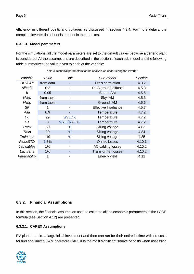
Page 64 Master Thesis
efficiency in different points and voltages as discussed in section 4.9.4. For more details, the
complete inverter datasheet is present in the annexes.
6.3.1.3. Model parameters
For the simulations, all the model parameters are set to the default values because a generic plant
is considered. All the assumptions are described in the section of each sub-model and the following
table summarizes the value given to each of the variable:
Table 3 Technical parameters for the analysis on under-sizing the inverter
Variable Value Unit Sub-model Section
DHI/GHI from data - Erb's correlation 4.3.2
Albedo 0.2 - POA ground diffuse 4.5.3
b 0.05 - Beam IAM 4.5.5
IAMs from table - Sky IAM 4.5.6
IAMg from table - Ground IAM 4.5.6
SF 1 - Effective Irradiance 4.5.7
Alfa 0.9 - Temperature 4.7.2
U0 29 W m2K⁄ Temperature 4.7.2
U1 0 W m2K⁄ m s⁄⁄ Temperature 4.7.2
Tmax 60 Sizing voltage 4.83
Tmin 20 Sizing voltage 4.84
Tmin abs -10 Sizing voltage 4.85
PlossSTD 1.5% - Ohmic losses 4.10.1
Lac cables 1% - AC cabling losses 4.10.2
Lac trans 1% - Transformer losses 4.10.2
Favailability 1 - Energy yield 4.11
6.3.2. Financial Assumptions
In this section, the financial assumption used to estimate all the economic parameters of the LCOE
formula (see Section 4.12) are presented.
6.3.2.1. CAPEX Assumptions
PV plants require a large initial investment and then can run for their entire lifetime with no costs
for fuel and limited O&M, therefore CAPEX is the most significant source of costs when assessing

Development of a model to simulate solar PV plants in MATLAB with a study on the effects of under-sizing the inverter. Page 65
a PV project. Different sources were analyzed to obtain the CAPEX for the PV plant [1], [35], [36].
These sources present different costs, but this is reasonable as the costs are quite dependent on
the region:
Table 4 CAPEX breakdown by different sources
Source [1] [35] [36]
CAPEX modules (eur/kWh) 483 530 375
CAPEX inverter (eur/kWh) 115 110 84
CAPEX BoS (eur/kWh) 552 335 280
CAPEX total 1150 975 739
The data from an European study which provides a cost breakdown for PV plants in Germany [35]
were used because this European study provides a detailed cost breakdown for PV plants in
Germany [35] which is fundamental to understand how much of the cost is related to the AC side
of the plant. The table below shows the cost breakdown:
Figure 22 CAPEX breakdown for large scale PV plants. Source [35].
These data were modified to obtain the cost breakdown divided in the 3 needed sections: Modules,
AC dependent and other costs.
The cost of a plant can be thought of being dependent on:
1. The DC side of the plant, or the number of the solar modules (e.g. solar modules, the
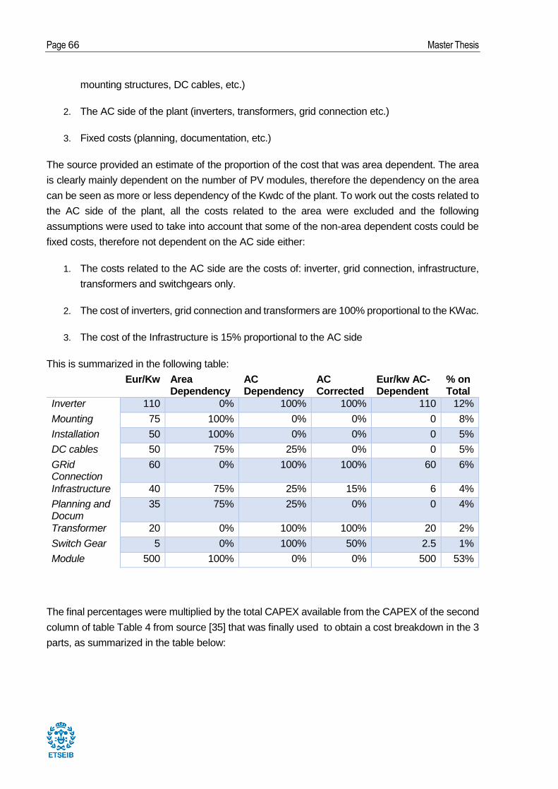
Page 66 Master Thesis
mounting structures, DC cables, etc.)
2. The AC side of the plant (inverters, transformers, grid connection etc.)
3. Fixed costs (planning, documentation, etc.)
The source provided an estimate of the proportion of the cost that was area dependent. The area
is clearly mainly dependent on the number of PV modules, therefore the dependency on the area
can be seen as more or less dependency of the Kwdc of the plant. To work out the costs related to
the AC side of the plant, all the costs related to the area were excluded and the following
assumptions were used to take into account that some of the non-area dependent costs could be
fixed costs, therefore not dependent on the AC side either:
1. The costs related to the AC side are the costs of: inverter, grid connection, infrastructure,
transformers and switchgears only.
2. The cost of inverters, grid connection and transformers are 100% proportional to the KWac.
3. The cost of the Infrastructure is 15% proportional to the AC side
This is summarized in the following table:
Eur/Kw Area Dependency
AC Dependency
AC Corrected
Eur/kw AC-Dependent
% on Total
Inverter 110 0% 100% 100% 110 12%
Mounting 75 100% 0% 0% 0 8%
Installation 50 100% 0% 0% 0 5%
DC cables 50 75% 25% 0% 0 5%
GRid Connection
60 0% 100% 100% 60 6%
Infrastructure 40 75% 25% 15% 6 4%
Planning and Docum
35 75% 25% 0% 0 4%
Transformer 20 0% 100% 100% 20 2%
Switch Gear 5 0% 100% 50% 2.5 1%
Module 500 100% 0% 0% 500 53%
The final percentages were multiplied by the total CAPEX available from the CAPEX of the second
column of table Table 4 from source [35] that was finally used to obtain a cost breakdown in the 3
parts, as summarized in the table below:

Development of a model to simulate solar PV plants in MATLAB with a study on the effects of under-sizing the inverter. Page 67
Table 5 CAPEX breakdown divided by the AC and DC side
Source [35]
CAPEX DC side (eur/kWh) 530
CAPEX AC side (eur/kWh) 255
CAPEX Other (eur/kWh) 335
CAPEX total 975
6.3.2.2. OPEX Assumption
All the sources cited above were consulted to find the value of the OPEX, which was finally taken
as 15 eur/Kw/year from [35] for consistency with the CAPEX assumptions (that were taken from
the same source).
6.3.2.3. WACC Assumptions
As previously said, the WACC have a big impact on the total costs of the plant and on the LCOE.
When WACC increases the cost of capital increases. In other words, it means that for the same
plant, with a higher WACC, a higher part of the revenues goes to investors or as interests thus
increasing the overall cost of the plant. The following graph clearly shows this concept:
Figure 23 LCOE for PV systems as a function of the WACC. Source [37]
As can be seen, higher WACC means higher cost of capital, while all the other costs are constant.

Page 68 Master Thesis
It is remarkable to see that at WACC=10% the cost of capital is roughly 50% of the total cost.
According to the literature, the WACC can be very different in different countries, the following map
shows average WACC values in Europe:
Figure 24 Map of suggested WACC in wind energy projects for different countries in Europe. Source [38]
Even though it is for onshore wind, the source states that for large PV plants in Spain, WACC is
likely to be higher than 10% [30]. Another source mentions values around 7.5 % on a survey done
in Spain [38]. The agency IRENA uses 7.5% for its calculations [1] and another source creates
scenarios from 2% to 10% [5]. Therefore, in the present project values of 7% was used.
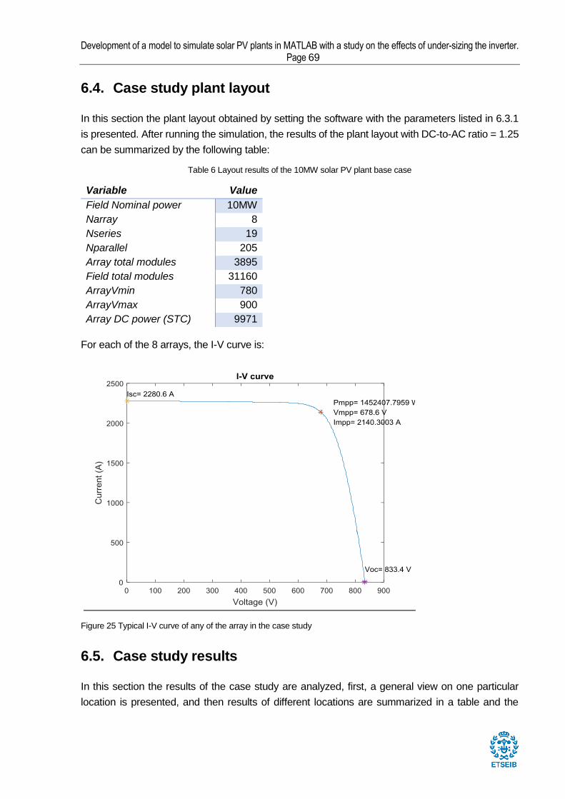
Development of a model to simulate solar PV plants in MATLAB with a study on the effects of under-sizing the inverter. Page 69
6.4. Case study plant layout
In this section the plant layout obtained by setting the software with the parameters listed in 6.3.1
is presented. After running the simulation, the results of the plant layout with DC-to-AC ratio = 1.25
can be summarized by the following table:
Table 6 Layout results of the 10MW solar PV plant base case
Variable Value
Field Nominal power 10MW
Narray 8
Nseries 19
Nparallel 205
Array total modules 3895
Field total modules 31160
ArrayVmin 780
ArrayVmax 900
Array DC power (STC) 9971
For each of the 8 arrays, the I-V curve is:
Figure 25 Typical I-V curve of any of the array in the case study
6.5. Case study results
In this section the results of the case study are analyzed, first, a general view on one particular
location is presented, and then results of different locations are summarized in a table and the

Page 70 Master Thesis
relationship between the DC-to-AC ratio and the mean irradiance is shown.
The graphs below show how LCOE and CF change varying the DC-to-AC ratio for the simulation
performed in Barcelona, and London:
Figure 26 Results of the analysis: LCOE (eur/kwh) and CAPEX versus power ratio in Barcelona, London, Antofagasta and Malaga
The CAPEX of the plant decreases proportionally with the DC-to-AC ratio because the CAPEX of
the AC side of the plant is assumed to be proportional to the installed AC power which decreases
when increasing the DC-to-AC ratio, at a given installed DC power.
The LCOE decreases, reaches a minimum and increases again due to the combined effects of CF
and CAPEX. Before the minimum, for low DC-to-AC ratios, it decreases because the gains in
reduced CAPEX outweigh the slight decrease in CF. The opposite happens after the minimum,
leading to an increase in LCOE. The values of LCOE of around 60eur/kWh for example Barcelona
are compatible with values of Madrid with the same WACC=7% presented in Figure 4 thus meaning
that the parameters of the analysis lead to reasonable results.
If the capacity factor is analyzed, for example for London, which is quite an extreme case as it is
affected by low mean irradiance, the results would be as follows:
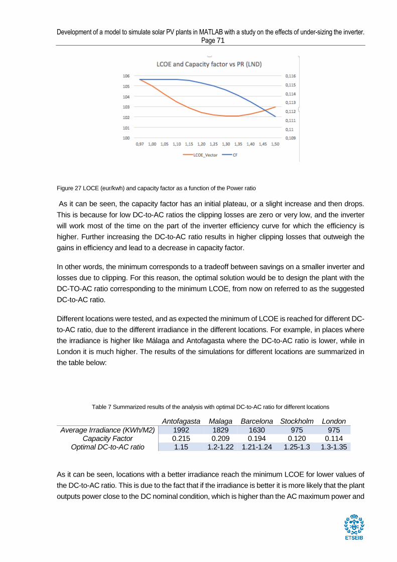
Development of a model to simulate solar PV plants in MATLAB with a study on the effects of under-sizing the inverter. Page 71
Figure 27 LOCE (eur/kwh) and capacity factor as a function of the Power ratio
As it can be seen, the capacity factor has an initial plateau, or a slight increase and then drops.
This is because for low DC-to-AC ratios the clipping losses are zero or very low, and the inverter
will work most of the time on the part of the inverter efficiency curve for which the efficiency is
higher. Further increasing the DC-to-AC ratio results in higher clipping losses that outweigh the
gains in efficiency and lead to a decrease in capacity factor.
In other words, the minimum corresponds to a tradeoff between savings on a smaller inverter and
losses due to clipping. For this reason, the optimal solution would be to design the plant with the
DC-TO-AC ratio corresponding to the minimum LCOE, from now on referred to as the suggested
DC-to-AC ratio.
Different locations were tested, and as expected the minimum of LCOE is reached for different DC-
to-AC ratio, due to the different irradiance in the different locations. For example, in places where
the irradiance is higher like Málaga and Antofagasta where the DC-to-AC ratio is lower, while in
London it is much higher. The results of the simulations for different locations are summarized in
the table below:
Table 7 Summarized results of the analysis with optimal DC-to-AC ratio for different locations
Antofagasta Malaga Barcelona Stockholm London
Average Irradiance (KWh/M2) 1992 1829 1630 975 975 Capacity Factor 0.215 0.209 0.194 0.120 0.114
Optimal DC-to-AC ratio 1.15 1.2-1.22 1.21-1.24 1.25-1.3 1.3-1.35
As it can be seen, locations with a better irradiance reach the minimum LCOE for lower values of
the DC-to-AC ratio. This is due to the fact that if the irradiance is better it is more likely that the plant
outputs power close to the DC nominal condition, which is higher than the AC maximum power and
Page 72 Master Thesis
therefore the excess power is clipped. etc.
It is interesting the case of London and Stockholm have the same average yearly irradiance, while
different capacity factor. The reason behind it is that in London the lower frequency at which STD
conditions are reached means that most of the time the system will output DC power much lower
than the nominal DC power, and this is the reason why a higher DC-to-AC ratio is suggested. On
the other hand, in Stockholm the frequency of STD conditions is higher, and the system is more
likely to output DC power closer to the DC nominal power, thus increasing the clipping losses if the
inverter is too small, therefore a lower DC-to-AC ratio is suggested.
6.6. Case study conclusions
The case study proved that it makes financial sense to oversize the solar field with respect to the
inverter. The values of LCOE of around 60eur/kWh for example Barcelona are compatible with
values of Madrid with the same WACC=7% presented in Figure 4 thus meaning that the parameters
of the analysis lead to reasonable results. Reduction in the investment of the inverter is around 15-
35%, which in turns decreases the total CAPEX by 3-5%. The reduction in total capex is of course
lower as the AC side of the plant accounts for roundabout 20% of the investment. Reduction in
LCOE due to optimal Dc-to-AC ratio ranges between 3.3%-3.7% depending on the location.
It should be noted that the case study did not take into account the possible consequences of
under-sizing the inverter on the reliability and maintenance costs of the inverter itself. This is linked
to the behavior of the components inside the inverter, which is another interesting study case
studied for example in [32] but out of the scope of this project. As a future work, it would be
interesting to combine both aspects together to obtain a more comprehensive result.

Development of a model to simulate solar PV plants in MATLAB with a study on the effects of under-sizing the inverter. Page 73
7. Planning, costs and environmental impact of this
project
7.1. Environmental Impact of the project
D
As with the economics, the environmental impact of a solar PV plant will be calculated for the 10MW
plant described in section 6.4. The environmental impact due to greenhouse gases (GHG)
emissions is treated in the following sections.
7.1.1. Emissions of a solar PV plant with life cycle assessment
To calculate the environmental impact of an electricity generation technology, it is usual practice to
consider the life cycle assessment (LCA). The LCA takes into account all the emissions of a
technology, dividing the lifecycle of a plant in three phases: upstream process (manufacturing, plant
construction etc.), operational process (power generation, fuel needed, O&M, etc.) and
downstream process (power plant decommissioning, disposal etc.) as shown by the figure below:
Figure 28 The three stages of the lifecycle of PV and Coal plant. Source NREL [39].
Calculating a LCA in details is a complex topic that alone require another study and is often
subjected to discrepancies. Therefore, for the analysis of this section, the data obtained from a
study by NREL will be used [39]. The analysts reviewed more than 400 studies and considering a
lifetime of 30 years, they finally conclude that the LCA greenhouse gases emissions of crystalline
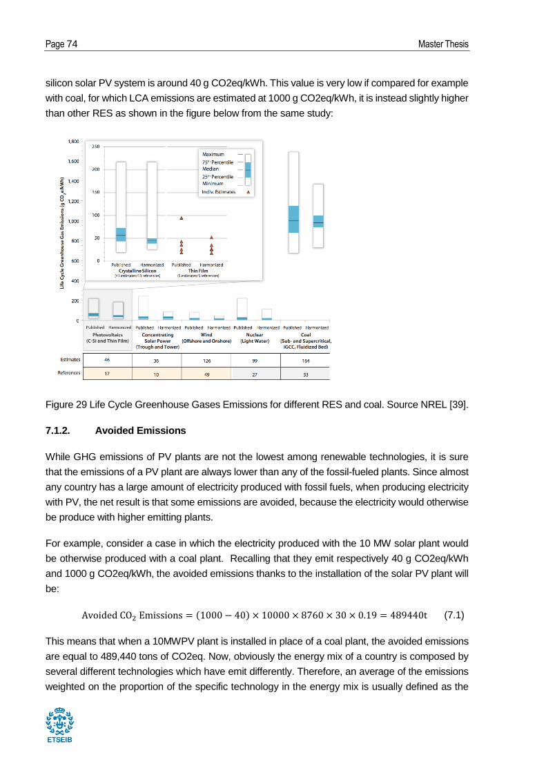
Page 74 Master Thesis
silicon solar PV system is around 40 g CO2eq/kWh. This value is very low if compared for example
with coal, for which LCA emissions are estimated at 1000 g CO2eq/kWh, it is instead slightly higher
than other RES as shown in the figure below from the same study:
Figure 29 Life Cycle Greenhouse Gases Emissions for different RES and coal. Source NREL [39].
7.1.2. Avoided Emissions
While GHG emissions of PV plants are not the lowest among renewable technologies, it is sure
that the emissions of a PV plant are always lower than any of the fossil-fueled plants. Since almost
any country has a large amount of electricity produced with fossil fuels, when producing electricity
with PV, the net result is that some emissions are avoided, because the electricity would otherwise
be produce with higher emitting plants.
For example, consider a case in which the electricity produced with the 10 MW solar plant would
be otherwise produced with a coal plant. Recalling that they emit respectively 40 g CO2eq/kWh
and 1000 g CO2eq/kWh, the avoided emissions thanks to the installation of the solar PV plant will
be:
Avoided CO2 Emissions = (1000 − 40) × 10000 × 8760 × 30 × 0.19 = 489440t (7.1)
This means that when a 10MWPV plant is installed in place of a coal plant, the avoided emissions
are equal to 489,440 tons of CO2eq. Now, obviously the energy mix of a country is composed by
several different technologies which have emit differently. Therefore, an average of the emissions
weighted on the proportion of the specific technology in the energy mix is usually defined as the

Development of a model to simulate solar PV plants in MATLAB with a study on the effects of under-sizing the inverter. Page 75
grid emission factor. Taking the case of Spain, the grid emission factor was considered to be 343
g CO2eq/kWh in 2013, calculated with the LCA method in a study by the European Union [40]. In
this case, the avoided emissions thanks to the installation of the 10MW solar PV plants will be:
Avoided CO2 Emissions = (343 − 40) × 10000 × 8760 × 30 × 0.19 = 151290t (7.2)
Still, installing a 10MWPV plant in same would save the emissions of 151,290 tons of CO2eq. This
reasoning could be repeated for any other country and there will be always some avoided
emissions, unless the country has an emission factor lower than 40 g CO2eq/kWh, which is not the
case in any of the European countries [40]. Therefore, installing solar PV panels, is always a
solution that reduces the GHG emissions, even considering the manufacturing and the disposal of
the panels.

Page 76 Master Thesis
8. Conclusions
Results of the program against results from PVsyst showed that the hourly RMSE for the DC power
is 0.26%, leading to the conclusion that the program developed in the present project simulates
well the parameters of a PV plant and it is a good starting point for a possible further development.
The case study proved that it makes financial sense to oversize the solar field with respect to the
inverter. The values of LCOE of around 60eur/kWh for example Barcelona are compatible with
values of Madrid with the same WACC=7% presented in Figure 4 thus meaning that the parameters
of the analysis lead to reasonable results. Reduction in the investment of the inverter is around 15-
35%, which in turns decreases the total CAPEX by 3-5%. The reduction in total capex is of course
lower as the AC side of the plant accounts for roundabout 20% of the investment. Reduction in
LCOE due to optimal Dc-to-AC ratio ranges between 3.3%-3.7% depending on the location.
This project was developed from zero, therefore the scope has to be limited to the models described
in Section4.2. Nevertheless, it was precisely the of the project to develop a software that could be
further developed by other students or researchers. During the developing of the software,
interesting topics were encountered that could be further studied, as an example:
1. A detailed model of the control scheme of the plant or integrating this model to other models
to analyze different issues related to PV (such as the integration to the grid etc.)
2. A model to retrieve the model parameters of the I-V curve of the single diode model from
experimental measurements done at different T and G.
3. A model to consider the self-shading losses due to adjacent rows.
4. A study on the techno-economic strategy to design the optimum number of inverters given
a plant size.
5. A study that considers the effects of under-sizing the inverter on the reliability of the inverter
itself
This is a list of possible problems that were encountered and could not be analyzed due to time
restrictions, but could certainly be extended by others.
Development of a model to simulate solar PV plants in MATLAB with a study on the effects of under-sizing the inverter. Page 77
Bibliography
[1] IRENA, “Renewable Power Generation Costs in 2017,” 2018.
[2] IEA, “Photovoltaic Power Systems Programme - PVPS Annual Report 2016,” Int. Energy Agency, p. 130, 2016.
[3] European Commision Energy Roadmap 2050, “Communication from the Commission to the European Parliament, the Council, the European Economic and Social Committee and the Committee of the Regions, COM/2011/0885 final.,” 2011.
[4] P. Altermatt, Photovoltaic Solar Energy: From Fundamentals to Applications. 2017.
[5] E. Vartiainen et al., “The True Competitiveness of Solar PV - A European Case Study,” 2017.
[6] J. A. Duffie and W. A. Bekman, Solar Engineering of Thermal Processes. Wiley, 2013.
[7] K. J. Sauer and T. Roessler, “Systematic approaches to ensure correct representation of measured multi-irradiance module performance in PV system energy production forecasting software programs,” IEEE J. Photovoltaics, vol. 3, no. 1, pp. 422–428, 2013.
[8] A. Mermoud, “PVsyst 6 Help,” PVsyst SA, 2018. [Online]. Available: http://files.pvsyst.com/help/. [Accessed: 01-Apr-2018].
[9] P. Gilman, A. Dobos, N. DiOrio, J. Freeman, S. Janzou, and D. Ryberg, “SAM Photovoltaic Model Technical Reference SAM Photovoltaic Model Technical Reference,” 2018.
[10] B. Y. H. Liu and R. C. Jordan, “The interrelationship and characteristic distribution of direct, diffuse and total solar radiation,” Sol. Energy, vol. 4, no. 3, pp. 1–19, Jul. 1960.
[11] R. R. Perez, P. Ineichen, E. L. Maxwell, R. D. Seals, and A. Zelenka, “Dynamic global-to-direct irradiance conversion models,” in ASHRAE Transactions, 1992.
[12] College of Engineering and Applied Science University of Colorado Boulder, “Solar Angles and Tracking Systems - Lesson - TeachEngineering,” Integrated Teaching and Learning Program. [Online]. Available: https://www.teachengineering.org/lessons/view/cub_pveff_lesson01. [Accessed: 20-Jul-2018].
[13] Seaward Group USA, “Frequently asked questions about Curve Tracing.” [Online]. Available: http://www.seaward-groupusa.com/userfiles/curve-tracing.php. [Accessed: 20-Jul-2018].
[14] T. Maor and J. Appelbaum, “View factors of photovoltaic collector systems,” Sol. Energy, vol. 86, no. 6, pp. 1701–1708, 2012.
[15] PVsyst SA, “PVsyst Photovoltaic Software 6.7.3.” 2018.
[16] N. Pearsall, The performance of photovoltaic (PV) systems : modelling, measurement and assessment. Woodhead Publishing, 2017.
[17] K. J. Sauer, T. Roessler, and C. W. Hansen, “Modeling the irradiance and temperature dependence of photovoltaic modules in PVsyst,” IEEE J. Photovoltaics, vol. 5, no. 1, pp.

Page 78 Master Thesis
152–158, 2015.
[18] A. Mermoud and T. Lejeune, “Performance Assessment of a Simulation Model for Pv Modules of Any Available Technology,” 25th Eur. PV Sol. Energy Conf., no. September, pp. 6–10, 2010.
[19] A. Quarteroni and F. Saleri, Calcolo scientifico: Esercizi e problemi risolti con MATLAB e Octave. 2008.
[20] D. Faiman, “Assessing the outdoor operating temperature of photovoltaic modules,” Prog. Photovoltaics Res. Appl., vol. 16, no. 4, pp. 307–315, 2008.
[21] UPC, “Photovoltaic Solar Energy- Course at UPC.” 2017.
[22] ABB, “ABB central inverters PVS800 100 to 500 kW - Datasheet,” p. 6, 2013.
[23] KTH, “Renewable Energy Technology 2 - Course at KTH.” 2016.
[24] ABB, “ABB central inverter, PVS800, now available up to 2 MW size,” 2017. [Online]. Available: http://www.abb.com/cawp/seitp202/c7e6d5056e761ac5c1258163003d3612.aspx. [Accessed: 20-Jul-2018].
[25] D. L. King, S. Gonzalez, G. M. Galbraith, and W. E. Boyson, “Performance Model for Grid-Connected Photovoltaic Inverters,” Albuquerque, New Mexico 87185 and Livermore, California 94550, 2007.
[26] A. Driesse, P. Jain, and S. Harrison, “Beyond the curves: Modeling the electrical efficiency of photovoltaic inverters,” in Conference Record of the IEEE Photovoltaic Specialists Conference, 2008.
[27] IRENA, “RESOURCE Your Source for Renewable Energy - Data Methodology,” 2015. [Online]. Available: http://dashboard.irena.org/download/Methodology.pdf. [Accessed: 01-Jul-2018].
[28] C. Tjengdrawira, M. Richter, and I. T. Theologitis, “Best Practice Guidelines for PV Cost Calculation,” 2016.
[29] LAZARD, “Lazard’s Levelized Cost of Energy Analysis - Version 11.0,” 2017.
[30] P. Noothout, D. de Jager, and et al., “The impact of risks in renewable energy investments and the role of smart policies,” 2016.
[31] K. Zipp, “Why array oversizing makes financial sense,” Solar Power World, p. 5, 2018.
[32] A. Sangwongwanich, Y. Yang, D. Sera, F. Blaabjerg, and D. Zhou, “On the Impacts of PV Array Sizing on the Inverter Reliability and Lifetime,” IEEE Trans. Ind. Appl., vol. 54, no. 4, pp. 3656–3667, 2018.
[33] Jinko Solar, “Jinko Solar | Your Best Supplier of Modules,Cells & Wafers,” 2018. [Online]. Available: https://www.jinkosolar.com/about_207.html. [Accessed: 20-Jul-2018].
[34] T. Toissalo, “Aurinkoinverttereitä maailmalle-Aurinkoinen pientuotanto -ABB seminaari,” 2017.

Development of a model to simulate solar PV plants in MATLAB with a study on the effects of under-sizing the inverter. Page 79
[35] E. Vartiainen, G. Masson, and C. Breyer, “PV LCOE In Europe 2014-30 - Final Report,” 2015.
[36] Spain’s Photovoltaic Union - UNEF and International Energy Agency - IEA, “National Survey Report of PV Power Applications in Spain,” 2015.
[37] A. Jäger-waldau, PV Status Report 2016, no. October. 2016.
[38] Grant Thornton, “Renewable energy discount rate survey results – 2017,” 2018.
[39] NREL, “Life Cycle Greenhouse Gas Emissions from Solar Photovoltaics,” p. 2, 2012.
[40] B. Koffi, A. Cerutti, M. Duerr, A. Iancu, A. Kona, and G. Janssens-Maenhout, “CoM Default Emission Factors for the Member States of the European Union Dataset -Version 2017, European Commission, Joint Research Centre (JRC),” 2017.