development of a model to be used as an indicator of …
TRANSCRIPT

DEVELOPMENT OF A MODEL TO BE USED AS AN INDICATOR OF OILY
WASTEWATER POLLUTION, FINGERPRINTING AND COMPLIANCE USING
DIMENSIONAL ANALYSIS
by
Lerato Elizabeth Monatisa
Dissertation submitted in fulfilment of the requirements for the degree of
MAGISTER TECHNOLOGIAE
in
CHEMICAL ENGINEERING
in the
COLLEGE OF SCIENCE, ENGINEERING AND TECHNOLOGY
of the
UNIVERSITY OF SOUTH AFRICA
Supervisor: PROF TITUS A.M MSAGATI
Co-supervisors: PROF THABO T.I NKAMBULE
PROF BHEKIE B MAMBA
Dr. AZIZALLAH IZADY
Dr. LUETA de KOCK
September 2020

i
DECLARATION
Name: Lerato Monatisa
Student number: 62697765
Degree: Magister Technologiae: Chemical Engineering
DEVELOPMENT OF A MODEL TO BE USED AS AN INDICATOR OF OILY
WASTEWATER POLLUTION, FINGERPRINTING AND COMPLIANCE USING
DIMENSIONAL ANALYSIS
I, with this dissertation declare that it is my own work and that all the quoted and used sources
have been shown and recognised by means of complete references.
SIGNATURE ________________________ DATE _____________________

ii
DEDICATION
This dissertation is dedicated to my two beautiful daughters, Kutloano Monatisa and Bonang
Monatisa, a special thanks to you my angels for being my source of inspiration and always
encouraging mommy to always do her best. My life is incomplete without you.
My younger brother Thabang Monatisa for always being there for me whenever I need you, I
will always love you.
In loving memory of my late parents Keneuwe Margaret Monatisa and Daniel Boy Maleke. I am
the strongest woman today because of your love and guidance. I know you watching down on
me, you will always be in my heart.
"I Can Do All Things Through Christ Who Strengthens Me" (Philippians 4:13)

iii
PRESENTATIONS AND PUBLICATIONS
Presentations:
Lerato E. Monatisa, Azizallah Izady, Lueta de Kock, Bhekie B. Mamba and Nkambule T.I and
Titus A.M. Msagati (2019). Development of a model to be used as an indicator of oily
wastewater pollution, fingerprinting and compliance using dimensional analysis. Oral
Presentation. US- Africa Forum. Nanotechnology Convergence for Sustainable Energy, Water
and Environment. Glenburn Lodge & Spa. Kromdaai Road. Mudeldrift. Johannesburg. South
Africa. 11st - 15th August 2019.
Lerato E. Monatisa, Azizallah Izady, Lueta de Kock, Bhekie B. Mamba and Nkambule TI and
Titus A.M. Msagati (2019). Development of a model to be used as an indicator of oily
wastewater pollution, fingerprinting and compliance using dimensional analysis. Poster
presentation. 2nd International Symposium on Environment and Energy Science & Technology
ISEEST-2. Misty Hills. Johannesburg. South Africa. 18th -21st August 2019.
Peer-Reviewed Journal Articles Publications:
Manuscripts under preparation
1. Identification of Total Petroleum Hydrocarbons (TPH) in Oil Produced Water (OPW)
Samples.
2. Influence of environmental and climatic factors on the evaporation rate of wastewater.
3. Use of Dimensional Analysis to develop a model to predict quality and compliance of
oily wastewater discharged onto municipal channels.

iv
ACKNOWLEDGEMENTS
I would like to give thanks to the heavenly Father, Son and the Holy Spirit for giving me
strength, patience and perseverance to complete this research. If it were not for your love and
your guidance I wouldn’t have made this far.
This work was only possible with people and organizations for support, contributions, and
encouragement towards my project. I would like to acknowledge the following individuals and
organizations:
▪ My supervisor, Prof Titus Msagati for granting me this lifetime opportunity to work
under your team of supervision. Thank you for believing in me that I could handle this
project, even I was pregnant you saw the potential in me. You have taught me to always
have a bigger picture even though things were tough, thank you for everything.
▪ To my co-supervisors, Prof Thabo Nkambule, Dr Azizallah Izady, Prof Bhekie Mamba
and Dr Lueta de Kock thank you so much for the moral support throughout this journey.
Your time and effort to guide me through my project is much appreciated.
▪ Dr Hlengilizwe Nyoni and Mr Kagiso Mokalane for giving me access to the laboratories
and for giving me instrumental trainings so can I meet the objectives of my studies. I
have learned a lot from you, thank you.
▪ Chemical Engineering department for giving me access to the GC-MS, Mr Osley
Mathebula thank you for giving me the GC-MS training, humbly appreciated for your
time and effort out of your busy schedule.
▪ Department of Chemistry for allowing me to use the turbo-vac instrument.
▪ Mr Amoudjata Sacko for stepping in and assisting me to understand GC-MS better
(theoretical and technical information). I learned a lot from you and you really came
through for me whenever I needed you, thanks a lot.
▪ Mr Terrence Malatjie for always assisting me with the presentation’s skills. Through you
I learned to give the best presentations.
▪ Miss Ellen Kwenda for assisting me with the spectroquant spectrophotometer.
▪ University of South Africa (UNISA) through the Institute of Nanotechnology Water
Sustainability (iNanoWS) and National Research Foundation (NRF) for providing
bursary.

v
▪ Water Research Centre (WRC) from Sultan Qaboos University (SQU) in Oman for a
warm welcome when I came there for my training. I really enjoyed my stay.
▪ Miss Precious Sithole and Miss Ratanang Mlaba for moral support throughout my
journey.
▪ My family for their undying support especially my daughters, Kutloano Monatisa and
Bonang Monatisa for understanding when I was not able to spend quality time with them
more often because I had to be in the laboratory most of the time. I am glad they are
happy that it was worth it. My brother Thabang Monatisa, your love and support give me
hope to always fight to be the best in life. My partner, Tshepo Molebaloa for believing
and encouraging me to pursue my studies even though I was pregnant with our second
child. Last but not the least, my spiritual parents who God has blessed me with, Mr &
Mrs Lekgau. Your love and guidance are much appreciated, I will always love you.

vi
ABSTRACT
Water is the source of life because all living organisms cannot survive without it and it is the
most important liquid in the ecosystem hence protecting water resources and ensuring water
quality should always be an issue of the highest priority at the top of all environmental issues.
Currently, both developing and developed countries are experiencing numerous water quality
challenges. Among the challenges include lack of adequate water due to pollution as well as the
management and disposal of oily wastewater effluents in water resources. Regarding the issue of
pollution due to oily wastewater, the current trend shows that, with the increase in
industrialization, the amount of oil used is also increasing, thus causing more stress in terms of
management and treatment of wastewater. Oily wastewater pollution has mainly been reported to
cause hazardous effects to both organisms and the environment by causing the deterioration of
aquatic resources. This in-turn affect the quality of ground water, surface water, endanger human
health, cause of atmospheric pollution, destroy/degrade natural landscape, and even cause safety
issues due to the use of coalescence of the oil burner that arise. Due to this phenomena, various
regulatory bodies have established some guidelines to regulate the disposal of oily wastewater
that is discharged to the environment. Therefore, oily wastewater needs to be treated prior to
being discharged into the environment to comply with state and local disposal regulations.
Industries and companies that deal with activities that lead to the discharge of oily wastewater
need to comply to the enforced regulations to ensure that the characteristic of their effluents meet
the stipulated disposal criteria. The effluent quality requirements for discharge of oily
wastewater to the municipal streams are determined by local and municipal authorities and, they
may vary from place to place. This dissertation focused on the development of a model that can
be used to indicate the quality of oily wastewater known as oil -produced water (OPW) which is
normally discharged by petroleum industries to into receiving water bodies. The model
development was accomplished by using a measure of evaporation patterns in relation to certain
environmental and climatic variables. This is possible because certain physico-chemical
parameters that normally characterize OPW are known to have a direct relationship with the rate
and pattern of OPW evaporation. However, due to the complexity of the relationship between the
parameters being measured, it was imperative to employ dimensional analysis approach that is
based on Buckingham pi () theorem for the estimation of oil produced water evaporation
vii
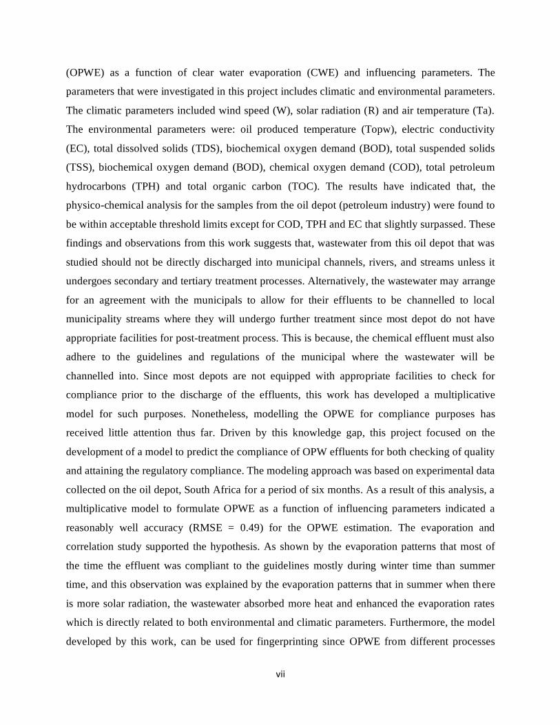
(OPWE) as a function of clear water evaporation (CWE) and influencing parameters. The
parameters that were investigated in this project includes climatic and environmental parameters.
The climatic parameters included wind speed (W), solar radiation (R) and air temperature (Ta).
The environmental parameters were: oil produced temperature (Topw), electric conductivity
(EC), total dissolved solids (TDS), biochemical oxygen demand (BOD), total suspended solids
(TSS), biochemical oxygen demand (BOD), chemical oxygen demand (COD), total petroleum
hydrocarbons (TPH) and total organic carbon (TOC). The results have indicated that, the
physico-chemical analysis for the samples from the oil depot (petroleum industry) were found to
be within acceptable threshold limits except for COD, TPH and EC that slightly surpassed. These
findings and observations from this work suggests that, wastewater from this oil depot that was
studied should not be directly discharged into municipal channels, rivers, and streams unless it
undergoes secondary and tertiary treatment processes. Alternatively, the wastewater may arrange
for an agreement with the municipals to allow for their effluents to be channelled to local
municipality streams where they will undergo further treatment since most depot do not have
appropriate facilities for post-treatment process. This is because, the chemical effluent must also
adhere to the guidelines and regulations of the municipal where the wastewater will be
channelled into. Since most depots are not equipped with appropriate facilities to check for
compliance prior to the discharge of the effluents, this work has developed a multiplicative
model for such purposes. Nonetheless, modelling the OPWE for compliance purposes has
received little attention thus far. Driven by this knowledge gap, this project focused on the
development of a model to predict the compliance of OPW effluents for both checking of quality
and attaining the regulatory compliance. The modeling approach was based on experimental data
collected on the oil depot, South Africa for a period of six months. As a result of this analysis, a
multiplicative model to formulate OPWE as a function of influencing parameters indicated a
reasonably well accuracy (RMSE = 0.49) for the OPWE estimation. The evaporation and
correlation study supported the hypothesis. As shown by the evaporation patterns that most of
the time the effluent was compliant to the guidelines mostly during winter time than summer
time, and this observation was explained by the evaporation patterns that in summer when there
is more solar radiation, the wastewater absorbed more heat and enhanced the evaporation rates
which is directly related to both environmental and climatic parameters. Furthermore, the model
developed by this work, can be used for fingerprinting since OPWE from different processes

viii
may have similar chemical composition but in different levels and ratios. This can be exploited
to differentiate them using the same developed model as the coefficients pattern tend to be
characteristic to a certain OPWE and the model can then be used to fingerprint and identify
culprits in case of discrepancies.

ix
TABLE OF CONTENT
DECLARATION ................................................................................................................................. i
DEDICATION ....................................................................................................................................ii
PRESENTATIONS AND PUBLICATIONS................................................................................ iii
ACKNOWLEDGEMENTS ............................................................................................................. iv
ABSTRACT ........................................................................................................................................ vi
TABLE OF CONTENT .................................................................................................................... ix
LIST OF FIGURES AND SCHEMES .......................................................................................... xv
LIST OF TABLES ...........................................................................................................................xvi
LIST OF ABBREVIATIONS ..................................................................................................... xviii
CHAPTER 1 : INTRODUCTION ....................................................................................................... 1
1.1 Background.................................................................................................................................... 1
1.2 Problem Statement ........................................................................................................................ 4
1.3 Justification ................................................................................................................................... 5
1.4 Aims and Objectives....................................................................................................................... 6
1.4.1 Aims ........................................................................................................................................ 6
1.4.2 Objectives ............................................................................................................................... 6
1.5 Dissertation outline ....................................................................................................................... 7
1.6 References ..................................................................................................................................... 8
CHAPTER 2 : LITERATURE REVIEW ......................................................................................... 11
2.1 Environmental concerns of discharge of oily wastewater ............................................................. 11
2.2 The impact of pollution from the oil depot ................................................................................... 12
2.3 Oil produced water from oil production ....................................................................................... 12
2.4 Regulations of the discharge of produced water. ......................................................................... 13
2.5 Environmental effect of petroleum pollution to the environment ................................................ 14
2.6 Characteristics of oil Produced Water .......................................................................................... 16
Quantitative assessments of the quality of the OPW are made by considering the following
parameters: ....................................................................................................................................... 16

x
2.6.1 Water Temperature .............................................................................................................. 16
2.6.2 Total suspended solids (TSS).................................................................................................. 16
2.6.3 Total dissolved solids (TDS) ................................................................................................... 17
2.6.4 Electrical conductivity (EC) .................................................................................................... 17
2.6.5 Biochemical oxygen demand (BOD) ....................................................................................... 17
2.6.6 Chemical oxygen demand (COD) ........................................................................................... 18
2.6.7 Total organic carbon (TOC) .................................................................................................... 18
2.6.8 Quantification methods for organic matters .......................................................................... 19
2.6.9 Total petroleum hydrocarbons (TPH)..................................................................................... 19
2.7 Analytical methods for the determination of TPH in water ........................................................... 20
2.7.1 Sample pre-treatment methods for TPH ................................................................................ 21
2.7.2 Separation and detection methods for TPH ........................................................................... 22
2.8 Gas Chromatography-Mass Spectrometry .................................................................................... 22
2.9 Evaporation principles ................................................................................................................. 22
2.9.1 Water quality ........................................................................................................................ 24
2.9.2 Water depth.......................................................................................................................... 24
2.9.3 Water Vapour ....................................................................................................................... 24
2.9.4 Rainfall .................................................................................................................................. 24
2.10 Meteorological factors affecting the rate of evaporation ........................................................... 25
2.10.1 Air Temperature .................................................................................................................. 25
2.10.2 Water temperature ............................................................................................................. 25
2.10.3 Solar radiation ..................................................................................................................... 25
2.10.4 Wind speed ......................................................................................................................... 25
2.11 Methods used for estimation of open evaporation..................................................................... 26
2.11.1 Mass or bulk transfer balance ............................................................................................. 26
2.11.2 Energy balance method ....................................................................................................... 26
2.11.3 Bulk or mass transfer........................................................................................................... 27
2.11.4 Combination equations ....................................................................................................... 28
2.11.5 The equilibrium temperature method ................................................................................. 28
2.11.6 A pan measurement ............................................................................................................ 28
2.12 Application of the estimation of evaporation of open surface using different models. ............... 29
2.13 Development of a mathematical model ..................................................................................... 31

xi
2.14 Buckingham theorem .............................................................................................................. 32
2.15 Conclusion ................................................................................................................................. 33
2.16 References ................................................................................................................................. 34
CHAPTER 3 : RESEARCH METHODOLOGY ............................................................................. 45
3.1 Materials and methods ................................................................................................................ 45
3.1.1 Chemicals and materials........................................................................................................ 45
3.1.2 Apparatus ............................................................................................................................. 45
3.1.3 Instrumentation .................................................................................................................... 45
3.2 Class A evaporation pan and field deployment ............................................................................. 46
3.2.1 Fabrication of Class A pan...................................................................................................... 46
3.3 Field Measurements .................................................................................................................... 47
3.3.1 Evapoartion rate measurements principle ............................................................................. 47
3.3.2 Measurements of environmental parameters in the field ...................................................... 48
3.3.3 Measurements of climatic parameters .................................................................................. 48
3.4 Description of oil depot works ..................................................................................................... 49
3.5 Laboratory measurements ........................................................................................................... 50
3.5.1 Sample collection and sample pre-treatment ........................................................................ 50
3.6 Spectroquant spectrophotometer instrumentation...................................................................... 50
3.6.1 BOD colorimetric method...................................................................................................... 50
3.6.1.2 Measurements of BOD ....................................................................................................... 51
3.6.2 Measurements of COD .......................................................................................................... 52
3.6.2.2 COD measurements by a colometric method...................................................................... 52
3.6.3 TOC measurements ............................................................................................................... 55
3.6.3.1 Measurements of TOC ........................................................................................................ 55
3.6.4 Total suspended solids (TSS).................................................................................................. 55
3.6.4.1 Measurements of total suspended solids (TSS) ................................................................... 55
3.7 Total petroleum hydrocarbons (TPH) ........................................................................................... 57
3.7.1 Sample preparation for extraction of petroleum compounds in oil-produced water .............. 57
3.7.2 Clean-up of LLE extracts using silica gel ................................................................................. 60
3.7.3 Preparation of standard solutions for GC x GC-TOF MS .......................................................... 62
3.7.4 Measurements of TPH using GC x GC-TOF-MS ....................................................................... 62

xii
3.8 Model development .................................................................................................................... 62
3.8.1 Establishing units of measurements in the model development ............................................ 62
3.9 OPWE Equation Derivation .......................................................................................................... 64
3.10 Statistical analysis ...................................................................................................................... 66
3.11 Compliance study ...................................................................................................................... 66
3.12 References ................................................................................................................................. 67
CHAPTER 4 : IDENTIFICATION OF TOTAL PETROLEUM HYDROCARBONS IN OIL
PRODUCED WATER ....................................................................................................................... 68
4.1 Introduction................................................................................................................................. 68
4.2 The development and optimization of the separation and detection method for TPHs using GC-
TOF-MS ............................................................................................................................................. 69
4.3 Liquid – Liquid Extraction (LLE) of TPHs from OPW ....................................................................... 71
4.3.1 Effect of the organic phase on the extraction efficiency......................................................... 72
4.3.2 Optimization of organic solvent and the determination of extraction recovery efficiency ...... 72
4.4 Calibration experiments ............................................................................................................... 73
4.5 Limit of detection and quantification determination using GC-MS................................................ 74
4.6 Quality Control ............................................................................................................................ 75
4.7 Analysis of TPHs in samples collected from petroleum industry. .................................................. 75
4.7.1 Measurements of TPHs in oil produced water ....................................................................... 75
4.7.2 GC-MS analysis of blank samples ........................................................................................... 75
4.7.3 Alkane hydrocarbons in the influent samples in autumn 2019 ............................................... 77
4.8 Winter profile of TPHs in oil produced water samples from an oil petroleum industry ................. 83
4.8.1 TPH Profile in Spring and Summer. ........................................................................................ 95
4.9 Conclusion ................................................................................................................................... 95
4.10 References ................................................................................................................................. 96
CHAPTER 5 : INVESTIGATION OF PHYSICO-CHEMICAL PARAMETERS OF OIL
PRODUCED WATER DISCHARGE EFFLUENT FROM A PETROLEUM INDUSTRY........ 98
5.1 Introduction................................................................................................................................. 98
5.1.1 Physico-chemical parameters from petroleum industry effluents. ......................................... 98
5.1.2 Characteristics of petroleum wastewater .............................................................................. 99
5.2 Assessment of Physicochemical Parameters in a Selected Oil Depot: ........................................... 99
5.2.1 Total Dissolved Solids (TDS) ................................................................................................. 100

xiii
5.2.2 Electrical conductivity (EC) .................................................................................................. 101
5.2.3 Measurements of Biochemical oxygen demand (BOD) ........................................................ 109
5.2.4 Chemical Oxygen Demand (COD)......................................................................................... 110
5.2.5 Total organic carbon (TOC) .................................................................................................. 111
5.2.6 Total suspended solids (TSS)................................................................................................ 111
5.2.7 Total petroleum hydrocarbons (TPH)................................................................................... 112
5.3 Prediction of compliance of oil produced water using the evaporation rate patterns. ................ 113
5.3.1 Estimation of oil produced evaporation ............................................................................... 113
5.3.2 Clear water evaporation (CWE) v/s oil produced water evaporation (OPWE) ....................... 114
5.3.3 Effect of the climatic parameters on the rate of evaporation ............................................... 116
5.3.4 Air temperature (Ta) ............................................................................................................ 116
5.3.5 Solar radiation..................................................................................................................... 119
5.3.6 Wind speed ......................................................................................................................... 121
5.3.7 Water temperature (Tw) ..................................................................................................... 123
5.4 Effect of the climatic parameters on the rate of evaporation ..................................................... 124
5.4.1 Total dissolved solids (TDS) ................................................................................................. 124
5.4.2 Electrical conductivity (EC) .................................................................................................. 126
5.4.3 Organic carbons (BOD, COD, and TOC) ................................................................................ 127
5.4.4 Total suspended solids (TSS)................................................................................................ 128
5.4.5 Total petroleum hydrocarbons (TPH)................................................................................... 129
5.4.6 Comparison with literature data .......................................................................................... 131
5.5 The correlation studies .............................................................................................................. 133
5.6 Conclusion ................................................................................................................................. 136
5.7 References ................................................................................................................................. 137
CHAPTER 6 : DEVELOPMENT OF THE OIL PRODUCED WATER MODEL TO BE USED
FOR ASCERTAINING THE COMPLIANCE TO GUIDELINES .............................................. 142
6.1 Introduction............................................................................................................................... 142
6.2 Model development based on Buckingham pi theorem. ............................................................ 143
6.2.1 Obtaining the coefficients ................................................................................................... 143
6.2.2 Statistical analysis ............................................................................................................... 144
6.2.3 Estimation of OPWE using dimensional analysis results ....................................................... 145
6.2.4 (Coefficient of determination R2) ......................................................................................... 145

xiv
6.2.5 Relative mean absolute error and (RMSE) and mean absolute error (MAE) ......................... 146
6.3 Model application for real environment simulation.................................................................... 146
6.4 Conclusion ................................................................................................................................. 147
6.5 Reference .................................................................................................................................. 149
CHAPTER 7 : CONCLUSION AND FUTURE RECOMENDATIONS .................................... 151
7.1 General conclusion .................................................................................................................... 151
7.2 Recommendations for Future Research ..................................................................................... 153
APPENDICES .................................................................................................................................. 154
APPENDIX 1 .................................................................................................................................... 155

xv
LIST OF FIGURES AND SCHEMES
Figure 3.1: (a) Constructed evaporation pan (Izady et al., 2016) (b) Class A pans filled with clear
water (c) Class A pan filled with oil produced water installed at the field for this work. ............. 46
Figure 3.2: (a) Two Class A pans filled with clear water and effluent (OPW) for daily
evaporation rates. (b) Measuring device and the water finder to measure the water depth. .......... 47
Figure 3.3: Portable mini-weather station installed at the oil depot. ............................................... 48
Figure 3.4: Schematic diagram of oil depot works where samples were collected. ....................... 49
Figure 3.5: Graphical presentation of the analysis of BOD, COD and TOC using the
spectroquant. (Photographed by L Monatisa). .................................................................................. 54
Figure 3.6: Series of procedures in the measurements of total suspended solids (TSS) ................ 56
Figure 3.7: Schematic diagram of removal of the moisture using Na2SO4 (Picture by LE
Monatisa, 2020). ................................................................................................................................. 58
Figure 3.8: An outline of the LLE procedure used to extract TPH from OPW samples. ............. 59
Figure 3.9: Schematic diagram of the silica gel clean-up (Picture by LE Monatisa, 2020). ......... 61
Figure 4.1a GC-MS chromatogram of standard sample, 1-chloro-octadecane .............................. 70
Figure 4.1b Mass spectral pattern of standard (1-chloro-octadecane) ............................................ 71
Figure 4.2: Optimization of the extraction solvents for TPH .......................................................... 72
Figure 4.3: Calibration curve for 1-chlorooctadecane as a surrogate standard for THPs . ............ 74
Figure 4.4a GC-MS chromatograms of the blank sample................................................................ 76
Figure 4.4b Shows the mass spectral pattern of the blank sample .................................................. 76
Fig. 5.1 Variation trends of CWE and OPWE for the period from May to December 2019 ....... 115
Figure 5.2: Variation trends of monthly evaporation rates vs air temperature for the period of
May to December 2019 .................................................................................................................... 118
Variation trends of monthly evaporation rates vs air temperature for the period from May
toDecember2019. .............................................................................................................................. 118
Figure 5.3: Variation trends of monthly evaporations and solar radiation for the period of May to
December 2019. ................................................................................................................................ 120
xvi
Figure 5.4: Variation trends of monthly evaporations and wind speed for the period of May to
December 2019. ................................................................................................................................ 122
Figure 5.6: Variation trends of monthly evaporations and total dissolved solids for the period of
May to December 2019. ................................................................................................................... 125
Figure 5.7: Variation trends of monthly evaporations and electrical conductivity for the period of
May to December. ............................................................................................................................ 126
Figure 5.8: Variation trends of monthly evaporations and organic matter parameters for the
period of May to December 2019. ................................................................................................... 128
Figure 5.10: Variation trends of monthly evaporations and total suspended solids for the period
of May to December 2019................................................................................................................ 130
The values for various physicochemical parameters for OPW obtained from this work, was
compared with others reported in the literature. Table 5.3 shows this comparison, whereby the
values from this work are in some cases very different from some values previously reported.
This was expected and can be attributed from the fact that, the chemistry of OPW from different
industries will present different characteristics and properties as they will be characteristic to that
industry or geographical location. ................................................................................................... 131
Table 5.3: Comparison of petroleum effluent data from present study with data from previous
studies ................................................................................................................................................ 132
LIST OF TABLES
Table 2.1: Limit of O&G of different countries. .............................................................................. 14
Table 3.1: Conversion of parameters to its dimensions. .................................................................. 63
xvii
Table 4.1a straight chain-alkane hydrocarbons (n-alkanes) in oil produced water from an oil
refinery plant for samples collected in autumn 2019 ....................................................................... 78
Autumn n-alkane hydrocarbons profile ............................................................................................. 78
Table 4.1b branched chain-alkane hydrocarbons in oil produced water from an oil refinery plant
for samples collected in autumn 2019 ............................................................................................... 79
Autumn TPH profile of branched chain alkane hydrocarbons ........................................................ 79
Table 4.1c: Alkene hydrocarbons in oil produced water from an oil refinery plant for samples
collected in autumn 2019 ................................................................................................................... 80
Table 4.1d cyclic-alkane hydrocarbons in oil produced water from an oil refinery plant for
samples collected in autumn 2019 ..................................................................................................... 81
Table 4.1d Alkyne hydrocarbons in oil produced water from an oil refinery plant for samples
collected in autumn 2019 ................................................................................................................... 82
Table 4.1e Aromatic hydrocarbons in oil produced water from an oil refinery plant for samples
collected in autumn 2019 ................................................................................................................... 82
Table 4.2 TPH profile for samples collected in winter season ........................................................ 84
Table 5.2.1: Physical characteristics of wastewater of the oil depot. ............................................ 100
Table 5.2.2: Physical and chemical characteristics of wastewater of the oil depot ...................... 103
Table 5.2.3: Annual variations in the physico-chemical parameters of the oil depot effluent. ... 108
Parameter ........................................................................................................................................... 108
Table 5.2.4: Annual variation of the evaporation and climatic parameters. ................................. 117
Table 5.3: Comparison of petroleum effluent data from present study with data from previous
studies. ............................................................................................................................................... 131
Table 5.2.4: Correlation coefficient r for different parameters from the study period ................. 134
Table 6.1: Statistical chemometrics of the proposed method ........................................................ 145

xviii
LIST OF ABBREVIATIONS
ANFIS Adaptive neuro fuzzy inference system
ANN Artificial neural network
BOD Biochemical oxygen demand
BTEX Benzene, toluene, ethylbenzene and xylene
COD Chemical oxygen demand
CWE Clear wastewater evaporation
DO Dissolved oxygen
DWAF Department of Water Affairs and Forestry
EC Electrical conductivity
EPA Environmental Protection Agency
Epan Evaporation from the pan
GC Gas chromatography
GC/FID Gas chromatography with flame ionization detection
GC/MSD Gas chromatography with mass spectrometric detection
GC-MS Gas chromatography mass spectroscopy
GC-TOF-MS Gas chromatography coupled to time of flight mass spectroscopy
GEP Gene expression programming
HCl Hydrochloric acid
HSE Health, Safety, and Environment
LRB Laboratory reagent blank
LOD Limit of detection

xix
LOQ Limit of quantification
LCMS Liquid chromatography-mass spectrometry
MAE Mean absolute error
NaOH Sodium chloride
O&G Oil and grease
OPW Oil-produced water
OPWE Oil-produced waste evaporation
PAHs Polycyclic aromatic hydrocarbons
R Solar radiation
RMSE Root mean absolute error
RSD Relative standard deviation
SD Standard deviation
S/N Signal to ratio
Ta Air temperature
TDS Total dissolved solids
TOC Total organic carbon
Topw Oil-produced temperature
TPH Total petroleum hydrocarbons
TSS Total suspended solids
UNICEF United Nations International Children's Emergency Fund
USEPA United States Environmental Protection Agency
W Wind speed
WHO World health organization

xx
WWE Wastewater evaporation
WWTW Wastewater treatment works

1
CHAPTER 1 : INTRODUCTION
1.1 Background
Water is an indiscipensable renewable natural resource that is essential to all living organism as
it sustains life. However, due to the ever increasing population, industrialization, urbanization,
and the technological advancement trend in general, this precious resource is continuously
becoming under severe stress. A report by Charting Our Water Future suggested that by 2030,
the water demand will exceed supply by 50% in some developing regions of the world, including
South Africa, which is one of the water-scarce countries (Charting Our Water Future, 2009).
Furthermore, according to the previous reports, by 2030 certain parts of Africa will significantly
be affected to the extent that millions of its inhabitants expected to be living in areas of high
water stress (Kusi et al., 2015).
In general, there are numerous factors, that contribute to water scarcity, and they include
pollution, climate change and population explosion (MacDonald, 2010) and all these add strain
the high demand of better water quality. In addition, there is an issue of the management of
water quality which, if not addressed, could result in water becoming unavailable for many users.
In recent years, the sources of fresh water in South Africa has been declining in quality because
of an increase in pollution and the destruction of river catchment caused by deforestation,
urbanisation, damming of rivers, destruction of wetlands, mining, industry, agriculture, energy
use and accidental water pollution (Gambhir et al., 2012).
Water pollution is any change in physical, chemical and biological properties that has
repercurssions on life form (WHO,1997). A more serious aspect of water-pollution is that which
is caused by human activity, including the impacts of industrialization and technological
advancements that is one the increase in all sectors (Gambhir et al., 2012).
Since water is essential for the sustainance of the planet earth and for the organisms to grow and
prosper, it is imperative that appropriate measures are put in place to safeguard the sources of
water and ensure that pollution is kept to the very minimum, if not completely eradicated.

Chapter 1: Introduction
2
However, there is a tendency to disregard this idea and in many occassions there has been
delibarate tendencies of polluting sources of waters including rivers, oceans, and lakes. This will
cause tremendous harm to both the environment globally as well as to the living organisms that
will become negatively affected and at an alarming rate (Nkwonta and Ochieng, 2009). Due to
the problems of water pollution, the entire ecosystem gets negatively affected.
The domestic wastes are normally among the major sources of water pollution. they include
those that are produced by households in the kitchens, laundry washings, as well as those that
come from sewage or septic tank leakage and which end up contaminating natural waters. The
domestic wastes also include those that oigininate from the use of fertilizers that are used
extensively in household lawns and gardens.
Agricultural waste is another source of water pollution; because this activity involves the
application of commercial agrochemicals and fertlizers during the cultivation of crops and/or
they are used in animal husbandry. Worldwide, agriculture is among the leading sources of soils
and sediment pollution because it involves ploughing and other activities that remove plant cover
and disturb the soil (Busari et al., 2015). Agriculture is also a major contributor of pollution due
to residues of organic chemicals, especially pesticides (Gambhir et al., 2012). In most countries
throughout the world, commercial persticides are still used extensively in morden agriculture in a
wide range of environment. .However, environmental monitoring schemes has increasingly
indicated that trace amounts of pesticides are still being detected in surface and underground
water bodies, even far from the sites of pesticide application (Voltz, Louchart and Andrieux,
2003).
Industrial waste is another huge source of pollution problems in the environment. It refers to the
waste that is produced during industrial processes and activities and may include any material
rendered useless during or after the manufacturing processes (Voltz, Louchart and Andrieux,
2003). And the issue of concern is that, amongst the major sources of environmental pollution is
industrial effluents that contaminate the water bodies (Kaur et al., 2010). Balasubramani and
Sivarajasekar, (2018) reported that, petroleum industry is one of the major sources of industrial
effluents affecting the environment. Due to this, there is a need to investigate the quality of

Chapter 1: Introduction
3
wastewater discharged from petroleum industries and if they comply to the stipulated regulatory
guideline standards. Wastewater emanating from petroleum processes and produced water tends
to contain chemical ingredients that are persistent in the environment and this happen to be a
challenge for the industry as they seek to minimize their impact on the environment. Since oily
wastewater known as produced water is the largest waste stream from oil fields, it is imperative
to monitor and check its compliance in terms of the chemical composition of the effluent prior to
it being discharged to the receiving bodies. This is important because the entrance of the
untreated produced water to the receiving streams tends to cause water pollution. The sources of
the pollution due to produced water include runoffs, marine vessels, accidental spills and
operational discharges from offshore oil and gas activities (Fraser, Russell and Zharen, 2006;
Carpenter, 2019).
South Africa is one of the water scarce countries and water pollution plays a significant role in
reducing the number of freshwater resources available to humans (Muller et al., 2009). Industrial
wastewater released into water bodies contribute to the water scarcity experienced by the country
since it introduces chemical species that deteriorate the quality of water rendering it unfit for
human consumption (Kaur et al., 2010). The discharge of untreated or partially treated produced
water from oil and gas industries into receiving water bodies has caused the alteration and
quality degradation of the environmental water making it not suitable for any human use
(Ganoulis, 2009). As previously defined, the oily wastewater generated from oil and gas
exploration activities is termed as oil- produced water (OPW) implying that the oil is produced
along with water. Hence, the chemical composition of the OPW to be discharged into the
receiving body need to ensure that it meets the stipulated criteria enforced by regulatory
agencies. To ensure compliance, the industrial effluents need to be analyzed frequently and this
is laborious, uneconomical and may even lead to secondary pollution due to the hazardous
chemicals and materials depending on the method used during the physico-chemical analysis of
the effluent. Therefore, the main aim for this project was to investigate the possibility of using
the evaporation patterns of OPW to develop a reliable and predictive model that can be used to
indicate cases of non-compliance for the effluents discharged from industries that deal with
petrol and petroleum products specifically. This is possible because the magnitude of certain
parameters normally present in oily wastewater has a direct mathematical relationship with the

Chapter 1: Introduction
4
rate and patterns of evaporation. Since the study of evaporation has been reported by various
researchers and has been applied to solve different issues related to the water crisis (Coleman,
2000; Chakraborty, Hiremath and Sharma, 2017) , it seemed plausible to use a similar approach
to achieve the aim of this study. Furthermore, Robinson, (1973), Davis et al, (1973), Parker et.al,
(1999) all attempted to apply the concept of the percentage of clear water evaporation (CWE) to
wastewater evaporation (WWE) in order to estimate wastewater evaporation rates however this
study yielded varying results.
The development of mathematical relationships for variables that control the rate and patterns of
oil-produced water evaporation (OPWE) against the evaporation of clear water (CWE) will be
used to deduce a predictive tool that will indicate whether or not there is compliance of the OPW
to the stipulated guidelines. There are many ways of developing such kind of mathematical
relationships and one such approach that will be employed in this work does utilize the principles
of dimensional analysis. This approach is very attractive as it makes use of parametric units to
generate a model for the parameters being investigated. Once the model is generated, it will be
suitable and appropriate for that particular environment.
1.2 Problem Statement
The physical and chemical properties of OPW vary significantly depending on the geologic
formation of the underlying rocks, geographic location of the field, and the type of hydrocarbon
product being produced (Clark and Veil, 2009). There are various approaches to manage OPW
and these include, reuse of the water if certain water quality conditions are met, however, OPW
generated is normally discharged to the receiving bodies and are subject to applicable regulatory
requirements. Another approach of managing produced water involves underground injection of
OPW for disposal through injection wells thus increasing oil recovery, evaporation of water from
the surface and enabling beneficial reuse, such as for livestock watering, crop irrigation, wildlife,
aquaculture, watering and habitat, and hydroponic vegetable cultivation (Clark and Veil, 2009).
However, the salinity of the OPW imposes a significant challenge for agricultural purposes
because crops vary in their susceptibility to salinity, and when salinity rises above a threshold for
a species, the crop yield will decrease. Not only the quantity but also the quality of the OPW has

Chapter 1: Introduction
5
important implications for the management of agricultural activities as well as influencing the
total dissolved solids (TDS) which is one of the important quality parameters to be considered.
Due to the limitations of the approaches for the management of OPW there is a need to come up
with a more sound approach to address the issue of the compliance to the discharges emanating
from OPW industries. The use of dimensional analysis to develop mathematical models that will
predict the level of compliance of OPW discharges to the receiving bodies using both physico-
chemical and environmental variables may prove to be very relevant and sustainable.
1.3 Justification
Water is an essential component of life and it gets degraded in quality when it contains an excess
of unwanted chemicals and harmful pathogenic microorganisms. Currently, due to the
exponential economic development, and industrial growth, there is an increasing demand for oil
worldwide. This high demands for oil come with challenges related to the treatment and disposal
of the generated oily wastewater. Contamination of oily wastewater is responsible for serious
environmental degradation and pollution as the oily wastewater enter municipal streams and
eventually get into the municipal wastewater treatment plants. The municipal wastewater
treatment plants then become overburdened as most of them were designed to treat nutrients and
other organic pollutants of domestic origin, but they were not designed to treat oil produced
wastes which are highly toxic. Due to the negative consequences of the chemical components
present in oily wastes to the ecosystem, aquatic organisms and the environment, the discharge of
OPW is regulated. Therefore, industries and companies that deal with activities that lead to the
discharge of oily wastes need to comply with the regulations which are enforced to them by
authorities in order to ensure that the characteristic of their effluents meets the stipulated criteria.
Compliance needs to be addressed by putting in place concrete and sustainable strategies for the
monitoring of the characteristics of the oily wastewater effluents. To check compliance, the
wastewater needs to be verified in accordance to the standard analytical procedures, however,
among the drawbacks associated with this consideration is that some of the industries do not
have special equipment to check and verify the compliance.
Therefore, this dissertation aimed at developing a mathematical model that can be used to
indicate cases of non- compliance by using evaporation patterns of OPW. However, due to the
Chapter 1: Introduction
6
complexity of the relationships between the variables that were collected, the model was derived
using dimensional analysis based on Buckingham π theorem (Buckingham, 1914) for estimating
oil-produced evaporation (OPWE) as a function of clear water evaporation (CWE) and climatic
parameters. The choice of dimensional analysis based on Buckingham theorem is supported by
the fact that it has the ability to reduce complex physical problems in a simple form before
obtaining a quantitative answer and the method is of great generality and mathematical
simplicity. It is the concept of similarity which refers to some equivalence between two things,
processes or phenomena that are different with respect to nature or scale, processes or
phenomena (Flaga, 2015). Therefore, it is imperative to use this tool to find the relationship
between the dependent parameter (OPWE) and independent parameters (environmental and
climatic). The parameters that were investigated in this project included climatic parameters:
wind speed (W), solar radiation (R), air temperature (Ta) and environmental parameters: OPWE,
CWE, oil-produced temperature (Topw), electric conductivity (EC), biochemical oxygen demand
(BOD), total dissolved solids (TDS), total suspended solids (TSS), chemical oxygen demand
(COD), total petroleum hydrocarbons (TPH) and total organic carbon (TOC). The comparison of
a mathematical model with experimental data served as a means of validation of this study.
1.4 Aims and Objectives
1.4.1 Aims
The main aim of this study was to use dimensional analysis to develop a model that can be used
as an indicator of oily wastewater pollution, fingerprinting, and compliance.
1.4.2 Objectives
The objectives of this study were:
• To investigate the influence of oily wastewater parameters (TSS, COD, BOD, TPH, EC,
Topw and TOC) on evaporation of wastewater by using Class A pans.
• To investigate the influence of climatic parameters (Ta, W, and R) on OPWE.
• To develop a model that can be used as an indicator of oil produced water pollution and
compliance of its discharge.
• To use the developed model to fingerprint and identify culprits in case of discrepancies.

Chapter 1: Introduction
7
1.5 Dissertation outline
This chapter (Chapter 1) provided the background of the identified research problem and also
defined the objectives of the study.
Chapter 2 reviewed the available literature on effluent quality requirements for the discharge of
produced water receiving bodies. This chapter also studies in detail certain parameters
investigated in this project and their maximum permissible amounts according to regional and
local authorities. Methods for estimating open water evaporation, meteorological factors
affecting evaporation and properties of the water body affecting evaporation was also be
reviewed in this chapter.
Chapter 3 provided a detailed description of the methodology and procedures to achieve the
research objectives of this project. All the experimental and analytical procedures carried out,
features of the list of material used and the analytical technique used.
Chapter 4 dealt with the identification of total petroleum hydrocarbons (TPH) in oil produced
water (OPW) samples. Different types of TPH identified using the NIST database as well as the
fragmentation pattern of the GC-TOF-MS are presented and discussed.
Chapter 5 discussed the influence of environmental and climatic factors on the evaporation rate
of wastewater. The interdependence between these parameters and how the influence the rate of
evaporation of the OPW with respect to the clear water is presented.
Chapter 6 dealt with the use of dimensional analysis to develop a model to predict quality and
compliance of oily wastewater discharged onto municipal channels
Chapter 7 is about conclusion and recommendations that may be relevant in the future for the
continuation of the work that may result into the models that will be applicable to other types of
OPW.

Chapter 1: Introduction
8
1.6 References
Arthur, J. D., Langhus, B. G. and Patel, C. (2005) Technical summary of oil & gas produced
water treatment technologies.
Balasubramani, K. and Sivarajasekar, N. (2018) ‘A short account on petrochemical industry
effluent treatment’, International Journal of Petrochemical Science & Engineering, 3(1), pp. 10–
12. doi: 10.15406/ipcse.2018.03.00070.
Buckingham, E. (1914) ‘On physically similar systems; Illustrations of the use of dimensional
equations’, Physical Review, 4(4), pp. 345–376. doi: 10.1103/PhysRev.4.345.
Busari, M.A., kulal, S.S. Kuar, A. Bhatt, R. and Dulazi, A.A. (2015) ' Conversation tiallage
impacts on soil , crop and the environment', International Soil and Water Conversation
Research, 3, pp. 119-129.
Carpenter, A. (2019) ‘Oil pollution in the North Sea : the impact of governance measures on oil
pollution over several decades’, Hydrobiologia. Springer International Publishing, 845(1), pp.
109–127. doi: 10.1007/s10750-018-3559-2.
Chakraborty, P. R., Hiremath, K. R. and Sharma, M. (2017) ‘Evaluation of evaporation
coefficient for micro-droplets exposed to low pressure : A semi-analytical approach’, Physics
Letters A. Elsevier B.V., 381(5), pp. 413–416. doi: 10.1016/j.physleta.2016.11.036.
Charting Our Water Future (2009) Charting Our Water Future Economic frameworks to inform
decision-making, Water.
Clark, C. and Veil, J. (2009) Produced Water Volumes and Management Practices in the United
States, pp. 1-64.
Coleman, M. (2000) Review and Discussion on the Evaporation Rate of Brines,
Members.Iinet.Net.Au. Available at:
http://members.iinet.net.au/~actis/evaporation_rate_of_brines.pdf.

Chapter 1: Introduction
9
Flaga, A. (2015) ‘Basic principles and theorems of dimensional analysis and the theory of model
similarity of physical phenomena’, in Technical Transactions Civil Engineering, pp. 241–272.
doi: 10.4467/2353737XCT.15.135.4172.
Fraser, G. S., Russell, J. and Zharen, V. (2006) ‘Produced water from offshore oil and gas
installations on the grand banks , new found land and labrador : are the potential effects to
seabirds sufficiently known ?’, Marine Ornithology, 34, pp. 147–156.
Gambhir, R. S., Kapoor, V. Nirola, A. Sohi, R. and Bansal, V. (2012) ‘Water Pollution: Impact
of Pollutants and New Promising Techniques in Purification Process’, Journal of Human
Ecology, 37(2), pp. 103–109. doi: 10.1080/09709274.2012.11906453.
Ganoulis, J. (2009) Risk Analysis of Water Pollution. 2nd ed.; WILEY-VCH Verlag GmbH & Co.
KGaA: Weinheim, Germany.
Kaur, A., Vats,S. Rekhi, S. Bhadwaj, A. Goel, J. Tanwar, R.S. Gaur, K.K. (2010) ‘Physico-
chemical analysis of the industrial effluents and their impact on the soil microflora’, in Procedia
Environmental Sciences, 2, pp. 595–599. doi: 10.1016/j.proenv.2010.10.065.
Khatib, Z., and Verbeek, P. (2003) ‘Water to Value — Produced Water Management for
Sustainable Field Development of Mature and Green Fields’ Journal of Petroleum Technology,
pp. 26–28.
Kusi, L. Y., Agbeblewu, S. and Nyarku, K. M. (2015) ‘Challenges and Prospects Confronting
Commercial Water Production and Distribution Industry : A Case Study of the Cape Coast
Metropolis’, 5, pp. 544–555.
MacDonald, G. M. (2010) ‘Water, climate change, and sustainability in the southwest’,
Proceedings of the National Academy of Sciences, 107, pp. 21256–21262. doi:
10.1073/pnas.0909651107.
Muller, M., Schreiner, B. Smith, L. Koppen, B. Sally Sally, M. Cousins, B. Tapela, B. van der
Merwe-Botha, M. Kara, E. and Pietersen, K. (2009) Water security in South Africa.
Development Planning Division.
Nkwonta, O. I. and Ochieng, G. M. (2009) ‘Water Pollution in Soshanguve Environs of South
Africa’, World Academy of Science, Engineering and Technology, 56, pp. 499–503.

Chapter 1: Introduction
10
Robinson, D. (1973) ‘Differentials and incomes policy ‘’, Economics and Statistics, 4, pp. 4–20.
Shaffer, D. L., Chavez, L.H.A. Ben-Sasson , M. Castrillon, S.R. Yip, N.G. and Elimelech, M.
(2013) ‘Desalination and Reuse of High-Salinity Shale Gas Produced Water: Drivers,
Technologies, and Future Directions’, Environmental Science and Technology, 47, pp. 9569–
9583.
Voltz, M., Louchart, X. and Andrieux, P. (2003) ‘Processes of pesticide dissipation and water
transport in a Mediterranean farmed catchment’, IAHS-AISH Publication, (278), pp. 422–428
WHO (1997). Water Pollution Control - ‘A Guide to the Use of Water Quality Management
Principles’. Great Britain: WHO/UNEP.

11
CHAPTER 2 : LITERATURE REVIEW
This chapter focuses on the survey of the literature related to the effluent quality requirements
for discharge of OPW to the municipal sewerage systems and the compliance to the stipulated
guidelines, regulations and laws enforced to companies and other entities that deal with oil
produced water directly. This chapter also surveys in detail the development of various models
that have been reported for wastewaters, their derivation, usefulness, and performance.
Moreover, the chapter points out the gaps that exist to-date and of which; this project has
invested efforts to address.
2.1 Environmental concerns of discharge of oily wastewater
The discharge of oily wastewater is currently a serious challenge to the petroleum industries
(Jamaly, Giwa and Hasan, 2015; Varjani et al., 2019). Normally, the chemical composition of
the wastewater to be discharged into the receiving bodies need to ensure that it meets the
stipulated criteria enforced by the regulatory agencies. Oily wastewater refers to wastewater
mixed with oil under a wide range of concentrations and its composition includes a
heterogeneous mixture containing several components such as different types of oils, light
hydrocarbons, heavy hydrocarbons, surfactants from detergents, metals etc. (Yu, Han and He,
2017). Oily wastewaters are generated from a variety of industries such as petrochemical
industries, oil refinery, oil transportation as well as oil exploration (e.g., fracking) and is usually
produced as undesirable by-products which in industries are known as “produced water” (Igunnu
and Chen, 2014). The types and concentrations of contaminants that characterize produced water
originating from different sources tend to differ greatly and the contamination of water sources
by oily materials is a huge global challenge.
Even though oil and water do not mix, they can, however, co-exist in a form known as an
“emulsion” (a mixture of two or more liquids that are normally immiscible). If the emulsion is
left to settle, the two components will tend to separate because of the differences in density. With
the increase in industrial processes and other economic activities, the demand for oil has as well
been on the increasing proportionally, thus an increase in the oily wastewaters which in turn

Chapter 2: Literature Review
12
cause stress in terms of various technical and management developments leading to oily
wastewater pollution (Yu, Han and He, 2017).
2.2 The impact of pollution from the oil depot
The oily wastewater covers a broad range of organic toxic wastes which are mainly produced in
oil refinery, oil processing, transportation, and petrochemical industry and also oil depot as a
result of oil spill (Ahmed, El-Sayed and El-Saka, 2007; Machín-Ramírez et al., 2008; Alzahrani
and Mohammad, 2014; Silva et al., 2014; Yu, Han and He, 2017; Munirasu, Haija and Banat,
2016). With the global population increasing, there is an increase in industrial activities that lead
to an increase in the amount of oil used which may result in a larger-scale of environmental
pollution by oil spills involving, leakages from tanks, blowouts, and dumping of petroleum
products waste into the environment. The after-effects of such activities have been widely
reported (Adeniyi and Afolabi, 2002; Adeniyi, Yusuf and Okedeyi, 2008; Adewuyi and Olowu,
2012). In most oil depots there is no thorough processing or other meaningful transformation on
site. Most of the time the product reaching the depot (from the refinery) is in the final form
suitable for delivery to the end-users. The key factor is Health, Safety, and Environment (HSE)
whereby the depot’s operators see to it that products are safely stored and handled that is, there
are no leakages from tanks or pipes which could lead to damage to the water table or soil. In case
of spillage incident at the depot, there are various types of mechanical devices to collect, contain,
recover oil from the water surface detected by the surveillance and normally, boom and
skimmers are used. The recovered oil is stored temporarily in built in tanks, on deck storage
containers. However, there are factors that may affect the effectiveness of the mechanically
recovery which include, weather conditions, spreading and water state.
2.3 Oil produced water from oil production
As previously stated, oil produced water (OPW) is a term that is mostly used by industries that
refers to the water containing oil as a by-product during oil and gas exploration. It is the largest
waste stream emanating from petroleum production operations (Ahmadun, Pendashteh and
Chuah, 2009; Isehunwa and Onovae, 2011; Al-Kaabi et al., 2019). OPW is described as water
trapped in underground formation that is brought into surface during oil and gas exploration and

Chapter 2: Literature Review
13
production. Since the water has been in contact with the hydrocarbon bearing formation for
centuries it, therefore, carries some of the chemical components associated with the formation of
hydrocarbon. The term OPW may include water from the reservoir, water entrapped in the
formation and chemicals added during the oil or gas production and treatment process. It is a
complex mixture of organic acids, hydrocarbons, heavy metals, phenols, and oil production
chemicals (dissolved and dispersed) (Røe Utvik, 1999; Thomas et al., 2009). In other countries
including the Gulf of Oman, the produced water is stored in treatment lagoons before
discharging to the receiving bodies. However, before they discharge, the physico-chemical
composition of the produced water effluent is recorded to satisfy the demand for compliance
with the stipulated discharge guidelines and regulations. The effluent discharge guideline
standards are the maximum allowable concentration limits of particular parameters in industrial
wastewater that can be directly discharged into the receiving streams/bodies. These permissible
concentration limits are meant to enforce the regulatory guidelines to the companies, entities and
industries that deal with activities that has the potential to lead to the discharge of produced
water to the environment and thus prevent any possible pollution.
2.4 Regulations of the discharge of produced water.
In terms of the regulatory framework, the chemical composition of the OPW to be discharged to
the receiving bodies need to comply with the criteria set by the authorities or regulatory agencies
such as Governments and International agencies. This criterion does set the maximum
permissible limits and the permitted limits may vary from one country to another depending on
various factors. In Indonesia for example, the effluent discharge limit for oil and gas (O&G)
differ based on different types of oil industries whereby 30 mg/L of O&G is set as maximum
limit for palm oil industries, 25 mg/L is stipulated for oil refining and urea fertilizer and 5.0
mg/L is set for leather tanning and textiles (Abdullah BT, 2016). For offshore in Australia, the
permitted limits for O&G are 30 mg/L daily average and 50 mg/L instantaneous (Hedar &
Budiyono, 2018). According to the United States Environmental Protection Agency (USEPA)
regulations, the maximum permissible limit standards for O&G is set at 42 mg/L for daily
allowable maximum concentration and the monthly average is set to be 29 mg/L (Ahmadun,
Pendashteh and Chuah, 2009). The convention for the protection of the marine world of the
North-East Atlantic has set the maximum limit standard of dispersed oil for produced water into
Chapter 2: Literature Review
14
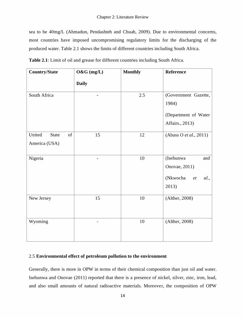
sea to be 40mg/L (Ahmadun, Pendashteh and Chuah, 2009). Due to environmental concerns,
most countries have imposed uncompromising regulatory limits for the discharging of the
produced water. Table 2.1 shows the limits of different countries including South Africa.
Table 2.1: Limit of oil and grease for different countries including South Africa.
Country/State O&G (mg/L)
Daily
Monthly Reference
South Africa - 2.5 (Government Gazette,
1984)
(Department of Water
Affairs., 2013)
United State of
America (USA)
15 12 (Abass O et al., 2011)
Nigeria - 10 (Isehunwa and
Onovae, 2011)
(Nkwocha et al.,
2013)
New Jersey 15 10 (Alther, 2008)
Wyoming - 10 (Alther, 2008)
2.5 Environmental effect of petroleum pollution to the environment
Generally, there is more in OPW in terms of their chemical composition than just oil and water.
Isehunwa and Onovae (2011) reported that there is a presence of nickel, silver, zinc, iron, lead,
and also small amounts of natural radioactive materials. Moreover, the composition of OPW
Chapter 2: Literature Review
15
from different sources or industries does vary by a certain order of magnitude. Environmental
concerns have driven the research into ensuring the quality of OPW effluent discharged into the
environment meet the stipulated standards. This is because, it is not only affecting the
surrounding location of the industry but also end up affecting the aquatic ecosystem located even
far away from the industry due to water flow which can transport such contaminants from the
original source. The main pollution challenge associated with the OPW is that it can lead to the
formation of the oil layer on top of water surface, which leads to the reduction of the light
penetration thus tempering with the process of photosynthesis which directly affect aquatic plant
growth (Abdullah, 2016). It also affects the survival of the aquatic ecosystem by hindering the
oxygen transfer by diffusion from the atmosphere to water which significantly reduce the amount
of dissolved oxygen in water (Agrawal and Sahu, 2009). Regarding discharging into municipal
wastewater treatment works (WWTW), the regulations enforce companies to pre-treat the
effluent in their schemes before channeling these industrial OPW into municipal channels. This
has been enforced in order to prevent damage to the WWTW infrastructure and any negative
disadvantageous effects on the environment and ecosystem (National guideline_Land based
influent_Discharge coastal, 2014). Therefore, it is imperative to analyze the OPW to ensure that
no negative impacts that can affect aquatic species, ecosystem, or environment. The importance
of measuring OPW is that the measurements can be used to optimize the treatment process and
can also play a role in ensuring regulatory compliance. Other benefits will include the possibility
of generation and collection of data that will allow regulators and the oil companies to establish
better environmental practices and to know precisely how much the wastewater has been
discharged and enabling the possibility to come up with the better treatment processes and
disposal.
Proper management of OPW should start from accurate measurements and estimation of the
actual volume produced. Large quantity of wastewater requires an appropriate treatment before
being discharged into the environment. It must be treated prior to being discharged into receiving
water bodies since such water usually contains dissolved and suspended matter that will temper
with the quality of water. The characteristics of the effluent in question should be defined
precisely and the quality should be examined before discharging into the aquatic environment or
to be treated and reused. This is essential for setting baseline conditions and standards.

Chapter 2: Literature Review
16
2.6 Characteristics of oil Produced Water
Quantitative assessments of the quality of the OPW are made by considering the following
parameters:
2.6.1 Water Temperature
Temperature is a very important parameter because of its influence on the water chemistry.
Normally, the rate of chemical and biological reactions increases with temperature. It is also
important to aquatic life as many biological processes such as enzymatic processes are highly
dependent on temperature which in turn affects biological activity. The temperature can be
measured using a thermometer and is expressed in °C units. Water temperature is an important
quality parameter to measure prior to the water being discharged into rivers and streams. This is
because; the temperature of water has the direct effect on all the organisms that are in it. Each
organism has its optimal temperature range to require for survival and thriving. For example,
cold water species have physiological temperature optimums <20 °C, cool water species have
physiological temperature optimums between 20 and 28 °C (Magnuson et al., 1997; Rahel and
Olden, 2008).
2.6.2 Total suspended solids (TSS)
The total suspended solids (TSS) refers to particles large enough to be retained in a filter device
of pore size 2 μm or less. TSS is usually determined by the filtration process using a vacuum
filtration unit with glass fiber filters. A high level of TSS may settle out onto a lake or stream-
bed bottom and cover aquatic organisms’ eggs, or macro-invertebrate larva (Whitman College,
2015). This coating can prevent the required oxygen transfer and result in the death of buried
organisms. Its formation is dependent primarily on physical processes driven by hydrological
factors. TSS also decreases the effectiveness of drinking water disinfection agents by allowing
the microorganisms to “hide” from disinfectants within solid aggregates (Whitman College,
2015). Hence, the turbidity or TSS is removed in drinking water treatment facilities.

Chapter 2: Literature Review
17
2.6.3 Total dissolved solids (TDS)
Total dissolved solid (TDS) refers to the total measurement for organic matter, inorganic salts as
well as other dissolved materials present in water (Butler and Ford, 2019; Gupta, 2011). It is
generally measured using gravimetric techniques by weighing the residue remaining following
evaporation of a known volume of the filtered sample. For rapid test, it can be determined using
the conductivity/TDS meters and is expressed as of mg/L. On the other hand, it can be obtained
indirectly by summing up the measured concentrations of constituents in the filtrate.
Alternatively, TDS can be estimated from conductivity (μS/cm) measurements by multiplying
with an empirical determined conversion factor ranging from 05 to 0.9. The exact factor is
determined through linear regression of repeated paired measurements of specific TDS and
conductance and it depends on the solution’s composition. Nonetheless, for most natural water
systems, 0.67 is used often when the exact conversion factor is not known (Gupta, 2011 Weiner,
2013).
2.6.4 Electrical conductivity (EC)
Electrical conductivity (EC) is the measure of the ability of the solution to conduct electric
current a property immensely dependent on the availability of ionic species (Trick, Smart and
Reeder, 2008). EC is directly proportional to a TDS measure. Basically, high levels of EC in
wastewater indicates high TDS concentration. This also implies that the concentration of ionic
solutes dissolved in water is directly proportional to the ability of an ability of an electric current
to pass through the wastewater (Atekwana et al., 2004) and therefore EC helps to indicate the
purity of water. The purer the water, the lower the EC this means that there are low levels of ions
to conduct electricity.
2.6.5 Biochemical oxygen demand (BOD)
Compounds containing organic matter can be measured in simple parameters which are
biological oxygen demand (BOD), chemical oxygen demand (COD) and total organic matter
(TOC) (Samudro and Mangkoedihardjo, 2014). BOD is an empirical test referring to the
measurements of the amount of the oxygen that the bacteria will consume while decomposing
biodegradable organic matter under aerobic conditions. It is an indirect measure of the level of
organic contamination in water and is measured in mg/L. The BOD test does not oxidize all the
organic matter present in the water but only the organic matter that are biochemically degradable

Chapter 2: Literature Review
18
during a specified incubation period which is 5 days at 20°C. BOD is set to be an indicator of
the quantum of pollution load. If the load of pollution is high therefore, there will be less DO in
water that is, greater amount of DO shall be consumed. Low values of BOD indicates relatively
pure water whereas high BOD results in harming the aquatic species (Naubi et al., 2016) hence it
is an important water quality parameter to measure.
2.6.6 Chemical oxygen demand (COD)
The chemical oxygen demand (COD) is a standard test for water which uses a strong chemical
oxygen oxidizing agent (potassium dichromate) to chemically oxidize organic matter and
inorganic chemicals in the sample of wastewater for a few hours, (normally 2 hours) under
conditions of heat and strong acid . The potassium dichromate is not specific to oxygen-
consuming chemicals either organic or inorganic and therefore, both chemicals are included in a
COD measure. It is a laboratory assay that measures the amount of organic matter
(biodegradable and non-biodegradable) in a sample and it is measured in mg/O2 equivalent /L.
The COD values of a water sample can be related to the BOD value in more or less constant
value. Since the COD test can be performed rapidly, it has an advantage (digestion in two hours)
in comparison to BOD5 (needs a minimum of five days incubation). COD test can also measure
some additional organic matter such as cellulose, which normally cannot be biologically
oxidized; hence, COD value is usually greater than that of BOD because more organic
compounds can be chemically oxidized than biologically oxidized. Therefore, it is important to
keep the COD with water quality standards because high values of COD stresses aquatic
organisms which can even lead to death (Naubi et al., 2016)
2.6.7 Total organic carbon (TOC)
TOC refers to the total content of organically bound carbon in dissolved and undissolved
compounds and it is expressed in mg/L. Organic matter present in water can be measured by use
of TOC test , which is especially applicable to small concentrations of organic matter. Organic
carbon comprises nearly all carbon compounds except those carbon species which are viewed as
inorganic (carbon dioxide, hydrogen carbonate, carbonate, cyanide, and some further examples
which are not commonly found in wastewaters). The whole sample is normally subdued to
oxidation (commonly by incineration of a known volume of the wastewater sample in the
presence of a catalyst at 900°C using CO2-free air) for detection of organic carbon in aqueous

Chapter 2: Literature Review
19
samples. It is important to check compliance of TOC because in drinking water, the organic
matter reacts with chemicals used for disinfection such as chlorine which can form disinfection
by-product which can be carcinogenic.
2.6.8 Quantification methods for organic matters
Spectrophotometry is one of the methods used for quantitative analysis in different fields
physics, chemistry, biochemistry, chemical engineering, material, and clinical applications. It
measures the amount a chemical substance absorbs light as a beam of light passes through the
sample solution. The spectroquant spectrometer has been used by many researchers for
quantitative analysis (Yang et al., 2007; Ignacio, Gernjak and Oller, 2008; Coban et al., 2015).
This is a colometric method which converts the component of a sample to be analyzed into a
coloured compound in a specific reaction by means of reagents included in the self-test kits. This
colour reaction method is an optimized approach based on standardized analytical methods. It is
optimized in terms of low working effort, easiness of use and shorter reaction times. With
spectroquant spectrophotometer method, the absorbance (which is measured by the intensity of
the color of a solution) is directly proportional to the concentration of the respective analyte.
2.6.9 Total petroleum hydrocarbons (TPH)
OPW being a complex mixture of organic and inorganic compounds has total petroleum
hydrocarbons (TPH) as one of the components and this parameter is usually important to be
analyzed including its characteristics for produced water. The effluent from refineries and
petroleum industries mainly contains oil, organic matter and other compounds (Kanu and Achi,
2011; Kulkarni and Goswami, 2015). A large family of compounds that originally come from
crude oil are known TPH. It is useful to measure the total amount of TPH at the site since it is
not practical to measure each one separately because there are many different chemicals that are
present in crude oil. The amount of TPH found in a sample is useful as a general indicator of
petroleum contamination at the site. Crude oil is used to make petroleum products and is known
to contaminate the environment (ToxFAQs, 1999; Aljuboury et al., 2017).TPH is a mixture of
chemicals and all of them contain mainly hydrogen and carbon, and such compounds are termed
as hydrocarbons. Among chemicals found in TPH are benzene, hexane, jet fuels, toluene,
naphthalene, xylems, fluorine, as well as other petroleum products and gasoline components.
However, not all of these occur in any one sample, but an individual sample will contain some or

Chapter 2: Literature Review
20
as a mixture of some of these chemicals. To prevent water pollution, it is important to monitor all
these parameters including TPH.
Sources of TPHs are many and broad; with some having their sources from the marine
environment, some from anthropogenic (pyrogenic or petrogenic) sources and some having their
origin from natural (diagenetic or biogenic) sources. Hydrocarbons which are produced by
living organisms or through biological processes for example; processes mediated by algae,
planktons, and bacteria or those involving terrestrial plants are known as biogenic sources (Tran,
Yu and Zeng, 1997; Commendatore, Esteves and Colombo, 2000). Of the hydrocarbons,
aliphatic hydrocarbons (C23-C33) are largely produced by the terrestrial plants (Kettler and
Papastavros, 2000) whereas C15, C17, and C19 (odd number) n-alkanes are produced by
biogenic marine input and mostly in low quantities (Iwegbue et al., 2016). Diagenetic sources
are those hydrocarbons which are produced as a result of a geochemical and physical changes
gone through by sediment after its initial deposition as it changes into rock and enters the marine
water usually by natural seepage (Commendatore, Esteves and Colombo, 2000). Hydrocarbons
from anthropogenic sources are mostly generated from several human activities such as
transportation, urbanization, industrialization, operations and storage, oil utilization, fishing and
shipping. Kvenvolden and Copper (2003) and Sakari et al., (2014) reported that abundance of
C16, C18, and C20 mostly suggests oil spillage from oil pipe lines and tanks used for
transferring oil from one place to another. It has been reported in literature that TPH
concentrations are extremely high in industrialized areas and spillage sites (Adeniji, Okoh and
Okoh, 2017) and amongst other factors contributing to the presence of crude oil in the marine
environment about 63% arise from atmospheric emission, urban and river runoffs, as well as
municipal and industrial discharges. Due to this, there is a need for ensuring compliance with the
environmental laws related to transportation, oil exploration and discharge into marine
environment for aquatic and human safety.
2.7 Analytical methods for the determination of TPH in water
The analytical methods for TPH involve several steps mainly sample preparation, separation, and
detection.

Chapter 2: Literature Review
21
2.7.1 Sample pre-treatment methods for TPH
Sample preparation generally refers to how a sample is treated prior to its analyses to exclude
interfering species from the sample matrix and also set free the target analytes before their
introduction to the analytical detection system. It is crucial and most important step in most
analytical procedures because otherwise the signal of the target analytes will become masked by
interfering species. Sample preparation may include sub sampling, chemical reaction with some
species, dissolution, filtration, extraction or enrichment and pre-concentration procedures.
Appropriate sampling procedure is very crucial to obtaining the correct analytical results where
the aim is to get wholly representative sample from the environmental medium where it was
collected (Weisman, 1998; ATSDR, 1999) because the aqueous sample to be analyzed can
display varying concentrations in different places at different times. For this reason, OPW being
a complex matrix it thus necessitates that a cleanup and/or enrichment of analyses be performed.
Several clean-up protocols have been reported for OPW and they include solid phase extraction
(SPE) (Yang et al., 2011; Morris, Sellaro and Sarver, 2015), solid phase micro extraction
(SPME) (Ilavsk and Hriv, 2004), vortex extraction (Suratman, 2013) and continuous liquid-
liquid extraction (LLE) (Weisman, 1998; LLE EPA 3510) .
Each of these methods has its own advantages and disadvantages. For example, SPE uses the
cartridge which contain an adsorbent such as alumina or silica in which the analytes are retained
during the SPE percolated and the analytes are then eluted with the small volume of an
appropriated organic solvents. The advantage of this method is that it uses the small volumes of
solvents and less glassware and has great efficiencies. However, with SPE the sorption process
of analytes fiber tends to compete with analytes sorption on suspended matter surface.
LLE which is a traditional solvent extraction method uses large volumes of organic solvents thus
making it uneconomical and compromises with environmentally friendly techniques as large
volumes of organic solvents will end up being disposed to the environment. Moreover, it is labor
intensive and laborious. After the LLE extraction procedure, the organic phase is collected and
concentrated prior to the instrumental analysis. In addition to the consumption of large volumes
of solvents, solvent extraction requires a lot of glassware’s (Huddleston et al., 1998; Suratman,
2013 Ahmed, Mahmoud and Mousa, 2015; Morris, Sellaro and Sarver, 2015; Adeniji, Okoh and
Okoh, 2017)

Chapter 2: Literature Review
22
2.7.2 Separation and detection methods for TPH
After the clean-up step, a mixture of analyte in the extract must be separated before their
introduction to the detection system because; when the analytes are introduced to the detector
simultaneously, they may cause interference or musk one another. Among analytical methods
used for TPH, the most commonly used include Raman spectroscopy, infrared (IR) spectroscopy,
fluorescence spectroscopy (Muthukumar et al., 2013; Okparanma and Mouazen, 2013)
gravimetry, gas chromatography with mass spectrometric detection (GC/MSD) (Reddy and
Quinn, 1999) , gas chromatography with flame ionization detection (GC/FID) (Suspes et al.,
2012), ultraviolet spectrophotometry, and immunoassay (IMA) (Okparanma and Mouazen,
2013). In addition, Reddy and Quinn, (1999) developed a Gas Chromatography-Mass
Spectrometry (GC-MS) method for measuring both the polycyclic aromatic hydrocarbons
(PAHs) and TPHs for seawater samples that were collected after the North Cape oil spill. LLE
method was employed using methyl chloride as a solvent extraction. The signal from the ion m/z
57 (C9H4+) which was a major ion in aliphatic compounds was integrated throughout the
chromatogram and used to calculate the amount of TPHs. In another study, quantification of
TPH using 5-α-androstane internal standard with a GC-MS analysis using a selected ion
monitoring (SIM) mode to improve the detection limits (Yang et al., 2011).
2.8 Gas Chromatography-Mass Spectrometry
Gas Chromatography-Mass Spectrometry (GC-MS) is a fundamental and complimentary part of
many field studies involving organic compound detection and determination. GC and MS are two
different techniques but are successfully coupled together to form GC-MS, simply because GC
can separate many volatile and semi-volatile compounds but cannot selectively detect them
whereas MS can selectively detect many compounds but not always separate them (Hussain and
Maqbool, 2014).
2.9 Evaporation principles
Evaporation is a major component and it is one aspect that is less explained of hydrological cycle
(Sudheer et al., 2002; Salarpour et al., 2014; Duffy, 2017) because it is not a simple phenomenon
to explain as it requires numerous physical, chemical and meteorological variables to be
explained. It is known as a physical process whereby a spontaneous escape of high energy

Chapter 2: Literature Review
23
molecules from liquid surface into vapor state takes place and it occurs when a liquid is not in
equilibrium with its vapor phase (Finch and Hall, 2001; Coleman, 2000) . The reverse process to
evaporation for the liquid state is known as condensation. Evaporation from a water surface has
been investigated by scientists since ancient times because it is an important process in the
hydrological cycle (Pimentel et al., 1997; Coleman, 2000; Roderick and Farquhar, 2002; Jensen,
2014). Estimates of evaporation from open water are used mainly for water balance studies to
support appraisals of applications for abstraction licenses, in wetlands and still waters
management, and has the potential to be used in modelling work in future (Finch and Hall,
2001). These estimates are increasingly required for several Environment Agency functions,
particularly Water Resources and Ecology (Kusangaya et al., 2014; Bent, 2017). It is projected
that the increase of approximately 40% in evaporation due to climate change is enough to
influence the outflow of reservoirs significantly, due to the increase in temperature (Kusangaya
et al., 2014; Bent, 2017).
Evaporation occurs at any temperature for different types of liquids and at different rates
(Vuglinsky, 2009). The rate is controlled by the energy available at the water surface and the
simplicity of the water vapor to mix in the atmosphere (Vuglinsky, 2009). Boiling differs from
evaporation; in the sense that during boiling, vapor is formed not only on the surface but also
inside the liquid and vapor bubbles go upward. Moreover, boiling occurs only at the temperature
at which the pressure of the saturated vapor in the liquid attains the value of the atmospheric
pressure. When the molecules of the liquid collide, they transfer energy to each other depending
on how they collide (Vuglinsky, 2009). When a water molecule near the water surface absorbs
enough energy to overcome the vapor pressure, it will escape in a gaseous form and enter the
surrounding air above the water. As stated by the molecular-kinetic theory, evaporation is
characterized by three phases that are interrelated and these are (i) evaporation of molecules from
the evaporating surface; (ii) the absorption of some molecules by the evaporating surface and
(iii) the diffusion of the remaining molecules into the surrounding space. Molecules in the inner
water layers are affected by the attraction of the surrounding molecules, which is similar on
average then move in any direction and at irregular intervals. Molecules at the surface water
layer are affected by less attraction of the air molecules than the molecular attraction in the inner
water layers due to the lower concentration of the air molecules. The ambient temperature, the
air humidity, solar radiation and wind speed are the major components which contribute towards

Chapter 2: Literature Review
24
the rate of evaporation (Dama-Fakir, Wurster and Toerien, 2012) .The rate of evaporation varies
depending on the geographical location and other factors which plays an important role in the
whole process of evaporation. These factors are discussed below.
2.9.1 Water quality
When soluble solids are present in the water, the vapor pressure at a particular temperature tend
to be lower compared to the pure water at the same temperature, and thus the evaporation rate
decreases with the increase of specific gravity of the solutions. Hence, the vapor pressure of sea
water with 35,000 mg/L dissolved salts is about 2 per cent less than that of pure water at the
same temperature (Finch and Hall, 2001).
2.9.2 Water depth
The effect of the water depth on the seasonal distribution of evaporation can be considerable
because of the heat storage capacity of the water body which is, determined to a large extent by
its depth.
2.9.3 Water Vapour
To have a better understanding of evaporation, it is imperative to have a better understanding of
the vapor pressure of a liquid. The average rate of movement of the molecules of a liquid
depends on the kinetic energy of the system, which is measured as temperature indirectly (Bent,
2017). The molecules of a particular liquid must have a certain characteristic minimum energy to
leave the surface of the liquid (e.g., water) therefore, the molecules with greater kinetic energy
will move away from the attraction of the other molecules into the ambient gas or air, as it
mostly is (Coleman, 2000).
2.9.4 Rainfall
Rainfall is usually measured by a device known as the rain gauge. The rainfall may alter the heat
content of a water body even though it may not cause significant changes and for this reason it is
ignored because the volume added is generally small compared to that of the water body and so
as the temperature difference.

Chapter 2: Literature Review
25
2.10 Meteorological factors affecting the rate of evaporation
The estimation of evaporation of open water set-up is generally not simple because there are a
number of factors that can affect the rate of evaporation, which mostly are the climate and the
chemistry and physio-geography of the water body and its surroundings. Several components
which have the influence on the evaporation rates are described in the following subsections.
2.10.1 Air Temperature
Generally, the rate of evaporation tends to increase with an increase in temperature. This is
because the capacity of the air mass to hold vapor molecules increases and this is also due to
increasing kinetic energy of the surface molecules which leads them to be free and become
vapor. Warmer air can hold more water vapor than colder air thus, the increase of higher
temperature leads to the higher rate of evaporation. Hence, it is difficult to evaporate a huge
amount of moisture into the air if the water is cold. As a result, a warm air and warm water
combination results into more evaporation.
2.10.2 Water temperature
Even at low temperatures, there are some water molecules having enough energy to escape and
that's why evaporation in water can occur at any temperature (yes, even if the water is in a solid
state, i.e., ice). Increase in temperature results in more molecules having kinetic energy which
lead to more water evaporation.
2.10.3 Solar radiation
Evaporation requires a lot of energy and the primary source of energy being solar radiation. Solar
radiation varies with weather conditions and the season. The incoming solar radiation warms the
water body in summer and spring. During the early winter and autumn, the incoming solar
radiation diminishes and thus the water body cools as the stored energy is released.
2.10.4 Wind speed
Generally, in nature, the incoming fresh air removes the molecules of water vapor and makes
space for other vapor molecules. Obviously the faster the rates of incoming fresh air the faster
the removal of vapor molecules. But once the wind velocity is sufficient to remove all rising
vapor molecules extra increase in wind velocity has no effect.

Chapter 2: Literature Review
26
In addition, the incoming fresh air if hot provides extra heat energy to accelerate process of
evaporation, however if the incoming fresh air is cool it reduces the evaporation rate. One of the
main functions of the wind is to remove the saturated air above the water surface during
evaporation. The wind has a major influence in maintaining the atmospheric moisture gradient to
allow consistent evaporation of the water. A water body exposed to a wind force greater than 2
m/s is considered to be dynamic (Marek and Straub, 2001). A higher evaporation rate can be
anticipated if all other factors affecting evaporation variables work together hence the
evaporation phenomena is complex. The impact from wind blowing over a water body is highly
dependent on many other variables and factors. The wind speed, flow direction and wave
breaking of the water, play significant roles in the rate of evaporation (Duan et al., 2009).
2.11 Methods used for estimation of open evaporation.
In the literature, different methods for estimating open water evaporation have been reported and
they include: mass-transfer methods (Harbeck, 1962), energy budget methods (Anderson, 1954),
radiation (Priestley and Taylor, 1972), combination methods (Penman, 1948), empirical methods
(Kohler et al., 1954), water budget methods (Shuttleworth, 1993), and temperature based
(Thornthwaite, 1948).
2.11.1 Mass or bulk transfer balance
This method of mass balance is simple in principle. However, the limitation of this method is
that it depends on the hydrological and physio geography settings. The feasibility of determining
evaporation depends primarily on the relative magnitudes of the terms. This method is not
suitable to water bodies with large flows passing through since it is very difficult to obtain a
reliable estimate whenever the evaporation is of the same order of magnitude as the errors
inherent in the measurements. In view of the possible errors, the mass balance method is unlikely
to be applicable over periods shorter than a month (Finch and Calver, 2008).
2.11.2 Energy balance method
Here in, the evaporation from a water body is estimated as the energy component required for
closing the energy budget when all the remaining components of the budget of the water body
are known, i.e. it is the residual component. Only the transfer of heat as sensible heat flux is
taken into consideration , and evapotranspiration (latent heat flux) is calculated as the residual
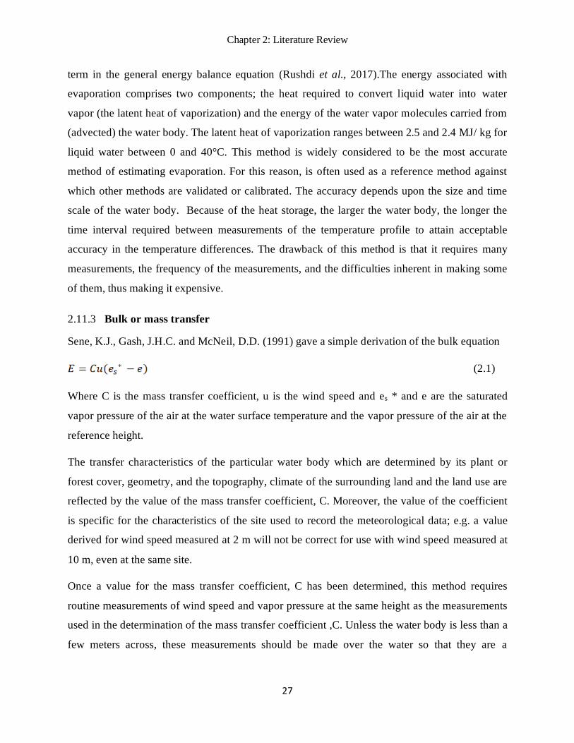
Chapter 2: Literature Review
27
term in the general energy balance equation (Rushdi et al., 2017).The energy associated with
evaporation comprises two components; the heat required to convert liquid water into water
vapor (the latent heat of vaporization) and the energy of the water vapor molecules carried from
(advected) the water body. The latent heat of vaporization ranges between 2.5 and 2.4 MJ/ kg for
liquid water between 0 and 40°C. This method is widely considered to be the most accurate
method of estimating evaporation. For this reason, is often used as a reference method against
which other methods are validated or calibrated. The accuracy depends upon the size and time
scale of the water body. Because of the heat storage, the larger the water body, the longer the
time interval required between measurements of the temperature profile to attain acceptable
accuracy in the temperature differences. The drawback of this method is that it requires many
measurements, the frequency of the measurements, and the difficulties inherent in making some
of them, thus making it expensive.
2.11.3 Bulk or mass transfer
Sene, K.J., Gash, J.H.C. and McNeil, D.D. (1991) gave a simple derivation of the bulk equation
(2.1)
Where C is the mass transfer coefficient, u is the wind speed and es * and e are the saturated
vapor pressure of the air at the water surface temperature and the vapor pressure of the air at the
reference height.
The transfer characteristics of the particular water body which are determined by its plant or
forest cover, geometry, and the topography, climate of the surrounding land and the land use are
reflected by the value of the mass transfer coefficient, C. Moreover, the value of the coefficient
is specific for the characteristics of the site used to record the meteorological data; e.g. a value
derived for wind speed measured at 2 m will not be correct for use with wind speed measured at
10 m, even at the same site.
Once a value for the mass transfer coefficient, C has been determined, this method requires
routine measurements of wind speed and vapor pressure at the same height as the measurements
used in the determination of the mass transfer coefficient ,C. Unless the water body is less than a
few meters across, these measurements should be made over the water so that they are a
Chapter 2: Literature Review
28
representative of conditions prevailing over most of the water surface. In addition, to determine *
es the average surface temperature of the water must also be measured.
When the evaporation estimates are required on hourly or daily time scales then the effects of
atmospheric stability must also be considered, however, for long-term estimates these effects can
usually be neglected (Stauffer, 1991).
2.11.4 Combination equations
The Penman (1948) and Monteith (1965) equations are also known as combination equations
since they incorporate aerodynamic water vapor mass transfer and energy balance principles.
These equations are used widely for evaporation estimation because they make use of readily
available meteorological data (Ershadi et al., 2011). Their major limitation is that they do not
take the heat storage of the water body into account if driven by net radiation data. This can be
remedied by carrying out periodic thermal surveys of the water body and inputting the available
energy, rather than the net radiation, into the equation, however, this makes the methods site
specific.
2.11.5 The equilibrium temperature method
The equilibrium temperature method is a relatively new method, which might explain why there
are few references to it in the literature. It is an attractive method because it is physically based,
uses readily available meteorological data, and takes the heat storage of the water body into
account. The only major limitation is that it assumes that the water body is uniformly mixed and
thus it does not consider thermal stratification.
2.11.6 A pan measurement
The most used instrument to measure the evaporation rate is the evaporation pan. There are
number of evaporation pans in the market for standardization of evaporation measurements.
(Klink, 2006) mentioned in his thesis that the floating evaporation pan had the ability to
reproduce water surface temperature similar to that of lake Hartwell since the major parameters
of evaporation was the water surface temperature of the lake. However, it was suggested to
investigate the impact of wind speed modifications due to the floating pan and the wooden
platform.

Chapter 2: Literature Review
29
In this project, a mostly used Class A pan was employed since it has been regarded as the
commonly used amongst farmers and water resource managers (Cobaner, 2013). There are
several methods which exist for either estimating or measuring evaporation from free water
surfaces. The use of the evaporation pans provide one of the inexpensive, simplest and most
widely used methods for evaporative losses estimations (Fekih and Saighi, 2012). Since the
Class A pan has been widely used by many researchers (Rotstayn, Roderick and Farquhar, 2006;
J and B, 2013; Gundalia and Dholakia, 2013; Izady et al., 2016; Ghorbani et al., 2018) it was
then employed for this project. Measurement of evaporation loss is recorded by measuring the
change in the water level of the pan. Water level changes can be recorded daily. Pan evaporation
is one of the most important climatic parameters in the hydrological cycle and is often applied to
estimate water requirements and terrestrial evaporation.
2.12 Application of the estimation of evaporation of open surface using different models.
Several studies have reported that, the meteorological parameters that are commonly known to
influence and affect the process of evaporation are solar radiation, temperature, relative
humidity, wind speed and atmospheric pressure (Shirgure, 2016, Sajeena et al., 2017) . To date,
many models have been developed to estimate the evaporation in different fields of study.
(Sudheer et al., 2002, Sivapragasam et al., 2009, Izady et al., 2016, Sajeena et al., 2017, Izady et
al., 2017). Simple methods such as the one reported by Stephens and Stewart, 1963, are
handicapped because they only establish a linear relationship between the variables under
investigation (Ali, 2012). This method cannot be applied for modelling OPWE because this
medium is normally highly non-linear thus prompting the search for models that are capable of
addressing this tendency of non-linearity’s in the process since wastewater cannot be directly
ascertained but only estimated depending on either the energy or water budget or mass transfer
approaches (Sudheer et al., 2002).
Another study was reported by Sudeer et al., 2002) for the prediction of evaporation using
artificial neural network (ANN) using Class A pans. The overarching objective of their study
was to assess the ANNs potential using easily available climatic data for the estimation of
evaporation and they compared their results of the Godavari Delta Irrigation project, Situated at
Dowleswaram in Andhra Pradesh, India with that of Stephens and Stewart model. The ANN
model showed to be superior to that of linear model Stephen and Steward suggested. They also

Chapter 2: Literature Review
30
find that ANN is best applicable in modelling the evaporation process with restricted data. This
suggests that the ANN model can be incorporated and become part of the module intended for
the generation of evaporation estimation data in the studies of hydrological patterns. Moreover, it
can find application in other fields including the reservoir designs, as well as water budgeting of
basins, where most other models may not be appropriate.
In another report, Sajeena et al., 2017, developed an evaporation model for their K.C.A.E.T.
campus at Tavanur in Malappuram District, using ANN technique and MATLAB software.
Monthly observations of meteorological parameters during the period February 2003 to January
2009 collected were used for the model development. The data was divided into three categories,
pre-monsoon observations, monsoon observations and post monsoon observations and each
category contained 24 observations of each parameter. The parameters considered were monthly
observation of wind speed (m/s), wet bulb temperature (°C), dry bulb temperature (°C),
maximum temperature (°C), minimum temperature (°C) and evaporation (mm). For the
development of the model, the data was divided randomly such that 70% of the observations
were placed in a training data set, 15% in a testing data set to determine the ANN models
accuracy during training in order to determine when the training should stop, and the remaining
15% for validation of the developed model. They found that the wind speed had greater influence
on the evaporation rate during all seasons. Wind speed, wet bulb temperature and dry bulb
temperature were found to be the accurate combination for the estimation of evaporation during
all the seasons with comparatively least mean squared error (MSE) and high R2 value. They
concluded that the combination the parameters mentioned above has great influence on the
evaporation during all the seasons.
Recently, Izady et al., 2017 conducted the study to investigate the ability of gene expression
programming (GEP), adaptive neuro-fuzzy inference system (ANFIS) and ANN techniques to
estimate WWE as a function of variables including wastewater physicochemical characteristics
for wastewater and clear water and climatic factors. Four Class-A pans were installed, one
containing clear water as a control and others contained three different wastewaters from
different lagoons obtained from Neishaboor municipal wastewater treatment plant in Iran. The
analysis was conducted for four months and daily CWE and wastewater evaporation (TSS, EC
and water temperature) of each pan were recorded daily. In total, 366 samples were obtained for
Chapter 2: Literature Review
31
four months, from April to July 2014. For model development, measurements from the three
lagoons were considered as “input samples” to the artificial intelligent models, and they used a
stepwise regression method to find the best input combinations from the collected variables. 366
samples were shuffled, 70% was used for testing and the remaining 30% was used for testing.
The results obtained revealed that the ANN model had an edge over the three methods, and it
demonstrated a higher accuracy when compared to dimensional analysis model using the F-test
statistic. There is still no consensus with regard to which model is the best because there are
some researchers who advocate that ANN is the best (Deswal and Mahesh, 2008, Sajeena et al.,
2017) while others have the opinion that ANFIS is the best (Kisi, Mansouri and Hu, 2017, Pour-
Ali Baba et al., 2013) and (Terzi and Kreskin, 2005 found GEP to be the best. The difference in
the opinion comes from the nature of the application and the environment where these models
were applied.
In the other study, researchers such as Izady et al., 2016 developed equations based on the
Buckingham theorem (Buckingham 1914) method using dimensional analysis for estimating
WWEs as a function of CWE. Using this approach, they measured electric conductivity (EC), air
temperature (Ta), total suspended solids (TSS), wind speed (W), and solar radiation, wastewater
temperature (Tw) using three Class A pans for the anaerobic, primary and secondary facultative
lagoons. The CWE rate was found to be less than the rate of evaporation of three wastewater
lagoons and the average evaporation rate for the wastewater of three lagoons were 40.5%, 27%
and 8.5% higher than that of CWE for the study period of four months( April-July 2016).
2.13 Development of a mathematical model
The study of modelling the rate of evaporation has been reported by various researchers and
these models have been applied in different fields. The overarching objective of this study was to
develop a model to estimate oil-produced water evaporation (OPWE) as a function of clear water
evaporation (CWE) as well as several surrounding environmental variables including TDS, TSS,
TPH, TOC, oil-produced temperature (Topw), EC, COD, BOD and the climatic variables
including air temperature (Ta), Wind speed (W) and solar radiation (R). Generally, OPWE is
highly nonlinear in nature, thus prompting the search for models that can address this tendency.
In addition, modelling the evaporation rate is important since it cannot be directly ascertained but
only estimated depending on either the energy or water budget or mass transfer approaches

Chapter 2: Literature Review
32
(Sudheer et al., 2002). A very powerful and general tool for use in analyzing and understanding
problems in science and engineering is known as dimensional analysis. It involves a dimensional
model analysis whereby a large group of variables which arise in practical problems are reduced
to its simplest algebraic form. This method is a concept of similarities and functional relations,
and it is presented amongst them by a criterion equation. In modelling, the aim is to reduce the
number of independent variables to the simplest form and to generalize the results thereof. This
method can be effective more especially if mathematical model of the investigated process is
unknown. Moreover, dimensional analysis deals with the conversion of physical quantities into
other various fundamental sets of measuring units, the conversion of measuring units and other
procedures. Dimensional model analysis becomes a powerful tool mostly if a complete
mathematical model of the investigated process is unknown.
2.14 Buckingham theorem
With the aim of providing a cost-effective and acceptable solutions to attain the model to predict
compliance of the OPW; dimensional analysis based on Buckingham theorem seems to be the
best method to use for model development. Dimensional analysis based on Buckingham
theorem has been implemented by different researchers (Reddy and Reddy, 2014; Izadi et al.,
2016; Polverino et al., 2019; Misic, Najdanovic-lukic and Nesic, 2010). A physical quantity may
have dimensions or be dimensionless. The physical quantities may have dimensions (that is,
dimensional) or dimensionless. The numerical value of the quantity depends on the measuring
units of the system. Following the Buckingham theorem, the physical quantities are expressed
in International System of units (SI) then converted to its dimensions for example, the SI units of
speed of light are meter per second (m/s) and it dimensions are length per time (L/T) . Since
dimensional analysis is a method of reduction of complex dependence of the physical quantity to
its simplest form, it is important to the select of the parameters that have an influence/effect on
the experimental data being investigated. The square brackets [] are used to show the physical
quantity of the system, example, if we are interested in the speed of light (m/s) then its
dimensions will be written as [L/T].

Chapter 2: Literature Review
33
The main functions of the Buckingham theorem are as follows:
1. Select pertinent variables (n)
2. Write the function relation (for example, )
3. Select the repeating variables (dependent variables cannot be chosen as the repeating
variable, the selected variables should contain all the m dimensions (M, L, T, and etc.)
and the non dimensionless parameters were not selected as repeating parameters.)
4. Calculate the number of terms that the physical relationship can be reduced to (n-m).
5. Write the terms by combining the repeating variables with each of the non-repeating
variables.
6. Solve the equations obtained from step 5
7. Write the functional relationship in terms of the pi terms (
2.15 Conclusion
According to new reports by the WHO and UNICEF (United Nations International Children's
Emergency Fund), 2.1 billion people lack access to clean water and about 4.5 billion lack safely
to adequate sanitation globally. This is due to the dwindling of the sources of freshwater and also
the water pollution that plays an important role in the water crisis worldwide by reducing the
freshwater resources quantity available to humans and the ecosystems (Aniyikaiye et al., 2019).
Countries such as China, India, South Africa (and other many African counties), as well as the
whole of developing and developed countries are having a shortage in the reliable and
sustainable supply of freshwater (Ganoulis, 2009). There has been a rapid industrial development
in South Africa in the past century and due to this development, there has been an increase in the
complex toxic effluents that have been reported in the environment. Some of the chemicals and
processes used by industries used to treat produced water effluent are toxic and may even lead to
secondary pollution which is one of the sources of the contamination of freshwater sources.
Therefore, there is a need for a development of a model to predict the compliance of the OPW
using their evaporation patterns

Chapter 2: Literature Review
34
2.16 References
Abass O, A., Jameel A.T. Muyubi, S. Karim, M.A.I. and Alam, M.Z. (2011) ‘Removal of Oil
and Grease as Emerging Pollutants of Concern (EPC) in Wastewater Stream’, IIUM Engineering
Journal, 12(4), pp. 161–169. doi: 10.31436/iiumej.v12i4.218.
Abdullah BT, S. (2016) Removal of oil and grease from agro-food industrial effluent using
serratia marcescens sa30 and its kinetic study shakila bt abdullah universiti teknologi malaysia.
Universiti Teknologi Malaysia.
Adeniji, A. O., Okoh, O. O. and Okoh, A. I. (2017) ‘Analytical Methods for the Determination of
the Distribution of Total Petroleum Hydrocarbons in the Water and Sediment of Aquatic
Systems : A Review’, Journal of Chemistry, pp. 13.
Adeniyi, A. A., Yusuf, K. A. and Okedeyi, O. O. (2008) ‘Assessment of the exposure of two fish
species to metals pollution in the Ogun river catchments, Ketu, Lagos, Nigeria’, Environmental
Monitoring and Assessment, 137(1–3), pp. 451–458. doi: 10.1007/s10661-007-9780-5.
Adewuyi, G. O. and Olowu, R. a (2012) ‘Assessment of Oil and Grease , Total Petroleum
Hydrocarbons and Some Heavy Metals in Surface and Groundwater Within the Vicinity of Nnpc
Oil Depot in Apata , Ibadan Metropolis , Nigeria’, International Journal of Research and
Reviews, 13(October), pp. 166–174.
Agrawal, A. and Sahu, K.K. (2009). An Overview of the Recovery of Acid from Spent Acidic
Solutions from Steel and Electroplating Industries. Journal of Hazardous Materials, 171, 61-75.
Ahmadun, F., Pendashteh, A. and Chuah, L. (2009) ‘Review of technologies for oil and gas
produced water treatment’, Journal of Hazardous Materials, 170, pp. 530–551. doi:
10.1016/j.jhazmat.2009.05.044.
Ahmed, E., El-Sayed, A. M. A. and El-Saka, H. A. A. (2007) ‘Equilibrium points, stability and
numerical solutions of fractional-order predator-prey and rabies models’, Journal of
Mathematical Analysis and Applications, 325(1), pp. 542–553. doi: 10.1016/j.jmaa.2006.01.087.
Ahmed, O. E., Mahmoud, S. A. and Mousa, A. E. R. (2015) ‘Aliphatic and Poly-Aromatic
Hydrocarbons Pollution at the Drainage Basin of Suez Oil Refinery Company’, Current Science

Chapter 2: Literature Review
35
International, 4(1), pp. 27–44.
Al-Kaabi, M. A., Al-Ghouti, M.A. Mohammed, Y.M.A and Ahmeed,T. (2019) ‘An integrated
approach for produced water treatment using microemulsions modified activated carbon’,
Journal of Water Process Engineering. Elsevier, 31, pp. 1–7. doi: 10.1016/j.jwpe.2019.100830.
Ali, M. (2012) ‘Modelling Pan Evaporation Using Genetic Programming. University of Tabriz
Texas A and M University of Civil Engineering University of Maragheh’, 8, pp. 15–36.
Aljuboury, D. A. D. A., Palaniandy, P. Abdul, A.H.B and Feroz. S (2017) ‘Treatment of
petroleum wastewater by conventional and new technologies - A review’, Global Nest Journal,
19(3), pp. 439–452. doi: 10.30955/gnj.002239.
Alther, G. (2008) ‘Cleaning wastewater: Removing oil from water with organoclays’, Filtration
and Separation, 45(3), pp. 22–24. doi: 10.1016/S0015-1882(08)70057-0.
Alzahrani, S. and Mohammad, A. W. (2014) ‘Challenges and trends in membrane technology
implementation for produced water treatment: A review’, Journal of Water Process Engineering.
Elsevier Ltd, 4, pp. 107–133. doi: 10.1016/j.jwpe.2014.09.007.
Anderson, E.R. (1954) ‘Energy-Budget Studies. In: Water loss Investigations: Lake Hefner
Studies’. Technical Report, pp. 71-119.
Aniyikaiye, T. E., Oluseyi, T. Odiyo, J.O. and Edokpayi, J.N. (2019) ‘Physico-Chemical
Analysis of Wastewater Discharge from Selected Paint Industries in Lagos , Nigeria’,
International Journal oF Environmental Research and Public Health, 16, pp. 1–17. doi:
10.3390/ijerph16071235.
Atekwana, E.A., Atekwana, E.A. Rowe, R.S. Werkema Jr, D.D. and Legall, F.D (2004) ‘The
relationship of total dissolved solids measurements to bulk electrical conductivity in an aquifer
contaminated with hydrocarbon’, Journal of Applied Geophysics, 56, pp. 281–294. doi:
10.1016/j.jappgeo.2004.08.003.
Bent, D. (2017) A Comparison Of Brine Evaporation Rates Under Controlled Conditions In A
Laboaratory.
Butler, B. A. and Ford, R. G. (2019) ‘Evaluating relationships between total dissolved solids

Chapter 2: Literature Review
36
(TDS) and total suspended solids (TSS) in a mining-influenced watershed’, Mine Water
Environ., 37(1), pp. 1–12. doi: 10.1007/s10230-017-0484-y.Evaluating.
Coban, O., Kuschk, P. Wells, N.S Strauch, G. and Knoeller, K. (2015) ‘Microbial nitrogen
transformation in constructed wetlands treating contaminated groundwater’, Environ Sci Pollut
Res, 22(3), pp. 12829–12839. doi: 10.1007/s11356-014-3575-3.
Cobaner, M. (2013). ‘Reference Evapotranspiration Based on Class A Pan Evaporation Via
Wavelet Regression Technique’. Irrigation Science., pp.119-134
Coleman, M. (2000) Review and Discussion on the Evaporation Rate of Brines,
Members.Iinet.Net.Au. Available at:
http://members.iinet.net.au/~actis/evaporation_rate_of_brines.pdf.
Commendatore, M. G., Esteves, J. L. and Colombo, J. C. (2000) ‘Hydrocarbons in coastal
sediments of Patagonia, Argentina: Levels and probable sources’, Marine Pollution Bulletin,
40(11), pp. 989–998. doi: 10.1016/S0025-326X(00)00042-4.
Dama-Fakir, P., Wurster, A. and Toerien, A. (2012) Field testing to determine the evaporation
rate of brine solutions formed during the membrane treatment of mine- water.
Department of Water Affairs. (2013) Revision of general authorisations in terms of Section 39 of
the National Water Act, 1998 (Act No. 36 of 1998), No. 665. Government Gazette No. 36820, 6
September. Department of Water Affairs, Pretoria, South Africa.
Deswal, S. and Mahesh, P. (2008) ‘Artificial neural network based modeling of evaporation
losses in reservoirs’, World Academy of Science, Engineering and Technology, 39, pp. 279–283.
Available at:
http://citeseerx.ist.psu.edu/viewdoc/download?doi=10.1.1.193.2639&rep=rep1&type=
pdf.
Duan, Z., Martin, J.L. Mcanally, W.H. and Stockstill, R.L. (2009). ‘Combined Effects of Wind
and Streamflow on Gas-Liquid Transfer Rate’. Journal of Environmental Engineering
Duffy, C. J. (2017) ‘The terrestrial hydrologic cycle: an historical sense of balance’, Wiley
Interdisciplinary Reviews: Water, 4, p. 1216. doi: 10.1002/wat2.1216.

Chapter 2: Literature Review
37
Ershadi, A., McCabe, M.F. Evans, J.P. and Walker, J.P. (2011) ‘Evaluation of Energy Balance,
Combination, and Complementary schemes for estimation of evaporation’, IAHS-AISH
Publication, 344, pp. 52–56.
Fekih, M. and Saighi, M. (2012) ‘Measurement and Estimation of Evaporation from Water
Surfaces : Application to Dams in Arid and Semi Arid Areas in Algeria’, International Journal
of Mathematical , Computational, Physical , electrical and Computer Engineering, 6(8), pp.
905–908.
Finch, J. and Calver, A. (2008) ‘Methods for the quantification of evaporation from lakes’, in
Methods for the quantification of evaporation from lakes prepared, pp. 1–23.
Finch, J. W. and Hall, R. L. (2001) Estimation of Open Water Evaporation.
Ganoulis, J. (2009) Risk Analysis of Water Pollution. 2nd ed.; WILEY-VCH Verlag GmbH & Co.
KGaA: Weinheim, Germany, 2009;
Ghorbani, M. A., Kazempour,R. Chau, K. Shamshirband, S. Ghazvinei, T.P. (2018) ‘Mechanics
Forecasting pan evaporation with an integrated artificial neural network quantum-behaved
particle swarm optimization model : a case study in’, Engineering Applications of Computational
Fluid Mechanics, 12(1), pp. 724–737. doi: 10.1080/19942060.2018.1517052.
Government Gazette (1984) Requirements for the Purification of Wastewater or Effluent.
Gazette No 9225, Regulation No 991, 18 May.
Gundalia, M. and Dholakia, M. (2013) ‘Modelling pan evaporation using mean air temperature
and mean pan evaporation relationship in middle south Saurashtra Region’, International
Journal of Water Resources and Environmental Engineering Review, 5(11), pp. 622–629. doi:
10.5897/IJWREE2013.0426.
Gupta, S. K. (2011) Morden hydrology and Sustainable water Development.
Harbeck, G. E. (1962) ‘A practical field technique for measuring reservoir evaporation utilizing
mass-transfer theory’ Geological Survey Professional Paper 272-E. US Government Printing
Office, Washington, D.C. pp. 101–105.
Huddleston, J. G., Willauer, H.D. Swatloski, R.P. Visser , A.E and Rogers , R.D (1998) Room

Chapter 2: Literature Review
38
temperature ionic liquids as novel media for ‘ clean ’ liquid – liquid extraction.
Hussain, S. Z. and Maqbool, K. (2014) ‘GC-MS: Principle, Technique and its application in
Food Science’, International Journal of Current Science, 13, pp. 116–126.
Ignacio, M., Gernjak, W. and Oller, I. (2008) ‘Coupled solar photo-Fenton and biological
treatment for the degradation of diuron and linuron herbicides at pilot scale’, Elsevier, 72, pp.
622–629. doi: 10.1016/j.chemosphere.2008.02.043.
Igunnu, E. T. and Chen, G. Z. (2014) ‘Produced water treatment technologies’, International
Journal of Low-Carbon Technologies, 9, pp. 157–177. doi: 10.1093/ijlct/cts049.
Ilavsk, J. and Hriv, J. (2004) ‘Determination of Petroleum Hydrocarbons in Water By
Microextraction And Capi- Llary Gas Chromatography’, Slovak Journal of Civil Engineering, l,
pp. 13–17.
Isehunwa, S. and Onovae, S. (2011) ‘Evaluation of water discharge in the Nigeria-Delta’,
Journal of Engineering and Applied Sciences, 6(8), pp. 66–72.
Iwegbue, C. M., Aganbi, E. Obi, G. Osakwe, S.A, Eguvbe, P.M. Ogala, J.E. and Martincigh,
S.B. (2016) ‘Aliphatic hydrocarbon profiles in sediments of the Forcados River, Niger Delta,
Nigeria’, Environmental Forensics. Taylor & Francis, 17(2), pp. 144–155. doi:
10.1080/15275922.2016.1163620.
Izady A., Abdalla, O., Sadeghi, M., Majidi, M,. Karimi, A., and Chen M., (2016). Novel
Approach to Modeling Wastewater Evaporation Based on Dimensional Analysis, Water
Resources Management. Water Resources Management, 30, pp. 2801–2814. doi:
10.1007/s11269-016-1324-8.
Jamaly, S., Giwa, A. and Hasan, S. W. (2015) ‘Recent improvements in oily wastewater
treatment: Progress, challenges, and future opportunities’, Journal of Environmental Sciences,
37, pp. 15–30. doi: 10.1016/j.jes.2015.04.011.
Jensen, M. E. (2014) ‘Estimating evaporation from water surfaces’, pp. 1–28.
Kanu, I. and Achi, O. (2011) ‘Industrial Effluents and Their Impact on Water Quality of
Receiving Rivers in Nigeria’, Journal of Applied Technology in Environmental Sanitation, 1(1),

Chapter 2: Literature Review
39
pp. 75–86.
Kettler, R. and Papastavros, E. (2000) ‘Preliminary Results of Bitumen and Whole-Rock
Elemental Analyses of CRP-2/2A, Victoria Land Basin, Antarctica’, Papers in the Earth and
Atmospheric Sciences, 7(3), pp. 361–367.
Kisi, O., Mansouri, I. and Hu, J. W. (2017) ‘A New Method for Evaporation Modeling: Dynamic
Evolving Neural-Fuzzy Inference System’, Advances in Meteorology, 2017. doi:
10.1155/2017/5356324.
Klink, M. (2006) Evaporation Estimation Using a Floating Pan.
Kohler M. A (1954) ‘Lake and panevaporation.Water-loss investigations:lake Hefner studies’
technical report. US Geol Surv Prof Pap 269, pp.127–149
Kulkarni, S. J. and Goswami, A. K. (2015) ‘A Review on Wastewater Treatment for Petroleum
Industries and Refineries’, International Journal of Scientific Research in Science, Engineering
and Technology, 1(3), pp. 280–283.
Kvenvolden, K. and Copper, C. (2003) ‘Natural seepage of crude oil into the marine
environment’, pp. 140–146. doi: 10.1007/s00367-003-0135-0.
Machín-Ramírez, C., Okoh, A.I. Morales, D. Mayolo-Deloisa, Quintero, R. and Treojo-
Hernandez, T.R. (2008) ‘Slurry-phase biodegradation of weathered oily sludge waste’,
Chemosphere, 70(4), pp. 737–744. doi: 10.1016/j.chemosphere.2007.06.017.
Magnuson, J. J., Webster, R. A. Assel, C. J. Bowser, P. J. Dillon,J. G. Eaton, H. E. Evans, E. J.
Fee, R. I. Hall, L. R. Mortsch, D. W. Schindler And F. H. Quinn (1997) ‘Potential effects of
climate changes on aquatic systems : laurentian great lakes and precambrian shield region’,
Hydrological Processes, 11, pp. 825–871.
Marek, R., and Straub, J. (2001). ‘Analysis of the Evaporation Coefficient and the Coefficient
Condensation of Water’. International Journal of Heat and Mass Transfer. pp.39-53.
Misic, T., Najdanovic-lukic, M. and Nesic, L. (2010) ‘Dimensional analysis in physics and the
Buckingham theorem’, European Journal of Physiscs, 893(31), pp. 893–906. doi: 10.1088/0143-
0807/31/4/019.

Chapter 2: Literature Review
40
Monteith, J. (1965) ‘Evaporation and the environment. In: 19th Symposium of the Society of
Experimental Biology’. Cambridge: Cambridge University Press, pp. 205-234.
Morris, J., Sellaro, R. and Sarver, E. (2015) ‘Residual diesel range organics in process waters
from laboratory’, Oficial publication of the Society for Mining, Metallurgy & Exploration Inc.,
pp. 67–73.
Muthukumar, A., Idayachandiran, G. Kumaresan, S. Kumar, T. A. and Balasubramanian, T.
(2013) ‘Petroleum Hydrocarbons ( PHC ) in Sediments of Three Different Ecosystems from
Southeast Coast of India’, International Journal of Pharmaceutical & Biological Archives, 4(3),
pp. 543–549.
Munirasu, S., Haija, M. A. and Banat, F. (2016) ‘Use of membrane technology for oil field and
refinery produced water treatment - A review’, Process Safety and Environmental Protection.
Institution of Chemical Engineers, 100, pp. 183–202. doi: 10.1016/j.psep.2016.01.010.
Nationalguideline_Landbasedinfluent_Dischargecoastal (2014).
Naubi, I., Zardari, N.S. Shirazi1, S. M. Farahen, N. Ibrahim, B. and Baloo. L.(2016)
‘Effectiveness of Water Quality Index for Monitoring Malaysian River Water Quality’, 25(1),
pp. 1–9. doi: 10.15244/pjoes/60109.
Nkwocha, A., Ekeke, I.C. Kamen, F.L. and Oghome, P.I. (2013) ‘Quality Assessment of Effluent
Discharges from Vegetable oil Plant’, Ethiopian Journal of Environmental Studies and
Management, 6, pp. 717–723. doi: 10.4314/ejesm.v6i6.2s.
Okparanma, R. N. and Mouazen, A. M. (2013) ‘Determination of total petroleum hydrocarbon
(TPH) and polycyclic aromatic hydrocarbon (PAH) in soils: A review of spectroscopic and
nonspectroscopic techniques’, Applied Spectroscopy Reviews, 48(6), pp. 458–486. doi:
10.1080/05704928.2012.736048.
Penman, H.L. (1948) ‘Evaporation in nature’. Report on Progress in Physics 11, pp.366-388.
Pimentel, D., Houser, J. Preiss, E. White, O. Fang, H. Mesnick, L. Brasky, T. Tariche, S.
Schreck, J. and Alpert, S. (1997) ‘Water Resources : Agriculture , the Environment , and Society.
An assessment of the status of water resources’, Bioscience, 47(2), pp. 97–106.

Chapter 2: Literature Review
41
Polverino, P., Bovea, G. Sorrentinoa,M. Pianesea, C. and Berettab, D. (2019) ‘Advancements
on scaling-up simulation of Proton Exchange Membrane Fuel Cells impedance through
Buckingham Pi theorem’, Applied Energy. Elsevier, 249, pp. 245–252. doi:
10.1016/j.apenergy.2019.04.067.
Pour-Ali Baba, A., Shiri, J. Kisi, O. Fard, A.F. Kim, S. and Amini, R. (2013) ‘Estimating daily
reference evapotranspiration using available and estimated climatic data by adaptive neuro-fuzzy
inference system (ANFIS) and artificial neural network (ANN)’, Hydrology Research, 44(1), p.
131. doi: 10.2166/nh.2012.074.
Priestley, C.H.B. and Taylor, R.J. (1972) ‘On the assessment of surface heat flux and
evaporation using large-scale parameters ’. Monthly Weather Review 100, pp.81-92.
Rahel, F. J. and Olden, J. D. (2008) ‘Assessing the Effects of Climate Change on Aquatic
Invasive Species’, 22(3), pp. 521–533. doi: 10.1111/j.1523-1739.2008.00950.x.
Reddy, C. M. and Quinn, J. G. (1999) ‘GC-MS analysis of total petroleum hydrocarbons and
polycyclic aromatic hydrocarbons in seawater samples after the North Cape oil spill’, Marine
Pollution Bulletin, 38(2), pp. 126–135. doi: 10.1016/S0025-326X(98)00106-4.
Reddy, G. M. and Reddy, V. D. (2014) ‘Theoretical Investigations on Dimensional Analysis of
Ball Bearing Parameters by using Buckingham Pi-Theorem’, Procedia Engineering. Elsevier
B.V., 97, pp. 1305–1311. doi: 10.1016/j.proeng.2014.12.410.
Roderick, M. L. and Farquhar, G. D. (2002) ‘The Cause of Decreased Pan Evaporation over the
Past 50 Years’, 298, pp. 1410–1412.
Røe Utvik, T. I. (1999) ‘Chemical characterisation of produced water from four offshore oil
production platforms in the North Sea’, Chemosphere, 39(15), pp. 2593–2606. doi:
10.1016/S0045-6535(99)00171-X.
Rotstayn, L. D., Roderick, M. L. and Farquhar, G. D. (2006) A simple pan-evaporation model for
analysis of climate simulations : Evaluation over Australia. doi: 10.1029/2006GL027114.
Rushdi, A. I., Al-Shaikh, I. El-Mubarak, A.H. Alnaimi, H.A.J.A. Al-Shamary, N. Hassan, H.M
and Assal, M.A. (2017) ‘Characteristics and sources of anthropogenic and biogenic
hydrocarbons in sediments from the coast of Qatar’, Marine Pollution Bulletin. Elsevier, 124(1),

Chapter 2: Literature Review
42
pp. 56–66. doi: 10.1016/j.marpolbul.2017.07.014.
Sajeena, S., Gayathry, V. A. and Sharmina, V. K. (2017) ‘Estimation of Pan Evaporation Using
Artificial Neural Networks – A Case Study’, 6, pp. 3052–3065.
Sakari, M., Hsia, B.S. Tahir, R. Rafiq,S. Nahavandi, M.D.S. Annammala, K.V. Soon, Z.Y and
Yi, A.L.J ‘Estuary and Sea-associated Wetlands as Final Sink for Organic Pollutants : A Case
Study in Sabah , Malaysia’, International Journal of Environment and Bioenergy, 9(1), pp. 1–16.
Salarpour, M., Yusop, Z. Jajamezadeh, M. and Yusof, F. (2014) ‘Development of generalized
feed forward network for predicting annual flood (Depth) of a tropical river’, Sains Malaysiana,
43(12), pp. 1865–1871. doi: 10.17576/jsm-2014-4312-07.
Samudro, G. and Mangkoedihardjo, S. (2014) ‘Review on BOD , COD and BOD / COD ratio : a
triangle zone for toxic , biodegradable and stable levels, International Journal of Academic
Research, 2(4), pp. 235–239.
Sene, K.J., Gash, J.H.C. and McNeil, D.D. (1991) ‘Evaporation from a tropical lake: comparison
of theory with direct measurements’, Journal of Hydrology. 127, pp.193-217
Shirgure, P. (2016) ‘Evaporation Modeling with Artificial Neural Network - A Review Review
article Evaporation modeling with artificial neural network : A review’, 2, pp. 73–84.
Shuttleworth, W.J. (1993) Evaporation. In: Maidment, D.R., (Ed.) Handbook of Hydrology, New
York: McGraw-Hill.
Silva, R. de C. F. S., Almeida, D.G. Rufuno, R.D. Luna, J.M. Santos, V.A. Sarubbo, V.A and
Leonie, A.S.(2014) ‘Applications of biosurfactants in the petroleum industry and the remediation
of oil spills’, International Journal of Molecular Sciences, 15(7), pp. 12523–12542. doi:
10.3390/ijms150712523.
Stauffer, R.E. (1991) ‘Testing lake energy budget models under varying atmospheric stability
conditions’. Journal of Hydrology. 128, pp.115-135.
Sudheer, K. P., Gosain, A.K. Mohana R.D. and Saheb, S.M. (2002) ‘Modelling evaporation
using an artificial neural network’, Hydrological Processes, 16, pp. 3189–3202.
Suspes, A., Roa, S. and González, C. and Castro, H.E. (2012) ‘Total Petroleum Hydrocarbons By

Chapter 2: Literature Review
43
Gas Chromatography in Colombian Waters and Soils’, American Journal of Environmental
Science, 8(4), pp. 396–402. doi: 10.3844/ajessp.2012.396.402.
Suratman, S. (2013) ‘Distribution of Total Petrogenic Hydrocarbon in Dungun River Basin ,
Malaysia’, Oriental Journal of Chemistry, 29(1), pp. 77–80.
Thomas, K. V., Langford, K. Perterson, K. Smith, A.J and Tollefson, K.E. (2009) ‘Effect-
directed identification of naphthenic acids as important in vitro xeno-estrogens and anti-
androgens in North Sea offshore produced water discharges’, Environmental Science and
Technology, 43(21), pp. 8066–8071. doi: 10.1021/es9014212.
Thornthwaite, C. W., 1948: An approach towards a rational classification of climate.Geography
Review, 38, pp. 55–94.
Todd, G. D., Chessin, R. L. and Colman, J. (1999) Toxilogical Profile for Total Petroleum
Hydrocarbons (TPH). Public Health.
ToxFAQs, A. for T. S. and D. R. (1999) Total Petroleum Hydrocarbons (Tph) Agency For Toxic
Substances And Disease Registry Toxfaqs. Available at:
http://www.atsdr.cdc.gov/toxfaq.html%0Ahttps://www.atsdr.cdc.gov/toxfaqs/tfacts123.pdf.
Tran, K. T., Yu, C. and Zeng, E. Y. (1997) ‘Organic Pollutants In The Coastal Environment Off
San Diego , California .Petrogenic And Biogenic Sources Of Aliphatic Hydrocarbons’,
Environmental Toxicology and Chemistry, 16(2), pp. 189–195.
Trick, J., Smart, M. and Reeder, S. (2008) ‘Contaminated groundwater sampling and quality
control of water analyses Source’, Environmental Geochemistry, pp. 1–20.
Varjani S, Kumar G, Rene ER (2019) ‘Treatment of wastewater from petroleum industry: current
practices and perspectives’, Environmental Science and Pollution Research, pp. 1–9. doi:
10.1007/s11356-019-04725-x.
Vuglinsky, V. S. (2009) Evaporation from open water surface and groundwater, hydrological
cycle.
Weiner, E. R. (2013) ‘Aquatic Chemistry’, in Applications of Environmental Aquatic Chemistry:
A Practical Guide 3rd. CRC Press; Florida, pp. 1–79.

Chapter 2: Literature Review
44
Weisman, W. (1998) Analysis of Petroleum Hydrocarbons in Environmental Media.
Whitman College (2015) ‘Total Suspended Solids in Water Samples’ Available at:
https://www.whitman.edu/chemistry/edusolns_software/TSSBackground.pdf.
WHO & UNICEF Joint press release 2017, 2.1 Billion People Lack Safe Drinking Water at
Home, More Than Twice as Many Lacks Safe Sanitation. Available online:
https://www.unicef.org/media/media_96632.html (accessed on 21 August 2019).
Yang, Y., Charles, R.B. Sadriesh, N. May, J.C. Grosso, A.V.D Lyon, R.C and Faustino, P.J.
(2007) ‘Validation of an in vitro method for the determination of cyanide release from ferric-
hexacyanoferrate : Prussian blue’, Journal of Pharmaceutical and Biomedical Analysis, 43, pp.
1358–1363. doi: 10.1016/j.jpba.2006.11.010.
Yang, Z., Yang, C. Wang, Z. Hellebone, B. Landriault, M. and Brown, C.E. (2011) ‘Oil
fingerprinting analysis using commercial solid phase extraction (SPE) cartridge and gas
chromatography-mass spectrometry (GC-MS)’, Analytical Methods, 3(3), pp. 628–635. doi:
10.1039/c0ay00715c.
Yu, L., Han, M. and He, F. (2017) ‘A review of treating oily wastewater’, Arabian Journal of
Chemistry, 10, pp. S1913–S1922. doi: 10.1016/j.arabjc.2013.07.020.

45
CHAPTER 3 : RESEARCH METHODOLOGY
This chapter narrates the details of the samples and sampling procedures, sample preparation
protocols, materials and reagents used in pursuit of the research objectives for this project as well
as the experimental protocols used to generate the data that provided the results reported in this
dissertation.
3.1 Materials and methods
3.1.1 Chemicals and materials
A surrogate standard of 1-chlorooctadecane (96%) was purchased from Sigma-Aldrich
(Johannesburg, South Africa).The solvents used for liquid-liquid extraction (LC-MS grade ethyl
acetate, LC-MS grade dichloromethane and LC-MS grade hexane), cell test kits for biological
oxygen demand (BOD), chemical oxygen demand (COD) and total organic carbon (TOC) were
purchased from Merck-Millipore (Darmstadt, Germany). Sodium sulphate salt and silica gel
were purchased from Sigma-Aldrich (Johannesburg, South Africa).
3.1.2 Apparatus
Stainless steel bailer sampler was used for sampling at the oil depot. A graduated measuring
device (Figure 3.2b) was used to measure the evaporated water daily from the pans. Separating
funnel was used for liquid-liquid extraction (LLE) for total petroleum hydrocarbons (TPH)
analysis, A vacuum filtration unit was used in the procedures for total suspended solids (TSS).
3.1.3 Instrumentation
(For BOD5) analysis, the water bath was set at 20°C and used for incubation during 5-day
biological oxygen demand. A Merck-Millipore UV-VIS Spectrophotometer Pharos 300
Spectroquant® was used to assess chemical oxygen demand (COD), total organic carbon (TOC),
and as well as BOD5. The thermo reactor was used for sample digestion for the COD, BOD5 and
TOC analysis. The TurboTax instrument was used to dry the extracted TPH. GCxGC-TOF-MS
was used to identify and quantify the TPH from the collected samples. Multi-parameter probe,
Accsen from XS (Carpi MO, Italy) field meter was used to measure the physical parameters

Chapter 3: Research Methodology
46
including electrical conductivity (EC), total dissolved solids (TDS), clear water and oil-
produced water temperatures (Tcwe) and (Topw) respectively.
3.2 Class A evaporation pan and field deployment
3.2.1 Fabrication of Class A pan
The Class A pan was constructed at the UNISA’s Science Campus workshop using stainless steel
and has a cylindrical shape (Figure 3.1a) The diameter of the Class A evaporation pan was 12.1
cm and height 25.4 cm. To enhance air circulation under the set-up, the pan was placed over the
wooden frame 15 cm from the ground.
Figure 3.1: (a) Constructed evaporation pan (Izady et al., 2016) (b) Class A pans filled with
clear water (c) Class A pan filled with oil produced water installed at the field for this work.

Chapter 3: Research Methodology
47
3.3 Field Measurements
3.3.1 Evapoartion rate measurements principle
Two Class A pans were deployed at the field at an oil depot (Figure 3.2 a), one filled with a
known volume of oil produced water (OPW) and the second was filled with the same volume of
clear water. The clear water pan was meant to be the reference/control setup for measuring the
evaporated water daily. The pans were installed at the site within an oil depot. The water was
allowed to evaporate for 24 hours then measurements were recorded for the water depth in the
pans using the water finder on the graduated measuring device (Figure 3.2 b). The difference
between the two measured water depths for two successive days was then calculated by
subtraction (Previous day level/depth minus today’s depth/level) to give the magnitude of
evapoaration Ep ( in millimeter units).
Figure 3.2: (a) Two Class A pans filled with clear water and effluent (OPW) for daily
evaporation rates. (b) Measuring device and the water finder to measure the water depth.

Chapter 3: Research Methodology
48
3.3.2 Measurements of environmental parameters in the field
A Multi-parameter probe, Accsen from XS (Carpi MO, Italy) was permanently deployed at the
field and was used for measuring water temperatures, electrical conductivities (EC) and total
dissolved solids (TDS). The multimeter probe was soaked with 1% hydrochloric acid (HCl) and
then rinsed with deionized water three times prior to each measurement to avoid any possibility
of cross-contamination.
3.3.3 Measurements of climatic parameters
Climatic parameters including solar radiation (R), wind speed (W), and air temperature (Ta)
were measured by a mini portable weather station (Figure 3.3) which was also deployed
permanently in the field. The portable mini weather station included light intensity meter, wind
vane, anemometer, temperature probe for measuring air temperature and rain gauge all in-built
in the station. The rain gauge was essential in correcting the water levels during rainy days.
Figure 3.3: Portable mini-weather station installed at the oil depot.

Chapter 3: Research Methodology
49
3.4 Description of oil depot works
The oil depot where OPW was collected, distribute petrol, diesel, and gas to various filling
stations. The influent wastewater at the depot is subjected to mechanical treatment device using
skimmers to collect, contain and recover oil from the water surface. The recovered oil is
temporarily stored in a built tank on a floating storage unit. After the recovery oil step, the
effluent it is then discharged into the receiving water bodies. However, the oil depot effluent
needs to meet the stipulated permissible limits of the local municipal. The typical schematic
diagram of the oil depot works and sampling points (S) is shown in Figure 3.4
Figure 3.4: Schematic diagram of oil depot works where samples were collected.
Where S1 - S6 represents the sampling points.

Chapter 3: Research Methodology
50
* S (influent): 1= raw water, 2= treatment section via skimming, 3= post treated water
* S (Effluent) Discharge point: 4= (1 m apart), 5 = (1 m apart ), 6=(1 m apart )
3.5 Laboratory measurements
3.5.1 Sample collection and sample pre-treatment
The water samples were collected weekly from an oil depot for the measurements of BOD,
COD, TSS, TPH and TOC analysis. The sampling was conducted in a period between May and
December 2019 covering all seasons (Autumn, Winter, Spring and Summer). The samples were
collected at six sampling points (Figure 3.4; S1 to S6) from the influent and effluent
compartments by submerging the bailer sampler device below the water surface, transferred into
properly cleaned (soaked with 0.5% nitric acid for 24 hours and rinsed with deionized water
prior to sampling) 1 L amber glass bottles and closed with Teflon screw caps. The bottles were
rinsed with OPW (wastewater) to be collected and were then filled to overflowing, leaving no
headspace, kept in the cooler box with ice and transported to UNISA laboratories located within
the Science Campus in Florida Park, Roodepoort Johannesburg South Africa. The preservation
of the water samples was achieved by acidifying with a few drops of 99.9% sulphuric acid to pH
< 2 immediately after sampling at the field (ToxFAQs, 1999; Akporido and Onianwa, 2015;
Adeniji, Okoh and Okoh, 2017). Samples were analyzed immediately upon delivery at the
laboratory for TOC, COD, BOD and TSS. For TPH analysis the samples were refrigerated and
analyzed within seven days. All samples were homogenized for 5 min using a vortex prior to
subsampling for individual analyses.
3.6 Spectroquant spectrophotometer instrumentation.
The determination and quantification of COD, TOC and BOD were carried out using a Merck-
Millipore UV-VIS Spectrophotometer Pharo 300 spectroquant®.
3.6.1 BOD colorimetric method
Normally a measure of BOD refers to the amount of dissolved oxygen needed by aerobic
biological organisms to break down organic material present in a given water sample at a certain

Chapter 3: Research Methodology
51
temperature (20°C) over a specific time period (5 days) expressed in milligrams of oxygen
consumed per litre of the sample. It is often used as a surrogate of the degree of organic pollution
of water. BOD reduction is also used as a gauge of the effectiveness of wastewater treatment
plant and also as an indication of the short-term impact on the oxygen levels of the receiving
water.
3.6.1.2 Measurements of BOD
The BOD self-test kit purchased from Merck-Millipore (Darmstadt, Germany were used for
BOD measurements using a spectroquant spectrophotometer). Following the modified Winkler
method using the test kits, the pH of the samples must be kept within the range of 6-8 and the
temperature of the sample including all reagents and auxiliaries must be kept within 19-21ºC.
The average pH of the influent and effluent were 6.88 and 6.37 respectively and were determined
using a calibrated pH meter available in the laboratory. The samples were kept at room
temperature for a certain period to allow them to reach the targeted temperature. The temperature
measurements were recorded using a thermometer and confirmed by the Hanna multimeter
available in the laboratory. For blank determination, (BOD inoculated nutrient salt solution) was
prepared by filling 0.02L of sample into 1L volumetric flask. The total contents of the vial
containing the BOD nutrient salt mixture was dissolved in tap water and transferred
quantitatively to the volumetric flask then filled to the mark with tap water and mixed. For the
determination of both the blank and the pre-treated sample concentration, 2 glass beads were
placed in each of the four oxygen bottles to avoid the formation of the bubbles. Two of the
bubble free reaction bottles were filled to overflowing with pre-treated sample and the other two
were filled with inoculated nutrient salt solution in the same manner. Immediately the oxygen
concentration in one bottle with sample and one with nutrient salt solution were determined by
adding three different ready-to-use liquid reagents in the cell test. The bubble free bottles were
closed with ground glass stoppers and mixed for about 10 seconds and then. left to stand for 1
minute (reaction time). Immediately the round cells were filled with the samples and the blank to
measure in the photometer (initial oxygen concentration). The other two bubble free bottles
were closed with ground glass stoppers, incubated and protected from light for 5 days at 20 ºC in
a water bath, and subsequently the oxygen concentration was determined as described above (

Chapter 3: Research Methodology
52
final oxygen concentration). The BOD concentrations for both blank and sample were calculated
using equation 3.1 and 3.2:
(3.1)
(3.2)
3.6.2 Measurements of COD
Measuring the chemical oxygen demand (COD) of wastewater is also another way of measuring
the organic matter present in wastewater. The COD measurements provides a measure of the
amount of oxygen consumed to chemically oxidize organic water contaminants to inorganic end
products. The chemical oxygen demand test employs strong oxidizing agents to fully oxidize
almost any organic compound present in the water sample to carbon dioxide.
In this work, the measure of COD just as the case for BOD was meant to be used in the model
development for the estimations of the compliance to the OPW guidelines and also for
fingerprinting purposes since each wastewater has characteristic measure of COD.
3.6.2.2 COD measurements by a colometric method
There are different methods that are used to determine COD however, in this work, colometric
method based on spectrophotometric measurements was employed. The chloride content was
checked with the Mquant Chloride Test and it was found to be 1084 mg/L Cl-. This measurement
was necessary because samples containing more than 2000 mg/l CL- must be diluted with
distilled water prior to determining the COD. A fixed volume of pre-treat samples (0.002L) was
added, carefully allowed to run from the pipette down inside of the tilted COD reaction cell into
the reagent. It was vigorously shaken to mix all the content in the reaction cell and heated in the
preheated thermo reactor for 120 min at 148 ºC. The prepared blank sample was measured same
way as per measurement of the sample, but with water for chromasolv (LC-MS) grade instead of
the sample, this was done to increase the accuracy of the measurements. The reaction cells were

Chapter 3: Research Methodology
53
then removed, swirled after 10 min, and then allowed to cool in the test tube rack at room
temperature for 30 min. The COD concentrations were measured in the spectroquant
spectrophotometer (Figures 3.5)

54
Figure 3.5: Graphical presentation of the analysis of BOD, COD and TOC using the spectroquant. (Photographed by LE Monatisa).

55
3.6.3 TOC measurements
Generally, TOC provides the organic matter present in the water sample of a given volume. TOC
is a wastewater content of carbon bound in organic molecules. Organic carbon comprises nearly
all carbon compounds except a few carbon species which are looked at as inorganic (carbon
dioxide, carbonate, cyanide hydrogen carbonate, and some further examples which are not
commonly found in wastewaters).
3.6.3.1 Measurements of TOC
In the measurements of TOC of the samples, a known volume (0.001L) of the sample was added
to 0.009L of CHROMASOLV LC–MS grade water, stirred for 10 minutes at medium speed after
adding the TOC reagents coming with the test kit. The pH was adjusted using a few drops of
96% H2SO4. This was necessary because the measurement of TOC for samples requires that, the
pH should be below 2.5. The measured volume (0.003L) of the stirred sample was then pipetted
into the reaction cell and reagent TOC-2k from the test kit was also added in the reaction cell.
Immediately the cells were heated standing on their head in the preheated thermo reactor at 120
ºC for 120 min. To increase the measurement accuracy, the prepared blank was measured same
way as for the sample, but with chromasolv LC–MS grade water. The reaction cells were then
removed, allowed to cool in the test tube racks for 60 min. The TOC concentrations were
measured in the photometer using the Spectroquant Spectrometer.
3.6.4 Total suspended solids (TSS)
TSS refers to the dry-weight of suspended particles, that are not dissolved, in a sample of water
and that can be trapped by filter using a filtration apparatus. It is a water quality parameter that is
used to assess the quality of a specimen of any type of water or water body, such as marine water
or wastewater after treatment in a wastewater treatment plant.
3.6.4.1 Measurements of total suspended solids (TSS)
In the measurements of TSS, the laboratory reagent blank (LRB) was prepared by treating an
aliquot of deionized water as a sample in all aspects. The purpose of involving LRB was to
determine if the analytes or interferences are present in the laboratory environment, apparatus, or
the reagents.
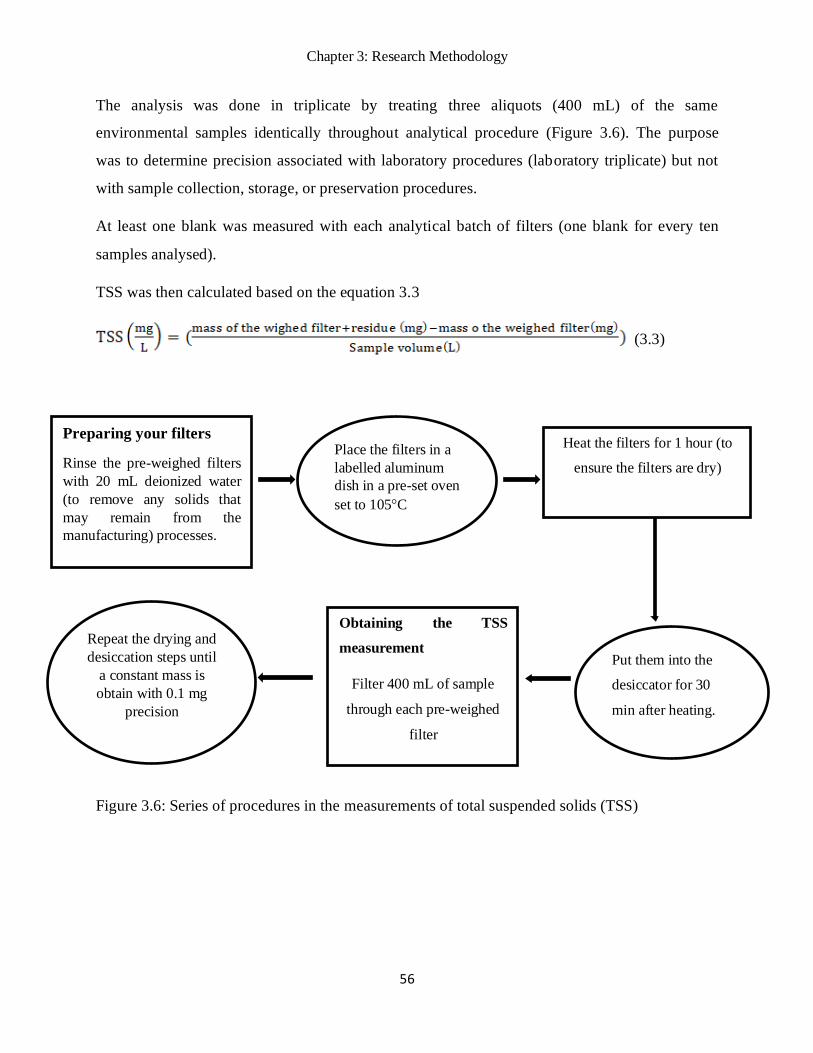
Chapter 3: Research Methodology
56
The analysis was done in triplicate by treating three aliquots (400 mL) of the same
environmental samples identically throughout analytical procedure (Figure 3.6). The purpose
was to determine precision associated with laboratory procedures (laboratory triplicate) but not
with sample collection, storage, or preservation procedures.
At least one blank was measured with each analytical batch of filters (one blank for every ten
samples analysed).
TSS was then calculated based on the equation 3.3
(3.3)
Figure 3.6: Series of procedures in the measurements of total suspended solids (TSS)
Preparing your filters
Rinse the pre-weighed filters
with 20 mL deionized water
(to remove any solids that
may remain from the
manufacturing) processes.
Place the filters in a
labelled aluminum
dish in a pre-set oven
set to 105C
Heat the filters for 1 hour (to
ensure the filters are dry)
Put them into the
desiccator for 30
min after heating.
Obtaining the TSS
measurement
Filter 400 mL of sample
through each pre-weighed
filter
Repeat the drying and
desiccation steps until
a constant mass is
obtain with 0.1 mg
precision

Chapter 3: Research Methodology
57
3.7 Total petroleum hydrocarbons (TPH)
Total petroleum hydrocarbons (TPH) is the term normally used to describe the number of
petroleum-based hydrocarbons extracted and quantified by a particular method in an
environmental sample matrix. The main constituents of TPHs include degraded crude oils,
combusted fossil fuels, and normal alkanes compounds that are less soluble in water but are
readily adsorbed onto particulate matter and are subsequently scavenged to the bottom sediment
which has become a reservoir for several hydrophobic contaminants.
It is one of the parameters that is included in the guidelines for oil-produced effluents and
therefore it is included in the parameters that form part of the model equation to predict the
compliance to guidelines of oil-produced effluents.
3.7.1 Sample preparation for extraction of petroleum compounds in oil-produced water
Liquid - liquid extraction (LLE) method was developed and applied for the extraction of TPHs
from OPW. Prior to LLE step, samples were filtered based on the (EPA method 3500C organic
extraction and sample preparation, 2007)(Figure 3.2). Extractions were performed within 14 days
after sampling. Extraction solvents that were used includes Ethyl acetate, Dichloromethane
(DCM), and n-hexane, (optimization for the best solvent was done using samples from the
depot). For further removal of moisture, the extracts were passed through sufficient anhydrous
sodium sulphate (Na2SO4) with glass wool at the bottom (Figures 3.7 & 3.8). The Na2SO4 was
purified by heating at 250°C overnight prior to the analysis.

Chapter 3: Research Methodology
58
Figure 3.7: Schematic diagram of removal of the moisture using Na2SO4 (Picture by LE
Monatisa, 2020).

Chapter 3: Research Methodology
59
Figure 3.8: An outline of the LLE procedure used to extract TPH from OPW samples.
Sample Preparation
500mL oily wastewater sample +
matrix spiking with 0.05 mg/L of
surrogate standard
Transfer the sample into a
separatory Funnel
Extraction
20mL of the extraction solvent added
into a separatory funnel and extracted
the sample three times
23232323
Combine the extracts
and evaporate to
dryness at 35 C under
nitrogen stream
Reconstitute the extract with 1 ml
solvent extract and stored at -18C prior
to analyses

Chapter 3: Research Methodology
60
3.7.2 Clean-up of LLE extracts using silica gel
The EPA clean up method (EPA METHOD 3630C, 1996) was followed for the clean-up of
OPW (LLE) extracts for TPH measurements. The extracts were cleaned up in a chromatographic
column packed with the slurry prepared from 10 g activated silica gel and 2 cm Na2SO4 layer on
top. This process was necessary in order to remove polar organic substances on the extracts prior
to the TPH determination (Daniel and Nna, 2016). The samples were then eluted using 20 mL of
n-pentane, concentrated and solvent exchanged to n-hexane. For quality assurance a blank
sample was processed the same way. A schematic diagram of the cleaning process is shown
Figure 3.9.

Chapter 3: Research Methodology
61
Figure 3.9: Schematic diagram of the silica gel clean-up (Picture by LE Monatisa, 2020).

Chapter 3: Research Methodology
62
3.7.3 Preparation of standard solutions for GC x GC-TOF MS
The primary standard stock solution was prepared by dissolving 123 μL of 99 % 1-
clorooctadecane in 877 μL ethyl acetate (LC-MS grade) in a 1.5 mL amber vial and then kept at
<4 ◦C till the time for analysis. The stock solution was then dissolved for 5 min under vortex
(David W. Burden, 2014). From the primary stock standard solution, working calibration
standard solutions of various concentrations were prepared in the range between 10 mg/L–100
mg/L for linearity, precision and recovery determinations.
3.7.4 Measurements of TPH using GC x GC-TOF-MS
Gas chromatography coupled with time of flight mass spectrometer (GCxGC-TOF-MS) was
used for the separation and detection of the TPH extracts (analytes). DCM, ethyl acetate and n-
hexane extracts of the TPHs were analysed by a LECO Pegasus 4D GCxGC-TOF-MS and
helium was used as carrier gas. The analysis of samples using GCxGC-TOF-MS was performed
within 40 days after the LLE extraction. The 1º GC column was Restek Rxi®-5Sil MS, 30m,
0.25mm ID, 0.25μm (Cochran, Pijpelink and Corporation, 2011). The analysis was done in a
split mode using temperature programming whereby for the 1º column the initial temperature is
40ºC holding for 1 minute then ramp to 320ºC at 1.3º/min and hold for 1 minute. The initial
temperature for the 2º column was 45ºC and the modulation offset temperature was 20ºC. The
modulation time was 3 sec while pulse time was 1 sec. The MS data collection was performed at
1 spectra/sec.
3.8 Model development
3.8.1 Establishing units of measurements in the model development
The standard units of evaporation measurements of both the OPWE and CWE were expressed in
mm/day. Evaporation rate was measured in terms of water level changes based on the differences
observed between two consecutive days and expressed in mm per day (mm/day). The
environmental parameters including TDS, TSS, TPH, TOC, COD and BOD were all expressed
in milligram per liter (mg/L). In addition, the unit for EC of both clear water and OPW was
expressed in micro Siemens per centimeter (μS/cm). The water temperature of both clear water
(Tcwe) and OPW (Topw) and air temperature (Ta) were measured in degrees Celsius (°C). Other

Chapter 3: Research Methodology
63
parameters such as wind speed (W) was expressed in meter per second (m/s) whereas solar
radiation (R) was measured in Lux but converted to Joules per unit time to relate the energy
balance of the system.
In modeling and generation of the real experimental data, the main objective was to reduce the
number of independent variables, to simplify the solution and to generalize the results thereof
(Ready, GM, 2014). Following the dimensional analysis based on the Buckingham theorem
(Buckingham, 1914), the parameters were expressed in terms of basic properties as shown in
Table 3.1 i.e. their dimensions (length, mass, time and temperature).
Table 3.1: Conversion of parameters to its dimensions.
Parameters SI units Dimensions
OPWE mm/day LT-1
CWE mm/day LT-1
R J/s MT-3
W m/s LT-1
Ta (°C) Θ
Tow (°C) Θ
EC μS/cm T-1
TOC mg/L ML-3
COD mg/L ML-3
BOD mg/L ML-3
TPH mg/L ML-3
TSS mg/L ML-3
TDS mg/L ML-3

Chapter 3: Research Methodology
64
3.9 OPWE Equation Derivation
The measured daily cumulative OPWE, daily cumulative CWE, OPW variables including TPH,
TOC, BOD, COD, EC, TDS, TSS, and TOPW and climatic variables including W, Ta and daily
cumulative solar radiation R were considered for this analysis. Dimensions of OPWE, CWE,
TPH, TOC, BOD, COD, EC, TDS, TSS, TOPW, W, Ta, and R respectively were L, L, ML-3,
ML-3, ML-3, ML-3, T-1, ML-3, ML-3, θ, LT-1, θ, and MT-2 (M: Mass, T: Time, L: Length, θ:
Degree). Therefore, the number of variables was 13 and the number of basic dimensions was 4,
meaning that all the variables can be combined into 9 (13 – 4) dimensionless variables ( terms)
to construct the final model.
Since the key role of the water body temperature in relation to air temperature in influencing the
trend of evaporation from water bodies (Izady et al. 2016), this work contemplated TOPW/Ta to
be one of the dimensionless variables. After an extensive search for the best model (Appendix 1),
OPWE, CWE, EC, TPH, TSS, TOC, BOD and COD were regarded as the best non-repeating
variables and hence TDS, W, and R were chosen as repeating variables, leading to the following
dimensionless variables:
(3.4)
where a1, a2, a3, a4, a5, a6, a7, a8, b1, b2, b3, b4, b5, b6, b7, b8, c1, c2, c3, c4, c5, c6, c7, and c8 are the
powers of each variable making the Π terms dimensionless and were solved by equating the units
as follows:

Chapter 3: Research Methodology
65
(3.5)
By solving Eq. (3.5) for the powers, the pi () terms were obtained as follows:
(3.6)
Considering the general form of Π terms function, Π1 = f (Π2, Π3, Π4, Π5, Π6, Π7, Π8, Π9 =
TOPW/Ta), Eq. (3.7) results in the general formulation for the OPW evaporation as follows:
(3.7)
A multiplicative form of the function f was applied, leading Eq. (3.8) to the final mathematical
model for the OPW evaporation:
(3.8)
where C, α, β, γ, , , , and (all dimensionless) are constants to fit the equation to the true
physical relationship holding in reality and were determined using a regression analysis on the
experimental data.

Chapter 3: Research Methodology
66
3.10 Statistical analysis
The statistical package for social sciences (IBM SPSS Statistics version 25 was used for data
analysis. The analysis of variance (ANOVA) was used to determine statistically significant
differences in the concentration of the OPW collected at an oil depot at a 0.05 confidence level
of significance using the Microsoft excel 2016.
3.11 Compliance study
Department of Water affairs and water research commission (DWAF and WRC, 1995),
Department of Water Affairs (DWAF) and Government Gazette, 1984 guidelines were used to
assess compliance of the OPW effluents due to the prevailing environmental conditions in SA
and the scope of parameters stated in the guidelines.

Chapter 3: Research Methodology
67
3.12 References
Adeniji, A. O., Okoh, O. O. and Okoh, A. I. (2017) ‘Petroleum Hydrocarbon Profiles of Water
and Sediment of Algoa Bay , Eastern Cape , South Africa’, International Journal of
Environmental Research and public Health, 10(14), pp. 1–21. doi: 10.3390/ijerph14101263.
Akporido, S. O. and Onianwa, P. C. (2015). ‘Heavy Metals and Total Petroleum Hydrocarbon
Concentrations in Surface Water of Esi River, Western Niger Delta’. Research Journal of
Environmental Sciences, 9: 88-100.
Buckingham, E. (1914) ‘On physically similar systems; Illustrations of the use of dimensional
equations’, Physical Review, 4(4), pp. 345–376. doi: 10.1103/PhysRev.4.345.
Cochran, J., Pijpelink, J. and Corporation, R. (2011) GCxGC Analysis of Complex Petroleum
Hydrocarbons : Sulphur Speciation in Diesel.
Daniel, I. E. and Nna, P. J. (2016) ‘Total Petroleum Hydrocarbon Concentration in Surface
Water of Cross River Estuary, Niger Delta, Nigeria’, Asian Journal of Environment & Ecology,
1(2), pp. 1–7. doi: 10.9734/ajee/2016/31102.
Department of Water Affairs. (2013) Revision of general authorisations in terms of Section 39 of
the National Water Act, 1998 (Act No. 36 of 1998), No. 665. Government Gazette No. 36820, 6
September. Department of Water Affairs, Pretoria, South Africa.
EPA METHOD 3500C ORGANIC EXTRACTION AND SAMPLE PREPARATION (2007)
3500C - 1 Revision 3 February 2007.
EPA METHOD 3630C (1996) SILICA GEL CLEANUP.
Government Gazette (1984) Requirements for the Purification of Wastewater or Effluent.
Gazette No 9225, Regulation No 991, 18 May.
Izady A., Abdalla, O., Sadeghi, M., Majidi, M,. Karimi, A., and Chen M., (2016). Novel
Approach to Modeling Wastewater Evaporation Based on Dimensional Analysis, Water
Resources Management. Water Resources Management, 30, pp. 2801–2814. doi:
10.1007/s11269-016-1324-8.
ToxFAQs, A. for T. S. and D. R. (1999) Total Petroleum Hydrocarbons (Tph) Agency For Toxic
Substances And Disease Registry Toxfaqs. Available at:
http://www.atsdr.cdc.gov/toxfaq.html%0Ahttps://www.atsdr.cdc.gov/toxfaqs/tfacts123.pdf.

68
CHAPTER 4 : IDENTIFICATION OF TOTAL PETROLEUM
HYDROCARBONS IN OIL PRODUCED WATER
This chapter discusses the results and observations for experiments done on the analysis of TPH
in OPW samples. The TPH analysis and identification results are presented mainly qualitative
with the exception of 1-chloro-octadecane, the surrogate standard. The results and discussion on
the TPH compounds that were identified based on similarity index to the databases are presented
and discussed in this chapter.
4.1 Introduction
In this chapter, an analytical method based on liquid-liquid extraction (LLE) and gas
chromatography coupled to time of flight-mass spectrometry GC-TOF-MS was developed for
the determination of total petroleum hydrocarbon (TPHs) in oil produced water (OPW) from an
oil refinery plant. The extraction of the TPHs was achieved based on LLE technique using
various extraction solvents. After the extraction the GC-MS was used to separate and identify the
TPHs compounds. The extraction method involved mainly LLE after optimization of several
controlling parameters followed by a cleanup process using column packed with silica gel. The
GC-TOF-MS run of the extracts was then conducted. The details of the experimental procedures
that were followed for TPH analysis is provided in Chapter 3 of this dissertation.
Normally contamination due to petroleum products in the environment can be identified and
ascertained by determining TPHs which provides minimum information regarding the petroleum
hydrocarbon present in the sample. However, certain compounds within the TPHs if present in
water or edible products are known to be capable of inducing negative effects on human health
(Alegbeleye, et al., 2017).
Chapter 4: Identification of Total Petroleum Hydrocarbons in Oil Produced Water
69
4.2 The development and optimization of the separation and detection method for TPHs
using GC-TOF-MS
Prior to the actual extraction of analytes from environmental samples, it is desired that, the
separation and detection method be developed and optimized. The choice of GC-TOF-MS as a
separation and detection method, stemmed from the observation of the chemistry of the analytes
which are known to be volatile and of low molecular weight. Gas chromatography (GC) is
suitable for such compounds and hence the reason for the choice.
The stationary phase (GC column) used and MS conditions used are described in Chapter 3
section 3.7.
Method development used the surrogate standard (1-chloro-octadecane) which was dissolved in
the appropriate solvent and injected onto the GC-TOF-MS. The signal (chromatographic peak)
was observed at around 18 minutes retention time. The MS fragmentation pattern confirmed the
identification of this compound.
Figure 4.1 shows the chromatograms obtained from the GC-TOF-MS run of the 1-chloro-
octadecane.

Chapter 4: Identification of Total Petroleum Hydrocarbons in Oil Produced Water
70
6:40.00 10:00.00 13:20.00 16:40.00 20:00.00 23:20.00 26:40.00
2000
3000
4000
5000
6000
7000
8000
9000
Time (min:sec)
Oct
adeca
ne,
1-c
hlo
ro-
57
Figure 4.1a GC-MS chromatogram of standard sample, 1-chloro-octadecane
Figure 4.1a, shows the mass chromatogram of surrogate standard, 1-chloro-octadecane appeared
at ~18minutes. This showed the success of the method developed and therefore it provided the
means to identify the compound from OPW samples and which made the quatitation and
qualitation of the compound possible. The identification of 1-chloro-octadecase was further
confirmed by the mass spectral data (Figure 4.1b) where the fragmentation pattern aligned well
with MS spectral pattern of the cmpound as also verified by the NIST-Library.

Chapter 4: Identification of Total Petroleum Hydrocarbons in Oil Produced Water
71
20 40 60 80 100 120 140 160 180 200 220 240 260 280 300 320 340 360 380 400 420 440 460 480 500 520 540 560 580 600
200
400
600
800
1000 43 57
69 91 27
105 278 232 506 438 334 133 534 552 316 414 375 210 458 259 584 359 185
Peak True - sample "Inffluent 2" (25/11/2019):1", peak 5, at 18:27.40 min:sec
20 40 60 80 100 120 140 160 180 200 220 240 260 280 300 320 340 360 380 400 420 440 460 480 500 520 540 560 580 600
-500
0
500
1000
41
55 27 278 506 438 334 527 316 232 414 552 458 210 64 375 584 251 359 186
288 217 189 161 58 29 42 111 97 85
71
Peak True - sample "Inffluent 2" (25/11/2019):1", peak 5, at 18:27.40 min:sec vs. Library Hit - similarity 855, "Octadecane, 1-chloro-"
20 40 60 80 100 120 140 160 180 200 220 240 260 280 300 320 340 360 380 400 420 440 460 480 500 520 540 560 580 600
200
400
600
800
1000 57
71 43
85
29 133 161 189 288 217 245
Library Hit - similarity 855, "Octadecane, 1-chloro-"
Figure 4.1b Mass spectral pattern of standard (1-chloro-octadecane)
4.3 Liquid – Liquid Extraction (LLE) of TPHs from OPW
In this study, LLE was selected as sample preparation method of choice for TPHs over others
reported in literature simply because it is among the validated methods by EPA for TPH
extraction from matrices similar to what this study dealt with.
Several organic solvents were identified and optimized for their efficiency potential to extract
TPHs in OPW samples. These solvents included, n-hexane, ethyl acetate and dichloromethane
(DCM). (Figure 4.2).

Chapter 4: Identification of Total Petroleum Hydrocarbons in Oil Produced Water
72
0
20
40
60
80
100
DCM Ethyl Acetate n-Hexane
77.16 79.39
96.28
Rec
ove
ries
(%)
Solvents
Figure 4.2: Optimization of the extraction solvents for TPH
4.3.1 Effect of the organic phase on the extraction efficiency
The optimization results for the organic solvents most suitable in the extraction of TPHs from
OPW are presented in Figure 4.2 which clearly shows that n-hexane gave a better performance.
This may be attributed to the polarity of the solvent. Of the solvent tested, n-hexane is the most
non-polar and thus dissolved the compound better than other solvents. Therefore n-hexane was
used in all subsequent extraction experiments for TPH from OPW samples.
4.3.2 Optimization of organic solvent and the determination of extraction recovery
efficiency
The organic solvents that were selected and optimized included dichloromethane (DCM), ethyl
acetate and n-hexane. These solvents were selected because they have low miscibility with
water, and high solubility for the target analytes. The spiked deionized water was used to
investigate the recovery efficiency whereby 1-chlorooctadecane was used as a surrogate
indicator. The surrogate indicator was spiked into 500 mL of denoised water before extraction
and concentration step. Then the spiked water was added into the separatory funnel using a
measuring cylinder followed by the 20 mL of the organic sample.
The efficiency of LLE of the analytes was obtained using equation 4.1:

Chapter 4: Identification of Total Petroleum Hydrocarbons in Oil Produced Water
73
(4.1)
Where C1, C2 and C3 are the mean concentration of the analytes obtained. The relative standard
deviation was calculated to obtain the precise extraction recovery. For quality insurance
purposes, the blanks were prepared same way as the synthetic samples but without the inclusion
of the surrogate standard.
The details of the experimental protocols have been given in Chapter 3 of this dissertation.
Generally, the recoveries of 1-chlorooctadecane spiked in water samples were between 77% and
96%, which is within the acceptable range of 40–140% for hydrocarbons (Adeniji, Okoh and
Okoh, 2017; Kansas Department of Health and Environmental, 2015). The recoveries recorded
were 96.28% for n-hexane; 77.39% for ethyl acetate and 77.16 for DCM (Figure 4.2). Therefore,
n-hexane as an extracting solvent presented higher recovery as compared to other solvents. This
may be attributed to its greater non-polar nature, low latent heat of vaporization (330 kJ/kg) and
high selectivity to analytes as compared to other solvents (Lee, S., 2015). This is in agreement
with many other researchers who have also reported on n-Hexane as being the best extract
solvent particularly for TPH.
4.4 Calibration experiments
The quantification of the analyte in this study was performed using the external calibration
curve. Linearity was demonstrated using the coefficient of liners regression (r2) and was higher
than 0.99 (Figure 4.3). The r2 value obtained is acceptable and showed that the calibration curve
can reliably be used for the quantification purposes (Agency for Toxic Substances Disease
Registry, 1999). The calibration curve obtained from a plot of peak areas against concentrations
of 1-chlorooctadecane that were run in the GC-TOF-MS. The 1-chlorooctadecane was found to
exhibit a linear relationship for concentrations from 10mg/L to 100mg/L. This linear range is
suitable as it assures that even if the concentration from the real sample is high or low, the same
calibration curve will be suitable to identify and quantify the target compounds.

Chapter 4: Identification of Total Petroleum Hydrocarbons in Oil Produced Water
74
20 40 60 80 100 120 140
1000000
2000000
3000000
4000000
5000000
6000000
7000000
8000000
9000000
Concentration
Are
a
10 ppm:1
40 ppm :1
60 ppm:2
80 ppm:1
90 ppm:1
100 ppm:2
y= +90488.2x - 819110r = 0.99171
Figure 4.3: Calibration curve for 1-chlorooctadecane as a surrogate standard for THPs .
4.5 Limit of detection and quantification determination using GC-MS.
The limit of detection (LOD) and limit of quantification (LOQ) for TPH were estimated from
the calibration curve. The working standards used for the preparation of the calibration curve
were prepared from the pure analytical chemicals and they ranged from 10 mg/L to 100 mg/L.
The LOD and LOQ were determined based on the signal-to noise ratio (S/N) of 3 and 10X
respectivewly based on the residual standard deviation (SD) of the y-intercept of the regression
line of the calibration curve and sensitivity of slope of the regression line (equations 4.2 and 4.3):
(4.2)
(4.3)
To confirm the accuracy, both the LOD and LOQ were analyzed in triplicate to detect the TPHs
at varying concentrations.
The LOD and LOQ of TPH using 1-chlorooactadecane surrogate standard were 100 and 355
ng/L respectively and they were obtained using GC-MS.

Chapter 4: Identification of Total Petroleum Hydrocarbons in Oil Produced Water
75
4.6 Quality Control
To ensure that the TPH measurements were a true representative of the oilfield matrix, quality
control procedures to address issues including contamination, accuracy and precision of the
results were conducted. All reagents and solvents used were of analytical and LCMS grades.
Samples were analyzed in triplicates with blanks and spiked samples. The precision was
estimated as the relative standard deviation (RSD) varied from 6.57 to 10.21% were found to be
less than the maximum limit of 25% (Kansas Department of Health and Environmental, 2015;
Texas Natural Resource Conservation Commission, 2001)
4.7 Analysis of TPHs in samples collected from petroleum industry.
After the sample preparation step, the extract was evaluated and analysed for TPHs. Various
fractions were analysed including, n-alkanes, branched alkanes, alkenes, etc. by gas
chromatography analysis GC-TOF-MS. The TPH compounds were characterized based on
similarities between their mass spectrum and t NIST Library.
4.7.1 Measurements of TPHs in oil produced water
The oil produced water (OPW) from the wastewater treatment plant at an oil refinery was
collected for the determination of TPH. Three samples from the influent and three from the
effluent compartments were collected. After sample preparation procedures, the GC-MS was
used for the determination of TPH. Samples for TPH analysis were collected weekly from May
to December 2010 in a period that covered winter, autumn, spring, and summer. The study aimed
at investigating the seasonal variation of TPH at the depot.
4.7.2 GC-MS analysis of blank samples
The analysis of the blank sample showed no presence of TPH compounds but rather other non-
TPH compounds (Figures 4.4a and 4.4b).

Chapter 4: Identification of Total Petroleum Hydrocarbons in Oil Produced Water
76
6:40.00 10:00.00 13:20.00 16:40.00 20:00.00 23:20.00 26:40.00
50000
100000
150000
200000
250000
300000
350000
400000
450000
Time (min:sec)
Oct
adeca
ne,
1-c
hlo
ro-
57
Figure 4.4a GC-MS chromatograms of the blank sample
20 40 60 80 100 120 140 160 180 200 220 240 260 280 300 320 340 360 380 400 420 440 460 480 500 520 540 560 580 600
200
400
600
800
1000 41
57
71 91 29
83
147 175
Peak True - sample "Effluent 3' (06/12/2019):1", peak 20, at 18:17.30 min:sec
20 40 60 80 100 120 140 160 180 200 220 240 260 280 300 320 340 360 380 400 420 440 460 480 500 520 540 560 580 600
-500
0
500
1000 41
55 29
91 69 111
189 169 288 135 113 99 57 85 71
Peak True - sample "Effluent 3' (06/12/2019):1", peak 20, at 18:17.30 min:sec vs. Library Hit - similarity 855, "Octadecane, 1-chloro-"
20 40 60 80 100 120 140 160 180 200 220 240 260 280 300 320 340 360 380 400 420 440 460 480 500 520 540 560 580 600
200
400
600
800
1000 57
71 43
85
29 133 161 189 288 217 245
Library Hit - similarity 855, "Octadecane, 1-chloro-"
Figure 4.4b Shows the mass spectral pattern of the blank sample

Chapter 4: Identification of Total Petroleum Hydrocarbons in Oil Produced Water
77
4.7.3 Alkane hydrocarbons in the influent samples in autumn 2019
The influent samples showed the presence of different classes of TPHs including alkanes,
alkenes, branched chain alkanes, branched alkenes, alkynes, cyclic aromatic hydrocarbons (Table
4.1).
Table 4.1a shows the profile of n-alkanes found in the oil produced water samples. The results
showed that the influent contained more n-alkanes than the effluent. A total of 12 compounds
were identified from the influent samples versus 9 that were found in the effluent samples. n-
alkane hydrocarbons in the influent samples had carbon chain lengths between C 11 to C40 and
of these there was a 50:50 ratio between those which are even numbered to those which are odd
numbers. Compounds with carbon chain length more than 21 were more than those with less 21.
The relative higher abundance of higher molecular weight alkanes signals to petroleum
hydrocarbons in the matrix while the lower alkanes signals to the freshness of hydrocarbons in
the environment (Tornero and d'Alcalà, 2014)
In the effluent samples, 9 compounds were identified with carbon chain lengths ranging from
C14 to C36. The ratio of the even numbered alkanes to odd numbered alkanes was 55:45. The
ratio of higher to lower hydrocarbons was found to be 55:45.
The measure of evenness or oddness of the alkanes provide an indication of the source of these
compounds in the environment. Generally, the even numbered alkanes give an indication of the
anthropogenic input while the odd numbered hydrocarbons provide an indication of the natural
source of the compounds (Kachel,2008)

Chapter 4: Identification of Total Petroleum Hydrocarbons in Oil Produced Water
78
Table 4.1a straight chain-alkane hydrocarbons (n-alkanes) in oil produced water from an
oil refinery plant for samples collected in autumn 2019
Autumn n-alkane hydrocarbons profile
Influent Effluent
Name Formula Name Formula
Dodecane C12H26 Hexatriacontane C36H74
Heneicosane C21H44 Hexadecane C16H34
Hentriacontane C31H64 Nonadecane C19H40
Heptacosane C27H56 Octacosane C28H58
Heptadecane C17H36 Heptadecane C17H36
Hexadecane C16H34 Tetradecane C14H30
Hexatriacontane C36H74 Octacosane C28H58
Nonadecane C19H40 Heneicosane C21H44
Octacosane C28H58 Heptacosane C27H56
Tetracontane C40H82
Tetracosane C24H50
Undecane C11H24
Table 4.1b depicts the profile of branched chain alkanes which were the dominant group of
alkanes that were found in the OPW samples. A total of 24 compounds were identified from the
influent samples and 16 compounds in effluent samples. The higher abundance of branched
chain alkanes in the OPW can be as a result of the chemical and microbial actions that occurs
while the treatment process is going on.
The observation that, effluent samples contained fewer compounds than the influent can be
explained by the fact that the treatment process does remove them as well as the fact that, some
may become complexed with the solid matter at the bottom.

79
Table 4.1b branched chain-alkane hydrocarbons in oil produced water from an oil refinery plant for samples collected in autumn 2019
Autumn TPH profile of branched chain alkane hydrocarbons
Influent Effluent
Name Formula Name Formula
1-Nonylcycloheptane C16H32 Dodecane, 2,6,10-trimethyl- C15H32
Benzene, [3-(2-cyclohexylethyl)-6-cyclopentylhexyl]- C25H40 Undecane, 3,9-dimethyl- C13H28
Bicyclo [3.1.0] hexan-2-one, 5-(1-methylethyl)- C9H14O Tetradecane, 2,6,10-trimethyl- C17H36
Decane, 2,3,5,8-tetramethyl- C14H30 Dodecane, 2,6,10-trimethyl- C15H32
Decane, 3,7-dimethyl- C12H26 1-Nonylcycloheptane C16H32
Dodecane, 1-fluoro- C12H25F 1-Pentene, 3-ethyl-2-methyl- C8H16
Dodecane, 2,6,10-trimethyl- C15H32 1,4-Hexadiene, 2,3,4,5-tetramethyl- C10H18
Heptadecane, 2,6,10,14-tetramethyl- C21H44 Pentadecane, 2,6,10-trimethyl- C18H38
Heptyl triacontyl ether C37H76O 4-Undecene, 10-methyl-, (E)- C12H24
Hexanal, 4,4-dimethyl- C8H16O Undecane, 2-cyclohexyl- C17H34
Hexane, 3,3,4,4-tetramethyl- C10H22 Hexane, 3,3-dimethyl- C8H18
Nonadecane, 2-methyl- C20H42 Dodecane, 2,6,10-trimethyl- C15H32
Nonane, 2,2,4,4,6,8,8-heptamethyl- C16H34 Undecane, 2,10-dimethyl- C13H28
Nonane, 5-methyl- C10H22 2-Undecene, 7-methyl- C12H24
Octadecane, 3-ethyl-5-(2-ethylbutyl)- C26H54 Octane, 4-methyl- C9H20
Octane, 2,6-dimethyl- C10H22 Heptadecane, 2,6,10,14-tetramethyl- C21H44
Octane, 4-methyl- C9H20
Oxetane, 3,3-dimethyl- C5H10O
Tetradecane, 2,6,10-trimethyl- C17H36
Tridecane, 6-methyl- C14H30
Tridecane, 7-cyclohexyl- C19H38
Undecane, 2,2-dimethyl- C13H28
Undecane, 3,5-dimethyl- C13H28
Undecane, 3,6-dimethyl- C13H28

80
Table 4.1c shows the profile of alkene hydrocarbons that were found in the OPW samples. The
result shows that, alkene hydrocarbons were few as compared to the straight chain and branched
chain alkanes. Seven (7) alkene hydrocarbon compounds were detected in the influent samples
and only two (2) in the effluent samples. This can be attributed to the fact that, some chemical
reactions such as photochemical reactions, action of microorganisms might be responsible for
hydrogenation of enzymatic reduction of the double bonds thus making saturated compounds
lose their unsaturation which resulted into fewer alkene hydrocarbons in the samples.
Table 4.1c: Alkene hydrocarbons in oil produced water from an oil refinery plant for samples
collected in autumn 2019
Autumn TPH profile of alkene hydrocarbons
Influent Effluent
Name Formula Name Formula
1,12-Tridecadiene C13H24 Nonacos-1-ene C29H58
17-Pentatriacontene C35H70 17-
Pentatriacontene C35H70
3-Tetradecene, (E)- C14H28 Heptacos-1-ene C27H54
4-Methyl-1,3-heptadiene C8H14
4-Nonene, 2,3,3-trimethyl-, (Z)- C12H24
Cyclohexane, [6-cyclopentyl-3-
(3-cyclopentylpropyl) hexyl]- C25H46
Nonacos-1-ene C29H58
Cyclic alkanes were also found to be present in the oil produced samples. Table 4.1d shows the
profile of these compounds with a similar pattern as already discussed for alkanes and alkenes
where the influent samples contained more of these compounds (in terms of number of
compounds) than the effluent. This can as well be attributed to the efficiency of the treatment
process.

Chapter 4: Identification of Total Petroleum Hydrocarbons in Oil Produced Water
81
Table 4.1d: cyclic-alkane hydrocarbons in oil produced water from an oil refinery plant for
samples collected in autumn 2019
Autumn TPH profile of cyclic hydrocarbons
Influent Effluent
Name Formula Name Formula
1-Nonylcycloheptane C16H32 Cyclopentane,
methyl-
C6H12
Cyclobutane, ethyl- C6H12 Cyclooctane,
butyl- C12H24
Cyclohexane, [6-cyclopentyl-3-
(3-cyclopentylpropyl) hexyl]- C25H46
Cyclobutane,
ethyl-
C5H12
Cyclohexane, [6-cyclopentyl-3-
(3-cyclopentylpropyl) hexyl]- C25H46
Cyclopropane, 1-
ethyl-2-heptyl- C12H24
Cyclohexane, 1,1,3,5-
tetramethyl-, cis- C10H20
Cyclopentane,
methyl- C6H12
Cyclohexane, 1,3,5-trimethyl-2-
octadecyl- C27H54
Cyclooctane, 1,4-dimethyl-, cis- C10H20
Cyclotetradecane C14H28
The results also showed the presence of few alkyne hydrocarbons as Table 4.1depicts. In this
table, it shows that some compounds, mainly 3-Octyne, 7-methyl-, appear in both the influent as
well as the effluent. This can be an indication of incomplete treatment of such compounds.
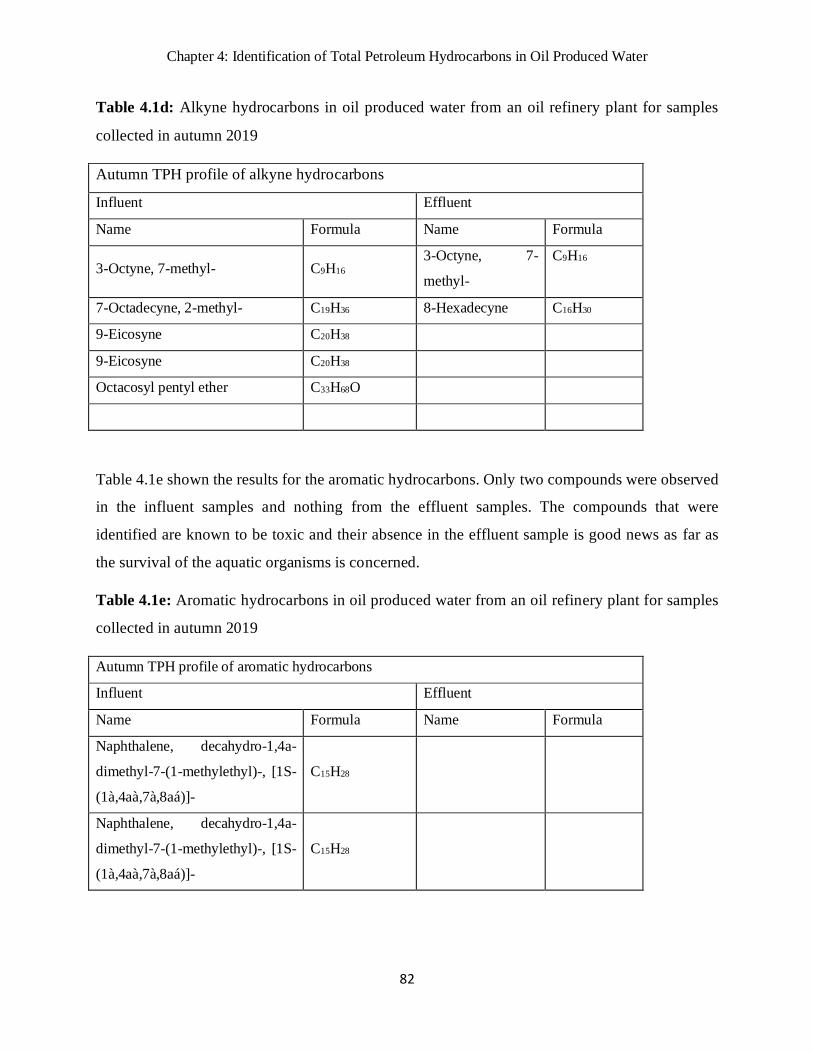
Chapter 4: Identification of Total Petroleum Hydrocarbons in Oil Produced Water
82
Table 4.1d: Alkyne hydrocarbons in oil produced water from an oil refinery plant for samples
collected in autumn 2019
Autumn TPH profile of alkyne hydrocarbons
Influent Effluent
Name Formula Name Formula
3-Octyne, 7-methyl- C9H16 3-Octyne, 7-
methyl-
C9H16
7-Octadecyne, 2-methyl- C19H36 8-Hexadecyne C16H30
9-Eicosyne C20H38
9-Eicosyne C20H38
Octacosyl pentyl ether C33H68O
Table 4.1e shown the results for the aromatic hydrocarbons. Only two compounds were observed
in the influent samples and nothing from the effluent samples. The compounds that were
identified are known to be toxic and their absence in the effluent sample is good news as far as
the survival of the aquatic organisms is concerned.
Table 4.1e: Aromatic hydrocarbons in oil produced water from an oil refinery plant for samples
collected in autumn 2019
Autumn TPH profile of aromatic hydrocarbons
Influent Effluent
Name Formula Name Formula
Naphthalene, decahydro-1,4a-
dimethyl-7-(1-methylethyl)-, [1S-
(1à,4aà,7à,8aá)]-
C15H28
Naphthalene, decahydro-1,4a-
dimethyl-7-(1-methylethyl)-, [1S-
(1à,4aà,7à,8aá)]-
C15H28

Chapter 4: Identification of Total Petroleum Hydrocarbons in Oil Produced Water
83
4.8 Winter profile of TPHs in oil produced water samples from an oil petroleum industry
The winter period (June-August) registered many compounds especially from the influent
compartments than they were found in Autumn season. Table 4.2a shows a comparison for the
influent profile of hydrocarbons.
From Table 4.2, it is evident that branched chain alkanes dominated the profile of hydrocarbons
that were found in the samples for wither season. The ratio of branched chain alkanes to n-
alkanes was found to be approximately 70:30. The aromatic hydrocarbons were not found and
only a few alkenes and alkynes hydrocarbons.
The effluent contained very few TPH compounds. This may mean that the quality of effluent
discharged from the plant in winter times is much better than other seasons
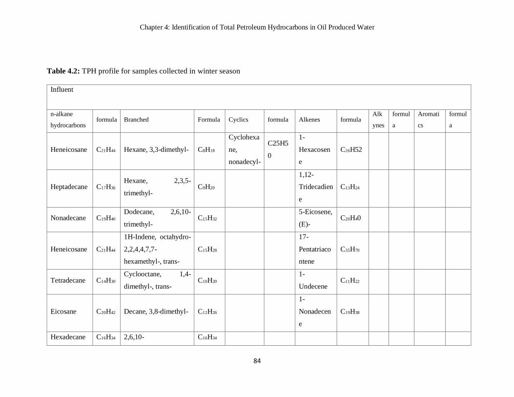
Chapter 4: Identification of Total Petroleum Hydrocarbons in Oil Produced Water
84
Table 4.2: TPH profile for samples collected in winter season
Influent
n-alkane
hydrocarbons formula Branched Formula Cyclics formula Alkenes formula
Alk
ynes
formul
a
Aromati
cs
formul
a
Heneicosane C21H44 Hexane, 3,3-dimethyl- C8H18
Cyclohexa
ne,
nonadecyl-
C25H5
0
1-
Hexacosen
e
C26H52
Heptadecane C17H36 Hexane, 2,3,5-
trimethyl- C9H20
1,12-
Tridecadien
e
C13H24
Nonadecane C19H40 Dodecane, 2,6,10-
trimethyl- C15H32
5-Eicosene,
(E)- C20H40
Heneicosane C21H44
1H-Indene, octahydro-
2,2,4,4,7,7-
hexamethyl-, trans-
C15H28
17-
Pentatriaco
ntene
C35H70
Tetradecane C14H30 Cyclooctane, 1,4-
dimethyl-, trans- C10H20
1-
Undecene C11H22
Eicosane C20H42 Decane, 3,8-dimethyl- C12H26
1-
Nonadecen
e
C19H38
Hexadecane C16H34 2,6,10- C16H34

Chapter 4: Identification of Total Petroleum Hydrocarbons in Oil Produced Water
85
Trimethyltridecane
Heptadecane C17H36 1,5-Hexadiene, 2,5-
dipropyl- C12H22
Heptadecane C17H36 Decane, 2,9-dimethyl- C12H26
Heptacosane C27H56 trans-Calamenene C15H22
Eicosane C20H42 Undecane, 4,7-
dimethyl- C13H28
Heneicosane C21H44 1-Decanol, 2-hexyl- C16H34
O
Heptadecane C17H36 Pentadecane, 2,6,10-
trimethyl- C18H38
Heneicosane C21H44 Cyclohexane, 1,3,5-
trimethyl-2-octadecyl- C27H54
Hexatriacont
ane C36H74
Tetradecane, 2,6,10-
trimethyl- C17H36
Heptacosane C27H56 Heptacosane, 1-chloro- C27H55C
l
Decane,
2,3,6-
trimethyl-
C13H28 Dodecane, 2,6,10-
trimethyl- C15H32
Heptacosane C27H56 1,12-Tridecadiene C13H24
Octacosane C28H58 Octadecane, 3-ethyl-5-
(2-ethylbutyl)- C26H54

Chapter 4: Identification of Total Petroleum Hydrocarbons in Oil Produced Water
86
Heptadecane C17H36 Octadecane, 3-ethyl-5-
(2-ethylbutyl)- C26H54
Heptacosane C27H56 Dodecane, 2,6,10-
trimethyl- C15H32
Pentadecane C15H32 Heptadecane C17H36
Heptadecane C17H36 Cyclohexane, 1,3,5-
trimethyl-2-octadecyl- C27H54
Heptacosane C27H56 cis-2-Methyl-7-
octadecene C19H38
Hentriaconta
ne C31H64
Butane, 2,3-dimethyl-
2-nitro-
C6H13N
O2
Heptacosane C27H56 Pentane, 2,3-dimethyl- C7H16
Hexadecane C16H34 Decane, 4-ethyl- C12H26
Pentadecane C15H32 Nonane, 3,7-dimethyl- C11H24
Hexatriacont
ane C36H74
Decane, 2,3,6-
trimethyl- C13H28
Hexadecane C16H34 Decane, 5-propyl- C13H28
Nonadecane C19H40 Undecane, 3-methyl- C12H26
Pentadecane C15H32 Tetradecane, 2,5-
dimethyl- C16H34
Hexadecane C16H34 Undecane, 4-ethyl- C13H28
Heneicosane C21H44 Decane, 2,3,5,8-
tetramethyl- C14H30

Chapter 4: Identification of Total Petroleum Hydrocarbons in Oil Produced Water
87
Hentriaconta
ne C31H64 Tridecane, 4-methyl- C14H30
Octadecane C18H38 Hexane, 3,3-dimethyl- C8H18
Hentriaconta
ne C31H64
Cyclopentane, 1-butyl-
2-propyl- C12H24
Heptadecane C17H36 Cyclohexane, (2-ethyl-
1-methylbutylidene)- C13H24
Heptadecane C17H36 Undecane, 4,6-
dimethyl- C13H28
Heptacosane C27H56 Octane, 3,5-dimethyl- C10H22
Eicosane C20H42 Decane, 2-methyl- C11H24
Pentadecane C15H32 2,2,7,7-
Tetramethyloctane C12H26
Heptacosane C27H56 Dodecane, 2,6,10-
trimethyl- C15H32
Hexatriacont
ane C36H74
Octane, 2,4,6-
trimethyl- C11H24
Heptacosane C27H56 Decane, 2,3,5,8-
tetramethyl- C14H30
Octacosane C28H58 Undecane, 5-ethyl- C13H28
Undecane C11H24 Dodecane, 2,6,10-
trimethyl- C15H32
Tetradecane C14H30 10-Methylnonadecane C20H42

Chapter 4: Identification of Total Petroleum Hydrocarbons in Oil Produced Water
88
Tridecane C13H28 Octadecane, 6-methyl- C19H40
Decane C10H22 Nonadecane, 9-
methyl- C20H42
Tetradecane C14H30 Methane,
tricyclohexyl- C19H34
Nonadecane C19H40 Decane, 2-methyl- C11H24
Tetradecane C14H
30
Dodecane, 2,6,10-
trimethyl- C15H32
Pentadecane C15H
32
Hexadecane,
2,6,10,14-tetramethyl- C20H42
Hexadecane C16H34 2-Methyltetracosane C25H52
Pentadecane C15H32 Decane, 2,5-dimethyl- C12H26
Heptadecane C17H36
Hexadecane C16H34 Dodecane, 2,6,10-
trimethyl- C15H32
Hexatriacont
ane C36H74
10-Methyl-9-
nonadecene C20H40
Tetradecane C14H30 2-Methyltetracosane C25H52
Nonadecane C19H40 Heptadecane, 2,3-
dimethyl- C19H40
Heptadecane C17H36 2-Methyltetracosane C25H52
Heptadecane C17H36 Decane, 4-methyl- C11H24
Eicosane C20H42 2,3-Dimethyldecane C12H26
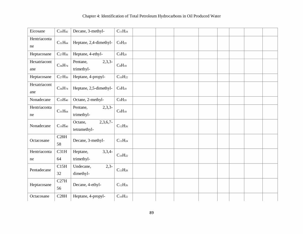
Chapter 4: Identification of Total Petroleum Hydrocarbons in Oil Produced Water
89
Eicosane C20H42 Decane, 3-methyl- C11H24
Hentriaconta
ne C31H64 Heptane, 2,4-dimethyl- C9H20
Heptacosane C27H56 Heptane, 4-ethyl- C9H20
Hexatriacont
ane C36H74
Pentane, 2,3,3-
trimethyl- C8H18
Heptacosane C27H56 Heptane, 4-propyl- C10H22
Hexatriacont
ane C36H74 Heptane, 2,5-dimethyl- C9H20
Nonadecane C19H40 Octane, 2-methyl- C9H20
Hentriaconta
ne C31H64
Pentane, 2,3,3-
trimethyl- C8H18
Nonadecane C19H40 Octane, 2,3,6,7-
tetramethyl- C12H26
Octacosane C28H
58 Decane, 3-methyl- C11H24
Hentriaconta
ne
C31H
64
Heptane, 3,3,4-
trimethyl- C10H22
Pentadecane C15H
32
Undecane, 2,3-
dimethyl- C13H28
Heptacosane C27H
56 Decane, 4-ethyl- C12H26
Octacosane C28H Heptane, 4-propyl- C10H22

Chapter 4: Identification of Total Petroleum Hydrocarbons in Oil Produced Water
90
58
Nonadecane C19H
40 Hexane, 2,4-dimethyl- C8H18
Heptacosane C27H56 Undecane, 4-methyl- C12H26
Hexatriacont
ane C36H74 Undecane, 2-methyl- C12H26
Dodecane, 4-methyl- C13H28
Undecane, 3-methyl- C12H26
Decane, 2,5-dimethyl- C12H26
Undecane, 2-methyl- C12H26
Decane, 2,3,7-
trimethyl- C13H28
Octadecane, 6-methyl- C19H40
Undecane, 5-ethyl- C13H28
Tridecane, 4-methyl- C14H30
Decane, 4-methyl- C11H24
Decane, 2,3,5,8-
tetramethyl- C14H30
Pentane, 2,2-dimethyl- C7H16
Undecane, 2,6-
dimethyl- C13H28
Decane, 4-ethyl- C12H26
Undecane, 3-methyl- C12H26

Chapter 4: Identification of Total Petroleum Hydrocarbons in Oil Produced Water
91
Undecane, 3,8-
dimethyl- C13H28
Dodecane, 3-methyl- C13H28
Undecane, 6-ethyl- C13H28
Octane, 2,3,7-
trimethyl- C11H24
10-Methylnonadecane C20H42
Undecane, 3,9-
dimethyl- C13H28
1,1,6,6-
Tetramethylspiro[4.4]n
onane
C13H24
Undecane, 4-ethyl- C13H28
Undecane, 2,6-
dimethyl- C13H28
Dodecane, 5-methyl- C13H28
1-Iodo-2-
methylnonane C10H21I
Tridecane, 4-methyl- C14H30
Decane, 2-methyl- C11H24
Nonane, 3-methyl- C10H22
Hexane, 3-ethyl-3-
methyl- C9H20

Chapter 4: Identification of Total Petroleum Hydrocarbons in Oil Produced Water
92
6-Tridecene, 7-methyl- C14H28
Hexane, 3-ethyl-3-
methyl- C9H20
Tridecane, 6-methyl- C14H30
Pentadecane, 7-
methyl- C16H34
Decane, 3,8-dimethyl- C12H26
Tetradecane, 6,9-
dimethyl- C16H34
Tetradecane, 4-methyl- C15H3
2
1-Iodo-2-
methylundecane C12H25I
Dodecane, 2-methyl- C13H28
Hexane, 2,4-dimethyl- C8H18
Tridecane, 4-methyl- C14H30
Tridecane, 3-methyl- C14H30
Decane, 2,8,8-
trimethyl- C13H28
Dodecane, 2,6,10-
trimethyl- C15H32
Octane, 2,4,6-
trimethyl- C11H24

Chapter 4: Identification of Total Petroleum Hydrocarbons in Oil Produced Water
93
2,4-Dimethylstyrene C10H12
Heneicosane, 10-
methyl- C22H46
Pentane, 3-ethyl-3-
methyl- C8H18
Octadecane, 6-methyl- C19H40
Decane, 2,3,5,8-
tetramethyl- C14H30
Nonane, 3,7-dimethyl- C11H24
Octadecane, 6-methyl- C19H40
Decane, 2,3,5,8-
tetramethyl- C14H30
Decane, 2,3,5,8-
tetramethyl- C14H30
Decane, 3,8-dimethyl- C12H26
Decane, 2,3,5,8-
tetramethyl- C14H30
Tetradecane, 2,6,10-
trimethyl- C17H36
Heptadecane,
2,6,10,15-tetramethyl- C21H44
Undecane, 3,7-
dimethyl- C13H28

Chapter 4: Identification of Total Petroleum Hydrocarbons in Oil Produced Water
94
1,12-Tridecadiene C13H24
Octadecane, 6-methyl- C19H40
Decane, 2,3,5,8-
tetramethyl- C14H30
Tetradecane, 2,6,10-
trimethyl- C17H36
Heptadecane,
2,6,10,15-tetramethyl- C21H44
Decane, 2,3,5,8-
tetramethyl- C14H30
Dodecane, 2,7,10-
trimethyl- C15H32
Tetradecane, 2,6,10-
trimethyl- C17H36
Hexane, 2,2,5,5-
tetramethyl- C10H22
Dodecane, 2,6,10-
trimethyl- C15H32
Nonane, 2,2,4,4,6,8,8-
heptamethyl- C16H34
Heptadecane, 2,6-
dimethyl- C19H40

Chapter 4: Identification of Total Petroleum Hydrocarbons in Oil Produced Water
95
4.8.1 TPH Profile in Spring and Summer.
The profile of hydrocarbons in spring and summer, showed a similar pattern to the one observed
in winter but with fewer branched and n-alkane compounds than in it is the case in winter though
outnumbered the ones in autumn. The number of other compounds (cyclic, alkenes, alkynes and
aromatic hydrocarbons were found to be between the autumn and winter seasons.
4.9 Conclusion
This work has successfully developed a method for the determination of TPH in oily wastewater
samples. For determination of pollution, hydrocarbons in terms of the various classes of
hydrocarbons can be used to provide better estimation of their origins and mostly important the
extent of the pollution from oil produced water. Moreover, the comparison of these TPH
fractions can be used to indicate the freshness or ageing fractions that can be found the oily
effluents. This conclusion is also supported by the ratios of various fractions of hydrocarbons
which represents the measure of hydrocarbons that can contaminate the receiving water bodies
such as rivers which receive wastewater from oil refinery plants. Moreover, the results have
shown that, different seasons within the same annual calendar has different profiles of TPHs.
This is important where the industry is to ensure compliance throughout the year. This can also
guide the industry to design appropriately their treatment plants to cater for the volume of
influent based on the chemical composition. This study has also differentiated the TPH
compounds in the influent and effluent samples based on the origin, whether the origin is the
natural environment of it is anthropogenic. This finding will be very important to the industry to
fingerprint the influent/effluent streams thus differentiate any foreign/alien components that may
intrude their wastewater treatment plants.
Chapter 4: Identification of Total Petroleum Hydrocarbons in Oil Produced Water
96
4.10 References
Adeniji, A. O., Okoh, O. O. and Okoh, A. I. (2017) ‘Petroleum Hydrocarbon Fingerprints of
Water and Sediment Samples of Buffalo River Estuary in the Eastern Cape Province , South
Africa’, Journal of Analytical Methods in Chemistry, pp. 1–13.
Alegbeleye, Oluwandara oluwaseum, Beatrice Oluwatoyin Opeolu, and Vannesa Angela
Jackson. “olycyclic Aromatic hydrocarbons:A critical review of Environmental Occurrence and
Biomediation.” Environmental Management, 2017: 758-783.
Agency for Toxic Substances and Disease Registry (ATSDR) (1999). Toxicological Profile for
Total Petroleum hydrocarbon; Deepartment of Health and Human Services, PublicHealth
Service: Atlanta, GA, USA. pp. 17 - 33.
Kachel M. J. (2008) Particularly Sensitive Sea Areas: The IMO's Role in Protecting Vulnerable
Marine Areas. New York, NY, USA: Springer.
Kansas Department of Health and Envrionmental (KDHE) (2015). Kansas Method for the
Ditermination of Mid-Range Hydrocarbons(MRH) and High-Range Hydrocabons
(HRH);Kansas Department of Health and Environment: Topeka, KS, USA. pp. 18 - 20.
Lee, S., (2015) A Study of Latent Heat of Vaporization in Aqueous Nanofluids.Arizona State
University.
Stenstrom, M.K., Fam, S. and Silverman, G.S. (1986) ‘Analytical methods for quantitative and
qualitative determination of hydrocarbons and oil and grease in water and wastewater’
Environmental Technology Letters, (1-12) 7, pp. 625–636.
Syakti, A.D., (2016) ‘ Molecular Diagnostic Ratios To Assess The Apportionment Of Petroleum
Hydrocarbons Contamination In Marine Sediment Rasio Molekul Diagnostik Untuk Pendugaan
Sumber Kontaminasi Hidrokarbon Minyak Bumi Di Sediment Laut Molekul’ 11 (2), pp. 208 –
219 doi: 10.20884/1.jm.2016.11.2.236 – 208.

Chapter 4: Identification of Total Petroleum Hydrocarbons in Oil Produced Water
97
Texas Natural Resource Conservation (TNRCC) ( 2001). Total Petroleum Hydrocarbons, TNCC
Method 1005, Revision 03; TNRCC: Austin, TX, USA. pp. 26.'
Tor, A., Aydin, M. E. Çengeloglu, Y. and Özcan, S. (2005) ‘Using n-Alkanes for Identification
of Oils in Domestic Wastewaters’ Environmental Technology, (11) 26, pp. 1289-1295
Tornero V., and d'Alcalà M. R (2014)‘Contamination by hazardous substances in the Gulf of
Naples and nearby coastal areas: a review of sources, environmental levels and potential impacts
in the MSFD perspective ’ Science of the Total Environment. 466-467, pp. 820–840. doi:
10.1016/j.scitotenv.2013.06.106.
World Health Organization (2005) Petroleum Products in Drinking-water, Background
document for development of WHO Guidelines for Drinking-water Quality,
Who/Sde/Wsh/05.08/123

98
CHAPTER 5 : INVESTIGATION OF PHYSICO-CHEMICAL
PARAMETERS OF OIL PRODUCED WATER DISCHARGE EFFLUENT
FROM A PETROLEUM INDUSTRY
This chapter reports on the results from the analysis of various physico-chemical parameters for
the effluents discharged from the petroleum industry. The parameters investigated are normally
included in the guideline requirements to be met for the effluent discharged from such plants.
5.1 Introduction
The characteristics of effluents discharged as wastewater from industries or municipal channels
and treatment plants always define the efficiency of the treatment process. Rules and regulations
require that each industry must treat and process their wastes before releasing them to municipal
channels or to the environment. For this reason, it is imperative that the effluents from industries
are analysed for their physico-chemical parameters on a routine basis.
5.1.1 Physico-chemical parameters from petroleum industry effluents.
A petroleum industry also known as oil industry include all activities that deal with processes of
exploration, extraction, refining, transportation (usually by oil tankers and pipelines) and
marketing of petroleum products. The largest volume of products from this industry are gasoline
(petrol) and fuel oil. On the other hand, there are other industries such as the manufacturing
industries including oil refining, chemical steel etc. which use products from the oil industry,
they also contribute in the generation of the most highly toxic pollutants, including a variety of
organic chemicals and heavy metals. Because of this, guidelines that regulate the quality of the
effluents that comes from these industries have been enforced to ensure compliance by the
discharging companies. Hence, it is important to have analytical methods in place in order to
investigate the compliance of wastewater discharged from petroleum industries. The availability
of analytical methods for ensuring compliance also means a lot when considering protecting the
health of humans, aquatic species, as well as plants relying on the water bodies which may
potentially become contaminated from petroleum products.

Chapter 5: Investigation of Physico-Chemical Parameters of Oil Produced Water Discharge Effluent from a Petroleum industry
99
5.1.2 Characteristics of petroleum wastewater
Wastewater from a petroleum industry contains a variety of pollutants such as petroleum
hydrocarbons, oil and grease, mercaptans phenol, sulfide, ammonia, and other organic
compounds (Varjani et al., 2019). These compounds are present in the effluents discharged from
petroleum industry, which tend to be directly or indirectly harmful to the environment.
Petroleum industries generate a large amount of oily waste either solid or liquid due to upstream
and downstream operations (Varjani and Upasani, 2017; Varjani et al., 2019). The terms
upstream and downstream in oil and gas production refer to an oil or gas company's location in
the supply chain. For example, upstream oil and gas production and other related operations are
normally used to identify deposits, drill wells, and where recovery of raw materials from
underground takes place. Upstream in petroleum industry are also often called exploration and
production companies (Havard, 2013). Downstream oil and gas production is responsible for
supplying consumers with petroleum products. Downstream operations are oil and gas processes
that occur after the production phase and involve all other processes all the way to the point of
sale.
5.2 Assessment of Physicochemical Parameters in a Selected Oil Depot:
The assessment of physico-chemical parameters was performed on samples from the influent as
well as the treated final effluents of wastewater from a facility located in Gauteng Province of
South Africa. As shown in Table 5.2.1 and 5.2.2, the samples that were collected from the
influent are (S1-S3) and those collected from the effluent compartments are (S3-S6), and the
samples collection covered all seasons of the year (from May to December 2019). The
parameters investigated included electrical conductivity (EC), total dissolved solids (TDS), total
suspended solids (TSS), biochemical oxygen demand (BOD), chemical oxygen demand (COD),
total organic carbon (TOC), and total petroleum hydrocarbons (TPH). The analysis for BOD,
COD, TSS, TOC and TPH was performed in triplicate at the UNISA laboratories located within
the Science Campus in Florida Park, Roodepoort Johannesburg South Africa. EC and TDS were
also measured from the samples obtained in Class A pans that were installed on site at the
refinery plant using a multi-parameter probe, Accsen from XS (Carpi MO, Italy). The obtained

Chapter 5: Investigation of Physico-Chemical Parameters of Oil Produced Water Discharge Effluent from a Petroleum industry
100
data was subjected to descriptive statistical analysis (95 % confident limit) using the excel, 2016
software in order to generate analysis of variance (ANOVA) statistical tests, mainly, range,
means, and standard error. The results of the physicochemical qualities of samples from the
different points are shown in Table 5.2.1 and 5.2.2 for samples that were measured on the site.
Table 5.2.1: Physical characteristics of wastewater of the oil depot.
Pan measurements
Parameter Season Clear water
Oil produced water
Range Mean ±SD Range Mean ± SD
TDS
(mg/L)
Autumn 130.00 – 172.00 158.51 ± 9.73 250.20 - 281.95 268.44 ± 11.00
Winter 135.22 – 174.21 149.48 ± 6.43 218.65 - 289.00 247.23± 12.88
Spring 135.00 – 206.00 156.41 ± 8.86 261.05 - 349.00 297.51 ± 11.48
Summer 125.16 – 201.00 151.97 ± 7.39 271.00 - 335.00 288.02 ± 10.86
EC
(μS/cm)
Autumn 170.00 - 300.60 277.61 ± 10.44 515.00 - 569.05 540.58± 11.01
Winter 223.16 – 282.00 242.07 ± 12.56 512.13 - 568.00 538.84 ± 9.32
Spring 223.00 - 364.00 349.14 ±11.70 518.00 -592.20 551.97 ± 12.77
Summer 306.21 – 367.00 333.40 ± 9.43 538.00 -551.00 544.74 ± 7.03
5.2.1 Total Dissolved Solids (TDS)
A combined measure of the total organic and inorganic substances in a sample is known as total
dissolved solids (TDS). The TDS measurements were recorded in the field throughout the study
period and the measurements were assessed daily from the pans filled with clear water (control)
and oil produced water (OPW). The OPW pan was filled with effluent taken from the
discharging point and measurements were taken daily. The TDS measure recorded for the entire

Chapter 5: Investigation of Physico-Chemical Parameters of Oil Produced Water Discharge Effluent from a Petroleum industry
101
study period generally ranged from 125.16 – 206.00 and 218.65 – 349.00 mg/L for clear water
and OPW respectively (Table 5.2.1) and varied significantly (P < 0.05). High values of TDS for
both clear water and OPW were observed in spring with total mean and standard deviation of
156.41 ± 8.86 and 297.51 ± 11.48 mg/L respectively as shown in Table 5.2.1. This is because the
spring season is a rainy season with high temperatures and therefore, when the water temperature
increase. The other factor which resulted in high TDS is rain because it adds more minerals and
therefore affects the TDS measurements. Nevertheless, the results obtained for TDS
measurements for the effluents in the oil refinery depot are within the permissible limits of 0 to
450 mg/L (DWAF, 1996d). High values of TDS concentrations may cause osmotic stress and
affect the osmoregulatory capability of the species that inhabit the aquatic environments and
hence elevated levels of TDS can be regarded to be toxic (McCulloch et al., 1993; Igbinosa and
Okoh, 2009) and can also result in the dehydration of aquatic animals (Bhateria and Jain, 2016).
5.2.2 Electrical conductivity (EC)
Electrical conductivity (EC) is the measure of a material’s ability to allow the transport of an
electric charge and is greatly dependent on the availability of ionic species such that the higher
the concentration of ions in the sample, the higher the conductivity. The conductivity
measurements of the sample were performed in the field from the pans filled with clear water
(control) and OPW and generally they varied significantly (P < 0.05). The results presented in
Table 5.2.1 show that, the electrical conductivity values for the samples ranged from 515.00 –
569.05 μS/cm during autumn season, 512.13 – 568.00 μS/cm in winter, 518.00 – 592.20 μS/cm
in spring season and 538 – 551.00 μS/cm during summer seasons. The higher EC values were
observed in spring with the maximum value of 592.20 μS/cm. The same trend was observed with
high TDS values obtained in spring. This observation is true because TDS and EC are indirectly
related, and a higher conductivity value indicates that there are more organic and inorganic
substances dissolved in the water. As revealed by Table 5.2.1, the EC values ranged from 512.13
– 592.20 μS/cm throughout the year and it is not within permissible discharge limit according to
the South African guidelines (250 μS/cm) for conductivity of the effluent that could be
discharged into the receiving waterbodies (Government Gazette, 1984). However, the value was
found to be within the guidelines set by (Department of Water Affairs, 2013) specification of
700 – 1500 μS/cm for discharging into water resources through pipe, canals or sewers.

Chapter 5: Investigation of Physico-Chemical Parameters of Oil Produced Water Discharge Effluent from a Petroleum industry
102
Discharging the effluent with high concentration of EC into the receiving water bodies may
result in water imbalance for aquatic species and could greatly decrease dissolved oxygen
concentration (Fatoki, Gogwana and Ogunfowokan, 2003) (Aniyikaiye et al., 2019).
Table 5.2.2 presents the annual trend in terms of physico-chemical parameters measured at an oil
depot for the influent and effluent portions of the wastewater. The samples were taken from the
influent compartments designated as S1= raw water, S2 = physical treatment process section via
skimming and S3 post treatment section. The samples were also taken from the effluent
(discharge point) at three different sampling points 1 m apart and were designated as S4, S5 and
S6. Table 5.2.2 is providing a general representation of the chemistry of the wastewater and
hence a measure of the physico-chemical parameters which provide a reasonable clue on the
compliance of the plant.

Chapter 5: Investigation of Physico-Chemical Parameters of Oil Produced Water Discharge Effluent from a Petroleum industry
103
Table 5.2.2: Physical and chemical characteristics of wastewater of the oil depot
Influent
Effluent
S1 S2 S3 S4 S5 S6
BOD
(mg/L)
Autumn 8.50 - 23.50
(10.22 ± 2.41)
6.00 - 16.00 (7.26 ±
1.82)
5.00 - 8.00
(6.51 ± 1.27)
2.50 - 2.80
(3.21 ± 0.38)
2.10 - 2.70
(2.71 ± 0.28)
2.16-2.50
(2.53 ± 0.25)
Winter 7.41 - 23.12
(9.87 ± 1.71)
7.11 -18.11 (9.28 ±
1.62)
6.11-9.11
(5.28±1.21)
2.57-3.91
(3.95 ± 0.47)
2.05 - 3.89
(3.21 ± 0.41)
2.01 - 3.71
(2.89 ± 0.49)
Spring 5.52 - 19.86
(9.12 ± 0.68)
4.51 - 18.86 (8.72 ±
0.68)
2.32 - 3.51 (3.61
± 0.31)
2.42 - 3.47 (3.57 ±
0.35)
2.09 - 3.52 (3.41 ±
0.41)
2.42 -3.91 (3.21 ±
0.38)
Summer 6.11 - 20.00
(9.47 ± 0.51)
5.71 - 19.86 (9.2 2±
0.51)
3.32 - 4.35 (3.61
± 0.39)
3.32 -4.35 (3.61 ± 0.39) 3.10 - 4.27 (3.56 ±
0.35)
3.12 - 4.06 (3.47 ±
0.31)
COD
(mg/L)
Autumn 301.00-373.00
(337.61± 29.50)
235.00 - 328.71
(294.26±31.75)
204.17 - 295.15
(261.25±31.01)
233.00 - 332.29
(297.71 ± 10.36)
258.61 - 371.00
(254.02 ± 17.21)
250.00 - 256.33
(254.43 ± 3.67)
Winter 239.00 - 440.2
(337.35± 33.39)
209.00 - 324.14
(298.60 ±28.12)
179.00 - 291.5
(259±27.49)
142.20 - 399.67 (245.31
± 14.58)
271.00 - 331.00 (238.90
± 8.78)
230.33 - 263.44
(243.92 ± 7.04)
Spring 375.00 - 517.00
(356.76 ±30.15)
341.00 - 432.00
(320.00±27.50)
158.00 - 388.00
(282.38±25.20)
209.11 - 321.00
(257±6.81)
236.00 - 305.00
(251±6.21)
218.33 - 295.43
(249.39 ± 5.27)

Chapter 5: Investigation of Physico-Chemical Parameters of Oil Produced Water Discharge Effluent from a Petroleum industry
104
Summer 301.00 - 357.00
(331.58 ± 17.80)
217.00 - 243.00
(299.20 ± 17.57)
235.00 - 293.00
(266.12 ± 18.66)
251.00 – 265.00 (257±
8.11)
247.00 – 259.00 (255 ±
8.65)
240.00 - 251.13
(252.46 ± 8.67
TOC
(mg/L)
Autumn 249.00 - 311.00
(265.76±14.22)
195.00 - 255.00
(208.50±13.44)
180.00 - 240. 00
(193.48±13.43)
101.18 - 112.52 (110.00
± 2.53)
102.17 - 110.27( 109.67
± 2.50)
101.67 -107.67
(107.99 ± 2.48)
Winter 251.00 - 302.00
(241±12.11)
194.00 – 245.00
(233±11.87)
180.00 - 230.00
(147±9.24)
108.22 - 158.21 (133.21
± 4.27)
106.51 -155.12 (130.12
± 4.16)
104.67 -143.67
(128.27 ± 5.48)
Spring 256.00 - 276.00
(268.14±10.26)
200.00 - 265.00 (
247.00±9.21)
174.00 - 240.00
(141.01±8.21)
110.00 - 164.19 (133 ±
5.10)
107.25 -
156.21(132.10±4.57)
111.67 - 150.67
(130.16 ± 7.73)
Summer 273.00 - 301.00
(281.10±13.57)
217.00 - 243.00
(231.05±8.18)
202.00 - 228.00
(210.21± 8.70)
127.21 -
141.00(129.28±5.97)
115.01 -
133.71(127.22±5.50)
113.67 - 129.70
(124.08 ± 5.70
TSS
Autumn 160.22 - 198.98
(178.4 ± 12.62)
117.23 - 156.13
(137.40 ±12.17)
57.69 - 95.91
(75.55 ± 12.21)
45.93 - 84.51 (63.57 ±
12.59)
32.41 - 83.13 (61.062 ±
11.41)
44.17 -53.26 (51.20
± 3.42)
Winter 158.26 - 193.03
(174.01 ± 8.13)
117 - 152.15
(133.30 ± 8.15)
50.00 -90.27
(71.58 ± 8.24)
42.17 - 57.15(49.89 ±
4.22)
43.21 -51.21 (47.22 ±
4.35)
38.73 -54.49 (51.33
± 2.19)

Chapter 5: Investigation of Physico-Chemical Parameters of Oil Produced Water Discharge Effluent from a Petroleum industry
105
(mg/L)
Spring 160.87 -200.23
(174.80 ± 9.80)
122.88 - 139.89
(133.90 ± 9.79)
58.11 - 97.47
(72.05 ± 9.79)
46.22 - 60.15 (51.94 ±
2.59)
49.14 - 61.23 (52.29 ±
3.12)
47.38 - 58.24
(53.17± 3.44)
Summer 159.97 - 186.88
(170.59 ± 9.44)
119.82 - 146.00
(130.70 ±8.66)
59.65 - 84.12
(58.23 ± 7.71)
49.51 - 65.25 (54.27 ±
6.13)
47.19 - 61.28 (55.18 ±
5.22)
48.95 - 55.47
(53.29 ± 5.01)
TPH
(mg/L)
Autumn 9.22 - 15.63
(11.41±1.68)
9.22 - 13.17 (11.29±
1.52)
9.16 - 11.71
(10.66 ± 1.22)
9.02 -9.81 (9.89± 1.57)
9.17 - 9.62 (9.53±
0.281)
9.00 - 9.22 (9.20±
0.38)
Winter 9.16 - 12.71
(10.24± 1.24)
9.17 -11.67 (10.01±
1.13)
9.11 - 11.51
(9.92 ± 1.10)
9.01-10.26 (9.22 ±0.52)
9.21-10.11 (9.17±0.24)
9.14-10.02(9.14±
0.21)
0.46)
Spring 9.23- 14.04
(12.28± 4.31)
9.31 - 13.95 (11.56±
4.76)
9.56 - 11.29
(10.92±5.6)
9.47 - 10.81 (10.19±
4.01)
9.32-10.33(10.14± 2.9)
9.16 -10.21(10.05±
2.4)
Summer 9.37 - 11.69
(10.14±063)
9.32 - 11.26(9.84±
0.52)
9.01 - 10.92
(9.34± 0.48)
8.56 - 10.47(9.14±
0.47)
8.39 - 10.30 (9.05±
0.51)
8.23 - 10.14 (9.01 ±
0.46
* S (influent): 1= raw water, 2= treatment section via skimming, 3= post treated water

Chapter 5: Investigation of Physico-Chemical Parameters of Oil Produced Water Discharge Effluent from a Petroleum industry
106
* S (Effluent) Discharge point: 4= (1 m apart ), 5 = (1 m apart ) 6=(1 m apart )

Chapter 5: Investigation of Physico-Chemical Parameters of Oil Produced Water Discharge Effluent from a Petroleum industry
107
Table 5.2.3 shows the annual trend in terms of physico-chemical parameters measured in the oil
depot for in the influent and effluent portions of the plant. This Table can provide a general
representation of the chemistry of the wastewater and hence a measure of the physico-chemical
parameters will provide a reasonable clue on the compliance of the plant.

Chapter 5: Investigation of Physico-Chemical Parameters of Oil Produced Water Discharge Effluent from a Petroleum industry
108
Table 5.2.3: Annual variations in the physico-chemical parameters of the oil depot effluent.
Parameter
S1 S2 S3 Average S4 S4 S5 Average Allowed
discharge
limit
Comment
BOD
(mg/L)
24.04 ± 1.15
18.81 ± 1.16
10.56± 1.22
17.80 ± 1.16
3.03 ± 1.27 3.02 ± 1.31
3.00±1.24
3.01 ± 0.48 - -
COD
(mg/L)
384.07±48.02 276.02 ± 45.44 269.03±24.03 276.38± 45.12 249.88 ±
18.96
247.63±12.32 244.57±
14.74
249.74±
15.97
30 Above
the limit
TOC (mg/L) 165.56±
21.95
163.45 ± 18.98 159.35±21.961 162.79± 32.9 123.21 ±
12.61
125.23±11.71 127.27±
12.49
125.25±
11.39
- -
TSS (mg/L) 175.61±30.51
135.78±29.48 72.15±19.50 127.80±33.57 50.36± 48.54± ±46.95 49.81 ±
4.11
25 Above
the limit
TPH (mg/L) 12.85±
5.51
11.32±
3.25
11.07±
4.76
11.75±
4.16
10.15±
3.79
10.39±
5.20
10.00±
4.10
10.02 ±
0.79
- -

Chapter 5: Investigation of Physico-Chemical Parameters of Oil Produced Water Discharge Effluent from a Petroleum industry
109
5.2.3 Measurements of Biochemical oxygen demand (BOD)
BOD analysis for the collected wastewater samples was determined using a modified Winkler’s
method using Merck BOD cell test kit. It was essential to monitor the BOD, a parameter which
provides a measure of water/wastewater pollution index used to assess the quality of the effluent.
This parameter provides a measure of the organic content of the effluent and thus the magnitude
of oxygen consumption. Higher contents of organic matter in waters tend to prevent the smooth
survival of the aquatic life (Wirnkor, Amonia and Ngozi, 2014). Higher BOD concentrations
indicate the greater the extent of oxygen depletion in the water bodies (Aniyikaiye et al., 2019).
This means that where there is higher levels of BOD there is little oxygen available for higher
forms of aquatic life which can result into the death of aquatic species (Bhateria and Jain, 2016).
BOD has the same effects as those of DO to aquatic organisms ( depleting dissolved oxygen)
which tend to cause stress, suffocation and eventually death of the aquatic species (Bhateria and
Jain, 2016) . For this reason, it is always important to assess the BOD level of wastewater prior
to the discharge into the receiving water bodies or municipal wastewater channels. The results of
this study are presented in Table 5.2.2. A total of seven different physiochemical parameters
including BOD were investigated. The analysis was based on the samples taken from the oil
depot (petroleum industry). The BOD blanks were analysed along with the samples to check the
quality of the dilution water. The dissolved oxygen uptake of the dilution water was 0.05 ± 0.02
mg/L. Normally, more than 0.20 mg/L indicates possible contamination or calibration error.
The BOD values for OPW generally varied significantly (P < 0.05). The influent results (Table
5.2.2) shows that BOD ranged from 2.10 to 23.50 mg/L during autumn; 2.01 to 23.12 mg/L
during winter; 2.09 to 19.86 mg/L during spring and 3.10 to 20.00 mg/L during summer.
Particularly, the BOD of the treated final effluent varied between 2.01 and 4.06 mg/L for the
entire seasons. (Ehiagbonare and Ogunrinde, 2010) obtained similar results of low BOD results
where BOD values ranged between 1.69 - 3.38 mg/L for the fishponds in different locations in
Okada and its surroundings, in Edo State, Nigeria. There is no standard guideline set for the
control of BOD for wastewater in South Africa, but it is important to measure it because BOD
and COD in many times gives indications of the extent of organic pollution in water and
wastewater (Edokpayi, Odiyo and Durowoju, 2017).

Chapter 5: Investigation of Physico-Chemical Parameters of Oil Produced Water Discharge Effluent from a Petroleum industry
110
5.2.4 Chemical Oxygen Demand (COD)
The oxidation of organic and inorganic compounds wastewater effluent discharges from
industrial channels tends to deplete the dissolved oxygen supply in a receiving water (Jirka and
Carter, 1975). Chemical oxygen demand (COD) refers to the ability to consume oxygen in the
form of potassium dichromate during the degradation of organic matter and inorganic chemicals
such as nitrite and ammonia for a specified time period (Samudro and Mangkoedihardjo, 2014).
The COD measurements were prepared with COD blanks (1.204 ± 0.02 mg/L) and this was to
ensure that there were no organic materials added accidentally to the sample being measured.
The blank sample was constituted with water (chromasolv) from Merck-Millipore instead of the
sample. The results as presented in Table 5.2.2 shows that during autumn the COD values for
treated wastewater (effluent) ranged from 256.00 to 271.00 mg/L; whereas during winter the
values were from 230.33 to 263.45 mg/L and during spring and in summer COD valued stood at
219 to 283.67 mg/L and 238.33 to 267 mg/L respectively. Generally, the COD value for OPW
values ranged from 142.20 to 399.67 mg/L throughout the year. The COD values obtained in all
seasons are above the recommended discharge limit according to South African standards for the
discharge of the effluents which is0-10 mg/L (DWAF and WRC, 1995), 30 and 75 mg/L for
special and general standard respectively (Government Gazette, 1984) and 75 mg/L (Department
of Water Affairs, 2013). The wastewater analyzed for COD from influent compartment at three
sampling points for all seasons labeled as S1, S2, and S3 were found to have annual average
COD values of 384.07 ± 48.08, 276.02 ± 45.44 and 269.03 ±24.03 mg/L respectively. The
average COD as obtained for final effluent treatment was 249.88 ± 18.96, 247.63 ± 12.32 and
244.57 ± 14.74 mg/L for S3, S4 and S6 respectively (Table 5.2.3). However, despite these
reduction efficiencies, the resulting COD values greatly exceeded the limits for effluent
discharge. Depending upon concentration and source of contamination, an alternative treatment
technique that may provide the required efficiency is required to reduce the toxic level of
pollutants (Bennett and Peters, 1988; Sonune and Ghate, 2004; Hanafy and Nabih, 2007;
Farajnezhad and Gharbani, 2012; Li et al., 2014; Padaki et al., 2015). Elevated levels of COD in
samples may be due to the presence of oxidizable organic matter in large amount, which reduce
the DO levels. Therefore, it is not safe to discharge effluents with high level of COD to the
receiving bodies or municipal channels.

Chapter 5: Investigation of Physico-Chemical Parameters of Oil Produced Water Discharge Effluent from a Petroleum industry
111
5.2.5 Total organic carbon (TOC)
Total organic carbon (TOC) refers to the amount of carbon found in the matrix (sample) and is
often used as a non-specific indicator of water quality. Statistical analysis using the analysis of
variance (ANOVA) for samples from an oil depot revealed that in most cases, there were
significant differences (P<0.05) in the TOC values of samples collected from different sampling
points (S1-S6). Generally, the TOC measurements obtained from the influent compartment
ranged from 180.00 to 311.00 mg/L and 101.18 to 169.14 mg/L for the treated wastewater (Table
5.2.2) for the entire study period o. There is no set standard for TOC level for effluent discharge
into the receiving water bodies in South Africa but it is important to measure it because it gives
an indication of the level of organic contamination and water purity and as well for avoiding the
growth of pathogenic microorganisms. Apart from this reasoning, the reduction of organic
carbon before the disinfection process for drinking water purification can decrease the possible
public exposure to dangerous byproducts because organic carbon reacts with chemicals used for
disinfection such as chlorine. This can result into the formation of disinfection byproducts which
are known to be carcinogenic.
5.2.6 Total suspended solids (TSS)
The measure of the total suspended solids (TSS) is normally used to reveal the extent of
pollution in wastewater. TSS refers to particles that are not dissolved in a sample but are
suspended and can be trapped by a filter by means of a filtration apparatus. In this work, the
results for TSS analysis showed that the TSS concentrations of the raw and treated final effluent
varied significantly (P < 0.05). The average TSS values for the raw wastewater were found to be
160.22 - 198.98 (178.4 ± 12.62), 117.23 - 156.13 (137.40 ±12.17) and 57.69 - 95.91 (75.55 ±
12.21) mg/L for S1, S2 and S3 sampling points respectively. For the effluents, TSS values were
45.93 - 84.51 (63.57 ± 12.59), 32.41 - 83.13 (61.062 ± 11.41) and 44.17 -53.26 (51.20 ± 3.42)
mg/L for treated effluent S3, S4, and S5 sampling points respectively for autumn season (Table
5.2.2). In winter season the observed TSS values were, 158.26 - 193.03 (174.01 ± 8.13), 117 -
152.15 (133.30 ± 8.15) and 50 -90.27 (71.58 ± 8.24) for S1 , S2, and S3 respectively whereas
for the final treated effluent; 42.17 - 57.15(49.89 ± 4.22), 43.21 -51.21 (47.22 ± 4.35), and 38.73
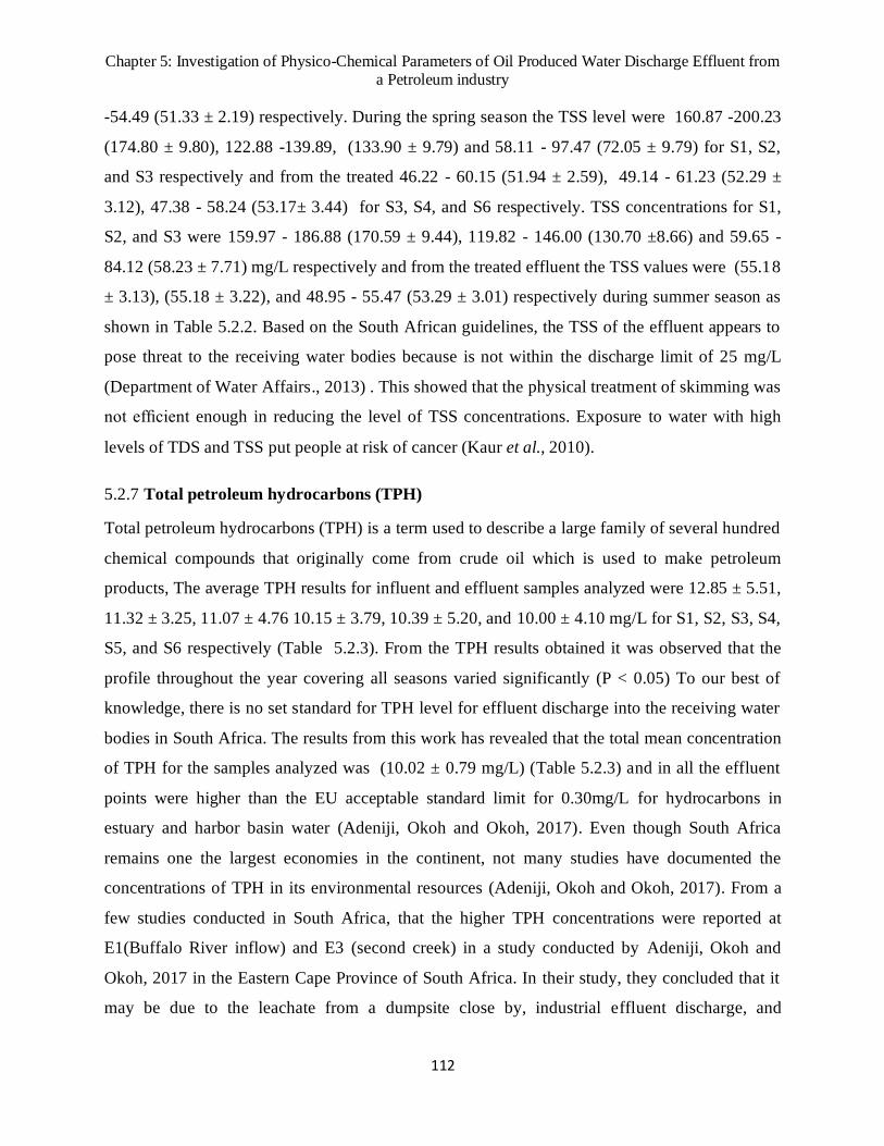
Chapter 5: Investigation of Physico-Chemical Parameters of Oil Produced Water Discharge Effluent from a Petroleum industry
112
-54.49 (51.33 ± 2.19) respectively. During the spring season the TSS level were 160.87 -200.23
(174.80 ± 9.80), 122.88 -139.89, (133.90 ± 9.79) and 58.11 - 97.47 (72.05 ± 9.79) for S1, S2,
and S3 respectively and from the treated 46.22 - 60.15 (51.94 ± 2.59), 49.14 - 61.23 (52.29 ±
3.12), 47.38 - 58.24 (53.17± 3.44) for S3, S4, and S6 respectively. TSS concentrations for S1,
S2, and S3 were 159.97 - 186.88 (170.59 ± 9.44), 119.82 - 146.00 (130.70 ±8.66) and 59.65 -
84.12 (58.23 ± 7.71) mg/L respectively and from the treated effluent the TSS values were (55.18
± 3.13), (55.18 ± 3.22), and 48.95 - 55.47 (53.29 ± 3.01) respectively during summer season as
shown in Table 5.2.2. Based on the South African guidelines, the TSS of the effluent appears to
pose threat to the receiving water bodies because is not within the discharge limit of 25 mg/L
(Department of Water Affairs., 2013) . This showed that the physical treatment of skimming was
not efficient enough in reducing the level of TSS concentrations. Exposure to water with high
levels of TDS and TSS put people at risk of cancer (Kaur et al., 2010).
5.2.7 Total petroleum hydrocarbons (TPH)
Total petroleum hydrocarbons (TPH) is a term used to describe a large family of several hundred
chemical compounds that originally come from crude oil which is used to make petroleum
products, The average TPH results for influent and effluent samples analyzed were 12.85 ± 5.51,
11.32 ± 3.25, 11.07 ± 4.76 10.15 ± 3.79, 10.39 ± 5.20, and 10.00 ± 4.10 mg/L for S1, S2, S3, S4,
S5, and S6 respectively (Table 5.2.3). From the TPH results obtained it was observed that the
profile throughout the year covering all seasons varied significantly (P < 0.05) To our best of
knowledge, there is no set standard for TPH level for effluent discharge into the receiving water
bodies in South Africa. The results from this work has revealed that the total mean concentration
of TPH for the samples analyzed was (10.02 ± 0.79 mg/L) (Table 5.2.3) and in all the effluent
points were higher than the EU acceptable standard limit for 0.30mg/L for hydrocarbons in
estuary and harbor basin water (Adeniji, Okoh and Okoh, 2017). Even though South Africa
remains one the largest economies in the continent, not many studies have documented the
concentrations of TPH in its environmental resources (Adeniji, Okoh and Okoh, 2017). From a
few studies conducted in South Africa, that the higher TPH concentrations were reported at
E1(Buffalo River inflow) and E3 (second creek) in a study conducted by Adeniji, Okoh and
Okoh, 2017 in the Eastern Cape Province of South Africa. In their study, they concluded that it
may be due to the leachate from a dumpsite close by, industrial effluent discharge, and

Chapter 5: Investigation of Physico-Chemical Parameters of Oil Produced Water Discharge Effluent from a Petroleum industry
113
urban/agricultural runoffs. Hence this study saw the necessity to include TPH as one of the
parameters to be investigated. Based on the results obtained, it is suggested that the effluents
should be subjected to secondary treatment since the primary treatment could not reduce the
contamination level and make it in allowed limit for discharge into water bodies. Secondary
treatment includes coagulation, flocculation, and further biological treatment to reduce toxicity
of petroleum wastewater (Xu and Zhu, 2004 ; Viggi et al., 2015; Changmai et al., 2017).
5.3 Prediction of compliance of oil produced water using the evaporation rate patterns.
Evaporation is a very important component of the hydrological cycle. Estimates of evaporation
rates from open water bodies are required in water resource management for multiplicity
purposes. Some examples of the application of evaporation rates include the abstraction
licensing, design of reservoirs catchment water balance studies and management of wetlands (J
W Finch and Hall, 2001). The demand for such estimates is of utmost importance in this work as
it will make it possible to use the evaporation patterns to predict the level of compliance of
wastewater that is discharged as oil produced water at an oil depot. An important step to the
understanding of evaporation is to understand the mechanisms, and therefore all the major
factors that control open water evaporation were investigated in this work.
5.3.1 Estimation of oil produced evaporation
A widely used class A pan (U.S. Department of Commerce 1970), was employed in this study to
measure the rates of evaporation. Two class A pans were installed in the field and one of pan was
filled, with clearwater (control) and the other with oil produced water (OPW). The former was
installed to measure the clear water evaporation (CWE) and the latter oil produced evaporation
(OPWE). The environmental parameters that were investigated included EC, TDS and water
temperature and they were measured from both the clearwater and OPW pans.
It should be noted that, very rarely pan evaporation measurement are used directly as estimates
of evaporation from water body because of the scale discrepancy affecting the ambient sensible
heat fluxes (J. W. Finch and Hall, 2001; Izady et al., 2016). The use of data obtained from the
pans situated away from the water body could result in considerable errors (Winter, 1981). Due
to this, the correction factor need to be applied by multiplying the observed yearly total pan

Chapter 5: Investigation of Physico-Chemical Parameters of Oil Produced Water Discharge Effluent from a Petroleum industry
114
evaporation by an empirical "pan factor" which, is approximately 0.7 as in the case of the
American class A pan as suggested by (Webb, 1966).
5.3.2 Clear water evaporation (CWE) v/s oil produced water evaporation (OPWE)
The main aim for this work was to use the evaporation patterns to predict compliance of effluents
discharged from OPW. CWE was used as reference for control purposes. The results depicted in
Figure 5.1 show that the mean evaporation rate for clear water (x = 3.98 mm/day) and this was
found to be significantly more than the evaporation from effluent from the discharge point
compartment (x = 1.94 mm/day). The clear water evaporation rate was found to be 2-fold higher
than the evaporation rates for the OPW.

Chapter 5: Investigation of Physico-Chemical Parameters of Oil Produced Water Discharge Effluent from a Petroleum industry
115
Fig. 5.1 Variation trends of CWE and OPWE for the period from May to December 2019

Chapter 5: Investigation of Physico-Chemical Parameters of Oil Produced Water Discharge Effluent from a Petroleum industry
116
The evaporation of a liquid is due to the movement of molecules from the surface into the vapor
phase above it. There are many factors which contribute to the rate of the evaporation of the
liquid. Figure 5.1 shows the relation of proportionality between CWE and OPWE. However, the
CW shows to evaporate more than OPW. This observation agrees with literature because
theoretically, oil do not mix with water and oil is less dense than water (including the crude oils).
Therefore, this will cause the oil to float on top of the water and form a thin layer depending on
the type of the oil thus hindering the evaporation of the liquid water underneath. Light oils
changes drastically from fluid to viscous and Heavy oils becomes solid-like (Fingas, 2015). This
resulted in the evaporation of OPWE to be lower than that for CWE.
5.3.3 Effect of the climatic parameters on the rate of evaporation
Evaporative demand is measured directly by Epan (evaporation from the pan) (Roderick et al.,
2007) and is mostly strongly influenced by climatic parameters which include solar irradiance,
temperature, humidity and wind speed (Roderick and Farquhar, 2002; Roderick et al., 2007). The
climatic/meteorological factors that have notable effects on the evaporation process are air
temperature, water temperature, solar radiation, and wind speed.
5.3.4 Air temperature (Ta)
Statistical analysis of the results for air temperature measurements (Figure 5.2) using ANOVA
revealed that in most cases, there were significant differences (P<0.05) in air temperature
throughout the study with the mean air temperature being (x = 20.20° C) (Table: 5.2.4).

Chapter 5: Investigation of Physico-Chemical Parameters of Oil Produced Water Discharge Effluent from a Petroleum industry
117
Table 5.2.4: Annual variation of the evaporation and climatic parameters.
parameters Mean SD
CWE (mm/da) 3.98 1.51
OPWE (mm/day) 1.94 0.86
Ta (°C) 20. 20
5.93
Tcwe (°C) 25.37 6.66
Topw 28.08 6.71
W (m/s) 3.23 0.92
R (W/m2) 6.20 2.04

Chapter 5: Investigation of Physico-Chemical Parameters of Oil Produced Water Discharge Effluent from a Petroleum industry
118
Figure 5.2: Variation trends of monthly evaporation rates vs air temperature for the period
of May to December 2019
Variation trends of monthly evaporation rates vs air temperature for the period from May
toDecember2019.

Chapter 5: Investigation of Physico-Chemical Parameters of Oil Produced Water Discharge Effluent from a Petroleum industry
119
Figure 5.2 shows that there is a directly proportional relationship between the evaporation rates
and the air temperature. Figure 5.2 depicts the monthly effluent evaporations for the period
covering May – December 2019. The magnitude of evaporation was at its maximum in spring
(September to November) and summer (December) and low in June – August 2019 because
South Africa has typical weather of the Southern Hemisphere, with the coldest days in June–
August. The rising trends of air temperature from September to December resulted into increased
rates of evaporation. This is because higher temperature results into movement of more
molecules from the bottom to the water surface with high speed thus causing increasing escape
as vapor and furthermore high temperature causes intensive molecule diffusion into surrounding
space (Vuglinsky, 2009).
5.3.5 Solar radiation
Figure 5.3 shows that the evaporation rates varied significantly over the open-water season
throughout the year of the study (P<0.05), and the pattern of variation was not consistent from
month to month.

Chapter 5: Investigation of Physico-Chemical Parameters of Oil Produced Water Discharge Effluent from a Petroleum industry
120
Figure 5.3: Variation trends of monthly evaporations and solar radiation for the period of
May to December 2019.

Chapter 5: Investigation of Physico-Chemical Parameters of Oil Produced Water Discharge Effluent from a Petroleum industry
121
There’s a harmonious relationship between solar radiation and the evaporation rates, that is, the
rate of evaporation of OPW and CW increased with the increase in the solar radiation intensity
(Figure 5.3). This trend and observation can be explained from the fact that, solar radiation is a
source of energy to molecules and thus the higher the solar radiation bombarding the water
surface tends to increase the kinetic energy in order to overcome forces of cohesion thus
resulting in the increased evaporation rates The results depicted in Figure 5.3 show that the
evaporation rates were at its maximum when the solar radiation was high though not in the same
order of magnitude. Based on the total mean of CWE and OPWE of 3.98 and 1.94 mm/day
respectively (Table 5.2.4), the CWE was found to be at 2-fold higher than that of OPWE. This
observation is fully logical, because solar radiation can penetrate at greater depth enhancing the
evaporation rates of clear water whereas, the layer on top of the OPW hindering the solar
radiation penetration which results in lower evaporation rates compared to that of clear water.
Lower evaporation rates were observed when the solar radiation was at its minimum implying
that during the evaporation process, not enough energy reached water, therefore the water cooled
and resulted in lower evaporation rates.
5.3.6 Wind speed
Figure 5.4 depicts the results obtained that indicate the relationship between the wind speed (W)
and the rate of evaporation.

Chapter 5: Investigation of Physico-Chemical Parameters of Oil Produced Water Discharge Effluent from a Petroleum industry
122
Figure 5.4: Variation trends of monthly evaporations and wind speed for the period of May to
December 2019.
The relationship between wish speed seem to be directly proportional to the evaporation rates.
Wind speed values were greater in the dry summer months than the winter months (Figure 5.4).
This observations was similar to that reported by Hoffman et al., (2011) whereby in their study
where they investigated the changes in Epan, wind speed, rainfall, temperature, and vapor-
pressure deficit from 1974 to 2005 taken from 20 climate stations in the Cape Floristic Region
(CFR), South Africa. They further suggested that the Epan reduction was likely due to the
decrease in wind speed. In addition, this study has found that, no statistical significance detected
for wind speed throughout the period (p<0.05).

Chapter 5: Investigation of Physico-Chemical Parameters of Oil Produced Water Discharge Effluent from a Petroleum industry
123
5.3.7 Water temperature (Tw)
Figure 5.5 indicates how the water temperature affects the rates of evaporation.
0
0,1
0,2
0,3
0,4
0,5
0,6
0,7
0,8
0,9
1
0
0,1
0,2
0,3
0,4
0,5
0,6
0,7
0,8
0,9
1
Wat
er t
emp
erat
ure
evap
ora
tio
n (
mm
/day
)
Period (Months)
CWE (mm/day)
OPWE (mm/day)
CWE Tpan (°C)
Topw pan (°C)
Figure 5.5: Variation trends of monthly evaporations and water temperature for the period of
May to December 2019.
The trend observed suggest that the rate of evaporation tend to increase with an increase in water
temperature (Figure 5.5). This is because the water molecules move rapidly when heated thus
making the water molecules to escape faster. Higher temperatures lead to increase
in vaporization as more molecules get kinetic energy to convert into vapor and then escape. The
evaporation rates of clear water were less during winter ( June – August) due to the water
becoming cooler however the same trend was not observed for oil produced water because waste
water has the ability to store energy thus the evaporation rates of oil produced water were high
during winter ( June- July).

Chapter 5: Investigation of Physico-Chemical Parameters of Oil Produced Water Discharge Effluent from a Petroleum industry
124
5.4 Effect of the climatic parameters on the rate of evaporation
Environmental factors effecting evaporation process including EC, TDS, TSS, TOC, COD, BOD
and TPH are discussed below:
5.4.1 Total dissolved solids (TDS)
The influence of TDS was investigated, and the results are depicted in Figure 5.6

Chapter 5: Investigation of Physico-Chemical Parameters of Oil Produced Water Discharge Effluent from a Petroleum industry
125
Figure 5.6: Variation trends of monthly evaporations and total dissolved solids for the
period of May to December 2019.
Figure 5. 6 shows the variations of TDS relative to the evaporation rate. This study found that,
the TDS measure was directly proportional to the rate of evaporation. This observation can be
explained from the fact that the more the ions are present in water the higher the absorption of
solar radiation which is a source of energy to molecules giving them enough energy escape the
surface. The elevated level of TDS was observed during summer thus leading to high level of
OPWE.
Statistical analysis using ANOVA revealed that there were significant differences (P<0.05) in
TDS values throughout the study.
Figure 5.6: Variation trends of monthly evaporations and total dissolved solids for the period of
May to December 2019.
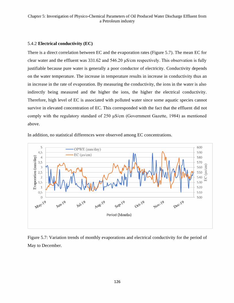
Chapter 5: Investigation of Physico-Chemical Parameters of Oil Produced Water Discharge Effluent from a Petroleum industry
126
5.4.2 Electrical conductivity (EC)
There is a direct correlation between EC and the evaporation rates (Figure 5.7). The mean EC for
clear water and the effluent was 331.62 and 546.20 μS/cm respectively. This observation is fully
justifiable because pure water is generally a poor conductor of electricity. Conductivity depends
on the water temperature. The increase in temperature results in increase in conductivity thus an
in increase in the rate of evaporation. By measuring the conductivity, the ions in the water is also
indirectly being measured and the higher the ions, the higher the electrical conductivity.
Therefore, high level of EC is associated with polluted water since some aquatic species cannot
survive in elevated concentration of EC. This corresponded with the fact that the effluent did not
comply with the regulatory standard of 250 μS/cm (Government Gazette, 1984) as mentioned
above.
In addition, no statistical differences were observed among EC concentrations.
Figure 5.7: Variation trends of monthly evaporations and electrical conductivity for the period of
May to December.

Chapter 5: Investigation of Physico-Chemical Parameters of Oil Produced Water Discharge Effluent from a Petroleum industry
127
5.4.3 Organic carbons (BOD, COD, and TOC)
The maximum values of the organic carbons were observed in summertime with the mean of
3.21, 249.39, 130.00 ,160.00 mg/L for S1, S2 and S3 respectively. Figure 5.8 shows an empirical
relationship between the evaporation rates and the organic matter parameters. The higher the
organic content or carbon , the more oxygen is consumed. A high organic content implies the
increase in the growth of microorganisms which contribute to the depletion of oxygen supplies.
The trend suggests that the reduction in the evaporation rate results in the reduction of
pathogenic microorganisms. This observation is genuine because it is known that aquatic
bacterioplankton are sensitive to sunlight radiation, especially in the shortest-wavelength
fraction of UV radiation (Herndl, Mi and Frick, 1993) (Sommaruga et al., 1997)(Sommaruga et
al., 2005)(Alonso-Sáez et al., 2006). Moreover, Alonso-Sáez et al., (2006) conducted a study to
investigate the effects of natural sunlight on heterotrophic marine bacterioplankton and the
results suggested that UV radiation can significantly affect the in-situ single-cell activity of
bacterioplankton and the naturally dominating phylogenetic bacterial groups have different
sensitivity to natural levels of incident solar radiation. Surface solar radiation levels also
photochemically degrade bacterial extracellular enzymes. Therefore, increased UV-B radiation
due to the destruction of the stratospheric ozone layer might have led to a reduced bacterial
activity and the corresponding increased concentration of labile dissolved organic matter in the
surface layers of the ocean as bacterial uptake of this is retarded (Herndl, Mi and Frick, 1993).

Chapter 5: Investigation of Physico-Chemical Parameters of Oil Produced Water Discharge Effluent from a Petroleum industry
128
Figure 5.8: Variation trends of monthly evaporations and organic matter parameters for the
period of May to December 2019.
5.4.4 Total suspended solids (TSS)
As stated earlier, the TSS concentration varied significantly (p<0.05). This study has also found
that, the rate of the evaporation for both CW and OPW was proportional to the TSS
concentrations. The TSS values were high during summer (September to November 2019)
season as pointed out above thus leading to more absorption of solar radiation hence the rise in
temperature which resulted into the elevated evaporation rates. Therefore, high level of TSS is
associated with polluted water since elevated level of TSS may settle out onto a lake or
streambed bottom and cover aquatic organisms, eggs, or macro-invertebrate larva (Whitman
College, 2015). This coating can prevent enough oxygen transfer a which may lead to the death
of buried organisms. Its formation is dependent primarily on the physical processes driven by
hydrological phenomena. This corresponded with the fact that the effluent didn’t comply with
the regulatory standard of 25 mg/L (Department of Water Affairs, 2013) as mentioned above.
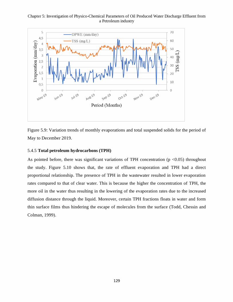
Chapter 5: Investigation of Physico-Chemical Parameters of Oil Produced Water Discharge Effluent from a Petroleum industry
129
Figure 5.9: Variation trends of monthly evaporations and total suspended solids for the period of
May to December 2019.
5.4.5 Total petroleum hydrocarbons (TPH)
As pointed before, there was significant variations of TPH concentration (p <0.05) throughout
the study. Figure 5.10 shows that, the rate of effluent evaporation and TPH had a direct
proportional relationship. The presence of TPH in the wastewater resulted in lower evaporation
rates compared to that of clear water. This is because the higher the concentration of TPH, the
more oil in the water thus resulting in the lowering of the evaporation rates due to the increased
diffusion distance through the liquid. Moreover, certain TPH fractions floats in water and form
thin surface films thus hindering the escape of molecules from the surface (Todd, Chessin and
Colman, 1999).

Chapter 5: Investigation of Physico-Chemical Parameters of Oil Produced Water Discharge Effluent from a Petroleum industry
130
Figure 5.10: Variation trends of monthly evaporations and total suspended solids for the period
of May to December 2019.

Chapter 5: Investigation of Physico-Chemical Parameters of Oil Produced Water Discharge Effluent from a Petroleum industry
131
5.4.6 Comparison with literature data
The values for various physicochemical parameters for OPW obtained from this work, was
compared with others reported in the literature. Table 5.3 shows this comparison, whereby the
values from this work are in some cases very different from some values previously reported.
This was expected and can be attributed from the fact that, the chemistry of OPW from different
industries will present different characteristics and properties as they will be characteristic to that
industry or geographical location.

Chapter 5: Investigation of Physico-Chemical Parameters of Oil Produced Water Discharge Effluent from a Petroleum industry
132
Table 5.3: Comparison of petroleum effluent data from present study with data from previous studies
Effluent
characteristics
Sources
Demirci et al.,
(1998)
Zenga et al.,
(2007)
Dincer et al.,
(2008)
Saber et al.,
(2014)
(Varjani, Kumar and
Rene (2019)
This
work
pH 6.5-8.5 6.5-6.8 2.5 6.7 6.0-8.5 -
Chemical oxygen
demand
800.00 500-1000 21000 450.00 125.00 249.74
Biochemical oxygen
demand
350.00 - 8000.00 174.00 15.00 3.01
Total suspended
solids
150.00 3000-5000 2580.00 150.00 20.00 49.81
Total dissolved solids - 37000.00 6200.00
Total organic carbon - - - 119.00 - 125.25
Oil and Grease 3000.00 400-1000 1140.00 870.00 5 -
Lead - - - - 0.01 -
Nickel - - - - 1 -
Zinc - - - - 5 -
Copper - - - - 1 -
Mercury - - - - 0.01 -
Benzene - - - - 0.1 -
Sulphides 17 15-30 - - 0.5 -

Chapter 5: Investigation of Physico-Chemical Parameters of Oil Produced Water Discharge Effluent from a Petroleum industry
133
5.5 The correlation studies
The correlations among the physicochemical properties were examined throughout the project.
Air temperature didn’t show any significant correlation with electrical conductivity of both clear
water and oil produced water and TDS of clearwater and TOC. However, a strong correlation
was observed between wind speed, solar radiation, Clear water temperature, OPWE, oil
produced temperature (Topw), TDS of oil produced water, COD, TSS ( r = 0.33, 0.45, 0.58,
0.33, 0.56, 0.64, 0.35 0.48, P<0.05 respectively) and air temperature with TPH exhibited a
negative correlation (-0.34). Wind speed showed no correlation with environmental parameters
except for BOD ( r = 0.26, P < 0.05) and it also showed a positive correlation with the climatic
parameters, mainly solar radiation, CWE, clear water temperature, oil produced temperature,
clear water TDS (0.30, 030, 0.23, 0.22, 0.22; p<0.05). Generally, there was a correlation between
climatic parameters and environmental parameters with the rate of both clearwater and oil
produced water. It was then necessary to perform the correlation study in order to understand the
nature of investigated parameters and their species speciation in the effluent and receiving
waterbody as well as to use the evaporation pattern to predict compliance of the targeted
wastewater. The results for a correlation study are shown in Table 5.2.

Chapter 5: Investigation of Physico-Chemical Parameters of Oil Produced Water Discharge Effluent from a Petroleum industry
134
Table 5.2.4: Correlation coefficient r for different parameters from the study period
Parameter Tair (°C) W (m/s) R (W/m²) CWE
(mm/day)
Tcwe(°C) ECcwe
(μs/cm)
TDScwe
(mg/L)
OPWE
(mm/day)
Topw
(°C)
TDSopw
(mg/L)
ECopw
(μs/cm)
BOD
(mg/L)
COD
(mg/L)
TOC
(mg/L)
Tair (°C) 1.00
W (m/s) 0.33 1.00
R (W/m²) 0.45 0.30 1.00
CWE
(mm/day)
0.58 0.30 0.28 1.00
Tcwe (°C) 0.33 0.23 -0.25 0.56 1.00
ECcwe
(μS/cm)
-0.07 0.16 0.02 0.04 0.13 1.00
TDScwe
(mg/L)
0.13 0.22 0.05 0.22 0.23 0.31 1.00
OPWE
(mm/day)
0.56 0.15 0.14 0.82 0.54 -0.06 0.20 1.00
Topw (°C) 0.64 0.22 0.14 0.63 0.58 0.05 0.22 0.56 1.00
TDS (mg/L) 0.49 0.18 -0.10 0.57 0.71 0.02 0.31 0.58 0.71 1.00
EC (μS/cm) 0.12 0.07 -0.04 0.26 0.33 0.19 0.10 0.15 0.52 0.43 1.00
BOD
(mg/L)
0.19 0.26 -0.11 0.28 0.55 0.05 0.13 0.40 0.20 0.50 0.16 1.00
COD
(mg/L)
0.35 -0.05 0.37 0.16 -0.12 -0.30 -0.20 0.21 0.08 -0.06 -0.10 0.18 1.00
TOC
(mg/L)
-0.01 0.05 -0.12 0.09 0.18 0.04 0.00 0.19 -0.04 -0.06 0.09 0.38 0.11 1.00
TSS (mg/L) 0.48 0.11 0.10 0.55 0.53 -0.09 0.07 0.61 0.76 0.67 0.33 0.35 0.26 -0.10
TPH (mg/L) -0.34 0.00 -0.19 -0.19 -0.05 0.09 0.03 -0.05 -0.30 -0.16 -0.14 0.36 -0.04 0.14

Chapter 5: Investigation of Physico-Chemical Parameters of Oil Produced Water Discharge Effluent from a Petroleum industry
135
OPWE: oil produced water; CWE: clear water evaporation; Tair: air temperature; R: solar
radiation, W: wind speed; Topw: oil produced water temperature; Tcwe: clear water temperature;
Topw : oil produced water temperature; ECcwe electrical conductivity of clear,water; ECopw:
electrical conductivity of oil produced water ; TDScwe: total dissolved solids of clear water;
TDSopw: total dissolved solids of oil produced water; TSS: total suspended solids; BOD:
biological oxygen demand; COD: chemical oxygen demand; TOC: total organic carbon; TPH:
total petroleum hydrocarbon.

Chapter 5: Investigation of Physico-Chemical Parameters of Oil Produced Water Discharge Effluent from a Petroleum industry
136
5.6 Conclusion
Physico-chemical parameters of the effluents from the oil depot were assessed in this study.
Most of the parameters were within the acceptable threshold limits except for COD, TPH and EC
that slightly surpassed. This means that wastewater from this oil depot should not be directly
discharged into municipal channels, rivers and streams unless it undergoes secondary and tertiary
treatment processes. Alternatively, the wastewater may under agreement be channelled to local
municipality for further treatment since most depot do not have appropriate facilities for post-
treatment process; however, the chemical effluent must also adhere to the rules guidelines and
regulations of the municipal where the wastewater will be channelled into. Another challenge,
will be the large volume of the wastewater generated being and channelled elsewhere since they
contain a lot of by-products. The majority of the oil depots employ physical treatment processes
which as it proved by the obtained results are not always effective also do not have necessary
equipment to check compliance of the chemical effluent. Therefore, this study sought to use the
evaporation patterns to predict the compliance of such wastewater. Based on the results obtained,
it is possible to use the evaporation pattern. The evaporation and correlation study supported the
hypothesis. As shown by the evaporation patterns that most of the time the effluent was
compliant mostly in winter time than summer time, and this observation was explained by the
evaporation patterns that in summer when there is more solar radiation, the wastewater absorbed
more heat and enhanced the evaporation rates which is directly related to both environmental and
climatic parameters.

Chapter 5: Investigation of Physico-Chemical Parameters of Oil Produced Water Discharge Effluent from a Petroleum industry
137
5.7 References
Adeniji, A. O., Okoh, O. O. and Okoh, A. I. (2017) ‘Petroleum Hydrocarbon Fingerprints of
Water and Sediment Samples of Buffalo River Estuary in the Eastern Cape Province , South
Africa’, Journal of Analytical Methods in Chemistry, pp. 1–13.
Alonso-Sáez, L., Gasol, J.M. Lefort, T. Hofer, J. and Sommaruga, R. (2006) ‘Effect of natural
sunlight on bacterial activity and differential sensitivity of natural bacterioplankton groups in
Northwestern Mediterranean coastal waters’, Applied and Environmental Microbiology, 72(9),
pp. 5806–5813. doi: 10.1128/AEM.00597-06.
Aniyikaiye, T. E., Oluseyi,T. Odiyo, J.O and Edkpayi, J.N. (2019) ‘Physico-Chemical Analysis
of Wastewater Discharge from Selected Paint Industries in Lagos , Nigeria’, International
Journal oF Environmental Research and Pu, 16, pp. 1–17. doi: 10.3390/ijerph16071235.
Bennett, G. F. and Peters, R. W. (1988) ‘The removal of oil from wastewater by air flotation: A
review’, Critical Reviews in Environmental Control, 18(3), pp. 189–253. doi:
10.1080/10643388809388348.
Bhateria, R. and Jain, D. (2016) ‘Water quality assessment of lake water: a review’. Springer
International Publishing, 2(2), pp. 161–173. doi: 10.1007/s40899-015-0014-7.
Changmai M, Pasawan M, Purkait MK (2017) ‘Treatment of oily wastewater from drilling site
using electrocoagulation followed by microfiltration’. Seperation and Purification Technology
210. pp, 463–472
Demicrci S., Erdogan B. and Oezcicmder R. (1998) ‘Wastewater treatment at the petroleum
refinery, Kirikale, Turkey using some coagulants and Turkish clays as coagulant aids’, Water
Res., 32, pp. 3495-3499.
Dincer A.R., Karakaya N., Gunes E. and Gunes Y. (2008) ‘ Removal of COD from oil recovery
industry wastewater by the Advanced Oxidation Processes (AOP) based on H2O2, Glob. N. J’
10, pp. 31-38.
Department of Water Affairs. (2013) Revision of general authorisations in terms of Section 39 of
Chapter 5: Investigation of Physico-Chemical Parameters of Oil Produced Water Discharge Effluent from a Petroleum industry
138
the National Water Act, 1998 (Act No. 36 of 1998), No. 665. Government Gazette No. 36820, 6
September. Department of Water Affairs, Pretoria, South Africa.
Edokpayi, J. N., Odiyo, J. O. and Durowoju, O. S. (2017) Impact of Wastewater on Surface
Water quality in Developing Countries: A study of South Africa, Water Quality. Chapter 18.
Intech. doi: http://dx.doi.org/10.5772/57353.
Ehiagbonare, J. E. and Ogunrinde, Y. O. (2010) ‘Physico-chemical analysis of fish pond water in
Okada and its environs , Nigeria’, African Journal of Biotechnology, 9(36), pp. 5922–5928.
Farajnezhad, H. and Gharbani, P. (2012) ‘Coagulation Treatment of Wastewater in Petroleum
Industry using Poly Aluminium Chloride and Ferric’, International Journal of Recent Research
and Applied Studies, 13(1), pp. 306–310.
Fatoki, O. S., Gogwana, P. and Ogunfowokan, A. O. (2003) ‘Pollution assessment in the
Keiskamma River and in the impoundment downstream’, Water SA, 29(2), pp. 183–187. doi:
10.4314/wsa.v29i2.4854.
Finch, J W and Hall, R. L. (2001) Estimation of Open Water Evaporation.
Fingas, M. (2015) ‘Oil and Petroleum Evaporation’, in Handbook of Oil Spill Science and
Technology, pp. 205–223. doi: 10.1002/9781118989982.ch7.
Government Gazette (1984) Requirements for the Purification of Wastewater or Effluent.
Gazette No 9225, Regulation No 991, 18 May.
Hanafy, M. and Nabih, H. I. (2007) ‘Treatment of oily wastewater using dissolved air flotation
technique’, Energy Sources, Part A: Recovery, Utilization and Environmental Effects, 29(2), pp.
143–159. doi: 10.1080/009083190948711.
Havard, D. (2013) Oil and Gas Production Handbook - An introduction to oil and gas
production, transport, refining and petrochemical industry.
Herndl, G. J., Mi, G. and Frick, J. (1993) ‘Major role of ultraviolet-B in controlling
bacterioplankton growth in the surface layer of the ocean’, N, 361(February), pp. 717–719.
Hoffman, M. T., Cramer, M.D. Gillson, L. and Wallace, M. (2011) Pan evaporation and wind
run decline in the Cape Floristic Region of South Africa ( 1974 – 2005 ): implications for
Chapter 5: Investigation of Physico-Chemical Parameters of Oil Produced Water Discharge Effluent from a Petroleum industry
139
vegetation responses to climate change. doi: 10.1007/s10584-011-0030-z.
Igbinosa, E. O. and Okoh, A. I. (2009) ‘Impact of discharge wastewater effluents on the physico-
chemical qualities of a receiving watershed in a typical rural community’, International Journal
of Environmental Science and Technology, 6(2), pp. 175–182.
Izady A., Abdalla, O., Sadeghi, M., Majidi, M,. Karimi, A., and Chen M., (2016). Novel
Approach to Modeling Wastewater Evaporation Based on Dimensional Analysis, Water
Resources Management. Water Resources Management, 30, pp. 2801–2814. doi:
10.1007/s11269-016-1324-8.
Jirka, A. M. and Carter, M. J. (1975) ‘Micro Semi-Automated Analysis of Surface and Waste
Waters for Chemical Oxygen Demand’, Analytical Chemistry, 47(8), pp. 1397–1402. doi:
10.1021/ac60358a004.
Kaur, A., Vats,S. Rekhi, S. Bhadwaj, A. Goel, J. Tanwar, R.S. Gaur, K.K. (2010) ‘Physico-
chemical analysis of the industrial effluents and their impact on the soil microflora’, in Procedia
Environmental Sciences, 2, pp. 595–599. doi: 10.1016/j.proenv.2010.10.065.
Li, X., Cao, X. Wu, G. Temple, T. Coulon, F. and Sui, H. (2014) ‘Ozonation of diesel-fuel
contaminated sand and the implications for remediation end-points’, Chemosphere. Elsevier Ltd,
109, pp. 71–76. doi: 10.1016/j.chemosphere.2014.03.005.
Padaki, M., Murali. R.S. Abdullah, M.S. Misdan, N. Moslehyani, A. Kassim, M.A Hilal, N and
Ismail, A.F. (2015) ‘Membrane technology enhancement in oil-water separation. A review’,
Desalination. Elsevier B.V., 357, pp. 197–207. doi: 10.1016/j.desal.2014.11.023.
Roderick, M.L. and Farquhar, G.D (2002) ‘ The cause of decreased pan evaporation over the past
50 years’.Science, 298, pp. 1410–1411.
Roderick, M.L, Rotstayn, L.D, Farquhar G.D, Hobbins, M.T. (2007) ‘On the attribution of
changing pan evaporation. Geophys Res Lett, 34, pp.251–270.
U.S. Department of Commerce (1970) Climatological Summary. Brownsville, Texas, pp. 46
Saber A., Hasheminejad H. Taebi A. and Ghaffari G. (2014) ‘Optimization of Fenton-based
treatment of petroleum refinery wastewater with scrap iron using response surface methodology’

Chapter 5: Investigation of Physico-Chemical Parameters of Oil Produced Water Discharge Effluent from a Petroleum industry
140
Applied Water Science, 4, pp. 283-290.
Samudro, G. and Mangkoedihardjo, S. (2014) ‘Review on BOD , COD and BOD / COD ratio : a
triangle zone for toxic , biodegradable and stable levels’, International Journal Of Academic
Research, 2(4), pp. 235–239.
Sommaruga, R., Obernosterer, I. Herndl, G.J And Psenner, R. (1997) ‘Inhibitory effect of solar
radiation on thymidine and leucine incorporation by freshwater and marine bacterioplankton’,
Applied and Environmental Microbiology, 63(11), pp. 4178–4184. doi: 10.1128/aem.63.11.4178-
4184.1997.
Sommaruga, R., Hofer, J.S. Alonso-Sa´ez, L and Gasol, J.M (2005) ‘Differential sunlight
sensitivity of picophytoplankton from surface Mediterranean coastal waters’, Applied and
Environmental Microbiology, 71(4), pp. 2154–2157. doi: 10.1128/AEM.71.4.2154-2157.2005.
Sonune, A. and Ghate, R. (2004) ‘Developments in wastewater treatment methods’, in
Desalination, pp. 55–63.
Todd, G. D., Chessin, R. L. and Colman, J. (1999) Toxilogical Profile for Total Petroleum
Hydrocarbons (TPH). Public Health.
Varjani S, Kumar G, Rene ER (2019) ‘Treatment of wastewater from petroleum industry: current
practices and perspectives’, Environmental Science and Pollution Research, pp. 1–9. doi:
10.1007/s11356-019-04725-x.
Varjani, S. J. and Upasani, V. N. (2017) ‘A new look on factors affecting microbial degradation
of petroleum hydrocarbon pollutants’, International Biodeterioration and Biodegradation.
Elsevier Ltd, 120, pp. 71–83. doi: 10.1016/j.ibiod.2017.02.006.
Viggi, C. C. Presta, E. Bellagamba, M. Kaciulis, S. Balijepalli, S.K. Zanaroli, G. Papini, P.M.
Rossetti, S. Aulenta, F. (2015) ‘The BOil Spill Snorkel^: an innovative bioelectrochemical
approach to accelerate hydrocarbons biodegradation in marine sediments’ Frontiers in
Microbiology. 6 (881), pp. 1–11. https://doi.org/10.3389/fmicb.2015.00881
Vuglinsky, V. S. (2009) ‘Evaporation From Open Water Surface And Groundwater’
Hydrological Cycle.

Chapter 5: Investigation of Physico-Chemical Parameters of Oil Produced Water Discharge Effluent from a Petroleum industry
141
Webb, E. K. (1966) ‘A pan-lake evaporation relationship’, Journal of Hydrology, 4, pp. 1–11.
doi: 10.1016/0022-1694(66)90063-1.
Whitman College (2015) ‘Total Suspended Solids in Water Samples’, Available at:
https://www.whitman.edu/chemistry/edusolns_software/TSSBackground.pdf.
Wirnkor, V. A. Amonia, B. O. and Ngozi, V. E. (2014) ‘Batch and Column Adsorption of BOD
and COD in Vegetable Oil Industry Effluents Using Activated Carbon from Fluted Pumpkin
(Telfairia, Occidentalis. Hook. F) Seed Shell’, International Letters of Chemistry, Physics and
Astronomy, 39, pp. 64–77. doi: 10.18052/www.scipress.com/ilcpa.39.64.
Winter, T.C. and Rosenberry, D.O. (1995) ‘Evaluation of 11 equations for determining
evaporation for a small lake in the north central United States’ Water Resource Research, 31(4),
pp. 983-993.
Xu, X. and Zhu, X. (2004) ‘Treatment of refectory oily wastewater by electro-coagulation
process’, Chemosphere, 56, pp. 889–894. doi: 10.1016/j.chemosphere.2004.05.003.
Zenga ,Y., Yang C. Zhang J. and Pu W. (2007) ‘ Feasibility investigation of oily wastewater
treatment by combination of zinc and PAM in coagulation/flocculation, Journal of Hazardous
Materials’ 147, pp. 991-96.

142
CHAPTER 6 : DEVELOPMENT OF THE OIL PRODUCED WATER
MODEL TO BE USED FOR ASCERTAINING THE COMPLIANCE TO
GUIDELINES
The chapter focuses on the development and implementation of a model to be as an indicator of a
pollution caused by the oil produced water and be used as a predictive tool for cases of non-
compliance. The results obtained in the previous chapter (chapter 5) were applied to develop a
multiplicative model. The details on the development of the model using the rate of evaporations
patterns will be discussed in detail.
6.1 Introduction
With the advancement of technology and industrial growth, the contamination of freshwater
resources has become a global issue. The world is observing an increase in urbanization and
industrialization due to the consumerist approach (Li and Yu, 2011; Zhang et al., 2015). Water
quantity is as important as water quality and therefore both aspects need to be given the due
weight. This means that the strategies of minimizing industrial waste need to be implemented.
Managing environmental pollution is a legal requirement, and one of the ways of managing it is
to ensure the wastewater discharged from industries do not cause harmful damages to the
environment. Normally, laboratory testing of collected samples is one way to ensure that the
chemical composition of the effluent meet the stipulated discharge limits enforced by the
regulators. However, this might be a challenge for many oilfields because it is time consuming,
expensive (since many oilfields do not have laboratories with relevant equipment to analyze the
effluents), and moreover some testing techniques and approaches may even lead to secondary
pollution because some tests involve the use of toxic chemicals and reagents. Therefore, this
study explored the possibility of developing a model using dimensional analysis to predict the
compliance of the effluent.
Oil produced water evaporation (OPWE) is highly nonlinear in nature, thus prompting the search
for models that are capable of addressing this tendency of non-linearity’s in the process since it
cannot be directly ascertained but only estimated depending on either the energy or water budget

Chapter 6: Development of the Oil Produced Water Model
143
or mass transfer approaches (Sudheer et al., 2002). Thus, dimensional analysis based on
Buckingham π theorem was employed for this study.
6.2 Model development based on Buckingham pi theorem.
A model is a simplification of the reality on the ground. In general, it is a representation between
the source and a target (Sibel, 1998; Boulter and Gilbert, 1996), the target being an unknown
phenomenon or object needs to be explained, and the source being a familiar phenomenon or
object assisting the scientists to understand the target. Models play central roles in expert
scientists' reasoning and problem-solving (Clement, 1989); Chi, Feltovich and Glaser, 1981;
Larkin, 1981; Reif, 1983) and they are instrumental in summarizing data, making predictions,
justifying outcomes and facilitating communication in science. To the best of our knowledge,
there’s no model developed to predict compliance of the wastewater effluent and dimensional
analysis based on Buckingham pi theorem (Buckingham, 1914) was to be used to formulate a
multiplicative equation (equation 6.1).
(6.1)
The details of the steps for the model development have been given in Chapter 3 in section 3.8
of this dissertation
6.2.1 Obtaining the coefficients
The data collected from the oil field (May - December 2019) was randomized to minimize bias
and the coefficients were determined by regression analysis using a software known as statistical
package for the social sciences (SPSS). 70% of the data was used for calibration the coefficients
were obtained (C, α, β, γ, δ, ε, μ, ρ and ω.) and the remaining 30% was used for validation. The
reason to subdivide the data into two is because, the calibration curve is to train the data set and
the validation is for estimate prediction error in order to compare models. The data was fitted to a
nonlinear regression analysis since OPWE is nonlinear in nature. The general equation was
entered as the theoretical expression is SPSS. To determine the coefficients, SPPS was provided
with the starting value for each constant and it was then used an iterative method to change the

Chapter 6: Development of the Oil Produced Water Model
144
values of the constants to get the best fit of nonlinear expression that fits the data. Therefore, the
SPSS gave an iteration history with an iterative table indicating how many steps the iteration
takes from the starting value to the end to get the best fit results.
6.2.2 Statistical analysis
Based on the regression analysis form the statistical package for social sciences (IBM SPSS
Statistics 22), the constants of Eq. (6.1) were obtained as C=200.337, α=0.8028, β=−0.0487, γ=-
0.191, δ =1.130 , ε =0.0326 , μ= 0.707 , ρ = -1.1690 and ω = 0.157 leading to the final
mathematical model (equation 6.2) as follows:
(6.2)
Where:
OPWE is oil produced water evaporation
CWE is the clear evaporation
TDS is the total dissolved solids
TSS is the total suspended solids
EC is the electrical conductivity
Ta is the air temperature
R is the solar radiation
W is the wind speed
Topw is the oil produced water temperature
TPH is total petroleum hydrocarbon
COD is chemical oxygen demand
BOD is biological oxygen demand
TOC is the total organic carbon

Chapter 6: Development of the Oil Produced Water Model
145
6.2.3 Estimation of OPWE using dimensional analysis results
From the calibration data set, the estimated OPWE was obtained by fitting the coefficients values
to equation (6.2) and statistical chemometrics used to characterize the external predictivity of a
model were coefficient of determination (R2), and relative mean absolute error (RMSE) in order
to evaluate the effectiveness and the accuracy of the proposed method. These chemometrics were
calculated using OPWE measured and OPWE estimated. The data was randomized until the best
randomized set of data was obtained with high R2 and low RMSE. From the validation data set
the OPWE estimated was calculated and the chemometrics methods were also be calculated
using OPWE measured and OPWE estimated (Table: 6.1).
Table 6.1: Statistical chemometrics of the proposed method
Phase R2 RMSE (mm/day) MAE
calibration 0.70 0.49 0.33
validation 0.73 0.47 0.35
6.2.4 (Coefficient of determination R2)
R2 is generally defined as the square of the correlation coefficient between observed and
predicted values in a regression (Alexander, Tropsha and Winkler, 2015). The aim of the
coefficient of determination analysis was to determine how well the model fits the data. As Table
6.1 showed, the regression model for calibration accounted for 70% of the variance which can be
explained by the entire data set of dependent variables while for validation purpose it accounted
for 73%. This suggest that the more variance that is accounted for by the regression model the
closer the data points will fall to the fitted regression line. Moreover, derived equation fairly
predicts the oil produced evaporation. The R2 obtained in this study is similar to the one reported
for modelling wastewater evaporation using dimensional analysis in Oman ((Izady et al., 2016).

Chapter 6: Development of the Oil Produced Water Model
146
6.2.5 Relative mean absolute error and (RMSE) and mean absolute error (MAE)
RMSE is a common metric that is normally used to measure the accuracy for continuous
variables and for this reason it was employed in model evaluation in this study. It is defined as a
quadratic scoring rule that also measures the average magnitude of the error. It’s the square root
of the average of squared differences between prediction and actual observation (equation 6.3).
This metric has been used in many fields including in meteorology, air quality, and climate
research studies (Chai and Draxler, 2014). As shown in Table 6.1, the RMSE statistic, which is a
measure of the global goodness of fit between the estimated and measured OPWE evaporation is
0.43 mm which is satisfactory because lower values indicate better fit. Another useful metric was
used for model evaluations which is known as the mean absolute error (MAE) (equation 6.3).
which is used to quantify the prediction accuracy of the proposed method is 0.33 %.
(6.3)
6.3 Model application for real environment simulation
Data that was obtained during the oil refinery experiments were applied on the multiplicative
developed model to generate an output file (predicted value). The output data from the model
was compared to estimated obtained from the developed model. The words prediction" and
"estimation" are sometimes used interchangeably in non-technical writing and they seem to
function similarly however, in a statistical problem, particularly for modelling, there’s a sharp
difference between them. It is imperative to note the difference because an estimator uses data to
guess at a parameter while a predictor uses the data to guess at some random value that is not
part of the dataset. Therefore, the developed model has the potential to be used to predict the
compliance of the effluents from oil refinery industries.
Therefore, the evaluated equation 6.2 was reduced to a simple linear relationship:
From equation 6.2; let
Leading to equation 6.3:

Chapter 6: Development of the Oil Produced Water Model
147
(6.3)
Let and applying the natural logarithm this will lead to the linear equation:
(6.4)
Fitting the coefficients obtained from data set lead to the final linear equation:
Y = 5.30 + 0.8028X1 - 0.0487X2 - 0.191X3 + 1.13X4 + 0.03X5 + 0.71X6 - 1.17X7- 0.16X8 …….. (6.5)
Where x1 to x8 are dependent parameters.
6.4 Conclusion
Statistical prediction models inform decision-making processes in many real-world settings.
Before putting these predictions into practice, one must extremely thoroughly and carefully test
and validate candidate models to ensure that the proposed predictions have enough accuracy to
be used in practice. In this study, a multiplicative model was developed to predict compliance of
the OPW using dimensional analysis. The study saw it fit to develop this model since industries
dealing with activities that lead to discharge of OPW, for instance petrochemical plants and
petroleum refineries are facing problem of disposing the waste generated (both solid/water).
Issues related to wastewater from petroleum industries contains different types of organic and
inorganic pollutants such as, sulfides, BTEX (benzene, toluene, ethylbenzene and xylene),
hydrocarbons, phenol, and heavy metals (He and Jiang 2008; Usman et al. 2012; Varjani 2017a;
Raza et al.2018). The reason arising from these industries that face challenges in disposing the
wastewater include the effectiveness of the various treatment used to treat the water and
appropriately checking the compliance of the wastewater prior to being discharged into the
environment. OPW industries are among the fastest growing industries which implies that large
quantities of toxic wastewater have to be released to the environment. This implies that there’s a
huge amount wastewater that need to be verified for compliance. Moreover, other test such COD

Chapter 6: Development of the Oil Produced Water Model
148
analysis are known to involve the use of hazardous chemicals and reagents such as hexavalent
chromium, sulfuric acid, mercury, and other hazardous substances depending on the method used
(Dubber and Gray, 2010). All this is associated with the possibility that may lead to secondary
pollution therefore, the developed model can eliminate such mishaps and can also save time and
costs for the industries. OPWE from different processes may have similar chemical composition
but in different levels and ratios. This can be exploited to differentiate them using the same
developed model as the coefficients pattern will be characteristic to a certain OPW. The model
can then be used to fingerprint and identify culprits in case of discrepancies.

Chapter 6: Development of the Oil Produced Water Model
149
6.5 Reference
Alexander, D. L. J., Tropsha, A. and Winkler, D. (2015) ‘Beware of R2 : simple, unambiguous
assessment of the prediction accuracy of QSAR and QSPR models’, Journal of Chemical
Information and Modeling, 55(7), pp. 1–16. doi: 10.1016/j.physbeh.2017.03.040.
Buckingham, E. (1914) ‘On physically similar systems; Illustrations of the use of dimensional
equations’, Physical Review, 4(4), pp. 345–376. doi: 10.1103/PhysRev.4.345.
Chai, T. and Draxler, R. R. (2014) ‘Root mean square error (RMSE) or mean absolute error
(MAE)? -Arguments against avoiding RMSE in the literature’, Geoscientific Model
Development, 7(3), pp. 1247–1250. doi: 10.5194/gmd-7-1247-2014.
Chi, M. T. H., Feltovich, P. J. and Glaser, R. (1981) ‘Categorization and representation of
physics problems by experts and novices’, Cognitive Science, 5(2), pp. 121–152. doi:
10.1207/s15516709cog0502_2.
Clement, J. (1989) ‘Learning via Model Construction and Criticism’, in Handbook of Creativity,
pp. 341–381. doi: 10.1007/978-1-4757-5356-1_20.
Dubber, D. and Gray, N. F. (2010) ‘Replacement of chemical oxygen demand (COD) with total
organic carbon (TOC) for monitoring wastewater treatment performance to minimize disposal of
toxic analytical waste’, Journal of Environmental Science and Health - Part A, 45(12), pp. 1595–
1600. doi: 10.1080/10934529.2010.506116.
Izady, A., Abdalla, O. Sadeghi, M. Majidi, M. Karimi, A. and Chen . (2016) ‘A Novel Approach
to Modeling Wastewater Evaporation Based on Dimensional Analysis’, Water Resources
Management. Water Resources Management, 30(8), pp. 2801–2814. doi: 10.1007/s11269-016-
1324-8.
Larkin, J. H. (1981) ‘Enriching formal knowledge: A model for learning to solve textbook
physics problems’, in Cognitive skills and their acquisition, pp. 311–334.
Li, W. W. and Yu, H. Q. (2011) ‘From wastewater to bioenergy and biochemicals via two-stage
bioconversion processes: A future paradigm’, Biotechnology Advances. Elsevier Inc., 29(6), pp.
972–982. doi: 10.1016/j.biotechadv.2011.08.012.

Chapter 6: Development of the Oil Produced Water Model
150
Reif, F. (1983) ‘How can chemists teach problem solving? Suggestions derived from studies of
cognitive processes’, Journal of Chemical Education, pp. 948–953. doi: 10.1021/ed060p948.
Sibel, E. (1998) Modeling in Chemistry as Cuktural Practice: A Theoretical Framework with
Implications for Chemistry Education.
Sudheer, K. P., Gosain, A.K. Mohana R.D. and Saheb, S.M. (2002) ‘Modelling evaporation
using an artificial neural network’, Hydrological Processes, 16, pp. 3189–3202.
Varjani, S. J. and Upasani, V. N. (2017) ‘A new look on factors affecting microbial degradation
of petroleum hydrocarbon pollutants’, International Biodeterioration and Biodegradation.
Elsevier Ltd, 120, pp. 71–83. doi: 10.1016/j.ibiod.2017.02.006.
Zhang, X., He, W. Ren, L. Stager, J. Evans, P. and Logan, B.E. (2015) ‘COD removal
characteristics in air-cathode microbial fuel cells’, Bioresource Technology. Elsevier Ltd, 176,
pp. 23–31. doi: 10.1016/j.biortech.2014.11.001.

151
CHAPTER 7 : CONCLUSION AND FUTURE RECOMENDATIONS
7.1 General conclusion
The work reported in this dissertation has shown that, oil produced water emanating from oil
companies such as oil processing companies, refinery and petroleum industries contain many
chemicals that are potentially hazardous to the environment as well as to living organisms
including human being. This work explored the characteristics of such wastewaters to reveal
many of its characteristics which have shown that compliance by companies and industries in the
oil sector is an issue. This work has worked on the development of a unique model that can be
used to ascertain compliance of the discharged effluents which happen to enter either municipal
channels or other water bodies such as rivers. This may lead to serious contamination of
freshwater resources and therefore, this work has come up with a model that can be used by such
industries as well as authorities tasked to enforce guidelines and regulations to limit the
discharge of oily wastewaters.
In chapter 4 an analytical method based on gas chromatography coupled to time of flight-mass
spectrometry (GC-TOF-MS) was developed for the determination of total petroleum
hydrocarbons (TPHs) in oil produced water (OPW) from the petroleum industry. The effect of
the organic solvent was studied, and n-hexane was found to be the best extraction solvent
compared to other solvents by 96.28% extraction efficiency. The TPHs were determined in both
influent and effluent samples. Various fractions were analyzed including, n-alkanes, branched
alkanes, alkenes, etc. by gas chromatography analysis GC-TOF-MS. The winter period (June-
August) registered many compounds especially from the influent compartments than they were
found in autumn season. This suggests that the physical treatment does remove the TPHs
however, it is suggested that the effluents should be subjected to secondary treatment since the
primary treatment couldn’t reduce the contamination level and make it in allowed limit for
discharge into water bodies.
In Chapter 5 physico-chemical analyses of the OPW effluents were studied for regulatory
purposes. The parameters investigated were within the acceptable threshold limits except for
COD, TPH and EC that slightly surpassed. It is suggested that wastewater from the oil depot

Chapter 7: Conclusion and Future Recommendations
152
should undergo secondary and/or tertiary treatment processes before discharging into the
receiving bodies. The compliance study was imperative to be studied to evaluate if it can be
predicted using the evaporation patters and it was found that it was possible. The elevated
evaporation patterns were mostly observed in summer as is the period of warmer temperatures
and high wind speeds that enhances the rates of evaporation.
In Chapter 6 the modelling approach based on experimental data collected was developed. A
multiplicative model was developed to predict compliance of the OPW using dimensional
analysis. The project saw fit since there’s exponential economic development, and industrial
growth, whereby there is demand for oil worldwide. The challenge many industries face include
disposal of the generated oily wastewater because it has to comply with regulatory standards. To
check compliance for many industries especially oil depot remains a challenge because of the
facilities needed to ensure the chemical composition of the effluent is properly checked and it’s
within the stipulated criteria. As a result, a multiplicative model formulated, OPWE as a function
of influencing parameters indicated a reasonably well accuracy (RMSE = 0.49) for the OPWE
estimation. Furthermore, the model it’s able to fingerprint since OPWE from different processes
may similar chemical composition but in different levels and ratios. This can be exploited to
differentiate them using the same developed model as the coefficients pattern will be
characteristic to a certain OPWE.
The success in the development of a model to predict the compliance of the OPW is very
significant from the economic point of view as it will enable industries that discharge oily
wastewater to have a reliable means of monitoring their effluent. All companies and even other
economic sectors are currently working on alternatives that can cut operation costs without
compromising productivity and quality. For oil refinery industries, oil exploration and others can
consider the approach developed in this work and possibly improve it, diversify in order to
ensure accuracy, precision and reliability of the model.
Apart from these companies, municipals and other governmental or private entities which
regulate OPW discharges can still adopt this concept to monitor and fingerprint effluents from
companies’ channels before they enter municipal or common collecting portals. This will imply
that municipals will have the means to track culprits where there is poisoning of wastewater
treatment plants

Chapter 7: Conclusion and Future Recommendations
153
7.2 Recommendations for Future Research
The results from this work suggest that a simple and a reliable tool which is dimensional analysis
based on Buckingham pi theorem can be used to develop a model to predict compliance of oily
wastewater effluents from petroleum industries by making use of evaporation patterns. The
findings in this study suggests a green, efficient, and cost-effective approach of checking
compliance of oily wastewater samples which is very useful in eliminating a possibility of
introducing a secondary pollution since most chemicals used to check compliance are toxic.
However, further investigations are needed to be addressed before this model can be utilized by
other companies and entities other than petroleum industries.
In this research, a surrogate standard, 1-chlorooctadecane was dissolved in ethyl acetate and the
samples were extracted with DCM, ethyl acetate and n-hexane organic solvents whereby n-
hexane gave a high extraction efficiency of 96%. Therefore, it would be interesting to examine
the extraction efficiency of DCM, ethyl acetate and n-hexane organic solvents when the
surrogate standard is dissolved in n-hexane. Further studies should focus on using other
standards for quantitative analysis of TPHs rather than only focusing on the qualitative analysis.
One of the most important results from this project was a significant influence of the climatic and
environmental parameters on the rate of the evaporation in order to evaluate if the evaporation
patterns can be used to predict the oily wastewater compliance. The compliance study did prove
that it is possible to use the evaporation patterns. However, after the successful development of a
model, future work may need to refine, improve this model, and use it as a baseline platform to
establish similar models in other types of oily wastewaters from other similar industries. This
will generate appropriate models that can be suitable for checking compliances in all
wastewaters from oil companies.

Chapter 7: Conclusion and Future Recommendations
154
APPENDICES
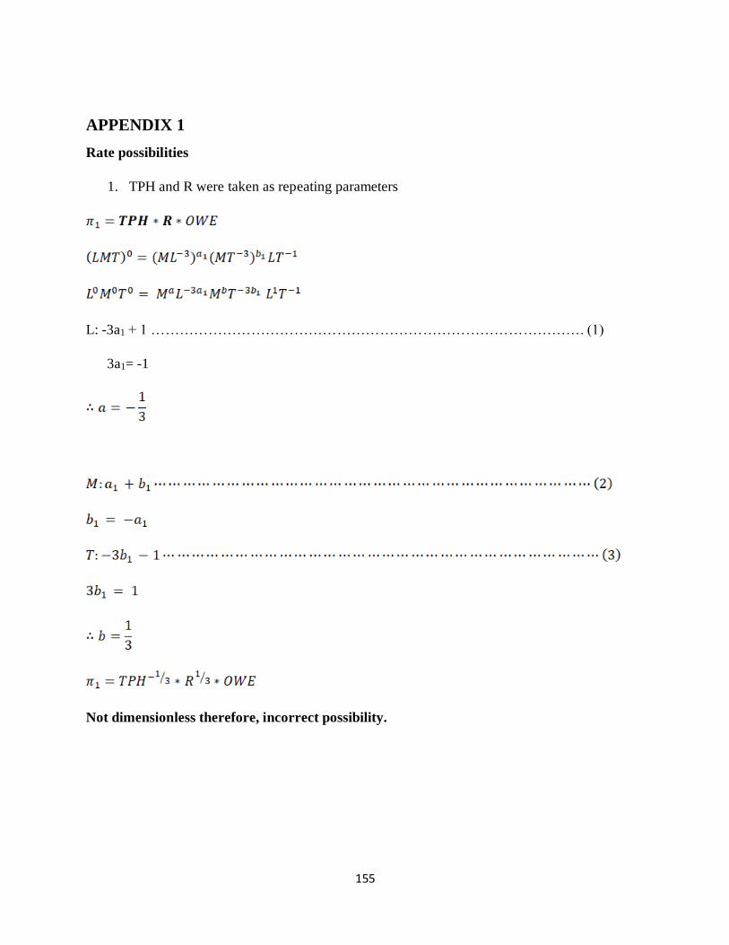
155
APPENDIX 1
Rate possibilities
1. TPH and R were taken as repeating parameters
L: -3a1 + 1 ………………………………………………………………………………. (1)
3a1= -1
Not dimensionless therefore, incorrect possibility.

Appendix: 1
156
Accumulation possibilities
2. TPH and R were taken as repeating parameters
L: -3a1 + 1 ………………………………………………………………………………. (1)
3a1= -1
Substitute a value into equation 2
Not dimensionless therefore, incorrect possibility

Appendix: 1
157
3. TSS, W and EC were taken as repeating parameters
L: -3a + b + 1 ……………………………………………………………………………. (1)
M: a + 0 a = 0 ………………………………………………………………………. (2)
T: -b -c b = -c …………………...……………………………………………… (3)
Substituting equation 2 into equation 1
-3(0) + b + 1 = 0
b = -1
Substituting b value into equation 3
-c = -1
c = 1

Appendix: 1
158
L: -3a2 + b2 + 1 …………………………………………………………………………. (1)
M: a2 + 0 a = 0 ………………………………………………………………………. (2)
T: -b2 -c2 b = -c2 …………………...……………………………………………… (3)
Substituting equation 2 into equation 1
-3(0) + b2 + 1 = 0
b2 = -1
Substituting b value into equation 3
-c2 = -1
c2 = 1
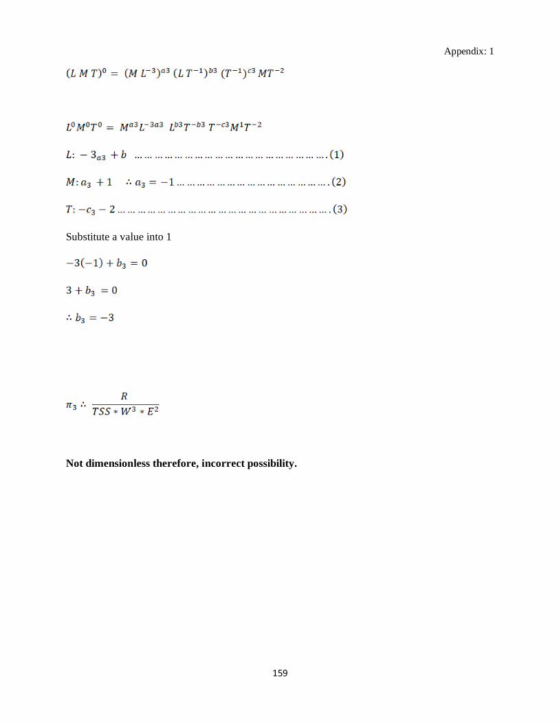
Appendix: 1
159
Substitute a value into 1
Not dimensionless therefore, incorrect possibility.

Appendix: 1
160
4. W, R and TSS were chosen as the repeating parameters:
L: a – 3c + 1 ………………………………………………………………………………. (1)
M: b + c b = - c …………………………………………. (2)
T: -a – 2b a = -2b …………………………………………. (3)
Substitute equations 2 and 3 into equation 1
b = -1
Substitute b value into equation 3.
a = -2(-1) = 2
∴
L: a2 -3c2 + 1 …………………………………………………………………………. (1)
M: b2 + c2 ……………………………………………………………………………… (2)
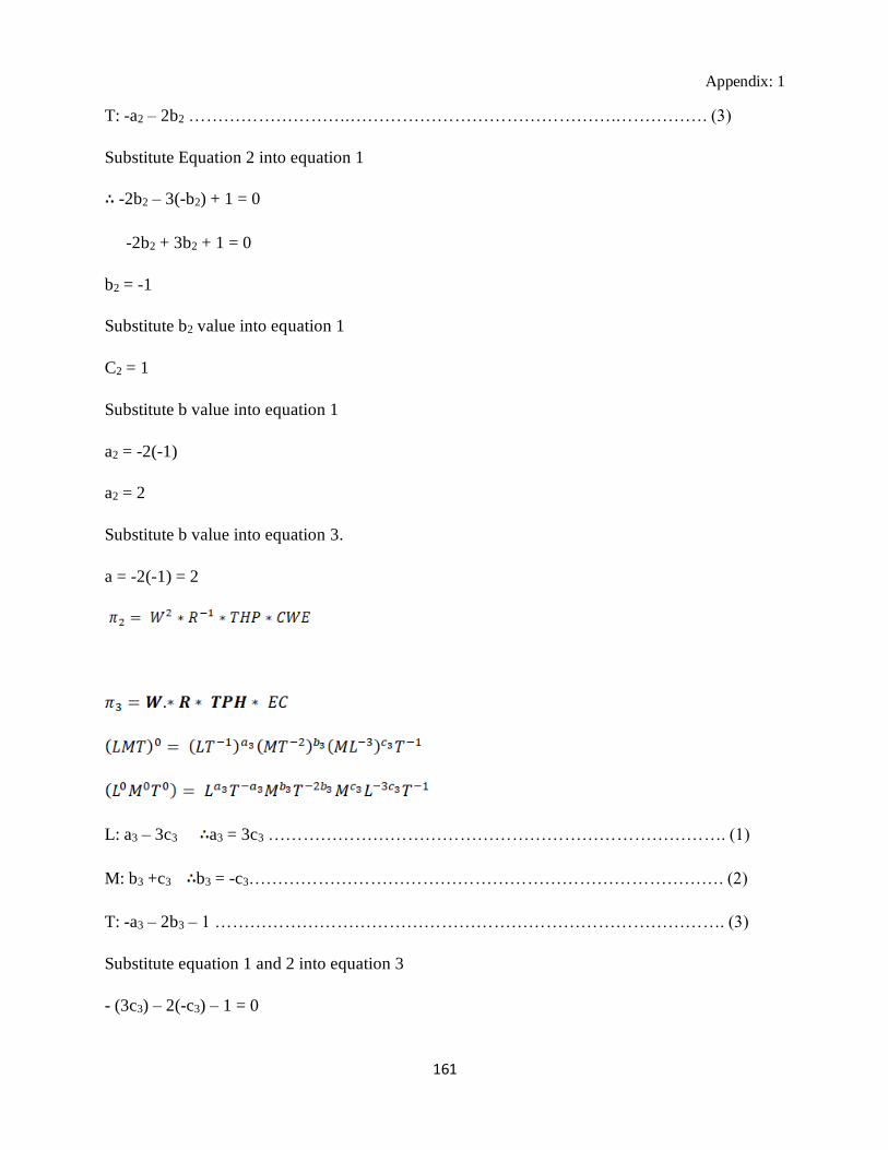
Appendix: 1
161
T: -a2 – 2b2 ……………………….……………………………………….……………. (3)
Substitute Equation 2 into equation 1
-2b2 – 3(-b2) + 1 = 0
-2b2 + 3b2 + 1 = 0
b2 = -1
Substitute b2 value into equation 1
C2 = 1
Substitute b value into equation 1
a2 = -2(-1)
a2 = 2
Substitute b value into equation 3.
a = -2(-1) = 2
L: a3 – 3c3 a3 = 3c3 ……………………………………………………………………. (1)
M: b3 +c3 b3 = -c3………………………………………………………………………. (2)
T: -a3 – 2b3 – 1 ……………………………………………………………………………. (3)
Substitute equation 1 and 2 into equation 3
- (3c3) – 2(-c3) – 1 = 0

Appendix: 1
162
-3c3 + 2c3 – 1 = 0
-c3 -1 = 0 c3 = -1
Substitute c value into equation 2……. ALSO …substitute c into equation 1
b3 + c3 = 0 a3 – 3c3 = 0
a3 = 3c3
b3 -1 = 0 a3 = 3(-1)
b3 = 1 a3 = -3
L: a4 -3c4 – 3 ………………………………………………………………………………. (1)
M: b4 + c4 + 1 c4 = -b4 – 1 ………………………. (2)
T: -a – 2b a4 = -2b4 ……………….…………. (3)
Substitute equations 2 and 3 into equation 1
-2b4 – 3 (-b4 – 1) – 3 = 0
-2b4 + 3b4 + 3 – 3 = 0
b4 = 0
Substitute b value into equation 3

Appendix: 1
163
-a4 = -2b4
a4 = 0
Substitute b value into equation 2
c4 = -b4 – 1
c4 = 0 – 1
c = -1
L: a5 – 3c5 – 3 ………………………………………………………………………… (1)
M: b5 + c5 + 1; c = -b5 – 1 ……….……………………. (2)
T: -a5 -2b5; a = -2b5 ………..……………………… (3)
Substitute equations 2 and 3 into equation 1
-2b5 - 3(-b5 – 1) – 3 = 0
-2b5 + 3b5 + 3 – 3 = 0
b5 = 0
Substitute b value into equation 3

Appendix: 1
164
a= = -2b
a5 = 0
Substitute b value into equation 2
c5 = -b – 1
c5 = 0 – 1
c5 = -1
After solving the pi terms. A general formula will be obtained:
Following dimensional analysis based on Buckingham pi theorem:

Appendix: 1
165
Incorrect possibility, according to Buckingham π theorem each parameter should be used
once.

Appendix: 1
166