development of a gestural master interface for tele ... · manipular o valor da sua 3º junta...
TRANSCRIPT

Development of a Gestural Master Interface for Tele-Surgery
Applications
Sérgio Miguel Saraiva Afonso
Thesis to obtain the Master of Science Degree in
Mechanical Engineering
Supervisor: Prof. Jorge Manuel Mateus Martins
Examination Committee
Chairperson: João Rogério Caldas Pinto
Supervisor: Prof. Jorge Manuel Mateus Martins Member of the Committee: João Carlos Prata dos Reis
November 2014


Twenty years from now you will be more disappointed by the things that you didn’t do than by the
ones you did do, so throw off the bowlines, sail away from safe harbor, catch the trade winds in
your sails. Explore, Dream, Discover.
Mark Twain


iii
Acknowledgments
First of all, I would like to acknowledge my supervisor, Prof. Jorge Martins, who guided me through this
work, providing me knowledge, suggestions and invaluable feedback that made this thesis possible.
To my parents and sister, for all their patience, comprehension, support and love since the beginning.
Without them this degree would never be possible.
To all my friends and classmates, but especially to Diogo Sampaio, Gonçalo Saraiva and Tomás Lúcio for
being present in all the moments of my journey in the IST, making this degree an unforgettable experience.
To my friends and colleagues at the laboratory: Claudio Brito, João Ramalhinho, Pedro Teodoro and Walter
Veiga for the shared moments of leisure and knowledge.
To my friends Nuno Correia, André Deodado, André Marques and Tiago Caeiro for all the support during
these 5 years.
To all the staff of the Medical Robotics Laboratory for their kindness.
And last, but not least, to Inês for all her love, patience, support and confidence.

v
Abstract
The present work focus in the implementation of a virtual surgical environment to perform Minimally Invasive
Robotic Surgery (MIRS), using as slaves the manipulators KUKA LWR IV and the EndoWrist® instruments
from the Da Vinci® Surgical System. Since the master’s controls of the da Vinci® system don’t provide any
force feedback, it’s introduced in this thesis an alternative where the actual robotic master system is
replaced by a new gestural interface. This new master doesn’t require any robotic equipment since it uses
the Leap Motion® (LM), which is a gesture-based interface, to recognize the motions of the surgeon’s hands,
wrists and fingers and translate them intro precise instruments’ movements. Therefore, it’s desired to detect
and surpass the imperfections and/or limitations in the kinematics of the manipulators and evaluate the
performance of the LM in MIRS as a gestural master interface.
The derived kinematic models presented good results with small tracking errors. Also, with the use of the
Closed-Loop Inverse Kinematics to solve the inverse kinematics, the redundancy of the manipulator KUKA
was used to avoid its own joint limits and to manipulate the value of the KUKAs’ 3rd joint without producing
any movement at the manipulators’ end-effector. The algorithm Remote Center of Motion was successfully
used to allow the instruments’ motion at the trocar point without injuring the patient. Finally, the results
showed that the model’s performance was fairly decreased by the LM’s limitations, more specifically, the
performance of the instrument’s yaw and roll motion.
Keywords
Minimally Invasive Robotic Surgery, Leap Motion, Remote Center of Motion, Closed-Loop Inverse
Kinematics, Gestural master interface, KUKA LWR IV


vii
Resumo
O presente trabalho tem como foco a implementação de um ambiente cirúrgico virtual para realizar Cirurgia
Robótica Minimamente Invasiva, usando, como escravos, os manipuladores KUKA LWR IV e os
instrumentos EndoWrist® do sistema cirúrgico da Vinci®. Visto que o mestre do sistema da Vinci® não
fornece qualquer feedback, é introduzida nesta tese uma nova alternativa onde o atual sistema mestre
robótico é substituído por uma nova interface gestual. Este novo mestre não necessita de nenhum
equipamento robótico, pois utiliza o Leap Motion® (LM), que se trata de uma interface baseada em gestos,
para reconhecer os movimentos das mãos, punhos e dedos do cirurgião e traduzi-los em precisos
movimentos dos instrumentos. Desta forma, é pretendido detetar e superar as limitações na cinemática
dos manipuladores e avaliar o desempenho do LM para ser utilizado como mestre.
Os modelos cinemáticos derivados apresentaram bons resultados com erros de seguimento pequenos.
Além disso, com a utilização do Closed-Loop Inverse Kinematics para resolver a cinemática inversa, a
redundância do manipulador KUKA foi utilizada para evitar atingir os seus próprios limites de junta e para
manipular o valor da sua 3º junta através do espaço nulo do jacobiano. O Centro Geométrico de Rotação
foi também utilizado com sucesso para permitir o movimento dos instrumentos no ponto de incisão sem
lesar o paciente. Finalmente, os resultados mostram que as limitações do LM reduziram bastante a
performance do modelo, mais especificamente, os movimentos yaw e roll do instrumento.
Palavras-Chave
Cirurgia Robótica Minimamente Invasiva, Leap Motion, Centro Geométrico de Rotação, Closed-Loop
Inverse Kinematics, Interface gestual como mestre, KUKA LWR IV

ix
Contents
Acknowledgments ....................................................................................................................................... iii
Abstract ......................................................................................................................................................... v
Resumo........................................................................................................................................................ vii
Contents ....................................................................................................................................................... ix
List of Figures .............................................................................................................................................. xi
List of Tables .............................................................................................................................................. xv
List of Acronyms ...................................................................................................................................... xvii
List of Symbols .......................................................................................................................................... xix
1. Introduction .......................................................................................................................................... 1
1.1 Minimally Invasive Surgery ............................................................................................................ 1
1.2 Minimally Invasive Robotic Surgery .............................................................................................. 2
1.3 State of The Art ............................................................................................................................. 4
1.3.1 da Vinci® Surgical System ..................................................................................................... 5
1.3.2 Leap Motion® ......................................................................................................................... 8
1.3.3 KUKA-DLR Lightweight Robot IV ........................................................................................ 10
1.4 Thesis Scope ............................................................................................................................... 12
1.5 Main Results ................................................................................................................................ 13
1.6 Thesis Outline .............................................................................................................................. 14
2. Description of the Leap Motion® software ...................................................................................... 17
2.1 Leap Motion® v1 .......................................................................................................................... 17
2.1.1 LM Architecture.................................................................................................................... 17
2.1.2 API Overview ....................................................................................................................... 18
2.1.3 An overview on the SDK and frame data ............................................................................ 20
2.1.4 Limitations of the Leap Motion® v1 ...................................................................................... 22
2.2 Leap Motion® v2 .......................................................................................................................... 24
2.3 Leap Motion® v1 vs Leap Motion® v2 .......................................................................................... 26
3. The interface between Leap Motion® SDK and MATLAB® ............................................................. 27
3.1 Matleap: The connection between Leap Motion® and MATLAB®................................................ 27
3.2 MATLAB® hand’s model .............................................................................................................. 29
4. Kinematics of Robotic Manipulators ............................................................................................... 37
4.1 Kinematics of the EndoWrist® instruments ................................................................................. 37

x
4.1.1 Direct Kinematics ................................................................................................................. 38
4.1.2 Inverse Kinematics .............................................................................................................. 40
4.2 Kinematics of the manipulator KUKA LWR IV ............................................................................. 44
4.2.1 Direct Kinematics ................................................................................................................. 44
4.2.2 Inverse Kinematics .............................................................................................................. 45
5. Implementation of the model - KUKA LWR IV + EndoWrist® instruments .................................. 49
5.1 Solver parameters ....................................................................................................................... 50
5.2 Data acquisition ........................................................................................................................... 50
5.3 CLIKs ........................................................................................................................................... 51
5.3.1 Coordinate Transformations: Pre-Instruments .................................................................... 52
5.3.2 Instrument’s CLIK and KUKA’s CLIK................................................................................... 53
5.3.3 RCM Algorithm .................................................................................................................... 54
5.4 Footswitches’ control ................................................................................................................... 55
5.5 Simulink® model – VRML ............................................................................................................ 55
5.6 Master Console ........................................................................................................................... 57
6. Experimental Results ........................................................................................................................ 59
6.1 Validation of the Kinematics ........................................................................................................ 59
6.2 Validation of the RCM Algorithm ................................................................................................. 64
6.3 Validation of the Hands’ Movements ........................................................................................... 70
7. Conclusions and Further Work ........................................................................................................ 75
7.1 Further Work ................................................................................................................................ 76
References ................................................................................................................................................. 79
Appendix .................................................................................................................................................... 83
Appendix A: Leap Motion® Control Panel ................................................................................................ 85
Appendix B: Auxiliary Functions to Build The Hand's Model .................................................................. 87
Appendix C: Implemented model ............................................................................................................ 91

xi
List of Figures
Figure 1.1 - MIS setup. ................................................................................................................................. 1
Figure 1.2 - Tele-operated Minimally Invasive Surgery (adapted from [14]) ................................................ 4
Figure 1.3 - OR Setup General [18] .............................................................................................................. 5
Figure 1.4 - Surgeon’s console: A – stereo viewer; B – surgeon touchpad and fingertip controls; C –
footswitch panel ............................................................................................................................................. 6
Figure 1.5 (b) - EndoWrist® instrument shell ................................................................................................ 7
Figure 1.6 ...................................................................................................................................................... 7
Figure 1.7 - Leap Motion® assembly ............................................................................................................ 8
Figure 1.8 - Leap Motion® schematic (adapted from [22]) ............................................................................ 9
Figure 1.9 - Leap Motion's® Field Of View .................................................................................................. 10
Figure 1.10 - KUKA Lightweight Robot [34] ................................................................................................ 11
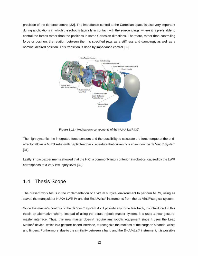
Figure 1.11 - Mechatronic components of the KUKA LWR [32] ................................................................. 12
Figure 2.1 - Native Application Interface .................................................................................................... 18
Figure 2.2 - LM Visualizer ........................................................................................................................... 18
Figure 2.3 - The LM coordinate system (adapted from [24]) ...................................................................... 19
Figure 2.4 - In red Fingers (left) and Tool detected (right) [24] .................................................................. 19
Figure 2.5 - LM recognized gestures [24] ................................................................................................... 20
Figure 2.6 - Hierarchy of the classes which constitute a frame .................................................................. 22
Figure 2.7 - Limitations on the rotation of the hand –rotation to the right NOT OK (image number 1 and 2);
rotation to the left OK (image number 3 and 4) ........................................................................................... 23
Figure 2.8 - Fingers lost when the hand is perpendicular to the device ..................................................... 23
Figure 2.9 - Despite being two hands in the field of view of the LM, only one hand is detected ................ 23
Figure 2.10 - When two fingers touch each other, the LM transforms them in only one finger .................. 23
Figure 2.11 - Hand stability ......................................................................................................................... 24
Figure 2.12 - Pinch Strength ....................................................................................................................... 24
Figure 2.13 - Bone type .............................................................................................................................. 25
Figure 2.14 - Data confidance .................................................................................................................... 25
Figure 2.15 - Hierarchy of the classes which constitute a frame (v2) [40] ................................................. 25
Figure 2.16 - v2 can’t hide the 3 rightmost fingers ..................................................................................... 26
Figure 2.17 - v1 with 3 fingers hidden ........................................................................................................ 26
xii
Figure 3.1 - EndoWrist® instrument (left) hand and fingers detected by the LM (center) and user’s hand
(right) at the same configuration. ................................................................................................................. 30
Figure 3.2 - Configurations not supported: top images (more than 2 hands or more than 2 fingers in each
hand). Configuration supported: bottom image (2 fingers in each hand). ................................................... 31
Figure 3.3 - Classification of the pointables: 1-right indicator, 2-right thumb, 3-left thumb and 4-left
indicator. ...................................................................................................................................................... 32
Figure 3.4 - Hand’s Classification ............................................................................................................... 33
Figure 3.5 - Hand’s attributes. .................................................................................................................... 33
Figure 3.6 - Hand with 5 fingers, a configuration accepted to control the camera. .................................. 34
Figure 3.7 - 2 hands with 9 fingers, a configuration accepted to control the KUKAs' null-space (section
5.3.2). ........................................................................................................................................................... 35
Figure 4.1 - Kinematic model ...................................................................................................................... 37
Figure 4.2 - DH kinematic parameters ........................................................................................................ 38
Figure 4.3 - Distribution of the coordinate axes (left) and EndoWrist® instrument (right) ........................... 40
Figure 4.4 - Closed-Loop Inverse Kinematics (adapted from [37]) ............................................................ 44
Figure 4.5 - KUKA LWR (left) and Distribution of the coordinate axes (right) ............................................ 45
Figure 4.6 - Closed-Loop Inverse Kinematics (adapted from [37]) ............................................................ 48
Figure 5.1 - Implemented model with CLIKs in series ................................................................................ 52
Figure 5.2 - Surgical Instrument’s DOFs .................................................................................................... 53
Figure 5.3 - KUKA (black), instrument (blue) and the position components to compute the RCM (adapted
from [41]) ..................................................................................................................................................... 54
Figure 5.4 - Virtual surgical environment – Top View ................................................................................. 56
Figure 5.5 - Virtual surgical environment – Robots + patient ..................................................................... 56
Figure 5.6 - Surgeon's Console .................................................................................................................. 57
Figure 6.1 - 𝑘 = 0.01: Reference (blue) vs CLIK result (red) ...................................................................... 60
Figure 6.2- k = 0.05: Reference (blue) vs CLIK result (red) ....................................................................... 60
Figure 6.3 - Reference (blue) vs CLIK result (red) without solving the redundancy ................................... 61
Figure 6.4 - Orientation error without solving the redundancy ................................................................... 61
Figure 6.5 - Position error without solving the redundancy ........................................................................ 61
Figure 6.6 - Joint angles without solving the redundancy .......................................................................... 62
Figure 6.7 - Reference (blue) vs CLIK result (red) ..................................................................................... 63
Figure 6.8 - Joint Angles ............................................................................................................................. 63
Figure 6.9 - Orientation error ...................................................................................................................... 63
Figure 6.10 - Position Error......................................................................................................................... 63
Figure 6.11 - Position error: displacement depending on the movements’ velocity ................................... 64
Figure 6.12 - Orientation error: comparison between different movements' velocities .............................. 65

xiii
Figure 6.13 - (LEFT) Position’s tracking error: Reference (blue) vs CLIK result (red); (RIGHT)
Orientation’s tracking error (normal component): Reference (blue) vs CLIK result (red) ........................... 66
Figure 6.14 - (LEFT) Orientation’s tracking error (slide component): Reference (blue) vs CLIK result (red);
(RIGHT) Orientation’s tracking error (approach component): Reference (blue) vs CLIK result (red) ......... 66
Figure 6.15 - (LEFT) Orientation error; (RIGTH) Position error .................................................................. 67
Figure 6.16 - Joint angles ........................................................................................................................... 67
Figure 6.17 - (LEFT) Position’s tracking error: Reference (blue) vs CLIK result (red); (RIGHT)
Orientation’s tracking error (normal component): Reference (blue) vs CLIK result (red) ........................... 68
Figure 6.18 - (LEFT) Orientation’s tracking error (slide component): Reference (blue) vs CLIK result (red);
(RIGHT) Orientation’s tracking error (approach component): Reference (blue) vs CLIK result (red) ......... 68
Figure 6.19 - (LEFT) Orientation error; (RIGTH) Position error .................................................................. 69
Figure 6.20 - Joint angles ........................................................................................................................... 69
Figure 6.21 - Limitations on the instrument's 4th DOF ................................................................................ 71
Figure 6.22 - Limitations on the instrument's 5th DOF ................................................................................ 71
Figure 6.23 - Motion of the instrument's 6th DOF ....................................................................................... 72
Figure 6.24 - Grasping motion .................................................................................................................... 72
Figure 6.25 - Interaction between the user's hands and the surgical instruments ..................................... 72
Figure 6.26 - Simulation to test the hand tremor ........................................................................................ 73
Figure A.1 - LM Control Panel .................................................................................................................... 85
Figure C.2 - Implemented model in Simulink® environment ....................................................................... 91


xv
List of Tables
Table 1.1: Advantages and Disadvantages of Robot-Assisted Surgery Versus Conventional Surgery
[10][11] ........................................................................................................................................................... 3
Table 3.1 - Similarity between the hand and the EndoWrist® instruments. ................................................ 30
Table 4.1 - DH parameters.......................................................................................................................... 40
Table 4.2 - DH parameters.......................................................................................................................... 45
Table 6.1 - Limits of the manipulator's joints ............................................................................................... 61
Table 6.2 - Hand tremor results .................................................................................................................. 73


xvii
List of Acronyms
MIS Minimally invasive surgery
MIRS Minimally invasive robotic surgery
LWR Lightweight Robot
DLR German Aerospace Center
LM Leap Motion®
API Application Programmer Interface
SDK Software Development Kit
DOF Degrees Of Freedom
CLIK Closed-Loop Inverse Kinematics
VRML Virtual Reality Modeling Language
LMC Leap Motion Controller
app Application
CPU Central processing unit
FOV Field Of View
RCM Remote Center of Motion
DH Denavit-Hartenber convention
DLS Damped Least-Squares
SM Simulink® model
L2S Leap2simulink.m
DSR Data Store Read
MIS Minimally invasive surgery
MIRS Minimally invasive robotic surgery
LWR Lightweight Robot
DLR German Aerospace Center
LM Leap Motion®
API Application Programmer Interface
SDK Software Development Kit
DOF Degrees Of Freedom


xix
List of Symbols
𝒙𝒆 End-effector position and orientation in Cartesian Space
𝑿 End-effector velocity in Cartesian Space
𝒑𝒆, �̇� End-effector position and linear velocity in Cartesian Space
∅𝒆, 𝒘 End-effector orientation and angular velocity in Cartesian Space
𝒒, �̇� Joint angles positions and velocities
𝒅𝒊, 𝒗𝒊, 𝒂𝒊 ,𝜶𝒊 Denavit-Hartenber parameters
𝑻𝒊𝒊−𝟏 Homogeneous transformation matrix
𝑹𝒆 End-effector’s rotation matrix
𝑱 Geometric Jacobian
𝑱∗ Damped least-squares inverse
𝑸 Unit Quaternion
𝜼, 𝝐 Scalar part and Vector part of a quaternion
𝑺(∙) Skew-symmetric operator
𝒆𝑶,𝑸𝒖𝒂𝒕, 𝒆𝑷 End-effector’s orientation and position error in Cartesian Space
𝑲𝑷,𝑲𝑶 Position and orientation positive definite matrix
𝑱† Moore-Penrose Right Pseudo-Inverse
𝑵(𝑱(𝒒)) Null-space matrix
𝒒�̇� Joint velocities of the null-space
𝒘(𝒒) Objective function
𝒒𝒊𝑴, 𝒒𝒊𝒎 Maximum and minimum joint limits
�̅�𝒊 Middle value of the joint range
𝒃 Distance between trocar and KUKA’s end-effector
𝑳 Instruments length
𝒑𝑲𝑼𝑲𝑨 Position of the KUKA’s end-effector
𝒑𝒕𝒓𝒐𝒄𝒂𝒓 Trocar position
�⃗⃗� Normal relative to the instrument
𝑹𝟐𝟎 Orientation matrix from the frame 0 to the frame 2 of the surgical instrument
𝑹𝒐𝒕 Orientation matrix of the KUKA’s end-effector at its initial configuration

1
Chapter 1
1. Introduction
1.1 Minimally Invasive Surgery
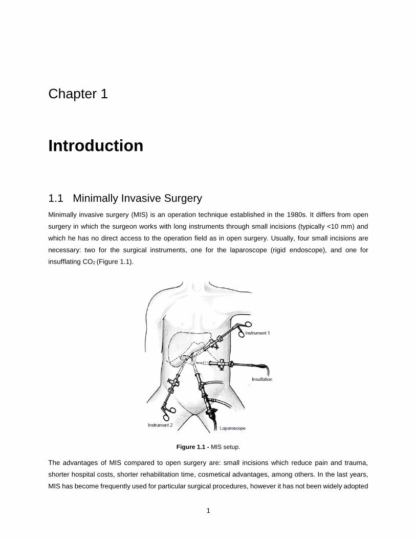
Minimally invasive surgery (MIS) is an operation technique established in the 1980s. It differs from open
surgery in which the surgeon works with long instruments through small incisions (typically <10 mm) and
which he has no direct access to the operation field as in open surgery. Usually, four small incisions are
necessary: two for the surgical instruments, one for the laparoscope (rigid endoscope), and one for
insufflating CO2 (Figure 1.1).
Figure 1.1 - MIS setup.
The advantages of MIS compared to open surgery are: small incisions which reduce pain and trauma,
shorter hospital costs, shorter rehabilitation time, cosmetical advantages, among others. In the last years,
MIS has become frequently used for particular surgical procedures, however it has not been widely adopted

2
for more complex or delicate procedures – for example mitral valve repair. This is due to the fact that, for
more complex procedures, the manipulation of fine-tissue is more difficult than in open surgery.
Of course, MIS has disadvantages as well. The use of a laparoscope requires the surgeon to manage the
instrument with reduced sight, which can lead to severe orientation problems during surgery. In a
conventional MIS the surgeon is required to view what it’s operating through a monitor that provides 2-D
vision, which leads to change the normal hand-eye target axis. Also, the 2-D vision doesn’t provide a full
stereoscopic depth perception. Furthermore, the camera used in MIS is held by an assistant, due to this the
surgeon doesn’t has control of the camera which causes an unsteady field of vision. An important point is
that the instruments have to be moved around an invariant point (trocar point) on the patient’s chest or
abdominal wall and as a result, reverse hand motion occurs as well as the amplification of the surgeon's
tremor. Also, the friction in the trocar reduces haptic feedback. The tissue’s palpation is also not possible,
since the surgeon does not have direct access to the operating area. The loss of haptic feedback may be
compensated by visual feedback, e.g. tissue deformation can be interpreted as a measure of the exerted
force. Yet, this does not work with stiff materials such as needles. Additionally, the surgeon's dexterity, when
performing certain tasks, is reduced dramatically. Therefore, the surgeon cannot reach any point in the
workspace at an arbitrary orientation. This represents a big drawback in MIS since for complex tasks, like
knot tying, it consumes a big amount of time and requires intensive training [1][2][3][4][5].
1.2 Minimally Invasive Robotic Surgery
During the last years several surgery robots developed at research institutes have entered hospitals for
experimental or even routine applications. Robodoc® from Integrated Surgical Systems Inc. [6] or Caspar®
from URS Universal Robot Systems [7] are used for bone surgery, whereas the Da Vinci® system from
Intuitive Surgery Inc. [8] or Zeus® from Computer Motion Inc. [9] have been designed for minimally invasive
surgery.
To avoid the drawbacks of manual MIS, minimally invasive robotic surgery (MIRS) plays an important role.
MIRS systems help the surgeon to overcome barriers which separates him from the operating area.
Furthermore, it is possible to overcome distances, like if surgeon and patient are located in different rooms
or even hospitals [5]. Also, the numbers of clinical applications increased due to the expected advantages
such as high precision, use of preoperative planning data and the possibility of new surgery techniques,
such as minimally invasive beating heart surgery. Nevertheless, robotic surgery still has some
disadvantages. Table 1.1 enumerates some Advantages and Disadvantages of Robot-Assisted Surgery
Versus Conventional Surgery.

3
Human strengths Human limitations Robot strengths Robot limitations
Strong hand–eye coordination
Dexterous
Flexible and adaptable
Can integrate extensive and diverse information
Rudimentary haptic abilities
Able to use qualitative information
Good judgment
Easy to instruct and debrief
Limited dexterity outside natural scale
Prone to tremor and fatigue
Limited geometric accuracy
Limited ability to use quantitative information
Limited sterility
Susceptible to radiation and infection
Good geometric accuracy
Stable and untiring
Scale motion
Can use diverse sensors in control
May be sterilized
Resistant to radiation and infection
No judgment
Unable to use qualitative information
Absence of haptic sensation
Expensive
Technology in flux
More studies needed
Table 1.1: Advantages and Disadvantages of Robot-Assisted Surgery Versus Conventional Surgery [10][11]
Many studies were performed in order to discover the feasibility of this robot-assisted surgery. For example,
one study done by Cadiere et al [12], evaluated the feasibility of robotic laparoscopic surgery on 146
patients, using the da Vinci® Surgical System. This study found that robotic laparoscopic surgery is feasible.
They also found the robot to be most useful in intra-abdominal microsurgery or for manipulations in very
small spaces .
Once introduced the MIRS with its advantages and disadvantages, it’s important to do an overview of the
system. The system consists in: surgeon side devices and patient side devices. The communication
between devices has to be flexible to allow the connection of different master stations (not necessarily
located in the same OR), to get support by an additional expert (which is today limited to video conferencing)
or to enhance training of surgeons. Therefore, the communication network has to be safe (guaranteed
bandwidth and no communication delay) and secure (no undesired third-party listening) [13].
Regarding the surgeon side devices, the surgeon maneuvers a master manipulator as an input device,
where the input data is transmitted to the patient side devices. As a consequence, the slave manipulators
move accordingly to the motion of the surgeon’s hands. Images from the endoscope and the motion of the
assistant and slave manipulators are shown in the surgeon side devices. The image of the surgeon is also
transmitted and presented at the patient side. The applied force to the forceps at the patient side, is
presented to the surgeon to provide a better user interface. The movements performed by the surgeon in
the master manipulator are transformed in position and orientation information and then are transmitted to
the slave. The master consists in left and right manipulator, where each manipulator has 7 degrees of
freedom - 3 translational, 3 rotational and 1 to control the grasp. If desired, the orientation of the tip of the
master manipulator is preserved at the same posture during the translational motion. Two footswitches are

4
provided in order to control the flow of data from the master to the slave. For example, if the disengage
pedal is pressed, the slaves will not move even if the master manipulators are being operated. Scaling the
surgeon's motion and filtering the surgeon's tremor are two additional important features to increase the
safety and accuracy of a MIRS system [13].
For the patient side devices, as it was said before, the slave moves accordingly to the surgeon movements.
The slave manipulators consist in 3 arms: 2 of them to hold forceps and the other one holds an endoscope.
The minimally invasive instruments should be small (diameter less than 10 mm) in order to reduce pain and
trauma to a minimum and should allow the measurement of force and tactile information. Additionally, the
instruments have to be very light so that they can be handled by one person easily (this is very important in
case of emergency situations, when the robots have to be removed to get direct access to the patient). In
order to ensure safety and rigidity of the system, radius guides are adopted to force the trocar position to
be at a fixed position by making it coincide with the rotational center of the radius guide – geometric center
of rotation. The system has also a degree of freedom to move all 3 arms at the same time in order to
determine the insertion position of the endoscope [13].
Figure 1.2 - Tele-operated Minimally Invasive Surgery (adapted from [14])
1.3 State of The Art
In this section, the da Vinci® Surgical System and its main features will be presented (1.3.1). Then, the Leap
Motion® software will be briefly introduced in order to explain how it works and presents its currents features.
An analysis of its performance is also made (1.3.2). Finally, it is presented the main features of the
manipulator KUKA Lightweight Robot (LWR) IV (1.3.3).

5
1.3.1 da Vinci® Surgical System
The da Vinci® Surgery System was approved by the FDA in mid-2000 for general laparoscopic surgery and
in the end of the year 2002 for mitral valve repair surgery. Until now different da Vinci® models have been
introduced such as the standard, streamlined (S), S-high definition (HD), the S integrated (i) and lastly the
fourth generation (Xi). Presently, this robot is used in various fields such as urology, general surgery, cardio-
thoracic, etc. Compared with the conventional surgery, it provides several advantages like 3D vision, motion
scaling, tremor filtration, etc [15].
This system consists of an ergonomically designed surgeon's console, a patient cart with four interactive
robotic arms, a high-performance vision system and a wide variety of patented EndoWrist® instruments
(Figure 1.3).
Figure 1.3 - OR Setup General [18]
This system requires the following surgical team: surgeon, circulating nurse, surgical technician and surgical
assistant(s). It promotes a less invasive technique than the traditional surgery and other MIRS, and today it
is the most successful system and the most commonly used in MIRS [11][16]. With this surgery the cuts
(incisions) made in the body by the surgeon are much smaller than the cuts made in MIS. Like it was said
previously, this type of surgery is better than the traditional surgery because it provides a shorter hospital
stay, less blood loss, fewer complications, a faster recovery and smaller incisions for minimal scarring [17].
6
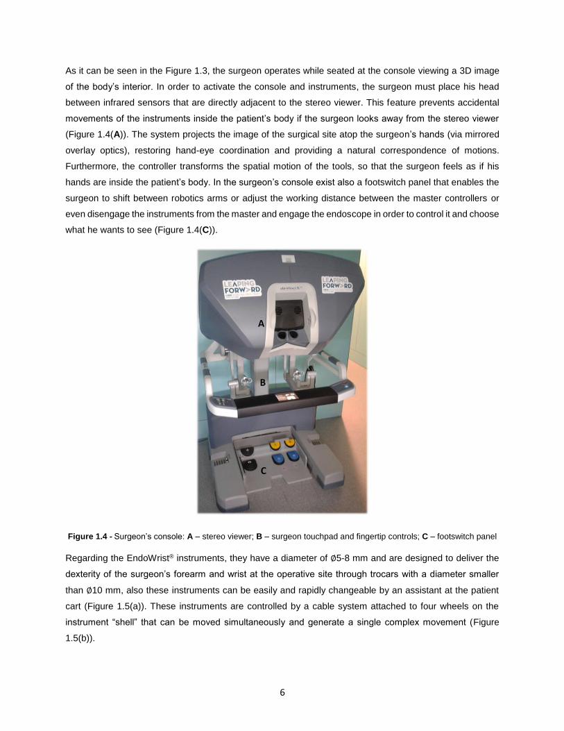
As it can be seen in the Figure 1.3, the surgeon operates while seated at the console viewing a 3D image
of the body’s interior. In order to activate the console and instruments, the surgeon must place his head
between infrared sensors that are directly adjacent to the stereo viewer. This feature prevents accidental
movements of the instruments inside the patient’s body if the surgeon looks away from the stereo viewer
(Figure 1.4(A)). The system projects the image of the surgical site atop the surgeon’s hands (via mirrored
overlay optics), restoring hand-eye coordination and providing a natural correspondence of motions.
Furthermore, the controller transforms the spatial motion of the tools, so that the surgeon feels as if his
hands are inside the patient’s body. In the surgeon’s console exist also a footswitch panel that enables the
surgeon to shift between robotics arms or adjust the working distance between the master controllers or
even disengage the instruments from the master and engage the endoscope in order to control it and choose
what he wants to see (Figure 1.4(C)).
Figure 1.4 - Surgeon’s console: A – stereo viewer; B – surgeon touchpad and fingertip controls; C – footswitch panel
Regarding the EndoWrist® instruments, they have a diameter of ∅5-8 mm and are designed to deliver the
dexterity of the surgeon’s forearm and wrist at the operative site through trocars with a diameter smaller
than ∅10 mm, also these instruments can be easily and rapidly changeable by an assistant at the patient
cart (Figure 1.5(a)). These instruments are controlled by a cable system attached to four wheels on the
instrument “shell” that can be moved simultaneously and generate a single complex movement (Figure
1.5(b)).
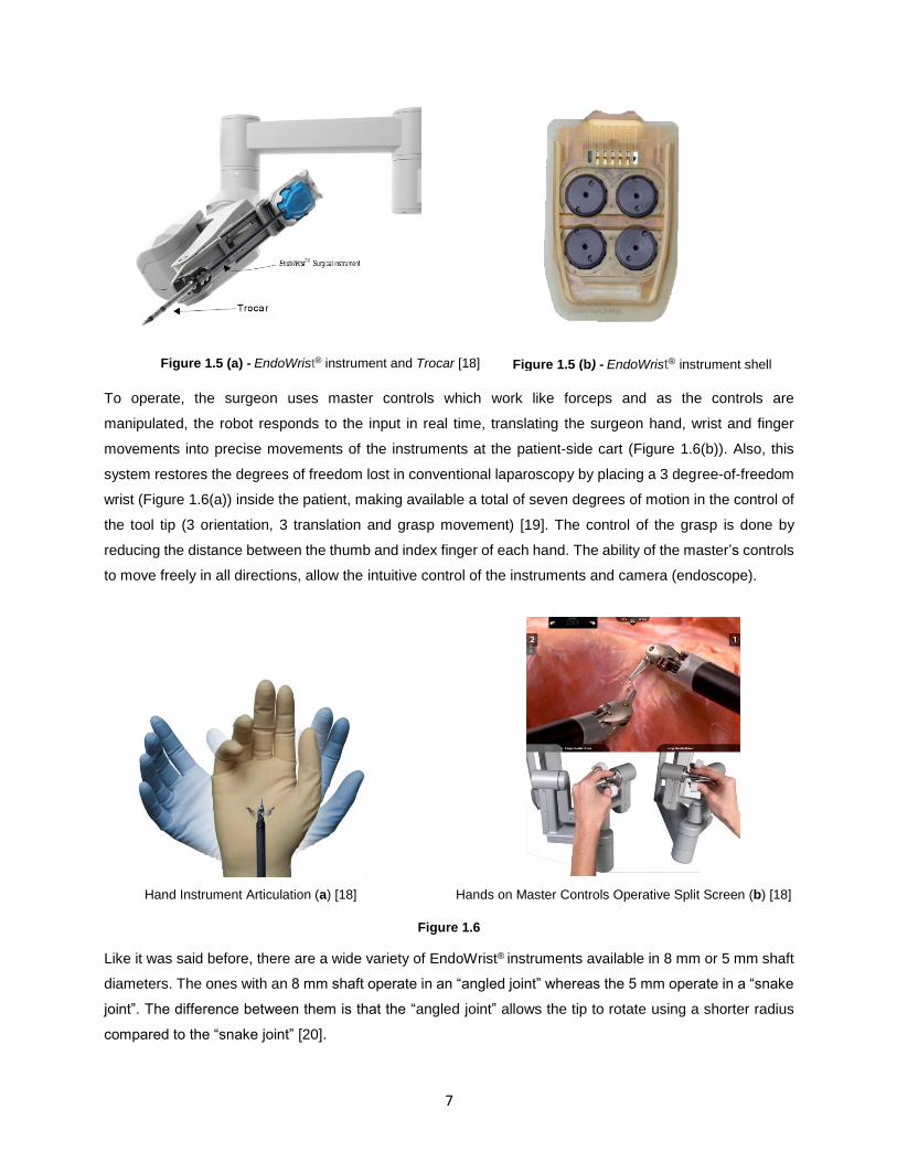
7
To operate, the surgeon uses master controls which work like forceps and as the controls are
manipulated, the robot responds to the input in real time, translating the surgeon hand, wrist and finger
movements into precise movements of the instruments at the patient-side cart (Figure 1.6(b)). Also, this
system restores the degrees of freedom lost in conventional laparoscopy by placing a 3 degree-of-freedom
wrist (Figure 1.6(a)) inside the patient, making available a total of seven degrees of motion in the control of
the tool tip (3 orientation, 3 translation and grasp movement) [19]. The control of the grasp is done by
reducing the distance between the thumb and index finger of each hand. The ability of the master’s controls
to move freely in all directions, allow the intuitive control of the instruments and camera (endoscope).
Hand Instrument Articulation (a) [18] Hands on Master Controls Operative Split Screen (b) [18]
Figure 1.6
Like it was said before, there are a wide variety of EndoWrist® instruments available in 8 mm or 5 mm shaft
diameters. The ones with an 8 mm shaft operate in an “angled joint” whereas the 5 mm operate in a “snake
joint”. The difference between them is that the “angled joint” allows the tip to rotate using a shorter radius
compared to the “snake joint” [20].
Figure 1.5 (a) - EndoWrist® instrument and Trocar [18] Figure 1.5 (b) - EndoWrist® instrument shell
8
Lastly, with the use of this technology the surgeon’s hand movements are more accurate, the surgeon’s
tremors are filtered and amplitude’s movement is scaled, which ensures that the instruments’ tip remain
more steadier than in the conventional MIS [16].
The good performance of the da Vinci® robot can be found in “Casos Clínicos Hospital da Luz 2012-2013”.
In this book, it is described a clinical case where it was performed the reconstruction of the normal anatomy
(by laparoscopic) and a duodenal switch (by the da Vinci® robot) in a patient [28]. The reason by which the
reconstruction of the normal anatomy was performed by laparoscopy is due to the fact that it was performed
in multi quadrants. To use the robot it would be necessary to constantly move its position and the patient
position, which would make the process tiresome and unpractical. Regarding the use of the robot to perform
the duodenal switch, the high precision in the dissection, the high dexterity of the instruments and the high
definition of the three-dimensional vision facilitated the work of the surgeon. Also, the constraints imposed
by the abdominal wall were supported by the patient cart (Figure 1.3). In conclusion, the use of this robot
allowed the surgery to be performed more safely and with greater comfort than in open surgery.
In this thesis the main focus will be in how to control the EndoWrist® instruments without using the existing
master console. This last point will be better explained in the section 1.4.
1.3.2 Leap Motion®
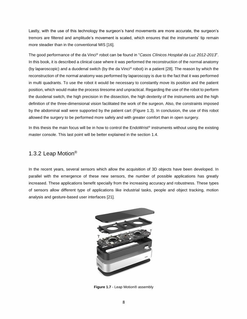
In the recent years, several sensors which allow the acquisition of 3D objects have been developed. In
parallel with the emergence of these new sensors, the number of possible applications has greatly
increased. These applications benefit specially from the increasing accuracy and robustness. These types
of sensors allow different type of applications like industrial tasks, people and object tracking, motion
analysis and gesture-based user interfaces [21].
Figure 1.7 - Leap Motion® assembly

9
With the creation of the Leap Motion® (LM) (Figure 1.7), a new gesture and position tracking system with
millimeter accuracy is achieved. This device uses a pair of cameras and an infrared pattern projected by
LEDs to generate an image of the user’s hands with depth information (Figure 1.8). Hence, the LM can be
categorized into optical tracking system based on Stereo Vision. The images acquired by the device are
post-processed in a computer in order to remove noise and construct a model of the hands, fingers, tools
and gestures [21].
This controller, together with the existing API (Application Programming Interface), provides positions in
Cartesian space of objects like finger tips and tool tips. The acquired positions are calculated relative to the
LM center point, which is located at the center of the device (Figure 1.8) [21]. In order to develop
applications, the LM Software Development Kit (SDK) is used since it contains the necessary libraries to
develop the project presented in this thesis.
Figure 1.8 - Leap Motion® schematic (adapted from [22])
Bearing in mind that the majority of applications for the LM controller are gesture-based, and due to the fact
that the tremor1 is always present in the human hand motion, the accuracy of this device when reading the
motion of a human hand is a very important factor. From Weichert et al. [21], the deviation between the
desired 3D position and the average measured positions was less than 0.2 mm for static setups and 1.2
mm for dynamic setups. The repeatability had an average of less than 0.17 mm. Although was not possible
to achieve the theoretical accuracy of 0.01 mm, this device achieved a high precision when compared with
other gesture-based interfaces (e.g. Microsoft Kinect®).
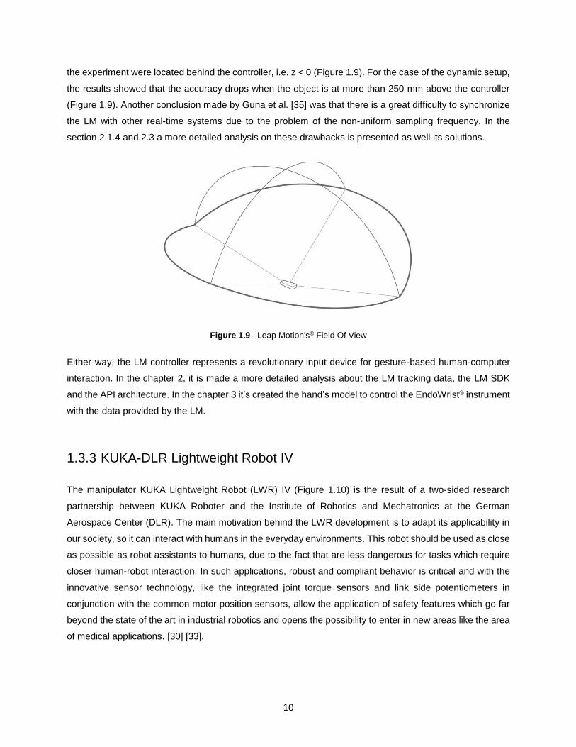
Another evaluation was performed by Guna et al. [35], where the main goal was to “analyze the controller’s
sensory space and to define the spatial dependency of its accuracy and reliability”. For the static setup, the
first results obtained a standard deviation of 0.5 mm and when combined with the high accuracy mentioned
before, the controller showed to be reliable and accurate to track static points. However, the standard
deviation revealed a significant increase when moving away from the controller, i.e. at the vicinity of the
limits of the controller’s field of view (Figure 1.9). Also, the majority of the successfully selected points for
1 The human tremor has an amplitude that varies between the 0.4 mm ± 0.2 mm.
10
the experiment were located behind the controller, i.e. z < 0 (Figure 1.9). For the case of the dynamic setup,
the results showed that the accuracy drops when the object is at more than 250 mm above the controller
(Figure 1.9). Another conclusion made by Guna et al. [35] was that there is a great difficulty to synchronize
the LM with other real-time systems due to the problem of the non-uniform sampling frequency. In the
section 2.1.4 and 2.3 a more detailed analysis on these drawbacks is presented as well its solutions.
Figure 1.9 - Leap Motion's® Field Of View
Either way, the LM controller represents a revolutionary input device for gesture-based human-computer
interaction. In the chapter 2, it is made a more detailed analysis about the LM tracking data, the LM SDK
and the API architecture. In the chapter 3 it’s created the hand’s model to control the EndoWrist® instrument
with the data provided by the LM.
1.3.3 KUKA-DLR Lightweight Robot IV
The manipulator KUKA Lightweight Robot (LWR) IV (Figure 1.10) is the result of a two-sided research
partnership between KUKA Roboter and the Institute of Robotics and Mechatronics at the German
Aerospace Center (DLR). The main motivation behind the LWR development is to adapt its applicability in
our society, so it can interact with humans in the everyday environments. This robot should be used as close
as possible as robot assistants to humans, due to the fact that are less dangerous for tasks which require
closer human-robot interaction. In such applications, robust and compliant behavior is critical and with the
innovative sensor technology, like the integrated joint torque sensors and link side potentiometers in
conjunction with the common motor position sensors, allow the application of safety features which go far
beyond the state of the art in industrial robotics and opens the possibility to enter in new areas like the area
of medical applications. [30] [33].

11
Figure 1.10 - KUKA Lightweight Robot [34]
This manipulator is similar to the human arm, i.e. 7 DOF, which allows the existence of redundancy which
can be used to reduce collision risk. Its main features are: load-to-weight ratio of 1:1, a total system weight
of less than 15kg, work space up to 1.5m, integrated force torque sensors in each joints which enables
compliant behavior without significantly loss of accuracy in the position, two position sensors per axis for
redundancy and safety reasons, active vibration damping and compliant control at joint and Cartesian level
[31]. The measurements are executed, in all joints, at a 3 kHz cycle, by means of:
Strain gauge-based torque-sensing;
Motor position sensing - based on magneto-resistive encoders;
Link-side position sensing - based on potentiometers - used as redundant sensors for safety
reasons.
Torque sensors are fixed at the flex spline component of the Harmonic Drive gear and measure the joint
torques acting on the joints. The error of these sensors is below 0.5%. In addition, the decoupling of the
disturbing forces and torques is also performed by means of a bearing. This high performance is only
achieved through the use of lightweight Harmonic Drive gears and RoboDrive motors possessing high
energy density [32].
In order to provide robust performance and safety for the human-robot interaction, the design of control laws
is a crucial step. Evaluating the torques in the joints is essential, since there is always a probability of
collision with its surroundings. To do so, a control at the joints level is performed by means of a decentralized
state feedback controller. This controller uses the entire joint state in the feedback loop, i.e. the position 𝜃
and the velocity �̇� of the motors and the joints torque 𝜏 and its derivative �̇�. The feedback terms have also
a very intuitive physical interpretations. First the torque feedback reduces the inertia of the motors and the
joint friction and secondly, the motor position feedback is equivalent to a physical spring and the velocity
feedback produces energy dissipation. Therefore, stability can be ensured in contact with any environment,
as long as it displays a passive behavior. An extra wrist force-torque sensor can be used to increase the
12
precision of the tip force control [32]. The impedance control at the Cartesian space is also very important
during applications in which the robot is typically in contact with the surroundings, where it is preferable to
control the forces rather than the positions in some Cartesian directions. Therefore, rather than controlling
force or position, the relation between them is specified (e.g. as a stiffness and damping), as well as a
nominal desired position. This transition is done by impedance control [32].
Figure 1.11 - Mechatronic components of the KUKA LWR [32]
The high dynamic, the integrated force sensors and the possibility to calculate the force torque at the end-
effector allows a MIRS setup with haptic feedback, a feature that currently is absent on the da Vinci® System
[31].
Lastly, impact experiments showed that the HIC, a commonly injury criterion in robotics, caused by the LWR
corresponds to a very low injury level [32].
1.4 Thesis Scope
The present work focus in the implementation of a virtual surgical environment to perform MIRS, using as
slaves the manipulator KUKA LWR IV and the EndoWrist® instruments from the da Vinci® surgical system.
Since the master’s controls of the da Vinci® system don’t provide any force feedback, it’s introduced in this
thesis an alternative where, instead of using the actual robotic master system, it is used a new gestural
master interface. Thus, this new master doesn’t require any robotic equipment since it uses the Leap
Motion® device, which is a gesture-based interface, to recognize the motions of the surgeon’s hands, wrists
and fingers. Furthermore, due to the similarity between a hand and the EndoWrist® instrument, it is possible
13
to create a hand’s model, from what it is detected by the Leap Motion®, to handle the instruments’ motion
intuitively. Therefore, it is intended to:
Analyze the potential of the LM in order to determine which are the limitations with the use of this
software to perform MIRS;
Construct the model of the hand from the data provided by the LM and use it as a gestural master
interface;
Derive two kinematical models, one for each manipulator, to control the manipulators in the
Cartesian Space;
Implement the tele-manipulation robot-surgeon model in a real-time dynamic virtual model;
Design a master console containing the LM device, two monitors, footswitches (to allow the control
of the camera’s viewpoint), a pc and a structure to support the user’s arms.
Also, with the implementation of the virtual model it’s desired to: detect and surpass the imperfections and/or
limitations in the kinematics of the manipulators; evaluate the performance of the Leap Motion® to recognize
the user’s hands motions to perform MIRS; and evaluate the robustness provided by the model to perform
MIRS.
1.5 Main Results
In this section are presented the main results obtained with the realization of this work.
First, the kinematical models, for both manipulators, presented good results since it was possible to move
the manipulators in the Cartesian space with a small tracking error (magnitude of 10−3). Also, the
implementation of the algorithm Closed-Loop Inverse Kinematics to solve the inverse kinematics, allowed
to use the redundancy of the manipulator KUKA to avoid its own joint limits and to use the null-space of the
Jacobian to manipulate the value of the KUKAs’ 3rd joint without producing any movement at the
manipulators’ end-effector.
The algorithm Remote Center of Motion, used to solve the constraint at the trocar point, showed also good
results since it allowed the instruments to move around and along the trocar point, without injuring the
surrounding tissues. Moreover, the implementation of this algorithm didn’t degrade the model, since the
maximum displacement of the instrument at the trocar point, for slow/moderate movements (< 2𝑚/𝑠), was
of 1 mm.
Regarding the limitations of the LM to detect certain hand poses, it was possible to verify that these
limitations had a big impact in the motions of the instrument’s 4th and 5th degree of freedom (DOF). On the
other hand, the instrument’s 6th DOF and the grasping motion showed good results, since their motions
14
weren’t directly affected by the LM’s limitations. Despite the good performance of these last DOFs, the
instrument’s performance will be always dependent on the poses of the 4th and 5th DOF. Regardless these
limitations, other limitations, like the impossibility to have interaction between hands, were managed to be
surpassed.
In summary, if the user restricts its hand’s movements to the poses that aren’t affected by the limitations
presented above, it is possible to simulate a surgical environment since the created hand’s model presents
the appropriate robustness to be used as a gestural master interface.
1.6 Thesis Outline
The body of this thesis is organized in 6 chapters.
Chapter 2
An overview of the Leap Motion® API and SDK is made in order to present the potential of this
device. Analysis of the features present in the first version of the LM’s software, as well as its
limitations. Analysis of the new features present in the second version of the LM’s software, as well
as its limitations. Comparison between both versions in order to choose the most suitable for this
thesis, as well as the approach made to surpass the existing limitations in the chosen version.
Chapter 3
Description of the procedure to perform the connection between MATLAB® and LM using mex-
functions. Creation of a hand’s model to control the EndoWrist® instrument, using the data provided
by the LM.
Chapter 4
Calculation of the direct and inverse kinematics for the EndoWrist® instruments and for the
manipulator KUKA LWR.
Chapter 5
Implementation of a model containing two identical KUKA + EndoWrist® assemblies to simulate a
MIRS where the surgeon uses both hands to perform the surgery. This model reproduces the
kinematic behavior of the assemblies when controlled by the LM. In order to follow the evolution of
the manipulators and detect any undesirable movement in real time a virtual model (VRML) is
created. As such, this chapter presents the computational scheme adopted for the implementation
of the model in the Simulink® platform. It’s also proposed a design for the surgeon’s console.

15
Chapter 6
Analysis of the results obtained from the implementation of the model. The main goal of this analysis
is to detect and fix any existing imperfections and/or limitations in the kinematics of the manipulators
and in the transformation of the movements from the LM to the model. The LM’s performance is
also a subject of study to understand which are the limitations of this device to use it as master in
MIRS.
Chapter 7
This last chapter presents the conclusions obtained from the experimental work addressed in the
previous chapter, as well as suggestions of further areas to improve.

16
17
Chapter 2
2. Description of the Leap Motion® software
In this chapter an overview of the Leap Motion® API and SDK is made in order to present the potential of
this device. It’s done a detailed analysis of the features present in the first version of the LM’s software, as
well as its limitations. The second version of the LM’s software, the “Skeletal Tracking Model”, is introduced
and it’s made a comparison between both versions in order to choose the most suitable for the scope of this
thesis. Finally, are presented alternatives to surpass the existing limitations in the chosen version.
2.1 Leap Motion® v1
2.1.1 LM Architecture
The full information about the LM architecture can be found in Leap Motion Developer Portal – System
Architecture [23].
The LM controller supports the most popular desktop operating systems like Windows, MAC and Linux. This
device connects to the software via a USB port. The LM SDK provides two types of API for getting the data:
a native interface and a WebSocket interface. The native interface is provided through a dynamic library
that connects to the Leap Motion service and provides tracking data in order to create Leap-enabled
applications (Figure 2.1). The WebSocket interface allows the creation of Leap-enabled web applications.
In this project, the native interface will be used. Also, several programming languages can be used, including
C++ which will be used in this project.
18
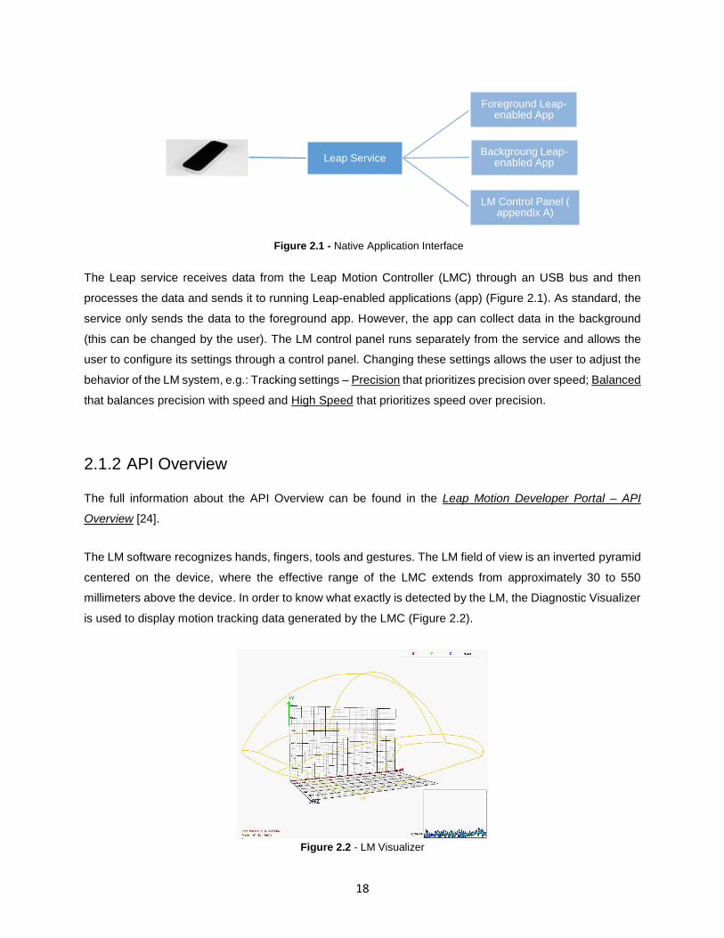
The Leap service receives data from the Leap Motion Controller (LMC) through an USB bus and then
processes the data and sends it to running Leap-enabled applications (app) (Figure 2.1). As standard, the
service only sends the data to the foreground app. However, the app can collect data in the background
(this can be changed by the user). The LM control panel runs separately from the service and allows the
user to configure its settings through a control panel. Changing these settings allows the user to adjust the
behavior of the LM system, e.g.: Tracking settings – Precision that prioritizes precision over speed; Balanced
that balances precision with speed and High Speed that prioritizes speed over precision.
2.1.2 API Overview
The full information about the API Overview can be found in the Leap Motion Developer Portal – API
Overview [24].
The LM software recognizes hands, fingers, tools and gestures. The LM field of view is an inverted pyramid
centered on the device, where the effective range of the LMC extends from approximately 30 to 550
millimeters above the device. In order to know what exactly is detected by the LM, the Diagnostic Visualizer
is used to display motion tracking data generated by the LMC (Figure 2.2).
Figure 2.2 - LM Visualizer
Leap Service
Foreground Leap-enabled App
Backgroung Leap-enabled App
LM Control Panel ( appendix A)
Figure 2.1 - Native Application Interface

19
This system uses the right-handed Cartesian coordinate system (Figure 2.3). The origin is centered at the
top of the device. The y-axis is vertical, with positive values increasing upwards and the z-axis has positive
values increasing toward the user. The unit used by the LM API to measure the distance is millimeters.
Figure 2.3 - The LM coordinate system (adapted from [24])
The LM is able to track hands, fingers and tools in its field of view and provides what it detects in a frame of
data. Each frame contains information of the tracked data describing the overall motion detected. When a
hand is detected, all the information about its motion is provided to the user. These motions are calculated
between two frames and can be used to define different interactions depending on what is intended. The
motions detected can be: Scale (e.g. one hand moves away to the other); Rotation (e.g. change of the
orientation of the hand); Translation (e.g. change of position of the palm of the hand). It’s also possible to
provide the list of the fingers and/or tools associated with the hand detected. For the fingers and tools, the
LM classifies finger or tool according to its shape, since normally a tool is longer, thinner and straighter than
a finger (Figure 2.4). For both cases, characteristics like the position or the direction vectors are provided
to the user.
Figure 2.4 - In red Fingers (left) and Tool detected (right) [24]
Lastly, another important feature present in this software is the ability to distinguish certain movements as
gestures. The gestures are detected for each finger or tool individually. Some of the gestures recognized
are: Circle – A finger or tool tracing a circle; Swipe – A linear movement of a finger or tool; Key tap – A
tapping movement by a finger or tool as if clicking in a key; and Screen tap – A tapping movement by the
finger or tool as if was touching the computer screen (Figure 2.5).

20
Figure 2.5 - LM recognized gestures [24]
2.1.3 An overview on the SDK and frame data
The full information about the Overview of the SDK and frame data can be found in the book Leap Motion
Development Essentials [25].
Along with the device software installation, the creators of the Leap Motion® also provide the SDK required
to the development of applications. This development kit is written in various languages (C + +, C # or Java)
and contains all the libraries, codes and headers necessary for the development of any project. To help the
user to develop his project, an extensive documentation is provided where it’s possible to find examples of
codes that can be used to create a new application, a more detailed description of each class (e.g.:
Leap::Vector, which represents a three-component mathematical vector or point such as a direction or
position in three-dimensional space) and the description of existing functions which, for example, can be
used for the calculation of the angle between two fingers (Leap::Vector::angleTo).
In the Leap SDK the following folders can be found:
docs — LM documentation with sample application tutorials;
samples —applications in some languages like C++, Objective-C and Java;
include — LM API header and source files to include in C++ and Objective-C applications;
lib — compile-time and runtime libraries for the supported languages;
util — utility classes;
examples — examples of applications.
The most important files present in this folders are the Leap.h, which contains the Leap C++ API class and
struct definitions, the LeapMath.h, which contains the Leap C++ API Vector and Matrix class and struct
21
definitions, the Leap.lib, which is a compile-time library, the Leap.dll, which is a runtime library, the Leapd.lib,
which is the compile-time debug library and finally the Leapd.dll, which is the runtime debug library.
The communication with the LM software is done through key classes that are already defined in the file
Leap.h. The class Leap::Controller provides the main interface between the LM and the application. This
class can track processed frames, give the connection state of the device and invoke callbacks from a
listener. For instance, the class Leap::Listener is used to interact with the software and implementing the
right callback function is possible to handle the events transmitted by the software. The callback used for
this work was onFrame due to the fact that this is the only callback that can dispatch data from what the
Leap Motion® Controller (LMC) is detecting. Basically, this function gets the latest frame of motion tracking
data detected and prints the information. The other existing callbacks only transmit information like if the
controller is connected or disconnected, or if the listener is removed, etc. [26]. An example of how to get a
frame of data is presented next [28]:
Leap::Controller controller = Leap::Controller(); Leap::Frame frame = controller.frame(); Leap::Hand hands = frame.hands(); Leap::Finger fingers = frame.fingers();
With the use of the function controller::frame is it possible get the newest frame object. This frame contains
information of the ID of the frame, the timestamp and lists of the hands, fingers, tools, and gestures tracked
in that frame. The class Leap::Hand provides information about the characteristics and movements of a
detected hand, as well as lists of the fingers and tools associated with the hand. The classes Leap::Finger
and Leap::Tool, contains, respectively, the physical characteristics of a detected finger and tool. The class
Leap::Pointable contains the physical characteristics of both fingers and tools, i.e. things which can be
pointed. Lastly, the class Leap::Gesturer, provides a recognized movement done by the user, i.e. for each
gesture detected, the LM adds a gesture object to the frame. (Figure 2.6)
The SDK provides also several math classes which can be used to describe matrixes, points, directions and
velocities. These classes are: Leap::Matrix and Leap::Vector, and can also provide several useful math
functions to work with vectors (e.g. cross(const Vector & other) – calculation of the cross product of a vector
with another vector) or matrixes (e.g. toMatrix3x3() which converts a Leap::Matrix object to another 3x3
matrix type).
Presently, only the fingers and the tools connected to certain hand are detected by the LM. However, it’s
possible to extract almost every information associated with each hand or finger. For instance, it’s possible
to detect the number of hands present in a frame, the position of each hand, its rotation, normal vectors,
gestures, velocity and direction. With the hand motion API it’s also possible to compare two frames and
determine the motion (translation, rotation or scale) of a specific hand. For a specific hand is also possible

22
to know if it has fingers or tools attached to the hand. This objects have many attributes describing their
movements, such as the tip position (position in mm from the LM origin), tip velocity (mm/s), direction
(pointing direction vector), length (mm), width (mm), etc.
Figure 2.6 - Hierarchy of the classes which constitute a frame
2.1.4 Limitations of the Leap Motion® v1
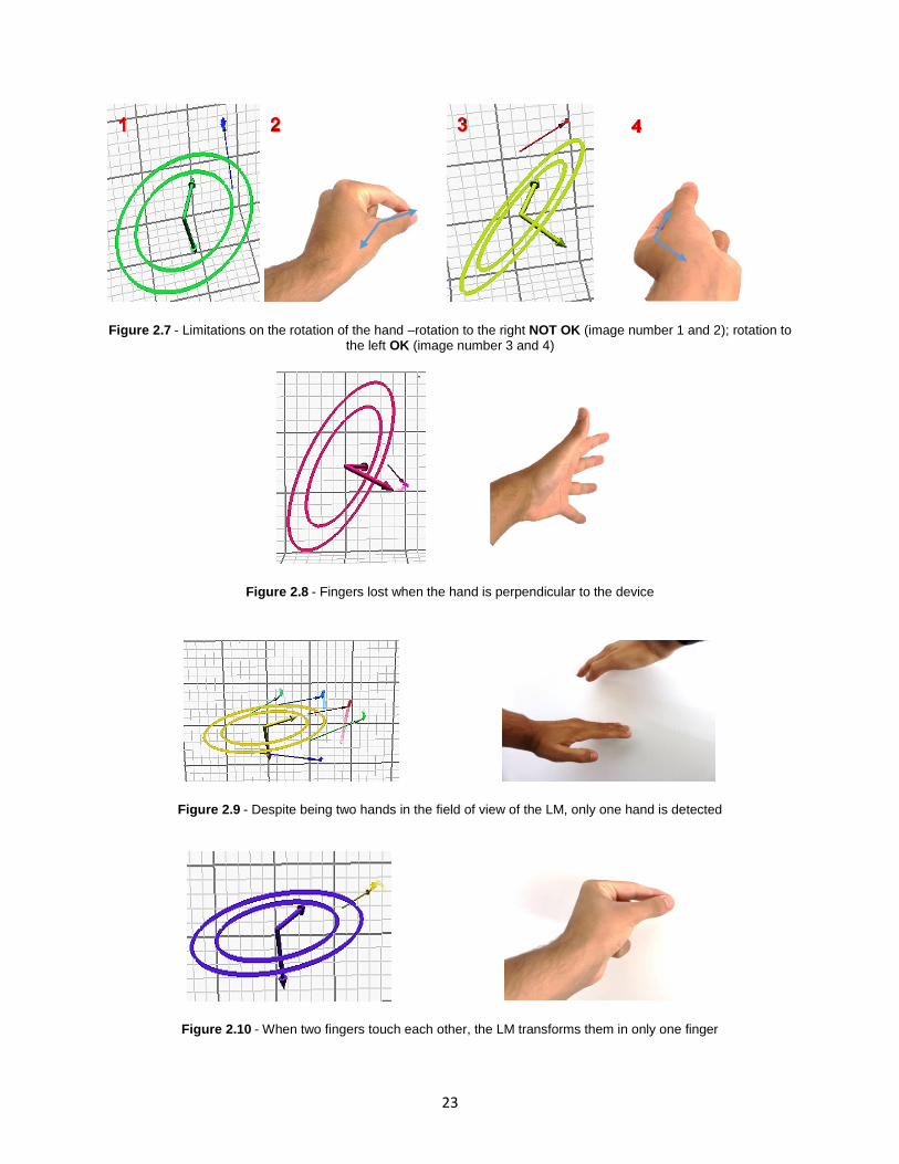
Due to the fact that it is the first version of this innovative technology, there are some limitations that should
be considered. Some of the most important limitations are:
Limitations on the rotation of the hand when it has less than 4 fingers (Figure 2.7);
LM loses track of the fingers if the hand is perpendicular to the device (Figure 2.8);
When the fingers are almost vertical, they start to “shake”;
Hands cannot be crossed since the LM loses track of the hands and fingers (Figure 2.9);
The LM doesn’t understand the interaction between fingers. If two fingers touch, the LM
automatically transforms these two fingers in only one finger (Figure 2.10);
Unstable tracking when close to the boundaries of the LM’s field of view (as Guna et al. [35]
referred - 1.3.2).
23
Figure 2.7 - Limitations on the rotation of the hand –rotation to the right NOT OK (image number 1 and 2); rotation to the left OK (image number 3 and 4)
Figure 2.8 - Fingers lost when the hand is perpendicular to the device
Figure 2.9 - Despite being two hands in the field of view of the LM, only one hand is detected
Figure 2.10 - When two fingers touch each other, the LM transforms them in only one finger
24
2.2 Leap Motion® v2
The full information about the newest version of the Leap Motion® can be found in the Leap Motion
Developer Portal – Introducing the Skeletal Tracking Model [29].
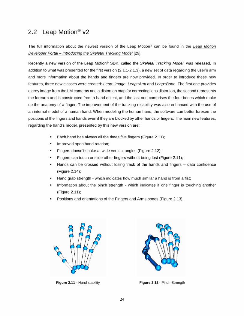
Recently a new version of the Leap Motion® SDK, called the Skeletal Tracking Model, was released. In
addition to what was presented for the first version (2.1.1-2.1.3), a new set of data regarding the user’s arm
and more information about the hands and fingers are now provided. In order to introduce these new
features, three new classes were created: Leap::Image, Leap::Arm and Leap::Bone. The first one provides
a grey image from the LM cameras and a distortion map for correcting lens distortion, the second represents
the forearm and is constructed from a hand object, and the last one comprises the four bones which make
up the anatomy of a finger. The improvement of the tracking reliability was also enhanced with the use of
an internal model of a human hand. When modeling the human hand, the software can better foresee the
positions of the fingers and hands even if they are blocked by other hands or fingers. The main new features,
regarding the hand’s model, presented by this new version are:
Each hand has always all the times five fingers (Figure 2.11);
Improved open hand rotation;
Fingers doesn’t shake at wide vertical angles (Figure 2.12);
Fingers can touch or slide other fingers without being lost (Figure 2.11);
Hands can be crossed without losing track of the hands and fingers – data confidence
(Figure 2.14);
Hand grab strength - which indicates how much similar a hand is from a fist;
Information about the pinch strength - which indicates if one finger is touching another
(Figure 2.11);
Positions and orientations of the Fingers and Arms bones (Figure 2.13).
Figure 2.12 - Pinch Strength Figure 2.11 - Hand stability

25
Figure 2.13 - Bone type Figure 2.14 - Data confidance
As it was said previously, the Image API allows the possibility to access to the raw data from the LM’s
infrared stereo cameras. This data can be used for computer vision, marker tracking, object recognition and
augmented reality. The data takes the form of a grayscale stereo image where, typically, the only objects
detected are those directly illuminated by the LMC LEDs. The API contains also a buffer with the sensor
brightness values and the camera calibration map, which can be used, for example, to correct lens
distortion.
Regarding the hierarchy of the frame, presented in the Figure 2.6 for the LM v1, a new scheme had to be
built in order to include the new features presented above. Below, an image showing the new scheme of
the LM v2 frame hierarchy is presented.
Figure 2.15 - Hierarchy of the classes which constitute a frame (v2) [40]
Besides these improvements, the software still has some limitations such as: fist poses may be unstable,
curling a finger may not work when making a fist, sometimes the hand can initialize flipped (upside-down),
the tracking quality is lower when making a fist or with less than 3 fingers extended, latency and CPU usage
are not yet optimized and finally, some limitations on the hand confidence.
26
2.3 Leap Motion® v1 vs Leap Motion® v2
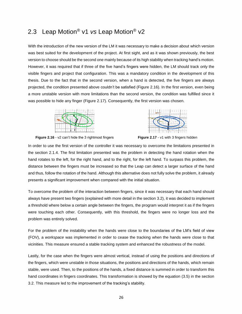
With the introduction of the new version of the LM it was necessary to make a decision about which version
was best suited for the development of the project. At first sight, and as it was shown previously, the best
version to choose should be the second one mainly because of its high stability when tracking hand’s motion.
However, it was required that if three of the five hand’s fingers were hidden, the LM should track only the
visible fingers and project that configuration. This was a mandatory condition in the development of this
thesis. Due to the fact that in the second version, when a hand is detected, the five fingers are always
projected, the condition presented above couldn’t be satisfied (Figure 2.16). In the first version, even being
a more unstable version with more limitations than the second version, the condition was fulfilled since it
was possible to hide any finger (Figure 2.17). Consequently, the first version was chosen.
Figure 2.16 - v2 can’t hide the 3 rightmost fingers Figure 2.17 - v1 with 3 fingers hidden
In order to use the first version of the controller it was necessary to overcome the limitations presented in
the section 2.1.4. The first limitation presented was the problem in detecting the hand rotation when the
hand rotates to the left, for the right hand, and to the right, for the left hand. To surpass this problem, the
distance between the fingers must be increased so that the Leap can detect a larger surface of the hand
and thus, follow the rotation of the hand. Although this alternative does not fully solve the problem, it already
presents a significant improvement when compared with the initial situation.
To overcome the problem of the interaction between fingers, since it was necessary that each hand should
always have present two fingers (explained with more detail in the section 3.2), it was decided to implement
a threshold where below a certain angle between the fingers, the program would interpret it as if the fingers
were touching each other. Consequently, with this threshold, the fingers were no longer loss and the
problem was entirely solved.
For the problem of the instability when the hands were close to the boundaries of the LM’s field of view
(FOV), a workspace was implemented in order to cease the tracking when the hands were close to that
vicinities. This measure ensured a stable tracking system and enhanced the robustness of the model.
Lastly, for the case when the fingers were almost vertical, instead of using the positions and directions of
the fingers, which were unstable in those situations, the positions and directions of the hands, which remain
stable, were used. Then, to the positions of the hands, a fixed distance is summed in order to transform this
hand coordinates in fingers coordinates. This transformation is showed by the equation (3.5) in the section
3.2. This measure led to the improvement of the tracking’s stability.

27
Chapter 3
3. The interface between Leap Motion® SDK
and MATLAB®
This chapter starts by describing the procedure done to perform the connection between MATLAB® and the
Leap Motion® controller using mex-functions. Next, it is presented the reason to emulate a human hand as
a surgical tool. And finally, it is presented the algorithm used to create the so called: hand’s model. This
model will be constructed with the data provided by the LMC and it will be used to control the EndoWrist®
instruments.
3.1 Matleap: The connection between Leap Motion® and
MATLAB®
The development of the hand’s model was done using the software MATLAB®, but, as it has been presented,
this language isn’t supported by the LMC. To perform the connection between this two programs, a
MATLAB® executable function (mex-function) was used. These functions compiles and links C, C++ or
FORTRAN files into binary mex-file that can be called from MATLAB®. The compiler used in this process
was the Microsoft Windows SDK 7.1.
To perform the creation of the mex-file, a set of files in a repository with the name Matleap [27] were used.
This repository can be found in the platform GitHub®, which is a web-based hosting service which enables
the sharing of any code with anyone. In this repository the most important files are: build.m, matleap.cpp,
matleap.h and test_matleap.m. The first function creates the mex-file that is needed to perform the
connection between MATLAB® and the LMC. To build that file, the mex command line is generated with the

28
following building options: –Ipathname; -Llibfolder; and –llibname. The first one is used to specify the path
to search for #include files, in this case the include folder from the Leap SDK where the Leap.h and
LeapMath.h, previously presented, are located. The last two options are used to specify the path to the
library file, in other words, the libname in the libfolder. In this case the libfolder is the directory
(...)/LeapSDK/lib/x64 and the libname is the Leap.lib file. The last command specifies the name of the C,
C++ or FORTRAN source file into a binary mex-file, in this case the source is the file matleap.cpp. The
command executed is the following: mex -I./LeapSDK/include -L./LeapSDK/lib/x64 -lLeap matleap.cpp.
Regarding the matleap.h and matleap.cpp, the first one is a header file which contains declarations that will
be used in the source file matleap.cpp. This source file contains the definitions of the declarations that are
present in the header.
In the header file is important to include the file that contains all the declarations necessary to perform the
connection with the LMC, to do that the command #include "Leap.h" is used. A struct called frame is also
created and contains the id of the detected frame, the timestamp, the pointables list (named pointables) and
the hands list (named hands). The key part of this header is the acquisition of a frame from the controller
which is made by using a structure (f) and contains all the information of the current frame. Lastly, the id,
timestamp, pointables attributes and hands attributes of that frame are saved in the structure current_frame
in order to be used in the matleap.cpp file.
Regarding the matleap.cpp, the existing version in the repository allows the acquisition of some attributes
detected by the LMC such as the information of the detected frame (id, timestamp and number of pointables
detected) and some other attributes concerning the pointables positions, directions and velocities. However,
these attributes aren’t enough to create a complete hand’s model since it requires the position of the hand,
the direction of the hand, axis of rotation, etc. To surpass this problem it was necessary to rewrite the code
in matleap.cpp in order to have access to more attributes. With the new matleap.cpp it’s now possible to
acquire the number of detected hands, the attributes of these hands, such as the approach direction, the
palm normal direction, the palm position and the stabilized palm position, and to obtain more attributes from
the pointables, such as the length and width of each pointable. All of these attributes will be needed to
create the hand’s model that will be used to control the EndoWrist® instruments. The creation of the hand’s
models will be explained in the section 3.2.
Regarding the code of this last file, the parameters nlhs and plhs represents the MATLAB® mex output
interface. The acquisition of the frame is done through the function created in the matleap.h file, get_frame,
and the creation of a MATLAB® frame structure with the names of the main classes present in the frame,
i.e. id, timestamp, hands and pointables.
Lastly, when the file test_matleap.m, which is an m-file created to test the connection between the LMC and
MATLAB®, is executed, a command is given to “let the hardware wake up” and then it gets a frame from the

29
LMC. To get a frame, the function matleap_frame.m is called and all that this function does is call the
matleap.cpp with the input value 1, which in the matleap.cpp code corresponds to the value of the variable
command. When the command is 1 the function get_frame (nlhs, plhs) in the .cpp file is executed and the
process of data collection is started. Then, the output of the function matleap_frame.m is stored in a variable
which now contains all the data acquired from the detected frame. Finally, the condition to have connection
between matleap.cpp and test_matleap.m, is that the designation of the vectors/arrays/doubles used in this
last one, have to have the same designation of its equivalents field names in the matleap.cpp and not its
equivalents in the LM notation. For example:
matleap.cpp
const char *pointable_field_names[] = { "position",
mxArray *pos = create_and_fill (f.pointables[i].tipPosition ()); LM notation = tipPosition
test_matleap.m
fprintf(' %f',f.pointables(i).position);
The test_matleap.m was also modified to present not only the pointables’ data but also the hands’ data in
the Command Window. The next section will show how this last m-file was useful for the creation of the
scripts used to perform the hand’s model.
3.2 MATLAB® hand’s model
To construct the hand’s model to control the EndoWrist® instruments two m-files were written. The main m-
file, leap2simulink.m, (appendix B) receives the following data from the LMC:
Hands (each hand) Pointables (each pointable)
Id Id
Palm Position Tip position
Palm Velocity Tip Velocity
Direction Direction
Palm Normal Length
Stabilized palm Position Width
and validates the configuration of the hands. This validation consists in the verification of the similarity
between a hand and the EndoWrist® instrument.
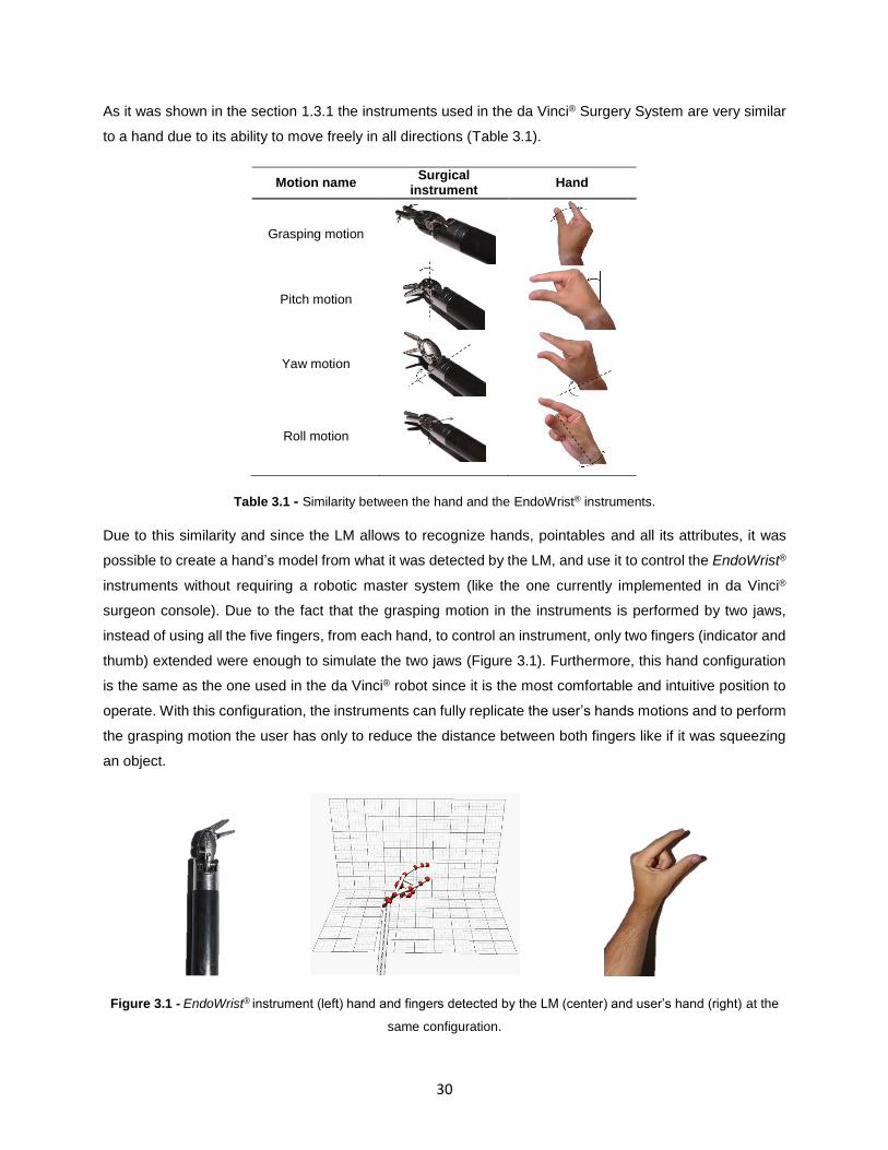
30
As it was shown in the section 1.3.1 the instruments used in the da Vinci® Surgery System are very similar
to a hand due to its ability to move freely in all directions (Table 3.1).
Table 3.1 - Similarity between the hand and the EndoWrist® instruments.
Due to this similarity and since the LM allows to recognize hands, pointables and all its attributes, it was
possible to create a hand’s model from what it was detected by the LM, and use it to control the EndoWrist®
instruments without requiring a robotic master system (like the one currently implemented in da Vinci®
surgeon console). Due to the fact that the grasping motion in the instruments is performed by two jaws,
instead of using all the five fingers, from each hand, to control an instrument, only two fingers (indicator and
thumb) extended were enough to simulate the two jaws (Figure 3.1). Furthermore, this hand configuration
is the same as the one used in the da Vinci® robot since it is the most comfortable and intuitive position to
operate. With this configuration, the instruments can fully replicate the user’s hands motions and to perform
the grasping motion the user has only to reduce the distance between both fingers like if it was squeezing
an object.
Figure 3.1 - EndoWrist® instrument (left) hand and fingers detected by the LM (center) and user’s hand (right) at the
same configuration.
Motion name Surgical
instrument Hand
Grasping motion
Pitch motion
Yaw motion
Roll motion
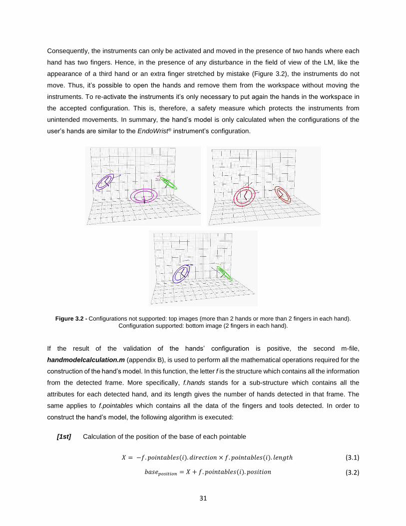
31
Consequently, the instruments can only be activated and moved in the presence of two hands where each
hand has two fingers. Hence, in the presence of any disturbance in the field of view of the LM, like the
appearance of a third hand or an extra finger stretched by mistake (Figure 3.2), the instruments do not
move. Thus, it’s possible to open the hands and remove them from the workspace without moving the
instruments. To re-activate the instruments it’s only necessary to put again the hands in the workspace in
the accepted configuration. This is, therefore, a safety measure which protects the instruments from
unintended movements. In summary, the hand’s model is only calculated when the configurations of the
user’s hands are similar to the EndoWrist® instrument’s configuration.
Figure 3.2 - Configurations not supported: top images (more than 2 hands or more than 2 fingers in each hand).
Configuration supported: bottom image (2 fingers in each hand).
If the result of the validation of the hands’ configuration is positive, the second m-file,
handmodelcalculation.m (appendix B), is used to perform all the mathematical operations required for the
construction of the hand’s model. In this function, the letter f is the structure which contains all the information
from the detected frame. More specifically, f.hands stands for a sub-structure which contains all the
attributes for each detected hand, and its length gives the number of hands detected in that frame. The
same applies to f.pointables which contains all the data of the fingers and tools detected. In order to
construct the hand’s model, the following algorithm is executed:
[1st] Calculation of the position of the base of each pointable
𝑋 = −𝑓. 𝑝𝑜𝑖𝑛𝑡𝑎𝑏𝑙𝑒𝑠(𝑖). 𝑑𝑖𝑟𝑒𝑐𝑡𝑖𝑜𝑛 × 𝑓. 𝑝𝑜𝑖𝑛𝑡𝑎𝑏𝑙𝑒𝑠(𝑖). 𝑙𝑒𝑛𝑔𝑡ℎ
𝑏𝑎𝑠𝑒𝑝𝑜𝑠𝑖𝑡𝑖𝑜𝑛 = 𝑋 + 𝑓. 𝑝𝑜𝑖𝑛𝑡𝑎𝑏𝑙𝑒𝑠(𝑖). 𝑝𝑜𝑠𝑖𝑡𝑖𝑜𝑛
(3.1)
(3.2)

32
With f.pointables.direction and f.pointables.position being vectors and f.pointables.length being
a scalar.
[2nd] Classification of the pointables as indicators and thumbs based on the x coordinate of the
baseposition of each pointable. The sorting rule is the following: the rightmost pointable is the right
indicator, the second rightmost is the right thumb, the third rightmost is the left indicator and the
last one is the left thumb (Figure 3.3).
Figure 3.3 - Classification of the pointables: 1-right indicator, 2-right thumb, 3-left thumb and 4-left indicator.
[3rd] Attribution to each finger its position.
[4th] Calculation of the angle between the two fingers of each hand. This measure will be used to
control the grip. The angle between two three-dimensional vectors is measured by the shortest
circle patch between them, which means that it must lie between 0 and pi radians. There are
two ways to calculate this angle. The first way uses the tangent (3.3) and the second one uses
the cosine (3.4). Due to a higher stability the formula that uses the tangent was chosen.
Being 𝑣1 and 𝑣2 three-dimensional vectors and 𝑣𝑎𝑣 the angle between them,
𝑣𝑎𝑣 = 𝑎𝑡𝑎𝑛2 (𝑛𝑜𝑟𝑚(𝑐𝑟𝑜𝑠𝑠(𝑣1, 𝑣2)), 𝑑𝑜𝑡(𝑣1, 𝑣2))
𝑣𝑎𝑣 = acos (𝑑𝑜𝑡(𝑣1, 𝑣2)
𝑛𝑜𝑟𝑚(𝑣1) × 𝑛𝑜𝑟𝑚(𝑣2)).
(3.3)
(3.4)

33
[5th] Classification of the hands as right hand or left hand. Figure 3.4 illustrates how this classification
is done.
Figure 3.4 - Hand’s Classification
[6th] Attribution to each hand its centralposition, approach direction, normal direction and calculation of the
centralfinger position using the equation (3.5) (Figure 3.5).
centralfinger position = centralposition + (𝑎𝑝𝑝𝑟𝑜𝑎𝑐ℎ 𝑑𝑖𝑟𝑒𝑐𝑡𝑖𝑜𝑛 × 𝑓𝑖𝑛𝑔𝑒𝑟𝑠𝑎𝑣𝑔 𝑙𝑒𝑛𝑔𝑡ℎ),
where 𝑓𝑖𝑛𝑔𝑒𝑟𝑠𝑎𝑣𝑔 𝑙𝑒𝑛𝑔𝑡ℎ stands for the average length of the two fingers in each hand.
Figure 3.5 - Hand’s attributes.
(3.5)
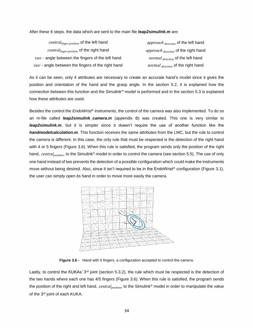
34
After these 6 steps, the data which are sent to the main file leap2simulink.m are:
centralfinger position of the left hand approach direction of the left hand
centralfinger position of the right hand approach direction of the right hand
𝑣𝑎𝑣 - angle between the fingers of the left hand normal direction of the left hand
𝑣𝑎𝑣 - angle between the fingers of the right hand normal direction of the right hand
As it can be seen, only 4 attributes are necessary to create an accurate hand’s model since it gives the
position and orientation of the hand and the grasp angle. In the section 5.2, it is explained how the
connection between this function and the Simulink® model is performed and in the section 5.3 is explained
how these attributes are used.
Besides the control the EndoWrist® instruments, the control of the camera was also implemented. To do so
an m-file called leap2simulink_camera.m (appendix B) was created. This one is very similar to
leap2simulink.m, but it is simpler since it doesn’t require the use of another function like the
handmodelcalculation.m. This function receives the same attributes from the LMC, but the rule to control
the camera is different. In this case, the only rule that must be respected is the detection of the right hand
with 4 or 5 fingers (Figure 3.6). When this rule is satisfied, the program sends only the position of the right
hand, centralposition, to the Simulink® model in order to control the camera (see section 5.5). The use of only
one hand instead of two prevents the detection of a possible configuration which could make the instruments
move without being desired. Also, since it isn’t required to be in the EndoWrist® configuration (Figure 3.1),
the user can simply open its hand in order to move more easily the camera.
Figure 3.6 - Hand with 5 fingers, a configuration accepted to control the camera.
Lastly, to control the KUKAs’ 3rd joint (section 5.3.2), the rule which must be respected is the detection of
the two hands where each one has 4/5 fingers (Figure 3.6). When this rule is satisfied, the program sends
the position of the right and left hand, centralposition, to the Simulink® model in order to manipulate the value
of the 3rd joint of each KUKA.
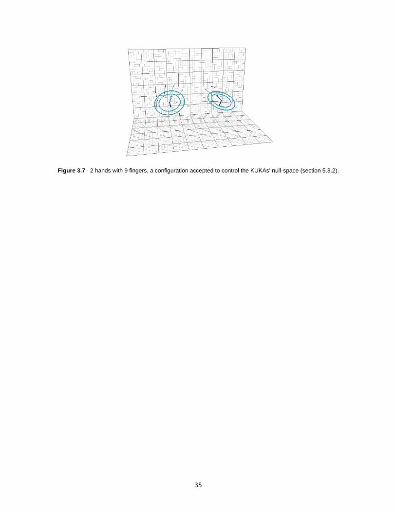
35
Figure 3.7 - 2 hands with 9 fingers, a configuration accepted to control the KUKAs' null-space (section 5.3.2).

36
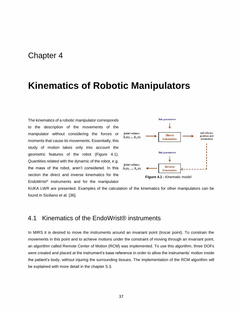
37
Chapter 4
4. Kinematics of Robotic Manipulators
The kinematics of a robotic manipulator corresponds
to the description of the movements of the
manipulator without considering the forces or
moments that cause its movements. Essentially, this
study of motion takes only into account the
geometric features of the robot (Figure 4.1).
Quantities related with the dynamic of the robot, e.g.
the mass of the robot, aren’t considered. In this
section the direct and inverse kinematics for the
EndoWrist® instruments and for the manipulator
KUKA LWR are presented. Examples of the calculation of the kinematics for other manipulators can be
found in Siciliano et al. [36].
4.1 Kinematics of the EndoWrist® instruments
In MIRS it is desired to move the instruments around an invariant point (trocar point). To constrain the
movements in this point and to achieve motions under the constraint of moving through an invariant point,
an algorithm called Remote Center of Motion (RCM) was implemented. To use this algorithm, three DOFs
were created and placed at the instrument’s base reference in order to allow the instruments’ motion inside
the patient’s body, without injuring the surrounding tissues. The implementation of the RCM algorithm will
be explained with more detail in the chapter 5.3.
Figure 4.1 - Kinematic model

38
4.1.1 Direct Kinematics
The direct kinematics allows to calculate the pose of the end-effector, namely the position and orientation,
of the robot in the workspace for a given set of joint variables. In other words, it maps the joint space in the
Cartesian space. The equation that describes the direct kinematics problem is:
𝑥𝑒 = 𝑘(𝑞).
Where 𝒙𝒆 describes the position 𝒑𝒆 and orientation ∅𝒆 of the end-effector.
𝑥𝑒 = [𝑝𝑒
∅𝑒]
The variable 𝒒 denotes the vector of joint variables.
𝑞 = [
𝑞1
⋮𝑞𝑛
]
Lastly, the vector function 𝒌(∙), nonlinear in general, allows the computation of the operational variables
from joint variables.
The first step to calculate the direct kinematics consists in defining a set of coordinate axes from the base
to the end-effector. To do that, the Denavit-Hartenber convention (DH) [36] is used. This convention defines
a coordinate frame to each join of the manipulator, and uses 4 parameters to describe the relation between
consecutive frames. These parameters are 𝑑𝑖, 𝑣𝑖, 𝑎𝑖 and 𝛼𝑖 and represent the translations and rotations
needed so that frames corresponding to two consecutive links coincide.
Figure 4.2 - DH kinematic parameters
(4.1)
(4.2)
(4.3)

39
The definitions of these parameters are:
𝒅𝒊 – Distance from the origin of the Frame i-1 to the intersection of the Zi-1 axis and the Xi axis along de
Zi-1 axis. In case of a prismatic joint this parameter is a variable.
𝒗𝒊 – Angle of rotation from the Xi-1 axis to the Xi axis about the Zi-1 axis. In case of revolute joint this
parameter is a variable.
𝒂𝒊 – Distance from the intersection of the Zi-1 axis and the Xi axis to the origin of the ith coordinate system
along the Xi axis.
𝜶𝒊 – Angle of rotation from the Zi-1 axis to the Zi axis about the Xi axis.
The position and orientation of the i-th frame coordinate can be expressed in the (i-1)th frame by the
following homogeneous transformation matrix 𝑻𝒊𝒊−𝟏(𝒒) [36].
𝑇𝑖𝑖−1(𝑞) = [
cos(𝑣𝑖) −sin(𝑣𝑖) cos(𝛼𝑖) sin(𝑣𝑖) sin(𝛼𝑖) 𝑎𝑖cos(𝑣𝑖)
sin(𝑣𝑖) cos(𝑣𝑖) cos(𝛼𝑖) − cos(𝑣𝑖) sin(𝛼𝑖) 𝑎𝑖sin(𝑣𝑖)0 sin(𝛼𝑖) cos(𝛼𝑖) 𝑑𝑖
0 0 0 1
] (𝑖 = 1,… , 𝑛).
The first step to obtain the function that describes the direct kinematic of the manipulator is the computation
homogeneous transformation 𝑇𝑛0(𝑞), that yields the position and orientation of the frame n with respect of
the frame 0. After that, and given 𝑇0𝑏 and 𝑇𝑒
𝑛, which represents respectively the position and orientation from
the base frame to the frame 0 and from the frame n to the end-effector frame, the calculation of the direct
kinematics function 𝑻𝒆𝒃(𝒒) is performed using (4.5).
𝑇𝑒𝑏(𝑞) = 𝑇0
𝑏𝑇𝑛0𝑇𝑒
𝑛
This function represents the position and orientation from the base frame to the end-effector frame, and its
result can be represented as follows.
𝑇𝑒𝑏(𝑞) = [ 𝑛𝑒
𝑏(𝑞) 𝑠𝑒𝑏(𝑞) 𝑎𝑒
𝑏(𝑞) 𝑝𝑒𝑏(𝑞)
0 0 0 1] = [
𝑅𝑒(𝑞) 𝑝𝑒(𝑞)
0𝑇 1]
Where 𝑛𝑒, 𝑠𝑒 , 𝑎𝑒 are the unit vectors of a frame attached to the origin of end-effector and represents the
rotation matrix 𝑅𝑒(𝑞). [36]
After introduced the method by which the direct kinematics is calculated, now it’s presented how it was
implemented on the EndoWrist® instrument. The Figure 4.3 illustrates how the coordinate axes were
distributed and the Table 4.1 presents the parameters of the DH matrix.
(4.4)
(4.5)
(4.6)
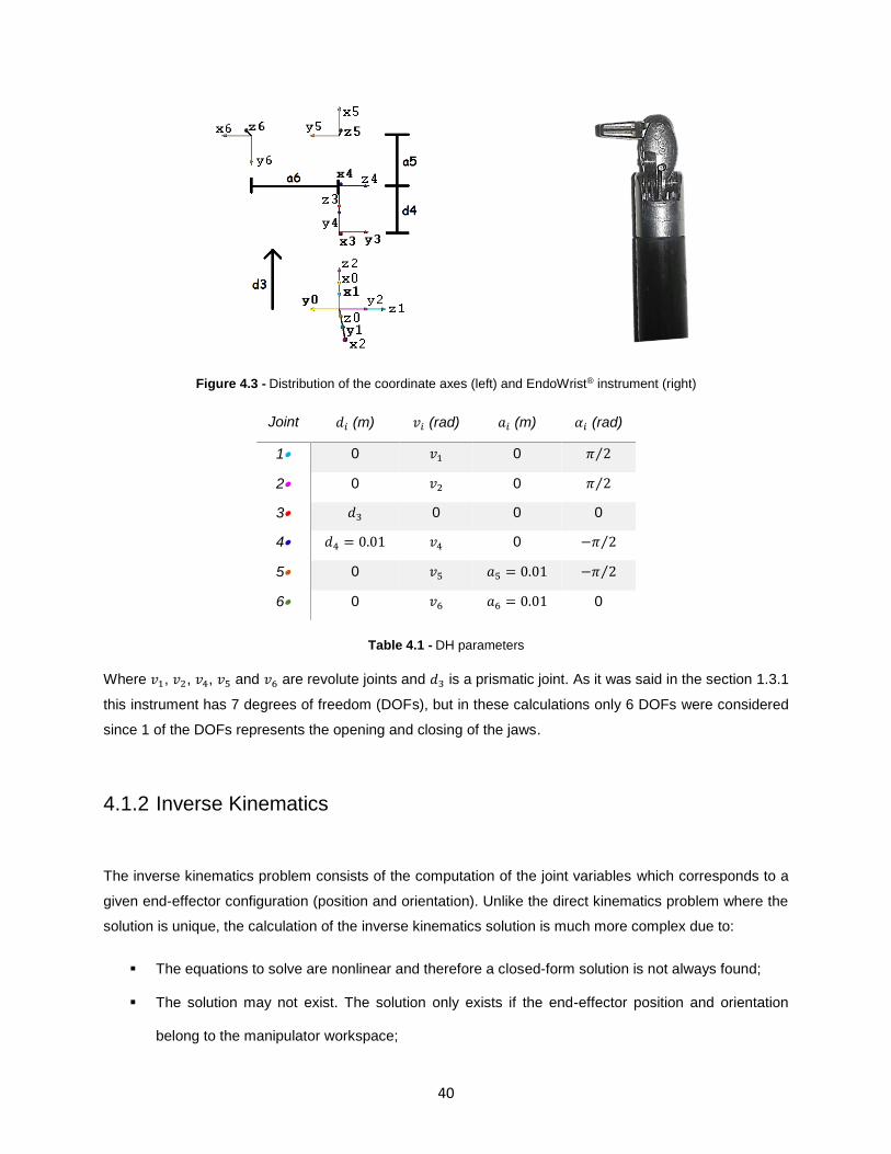
40
Figure 4.3 - Distribution of the coordinate axes (left) and EndoWrist® instrument (right)
Joint 𝑑𝑖 (m) 𝑣𝑖 (rad) 𝑎𝑖 (m) 𝛼𝑖 (rad)
1 0 𝑣1 0 𝜋 2⁄
2 0 𝑣2 0 𝜋 2⁄
3 𝑑3 0 0 0
4 𝑑4 = 0.01 𝑣4 0 −𝜋 2⁄
5 0 𝑣5 𝑎5 = 0.01 −𝜋 2⁄
6 0 𝑣6 𝑎6 = 0.01 0
Table 4.1 - DH parameters
Where 𝑣1, 𝑣2, 𝑣4, 𝑣5 and 𝑣6 are revolute joints and 𝑑3 is a prismatic joint. As it was said in the section 1.3.1
this instrument has 7 degrees of freedom (DOFs), but in these calculations only 6 DOFs were considered
since 1 of the DOFs represents the opening and closing of the jaws.
4.1.2 Inverse Kinematics
The inverse kinematics problem consists of the computation of the joint variables which corresponds to a
given end-effector configuration (position and orientation). Unlike the direct kinematics problem where the
solution is unique, the calculation of the inverse kinematics solution is much more complex due to:
The equations to solve are nonlinear and therefore a closed-form solution is not always found;
The solution may not exist. The solution only exists if the end-effector position and orientation
belong to the manipulator workspace;

41
Depending on the number of DOFs and number of non-null DH parameters, multiple solutions may
exist;
The solution may not be unique, e.g., a kinematically redundant manipulator has infinite solutions.
For the case of the EndoWrist® instrument, finding the analytical solution of the inverse kinematics is not
possible since it isn’t a structure of simple geometry. To solve this problem, an algorithm based on the
manipulator’s Jacobian is used. The name of this algorithm is Closed-Loop Inverse Kinematics (CLIK).
4.1.2.1 Closed-Loop Inverse Kinematics (CLIK)
The differential kinematics equation that characterize the relationship between the end-effector velocities (�̇�
- linear and 𝒘 - angular) and the joint velocities (�̇�) is given by:
�̇� = [�̇�𝑤
] = 𝐽(𝑞)�̇�,
where 𝑱 represents the manipulator geometric Jacobian. This Jacobian is a (6 × 𝑛) matrix, where 𝑛 is the
number of DOFs and can be partitioned into (3× 1) column vectors 𝐽𝑃𝑖 and 𝐽𝑂𝑖 as
𝐽 = [𝐽𝑃1 ⋯ 𝐽𝑃𝑛
⋮ ⋱ ⋮𝐽𝑂1 ⋯ 𝐽𝑂𝑛
],
where
[𝐽𝑃𝑖
𝐽𝑂𝑖] = {
[𝑧𝑖−1
0] 𝑓𝑜𝑟 𝑎 𝑝𝑟𝑖𝑠𝑚𝑎𝑡𝑖𝑐 𝑗𝑜𝑖𝑛𝑡
[𝑧𝑖−1 × (𝑝𝑒 − 𝑝𝑖−1)
𝑧𝑖−1] 𝑓𝑜𝑟 𝑎 𝑟𝑒𝑣𝑜𝑙𝑢𝑡𝑒 𝑗𝑜𝑖𝑛𝑡.
[36]
The vectors 𝑧𝑖−1, 𝑝𝑒 and 𝑝𝑖−1 are all functions of joint variables and have the following formulas [36]:
𝑧𝑖−1 = 𝑅10(𝑞1)… 𝑅𝑖−1
𝑖−2(𝑞𝑖−1)𝑧0,
𝑧0 = [0 0 1]𝑇 ,
𝑝𝑖−1 = 𝐴10(𝑞1)… 𝐴𝑖−1
𝑖−2(𝑞𝑖−1)𝑝0,
𝑝0 = [0 0 0 1]𝑇 and
𝑝𝑒 = 𝐴10(𝑞1)… 𝐴𝑛
𝑛−1(𝑞𝑛)𝑝0.
(4.7)
(4.8)
(4.9)
(4.10)
(4.11)
(4.12)
(4.13)
(4.14)
42
Considering that 𝑛 (number of DOF) equal to 𝑟 (number of operational space variables necessary to specify
a given task), 𝑛 = 𝑟 in the equation (4.7), the joint velocities can be obtained by simple inversion of the
Jacobian matrix 𝑱
�̇� = 𝐽−1(𝑞) �̇�.
However, (4.15) can only be computed when the Jacobian has full rank. When the manipulator is at a
singular configuration (4.15) cannot be used because (4.7) contains linearly dependent equations. Also, the
inversion of the Jacobian can represent a problem in a singularity or in the neighborhood of a singularity.
For example, the inversion of the Jacobian requires the computation of the determinant and in the
neighborhood of a singularity the determinant as a small value which cause large joint velocities. The
solution to overcome this problem is provided by the damped least-squares (DLS) inverse:
𝐽∗ = 𝐽𝑇(𝐽𝐽𝑇 + 𝑘2𝐼)−1,
where 𝑘 is a damping factor that allows the inversion of the Jacobian better conditioned from a numerical
viewpoint [36]. After obtaining the Jacobian to be used in the CLIK algorithm, it’s required to find a solution
to the equation (4.15). One solution is the time integration of this equation, however it’s necessary to escape
to the problem associated with the implementation of this solution in discrete time. To do that, an error that
it’s characterized by the difference between the desired position and orientation and the position and
orientation of the end-effector is used,
𝑒 = 𝑋𝑑 − 𝑋.
The (4.17) time derivate is
�̇� = 𝑋�̇� − �̇�
and when combined with (4.15) and (4.16) it’s obtained [36]
�̇� = 𝐽∗(𝑞) (�̇�𝑑 + 𝐾𝑒).
It’s also possible to verify that joining (4.19) and (4.7), the error 𝑒 goes to zero
�̇� + 𝐾𝑒 = 0.
where 𝐾 is a positive definite matrix which affects the convergence of the error to zero, in other words, the
increase of the eigenvalues of this matrix leads to a faster convergence to zero, however if these values are
too high the system will become unstable.
Like it was said before, the error 𝑒 is composed by to components – position and orientation. The end-
effector position error has the following formula:
𝑒𝑃 = 𝑝𝑑 − 𝑝(𝑞).
(4.15)
(4.16)
(4.17)
(4.18)
(4.19)
(4.20)
(4.21)

43
For the case of the end-effector orientation error, it’s necessary the combination between Euler angles and
unit quaternions. The reason of this combination is due to the existence of singularities in the representation
of the Euler angles [37]. To overcome this drawback the unit quaternion it’s used
𝑄 = {𝜂, 𝜖},
where 𝜂 is the scalar part and 𝜖 the vector part of the quaternion and have the following formulas [37]:
𝜂 = cos𝜗
2
𝜖 = sin𝜗
2𝑟 .
The rotation matrix, which now depends on 𝜂 and 𝜖, corresponding to a given quaternion has the following
formula [37]:
𝑅(𝜂, 𝜖) = (𝜂2 − 𝜖𝑇𝜖)𝐼 + 2𝜖𝜖𝑇 − 2𝜂𝑆(𝜖),
and the unit quaternion 𝑄 corresponding to a given rotation matrix is given by [37]:
𝜂 =1
2√𝑟11 + 𝑟22 + 𝑟33 + 1
𝜖 =
[ 1
2𝑠𝑖𝑔𝑛(𝑟32 − 𝑟23)√𝑟11 − 𝑟22 − 𝑟33 + 1
1
2𝑠𝑖𝑔𝑛(𝑟13 − 𝑟31)√𝑟11 − 𝑟22 − 𝑟33 + 1
1
2𝑠𝑖𝑔𝑛(𝑟21 − 𝑟12)√𝑟11 − 𝑟22 − 𝑟33 + 1]
.
Using 𝑅(𝑞) from the manipulator to calculate 𝑄, 𝑅𝑑 (desired orientation) to calculate also the unit quaternion
𝑄𝑑 and finally using 𝑆(∙),
𝑆(𝜖𝑑) = [
0 −𝜖3 𝜖2
𝜖3 0 −𝜖1
−𝜖2 𝜖1 0],
which a skew-symmetric operator, the end-effector orientation error based on quaternions has the following
formula [37]:
𝑒𝑂,𝑄𝑢𝑎𝑡 = 𝜂(𝑞)𝜖𝑑 − 𝜂𝑑𝜖(𝑞) − 𝑆(𝜖𝑑)𝜖(𝑞).
After all these steps, (4.19) now given by [37]:
�̇� = 𝐽∗(𝑞) [𝑝�̇� + 𝐾𝑃𝑒𝑃
𝑤𝑑 + 𝐾𝑂𝑒𝑂,𝑄𝑢𝑎𝑡],
(4.22)
(4.23)
(4.24)
(4.25)
(4.26)
(4.27)
(4.28)
(4.29)
(4.30)
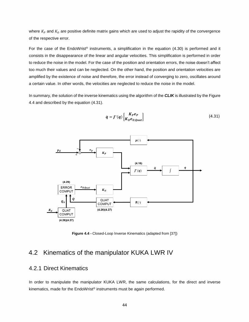
44
where 𝐾𝑃 and 𝐾𝑂 are positive definite matrix gains which are used to adjust the rapidity of the convergence
of the respective error.
For the case of the EndoWrist® instruments, a simplification in the equation (4.30) is performed and it
consists in the disappearance of the linear and angular velocities. This simplification is performed in order
to reduce the noise in the model. For the case of the position and orientation errors, the noise doesn’t affect
too much their values and can be neglected. On the other hand, the position and orientation velocities are
amplified by the existence of noise and therefore, the error instead of converging to zero, oscillates around
a certain value. In other words, the velocities are neglected to reduce the noise in the model.
In summary, the solution of the inverse kinematics using the algorithm of the CLIK is illustrated by the Figure
4.4 and described by the equation (4.31).
�̇� = 𝑱∗(𝒒) [𝑲𝑷𝒆𝑷
𝑲𝑶𝒆𝑶,𝑸𝒖𝒂𝒕]
Figure 4.4 - Closed-Loop Inverse Kinematics (adapted from [37])
4.2 Kinematics of the manipulator KUKA LWR IV
4.2.1 Direct Kinematics
In order to manipulate the manipulator KUKA LWR, the same calculations, for the direct and inverse
kinematics, made for the EndoWrist® instruments must be again performed.
(4.31)
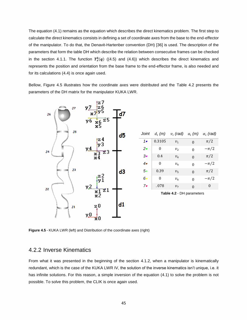
45
The equation (4.1) remains as the equation which describes the direct kinematics problem. The first step to
calculate the direct kinematics consists in defining a set of coordinate axes from the base to the end-effector
of the manipulator. To do that, the Denavit-Hartenber convention (DH) [36] is used. The description of the
parameters that form the table DH which describe the relation between consecutive frames can be checked
in the section 4.1.1. The function 𝑻𝒆𝒃(𝒒) ((4.5) and (4.6)) which describes the direct kinematics and
represents the position and orientation from the base frame to the end-effector frame, is also needed and
for its calculations (4.4) is once again used.
Bellow, Figure 4.5 illustrates how the coordinate axes were distributed and the Table 4.2 presents the
parameters of the DH matrix for the manipulator KUKA LWR.
Figure 4.5 - KUKA LWR (left) and Distribution of the coordinate axes (right)
4.2.2 Inverse Kinematics
From what it was presented in the beginning of the section 4.1.2, when a manipulator is kinematically
redundant, which is the case of the KUKA LWR IV, the solution of the inverse kinematics isn’t unique, i.e. it
has infinite solutions. For this reason, a simple inversion of the equation (4.1) to solve the problem is not
possible. To solve this problem, the CLIK is once again used.
Joint 𝑑𝑖 (m) 𝑣𝑖 (rad) 𝑎𝑖 (m) 𝛼𝑖 (rad)
1 0.3105 𝑣1 0 𝜋 2⁄
2 0 𝑣2 0 −𝜋 2⁄
3 0.4 𝑣4 0 𝜋 2⁄
4 0 𝑣4 0 −𝜋 2⁄
5 0.39 𝑣5 0 𝜋 2⁄
6 0 𝑣6 0 −𝜋 2⁄
7 . 078 𝑣7 0 0
Table 4.2 - DH parameters

46
4.2.2.1 Closed-Loop Inverse Kinematics (CLIK)
The differential equation that describes the relationship between the end-effector velocities (�̇� - linear and
𝒘 - angular) and the joint velocities (�̇�) is given by the equation (4.7), i.e.:
�̇� = [�̇�𝑤
] = 𝐽(𝑞)�̇�
In this equation, 𝑱 represents the manipulator geometric Jacobian and it has the formula presented in (4.8)
In order to formulate the geometric Jacobian the equation (4.9) is used, as well the equations (4.10) – (4.14).
Due to the redundancy of the manipulator, its Jacobian isn’t invertible because it isn’t quadratic, i.e. has
more columns than rows and thus infinite solutions exist. The solution to overcome this problem is the use
of the right pseudo-inverse of 𝑱, which has the following formula [36]:
𝐽† = 𝐽𝑇(𝐽𝐽𝑇)−1.
In the kinematically redundant manipulators, the Jacobian is affected by a null-space. The null-space of the
Jacobian is the subspace of joint velocities which don’t produce any movement at the end-effector at a given
posture. This can be described by the following formula [36]:
𝑁(𝐽(𝑞)) = {�̇� ∈ �̇�: 𝐽�̇� = 0}.
Reformulating (4.15), the equation that describes the solution for the inverse kinematics is given by [36]:
�̇� = 𝐽†(𝑞)�̇� + (𝐼 − 𝐽†(𝑞)𝐽(𝑞))𝑞0̇,
where the first term, 𝐽†�̇�, represents the particular solution for the inverse kinematics and the second
term, (𝐼 − 𝐽†𝐽)𝑞0̇, represents the homogeneous solution of the problem. In this second term, 𝑞0̇ represents
the set of joint velocities of the null-space and the matrix (𝐼 − 𝐽†𝐽) allows the projection of 𝑞0̇ in the null-
space of 𝑱. Like it was said above, if �̇� = 0, it is possible to generate internal motions described by the
second term of (4.35), which change the manipulator’s configuration without changing the end-effector
position and orientation [36]. The vector 𝑞0̇can be calculated using the following formula:
𝑞0̇ = 𝑘0 (𝜕𝑤(𝑞)
𝜕𝑞)
𝑇
,
where 𝑘0 > 0, 𝑤(𝑞) is an objective function of the joint variables and the gradient of 𝑤(𝑞), 𝜕𝑤(𝑞) 𝜕𝑞⁄ [36].
The choice of 𝑤(𝑞) depends on what is desired to make with the redundant DOFs, but typically the choices
are: the manipulability measure, where the redundancy is used to move the robot away from singularities,
the distance from mechanical joint limits, where the redundancy is used to keep the joints close to the center
of their ranges and lastly the distance from an obstacle, where the redundancy is used to avoid collision of
(4.32)
(4.33)
(4.34)
(4.35)
(4.36)
47
the manipulator with an obstacle [36]. For this manipulator, the distance from mechanical joint limits was
chosen in order to avoid the limits of the joints of the manipulator. For this case the objective function has
the following formula:
𝑤(𝑞) = −1
2𝑛∑(
𝑞𝑖 − �̅�𝑖
𝑞𝑖𝑀 − 𝑞𝑖𝑚
)2𝑛
𝑖=1
,
where 𝑞𝑖𝑀 and 𝑞𝑖𝑚 stands respectively for the maximum and minimum joint limits and �̅�𝑖 the middle value of
the joint range [36].
The solution of the first term of the equation (4.35), is achieved using an error that it’s characterized by the
difference between the desired position and orientation and the position and orientation of the end-effector
((4.17) and (4.18)). The solution of the inverse kinematics is then reformulated and can be written as follows:
�̇� = 𝐽†(𝑞)(�̇�𝑑 + 𝐾𝑒) + (𝐼 − 𝐽†(𝑞)𝐽(𝑞))𝑞0̇,
Like before, 𝐾 is a positive definite matrix which affects the convergence of the error to zero, in other words,
the increase of the eigenvalues of this matrix leads to a faster convergence to zero, however if these values
are too high the system will become unstable. It’s also possible to verify that 𝑒 goes to zero by the equation
(4.20) [36].
As in 4.1.2.1, the error has two components: the component of the position and the component of the
orientation. The component of the position is given by (4.21). To calculate the error of the orientation, the
unit quaternion is once again used. Thus, the equation which describes the orientation error is given by
(4.29). Combining (4.21) and (4.29) with (4.7), (4.37) is now given by:
�̇� = 𝐽†(𝑞) [𝑝�̇� + 𝐾𝑃𝑒𝑃
𝑤𝑑 + 𝐾𝑂𝑒𝑂,𝑄𝑢𝑎𝑡] + (𝐼 − 𝐽†(𝑞)𝐽(𝑞))𝑞0̇,
where 𝐾𝑃 and 𝐾𝑂 are positive definite matrix gains which are used to adjust the rapidity of the convergence
of the respective error.
Lastly, and as in the section 4.1.2.1, a simplification of the equation (4.39) is also performed and consists
in the disappearance of the linear and angular velocities. This simplification is performed in order to reduce
the noise in the model. For the case of the position and orientation errors, the noise doesn’t affect too much
their errors and can be neglected. On the other hand, the position and orientation velocities are amplified
by the existence of noise and therefore, the error instead of converging to zero, oscillates around a certain
value. In other words, the velocities are neglected to reduce the noise in the model.
In conclusion, the solution of the inverse kinematics, for the manipulator KUKA LWR IV, using the algorithm
of the CLIK is illustrated by the Figure 4.6 and described by the equation (4.40).
(4.37)
(4.38)
(4.39)

48
�̇� = 𝑱†(𝒒) [𝑲𝑷𝒆𝑷
𝑲𝑶𝒆𝑶,𝑸𝒖𝒂𝒕] + (𝑰 − 𝑱†(𝒒)𝑱(𝒒))𝒒�̇�
Figure 4.6 - Closed-Loop Inverse Kinematics (adapted from [37])
(4.40)
49
Chapter 5
5. Implementation of the model - KUKA
LWR IV + EndoWrist® instruments
In this chapter, a model comprised by two manipulators KUKA LWR IV and two EndoWrist® instruments
was developed. The model is controlled by the motions of the user’s hands which are read by the LMC. This
model works as an emulator of the real life model, i.e. it reproduce the kinematic behavior of the
manipulators KUKA and the surgical tools when controlled by the LM. The main goal of this implementation
was to detect and fix any existing imperfections and/or limitations in the kinematics of the manipulators and
evaluate the performance of the Leap Motion® in MIRS as a gestural master interface.
As such, this chapter presents the computational scheme adopted for the implementation of the model in
the Simulink® platform. This scheme is divided in four sections: the data acquisition; the implementation of
both CLIKs (presented in the previous chapter); the control of the footswitches; and the connection of the
Simulink® model (SM) with a virtual model of the KUKA LWR IV plus EndoWrist® instrument by means of a
Virtual Reality Modeling Language (VRML). It’s also proposed a design for the surgeon’s console to make
the model as close as possible to a surgical environment.
Lastly, the implemented model contains two identical KUKA + EndoWrist® assemblies to simulate a MIRS.
In order to avoid repeating the entire implementation for both assemblies, only the implementation of the
assembly which is controlled by the user’s right hand is presented. An image illustrating this model can be
found in the appendix C.
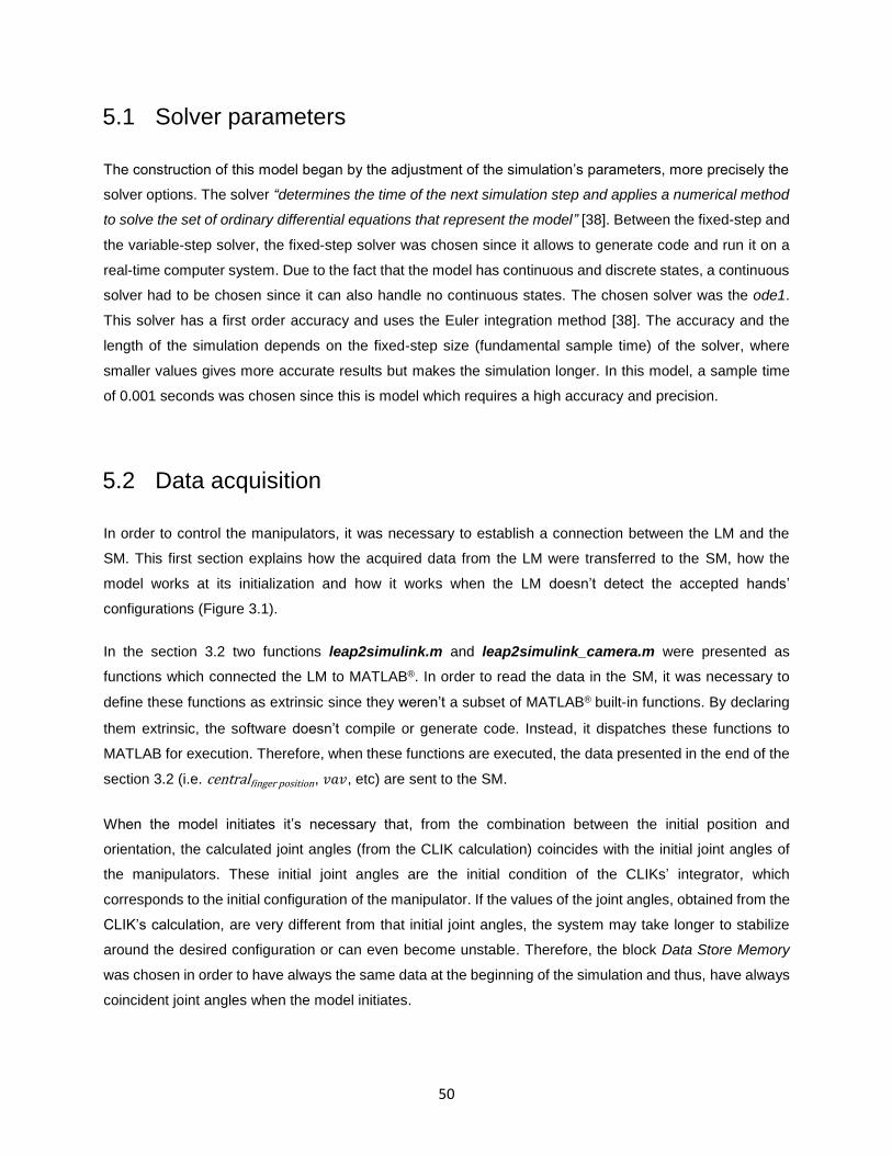
50
5.1 Solver parameters
The construction of this model began by the adjustment of the simulation’s parameters, more precisely the
solver options. The solver “determines the time of the next simulation step and applies a numerical method
to solve the set of ordinary differential equations that represent the model” [38]. Between the fixed-step and
the variable-step solver, the fixed-step solver was chosen since it allows to generate code and run it on a
real-time computer system. Due to the fact that the model has continuous and discrete states, a continuous
solver had to be chosen since it can also handle no continuous states. The chosen solver was the ode1.
This solver has a first order accuracy and uses the Euler integration method [38]. The accuracy and the
length of the simulation depends on the fixed-step size (fundamental sample time) of the solver, where
smaller values gives more accurate results but makes the simulation longer. In this model, a sample time
of 0.001 seconds was chosen since this is model which requires a high accuracy and precision.
5.2 Data acquisition
In order to control the manipulators, it was necessary to establish a connection between the LM and the
SM. This first section explains how the acquired data from the LM were transferred to the SM, how the
model works at its initialization and how it works when the LM doesn’t detect the accepted hands’
configurations (Figure 3.1).
In the section 3.2 two functions leap2simulink.m and leap2simulink_camera.m were presented as
functions which connected the LM to MATLAB®. In order to read the data in the SM, it was necessary to
define these functions as extrinsic since they weren’t a subset of MATLAB® built-in functions. By declaring
them extrinsic, the software doesn’t compile or generate code. Instead, it dispatches these functions to
MATLAB for execution. Therefore, when these functions are executed, the data presented in the end of the
section 3.2 (i.e. centralfinger position, 𝑣𝑎𝑣, etc) are sent to the SM.
When the model initiates it’s necessary that, from the combination between the initial position and
orientation, the calculated joint angles (from the CLIK calculation) coincides with the initial joint angles of
the manipulators. These initial joint angles are the initial condition of the CLIKs’ integrator, which
corresponds to the initial configuration of the manipulator. If the values of the joint angles, obtained from the
CLIK’s calculation, are very different from that initial joint angles, the system may take longer to stabilize
around the desired configuration or can even become unstable. Therefore, the block Data Store Memory
was chosen in order to have always the same data at the beginning of the simulation and thus, have always
coincident joint angles when the model initiates.
51
During the simulation, if the user removes its hands from the field of view of the LM or if the hands’
configurations don’t match the accepted configurations, it is important that the manipulators remain in the
last configuration until a new frame, which respects the rules, is detected. Therefore, if the hands’
configurations are correct, the provided data to the SM from leap2simulink.m/leap2simulink_camera.m
is calculated as in the section 3.2, if not, the data is still sent to the SM but this time it’s all made of zeros.
To keep the manipulators in the last configuration, the block verificação, which is a MATLAB Function, is
used. This block has two inputs and one output. The output is the already checked data which will be used
in the CLIKs and the inputs are the output from the functions leap2simulink.m (L2S) and the output of the
block Data Store Read (which copies all the data from the Data Store Memory to its output). In the
verificação block, it is verified if each element, from the acquisition function, is all made of zeros. If the result
of the verification is false, the output of verificação will have the value of the element from the acquisition
function. However, if the result is true, the output of verificação will have the value from element in the block
Data Store Read (DSR). For example, if the element centralfinger position (𝐿2𝑆) isn’t all made of zeros, the
element centralfinger position (𝑆𝑀) will have the value of the LS2’s element. If not, centralfinger position (𝑆𝑀) will
have the value of centralfinger position (𝐷𝑆𝑅) from the DSR. As the simulation goes by, the stored data is
updated by the block Data Store Write, which overwrites the existing data in Data Store Memory with the
output of the verificação block. This process is also performed for the data from the
leap2simulink_camera.m function.
Additionally, the model was implemented with a safety feature which guarantees that, after removing the
hands from the LM’s FOV, to reactivate the model, the hands must be placed close to the positions which
they were before being removed. This feature ensures the activation of the manipulators as close as
possible to its previous positions in order to prevent unintended movements.
5.3 CLIKs
The implementation of the kinematic of the manipulators can be performed by means of numeric methods
or symbolic methods. In order to obtain, prior to the start of the simulation, a mathematical model in terms
of time dependent parameters and variables, symbolic methods were used. This way, the model is only
generated once (before the execution of the simulation), which reflects in the reduction of the computational
weight during the simulation. Also, the use of auxiliary variables and mathematical tools, contribute to the
reduction of the computational weight.
To implement the combined kinematics of the manipulators, KUKA LWR and EndoWrist® instrument, two
different methods were studied. The first method consisted in the construction of a single CLIK which
included both manipulators. The second method consisted in the use of the two CLIKs, one for each
52
manipulator, connected in series, where the inputs of the second CLIK were calculated from the outputs of
the first CLIK. The construction of a single CLIK appeared to be the best option, but due to the fact that the
surgical instrument had to be manipulated around an invariant point, as it was presented in the section 4.1,
the CLIK would require a series of extra calculations [39] which would greatly increase the complexity of the
model and, therefore, increase its computational weight. In this model, the computational weight has an
extreme importance since its increase means also an increase of the delay on the manipulator’s motions,
which for this type of applications is unacceptable. With the use of two CLIKs in series, Figure 5.1, the
constraint at the trocar point could be easily surpassed with a simple implementation of the RCM algorithm
(section 5.3.3), without increasing the model’s computational weight.
Figure 5.1 - Implemented model with CLIKs in series
5.3.1 Coordinate Transformations: Pre-Instruments
The first block in the figure above, as the name indicates, performs the necessary operations to transform
the LM data in position and orientation for the CLIK, as well as for the control of the grasping motion (Right
graspº / Left graspº). Since there is a different configuration between the coordinate systems of the LM and
surgical tolls, a coordinate transformation was required to transform the position and direction vectors from
LM Cartesian space to EndoWrist® instrument Cartesian space. For the position, three operations were
performed: rotation of the axis of the LM in order to coincide with the axis of the instrument; conversion from
millimeters to meters; and configuration of the instrument’s workspace, i.e. translation of the LM’s origin to
the right in order to define the center of the right side of the LM’s FOV as the origin of the right hand (Figure
3.4). For the orientation, besides the rotation of the LM’s axis, since the LM only provides the approach and
normal direction, it was also necessary to calculate the slide direction. This vector was calculated by doing
the cross product between the other two directions. After having all the three vectors calculated and rotated,

53
the orientation matrix 𝑅𝑒(𝑞) was constructed using (4.6). The control of the grasp was almost straightforward
since the LM already provides the angle between the two fingers. However, and as it was explained in the
section 2.3, a threshold was necessary to indicate if the fingers were touching each other to avoid losing
track of the fingers. Therefore, it was established that if the angle between the fingers was smaller than 7º
the jaws would be fully closed and if the angle was greater than 13º the jaws would be fully open. Between
the 7º and 13º the jaws can vary its opening/closing gradually.
5.3.2 Instrument’s CLIK and KUKA’s CLIK
The instrument’s block has as inputs the position and orientation calculated in the previous block (presented
in the previous section). Regarding the outputs, the first output contains the resulting joint angles from the
first three instrument’s DOFs (𝑞1, 𝑞2 and 𝑞3), while the second output contains the remaining three joint
angles (𝑞4, 𝑞5 and 𝑞6).
The KUKA’s block has as inputs the position and orientation calculated in the RCM Algorithm block
(presented in the next section) and as output the results of the CLIK’s algorithm.
Figure 5.2 - Surgical Instrument’s DOFs
As it was presented in the section 4.1, the first three DOFs of the surgical instrument were created and
placed at the incision point to simulate the motion of the instrument around and along the trocar point. With
the attachment of the KUKA to the surgical instrument, instead of using these three virtual DOFs to simulate
the motions presented above, the virtual DOFs were used to calculate the position and orientation of the
KUKA’s end-effector needed to move the instrument around and along the trocar point, without injuring the
surrounding tissues (RCM Algorithm – section 5.3.3). Therefore, a model with a total of 11 DOFs (3 from
the surgical instrument (𝑞4, 𝑞5 and 𝑞6), 1 for the grasping motion and 7 from the KUKA) was used to control
the 7 DOFs (Figure 5.2) of the surgical instrument. These extra 4 DOFs makes the model kinematically
redundant which can be used to solve tasks whose movements are sophisticated like avoiding obstacles,
avoiding singular configurations, avoiding the limits of the manipulator’s joints, etc. In this case, the

54
redundancy was used to avoid the limits of the KUKA’s joints and the null-space of the KUKA’s Jacobian
was used to manipulate the value of its 3rd joint, without producing any movement at the end-effector. To
perform this manipulation, �̅�3, from the equation (4.37), was used as an input and its value is controlled by
the user’s hand (Figure 5.1).
5.3.3 RCM Algorithm
As it was said before, this block receives from the Instrument’s CLIK 𝑞1, 𝑞2 and 𝑞3, and calculates, through
the RCM algorithm, the position and orientation of the KUKA’s end-effector needed to move the instrument
around and along the trocar point. Therefore, the following equations were used:
Orientation
𝑅2𝑡 = 𝑅𝑜
𝑡𝑅20(𝑞
1, 𝑞
2),
where 𝑅𝑜𝑡 is a defined matrix which corresponds to the orientation of the KUKA’s end-effector at its
initial configuration. 𝑅20 is the orientation matrix from the frame 0 to the frame 2 of the surgical
instrument (Figure 4.3) and depends on its values 𝑞1 and 𝑞2. Lastly, the matrix 𝑅2𝑡 represents the
matrix 𝑅𝑡 rotated by means of the angles 𝑞1 and 𝑞2.
Position [41]
𝑏 = 𝐿 − 𝑞3,
𝑝𝐾𝑈𝐾𝐴 = 𝑝𝑡𝑟𝑜𝑐𝑎𝑟 + (𝑏 × �⃗� ),
where 𝐿 is the instrument length, 𝑏 the distance between the trocar and the KUKA’s end-effector,
𝑞3 is the distance between the trocar and the instrument end-effector, �⃗� the normal relative to the
instrument, 𝑝𝑡𝑟𝑜𝑐𝑎𝑟 the trocar position (constant) and lastly, 𝑝𝐾𝑈𝐾𝐴 the position of the KUKA’s end-
effector.
Figure 5.3 - KUKA (black), instrument (blue) and the position components to compute the RCM (adapted from [41])
(5.1)
(5.2)
(5.3)

55
The position 𝑝𝐾𝑈𝐾𝐴 and the orientation 𝑅2𝑡 are then used in the KUKA’s CLIK in order to obtain the
correspondent joint angles from that end-effector configuration. This algorithm guarantees the fulfilment of
the constraints at the trocar point, presented in 4.1, and provides the necessary DOFs to allow the
instrument to move around and along the trocar point, without injuring the surrounding tissues.
Besides the constraint presented above, another constraint at the trocar point was implemented. This new
constraint prevents the removal of the totality of the instrument from the patient’s interior while the surgery
is being performed. Therefore, it is only possible to remove the instrument from the interior of the patient
when the model is stopped. This constraint exists also in the Da Vinci® system, since the arms of the robot
can only be moved away from the incision point when the surgery ends.
5.4 Footswitches’ control
The footswitches’ control was a feature implemented to offer more freedom to the user. With this feature it
is possible to switch between controlling the manipulators and controlling the view point of the camera
without removing the hands from the LM’s workspace. Also, with the use of the footswitches it’s possible to
control the value of the 3rd KUKA’s joint in order to, for example, avoid obstacles.
To implement this feature, a Level-2 S-Function designed to accept keyboard input during the simulation,
combined with a switch system, was implemented in the SM. The detection of the key is possible by
retrieving the keyboard data, value associated to each key, from the window which appears when the
simulation starts. The value of the pressed key can then be used to perform multiple tasks. In this case it
was used to control a switch system. This system is composed by a Switch Case block and three Switch
Case Action Subsystem blocks. The first one receives the data to control the camera, the second receives
the data to control the manipulators and the third one is used to control the value of the 3rd KUKA’s joint
angle. The Switch Case vary between the case when the input has the value 32, which corresponds to the
value of the backspace, when is 13, which corresponds to the value of the enter, and the default case, which
can be any number except the 32 or 13. Therefore, if, for example, the backspace is pressed the view point
of the camera is controlled, the manipulators remains motionless and the KUKAs’ 3rd joint remains constant.
This was only possible due to the fact that the foot switches were emulated as keyboard keys (i.e. left pedal
– letter N, right pedal – backspace and middle pedal – ENTER).
5.5 Simulink® model – VRML
Analyzing the kinematic behavior of the manipulators can be a difficult task if the only results obtained are
from the CLIKs’ errors, which are calculated with the equations (4.21) and (4.29), and from the evolution of
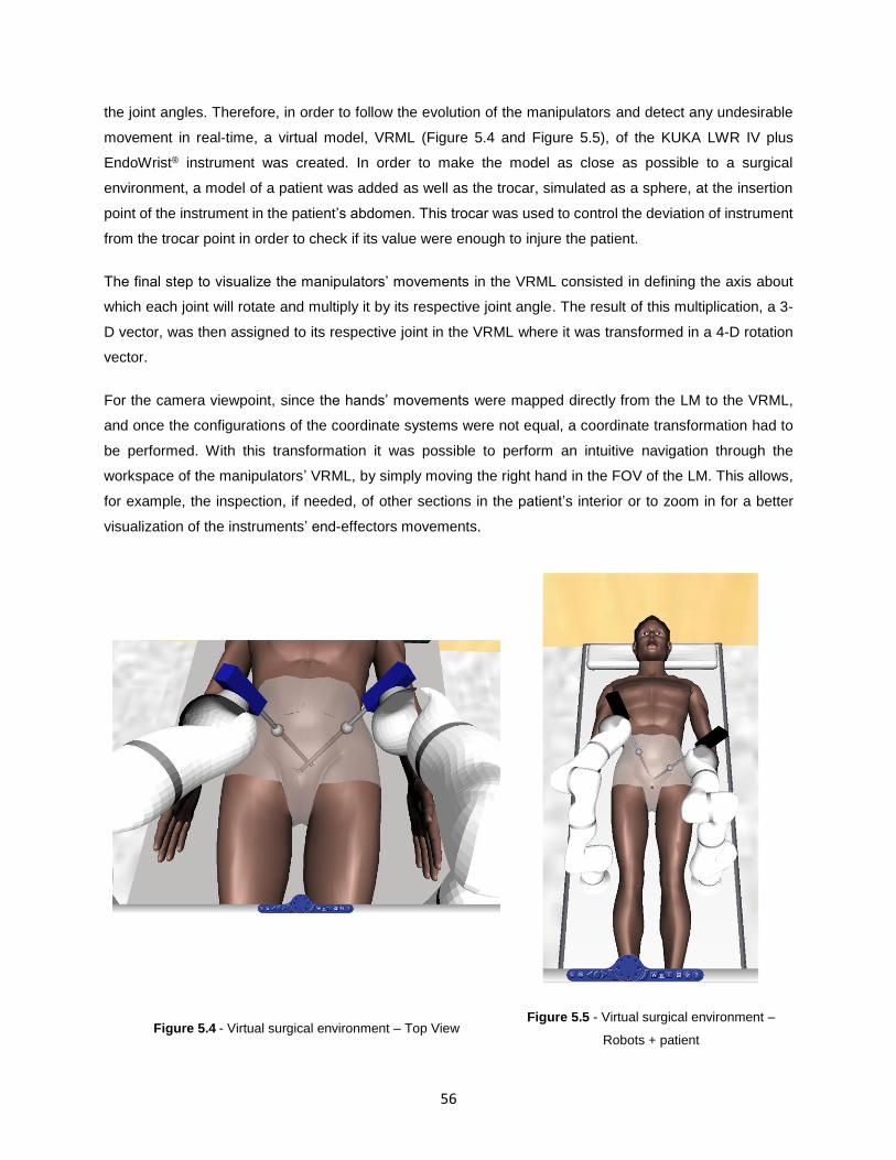
56
the joint angles. Therefore, in order to follow the evolution of the manipulators and detect any undesirable
movement in real-time, a virtual model, VRML (Figure 5.4 and Figure 5.5), of the KUKA LWR IV plus
EndoWrist® instrument was created. In order to make the model as close as possible to a surgical
environment, a model of a patient was added as well as the trocar, simulated as a sphere, at the insertion
point of the instrument in the patient’s abdomen. This trocar was used to control the deviation of instrument
from the trocar point in order to check if its value were enough to injure the patient.
The final step to visualize the manipulators’ movements in the VRML consisted in defining the axis about
which each joint will rotate and multiply it by its respective joint angle. The result of this multiplication, a 3-
D vector, was then assigned to its respective joint in the VRML where it was transformed in a 4-D rotation
vector.
For the camera viewpoint, since the hands’ movements were mapped directly from the LM to the VRML,
and once the configurations of the coordinate systems were not equal, a coordinate transformation had to
be performed. With this transformation it was possible to perform an intuitive navigation through the
workspace of the manipulators’ VRML, by simply moving the right hand in the FOV of the LM. This allows,
for example, the inspection, if needed, of other sections in the patient’s interior or to zoom in for a better
visualization of the instruments’ end-effectors movements.
Figure 5.4 - Virtual surgical environment – Top View Figure 5.5 - Virtual surgical environment –
Robots + patient
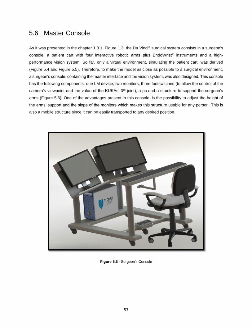
57
5.6 Master Console
As it was presented in the chapter 1.3.1, Figure 1.3, the Da Vinci® surgical system consists in a surgeon's
console, a patient cart with four interactive robotic arms plus EndoWrist® instruments and a high-
performance vision system. So far, only a virtual environment, simulating the patient cart, was derived
(Figure 5.4 and Figure 5.5). Therefore, to make the model as close as possible to a surgical environment,
a surgeon's console, containing the master interface and the vision system, was also designed. This console
has the following components: one LM device, two monitors, three footswitches (to allow the control of the
camera’s viewpoint and the value of the KUKAs’ 3rd joint), a pc and a structure to support the surgeon’s
arms (Figure 5.6). One of the advantages present in this console, is the possibility to adjust the height of
the arms’ support and the slope of the monitors which makes this structure usable for any person. This is
also a mobile structure since it can be easily transported to any desired position.
Figure 5.6 - Surgeon's Console

58

59
Chapter 6
6. Experimental Results
In this chapter it is presented the performance of the model presented in the previous chapter to perform
MIRS. First it is made the validation of the manipulators’ kinematics, introduced in the chapter 4, where it’s
studied the performance of the Closed-Loop Inverse Kinematics to solve the problem of the inverse
kinematics. After having the kinematics validated, it is verified the implementation of the RCM algorithm
which guarantees the fulfilment of the constraints at the trocar point, presented in 4.1, and allows the
instruments to move around and along the trocar point. Moreover, due to the fact that the CLIKs were
implemented in series, as showed in 5.3.2, a more detailed analysis is made in order to verify the existence
of delays which may degrade the performance of the model. Lastly, it is evaluated the performance of the
Leap Motion® to recognize the user’s movements. The results of this last topic allow the validation of the
manipulators’ movements not only around and along the trocar point, but also to validate the instrument’s
end-effector movements around a fixed point in space. It’s also important to refer that in the simulations
presented below, 0.1 seconds in simulation time is equivalent to 1 second in real life time.
6.1 Validation of the Kinematics
To validate de kinematics of the manipulators it’s necessary to evaluate the results of both direct and inverse
kinematics. The validation of the direct kinematics, for both manipulators, is straightforward since by
assigning values to the manipulators’ joints, it’s possible to check whether its position in space are correct
or incorrect. For this reason, the results of this verification aren’t showed. Regarding the inverse kinematics,
and since its calculation is not as simple as the direct kinematics, an evaluation of the CLIK’s performance
was made for both manipulators.
For the surgical instrument, to validate the inverse kinematics, it was applied to the manipulator a random
trajectory performed by the user’s hand, i.e. for each frame detected by the LM, the corresponding position

60
and orientation, from each hand, was sent to the CLIK in order to calculate the respective joint angles. The
reason for the random trajectory was due to the fact that it was intended to study how the model responded
to sudden variations. Having in mind what it was said in the chapter 4.1.2.1, both the position gain (𝐾𝑃) and
orientation gain (𝐾𝑂) are positive definite matrixes which affects the convergence of the error to zero, i.e.,
the increase of the eigenvalues of this matrix leads to a faster convergence to zero. However if these values
were too high the system would become unstable. After several iterations, it was concluded that the best
gains which guaranteed a fast movement of the instrument, with a position and orientation error of
magnitude 10−2, were: 𝐾𝑃 = 𝑑𝑖𝑎𝑔 {1000 1000 1000} and 𝐾𝑂 = 𝑑𝑖𝑎𝑔 {1000 1000 1000}. Regarding to 𝑘 ,from
the equation (4.16) to calculate 𝐽∗, two different values, 0.05 and 0.01, were tested in order to study its
influence in the evolution of the error.
Figure 6.1 - 𝑘 = 0.01: Reference (blue) vs CLIK result
(red)
Figure 6.2- k = 0.05: Reference (blue) vs CLIK result
(red)
As it can be seen by the two figures above, although the small difference between the values, 0.04, the
tracking error for 𝑘 = 0.05 is much larger than the tracking error when using 𝑘 = 0.01. As such, the value of
𝑘 = 0.01 was chosen since it provided an almost perfect tracking with a position error between
−5 × 10⁻³ and 5 × 10⁻³, and an orientation error between −2 × 10⁻² and 2 × 10⁻².
For the manipulator KUKA, a random trajectory performed by the user’s hand was also applied to validate
the CLICK algorithm. Once again, the reason for the random trajectory was due to the fact that it was
intended to study how the model responded to sudden variations. As it was said previously, it is intended to
use the redundancy to keep the joints close to the center of their ranges, i.e., avoid the joint limits. Table
6.1 shows the maximum and minimum joint limits angles, for each joint of the KUKA manipulator, used in
the equation (4.37), to solve the redundancy described in the chapter 4.2.2.1.
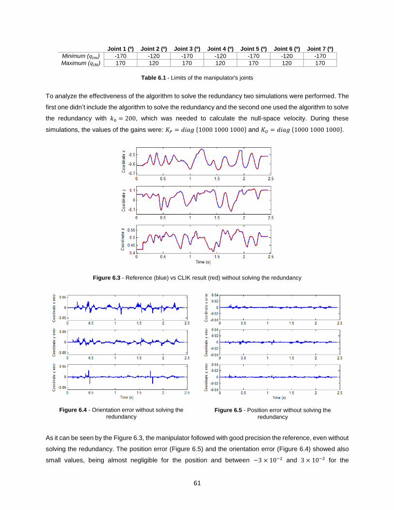
61
Joint 1 (º) Joint 2 (º) Joint 3 (º) Joint 4 (º) Joint 5 (º) Joint 6 (º) Joint 7 (º)
Minimum (𝑞𝑖𝑚) -170 -120 -170 -120 -170 -120 -170
Maximum (𝑞𝑖𝑀) 170 120 170 120 170 120 170
Table 6.1 - Limits of the manipulator's joints
To analyze the effectiveness of the algorithm to solve the redundancy two simulations were performed. The
first one didn’t include the algorithm to solve the redundancy and the second one used the algorithm to solve
the redundancy with 𝑘0 = 200, which was needed to calculate the null-space velocity. During these
simulations, the values of the gains were: 𝐾𝑃 = 𝑑𝑖𝑎𝑔 {1000 1000 1000} and 𝐾𝑂 = 𝑑𝑖𝑎𝑔 {1000 1000 1000}.
Figure 6.3 - Reference (blue) vs CLIK result (red) without solving the redundancy
Figure 6.4 - Orientation error without solving the
redundancy Figure 6.5 - Position error without solving the
redundancy
As it can be seen by the Figure 6.3, the manipulator followed with good precision the reference, even without
solving the redundancy. The position error (Figure 6.5) and the orientation error (Figure 6.4) showed also
small values, being almost negligible for the position and between −3 × 10⁻² and 3 × 10⁻² for the
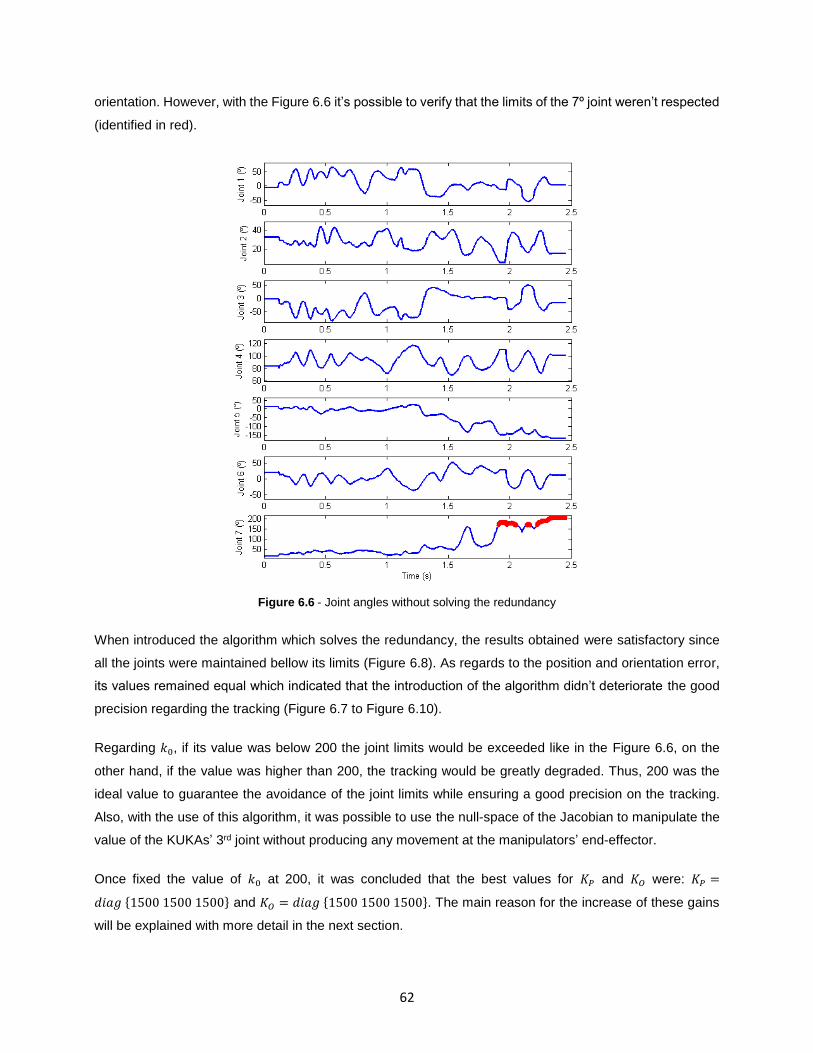
62
orientation. However, with the Figure 6.6 it’s possible to verify that the limits of the 7º joint weren’t respected
(identified in red).
Figure 6.6 - Joint angles without solving the redundancy
When introduced the algorithm which solves the redundancy, the results obtained were satisfactory since
all the joints were maintained bellow its limits (Figure 6.8). As regards to the position and orientation error,
its values remained equal which indicated that the introduction of the algorithm didn’t deteriorate the good
precision regarding the tracking (Figure 6.7 to Figure 6.10).
Regarding 𝑘0, if its value was below 200 the joint limits would be exceeded like in the Figure 6.6, on the
other hand, if the value was higher than 200, the tracking would be greatly degraded. Thus, 200 was the
ideal value to guarantee the avoidance of the joint limits while ensuring a good precision on the tracking.
Also, with the use of this algorithm, it was possible to use the null-space of the Jacobian to manipulate the
value of the KUKAs’ 3rd joint without producing any movement at the manipulators’ end-effector.
Once fixed the value of 𝑘0 at 200, it was concluded that the best values for 𝐾𝑃 and 𝐾𝑂 were: 𝐾𝑃 =
𝑑𝑖𝑎𝑔 {1500 1500 1500} and 𝐾𝑂 = 𝑑𝑖𝑎𝑔 {1500 1500 1500}. The main reason for the increase of these gains
will be explained with more detail in the next section.

63
Figure 6.7 - Reference (blue) vs CLIK result (red)
Figure 6.8 - Joint Angles
Figure 6.9 - Orientation error
Figure 6.10 - Position Error

64
6.2 Validation of the RCM Algorithm
In the beginning of this chapter it was introduced the problem of having the CLIKs in series, i.e., the
existence of delays when calculating the manipulators’ kinematics which could degrade the performance of
the model. In the end of the previous section, it was mentioned that 𝐾𝑃 and 𝐾𝑂 were increased from its initial
values 𝑑𝑖𝑎𝑔 {1000 1000 1000} to 𝑑𝑖𝑎𝑔 {1500 1500 1500}. The main reason for this increase was due to the
fact that the trocar constraint wasn’t being fulfilled as it should, i.e., instead of staying fixed at the trocar
point, the manipulator was moving at this point. This movement varied from 1 cm for slow movements of
the end-effector, to 2 cm for fast movements of the end-effector. Since the CLIKs are in series, the
calculation of the kinematics of the manipulators should be sequential, i.e., 1º - calculation of the joint angles
from the instrument’s CLIK; 2º calculation of the joint angles from the KUKA’s CLIK; and lastly 3º provide all
the joint angles to the VRML model. This way ensured that the joint angles would only be sent to the VRML
model when they were all calculated. However, Simulink® executes all the blocks at the same time which
means that, if there was a delay between the calculations of the kinematics of both manipulators, the VRML
model would receive joint angles that did not correspond all to the same integration step. This delay existed
since the KUKA’s CLIK needed more time than the instrument’s CLIK to converge the error to zero.
Therefore, this desynchronization made the convergence of the error to zero impossible while the
manipulators were in constant motion. The error equal to zero was only possible to achieve when the
manipulators were stopped. Hence, the existing delay did not allowed the joint angles to reach the required
values in time to maintain the manipulators fixed at the trocar point.
Figure 6.11 - Position error: displacement depending on the movements’ velocity

65
To overcome this delay, and as it was said at beginning of this section, the gains 𝐾𝑃 and 𝐾𝑂 were increased.
Since the values of the gains were higher than the gains used in the instrument’s CLIK
(𝑑𝑖𝑎𝑔 {1000 1000 1000} for both orientation and position), a faster convergence of the error to zero was
achieved and thus, the delay was decreased. With this solution, at a low or moderate velocity, the
displacement of the manipulator at the trocar point was now 0.1 cm, and at a high velocity the displacement
was now 1 cm (Figure 6.11). Higher values for 𝐾𝑃 and 𝐾𝑂 were also tried in order to reduce the delay but
instead of reducing the delay, the model became unstable making its use unfeasible.
Since a fast movement can produce a displacement of 1 cm of the instrument from the trocar point, it was
important to know what is considered as high velocity. From the experimental results, a velocity is
considered high when its value is around 2 𝑚/𝑠. As it has being presented in this thesis, the model here
presented is designed to use in MIRS, where the movements performed by the manipulators must be at a
slow or moderated velocity. Therefore, since in this type of application the manipulators aren’t move at
2 𝑚/𝑠, the displacement due to the movements at high velocity can be ignored.
The use of these new gains ensured also an improvement on the KUKA’s orientation error, since this error
went from varying between −3 × 10⁻² and 3 × 10⁻² to vary between −2 × 10⁻² and 2 × 10⁻² (Figure 6.12).
The KUKA’s position error had also improved, changing from varying between −10−2 and 10−2 to vary
between −5 × 10⁻³ and 5 × 10⁻³ (Figure 6.11).
Figure 6.12 - Orientation error: comparison between different movements' velocities
The remaining results, regarding the implemented model, can be viewed in the figures bellow (Figure 6.13
to Figure 6.20). The random trajectory was performed by the users’ hands. Again, the reason for the random
trajectory was due to the fact that it was intended to study how the model responded to sudden variations.
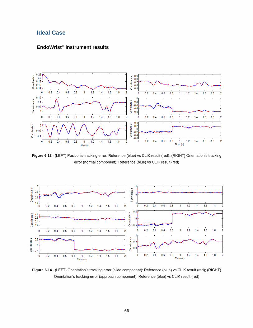
66
Ideal Case
EndoWrist® instrument results
Figure 6.13 - (LEFT) Position’s tracking error: Reference (blue) vs CLIK result (red); (RIGHT) Orientation’s tracking
error (normal component): Reference (blue) vs CLIK result (red)
Figure 6.14 - (LEFT) Orientation’s tracking error (slide component): Reference (blue) vs CLIK result (red); (RIGHT)
Orientation’s tracking error (approach component): Reference (blue) vs CLIK result (red)

67
Figure 6.15 - (LEFT) Orientation error; (RIGTH) Position error
Figure 6.16 - Joint angles

68
KUKA LWR IV results
Figure 6.17 - (LEFT) Position’s tracking error: Reference (blue) vs CLIK result (red); (RIGHT) Orientation’s tracking
error (normal component): Reference (blue) vs CLIK result (red)
Figure 6.18 - (LEFT) Orientation’s tracking error (slide component): Reference (blue) vs CLIK result (red); (RIGHT)
Orientation’s tracking error (approach component): Reference (blue) vs CLIK result (red)

69
Figure 6.19 - (LEFT) Orientation error; (RIGTH) Position error
Figure 6.20 - Joint angles

70
6.3 Validation of the Hands’ Movements
Validated the manipulators’ kinematics and the RCM algorithm, it is now necessary to validate also the
motion of the instrument around a fixed point in space. The analysis of these motions are of extreme
importance since its good precision and accuracy depends mainly on what is detected by the LMC. As it
was presented in the chapter 2, the selected version of the LMC has some limitations regarding the detection
of certain hand and fingers poses. In order to understand how these limitations influences the performance
of the model to perform surgery, several simulations were performed with the purpose to determine how
these limitations affected the tip’s motions. For these simulations, a fixed point in space was created to
study the tip movements around this point, therefore, in the following figures a red dot between the jaws
indicates that point.
Beginning with the 4th DOF of the surgical instrument (Figure 4.3), as it was described in the section 2.1.4,
the LM presents limitations in detecting the rotation of the hand when it has less than 4 fingers. A solution
to solve this problem was presented in the section 2.3, and consisted in increasing the distance between
the fingers so that the Leap can detect a larger hand surface and thus, follow more easily its rotation. Despite
the improvement with the implementation of this solution, when the movement is done with the right hand,
the rotation to the left isn’t yet fully achieved since the maximum reached angle was −33° when the jaws
were pointed forward (Figure 6.21 - 6a), and −10,5° when the jaws were pointed to the left (Figure 6.21 -
5b) (a full rotation corresponds to −90° or 90°). Moreover, when the jaws were pointed forward, it was clear
to verify that it was impossible to achieve the full rotation to the right (90°), since above the 80° the fingers
started to become superposed and the LM lost track of one of the fingers (Figure 6.21 - 3a). When the jaws
were pointed to the left, it was also impossible to reach the full rotation to the right (90°), since above the
60° the hand began to cover the fingers which stopped their tracking (Figure 6.21 - 3b).
For the instrument’s 5th DOF (Figure 4.3), Figure 6.22 shows the limitations when the user rotates his hand
upwards or downwards. When the jaws were pointed forward and the hand rotated was upwards (Figure
6.22 - 3a), the maximum reachable angle was 35°. The reason for the low value was due to the instability
of the fingers when they were almost vertical relatively to the device. Although it has been presented a
solution to this problem (fingers start to “shake”) in 2.3, the fingers end up disappearing from the LM’s FOV,
which stopped the hand’s tracking. When the hand rotates downwards (Figure 6.22 - 5a), the maximum
reachable angle was even smaller: −11°. The reason for this small value was due to the detection of the
curled fingers (particularly the knuckles) which stopped the hand’s tracking. When the jaws were pointed to
the left and the hand was rotated upwards (Figure 6.22 - 3b), the maximum reachable angle was 45° since
the fingers started to become superposed and the LM lost track of one of them. When the hand rotates
downwards (Figure 6.22 - 5b), the same limitation presented before, i.e., the detection of the knuckles of
the curled fingers, affected the detection of the correct hand configuration. Therefore, the maximum
reachable angle for this motion was only −7°.

71
Figure 6.21 - Limitations on the instrument's 4th DOF
Figure 6.22 - Limitations on the instrument's 5th DOF
1a 2a 3a 4a 5a 6a
1b 2b 3b 4b 5b
1a 2a 3a 4a 5a
1b 2b 3b 4b 5b
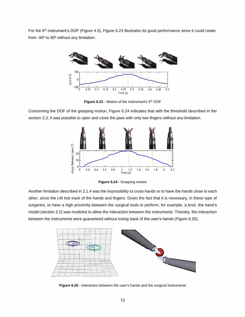
72
For the 6th instrument’s DOF (Figure 4.3), Figure 6.23 illustrates its good performance since it could rotate
from -90º to 90º without any limitation.
Figure 6.23 - Motion of the instrument's 6th DOF
Concerning the DOF of the grasping motion, Figure 6.24 indicates that with the threshold described in the
section 2.3, it was possible to open and close the jaws with only two fingers without any limitation.
Figure 6.24 - Grasping motion
Another limitation described in 2.1.4 was the impossibility to cross hands or to have the hands close to each
other, since the LM lost track of the hands and fingers. Given the fact that it is necessary, in these type of
surgeries, to have a high proximity between the surgical tools to perform, for example, a knot, the hand’s
model (section 3.2) was modeled to allow the interaction between the instruments. Thereby, the interaction
between the instruments were guaranteed without losing track of the user’s hands (Figure 6.25).
Figure 6.25 - Interaction between the user's hands and the surgical instruments
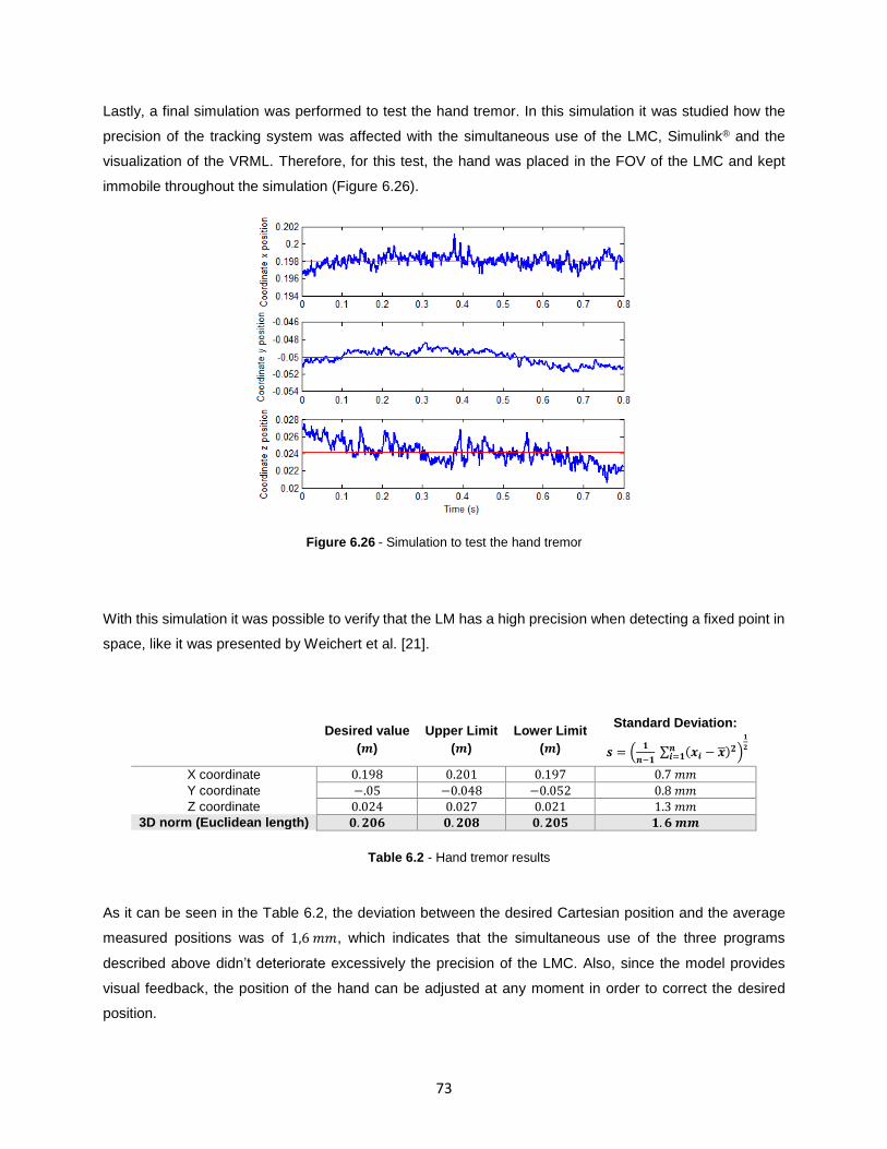
73
Lastly, a final simulation was performed to test the hand tremor. In this simulation it was studied how the
precision of the tracking system was affected with the simultaneous use of the LMC, Simulink® and the
visualization of the VRML. Therefore, for this test, the hand was placed in the FOV of the LMC and kept
immobile throughout the simulation (Figure 6.26).
Figure 6.26 - Simulation to test the hand tremor
With this simulation it was possible to verify that the LM has a high precision when detecting a fixed point in
space, like it was presented by Weichert et al. [21].
As it can be seen in the Table 6.2, the deviation between the desired Cartesian position and the average
measured positions was of 1,6 𝑚𝑚, which indicates that the simultaneous use of the three programs
described above didn’t deteriorate excessively the precision of the LMC. Also, since the model provides
visual feedback, the position of the hand can be adjusted at any moment in order to correct the desired
position.
Desired value
(𝒎)
Upper Limit
(𝒎)
Lower Limit
(𝒎)
Standard Deviation:
𝒔 = (𝟏
𝒏−𝟏 ∑ (𝒙𝒊 − �̅�)𝟐𝒏
𝒊=𝟏 )
𝟏
𝟐
X coordinate 0.198 0.201 0.197 0.7 𝑚𝑚
Y coordinate −.05 −0.048 −0.052 0.8 𝑚𝑚
Z coordinate 0.024 0.027 0.021 1.3 𝑚𝑚
3D norm (Euclidean length) 𝟎. 𝟐𝟎𝟔 𝟎. 𝟐𝟎𝟖 𝟎. 𝟐𝟎𝟓 𝟏. 𝟔 𝒎𝒎
Table 6.2 - Hand tremor results

74

75
Chapter 7
7. Conclusions and Further Work
The presented work focused in the implementation of a virtual surgical environment to perform MIRS
through a new gestural master interface. To create this new master, the Leap Motion® controller was used
since it allowed the user to interact with the software through hand gestures. Due to the similarity between
a hand and the EndoWrist® instrument, it was possible to create the hand’s model from what it was detected
by the LM, and use it to control the EndoWrist® instruments. Since it was desired to build the hand’s model
in MATLAB® and the LMC didn’t support this language, mex-functions were used to perform the connection
between these two software’s.
To control the manipulators in the Cartesian space, an algorithm to solve the inverse kinematics, named
CLIK, was implemented for each manipulator. An advantage with the use of this algorithm was the possibility
to use the redundancy of the manipulator KUKA to avoid its own joint limits. Also, with the use of this
algorithm, it was possible to use the null-space of the Jacobian to manipulate the value of the KUKAs’ 3rd
joint without producing any movement at the manipulators’ end-effector. The obtained results for both CLIKs
were satisfactory, since it was possible to move the manipulators in the Cartesian space with a small tracking
error (magnitude of 10−3).
The proposed implementation of the CLIKs in series was fully achieved with the application of the RCM
algorithm presented in this thesis. The results showed that this implementation didn’t degrade the model,
since the maximum displacement of the instrument at the trocar point for slow/moderate movements (<
2𝑚/𝑠) was of 1 mm. Therefore, it is possible to say that, for this model, the instruments are able achieve
motions under the constraint of moving through an invariant point, without injuring the surrounding tissues.
Regarding the limitations of the chosen LM version in detecting certain hand poses, it was possible to verify
that these limitations had a big impact when it was desired to move the instruments around a fixed point
space. The instrument’s 4th and 5th DOF were the most affected by these limitations. Both DOFs should
have had a range from −90° to 90°, but instead, they had a range of −11,5°/−33° to 60°/80° for the 4th DOF

76
and −11°/−7° to 35°/45° for the 5th DOF. As regards to the instrument’s 6th DOF and grasping motion, the
results showed that it was possible to achieve the full range of motion for these DOF since the LM’s
limitations didn’t influence directly their motions. Despite the good performance of these last DOFs, the
instrument’s performance will be always dependent on the poses of the 4th and 5th DOF which makes, for
example, the realization of a knot very difficult (if not even impossible) since the LM can’t neither fully rotate
a hand to the right or to the left, neither recognize superposed fingers, neither recognize the motion of an
inverted hand. Regardless these limitations, there were other limitations that were managed to be
surpassed, like for example: the possibility to have the hands close to each other which allowed the
interaction between the instruments; or the improvement of the model’s stability with the use of the hand
orientation instead the fingers orientation.
Finally, even with all the limitations presented above, it was still possible to simulate a surgical environment
with this new gestural master interface since the model provided features like: a robust workspace; different
hand configurations to control the instruments and the FOV of the camera; footswitch control to change
between controlling the instruments and controlling the camera; RCM algorithm to avoid injuring the patient
and to avoid the removal of the totality of the instrument while performing surgery; use of the KUKA’s
redundancy to avoid unwanted joint angles and the null-space of its Jacobian to manipulate the value of the
KUKA’s 3rd joint without producing any movement at the manipulators’ end-effector; and lastly, a simulation
without delays.
In summary, if the user restricts its hand’s movements to the poses that aren’t affected by the limitations
presented above, it is still possible to simulate a surgical environment since the created hand’s model
presents the appropriate robustness to be used as a gestural master interface.
7.1 Further Work
The presence of the limitations presented above inhibit the use of the full potential of the developed model.
This way, the next step, should focus in the improvement of the hands recognition system. The realization
of this improvement depends on how the LM is developed, i.e. if there is a possibility, in the future, to use
simultaneously two LM devices, the limitations regarding the full hand’s rotation and the superposed fingers
can be easily surpassed due to the increase of the LM’s FOV. If it isn’t possible to use two devices
simultaneously, a migration of the hand’s model from the version 1 to the version 2 of the LM should be
considered. Despite being more stable and robust than the first version and have the ability to collect the
images seen by the LM device, it should be kept in mind that, the hand’s model here created would have to
be completely redesigned since, in the 2nd version it isn’t possible to hide the fingers. The elimination of the
hand tremor is also possible with the use of filters, but it is suggested to have special attention in the
77
utilization of filters since it can degrade the performance of the model (e.g. delay the calculations which can
lead to the increase of the displacement at the trocar point). A final alternative proposed to overcome the
existent limitations, is the use of gestures to, for example, to perform a 180º rotation of the hand, and the
inverse gesture would make the hand back to its initial position. This way, it should be possible to overcome
the limitation of performing a full hand rotation. A more ambitious use of the gestures, would be the
assignment of certain actions to certain gestures and by doing that gesture, the correspondent action would
be triggered. For example, the execution of a single gesture would make the end-effector of the instrument
perform a knot.
Another suggestion to continue the work here developed, would be the implementation of a visual force
feedback. This feedback could be implemented through the use of instrumented trocars and force sensors
at instruments’ end-effector.
One last suggestion involves the use of the physical slaves, i.e. the real KUKA LWR IV and EndoWrist®
instruments that are in the Medical Robotics Laboratory of the IST Department of Mechanical Engineering.
This way, it would be possible to use the full surgical system in a physical environment.

78
79
References
[1] Treat., Michael R. "Computer-Integrated Surgery." A Surgeon's Perspective on the Difficulties of
Laparoscopic Surgery (MIT Press), 1995: 559-560.
[2] Long, K H, M P Bannon, S P Zietlow, E R Helgeson, W S Harmsen, C D Smith, D M Ilstrup, Y
Baerga-Varela, and M G Sarr. 2001. “A Prospective Randomized Comparison of Laparoscopic
Appendectomy with Open Appendectomy: Clinical and Economic Analyses.” Surgery 129 (4):
390–400. doi:10.1067/msy.2001.114216. http://www.ncbi.nlm.nih.gov/pubmed/11283528.
[3] Sauerland S, Lefering R, Neugebauer EAM. "Laparoscopic versus open surgery for suspected
appendicitis". Cochrane Database of Systematic Reviews 2004, Issue 4. Art. No.: CD001546.
DOI: 10.1002/14651858.CD001546.pub2.
[4] Pedersen, A. G., Petersen, O. B., Wara, P., Rønning, H., Qvist, N. and Laurberg, S. 2001,
"Randomized clinical trial of laparoscopic versus open appendicectomy". Br J Surg, 88: 200–
205. doi: 10.1046/j.1365-2168.2001.01652.x
[5] Intuitive Surgical, Inc. daVinci Surgery. 2014. http://www.davincisurgery.com/da-vinci-
gynecology/da-vinci-surgery/frequently-asked-questions.php (accessed 2014).
[6] Integrated Surgical Systems Inc. http://www.robodoc.com, April 2002.
[7] URS Universal Robot Systems. http://www.urs-group.com/orth/, April 2002
[8] Guthart, G.S., and J.K. Salisbury. 2000. “The Intuitive/sup TM/ Telesurgery System: Overview
and Application.” Proceedings 2000 ICRA. Millennium Conference. IEEE International
Conference on Robotics and Automation. Symposia Proceedings (Cat. No.00CH37065) 1. Ieee:
618–21. doi:10.1109/ROBOT.2000.844121.
http://ieeexplore.ieee.org/lpdocs/epic03/wrapper.htm?arnumber=844121
[9] Computer Motion Inc. http://www.computermotion.com, January 2002.
[10] Lanfranco, Anthony R, Andres E Castellanos, Jaydev P Desai, and William C Meyers. 2004.
“Robotic Surgery: A Current Perspective.” Annals of Surgery 239 (1): 14–21.
doi:10.1097/01.sla.0000103020.19595.7d.
http://www.pubmedcentral.nih.gov/articlerender.fcgi?artid=1356187&tool=pmcentrez&rendertype
=abstract.
[11] Taylor, Russell H, Arianna Menciassi, Gabor Fichtinger, and Paolo Dario. 2008. “Medical
Robotics and Computer-Integrated Surgery.” In Springer Handbook of Robotics, edited by Bruno
Siciliano and Khatib Oussama, 1199–1222. Springer Berlin Heidelberg. doi:10.1007/978-3-540-
30301-5_53. http://link.springer.com/referenceworkentry/10.1007%2F978-3-540-30301-5_53.

80
[12] Cadière, Guy-bernard, D Ph, Jacques Himpens, Olivier Germay, Rachel Izizaw, Michel
Degueldre, Jean Vandromme, Elie Capelluto, and Jean Bruyns. 2001. “Feasibility of Robotic
Laparoscopic Surgery : 146 Cases”, 1467–77. doi:10.1007/s00268-001-0132-2.
[13] Mitsuishi, Mamoru. 2007. “Minimally Invasive Surgery Robot and Master.” Complex Medical
Engineering, 2007. CME 2007. IEEE/ICME International Conference on Complex Medical
Engineering Medical, 8 – 13. doi:10.1109/ICCME.2007.4381682.
http://ieeexplore.ieee.org/xpls/abs_all.jsp?arnumber=4381682&tag=1.
[14] Madhani, Akhil Jiten. 1998. “Design of Teleoperated Surgical Instruments for Minimally Invasive
Surgery”. Massachussetts Institute of Technology.
[15] Palep, Jaydeep H. “Robotic Assisted Minimally Invasive Surgery.” J Minim Access Surg 5 (1): 1–
7. doi:10.4103/0972-9941.51313.
http://www.ncbi.nlm.nih.gov/pmc/articles/PMC2699074/?report=classic.
[16] Sun, Loi-wah, Frederick Van Meer, Yan Bailly, and Chung Kwong Yeung. 2007. “Design and D
Evelopment of a Da Vinci Surgical System S Imulator.” Proceedings of the 2007 IEEE -
International Conference on Mechatronics and Automation, 1050–55.
[17] Intuitive Surgery Inc. 2013. “The Da Vinci Surgery Experience.” doi:10.1007/s00464-011-1994-5.
http://www.davincisurgery.com/assets/docs/da-vinci-surgery-fact-sheet-en-
1005195.pdf?location=2&version=b.
[18] Intuitive Surgical,. 2014. http://www.intuitivesurgical.com/company/media/images/.
[19] Guthart, G.S., and J.K. Salisbury. 2000. “The IntuitiveTM Telesurgery System: Overview and
Application.” Proceedings 2000 ICRA. Millennium Conference. IEEE International Conference on
Robotics and Automation. Symposia Proceedings (Cat. No.00CH37065) 1. Ieee: 618–21.
doi:10.1109/ROBOT.2000.844121.
http://ieeexplore.ieee.org/lpdocs/epic03/wrapper.htm?arnumber=844121.
[20] Higuchi, Ty T, and Matthew T Gettman. 2011. “Robotic Instrumentation, Personnel and
Operating Room Setup.” In Atlas of Robotic Urologic Surgery, edited by Li-Ming Su, 15–30.
Totowa, NJ: Humana Press. doi:10.1007/978-1-60761-026-7.
http://link.springer.com/10.1007/978-1-60761-026-7.
[21] Weichert, Frank, Daniel Bachmann, Bartholomäus Rudak, and Denis Fisseler. 2013. “Analysis of
the Accuracy and Robustness of the Leap Motion Controller.” Sensors (Basel, Switzerland) 13
(5): 6380–93. doi:10.3390/s130506380.
http://www.pubmedcentral.nih.gov/articlerender.fcgi?artid=3690061&tool=pmcentrez&rendertype
=abstract.
[22] s.d. http://eftm.com.au/2013/08/control-your-pc-or-mac-with-gestures-using-the-leap-motion-
controller-video-11959.
[23] Motion, Leap. n.d.
https://developer.leapmotion.com/documentation/cpp/devguide/Leap_Architecture.html
(accessed 2014).

81
[24] Motion, Leap. n.d.
https://developer.leapmotion.com/documentation/csharp/devguide/Leap_Overview.html
(accessed 2014).
[25] Spiegelmock, Mischa. 2013. “Leap Motion SDK – A Quick Start.” In Leap Motion Development
Essentials, 11–13.
[26] Leap Motion Developer Portal. Getting Frame Data. s.d.
https://developer.leapmotion.com/documentation/cpp/devguide/Leap_Frames.html (accessed
2014).
[27] Inc, GitHub. jeffsp/matleap. n.d. https://github.com/jeffsp/matleap (accessed 2014).
[28] Carlos Vaz, Cristina Pestana, Paulo Roquete, César Resende. 2013. “Ileal Interposition
Reversal in Two Steps: Laparoscopic Normal Anatomy Reconstruction and Robotic Duodenal
Switch.” In Casos Clínicos Hospital Da Luz, edited by Espírito Santo Saúde, 1st ed., 133–38.
Lisboa: Jorge Fernandes, Lda.
[29] Motion, Leap. n.d.
https://developer.leapmotion.com/documentation/skeletal/cpp/devguide/Intro_Skeleton_API.html
(accessed 2014).
[30] Weede, O., H. Monnich, B. Muller, and H. Worn. 2011. “An Intelligent and Autonomous
Endoscopic Guidance System for Minimally Invasive Surgery.” 2011 IEEE International
Conference on Robotics and Automation, May. Ieee, 5762–68.
doi:10.1109/ICRA.2011.5980216.
http://ieeexplore.ieee.org/lpdocs/epic03/wrapper.htm?arnumber=5980216.
[31] Bischoff, Rainer, Johannes Kurth, Günter Schreiber, Ralf Koeppe, Alin Albu-schäffer, Der Beyer,
Oliver Eiberger, et al. 1993. “The KUKA-DLR Lightweight Robot Arm – a New Reference
Platform for Robotics Research and Manufacturing Summary / Abstract Stages of Research and
Product de- Velopment.”
[32] Haddadin, S, Ch Ott, A Stemmer, T Wimb, and G Hirzinger. “The DLR Lightweight Robot –
Design and Control Concepts for Robots in Human Environments.”
[33] German, Mechatronics. “DLR Lightweight Robots - Soft Robotics for Manipulation and
Interaction with Humans.”
[34] KUKA Lightweight Robot. n.d. http://f.metal-supply.com/2t4r60lvajkwlzxb.jpg (accessed 2014).
[35] Guna, Jože, Grega Jakus, Matevž Pogačnik, Sašo Tomažič, and Jaka Sodnik. 2014. “An
Analysis of the Precision and Reliability of the Leap Motion Sensor and Its Suitability for Static
and Dynamic Tracking”, 3702–20. doi:10.3390/s140203702.
[36] Siciliano, Bruno Lorenzo Sciavicco Luigi Luigi Villani, and Giuseppe Oriolo. 2009. Robotics:
Modelling, Planning and Control. Zhurnal Eksperimental’noi I Teoreticheskoi Fiziki. Springer.
doi:10.1007/978-1-84628-642-1.
http://scholar.google.com/scholar?hl=en&btnG=Search&q=intitle:No+Title#0.

82
[37] Chiaverini, Stefano, and Bruno Siciliano. 1999. “The Unit Quaternion: A Useful Tool for Inverse
Kinematics of Robot Manipulators.” Systems Analysis Modelling Simulation 35 (1). Gordon and
Breach Science Publishers, Inc. 45–60. http://portal.acm.org/citation.cfm?id=314865.
[38] MathWorks. Documentation Center: Simulink - Choosing a Solver Type. n.d.
http://www.mathworks.com/help/simulink/ug/choosing-a-solver.html (accessed 2014).
[39] Aghakhani, Nastaran, and Giuseppe Oriolo. 2013. “Task Control with Remote Center of Motion
Constraint for Minimally Invasive Robotic Surgery.” 2013 IEEE International Conference on
Robotics and Automation (ICRA), 5807–12.
[40] Davis, Alan. Leap Motion blog. s.d. http://blog.leapmotion.com/getting-started-leap-motion-sdk/
(accessed 2014).
[41] Osório, Diogo Filipe Roquette. 2013. “Robotic Assisted Arthroscopy for Hip Preserving Surgery
Diogo Filipe Roquette Osório Biomedical Engineering Examination Committee.”
https://fenix.tecnico.ulisboa.pt/downloadFile/395146026267/Robotic assisted arthroscopy for hip
preserving surgery.pdf

83
Appendix

84

85
A. Appendix A
Appendi x A: Leap Motion® Control Panel
Figure 0.1 A.1 - LM Control Panel

86
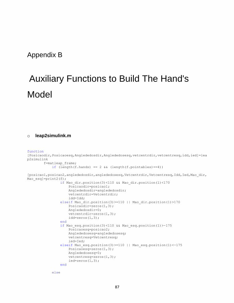
87
B. Appendix B
Appendi x A:Auxiliary Functions to Build The Hand's
Model
o leap2simulink.m
function
[Posicaodir,Posicaoesq,Anglededosdir,Anglededosesq,vetcentrdir,vetcentresq,idd,ied]=lea
p2simulink
f=matleap_frame;
if (length(f.hands) == 2 && (length(f.pointables)==4))
[posicao1,posicao2,anglededosdir,anglededosesq,Vetcentrdir,Vetcentresq,Idd,Ied,Mao_dir,
Mao_esq]=print2(f);
if Mao_dir.position(3)<110 && Mao_dir.position(1)<170
Posicaodir=posicao1;
Anglededosdir=anglededosdir;
vetcentrdir=Vetcentrdir;
idd=Idd;
elseif Mao_dir.position(3)>=110 || Mao_dir.position(1)>170
Posicaodir=zeros(1,3);
Anglededosdir=0;
vetcentrdir=zeros(1,3);
idd=zeros(1,3);
end
if Mao_esq.position(3)<110 && Mao_esq.position(1)>-175
Posicaoesq=posicao2;
Anglededosesq=anglededosesq;
vetcentresq=Vetcentresq;
ied=Ied;
elseif Mao_esq.position(3)>=110 || Mao_esq.position(1)<-175
Posicaoesq=zeros(1,3);
Anglededosesq=0;
vetcentresq=zeros(1,3);
ied=zeros(1,3);
end
else
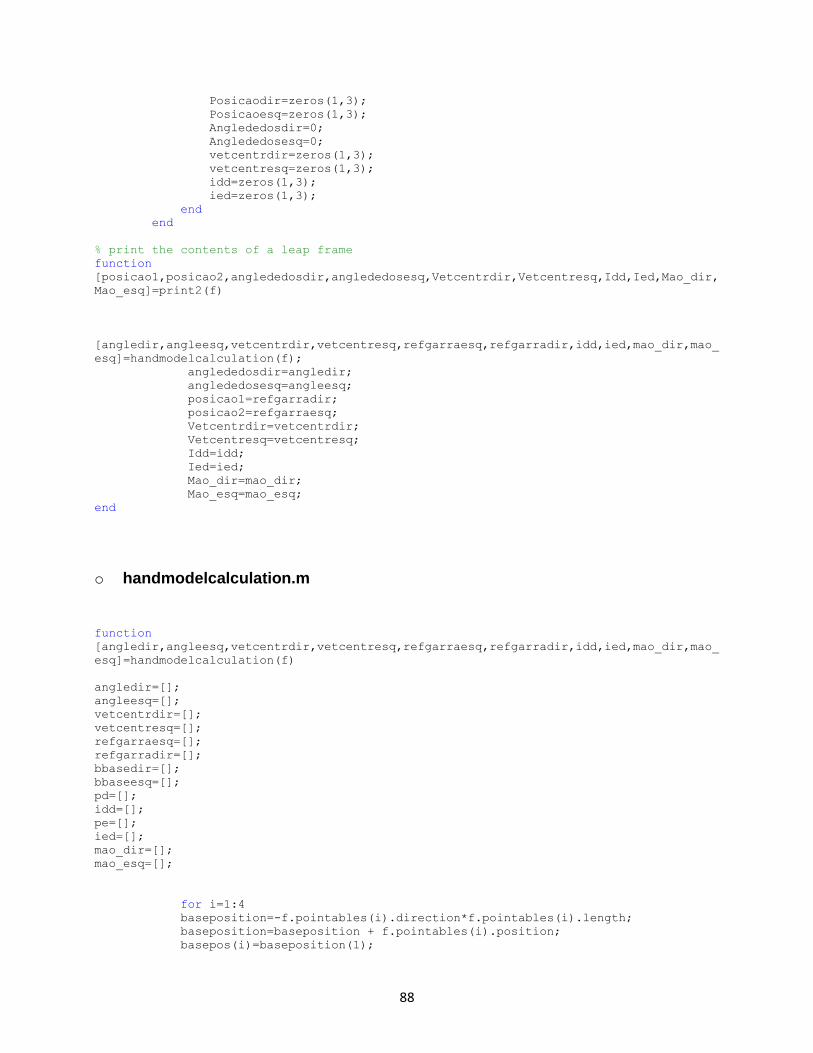
88
Posicaodir=zeros(1,3);
Posicaoesq=zeros(1,3);
Anglededosdir=0;
Anglededosesq=0;
vetcentrdir=zeros(1,3);
vetcentresq=zeros(1,3);
idd=zeros(1,3);
ied=zeros(1,3);
end
end
% print the contents of a leap frame
function
[posicao1,posicao2,anglededosdir,anglededosesq,Vetcentrdir,Vetcentresq,Idd,Ied,Mao_dir,
Mao_esq]=print2(f)
[angledir,angleesq,vetcentrdir,vetcentresq,refgarraesq,refgarradir,idd,ied,mao_dir,mao_
esq]=handmodelcalculation(f);
anglededosdir=angledir;
anglededosesq=angleesq;
posicao1=refgarradir;
posicao2=refgarraesq;
Vetcentrdir=vetcentrdir;
Vetcentresq=vetcentresq;
Idd=idd;
Ied=ied;
Mao_dir=mao_dir;
Mao_esq=mao_esq;
end
o handmodelcalculation.m
function
[angledir,angleesq,vetcentrdir,vetcentresq,refgarraesq,refgarradir,idd,ied,mao_dir,mao_
esq]=handmodelcalculation(f)
angledir=[];
angleesq=[];
vetcentrdir=[];
vetcentresq=[];
refgarraesq=[];
refgarradir=[];
bbasedir=[];
bbaseesq=[];
pd=[];
idd=[];
pe=[];
ied=[];
mao_dir=[];
mao_esq=[];
for i=1:4
baseposition=-f.pointables(i).direction*f.pointables(i).length;
baseposition=baseposition + f.pointables(i).position;
basepos(i)=baseposition(1);

89
end
z = [basepos(1) basepos(2) basepos(3) basepos(4)];
r = sort(z,'descend');
indicador_mao_direita = f.pointables(find(z==r(1)));
polegar_mao_direita = f.pointables(find(z==r(2)));
indicador_mao_esquerda = f.pointables(find(z==r(4)));
polegar_mao_esquerda = f.pointables(find(z==r(3)));
z = [f.hands(1).position(1) f.hands(2).position(1)];
r = sort(z,'descend');
mao_dir=f.hands(find(z==r(1)));
mao_esq=f.hands(find(z==r(2)));
id=indicador_mao_direita.position;
pd=polegar_mao_direita.position;
idd=mao_dir.yaw;
angledir=atan2(norm(cross(id,pd)), dot(id,pd));
angledir=rad2deg(angledir);
vetcentrdir=mao_dir.direction;
refgarradir=mao_dir.position;
ie=indicador_mao_esquerda.position;
pe=polegar_mao_esquerda.position;
ied=mao_esq.yaw;
angleesq=atan2(norm(cross(ie,pe)), dot(ie,pe));
angleesq=rad2deg(angleesq);
vetcentresq=mao_esq.direction;
refgarraesq=mao_esq.position;
end
o leap2simulink_camera.m
% leitura dos dados do leap
function [Posicao]=leap2simulink_camara
f=matleap_frame;
if (length(f.hands) == 1 &&
(length(f.pointables)>=4&&length(f.pointables)<=5))
Posicao=f.hands(1).position;
else
Posicao=zeros(1,3);
end
if (length(f.hands) == 2 &&
(length(f.pointables)>=8&&length(f.pointables)<=10))
z = [f.hands(1).position(1) f.hands(2).position(1)];
r = sort(z,'descend');
mao_dir=f.hands(find(z==r(1)));
mao_esq=f.hands(find(z==r(2)));
posicaodir=mao_dir.position(1);
posicaoesq=mao_esq.position(1);
else
posicaodir=1000;
posicaoesq=1000;
end
end

90
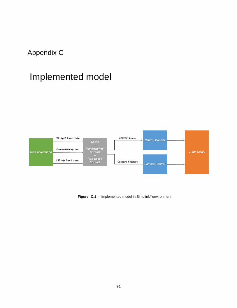
91
C. Appendix C
Appendi x A: Implemented model
Figure 0.2 C.1 - Implemented model in Simulink® environment