Development of a Freight System Conceptualization and Impact Assessment (Fre-SCANDIA) Framework

August 2018 A Research Report from the National Center for Sustainable Transportation

Miguel Jaller, University of California, Davis

John Harvey, University of California, Davis

Sogol Saremi, University of California, Davis

Hanjiro Ambrose, University of California, Davis

Ali Butt, University of California, Davis

About the National Center for Sustainable Transportation

The National Center for Sustainable Transportation is a consortium of leading universities committed to advancing an environmentally sustainable transportation system through cutting-edge research, direct policy engagement, and education of our future leaders. Consortium members include: University of California, Davis; University of California, Riverside; University of Southern California; California State University, Long Beach; Georgia Institute of Technology; and University of Vermont. More information can be found at: ncst.ucdavis.edu.

Disclaimer

The contents of this report reflect the views of the authors, who are responsible for the facts and the accuracy of the information presented herein. This document is disseminated under the sponsorship of the United States Department of Transportation’s University Transportation Centers program, in the interest of information exchange. The U.S. Government and the State of California assumes no liability for the contents or use thereof. Nor does the content necessarily reflect the official views or policies of the U.S. Government and the State of California. This report does not constitute a standard, specification, or regulation. This report does not constitute an endorsement by the California Department of Transportation (Caltrans) of any product described herein.

Acknowledgments

This study was funded by a grant from the National Center for Sustainable Transportation (NCST), supported by USDOT and Caltrans through the University Transportation Centers program. The authors would like to thank the NCST, USDOT, and Caltrans for their support of university-based research in transportation, and especially for the funding provided in support of this project.

Development of a Freight System Conceptualization and Impact Assessment

(Fre-SCANDIA) Framework A National Center for Sustainable Transportation Research Report

August 2018

Miguel Jaller, Institute of Transportation Studies, University of California, Davis

John Harvey, Department of Civil and Environmental Engineering, University of California, Davis

Sogol Saremi, Institute of Transportation Studies, University of California, Davis

Hanjiro Ambrose, Institute of Transportation Studies, University of California, Davis

Ali Butt, Institute of Transportation Studies, University of California, Davis

[page left intentionally blank]

i

TABLE OF CONTENTS

EXECUTIVE SUMMARY .....................................................................................................................1

I. Introduction and Background .......................................................................................................2

II. Brief Overview of the Freight Transportation System .................................................................4

III. Supply Chain Management .........................................................................................................7

Supply Chain Components ......................................................................................................8

Supply Chain Models and Classification Systems ...................................................................9

Supply Chain Performance Measures and Decision Variables ............................................ 12

IV. Life-Cycle Assessment .............................................................................................................. 14

Attributional and Consequential LCA .................................................................................. 17

Uncertainties in LCA ............................................................................................................. 19

Summary .............................................................................................................................. 20

V. Impact Assessment Methodologies.......................................................................................... 36

Environmental Impact Assessment (EIA) Methodologies ................................................... 36

Economic Cost-Benefit Analysis (CBA) ................................................................................. 39

Summary .............................................................................................................................. 45

VI. Freight System Conceptualization and Impact Asses Framework........................................... 63

Data Availability ................................................................................................................... 71

Models Availability ............................................................................................................... 72

VII. Framework Implementation ................................................................................................... 73

Freight Flows Data ............................................................................................................... 73

Life Cycle Inventory Data ..................................................................................................... 82

Impact Categories ................................................................................................................ 86

VIII. Case Studies ........................................................................................................................... 92

Freight Flows in California ................................................................................................... 92

Computers and Electronics Manufacturer’s Supply Chain ................................................ 114

Food Producer’s Supply Chain ........................................................................................... 121

Apparel/Shoes Manufacturer’s Supply Chain .................................................................... 129

Company’s Summary and LCA Analyses ............................................................................ 135

IX. Conclusions ............................................................................................................................ 139

X. References .............................................................................................................................. 142

ii

ANNEX ......................................................................................................................................... 150

Annex A: LCA Databases and Tools .................................................................................... 150

Annex B: LCIA Methods ..................................................................................................... 151

Annex C: CAL-B/C ............................................................................................................... 159

iii

LIST OF TABLES

Table 1. Modeling Objectives ....................................................................................................... 10

Table 2. Supply Chain Attributes................................................................................................... 11

Table 3. Performance Measures in Supply Chain Modeling ......................................................... 13

Table 4. Evolution of LCA .............................................................................................................. 14

Table 5. LCA Boundaries ............................................................................................................... 16

Table 6. Strengths and Weaknesses of Environmental LCA ......................................................... 21

Table 7. LCA Studies and Their Characteristics According to LCA Phases .................................... 22

Table 8. Classification of LCA Studies............................................................................................ 31

Table 9. Characterization Models for Impact Assessment ........................................................... 38

Table 10. Cost and Benefit Analysis .............................................................................................. 39

Table 11. Categories of Benefits from Environmental Policies .................................................... 40

Table 12. Modeling Approaches for Life Cycle Assessment and Supply Chain Management ...... 45

Table 13. Classification of Studies According to Impact Assessment Categories ......................... 47

Table 14. Freight Life Cycles .......................................................................................................... 66

Table 15. Data Availability ............................................................................................................ 71

Table 16. Industries Included in the CFS ....................................................................................... 73

Table 17. Commodities Transported ............................................................................................ 74

Table 18. Transportation Modes in the CFS ................................................................................. 76

Table 19. LCI Examples for Truck Freight Transport Processes .................................................... 84

Table 20. EMFAC 2012 Vehicle Population ................................................................................... 85

Table 21. Adjusted EURO Standard Fleet Composition ................................................................ 86

Table 22. TRACI Impact Categories ............................................................................................... 87

Table 23. TRACI Impacts for the Different Modes ........................................................................ 88

Table 24. DELL's Supply Chain Attributes ................................................................................... 116

Table 25. Global PC Market Shares ............................................................................................. 117

Table 26. DELL'S Worldwide Market Share (2011-2017) ............................................................ 117

Table 27. PC Unit Shipments in the U.S. - DELL's Quarterly Market Share 2010-2016 .............. 118

Table 28. GDP NAICS 334 Computer and Electronic Product Manufacturing (Millions of Dollars) .................................................................................................................................. 119

Table 29. Nestlé’s Supply Chain Attributes ................................................................................. 124

Table 30. Nestlé Brands in the U.S. ............................................................................................. 125

Table 31. Sales of the Leading Vendors of Chocolate Candy in the United States 2017............ 126

iv

Table 32. U.S. Market Share of Leading Chocolate Companies 2017......................................... 126

Table 33. U.S. Confectionery Market Share in 2017 ................................................................... 126

Table 34. Nestlé NIACS Subcategories ........................................................................................ 127

Table 35. GDP by Industry (Millions of Dollars) .......................................................................... 128

Table 36. Nike's Supply Chain Structure ..................................................................................... 132

Table 37. Forecast of Nike's Global Market Share in Athletic Footwear from 2011 to 2024 ..... 133

Table 38. Market Share of Leading Brand Apparel Companies in the United States in 2016 .... 133

Table 39. NICS 339 Subcategories............................................................................................... 134

Table 40. GDP by Industry (Millions of Dollars) .......................................................................... 134

Table 41. NICS 315AL Subcategories........................................................................................... 135

Table 42. GDP by Industry (Millions of Dollars) .......................................................................... 135

Table 43. Summary Market Shares and Commodities Associated to the Companies ............... 136

Table 44. Comparative Impacts per Mode for All California Flows ............................................ 140

Table 45. Comparative Assessment of Impacts Across Vehicle Types and Modes .................... 141

Table 46. Summary of Databases and Tools ............................................................................... 150

v

LIST OF FIGURES

Figure 1. Supply Chain Process ....................................................................................................... 7

Figure 2. Single Echelon .................................................................................................................. 8

Figure 3. Multi Echelon ................................................................................................................... 9

Figure 4. Life Cycle Stages ............................................................................................................. 15

Figure 5. LCA Studies Classifications According to Phases ........................................................... 30

Figure 6. LCA Studies Classifications According to Uncertainties and Risk Factors ...................... 35

Figure 7. UNITE-DSS Model Framework ....................................................................................... 43

Figure 8. California Intrastate LCA results .................................................................................... 44

Figure 9. Dollar Value on the Air-pollution Effects of a Highway Project ..................................... 45

Figure 10. Classification of Studies According to Impact Assessment Factors ............................. 62

Figure 11. Logical Framework ....................................................................................................... 64

Figure 12. Goal and Scope ............................................................................................................ 65

Figure 13. Examples of Services to Consider in Freight LCA ......................................................... 67

Figure 14. Defining Measurement Indicators, Data Collection, Impact Assessment Categories, and Analysis of Results ......................................................................................................... 70

Figure 15. Ton-miles Originated from (Out) and Destined to (In) California in 2012 per Industry Sector per Mode of Transport ............................................................................................. 78

Figure 16. Comparative Mode Share for Ton-miles Originated from (Out) and Destined to (In) California in 2012 per Industry Sector ................................................................................. 79

Figure 17. Ton-miles Originated from (Out) and Destined to (In) California in 2012 per Commodity Group per Mode of Transport.......................................................................... 80

Figure 18. Comparative Mode Share for Ton-miles Originated from (Out) and Destined to (In) California in 2012 per Commodity Group ............................................................................ 81

Figure 19. EURO Shares for Different Vehicles Types ................................................................... 85

Figure 20. Ecotoxicity and Human Toxicity per Ton-Km ............................................................... 89

Figure 21. GWP, Human Particles, and Ozone Depletion Potential per Ton-Km ......................... 90

Figure 22. Smog, Acidification and Eutrophication Impacts per Ton-Km ..................................... 91

Figure 23. Ecotoxicity Impacts from All California Flows (top) and Average per Ton-km (bottom) for each Industry Category .................................................................................................. 94

Figure 24. Human Health Cancer Impacts from All California Flows (top) and Average per Ton-km (bottom) for each Industry Category ............................................................................. 95

Figure 25. Human Health Non-Cancer Impacts from All California Flows (top) and Average per Ton-km (bottom) for each Industry Category...................................................................... 96

vi

Figure 26. Global Warming Potential Impacts from All California Flows (top) and Average per Ton-km (bottom) for each Industry Category...................................................................... 97

Figure 27. Human Health Particulate Impacts from All California Flows (top) and Average per Ton-km (bottom) for each Industry Category...................................................................... 98

Figure 28. Ozone Depletion Potential Impacts from All California Flows (top) and Average per Ton-km (bottom) for each Industry Category...................................................................... 99

Figure 29. Photochemical Smog Formation Potential Impacts from All California Flows (top) and Average per Ton-km (bottom) for each Industry Category ............................................... 100

Figure 30. Acidification Potential Impacts from All California Flows (top) and Average per Ton-km (bottom) for each Industry Category ........................................................................... 101

Figure 31. Eutrophication Potential Impacts from All California Flows (top) and Average per Ton-km (bottom) for each Industry Category ........................................................................... 102

Figure 32. California Flow Total TRACI Impacts .......................................................................... 104

Figure 33. Ecotoxicity Impacts from All California Flows (top) and Average per Ton-km (bottom) for each Commodity Group ............................................................................................... 105

Figure 34. Human Health Cancer Impacts from All California Flows (top) and Average per Ton-km (bottom) for each Commodity Group .......................................................................... 106

Figure 35. Human Health Non-Cancer Impacts from All California Flows (top) and Average per Ton-km (bottom) for each Commodity Group .................................................................. 107

Figure 36. Global Warming Potential Impacts from All California Flows (top) and Average per Ton-km (bottom) for each Commodity Group .................................................................. 108

Figure 37. Human Health Particulate Impacts from All California Flows (top) and Average per Ton-km (bottom) for each Commodity Group .................................................................. 109

Figure 38. Ozone Depletion Potential Impacts from All California Flows (top) and Average per Ton-km (bottom) for each Commodity Group .................................................................. 110

Figure 39. Photochemical Smog Formation Potential Impacts from All California Flows (top) and Average per Ton-km (bottom) for each Commodity Group .............................................. 111

Figure 40. Acidification Potential Impacts from All California Flows (top) and Average per Ton-km (bottom) for each Commodity Group .......................................................................... 112

Figure 41. Eutrophication Potential Impacts from All California Flows (top) and Average per Ton-km (bottom) for each Commodity Group .......................................................................... 113

Figure 42. DELL World Map ........................................................................................................ 114

Figure 43. U.S. Map for DELL ...................................................................................................... 115

Figure 44. DELL's Supply Chain ................................................................................................... 115

Figure 45. Industries by their Value of Shipments ...................................................................... 121

Figure 46. Nestlé World Map ...................................................................................................... 122

Figure 47. U.S. Map for Nestlé .................................................................................................... 122

vii

Figure 48. Nestlé Supply Chain ................................................................................................... 123

Figure 49. Nike World Map ......................................................................................................... 130

Figure 50. U.S. Map for Nike ....................................................................................................... 130

Figure 51. Nike Supply Chain ...................................................................................................... 131

Figure 52. Inbound & Outbound Total Shipments per Mode (top) and Mode Share (bottom) . 137

Figure 53. Average TRACI Impact per Ton-km) for each Company ............................................ 138

Figure 54. IMPACT 2002+ Methodology Impact Category ......................................................... 152

Figure 55. CML Methodology Impact Categories ....................................................................... 153

Figure 56. Eco-indicator 99 Methodology Impact Categories .................................................... 154

Figure 57. LIME Methodology Impact Category ......................................................................... 155

Figure 58. LUCAS Methodology Impact Category....................................................................... 156

Figure 59. ReCiPe Methodology Impact Category ...................................................................... 157

Figure 60. EDIP Methodology Impact Category .......................................................................... 158

Figure 61. CAL-B/C Components ................................................................................................. 159

Figure 62. CAL-B/C Emissions Calculator .................................................................................... 160

1

Development of a Freight System Conceptualization AND Impact Assessment (Fre-SCANDIA) Framework

EXECUTIVE SUMMARY

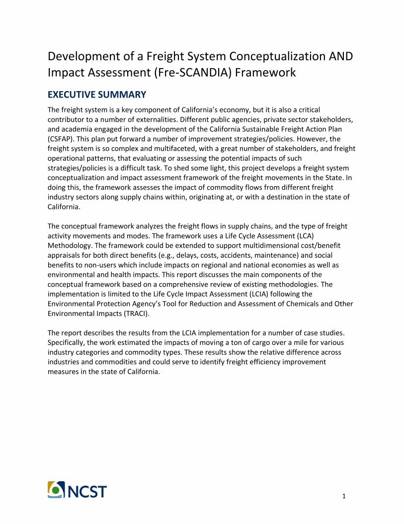
The freight system is a key component of California’s economy, but it is also a critical contributor to a number of externalities. Different public agencies, private sector stakeholders, and academia engaged in the development of the California Sustainable Freight Action Plan (CSFAP). This plan put forward a number of improvement strategies/policies. However, the freight system is so complex and multifaceted, with a great number of stakeholders, and freight operational patterns, that evaluating or assessing the potential impacts of such strategies/policies is a difficult task. To shed some light, this project develops a freight system conceptualization and impact assessment framework of the freight movements in the State. In doing this, the framework assesses the impact of commodity flows from different freight industry sectors along supply chains within, originating at, or with a destination in the state of California. The conceptual framework analyzes the freight flows in supply chains, and the type of freight activity movements and modes. The framework uses a Life Cycle Assessment (LCA) Methodology. The framework could be extended to support multidimensional cost/benefit appraisals for both direct benefits (e.g., delays, costs, accidents, maintenance) and social benefits to non-users which include impacts on regional and national economies as well as environmental and health impacts. This report discusses the main components of the conceptual framework based on a comprehensive review of existing methodologies. The implementation is limited to the Life Cycle Impact Assessment (LCIA) following the Environmental Protection Agency’s Tool for Reduction and Assessment of Chemicals and Other Environmental Impacts (TRACI). The report describes the results from the LCIA implementation for a number of case studies. Specifically, the work estimated the impacts of moving a ton of cargo over a mile for various industry categories and commodity types. These results show the relative difference across industries and commodities and could serve to identify freight efficiency improvement measures in the state of California.

2

I. Introduction and Background

California has the largest State economy in the U.S. and is a major supplier of agricultural and high-tech manufactured products for the rest of the nation (Viljoen et al., 2014). The State’s freight transportation system is critical to California’s economy and to the economies of other States–20 percent of all U.S. foreign trade passes through California (California Department of Transportation, 2014). However, the vehicles, equipment, and facilities used by the different economic agents that conduct these freight operations generate a great deal of externalities including congestion, environmental emissions, and safety issues, among other impacts (Regan and Golob, 1999; Holguín-Veras et al., 2015; Jaller et al., 2016a). For example, freight accounts for about half of toxic diesel particulate matter (diesel PM), 45 percent of the emissions of nitrogen oxides (NOx) that form ozone and fine particulate matter in the atmosphere, and six percent of the greenhouse gas (GHG) emissions in California (California Air Resources Board, 2015). These statistics, however, only include emissions from vehicles and the equipment used to move freight at seaports, airports, railyards, warehouses and distribution centers. The actual impacts from freight, including the necessary infrastructure, could be much higher. Different operational patterns, seasonality, lack of freight data, the multiplicity of economic agents, diverse supply chain structures and their interactions difficult the understanding of the freight system (Holguín-Veras and Jaller, 2014). These factors make the actual estimation of the full impacts a complex task (Jaller et al., 2016b). At the same time, public agencies are developing policies and methodologies to minimize the negative impacts of the system, while trying to maximize its benefits. In order to take these policies from well-intentioned to effective, there is an urgent need to be able to evaluate the impacts of the freight transportation system (considering the supply chains that move the goods and services required for this vibrant economy). This requires the understanding and availability of a system conceptualization that characterizes the components and structural forms of the key types of supply chains active in the State, whether the policies are evaluated under horizontal or vertical equity considerations (Litman, 2009; Litman, 2016). However, the freight system is so diverse that there could be a sheer number of inputs and outputs, thus defining a common measure to evaluate the system would be problematic (Barber and Grobar, 2001). Most supply chains are distributive networks, while others are performed in spoke and wheel patterns or corridors; some are defined within the boundaries of the state while others transcend its geographical and political limits (Rodrigue, 2013; SCAG, 2016). In some cases, products consumed, transformed, or exported in the State, may have already entered and exited the boundaries several times. Whilst some flows of cargo pass through urban areas, others have the urban areas as the destination. Therefore, evaluating the components inside the State or within specific geographic locations could foster some overall inefficiencies in the system. This is because supply chain optimization may be achieved when looking at the holistic chain/system, and not, when only optimizing specific components. Within the system, numerous market forces affect the way each individual player performs and their roles; each subset of each supply chain aims to maximize its own utility and efficiency, and to

3

minimize its own cost of doing business. Consequently, having each individual player maximizing its own efficiency does not guarantee achieving system optimum. The objective of this research is to help fill this gap by developing a Freight System Conceptualization AND Impact Assessment (Fre-SCANDIA) Framework of the freight movements in the State. The framework analyzes the main transportation flows of key supply chains and serves as an impact assessment tool. The framework can help identify the industry sector, or the commodity types that have the largest impacts, and potentially identify which economic agents’ decisions or regulatory actions affect a particular impact category the most. The framework, and the results discussed in this report can help agencies develop and understand appropriate performance measures by providing a methodology to estimate the baseline impacts of freight activity. To achieve the objective, the research team developed a conceptual framework based on a Life Cycle Assessment (LCA) methodology considering the movement of goods within supply chains in different industries. The proposed LCA-based framework could be modified to support multidimensional cost/benefit appraisals for both direct benefits (e.g., delays, costs, accidents, maintenance) and social benefits to non-users as well as environmental and health impacts. The team conducted a number of case studies on different economic sectors and specific companies to illustrate the framework implementation and identify current methodological, data, and modeling gaps. This report discusses the results of the research and contains the following sections. Section II provides a brief overview of the freight system, concentrating on the various modes of transport. Section III discusses key concepts from supply chain management that are important for the development of the proposed framework. Considering that the conceptual framework uses the LCA structure as a basis, Section IV is a comprehensive review of the state of practice of LCA. Section V discusses a wide range of impact assessment methodologies that range from general impact assessment tools, to specific environmentally- or economically-focused methods. Section VI reviews LCA implementations in transportation and the relationship with supply chain assessments. Section VII puts forward the Fre-SCANDIA framework. This section discusses the data and methodological gaps in the literature, which would be required for the development and implementation of the framework. Section VIII describes the basic implementation of the framework limited to the LCIA of freight flows. The section discusses a number of case studies. These include DELL as a leading computer hardware company; Nestlé as one of the largest food supply chains around the world; and, Nike for its distinct third party logistics. The research team selected these case studies because of their representation of different industries and scope, and more importantly because of data availability to support modeling assumptions.

4

II. Brief Overview of the Freight Transportation System

Freight or cargo are the products or goods transported, usually for commercial benefit. The transport of goods can be done through a different set of modes: air, land (truck, rail), and water. However, besides the typical consideration of freight as the cargo itself, the freight system can also be understood as the movement of those cargoes; and, it could also be defined not only in terms of the commodity weight or value, but as the number of shipment and resulting vehicle trips generated (National Research Council, 2012). Usually, freight was associated with the large movement of break-bulk or containerized cargo, through large freight vehicles. It is now common to include in the freight definition, the movement of express, household goods, parcel, and other products that span the combinations of business and consumer interactions (Fitzpatrick et al., 2016). Overall, the freight transportation system is a complex system of systems, where a multiplicity of agents conduct a wide range of commercial activities related to a large number of commodities, services, or other economic transactions through different modes, vehicles, and operational strategies (Lamm et al., 2017). In freight transportation, there are a number of terms that may have different understandings. For instance, while shipping may be associated with the action of sending-out goods by a “shipper” agent, shipping is also a general term originally used to refer to transport of goods by sea (Talley, 2014). The infrastructure and the companies (carriers) that move the goods support the supply of freight transportation. Receivers or consumers of the cargo could be the final consumption point or an intermediary destination that can transform the goods (Holguín-Veras and Jaller, 2014). Freight infrastructure includes the roadway system, railroads, airports, marine ports, locks and dams on rivers, pipelines, and other facilities such as warehouses, distribution centers, and intermodal yards, among others. In the U.S, the National Highway System (NHS) contains approximately 160,000 miles of the roads directly affecting the national economy and mobility (Rondinelli and Berry, 2000). The total road network in the US accounts for about 2.7 million miles of paved roads, and an additional 1.3 million miles of unpaved roads. Freight carriers are the owners or operators of the trucks, trains, ships, and airplanes that provides transportation to shippers. Other important private players in freight transportation include freight brokers, freight forwarders, and third-party logistics providers. Freight brokers assist shippers and carriers in assembling paperwork for international or complicated shipments. Freight forwarders consolidate multiple small shipments into larger shipments for transport (ICF International et al., 2011). The reader is referred Holguín-Veras et al. (2012) for a detailed description of agents’ characteristics and interactions. Cargo characteristics determine the type of transportation service demanded by shippers. Companies shipping high-value or perishable cargo tend to select truck or air transport to reduce transit time and gain higher levels of reliability. Airfreight carries high-value goods for which delivery within a few hours is often critical, such as express parcels and fresh flowers. Passenger and freight-only air carriers transport goods. Large freight-only carriers include Atlas Air, ASTAR Air Cargo, and Polar Air Cargo (Rondinelli and Berry, 2000). In the U.S., there are nearly 171,000 miles of railroad and hundreds of yards to assemble or dissemble the trains. Rail usually transports lower value, slow-moving bulk cargo, coal and other high-volume cargo

5

through longer distances (more than 200-300 miles), thus it is popular for refineries, coal, and other large manufacturers. Trucks move a range of products, but they move a greater percent of higher value commodities like finished consumer products, computers, and pharmaceuticals (Bell and Iida, 1997). Domestic marine transport tends to carry low-value bulk cargo for which speed is not an important factor. Pipelines primarily transport petroleum products and natural gas. The length of haul is also an important shipment characteristic that determines mode choice. Trucks tend to carry a larger percentage of short-haul movements. Trucking services can also be private or for-hire. Private services or private carriers are those that use their own fleets to move their cargoes. On the hand, for-hire carriers offer their services to the open market. In the private sector, large companies such as Coca-Cola, Walmart, and Safeway, tend to use private fleets to move their cargo and maintain the reliability of service. Truck Load (TL) services provide truck transport to move cargo throughout the nation, while Less-than-Truck-Load (LTL) services move smaller shipments at the local level. These types of services can also incorporate consolidation of shipments, or can carry shipments to a specific terminals to be moved to their final destination (Crainic, 2003). Yellow Roadway, ABF, Con-way, Old Dominion Freight, FedEx Freight, and UPS Freight are examples of the largest U.S national LTL carriers. The network of LTL services requires terminals throughout the routes. Rail, ocean, and air shipments tend to have a longer average shipment distance. Freight shipments often use more than a single mode of transportation. Trucks connect shippers to rail or maritime transportation modes or provide the “last mile” to the customer. “Intermodal” freight typically refers to freight moving in containers or trailers transferred between ships, railroads, and trucks. By reducing the cost of using multiple modes of transportation, intermodal freight movements allow shippers to use lower cost modes (such as rail or maritime) for long-haul movements and then switch to truck carriers to reach a final destination (Crainic, 2003). Some express carriers like Federal Express and UPS use their own multimodal transportation system to prove a door-to-door service (Rondinelli and Berry, 2000; PROTECTION, 2003). While maritime services move the bulk of the cargo using water-based modes, inland waterways also transport cargo in specific locations in the country. Finally, the pipeline system carries specific cargo, usually petroleum products and other chemicals. The pipeline system includes collection pipelines, which are those used for moving natural gas or its products, and transmission pipelines, which transport over a far distance (e.g., moving natural gas to distant power plants, factories or distribution center). Additionally, the distribution lines, which move cargos like natural gas in shorter distances (Ganeshan and Harrison, 1995). Although describing the system in terms of the cargo, modes, and the individual economic agents is important, the reality is that most of these economic agents comprise a number of supply chains. Some of these supply chains integrate the decision-making process, while others have independent agents. Nevertheless, understanding the freight system requires knowledge about supply chain structures, logistics, and management. In general, freight transportation

6

results from economic and logistics decisions. Economic transactions between agents translate into the physical movement of the cargo, but the ultimate decisions of the mode, shipment size, vehicle size, and frequency of delivery come from logistics and supply chain management processes.

7

III. Supply Chain Management

A holistic supply chain includes processes and procedures to extract raw material, transport them to manufacturing facilities, produce final products, and distribute them to the consumers (wholesale or retail). Consequently, there are different stockholders involved such as suppliers, manufacturers, distributers, and retailers, among others. Supply chains flows include forward and reverse physical (e.g., returns), and information flows (Stadtler, 2005). At its highest level, a supply chain is comprised of two basic and integrated processes:

▪ The production planning and inventory control process; and,

▪ The distribution and logistics process.

The production planning and inventory control (first phase) consists of processes to gather raw materials and finally transform them into the final (or intermediary) products. Inventory control is embed into the manufacturing planning process and affects the procurement of raw material, defines the ordering schedule, and is part of the design and control of processes and products (Stadtler, 2005). The second phase determines the products’ distribution among wholesalers, retailers, or the final consumer. That is, the distribution process determines the transportation of goods directly to retailers, or transporting all the cargo to a wholesaler or a facility in order to distribute them among retailers. According to these process, a supply chain can include all or some parts of these activities which define the specific structure of the supply chain (Beamon, 1998). For instance, Figure 1 shows a supply chain configuration involving five stages.

Figure 1. Supply Chain Process (Beamon, 1998) Broadly, Supply Chain Management (SCM) focuses on the required processes to manage the supply chains. SCM includes decisions and evaluations at different levels and needs. Traditionally, the objective of SCM was to be cost effective across the whole system, including the transportation systems, inventory and raw material management, as well as finished goods and products. However, in recent years, the introduction of sustainable SCM considers other criteria such as social acceptability, efficiency, and environmentally beneficial aspects. Although there have been many methodological and technical advances during the last century, studying a supply chain is still a challenging task and there are multiple reasons for it. The study of supply

8

chains usually focuses on specific products or services, as there are many interconnected dimensions as well as upstream and downstream supply chains. Designing and operating a supply chain needs to be cost-effective, thus requiring a service-level that guarantees the profitability of the business. Moreover, there are inherent uncertainty, risks, and disruptions that threaten supply chains.

Supply Chain Components

Manufacturing

Manufacturing refers to all the processes and facilities required to change the raw materials into intermediate or final products. Manufacturing facilities vary according to the number and type of their production processes.

Inventory

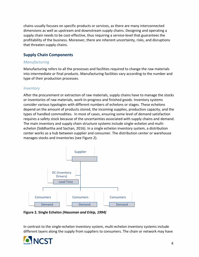
After the procurement or extraction of raw materials, supply chains have to manage the stocks or inventories of raw materials, work-in-progress and finished goods. Inventory systems consider various typologies with different numbers of echelons or stages. These echelons depend on the amount of products stored, the incoming supplies, production capacity, and the types of handled commodities. In most of cases, ensuring some level of demand satisfaction requires a safety stock because of the uncertainties associated with supply chains and demand. The main inventory and supply chain structure systems include single-echelon and multi-echelon (Siddhartha and Sachan, 2016). In a single echelon inventory system, a distribution center works as a hub between supplier and consumer. The distribution center or warehouse manages stocks and inventories (see Figure 2).

Figure 2. Single Echelon (Hausman and Erkip, 1994) In contrast to the single-echelon inventory system, multi-echelon inventory systems include different layers along the supply from suppliers to consumers. The chain or network may have

Supplier

Consumers

Demand

Consumers

Demand

Consumers

Demand

DC (Inventory Drivers)

Lead Time

9

different distribution centers connecting suppliers to consumers. In a typical multi-echelon system, a central warehouse stores all the cargo; from there, the cargo goes to various smaller distribution facilities connected to the retailers and consumers (Figure 3). Many supply chains with multi-echelon inventory systems implement a hierarchical design with some regional larger distribution centers and some smaller facilities that service end customers. For instance, Nike as one of the biggest supply chains around the world, distributes its products into seven major regional distribution centers and from there products send to different retailers (Sanyai, January 28, 2014).

Figure 3. Multi Echelon (Hausman and Erkip, 1994)

Assembly and Distribution

Assembly takes place in supply chains with multi-echelon manufacturing systems in which parts from different suppliers comes to one place to finalize the product. For examples, the assembly of electronic devices happens at one place where the different parts coming from several sources merge. In these supply chains, the scheduling has a huge impact on the inventory level as well as the product distribution. A multi-echelon supply chain needs to manage the inventory in terms of fill orders and lead-time. These types of supply chain can maintain very high or very low operation and inventory cost depending on their service to their downstream supply chains. Strategies such as Just-in-Time (JIT) can have important implications for the inventory and distribution process (Whatis, 2014). In general, JIT have reduced inventory levels along supply chains; though have increased the frequency of distribution (resulting in more vehicle trips, and smaller shipments).

Supply Chain Models and Classification Systems

Generally, there are four main categories of supply chain models based on the modeling approach, the nature of the inputs and the objective of the study. The reader is referred to Beamon (1998) for a detailed description of these models:

Supplier

Consumers

Demand

Consumers

Demand

Consumers

Demand

DC (Inventory Drivers)

Lead Time

RDC Inventory Drivers)

Lead Time

10

▪ Deterministic analytical models;

▪ Stochastic analytical models;

▪ Economic models, and

▪ Simulation models.

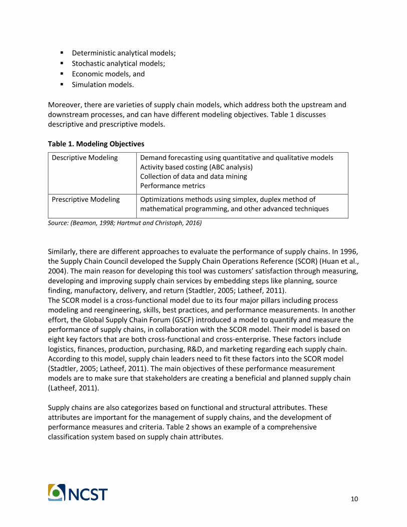
Moreover, there are varieties of supply chain models, which address both the upstream and downstream processes, and can have different modeling objectives. Table 1 discusses descriptive and prescriptive models. Table 1. Modeling Objectives

Descriptive Modeling Demand forecasting using quantitative and qualitative models Activity based costing (ABC analysis) Collection of data and data mining Performance metrics

Prescriptive Modeling Optimizations methods using simplex, duplex method of mathematical programming, and other advanced techniques

Source: (Beamon, 1998; Hartmut and Christoph, 2016)

Similarly, there are different approaches to evaluate the performance of supply chains. In 1996, the Supply Chain Council developed the Supply Chain Operations Reference (SCOR) (Huan et al., 2004). The main reason for developing this tool was customers’ satisfaction through measuring, developing and improving supply chain services by embedding steps like planning, source finding, manufactory, delivery, and return (Stadtler, 2005; Latheef, 2011). The SCOR model is a cross-functional model due to its four major pillars including process modeling and reengineering, skills, best practices, and performance measurements. In another effort, the Global Supply Chain Forum (GSCF) introduced a model to quantify and measure the performance of supply chains, in collaboration with the SCOR model. Their model is based on eight key factors that are both cross-functional and cross-enterprise. These factors include logistics, finances, production, purchasing, R&D, and marketing regarding each supply chain. According to this model, supply chain leaders need to fit these factors into the SCOR model (Stadtler, 2005; Latheef, 2011). The main objectives of these performance measurement models are to make sure that stakeholders are creating a beneficial and planned supply chain (Latheef, 2011). Supply chains are also categorizes based on functional and structural attributes. These attributes are important for the management of supply chains, and the development of performance measures and criteria. Table 2 shows an example of a comprehensive classification system based on supply chain attributes.

11

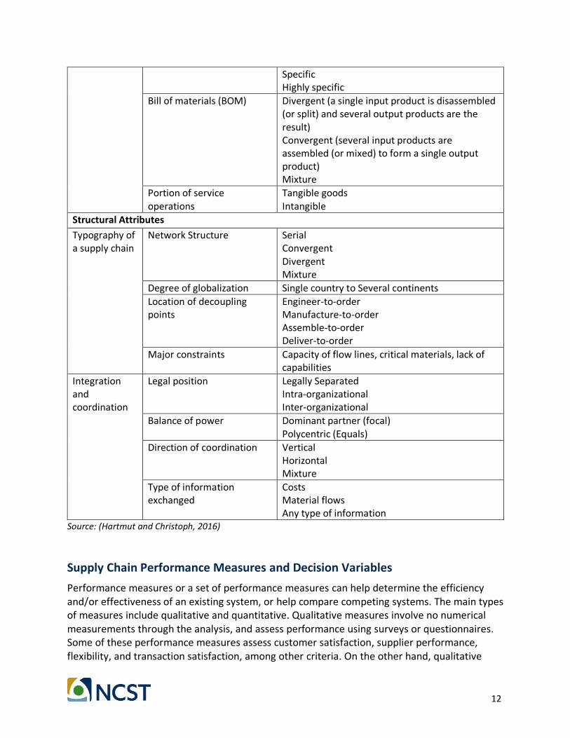
Table 2. Supply Chain Attributes

Functional attributes

Procurement Type

Number and type of products procured

Few Many

Sourcing type Single Double Multiple

Suppliers’ flexibility (Amounts to be supplied)

Low High

Supplier lead time and reliability

Short (More reliable) Long (Less reliable)

Material’s life cycle Short Long

Production Type

Organization of the production process

Flow shop Job shop

Repetition of operations Mass production Batch production One-of-a-kind Products

Changeover characteristics Fixed Sequence dependent

Bottlenecks in production Stationary and known Shifting

Working time flexibility Single shifts Multiple shifts

Distribution Type

Distribution structure One-stage (one link between warehouse and customers) Two-stage (one intermediate layer, e.g. having central warehouse (CW) or regional warehouse (RW)) Three stage

Pattern of delivery Cyclic (fixed interval times) Dynamic (demand dependent)

Deployment of transportation means

Routes (Standards, variable) Capacity (limited, unlimited) Loading requirement (full truck load, …)

Distribution Type

Availability of future demands

Unforeseen Forecasted

Demand curve Seasonal Sporadic Static

Product’s life cycle Number of days, months, years

Number of product types Few Many

Degree of customization Standard

12

Specific Highly specific

Bill of materials (BOM) Divergent (a single input product is disassembled (or split) and several output products are the result) Convergent (several input products are assembled (or mixed) to form a single output product) Mixture

Portion of service operations

Tangible goods Intangible

Structural Attributes

Typography of a supply chain

Network Structure Serial Convergent Divergent Mixture

Degree of globalization Single country to Several continents

Location of decoupling points

Engineer-to-order Manufacture-to-order Assemble-to-order Deliver-to-order

Major constraints Capacity of flow lines, critical materials, lack of capabilities

Integration and coordination

Legal position Legally Separated Intra-organizational Inter-organizational

Balance of power Dominant partner (focal) Polycentric (Equals)

Direction of coordination Vertical Horizontal Mixture

Type of information exchanged

Costs Material flows Any type of information

Source: (Hartmut and Christoph, 2016)

Supply Chain Performance Measures and Decision Variables

Performance measures or a set of performance measures can help determine the efficiency and/or effectiveness of an existing system, or help compare competing systems. The main types of measures include qualitative and quantitative. Qualitative measures involve no numerical measurements through the analysis, and assess performance using surveys or questionnaires. Some of these performance measures assess customer satisfaction, supplier performance, flexibility, and transaction satisfaction, among other criteria. On the other hand, qualitative

13

measures use numerical methods to assess the performance (e.g., costs and benefits, customer’s responsiveness) of supply chains. Cost-based measures include sales, profits, return on investments, operational costs, and inventory levels. Evaluation of responsiveness of customers can be through defining certain factors, which are dependent on the manufacture, inventory and distribution processes of the supply chain. These measures can be the lead-time of the distribution, lateness in deliveries, and customer response time (Marco Montorio, 2007). Beamon (1998) proposes eight categories for the decision variables: inventory levels; number of echelons; production and distribution scheduling; distribution centers; number of product types held in inventory; relationships with suppliers; product differentiation; and, product assignment. Moreover, the author lists several performance measures with different focus criteria (see Table 3). Just until recently, performance measures did not include factors that were not direct impacts to the environment, even when other authors have defined a supply chain as “product life cycle processes comprising physical, information, financial, and knowledge flows whose purpose is to satisfy end-user requirements with physical products and services from multiple, linked suppliers” (Ayers, 2006). Table 3. Performance Measures in Supply Chain Modeling

Basis Performance Measures

Cost Minimize cost Minimize average inventory levels Maximize profit Minimize amount of obsolete inventory

Customer Achieve target service level

Responsiveness Minimize stock out probability

Cost and customer responsiveness Minimize product demand variance or demand amplification Maximize buyer-supplier benefit

Cost and activity time Minimize the number of activity days and total cost

Flexibility Maximize available system capacity Source: (Beamon, 1998)

14

IV. Life-Cycle Assessment

The study of Life Cycle Assessment (LCA) began with the launch of the environmental Acts in 1970s. The Coca-Cola Company was the first one to study this concept to evaluate the environmental impact of containers in 1969. By that time, increasing concerns regarding resource availability and energy use highlighted the need for studies to measure the environmental impacts of processes and products (Curran, 1993; Dicks and Hent, 2014). After the initial studies (mostly by the Midwest Research Center), other institutes such as Battelle Frankfurt, EMPA in Switzerland and Sundström in Sweden, approached the topic. Early studies considered environmental dimensions regarding product packaging (Hunt et al., 1996a). Before the current LCA denomination, the studies were called resource and profile analysis (REPA) (Hunt et al., 1996b). In 2000, researchers started to investigate the similarities and differences between LCA and Partial model equilibrium (PE) models used to evaluate the effect of a policy on a specific market (Bouman et al., 2000; Guinée et al., 2001). Most of the partial equilibrium (PE) models concerns Multi-Market, Multi-Region Partial Equilibrium Models. Nevertheless, the Coca-Cola study set LCA as a tool for assessing environmental impacts. Furthermore, other initial experiences defined LCA as a toll for evaluating complex systems and a sustainability measure tool of products, processes, and companies. Table 4 briefly lists the evolution of LCA (Guinee et al., 2010). Table 4. Evolution of LCA

The evolution of LCA is divided into four eras (Guinee et al., 2010) ▪ 1970-1990: “Decades of Conception”

“…Due to the increased awareness and public concerns regarding the pollutions, solid

wastes, resources and energy efficiency, the first studies of LCA were conducted in late

1960s”.

▪ 1990-2000: “Decade of Standardization”

“…Through this era, which is known for coordination of scientific activities around the

world, a solid and holistic framework was provided both as SETAC and ISO’s perspective

for LCA studies. Through this period the main focus of LCA was packaging legislations”

(Finkbeiner et al., 2006; Normalización, 2006).

▪ 2000-2010: “Decade of Elaboration”

“..During this period, the environmental policy decisions started to be made by life cycle analysis, and even the U.S. Environmental Protection Agency started supporting the use of LCA.”

In this era, many authors proposed several ways to perform LCA studies. These methods differed with respect to the system boundary and the allocation problem (Guinee et al., 2010). For instance: ▪ Dynamic LCA,

▪ Spatially differentiated LCA,

▪ Risk-based LCA,

15

▪ Environmental input-output based LCA (EIO-LCA), and

▪ Hybrid LCA.

▪ The present day of LCA (2010-2020): Decade of Life Cycle Sustainability Analysis

In this era, the LCA studies consider all dimensions of sustainability: social, environmental and economical. The studies consider both products and sectors. Now, the Proposition of Life Cycle Sustainable Assessment (LCSA) is a framework comprised of models rather than a model itself.

Source: Adapted from (Guinee et al., 2010)

In general, a comprehensive LCA includes various stages and each directly affects the estimations and results. These stages include raw material acquisition, product manufacturing, usage and disposal, and the recycling of a product. There are different approaches for setting the boundary of the processes’ in LCA studies such as Cradle-to-Grave, Cradle-to-Gate, Gate-to-Gate, Gate-to-Grave, or Cradle-to-Cradle (see Figure 4 and Table 5).

Figure 4. Life Cycle Stages (Dicks and Hent, 2014)

Raw Material Acquisition and synthesis of starting materials

Product Synthesis

Product Usage and disposal

Recycling back into raw materials

Cradle

Cradle

Gate

Grave

Input: Energy Raw material

Output: Emissions to environment Energy Co-Product Formation Solid Waste

16

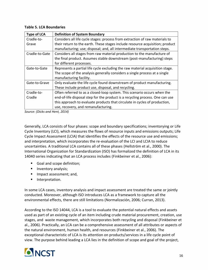
Table 5. LCA Boundaries

Type of LCA Definition of System Boundary

Cradle-to-Grave

Considers all life cycle stages: process from extraction of raw materials to their return to the earth. These stages include resource acquisition; product manufacturing; use; disposal; and, all intermediate transportation steps.

Cradle-to-Gate Considers all stages from raw material production to the manufacture of the final product. Assumes stable downstream (post-manufacturing) steps for different processes.

Gate-to-Gate Represents a partial life cycle excluding the raw material acquisition stage. The scope of the analysis generally considers a single process at a single manufacturing facility.

Gate-to-Grave Only evaluate the life cycle found downstream of product manufacturing. These include product use, disposal, and recycling.

Cradle-to-Cradle

Often referred to as a closed-loop system. This scenario occurs when the end-of-life disposal step for the product is a recycling process. One can use this approach to evaluate products that circulate in cycles of production, use, recovery, and remanufacturing.

Source: (Dicks and Hent, 2014)

Generally, LCA consists of four phases: scope and boundary specifications; inventorying or Life Cycle Inventory (LCI), which measures the flows of resource inputs and emissions outputs; Life Cycle Impact Assessment (LCIA) that identifies the effects of the resource use and emissions; and interpretation, which incorporates the re-evaluation of the LCI and LCIA to reduce uncertainties. A traditional LCA contains all of these phases (Hellström et al., 2000). The International Organization for Standardization (ISO) has formalized the definition of LCA in its 14040 series indicating that an LCA process includes (Finkbeiner et al., 2006):

▪ Goal and scope definition;

▪ Inventory analysis;

▪ Impact assessment; and,

▪ Interpretation.

In some LCA cases, inventory analysis and impact assessment are treated the same or jointly conducted. Moreover, although ISO introduces LCA as a framework to capture all the environmental effects, there are still limitations (Normalización, 2006; Curran, 2013). According to the ISO 14044, LCA is a tool to evaluate the potential natural effects and assets used as part of an existing cycle of an item including crude material procurement, creation, use stages, and waste management, which incorporates both recycling and disposal (Finkbeiner et al., 2006). Practically, an LCA can be a comprehensive assessment of all attributes or aspects of the natural environment, human health, and resources (Finkbeiner et al., 2006). The exceptional characteristic of LCA is its attention on products/services in a life cycle point of view. The purpose behind leading a LCA lies in the definition of scope and goal of the project,

17

the system boundaries, and its functional units. Quantitatively measuring the impacts of a good or service requires defining a functional unit. The outcome of the LCI is a collection of the inputs (resources) and the outputs (emissions) from the item over its life cycle in connection to the functional unit. The LCIA analyzes and assesses the magnitude and significance of the potential natural effects of the contemplated framework (Finkbeiner et al., 2006). The estimation of impacts considers specific boundary conditions with a spatial and temporal dimension. For instance, the results allow a comparison of the emissions produced in past years with the ones emitted today and the ones at some point in the future. Although much of the focus of LCA is to quantify emissions and outputs of a process, it may not fully consider the relationships and interdependencies of all the potential affected processes that fall outside the system under study. As a result, the analyses may require environmental risk assessment methodologies (Hertwich et al., 2002). Generally, LCAs require large amounts of data, and the boundary setting and scope could limit and ease such requirements. In LCA, the very first step is the planning phase that define the objectives of the LCA and the required information. This step also specifies the level of details of the study (Consoli et al., 1993). After recognizing the system boundaries, the second step in an LCA process is the inventory analysis. This phase gathers the required data regarding mass, and energy requirements, among others, and builds the flow charts according to the system boundaries. Often, the analyses use quantitative data collected or estimated from approximations, assumptions, or from the literature. With the growing interests in LCA studies, there are now databases that can provide more quantitative information for each product or material. The primary motivation behind the third phase is to evaluate the ecological effects as per the selected impact categories that may include human medical problems, air contamination, commotion contamination, sea-going poisonous quality, global warming, asset exhaustion, eutrophication, and so on. In addition, LCA could consider the social effects, costs, and other specific issues. The fourth stage requires interpreting the other stages. The fundamental explanation behind this sequential process is to introduce the ethics and scope of the proposed LCA analysis.

Attributional and Consequential LCA

Initial LCA studies focused on energy use and public environmental concerns in the 1970s. Later, in the 1980s and 1990s, LCA considered more a holistic assessment and introduced costing (McManus and Taylor, 2015). The first decade of the 21st century welcomed social LCA and the new consequential type of LCA (Guinee et al., 2010). One of the complexities regarding LCA studies is how to allocate impacts among different products, or processes. As a result, there are two common types of LCA: attributional and consequential. Attributional LCA (ALCA) considers the environmental consequences directly related to the physical flows regarding

18

single or multiple product or process, while consequential LCA (CLCA) discusses how much environmental flows change with respect to possible changes or decisions (Earles and Halog, 2011). CLCA accounts for a broader spectrum compared to ALCA. Differences between attributional and consequential LCA conditions the choice of methodology and data requirements for the LCI and LCIA phases (Finnveden et al., 2009a). LCA studies require extensive amounts of data. Consequently, in many cases, the nature of the data influences the results in both ALCA and CLCA. Usually, LCA requires information with respect to the generation costs, versatility of supply and more information according the end goal to extrapolate drifts in costs and yields (Searchinger et al., 2008; Curran, 2014). CLCA is a complex technique since it can require various economic models (Pesonen et al., 2000). Weidema (1993) was among the first to discuss CLCA, which largely emphasized the need to consider market information in LCI data and analyses. CLCA is a modeling approach with a specific goal to show environmental effects and not only the physical direct impacts from ALCA. The first efforts to combine ALCA and CLCA use PE models and other heuristic approaches. Although researchers and practitioners used multi-Market, Multi-Regional PE and Computable General Equilibrium models in the past, new studies combine other economic concepts into CLCA. ALCA mostly uses information for each process in the life cycle evaluation, while CLCA portrays how physical streams can change as an outcome of an expansion or a limitation in the scope of the project, boundary, or any related policy (Earles and Halog, 2011). Moreover, LCA is developing into Life Cycle Sustainable Assessment (LCSA), which is a mix of models as opposed to one model in itself. In general, studies show that a significant share of the environmental impacts is not in the product usage but in its production, transportation, or disposal (Guinee et al., 2010). Considering that most modeling efforts do not only want to replicate current conditions but also study future scenarios, Berglund and Börjesson (2006) suggested a typology based on the types of answers sought by the following questions:

▪ Predictive scenarios: What will happen?

▪ Explorative scenarios: What can happen?

▪ Normative scenarios: How to achieve a specific target?

The question on how and when to direct ALCA versus CLCA is not yet settled. Identification of influenced innovations, gathering of minor information, and related vulnerabilities are the issues of this question (Earles and Halog, 2011).

The Importance of Attributional and Consequential LCA

While attributional and consequential are now common names, they have also been referred to as descriptive versus change-oriented (Fichtner et al., 2004). Lundie et al. (2007) stated that decision-making should use CLCA when the difference between consequential and attributional LCA results are significant and when the uncertainties in CLCA do not exceed its benefits. Tillman (2000) considered that ALCA is a better approach due to its extensive application and

19

when there are no future decisions that grant the need for a CLCA. Kløverpris et al. (2008) contend that CLCA is more applicable for basic decision-making; nonetheless, they contend that it is also more relevant for expanding the comprehension of the product chain and for recognizing the procedures and relations which are most critical to make improvements (Tukker et al., 2006; Kløverpris et al., 2008). CLCA can also evaluate the environmental effects regarding individual choices. However, ALCA concerns with separating systems and significant environmental impacts (Ekvall et al., 2005). The most distinctive difference between attributional and consequential LCA are the decisions between average and marginal data approaches (Tillman, 2000). Average data refer to those demonstrating the average environmental consequences resulting from producing a unit of a product/service. While marginal data demonstrate the environmental consequences resulting from a small change in a product/service. Essentially, ALCA uses average data, while CLCA uses marginal data to show the small relevant changes in the system (Ekvall et al., 2005). CLCA can also consider various marginal effects. In summary, the case study requirements determine the LCA type. Rebitzer et al. (2004) proposed a five-step procedure to categorize the long-term marginal impacts. The longer the time horizon, the more uncertain the marginal effects. In case that the marginal effect time horizon is far into the future, the uncertainty is higher than the marginal effects themselves. Ekvall and Andrae (2006) propose five steps to deal with the CLCA. First is to make a list of predictable consequences, which are important to the environment. Second is to quantify those predictable consequences or costs as well as the benefits. Third, adequately find tools for the quantification of the consequences. The fourth step is to create a network of experts on each tool, and clearly analyze and define the consequences. Finally, make a synthesis description to have the methodology of the CLCA. Generally, due to the use of economic concepts like marginal costs and elasticity, CLCA is a more complicated concept than attributional. The difference between these types shows how the decision on boundary, and goal and scope of the project affect the methodology and inputs used (Cherubini and Strømman, 2011).

Uncertainties in LCA

Uncertainty in the form of variability can be due to errors or data. Uncertainty analysis is the process of determining the variability of the data and the impact on the results. Uncertainty applies to both the inventory and the impact assessment indicators. However, the actual influence of uncertainty on decision-making has not been adequately studied (Nitschelm et al., 2016). In LCA, uncertainty is “the discrepancy between a measured or calculated quantity and the true value of that quantity’’ (Finnveden et al., 2009b). LCA is a data driven approach to estimate environmental emissions, therefore, it is imperative to consider various types of uncertainty (Baker and Lepech, 2009). Sources of uncertainties generally address the inputs to the model and could typically be categorized as data (e.g., CO2

20

emissions from a coal fired power plant), choices (regarding the system boundaries, time horizon in Impact assessment), and relations (like the dependency of traveled distance on fuel input). Uncertainty can also refer to lack of knowledge or randomness in any input originating from:

▪ Database Uncertainty (e.g., missing data)

▪ Model Uncertainty

▪ Statistical/measurement error

▪ Preferences Uncertainties

▪ Future Uncertainties related to the time and physical system

Summary

There are four main stages of an LCA, which follow a logical sequence of (Finkbeiner et al., 2006):

▪ Goal definition and scoping (outlining aims, methodology, and boundary conditions),

▪ Inventory analysis (data collection—determining inputs and outputs of materials, fuels,

and process emissions),

▪ Impact assessment (determination of the life cycle environmental impacts for the

predetermined inventory), and

▪ Interpretation (identification of hotspots, recommendations for improvement, and

treatment of uncertainty) (Guinée, 2002).

There are many technical issues that need to be addressed during an LCA (Lifset and Graedel, 2002). In LCA studies and its application to different systems, the most important part of the study is the setting of the system boundaries and goal identification. The study could be limited to Cradle-to-Gate, Cradle-to-Grave, Gate-to-Gate, Gate-to-Grave, or Cradle-to-Cradle. According to the type of the system and existing data, there are different databases that allow the inventory analysis. Annex A describes some of the databases and tools widely used in LCA studies. While LCA includes a holistic study of the system or the proposed process, it lacks enough flexibility to account for economic analyses, and this could be the main reason that most of the studies are focusing mostly on non-economic/financial approaches. Table 6 briefly describes some of the strengths and weaknesses of environmental LCAs.

21

Table 6. Strengths and Weaknesses of Environmental LCA

Strengths Weaknesses

Holistic environmental appraisal Static/Snapchat assessments

Established international standards Variation in assessment due to value choice/methodological approaches

Procedural transparency Only predefined environmental impacts assessed

Allows level playing field for comparison A target for sustainable activity not specified only embodied impacts quantified

Pinpoints environmental inefficient hotspots Data Quality

Springboard for communication Inaccessible results Source: (Hammond et al., 2015)

As mentioned earlier, there are different forms of LCA, some can include social aspects as well as economical (LCC) and some only focus on the environmental emissions. Over the past 10 years, LCA has also evolved to incorporate the two aspects of sustainability, i.e., economic (LCC) and social LCA (S-LCA), resulting in the Life Cycle Sustainable Assessment (LCSA) = LCA + LCC (Life Cycle Costing) + S-LCA (Social LCA) (Halog and Manik, 2016). Two main approaches exist (Earles and Halog, 2011).

(i) Life Cycle Sustainability Assessment (LCSA “Assessment1,” LCSAs), and

(ii) Life Cycle Sustainability Analysis (LCSA “analysis2,” LCSAn).

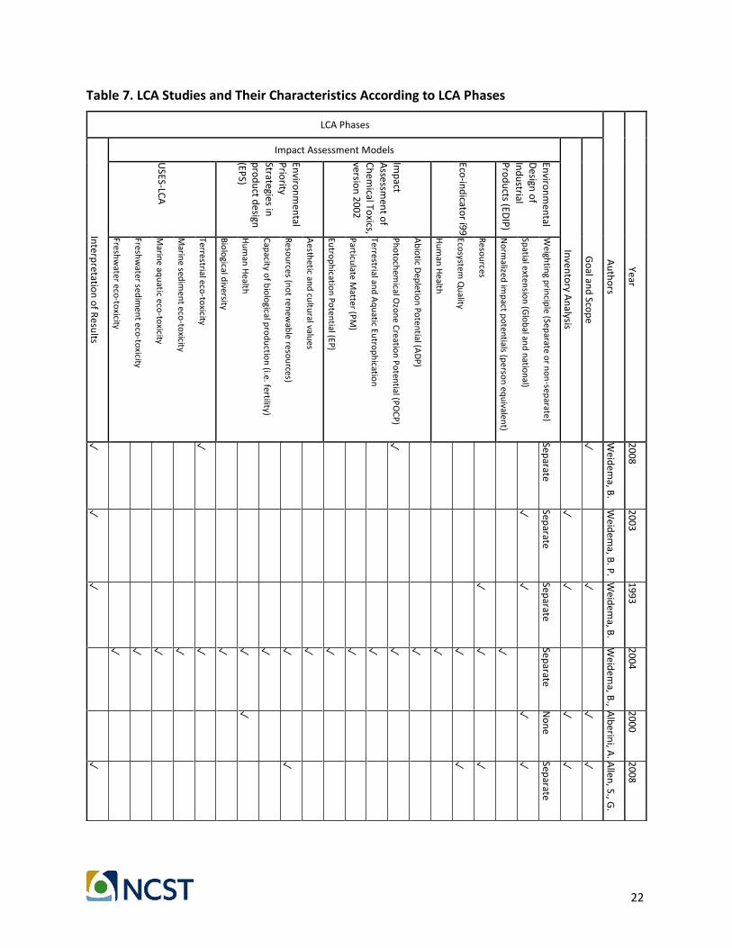
Finally, the researchers develop Table 7, which provides a summary classification of the various references discussed in this section based on the LCA classifications, the phases they consider, and their relationship to risk and uncertainties. Figure 5 provides a visual representation of the identified gaps.

1 Assessment is a process to obtain information through surveying, characterizing, synthesizing, and interpreting primary data sources. 2 Analysis is a process to search for understanding, by taking things apart and studying the parts.

22

Table 7. LCA Studies and Their Characteristics According to LCA Phases

LCA Phases A

uth

ors

Year

Interp

retation

of R

esults

Impact Assessment Models

Inven

tory A

nalysis

Go

al and

Scop

e

USES-LC

A

Enviro

nm

ental

Prio

rity Strategies in

pro

du

ct de

sign

(EP

S)

Imp

act A

ssessmen

t of

Ch

em

ical Toxics,

version

2002

Eco-in

dicato

r i99

Enviro

nm

ental

Design

of

Ind

ustrial

Pro

du

cts (ED

IP)

Freshw

ater eco-to

xicity

Freshw

ater sedim

ent eco

-toxicity

Marin

e aqu

atic eco-to

xicity

Marin

e sedim

ent eco

-toxicity

Terrestrial eco-to

xicity

Bio

logical d

iversity

Hu

man

He

alth

Cap

acity of b

iolo

gical pro

du

ction

(i.e. fertility)

Reso

urces (n

ot ren

ewab

le resou

rces)

Aesth

etic and

cultu

ral values

Eutro

ph

ication

Poten

tial (EP)

Particu

late Matter (P

M)

Terrestrial and

Aq

uatic Eu

trop

hicatio

n

Ph

otoch

emical O

zon

e Creatio

n P

oten

tial (PO

CP

)

Ab

iotic D

epletio

n Po

tential (A

DP

)

Hu

man

He

alth

Ecosystem

Qu

ality

Reso

urces

No

rmalized

imp

act po

tentials (p

erson

equ

ivalent)

Spatial exten

sion

(Glo

bal an

d n

ation

al)

Weigh

ting p

rincip

le (Separate o

r no

n-sep

arate)

✓

✓

✓

Separate

✓

Weid

em

a, B.

P., M

. Thran

e,

P. C

hristen

sen,

J. Schm

idt an

d

S. Løkke

2008

✓

✓

Separate

✓

Weid

em

a, B. P

.

2003

✓

✓

✓

Separate

✓

✓

Weid

em

a, B.

P. (

1993

✓

✓

✓

✓

✓

✓

✓

✓

✓

✓

✓

✓

✓

✓

✓

✓

✓

✓

✓

Separate

Weid

em

a, B.,

T. Ekvall, H.

Peso

nen

, G.

Reb

itzer, G.

Son

ne

man

an

d M

. Sp

ielman

n (2

2004

✓

✓

No

ne

Separate

✓

✓

Alb

erin

i, A.

and

A.

Kru

pn

ick

2000

✓

✓

✓

✓

✓

Separate

✓

✓

Allen

, S., G.

Ham

mo

nd

an

d M

. M

cMan

us (

2008

23

LCA Phases

Au

tho

rs

Year

Interp

retation

of R

esults

Impact Assessment Models

Inven

tory A

nalysis

Go

al and

Scop

e

USES-LC

A

Enviro

nm

ental

Prio

rity Strategies in

pro

du

ct de

sign

(EP

S)

Imp

act A

ssessmen

t of

Ch

em

ical Toxics,

version

2002

Eco-in

dicato

r i99

Enviro

nm

ental

Design

of

Ind

ustrial

Pro

du

cts (ED

IP)

Freshw

ater eco-to

xicity

Freshw

ater sedim

ent eco

-toxicity

Marin

e aqu

atic eco-to

xicity

Marin

e sedim

ent eco

-toxicity

Terrestrial eco-to

xicity

Bio

logical d

iversity

Hu

man

He

alth

Cap

acity of b

iolo

gical pro

du

ction

(i.e. fertility)

Reso

urces (n

ot ren

ewab

le resou

rces)

Aesth

etic and

cultu

ral values

Eutro

ph

ication

Poten

tial (EP)

Particu

late Matter (P

M)

Terrestrial and

Aq

uatic Eu

trop

hicatio

n

Ph

otoch

emical O

zon

e Creatio

n P

oten

tial (PO

CP

)

Ab

iotic D

epletio

n Po

tential (A

DP

)

Hu

man

He

alth

Ecosystem

Qu

ality

Reso

urces

No

rmalized

imp

act po

tentials (p

erson

equ

ivalent)

Spatial exten

sion

(Glo

bal an

d n

ation

al)

Weigh

ting p

rincip

le (Separate o

r no

n-sep

arate)

✓

✓

✓

Separate

✓

✓

Altin

g, L.

1995

✓

✓

✓

✓

No

ne

Separat

e ✓

✓

Bailly,

H. an

d

P.

Brin

cker

ho

ff

1999

No

ne

Separat

e ✓

✓

Bare, J.

2011

✓

✓

✓

✓

✓

✓

Separate

✓

✓

Berglu

nd

, M

. and

P.

Bö

rjesson

2006

✓

✓

✓

✓

✓

✓

Separate

✓

✓

Bu

rnh

am, A

., J. H

an, C

. E. C

lark, M.

Wan

g, J. B.

Du

nn

and

I. P

alou

-Rivera

2011

✓

✓

✓

No

ne

Separat

e ✓

✓

Bu

rritt, R

. L., T. H

ahn

an

d S.

Schalteg

ger

2002

✓

✓

✓

✓

Separate

✓

✓

Ch

en

g, X.

2016

Separate

✓

✓

Ch

eru

bin

i, F. an

d A

. H.

Strøm

man

(

2011

24

LCA Phases

Au

tho

rs

Year

Interp

retation

of R

esults

Impact Assessment Models

Inven

tory A

nalysis

Go

al and

Scop

e

USES-LC

A

Enviro

nm

ental

Prio

rity Strategies in

pro

du

ct de

sign

(EP

S)

Imp

act A

ssessmen

t of

Ch

em

ical Toxics,

version

2002

Eco-in

dicato

r i99

Enviro

nm

ental

Design

of

Ind

ustrial

Pro

du

cts (ED

IP)

Freshw

ater eco-to

xicity

Freshw

ater sedim

ent eco

-toxicity

Marin

e aqu

atic eco-to

xicity

Marin

e sedim

ent eco

-toxicity

Terrestrial eco-to

xicity

Bio

logical d

iversity

Hu

man

He

alth

Cap

acity of b

iolo

gical pro

du

ction

(i.e. fertility)

Reso

urces (n

ot ren

ewab

le resou

rces)

Aesth

etic and

cultu

ral values

Eutro

ph

ication

Poten

tial (EP)

Particu

late Matter (P

M)

Terrestrial and

Aq

uatic Eu

trop

hicatio

n

Ph

otoch

emical O

zon

e Creatio

n P

oten

tial (PO

CP

)

Ab

iotic D

epletio

n Po

tential (A

DP

)

Hu

man

He

alth

Ecosystem

Qu

ality

Reso

urces

No

rmalized

imp

act po

tentials (p

erson

equ

ivalent)

Spatial exten

sion

(Glo

bal an

d n

ation

al)

Weigh

ting p

rincip

le (Separate o

r no

n-sep

arate)

✓

✓

✓

✓

✓

✓

Separate

✓

✓

Ch

ester, M

. an

d A

. H

orvath

2010

✓

✓

✓

✓

✓

✓

✓

No

ne

Separate

✓

✓

Ch

ester, M

. an

d A

. H

orvath

2012

✓

Separate

✓

✓

Fichtn

er, W

., M.

Frank an

d

O. R

entz (

2004

No

ne Sep

arate

Favara, P. J., T.

M. K

rieger, B.

Bo

ugh

ton

, A.

S. Fisher an

d

M. B

hargava

2011

✓

✓

✓

✓

Separate

✓

✓

Finn

veden

, G

., M.

Hau

schild

an

d T.

Ekvall (

2009

✓

No

ne Sep

arate

✓

✓

Finn

veden

, G., M

. Z. H

ausch

ild, T. Ekvall,

J. Gu

iné

e, R.

Heiju

ngs, S.

Hellw

eg, A. K

oeh

ler, D

. Pen

nin

gton

and

S. Su

h (2

0

2009

✓

✓

✓

✓

✓

✓

✓

✓

✓

✓

✓

✓

✓

Separate

✓

Go

edko

op

, M.,

R. H

eijun

gs, M.

Hu

ijbregts, A

. D

e Schryver, J.

Struijs an

d R

. V

an Zelm

(2

2009

25

LCA Phases

Au

tho

rs

Year

Interp

retation

of R

esults

Impact Assessment Models

Inven

tory A

nalysis

Go

al and

Scop

e

USES-LC

A

Enviro

nm

ental

Prio

rity Strategies in

pro

du

ct de

sign

(EP

S)

Imp

act A

ssessmen

t of

Ch

em

ical Toxics,

version

2002

Eco-in

dicato

r i99

Enviro

nm

ental

Design

of

Ind

ustrial

Pro

du

cts (ED

IP)

Freshw

ater eco-to

xicity

Freshw

ater sedim

ent eco

-toxicity

Marin

e aqu

atic eco-to

xicity

Marin

e sedim

ent eco

-toxicity

Terrestrial eco-to

xicity

Bio

logical d

iversity

Hu

man

He

alth

Cap

acity of b

iolo

gical pro

du

ction

(i.e. fertility)

Reso

urces (n

ot ren

ewab

le resou

rces)

Aesth

etic and

cultu

ral values

Eutro

ph

ication

Poten

tial (EP)

Particu

late Matter (P

M)

Terrestrial and

Aq

uatic Eu

trop

hicatio

n

Ph

otoch

emical O

zon

e Creatio

n P

oten

tial (PO

CP

)

Ab

iotic D

epletio

n Po

tential (A

DP

)

Hu

man

He

alth

Ecosystem

Qu

ality

Reso

urces

No

rmalized

imp

act po

tentials (p

erson

equ

ivalent)

Spatial exten

sion

(Glo

bal an

d n

ation

al)

Weigh

ting p

rincip

le (Separate o

r no

n-sep

arate)

✓

✓

✓

✓

No

ne

Separate

✓

✓

Go

edko

op

, M

., P.

Ho

fstetter, R.

Mü

ller-Wen

k

and

R.

Spriem

sma

1998

✓

✓

✓

✓

No

ne

Separate

✓

✓

Go

edko

op

, M

. and

R.

Sprien

sma

2000

✓

✓

✓

Separate

✓

✓

Gu

iné

e, J.

2016

✓

✓

✓

✓

✓

Separate

✓

✓

Gu

iné

e, J. B.

2002

✓

✓

✓

✓

✓

Separate

✓

✓

Gu

ine

e, J. B

., R.

Heiju

ngs, G

. H

up

pe

s, A.

Zamagn

i, P.

Maso

ni, R

. B

uo

nam

ici, T. Ekvall an

d

T. Ryd

berg

(20

2010

✓

✓

✓

✓

Separate

✓

✓

Gu

iné

e, J. B

., G.

Hu

pp

es

and

R.

Heiju

ngs

2001

✓

✓

✓

Separate

✓

✓

Halo

g, A.

and

Y. M

anik (

2016

26

LCA Phases

Au

tho

rs

Year

Interp

retation

of R

esults

Impact Assessment Models

Inven

tory A

nalysis

Go

al and

Scop

e

USES-LC

A

Enviro

nm

ental

Prio

rity Strategies in

pro

du

ct de

sign

(EP

S)

Imp

act A

ssessmen

t of

Ch

em

ical Toxics,

version

2002

Eco-in

dicato

r i99

Enviro

nm

ental

Design

of

Ind

ustrial

Pro

du

cts (ED

IP)

Freshw

ater eco-to

xicity

Freshw

ater sedim

ent eco

-toxicity

Marin

e aqu

atic eco-to

xicity

Marin

e sedim

ent eco

-toxicity

Terrestrial eco-to

xicity

Bio

logical d

iversity

Hu

man

He

alth

Cap

acity of b

iolo

gical pro

du

ction

(i.e. fertility)

Reso

urces (n

ot ren

ewab

le resou

rces)

Aesth

etic and

cultu

ral values

Eutro

ph

ication

Poten

tial (EP)

Particu

late Matter (P

M)

Terrestrial and

Aq

uatic Eu

trop

hicatio

n

Ph

otoch

emical O

zon

e Creatio

n P

oten

tial (PO

CP

)

Ab

iotic D

epletio

n Po

tential (A

DP

)

Hu

man

He

alth

Ecosystem

Qu

ality

Reso

urces

No

rmalized

imp

act po

tentials (p

erson

equ

ivalent)

Spatial exten

sion

(Glo

bal an

d n

ation

al)

Weigh

ting p

rincip

le (Separate o

r no

n-sep

arate)

✓

✓

✓

✓

✓

✓

Separate

✓

✓

Ham

mo

nd

, G

. P., C

. I. Jo

nes an

d Á

. O

'Grad

y

2015

✓

✓

✓

Separate

✓

✓

Hau

schild

, M.

and

J. Po

tting

2005

✓

✓

✓

✓

✓

✓

✓

✓

✓

✓

✓

Separate

✓

✓

Heiju

ngs,

R., J. B

. G

uin

ée, G

. H

up

pe

s, R.

M.

Lankreijer,

H. A

. Ud

o

de

Haes, A

. W

egen

er

Sleesw

ijk, A

. An

sems,

P. Egge

ls, R

. v. Du

in

and

H. D

e G

oed

e

1992

✓

✓

✓

✓

✓

✓

✓

✓

✓

✓

✓

✓

✓

✓

Separate

✓

✓

Cu

rran, M

. A.

2013

Separate

✓

✓

Cu

rran, M

. A.

1993

✓

✓

✓

Separate

✓

✓

Co

nso

li, F., S. o

. E. To

xicolo

gy an

d

Ch

em

istry

1993

✓

✓

✓

✓

✓

✓

✓

✓

✓

✓

✓

Separate

✓

✓

Co

bas, E., C

. H

end

rickson

, L. Lave an

d F.

McM

ichael

1995

27

LCA Phases

Au

tho

rs

Year

Interp

retation

of R

esults

Impact Assessment Models

Inven

tory A

nalysis

Go

al and

Scop

e

USES-LC

A

Enviro

nm

ental

Prio

rity Strategies in

pro

du

ct de

sign

(EP

S)

Imp

act A

ssessmen

t of

Ch

em

ical Toxics,

version

2002

Eco-in

dicato

r i99

Enviro

nm

ental

Design

of

Ind

ustrial

Pro

du

cts (ED

IP)

Freshw

ater eco-to

xicity

Freshw

ater sedim

ent eco

-toxicity

Marin

e aqu

atic eco-to

xicity

Marin

e sedim

ent eco

-toxicity

Terrestrial eco-to

xicity

Bio

logical d

iversity

Hu

man

He

alth

Cap

acity of b

iolo

gical pro

du

ction

(i.e. fertility)

Reso

urces (n

ot ren

ewab

le resou

rces)

Aesth

etic and

cultu

ral values

Eutro

ph

ication

Poten

tial (EP)

Particu

late Matter (P

M)

Terrestrial and

Aq

uatic Eu

trop

hicatio

n

Ph

otoch

emical O

zon

e Creatio

n P

oten

tial (PO

CP

)

Ab

iotic D

epletio

n Po

tential (A

DP

)

Hu

man

He

alth

Ecosystem

Qu

ality

Reso

urces

No

rmalized

imp

act po

tentials (p

erson

equ

ivalent)

Spatial exten

sion

(Glo

bal an

d n

ation

al)

Weigh

ting p

rincip

le (Separate o

r no

n-sep

arate)

✓

✓

✓

✓

✓

✓

✓

✓

Separate

✓

✓

Ch

ristiansen

, K

., L. Ho

ffman

, Y. V

irtane

n, V

. Ju

ntilla, A

.

Rø

nn

ing, T.

Ekvall and

G.

Finn

veden

1995

✓

✓

✓

✓

✓

✓

✓

Separate

✓

✓

Mo

riguch

i, Y., Y. K

on

do

an

d H

. Sh

imizu

1993

✓

✓

✓

✓

✓

✓

✓

✓

Separate

✓

✓

Nah

lik, M. J.,

A. T. K

aehr,

M. V

. C

he

ster, A.

Ho

rvath an

d

M. N

. Tap

tich

2016

✓

✓

✓

✓

✓

✓

✓

✓

Separate

✓

✓

Sand

én, B

. A.

and

M.

Karlströ

m

2007

✓

✓

✓

✓

✓

Separate

✓

✓

Reb

itzer, G., T.

Ekvall, R.

Frischkn

ech

t, D

. Hu

nkeler, G

.

No

rris, T. R

ydb

erg, W.-P

. Sch

mid

t, S. Su

h, B

. P.

Weid

em

a and

D. W

. P

enn

ingto

n

2004

✓

✓

✓

✓

✓

✓

✓

Separate

✓

✓

Vald

ivia, S., C.

M. U

gaya, J. H

ilde

nb

rand

, M

. Traverso, B

.

Mazijn

and

G.

Son

ne

man

n

2013

✓

✓

✓

✓

✓

✓

✓

✓

✓

Separate

✓

✓

Tukker, A

., G.

Hu

pp

es, J.

Gu

iné

e, R.

Heiju

ngs, A

.

de

Ko

nin

g, L. van

Oers, S.

Suh

, T. G

eerken

, M.

Van

Ho

lde

rbe

ke an

d B

. Jansen

2006

28

LCA Phases

Au

tho

rs

Year

Interp

retation

of R

esults

Impact Assessment Models

Inven

tory A

nalysis

Go

al and

Scop

e

USES-LC

A

Enviro

nm

ental

Prio

rity Strategies in

pro

du

ct de

sign

(EP

S)

Imp

act A

ssessmen

t of

Ch

em

ical Toxics,

version

2002

Eco-in

dicato

r i99

Enviro

nm

ental

Design

of

Ind

ustrial

Pro

du

cts (ED

IP)

Freshw

ater eco-to

xicity

Freshw

ater sedim

ent eco

-toxicity

Marin

e aqu

atic eco-to

xicity

Marin

e sedim

ent eco

-toxicity

Terrestrial eco-to

xicity

Bio

logical d

iversity

Hu

man

He

alth

Cap

acity of b

iolo

gical pro

du

ction

(i.e. fertility)

Reso

urces (n

ot ren

ewab

le resou

rces)

Aesth

etic and

cultu

ral values

Eutro

ph

ication

Poten

tial (EP)

Particu

late Matter (P

M)

Terrestrial and

Aq

uatic Eu

trop

hicatio

n

Ph

otoch

emical O

zon

e Creatio

n P

oten

tial (PO

CP

)

Ab

iotic D

epletio

n Po

tential (A

DP

)

Hu

man

He

alth

Ecosystem

Qu

ality

Reso

urces

No

rmalized

imp

act po

tentials (p

erson

equ

ivalent)

Spatial exten

sion

(Glo

bal an

d n

ation

al)

Weigh

ting p

rincip

le (Separate o

r no

n-sep

arate)

✓

✓

✓

✓

✓

✓

✓

✓

✓

✓

Separate

✓

✓

Toffo

letto, L.,

C. B

ulle, J.

Go

din

, C. R

eid

and

L.

Desch

ên

es

2007

Separate

✓

Tillman

, A.-

M., T. Ekvall,

H. B

aum

ann

an

d T.

Ryd

berg

1994

✓

✓

✓

✓

✓

✓

No

ne

Separate

✓

✓

Tillman

, A

.-M.

2000

✓

✓

✓

Separate

✓

✓

Tho

ft-C

hristen

sen,

P.

2012

✓

✓

✓

✓

✓

✓

✓

Separate

✓

✓

Swart, P

., R.

A. A

lvarenga

and

J. Dew

ulf

2015

✓

✓

✓

✓

✓

✓

✓

No

ne

Separat

e ✓

✓

Steen,

B.

2005

✓

✓

✓

Separate

✓

✓

Steen, B

.

1999

29

LCA Phases

Au

tho

rs

Year

Interp

retation

of R

esults

Impact Assessment Models

Inven

tory A

nalysis

Go

al and

Scop

e

USES-LC

A

Enviro

nm

ental

Prio

rity Strategies in

pro

du

ct de

sign

(EP

S)

Imp

act A

ssessmen

t of

Ch

em

ical Toxics,

version

2002

Eco-in

dicato

r i99

Enviro

nm

ental

Design

of

Ind

ustrial

Pro

du

cts (ED

IP)

Freshw

ater eco-to

xicity

Freshw

ater sedim

ent eco

-toxicity

Marin

e aqu

atic eco-to

xicity

Marin

e sedim

ent eco

-toxicity

Terrestrial eco-to

xicity

Bio

logical d

iversity

Hu

man

He

alth

Cap

acity of b

iolo

gical pro

du

ction

(i.e. fertility)

Reso

urces (n

ot ren

ewab

le resou

rces)

Aesth

etic and

cultu

ral values

Eutro

ph

ication

Poten

tial (EP)

Particu

late Matter (P

M)

Terrestrial and

Aq

uatic Eu

trop

hicatio

n

Ph

otoch

emical O

zon

e Creatio

n P

oten

tial (PO

CP

)

Ab

iotic D

epletio

n Po

tential (A

DP

)

Hu

man

He

alth

Ecosystem

Qu

ality

Reso

urces

No

rmalized

imp

act po

tentials (p

erson

equ

ivalent)

Spatial exten

sion

(Glo

bal an

d n

ation

al)

Weigh

ting p

rincip

le (Separate o

r no

n-sep

arate)

✓

✓

Separate

✓

✓

Seurin

g, S.

2004

✓

✓

✓

No

ne Sep

arate

✓

✓

Searchin

ger, T., R.

Heim

lich, R

. A.

Ho

ugh

ton

, F. Do

ng,

A. Elo

beid

, J.

Fabio

sa, S. Tokgo

z, D

. Hayes an

d T.-H

. Yu

2008

✓

✓

✓

✓

✓

✓

✓

No

ne

✓

✓

Schm

idt, J.

H., P

. H

olm

, A.

Merrild

and

P.

Ch

ristense

n

2007

30

Figure 5. LCA Studies Classifications According to Phases

0

20

40

60

80

100

120

Classification of Studies (%)

Goal and Scope

Inventory Analysis

Impact Assessment Models Environmental Design of Industrial Products (EDIP) Normalized impact potentials (person equivalent)

Impact Assessment Models Environmental Design of Industrial Products (EDIP) Spatial extension (Global and national)

Impact Assessment Models Environmental Design of Industrial Products (EDIP) Weighting principle (Separate or non-separate)

Impact Assessment Models Eco-indicator i99 Human Health

Impact Assessment Models Eco-indicator i99 Ecosystem Quality

Impact Assessment Models Eco-indicator i99 Resources

Impact Assessment Models Environmental Priority Strategies in product design (EPS) Biological diversity

Impact Assessment Models Environmental Priority Strategies in product design (EPS) Human Health

Impact Assessment Models Environmental Priority Strategies in product design (EPS) Capacity of biological production

Impact Assessment Models Environmental Priority Strategies in product design (EPS) Resources (not renewable resources)

Impact Assessment Models Environmental Priority Strategies in product design (EPS) Aesthetic and cultural values

Impact Assessment Models Impact Assessment of Chemical Toxics, version 2002 Eutrophication Potential (EP)

Impact Assessment Models Impact Assessment of Chemical Toxics, version 2002 Particulate Matter (PM)

Impact Assessment Models Impact Assessment of Chemical Toxics, version 2002 Terrestrial and Aquatic Eutrophication

Impact Assessment Models Impact Assessment of Chemical Toxics, version 2002 Photochemical Ozone Creation Potential (POCP)

Impact Assessment Models Impact Assessment of Chemical Toxics, version 2002 Abiotic Depletion Potential (ADP)

Impact Assessment Models USES-LCA Freshwater eco-toxicity

Impact Assessment Models USES-LCA Freshwater sediment eco-toxicity

Impact Assessment Models USES-LCA Marine aquatic eco-toxicity

Impact Assessment Models USES-LCA Marine sediment eco-toxicity

Impact Assessment Models USES-LCA Terrestrial eco-toxicity

Interpretation of Results

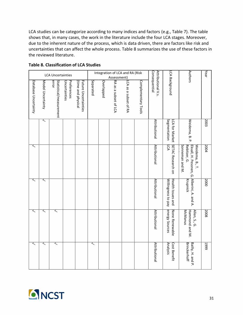
31

LCA studies can be categorize according to many indices and factors (e.g., Table 7). The table shows that, in many cases, the work in the literature include the four LCA stages. Moreover, due to the inherent nature of the process, which is data driven, there are factors like risk and uncertainties that can affect the whole process. Table 8 summarizes the use of these factors in the reviewed literature.

Table 8. Classification of LCA Studies

LCA Uncertainties Integration of LCA and RA (Risk

Assessment)

Attrib

utio

nal V

.s.

Co

nseq

uen

tial

LCA

Backgro

un

d

Au

tho

rs

Year

Datab

ase Un

certainty

Mo

del U

ncertain

ty

Statistical/measu

remen

t

error

Preferen

ces

Un

certainties

Futu

re Un

certainties

(time an

d ph

ysical system

)

Separated

Overlap

pe

d

RA

as a sub

set of LCA

LCA

as a sub

set of R

A

Co

mp

lemen

tary Too

ls

✓

Attrib

utio

nal

LCA

for M

arket

Segmen

tation

Weid

ema, B

. P.

2003

✓

Attrib

utio

nal

SETAC

Research

on

LCA

Weid

ema, B

., T.

Ekvall, H. P

eson

en, G

. R

ebitzer, G

.

Son

ne

man

and

M.

Spielm

ann

2004

✓

✓

Attrib

utio

nal

Health

Issues an

d

Willin

gness to p

ay

Alb

erini, A

. and

A.

Kru

pn

ick

2000

✓

✓

✓

Attrib

utio

nal

No

ne R

enew

able

energy So

urces

Allen

, S., G.

Ham

mo

nd

and

M.

McM

anu

s

2008

✓

✓

✓

✓

Attrib

utio

nal

Co

st Ben

efit

An

alysis

Bailly, H

. and

P.

Brin

ckerho

ff

1999

32

LCA Uncertainties Integration of LCA and RA (Risk

Assessment)

Attrib

utio

nal V

.s.

Co

nseq

uen

tial

LCA

Backgro

un

d

Au

tho

rs

Year

Datab

ase Un

certainty

Mo

del U

ncertain

ty

Statistical/measu

remen

t

error

Preferen

ces

Un

certainties

Futu

re Un

certainties

(time an

d ph

ysical system

)

Separated

Overlap

pe

d

RA

as a sub

set of LC

A

LCA

as a sub

set of R

A

Co

mp

lemen

tary Too

ls

✓

✓

✓

✓

✓

Co

nseq

uen

tial

Fuzzy Lo

gic in LC

A

Ch

eng, X.

2016

✓

Attrib

utio

nal

Clean

er Energy

Pro

du

ction

Fichtn

er, W., M

.

Frank an

d O

. R

entz

2004

✓

✓

✓

Attrib

utio

nal

LCA

develo

pm

ent

Finn

veden

, G., M

. Z.

Hau

schild

, T. Ekvall, J. G

uin

ée, R. H

eijun

gs, S.

Hellw

eg, A. K

oeh

ler, D.

Pen

nin

gton an

d S. Su

h

(20

2009

✓

No

ne

Imp

act assessmen

t

Meth

od

olo

gy

Go

edko

op

, M., P

.

Ho

fstetter, R. M

üller-W

enk an

d R

. Spriem

sma

1998

✓

Attrib

utio

nal

LCSA

Gu

inée, J.

2016

✓

✓

✓

Attrib

utio

nal

EDIP

develo

pm

ent

Hau

schild

, M. an

d

J. Po

tting

2005

33

LCA Uncertainties Integration of LCA and RA (Risk

Assessment)

Attrib

utio

nal V

.s.

Co

nseq

uen

tial

LCA

Backgro

un

d

Au

tho

rs

Year

Datab

ase Un

certainty

Mo

del U

ncertain

ty

Statistical/measu

remen

t

error

Preferen

ces

Un

certainties

Futu

re Un

certainties

(time an

d ph

ysical system

)

Separated

Overlap

pe

d

RA

as a sub

set of LC

A

LCA

as a sub

set of R

A

Co

mp

lemen

tary Too

ls

✓

✓

Attrib

utio

nal

LCA

develo

pm

ent

Heiju

ngs, R

., J. B. G

uin

ée,

G. H

up

pes, R

. M.

Lankreijer, H

. A. U

do

de

Haes, A

. Wege

ner

Sleesw

ijk, A. A

nsem

s, P.

Eggels, R. v. D

uin

and

H.

De G

oed

e

1992

✓

✓

✓

Attrib

utio

nal

LCA

in

Transp

ortatio

n

Nah

lik, M. J., A

.

T. Kaeh

r, M. V

. C

hester, A

.

Ho

rvath an

d M

. N

. Taptich

2016

✓

✓

✓

✓

Co

nseq

uen

tial

Co

nseq

uen

tial

LCA

Sand

én

, B. A

. and

M. K

arlström

2007

✓

Attrib

utio

nal

EIPRO

Tukker, A

., G.

Hu

pp

es, J. G

uin

ée, R.

Heiju

ngs, A

. de

Ko

nin

g, L. van

Oers, S. Su

h, T.

Gee

rken, M

. Van

H

old

erbeke an

d

B. Jan

sen

2006

✓

✓

✓

✓

Attrib

utio

nal

Can

adian

LCA

(LUC

AS)

Toffo

letto, L., C.

Bu

lle, J. Go

din, C

. R

eid an

d L.

Desch

êne

s

2007

✓

✓

Attrib

utio

nal

LCA

develo

pm

ent

Tillman

, A.-M

., T.

Ekvall, H.

Bau

man

n an

d T.

Ryd

be

rg

1994

✓

✓

✓

Attrib

utio

nal

LCA

Extensio

ns

Tillman

, A.-M

.

2000

34

LCA Uncertainties Integration of LCA and RA (Risk

Assessment)

Attrib

utio

nal V

.s.

Co

nseq

uen

tial

LCA

Backgro

un

d

Au

tho

rs

Year

Datab

ase Un

certainty

Mo

del U

ncertain

ty

Statistical/measu

remen

t

error

Preferen

ces

Un

certainties

Futu

re Un

certainties

(time an

d ph

ysical system

)

Separated

Overlap

pe

d

RA

as a sub

set of LC

A

LCA

as a sub

set of R

A

Co

mp

lemen

tary Too

ls

✓

Attrib

utio

nal

LCA

develo

pm

ent

Swart, P

., R. A

.

Alvaren

ga and

J. D

ewu

lf

2015

✓

✓

✓

Attrib

utio

nal

LCA

Extensio

ns

Steen

, B.

1999

✓

Attrib

utio

nal

LCSA

Seurin

g, S.

2016

✓

Attrib

utio

nal

LCSA

Searchin

ger, T.,

R. H

eimlich, R

. A.

Ho

ugh

ton

, F.

Do

ng, A

. Elob

eid,

J. Fabio

sa, S.

Tokgo

z, D. H

ayes

and

T.-H. Yu

2008

✓

Attrib

utio

nal

LCA

develo

pm

ent

Schm

idt, J. H

., P.

Ho

lm, A

. Merrild

an

d P

.

Ch

ristensen

2007

35

Figure 6. LCA Studies Classifications According to Uncertainties and Risk Factors

0

5

10

15

20

25

Dat

abas

e U

nce

rtai

nty

Mo

del

Un

cert

ain

ty

Stat

isti

cal/

mea

sure

men

t er

ror

Pre

fere

nce

s U

nce

rtai

nti

es

Futu

re U

nce

rtai

nti

es (

tim

e an

dp

hys

ical

sys

tem

)

Sep

ara

ted

Ove

rlap

ped

RA

as

a su

bse

t o

f LC

A

LCA

as

a su

bse

t o

f R

A

Co

mp

lem

enta

ry T

oo

ls

LCA Uncertainties Integration of LCA and RA (Risk Assessment)

36

V. Impact Assessment Methodologies

Relevant to this report is the third phase of an LCA that refers to the assessment of impacts of the specific product or service (according to certain endpoints and midpoints). These impacts can be in the form of eco system quality, human health, and natural resources, among others. This phase evaluates all or some parts of these characterization factors (CFs) through defined and specific methodologies, and use weighting factors to aggregate life cycle impacts. The level of uncertainty and the coverage of impact categories are different depending on whether they are assessing mid-point or end-point indicators and contributes to different impact scores. Usually, equivalency factors express midpoint, while end-point indicators refer to the main factors of human health, ecosystem health, and resource availability. Social and Environmental Impact Assessment Methodologies are among the most common methods. The international standard ISO14001:2004 defines an impact as “…any change to the environment, whether adverse or beneficial, wholly or partially resulting from an organization’s environmental aspects…” The ISO also define environmental aspect as the “…element of an organization’s activities or products or services that can interact with the environment…” (Whitelaw, 2004; Finkbeiner et al., 2006).

Environmental Impact Assessment (EIA) Methodologies

EIA methodologies represent a wide variety of methods to trace back the environmental effects of a product or service. Considering the multitude of methods, the specific requirements of the study will help determine the most appropriate assessment to use. The most commonly used methodologies include the methods outlined below.

Ad hoc methods

These methods consider a qualitative index to assess environmental impacts, usually assessed by team of experts. The results are informed using simple terms without much detail on the specific parameter changes due to impacts. One of the major limitations is that these methods may not consider all the relevant impact factors, and there is a lack of normalization between different groups causing inconsistency in the analysis (Lohani et al., 1997).

Matrix methods

Matrix methods are among the popular methods for impact assessment due to their user-friendly representation of factors. The rationale for these methods is to identify the relationships and interactions between the processes (project actions) and the environmental impact factors. Early on, these methods compared in one axis, the list of project activities, and the environmental components on the other. The matrices provided a simple representation of the cause and effect relationship with either qualitative or quantitative values. However, these methods provide limited applicability to identify indirect impacts (Lohani et al., 1997).

37

Networks-based Methods

Matrix methods can also be categorized in many ways, one of which are network models, which incorporate long-term impacts of the project activity. One of the improvements from static matrix methods is the use of network-based conceptual models to represent the pathways or causal chains for the relationships between cause and effect. Several categories classify the impacts, e.g., primary, secondary or tertiary. The major strength of the network approach is its ability to indicate both direct and indirect environmental impacts. Specifically, there are many methodologies to implement LCIA studies; Annex B summarizes these methodologies. Recently, Wolf et al. (2012) assessed the various EIA methodologies based on the included impact factors (see Error! Reference source not found.). In the table, “O” indicates if a specific impact is just considered in the methodology but not furthered investigated; “M” indicates that a midpoint value is available and furthered investigated; and, “E” refers to the availability of an endpoint value that is furthered investigated.

38

Table 9. Characterization Models for Impact Assessment

Clim

ate

chan

ge

Ozo

ne

dep

leti

on

Res

pir

ato

ry

ino

rgan

ics

Hu

man

to

xici

ty

Ion

izin

g ra

dia

tio

n

Eco

to

xici

ty

Ozo

ne

fo

rmat

ion

Aci

dif

icat

ion

Ters

est.

Eu

tro

ph

icat

ion

Aq

uat

ic

Eutr

op

hic

atio

n.

Res

ou

rce

C

on

sum

pti

on

Oth

ers

Res

ou

rce

C

on

sum

pti

on

Oth

ers

Oth

ers

CML 2002 (Guinée, 2002)

O O M O O M M M M O M

ECO-indicator 99 (Goedkoop and Spriensma, 2000)

E E E O O E E E E E

EDIP 2003/EDIP97 (Hauschild and Potting, 2005)

O M O M O M M M M M M

Wo

rk

Envi

ron

men

t R

oad

no

ise

EPS 2000 (Steen, 1999)

E E E E O E E O O O E E

IMPACT 2002+ (Jolliet and Fantke, 2015)

O O E M E

O M E

E M E

O M E

E

LIME (Itsubo et al., 2012)

E E M E O M E O E E E Indoor air

LUCAS (Toffoletto et al., 2007)

O o o o o o o o o O

MEEuP (Kemna et al., 2005)

O O M M M M M M M Water

ReCiPe (Goedkoop et al., 2009)

M E E M E

M E

O M E

M E

M E

O M E M E

E

Swiss Ecosacrcity 07 (Swart et al., 2015)

O O O O M E M O O O O M E

Water

End

ocr

ine

d

isru

pto

rs

TRACI (Bare, 2011)

O O M M M M M O M O

Specific methods to be evaluated

Eco

logi

cal

Foo

t P

rin

t

USE

Tox

USE

Tox

Eco

logi

cal

foo

tpri

nt

Specific methods of potential interest (not to be evaluated)

Wat

son

(B

ach

man

n)

Eco

to

xici

ty o

f ra

dia

tio

n

(Lap

lace

et

al.)

Eco

Sen

se

Eco

Sen

se

Mei

jer

ind

oo

r ai

r U

NEP

In

do

or

air

Source: (Wolf et al., 2012)

39

Economic Cost-Benefit Analysis (CBA)

Cost-benefit analyses (CBA) are one of the common approaches to quantitatively asses the benefits of a project. This traditional approach evaluates economic factors such as welfare, resources, and public finance. Table 10 provides an overview of the typical steps to conduct a cost-benefit analysis and the types of questions it addresses. Table 10. Cost and Benefit Analysis

Steps Questions? Criteria

Preliminary Considerations

Problem statement

Which costs and benefits to consider?

How to value them?

What is the interest rate to discount them?

Investigating the General Issue

Main Questions

Enumeration of Costs and benefits (Examples)

Project definitions

Externalities Secondary benefits

Project Life time

Costs and benefit evaluation

Relevant Prices

Non-marginal Changes Market Imperfections

Taxes and Controls

Unemployment Ratio Collective Goods

Intangibles

Interest Rate

Time preference rate

Opportunity cost rate Adjustment for uncertainties

Interest Rate Calculations

Principles, and practice

Relevant Consideration

Distributional Constraints

Budgetary Constraints

Supply Chain Constraints

Final Considerations

Investment criteria Policy vs. Decision making Consideration

Source: (Prest and Turvey, 1965)

In general, a project is economically feasible and justifiable to do when the benefits outweigh its costs. An ideal cost benefit analysis evaluates all the aspects of the project including its desirability, social preferences, and the target policy. Logically, preferred projects are the ones with the highest net benefits compared to their net costs. The methods use a discount rate to estimate the value of future costs and benefits (Alberini and Krupnick, 2000).

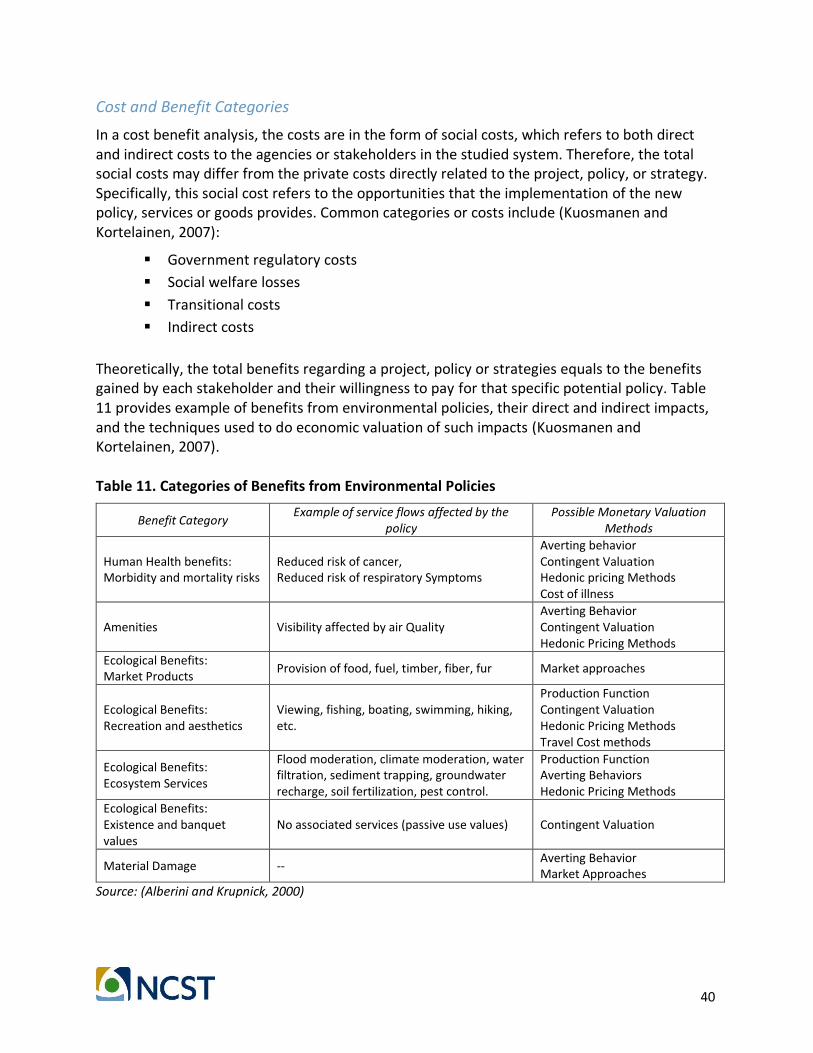
40

Cost and Benefit Categories

In a cost benefit analysis, the costs are in the form of social costs, which refers to both direct and indirect costs to the agencies or stakeholders in the studied system. Therefore, the total social costs may differ from the private costs directly related to the project, policy, or strategy. Specifically, this social cost refers to the opportunities that the implementation of the new policy, services or goods provides. Common categories or costs include (Kuosmanen and Kortelainen, 2007):

▪ Government regulatory costs

▪ Social welfare losses

▪ Transitional costs

▪ Indirect costs

Theoretically, the total benefits regarding a project, policy or strategies equals to the benefits gained by each stakeholder and their willingness to pay for that specific potential policy. Table 11 provides example of benefits from environmental policies, their direct and indirect impacts, and the techniques used to do economic valuation of such impacts (Kuosmanen and Kortelainen, 2007). Table 11. Categories of Benefits from Environmental Policies

Benefit Category Example of service flows affected by the

policy Possible Monetary Valuation

Methods

Human Health benefits: Morbidity and mortality risks

Reduced risk of cancer, Reduced risk of respiratory Symptoms

Averting behavior Contingent Valuation Hedonic pricing Methods Cost of illness

Amenities Visibility affected by air Quality Averting Behavior Contingent Valuation Hedonic Pricing Methods

Ecological Benefits: Market Products

Provision of food, fuel, timber, fiber, fur Market approaches

Ecological Benefits: Recreation and aesthetics

Viewing, fishing, boating, swimming, hiking, etc.

Production Function Contingent Valuation Hedonic Pricing Methods Travel Cost methods

Ecological Benefits: Ecosystem Services

Flood moderation, climate moderation, water filtration, sediment trapping, groundwater recharge, soil fertilization, pest control.

Production Function Averting Behaviors Hedonic Pricing Methods

Ecological Benefits: Existence and banquet values

No associated services (passive use values) Contingent Valuation

Material Damage -- Averting Behavior Market Approaches

Source: (Alberini and Krupnick, 2000)

41

Environmental Cost-Benefit Analysis

CBA and LCA are decision-making tools regarding the impacts of projects, products and procedures; however, they may have different scopes and objectives. While CBA may consider a wide range of impacts, LCA mostly focuses on environmental and health impacts. Similarly, there are distinctions between Life Cycle Costing (LCC) and LCA (Finkbeiner et al., 2006; Lippiatt, 2017). LCC evaluates products, and procedures based on their monetary values, while LCA focusses on the environmental consequences resulting from a product. These distinctions contrast their degree and strategy of application (Lippiatt, 2017). LCC usually concentrates on the use phase, and could be considered a sub-category of a full LCA (Lippiatt, 2017). For instance, there are cases in which a LCC and a LCA differ in their consideration of the physical flows, processes, cash flows and their timing, as well as the risk of the costs. Despite the differences, there are models aiming at properly bonding LCA and LCC.

PTLaser

This method builds on the LCA stages and adds monetary values, measurements of time, and allocates capacities to the physical flow to properly account for the costs in the LCC (Norris, 2001). The major contribution of this model is the use of vulnerability and hazards concepts. This method builds on a chance-constrained framework to evaluate scenarios that can happen with some probabilities. (Norris, 2001).

TCAce

TCAce is another framework to integrate LCC and LCA with a decision making environment (Norris, 2001). Contrary to PTLaser, this method uses the outcome of a LCA and estimates the costs using conventional monetary examinations and considers the inconsequential costs (Norris, 2001).

LCA and Cost-Benefit Applications in Transportation

Transportation applications have used LCA and cost-benefit analyses to identify the most sustainable transportation mode, vehicle, or fuel pathway. Similar to the previous descriptions, LCA can evaluate the impacts of transportation processes from raw material extraction, and all the subsequent processes through its life cycle. Different stakeholders can use the methods for decision-making. Although general cost-benefits methods can evaluate a wide range of impacts, indirect environmental costs are sometimes ignored or could be the main focus of the method’s implementation (Manzo and Salling, 2016). However, the traditional cost-benefit methods have not fully considered the ecological sustainability and the impact of the transportation systems on this aspect (Manzo and Salling 2016). Chester et al. (2010) valuated passenger transportation systems including car, buses, trains and airplanes and their relative LCA. The study concluded that, inputs from life-cycle energy and GHG emissions will increase the operating costs from 31% (air) to 155% (rail). They also evaluated the energy consumption in transportation in three metropolitan regions and concluded that considering the environmental impact factors, the energy consumption and emissions increase up to 20 times.

42

In addition to the energy consumption and emissions, some of the studies incorporate the land use dimension. For instance, Kimball et al. (2013) show that the environmental impacts of the infrastructure construction, vehicle industries and energy consumption associated with public transportation are considerable.

Regarding the High-speed rail corridor in California, Chester and Horvath (2010) proposed an LCA analysis that showed high-speed rail transportation system in California may change travel behavior and travel demand in a way that results in environmental emissions reduction, while this system may also change the traffic dynamic and result in increased environmental emissions. Thoft-Christensen (2012) used LCA to analyze a motorway infrastructure investment and concluded that building the new infrastructure would impose higher expenses than the maintenance costs of the existing infrastructure. Chester and Horvath (2012) also evaluated the modal transfer from private vehicles to public transit modes. In this study, the authors believe that new technologies may help reduce environmental footprints, while results indicate that the lifecycle regarding the vehicle, infrastructure, and energy production may increase environmental emissions. There are just a handful of studies combining LCA and Cost-Benefit Analysis (CBA) in transportation. These existing studies highlight the importance of evaluating the environmental impacts of transportation infrastructure and operations. Salling and Leleur (2015) developed a tool to analyze the transport infrastructure projects through CBA by incorporating a LCA module into the UNITE-DSS model (see Figure 7). The proposed UNITE-DSS model consists of two parts: deterministic and stochastic. The deterministic component deals with common socio-economic indicators using CBA approaches evaluating the Net Present Value (NPV), Benefit Cost Ratio (BCR), and the Internal Rate of Return (IRR). The stochastic component considers the uncertainty analysis of construction costs, in addition to the transport demand forecast, mostly based on Monte-Carlo Simulation (MCS).

43

Figure 7. UNITE-DSS Model Framework (Halog and Manik, 2016)

Nahlik et al. (2015) proposed a LCA framework for freight transportation systems focusing on the flows originating from or destined to California. The freight transportation mode is limited to rail, Ocean Going Vessels (OGV), and road transportation, which divided into to medium heavy-duty vehicles (MHD), and Heavy-Heavy Duty vehicles (HHD). The study considers energy inputs and air emissions categorized as GHG, CO, non-methane volatile organic compounds (NMVOC), NOX, SO2, PM10, and PM2.5. The study transferred the individual emission categories into carbon dioxide equivalent (CO2eq) for ease of calculations. The study uses a number of databases to estimate the environmental impacts of the transport of goods using the various modes and the established boundaries. The LCA stages include vehicle operation/propulsion, vehicle manufacturing and maintenance, infrastructure, and energy production. The estimates use EMFAC and CARB data for assessing vehicle operations, CA-GREET for energy production and mix grids, PaLATE for infrastructure emissions, and SimaPro and Ecoinvent to calculate the emissions regarding vehicle manufacturing and maintenance. The study considers different scenarios to assess the movement of goods intrastate and the imports and exports. For intrastate transportation, the analyses consider rail and over the road transport, and consider combinations of modes (railway and use of trucks), and using (MHD and HHDO) trucks for intrastate transportation. The importing and exporting goods to/from the state is also considered through the rail, rail and trucks (MHD, HHD), trucks and the combination of trucks and ships) for imports and exports. Limiting to the transportation component, the study finds that truck movements (vehicle operations) contribute the largest amount of emissions. Moreover, the study concludes that ocean going ships are among the modes of transportation that have the lowest emissions (Nahlik et al., 2015). This study provides a general framework to estimate the environmental impacts of the entire transportation sector, whether in or outside California. Figure 8 provides an overview of the LCA results in the state (Nahlik et al., 2015).

44

Figure 8. California Intrastate LCA results (Nahlik et al., 2015)

California Life-Cycle Benefit/Cost Analysis Model (Cal-B/C)

One special method that combines LCA and CBA is the California Life-Cycle Benefit/Cost Analysis Model (CAL-B/C). This method provides a practical approach for economic evaluations regarding highways, and transit systems in the State of California (Bailly and Brinckerhoff, 1999). The California Department of Transportation (Caltrans) developed the Cal-B/C as a CBA for highway projects as a spreadsheet model. The model provides analyses based on annual transit ratios and average daily traffic in a highway. The benefits of the model are considered to be in four categories of time savings, reducing vehicle operation costs, and emissions reductions (CO, NOx, PM10, VOC). Cost categories consider annual operating costs and life cycle investment costs. Furthermore, the model incorporates different transportation modes including passenger, rail, light rail, and bus. The method estimates the impacts over the life of the project in the form of life cycle costs/benefits, cost-benefit ratio, projects pay back ratio, the investment return rate, and net present values (Langdon, 2006). Typically, the factors that affect the cost of travel are wage rates, trip purposes, and the amount of time saved or lost. Regarding the value of time, this method incorporates different analyses dependent on mode, route, speed, and dwelling choices. The cost estimates also include congestion, the level of service, and waiting/walking time to destination (Bailly and Brinckerhoff, 1999). The model has capabilities to estimate the cost considering different vehicle types, driver behaviors, and passengers. The model builds on the HERS, StratBENCOST, and STEAM models. Although there are many complexities regarding the evaluation of the cost-benefits in transportation models, models like StratBENCOST and STEAM, account for some environmental costs (Bailly and Brinckerhoff, 1999). On the other hand, the STEAM model estimates the environmental costs more holistically and takes external effects like global warming and noise into account. STEAM calculates the emissions more precisely by using changes in VMT and number of vehicle trips (Bailly and Brinckerhoff, 1999). Figure 9 displays an example flow of using the CAL-B/Co to estimate effects of a highway project on air pollution.

45

Figure 9. Dollar Value on the Air-pollution Effects of a Highway Project (Bailly and Brinckerhoff, 1999)

Summary

LCA provides a general system to recognize and assess the impacts of systems, products, and processes (Matthews et al., 2002). There has been an evolution of both LCA and CBA frameworks, and their combination have led to frameworks that could fully assess the various impacts. However, there are contrasting views and objectives for the selection and implementation of an assessment methodology. For example, Table 12 shows the differences between LCA and some supply chain management perspectives. Table 12. Modeling Approaches for Life Cycle Assessment and Supply Chain Management

Life Cycle Perspective Supply chain Management Perspective

Objective of Study Sustainability measurement in support of a decision

Supporting implementation of a decision or decision rule

Dependent Variable Environmental impacts per functional unit

Performance (cost, profit, or other) per unit time

Scope of considered system

Broader system boundary including different life cycle stages

Often limited to the stages that are immediately related to the decision

Environmental Impacts Considered

Usually multidimensional Often Single-Dimensional

Impact of Production Function

Linear in Volume Nonlinear, Complex

Economic Structure od model

Usually single-agent Multiple agents; incentives matter

Dealing with uncertainty

Confidence intervals for impacts Robustness of decision

Source: (Matos and Hall, 2007)

46

A careful analysis of the scope of a methodology is imperative to define the set of impact categories to address. A sample of references from the literature can help highlight the focus or gaps in the type of impact categories receiving attention. Table 13 compares the references reviewed in this report regarding the following impact categories: environmental, financial/economic, and direct/indirect transportation cost/benefits. The table shows that LCA methods have a higher tendency to focus on the environmental aspects rather than the economic or social consequences.

47

Table 13. Classification of Studies According to Impact Assessment Categories

Attrib

utio

nal V

.s. Co

nseq

uen

tial

Type o

f Mo

del

Year

Au

tho

rs

Environmental Factors

Financial/Economic Factors

Transportation Costs/Benefits

Human Health

Climate Effects

Terrestrial &

Aquatic Impacts

Air Impacts

Natural Resource Depletio

n

User Costs and Benefits

External Impacts Economic Impacts

Resp

iratory in

organ

ics

Hu

man

toxicity

Ion

izing rad

iation

Clim

ate chan

ge

Water Eu

trop

hicatio

n

Aq

uatic Eco

toxicity

Terrestrial Eco to

xicity

Air A

cidificatio

n

Pho

toch

emical O

xidatio

n

Ozo

ne layer d

epletio

n

Water U

se

Min

eral extraction

Land

Occu

patio

n/U

se

No

n-R

enew

able En

ergy

Intern

al Co

sts

External C

osts

Social C

osts

Variab

le/Fixed co

sts

Market co

sts

No

n-M

arket Co

sts

Perceived C

osts

Actu

al Co

sts

Direct C

osts

Ind

irect Co

sts

Econ

om

ic Transfers

Reso

urce C

osts

Taxes

Veh

icle ow

nersh

ip an

d o

peratin

g exp

ense

s. V

ehicle taxes an

d go

vernm

ent fee

s, and

fu

el taxes. R

oad

tolls an

d p

arking fee

s

Pub

lic transp

ortatio

n fares

Fitness (u

se o

f ph

ysically active mo

des,

such

as walkin

g and

cycling).

Co

st recovery an

d su

bsidies (p

ortio

n o

f co

sts bo

rne b

y a particu

lar activity or

grou

p).

Traffic con

gestion

and

risk an in

divid

ual

or veh

icle class imp

ose

s on

oth

er road

u

sers.

Air, n

oise

and

water p

ollu

tion

emissio

ns.

Barrier effect (d

elay that ro

ads an

d

railroad

s cause

to n

on

mo

torized

travel). Tran

spo

rt of h

azardo

us m

aterial and

disp

osal o

f hazard

ou

s waste.

Aesth

etic imp

acts of tran

spo

rtation

facilities an

d traffic activity.

Imp

acts on

com

mu

nity livab

ility.

Access to

edu

cation

and

emp

loym

ent,

and

therefo

re econo

mic o

pp

ortu

nities.

Imp

acts on

bu

siness activity, p

rop

erty

values, an

d eco

no

mic d

evelop

men

t in an

area.

Distrib

utio

n o

f expen

ditu

res and

em

plo

ymen

t

Enviro

nm

ent

Attrib

utio

nal LC

A

Base

d o

n Previo

us Stu

dies (A

ction

taken b

y co

mp

anies to

ward

s life cycle enp

inee

ring

in m

anu

facturin

g) 1995

Altin

g, L. ✓ ✓

✓

✓

✓

Reso

urce

Prioritizatio

n

2009

Baker, J. W

., &

Lepech

, M. D

. ✓

Ch

emical &

Enviro

nm

ental

imp

act Red

uctio

n

2011

Bare, J.

✓

✓ ✓ ✓

✓

✓

✓ ✓

✓

48

Attrib

utio

nal V

.s. Co

nseq

uen

tial

Type o

f Mo

del

Year

Au

tho

rs

Environmental Factors

Financial/Economic Factors

Transportation Costs/Benefits

Human Health

Climate Effects

Terrestrial &

Aquatic Impacts

Air Impacts

Natural Resource Depletio

n

User Costs and Benefits

External Impacts Economic Impacts

Resp

iratory in

organ

ics

Hu

man

toxicity

Ion

izing rad

iation

Clim

ate chan

ge

Water Eu

trop

hicatio

n

Aq

uatic Eco

toxicity

Terrestrial Eco to

xicity

Air A

cidificatio

n

Pho

toch

emical O

xidatio

n

Ozo

ne layer d

epletio

n

Water U

se

Min

eral extraction

Land

Occu

patio

n/U

se

No

n-R

enew

able En

ergy

Intern

al Co

sts

External C

osts

Social C

osts

Variab

le/Fixed co

sts

Market co

sts

No

n-M

arket Co

sts

Perceived C

osts

Actu

al Co

sts

Direct C

osts

Ind

irect Co

sts

Econ

om

ic Transfers

Reso

urce C

osts

Taxes

Veh

icle ow

nersh

ip an

d o

peratin

g exp

ense

s. V

ehicle taxes an

d go

vernm

ent fee

s, and

fu

el taxes. R

oad

tolls an

d p

arking fee

s

Pub

lic transp

ortatio

n fares

Fitness (u

se o

f ph

ysically active mo

des,

such

as walkin

g and

cycling).

Co

st recovery an

d su

bsidies (p

ortio

n o

f co

sts bo

rne b

y a particu

lar activity or

grou

p).

Traffic con

gestion

and

risk an in

divid

ual

or veh

icle class imp

ose

s on

oth

er road

u

sers.

Air, n

oise

and

water p

ollu

tion

emissio

ns.

Barrier effect (d

elay that ro

ads an

d

railroad

s cause

to n

on

mo

torized

travel). Tran

spo

rt of h

azardo

us m

aterial and

disp

osal o

f hazard

ou

s waste.

Aesth

etic imp

acts of tran

spo

rtation

facilities an

d traffic activity.

Imp

acts on

com

mu

nity livab

ility.

Access to

edu

cation

and

emp

loym

ent,

and

therefo

re econo

mic o

pp

ortu

nities.

Imp

acts on

bu

siness activity, p

rop

erty

values, an

d eco

no

mic d

evelop

men

t in an

area.

Distrib

utio

n o

f expen

ditu

res and

em

plo

ymen

t

Simu

lation

2000

Bo

um

an, M

., He

ijun

gs, R

., Van

der V

oet, E., van

d

en B

ergh, J. C

., &

Hu

pp

es, G.

✓

Enviro

nem

ntal A

ssessmen

t o

f a case stu

dy

2013

Cu

rran, M

. A.

✓ ✓

Inven

tory

Datase

ts

2006

Cu

rran, M

. A.,

No

tten, P.,

Ch

ayer, J.-A., &

C

icas, G.

✓ ✓

✓

✓

✓ ✓

Imp

act Ca

tegories ch

oo

ing

meth

od

s

1999

de H

aes, H. A

. U., Jo

lliet, O.,

Finn

veden

, G., H

ausch

ild,

M., K

rewitt, W

., & M

üller-

We

nk, R

.

✓

✓

✓

✓

✓ ✓

✓ ✓ ✓

49

Attrib

utio

nal V

.s. Co

nseq

uen

tial

Type o

f Mo

del

Year

Au

tho

rs

Environmental Factors

Financial/Economic Factors

Transportation Costs/Benefits

Human Health

Climate Effects

Terrestrial &

Aquatic Impacts

Air Impacts

Natural Resource Depletio

n

User Costs and Benefits

External Impacts Economic Impacts

Resp

iratory in

organ

ics

Hu

man

toxicity

Ion

izing rad

iation

Clim

ate chan

ge

Water Eu

trop

hicatio

n

Aq

uatic Eco

toxicity

Terrestrial Eco to

xicity

Air A

cidificatio

n

Pho

toch

emical O

xidatio

n

Ozo

ne layer d

epletio

n

Water U

se

Min

eral extraction

Land

Occu

patio

n/U

se

No

n-R

enew

able En

ergy

Intern

al Co

sts

External C

osts

Social C

osts

Variab

le/Fixed co

sts

Market co

sts

No

n-M

arket Co

sts

Perceived C

osts

Actu

al Co

sts

Direct C

osts

Ind

irect Co

sts

Econ

om

ic Transfers

Reso

urce C

osts

Taxes

Veh

icle ow

nersh

ip an

d o

peratin

g exp

ense

s. V

ehicle taxes an

d go

vernm

ent fee

s, and

fu

el taxes. R

oad

tolls an

d p

arking fee

s

Pub

lic transp

ortatio

n fares

Fitness (u

se o

f ph

ysically active mo

des,

such

as walkin

g and

cycling).

Co

st recovery an

d su

bsidies (p

ortio

n o

f co

sts bo

rne b

y a particu

lar activity or

grou

p).

Traffic con

gestion

and

risk an in

divid

ual

or veh

icle class imp

ose

s on

oth

er road

u

sers.

Air, n

oise

and

water p

ollu

tion

emissio

ns.

Barrier effect (d

elay that ro

ads an

d

railroad

s cause

to n

on

mo

torized

travel). Tran

spo

rt of h

azardo

us m

aterial and

disp

osal o

f hazard

ou

s waste.

Aesth

etic imp

acts of tran

spo

rtation

facilities an

d traffic activity.

Imp

acts on

com

mu

nity livab

ility.

Access to

edu

cation

and

emp

loym

ent,

and

therefo

re econo

mic o

pp

ortu

nities.

Imp

acts on

bu

siness activity, p

rop

erty

values, an

d eco

no

mic d

evelop

men

t in an

area.

Distrib

utio

n o

f expen

ditu

res and

em

plo

ymen

t

Intro

du

ction

to LC

A

2014

Dicks, A

., & H

ent, A

.

✓

✓

✓

✓

✓

✓

✓

✓

✓

✓

✓

✓

✓

✓

Qu

antifyin

g en

viron

men

tal metrics

2011

Favara, P. J., Krieger, T.

M., B

ou

ghto

n, B

., Fisher,

A. S., &

Bh

argava, M.

✓ ✓

✓

✓

✓

✓

✓

✓

✓

Recen

t Develo

pm

ent in

LC

A

2009

Finn

veden

, G., H

ausch

ild,

M. Z., Ekvall, T., G

uin

ée,

J., Heiju

ngs, R

., Hellw

eg, S., . . . Su

h, S.

✓

✓

✓

✓ ✓

✓

✓

✓

✓

✓

✓

✓

A h

and

bo

ok for

LCA

2002

Gu

inée

, J. B.

✓

✓

✓

✓

✓

✓

✓

✓

✓

✓

✓

✓

✓

✓

✓

✓

50

Attrib

utio

nal V

.s. Co

nseq

uen

tial

Type o

f Mo

del

Year

Au

tho

rs

Environmental Factors

Financial/Economic Factors

Transportation Costs/Benefits

Human Health

Climate Effects

Terrestrial &

Aquatic Impacts

Air Impacts

Natural Resource Depletio

n

User Costs and Benefits

External Impacts Economic Impacts

Resp

iratory in

organ

ics

Hu

man

toxicity

Ion

izing rad

iation

Clim

ate chan

ge

Water Eu

trop

hicatio

n

Aq

uatic Eco

toxicity

Terrestrial Eco to

xicity

Air A

cidificatio

n

Pho

toch

emical O

xidatio

n

Ozo

ne layer d

epletio

n

Water U

se

Min

eral extraction

Land

Occu

patio

n/U

se

No

n-R

enew

able En

ergy

Intern

al Co

sts

External C

osts

Social C

osts

Variab

le/Fixed co

sts

Market co

sts

No

n-M

arket Co

sts

Perceived C

osts

Actu

al Co

sts

Direct C

osts

Ind

irect Co

sts

Econ

om

ic Transfers

Reso

urce C

osts

Taxes

Veh

icle ow

nersh

ip an

d o

peratin

g exp

ense

s. V

ehicle taxes an

d go

vernm

ent fee

s, and

fu

el taxes. R

oad

tolls an

d p

arking fee

s

Pub

lic transp

ortatio

n fares

Fitness (u

se o

f ph

ysically active mo

des,

such

as walkin

g and

cycling).

Co

st recovery an

d su

bsidies (p

ortio

n o

f co

sts bo

rne b

y a particu

lar activity or

grou

p).

Traffic con

gestion

and

risk an in

divid

ual

or veh

icle class imp

ose

s on

oth

er road

u

sers.

Air, n

oise

and

water p

ollu

tion

emissio

ns.

Barrier effect (d

elay that ro

ads an

d

railroad

s cause

to n

on

mo

torized

travel). Tran

spo

rt of h

azardo

us m

aterial and

disp

osal o

f hazard

ou

s waste.

Aesth

etic imp

acts of tran

spo

rtation

facilities an

d traffic activity.

Imp

acts on

com

mu

nity livab

ility.

Access to

edu

cation

and

emp

loym

ent,

and

therefo

re econo

mic o

pp

ortu

nities.

Imp

acts on

bu

siness activity, p

rop

erty

values, an

d eco

no

mic d

evelop

men

t in an

area.

Distrib

utio

n o

f expen

ditu

res and

em

plo

ymen

t

Euth

oroficatio

n

Assessm

ent

1999

Finn

veden

, G., &

Pottin

g, J. ✓

✓

✓

✓

✓

✓

✓

✓

✓

✓

✓

Framew

ork fo

r Social

LCA

2006

Dreyer, L., H

ausch

ild,

M., &

Schierb

eck, J. ✓

✓

✓

✓

✓

✓

✓

✓

✓

✓

✓

✓

✓

✓

Qu

antifyin

g en

viron

men

tal metrics

2001

Gu

inée

, J. B., H

up

pes,

G., &

Heiju

ngs, R

. ✓

✓

✓

✓

✓

✓

✓

✓

✓

✓

✓

✓

✓

✓

Sustain

ability

Assessm

ent

2016

Halo

g, A., &

Man

ik, Y. ✓

✓

✓

✓

✓

✓

✓

✓

✓

✓

✓

✓

✓

✓

✓

✓

51

Attrib

utio

nal V

.s. Co

nseq

uen

tial

Type o

f Mo

del

Year

Au

tho

rs

Environmental Factors

Financial/Economic Factors

Transportation Costs/Benefits

Human Health

Climate Effects

Terrestrial &

Aquatic Impacts

Air Impacts

Natural Resource Depletio

n

User Costs and Benefits

External Impacts Economic Impacts

Resp

iratory in

organ

ics

Hu

man

toxicity

Ion

izing rad

iation

Clim

ate chan

ge

Water Eu

trop

hicatio

n

Aq

uatic Eco

toxicity

Terrestrial Eco to

xicity

Air A

cidificatio

n

Pho

toch

emical O

xidatio

n

Ozo

ne layer d

epletio

n

Water U

se

Min

eral extraction

Land

Occu

patio

n/U

se

No

n-R

enew

able En

ergy

Intern

al Co

sts

External C

osts

Social C

osts

Variab

le/Fixed co

sts

Market co

sts

No

n-M

arket Co

sts

Perceived C

osts

Actu

al Co

sts

Direct C

osts

Ind

irect Co

sts

Econ

om

ic Transfers

Reso

urce C

osts

Taxes

Veh

icle ow

nersh

ip an

d o

peratin

g exp

ense

s. V

ehicle taxes an

d go

vernm

ent fee

s, and

fu

el taxes. R

oad

tolls an

d p

arking fee

s

Pub

lic transp

ortatio

n fares

Fitness (u

se o

f ph

ysically active mo

des,

such

as walkin

g and

cycling).

Co

st recovery an

d su

bsidies (p

ortio

n o

f co

sts bo

rne b

y a particu

lar activity or

grou

p).

Traffic con

gestion

and

risk an in

divid

ual

or veh

icle class imp

ose

s on

oth

er road

u

sers.

Air, n

oise

and

water p

ollu

tion

emissio

ns.

Barrier effect (d

elay that ro

ads an

d

railroad

s cause

to n

on

mo

torized

travel). Tran

spo

rt of h

azardo

us m

aterial and

disp

osal o

f hazard

ou

s waste.

Aesth

etic imp

acts of tran

spo

rtation

facilities an

d traffic activity.

Imp

acts on

com

mu

nity livab

ility.

Access to

edu

cation

and

emp

loym

ent,

and

therefo

re econo

mic o

pp

ortu

nities.

Imp

acts on

bu

siness activity, p

rop

erty

values, an

d eco

no

mic d

evelop

men

t in an

area.

Distrib

utio

n o

f expen

ditu

res and

em

plo

ymen

t

GW

P (q

uan

tifying

enviro

nm

ental m

etrics)

2002

Hertw

ich, E. G

., Jolliet,

O., Pen

nin

gton

, D. W

., H

ausch

ild, M

., Schu

lze, C

., Krew

itt, W., &

H

uijb

regts, M.

✓

✓

✓

✓

✓

✓

✓

✓

✓

✓

✓

✓

✓

✓

GW

P (q

uan

tifying

enviro

nm

ental

metrics) 2001

Hertw

ich, E. G

., M

ateles, S. F., Pease

, W. S., &

M

cKo

ne, T. E.

✓

✓

✓

✓

✓

✓

✓

✓

✓

✓

✓

✓

✓

✓

Statistical analysis fo

r w

eightin

g factor

1996

Hu

nt, R

. G., Fran

klin, W

. E., &

Hu

nt, R

. G.

✓

✓

✓

✓

✓

✓

✓

✓

✓

✓

✓

✓

✓

✓

✓

✓

Spatial d

ifferentiatio

n

2016

Nitsch

elm, L., A

ub

in, J., C

orso

n, M

. S., V

iaud

, V., &

Walter, C

. ✓

✓

✓

✓

✓

✓ ✓

✓

✓

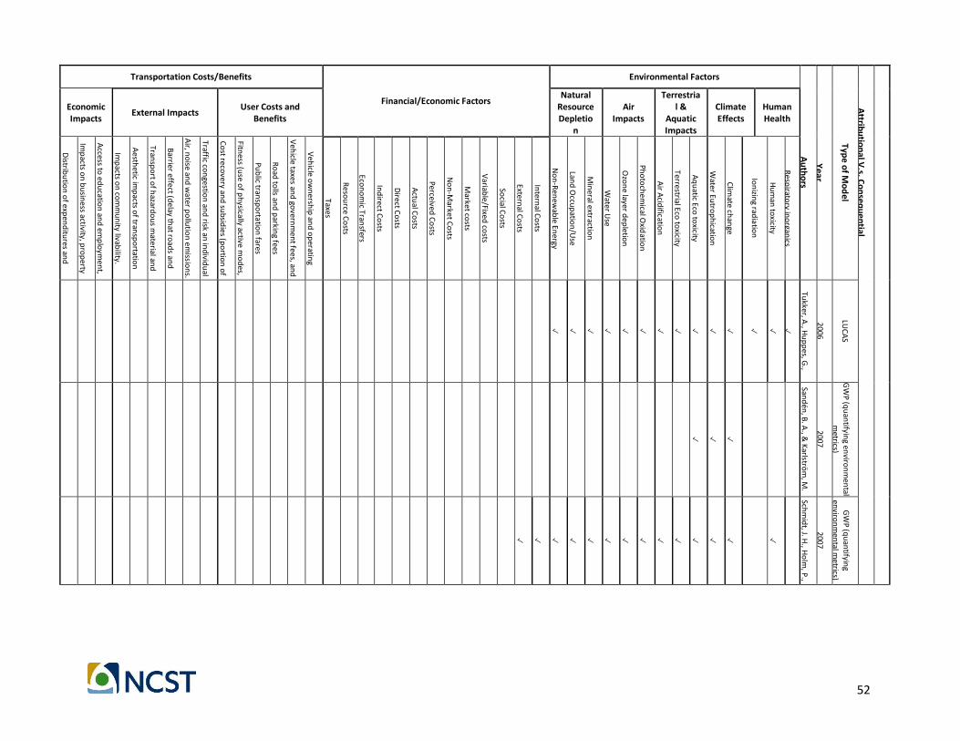
52

Attrib

utio

nal V

.s. Co

nseq

uen

tial

Type o

f Mo

del

Year

Au

tho

rs

Environmental Factors

Financial/Economic Factors

Transportation Costs/Benefits

Human Health

Climate Effects

Terrestrial &

Aquatic Impacts

Air Impacts

Natural Resource Depletio

n

User Costs and Benefits

External Impacts Economic Impacts

Resp

iratory in

organ

ics

Hu

man

toxicity

Ion

izing rad

iation

Clim

ate chan

ge

Water Eu

trop

hicatio

n

Aq

uatic Eco

toxicity

Terrestrial Eco to

xicity

Air A

cidificatio

n

Pho

toch

emical O

xidatio

n

Ozo

ne layer d

epletio

n

Water U

se

Min

eral extraction

Land

Occu

patio

n/U

se

No

n-R

enew

able En

ergy

Intern

al Co

sts

External C

osts

Social C

osts

Variab

le/Fixed co

sts

Market co

sts

No

n-M

arket Co

sts

Perceived C

osts

Actu

al Co

sts

Direct C

osts

Ind

irect Co

sts

Econ

om

ic Transfers

Reso

urce C

osts

Taxes

Veh

icle ow

nersh

ip an

d o

peratin

g exp

ense

s. V

ehicle taxes an

d go

vernm

ent fee

s, and

fu

el taxes. R

oad

tolls an

d p

arking fee

s

Pub

lic transp

ortatio

n fares

Fitness (u

se o

f ph

ysically active mo

des,

such

as walkin

g and

cycling).

Co

st recovery an

d su

bsidies (p

ortio

n o

f co

sts bo

rne b

y a particu

lar activity or

grou

p).

Traffic con

gestion

and

risk an in

divid

ual

or veh

icle class imp

ose

s on

oth

er road

u

sers.

Air, n

oise

and

water p

ollu

tion

emissio

ns.

Barrier effect (d

elay that ro

ads an

d

railroad

s cause

to n

on

mo

torized

travel). Tran

spo

rt of h

azardo

us m

aterial and

disp

osal o

f hazard

ou

s waste.

Aesth

etic imp

acts of tran

spo

rtation

facilities an

d traffic activity.

Imp

acts on

com

mu

nity livab

ility.

Access to

edu

cation

and

emp

loym

ent,

and

therefo

re econo

mic o

pp

ortu

nities.

Imp

acts on

bu

siness activity, p

rop

erty

values, an

d eco

no

mic d

evelop

men

t in an

area.

Distrib

utio

n o

f expen

ditu

res and

em

plo

ymen

t

LUC

AS

2006

Tukker, A

., Hu

pp

es, G.,

Gu

inée

, J., Heiju

ngs, R

., de

Ko

nin

g, A., van

Oers, L., . . .

Janse

n, B

.

✓

✓

✓

✓

✓

✓

✓

✓

✓

✓

✓

✓

✓

✓

GW

P (q

uan

tifying en

viron

men

tal m

etrics)

2007

Sand

én, B

. A., &

Karlströ

m, M

. ✓

✓

✓

GW

P (q

uan

tifying

enviro

nm

ental m

etrics)

2007

Schm

idt, J. H

., Ho

lm, P.,

Me

rrild, A

., &

Ch

ristense

n, P.

✓ ✓

✓

✓

✓

✓

✓

✓

✓

✓

✓

✓

✓

✓

53

Attrib

utio

nal V

.s. Co

nseq

uen

tial

Type o

f Mo

del

Year

Au

tho

rs

Environmental Factors

Financial/Economic Factors

Transportation Costs/Benefits

Human Health

Climate Effects

Terrestrial &

Aquatic Impacts

Air Impacts

Natural Resource Depletio

n

User Costs and Benefits

External Impacts Economic Impacts

Resp

iratory in

organ

ics

Hu

man

toxicity

Ion

izing rad

iation

Clim

ate chan

ge

Water Eu

trop

hicatio

n

Aq

uatic Eco

toxicity

Terrestrial Eco to

xicity

Air A

cidificatio

n

Pho

toch

emical O

xidatio

n

Ozo

ne layer d

epletio

n

Water U

se

Min

eral extraction

Land

Occu

patio

n/U

se

No

n-R

enew

able En

ergy

Intern

al Co

sts

External C

osts

Social C

osts

Variab

le/Fixed co

sts

Market co

sts

No

n-M

arket Co

sts

Perceived C

osts

Actu

al Co

sts

Direct C

osts

Ind

irect Co

sts

Econ

om

ic Transfers

Reso

urce C

osts

Taxes

Veh

icle ow

nersh

ip an

d o

peratin

g exp

ense

s. V

ehicle taxes an

d go

vernm

ent fee

s, and

fu

el taxes. R

oad

tolls an

d p

arking fee

s

Pub

lic transp

ortatio

n fares

Fitness (u

se o

f ph

ysically active mo

des,

such

as walkin

g and

cycling).

Co

st recovery an

d su

bsidies (p

ortio

n o

f co

sts bo

rne b

y a particu

lar activity or

grou

p).

Traffic con

gestion

and

risk an in

divid

ual

or veh

icle class imp

ose

s on

oth

er road

u

sers.

Air, n

oise

and

water p

ollu

tion

emissio

ns.

Barrier effect (d

elay that ro

ads an

d

railroad

s cause

to n

on

mo

torized

travel). Tran

spo

rt of h

azardo

us m

aterial and

disp

osal o

f hazard

ou

s waste.

Aesth

etic imp

acts of tran

spo

rtation

facilities an

d traffic activity.

Imp

acts on

com

mu

nity livab

ility.

Access to

edu

cation

and

emp

loym

ent,

and

therefo

re econo

mic o

pp

ortu

nities.

Imp

acts on

bu

siness activity, p

rop

erty

values, an

d eco

no

mic d

evelop

men

t in an

area.

Distrib

utio

n o

f expen

ditu

res and

em

plo

ymen

t

GW

P (q

uan

tifying

enviro

nm

ental m

etrics)

2008

Searchin

ger, T., Heim

lich, R

., H

ou

ghto

n, R

. A., D

on

g, F., Elo

beid

, A., Fab

iosa, J., . . . Yu

, T.-H

.

✓

✓

✓

✓

✓

✓

✓

✓

✓

✓

✓

✓

allocatio

n, w

aste man

agemen

t, p

aper recyclin

g, waste

incin

eration

1999

Ekvall, T. ✓ ✓

✓

✓

✓

✓

✓

✓

✓

✓

Co

nse

qu

ential LC

A

Partial equ

ilibriu

m

mo

del

2006

Ekvall, T., & A

nd

rae, A.

✓

54

Attrib

utio

nal V

.s. Co

nseq

uen

tial

Type o

f Mo

del

Year

Au

tho

rs

Environmental Factors

Financial/Economic Factors

Transportation Costs/Benefits

Human Health

Climate Effects

Terrestrial &

Aquatic Impacts

Air Impacts

Natural Resource Depletio

n

User Costs and Benefits

External Impacts Economic Impacts

Resp

iratory in

organ

ics

Hu

man

toxicity

Ion

izing rad

iation

Clim

ate chan

ge

Water Eu

trop

hicatio

n

Aq

uatic Eco

toxicity

Terrestrial Eco to

xicity

Air A

cidificatio

n

Pho

toch

emical O

xidatio

n

Ozo

ne layer d

epletio

n

Water U

se

Min

eral extraction

Land

Occu

patio

n/U

se

No

n-R

enew

able En

ergy

Intern

al Co

sts

External C

osts

Social C

osts

Variab

le/Fixed co

sts

Market co

sts

No

n-M

arket Co

sts

Perceived C

osts

Actu

al Co

sts

Direct C

osts

Ind

irect Co

sts

Econ

om

ic Transfers

Reso

urce C

osts

Taxes

Veh

icle ow

nersh

ip an

d o

peratin

g exp

ense

s. V

ehicle taxes an

d go

vernm

ent fee

s, and

fu

el taxes. R

oad

tolls an

d p

arking fee

s

Pub

lic transp

ortatio

n fares

Fitness (u

se o

f ph

ysically active mo

des,

such

as walkin

g and

cycling).

Co

st recovery an

d su

bsidies (p

ortio

n o

f co

sts bo

rne b

y a particu

lar activity or

grou

p).

Traffic con

gestion

and

risk an in

divid

ual

or veh

icle class imp

ose

s on

oth

er road

u

sers.

Air, n

oise

and

water p

ollu

tion

emissio

ns.

Barrier effect (d

elay that ro

ads an

d

railroad

s cause

to n

on

mo

torized

travel). Tran

spo

rt of h

azardo

us m

aterial and

disp

osal o

f hazard

ou

s waste.

Aesth

etic imp

acts of tran

spo

rtation

facilities an

d traffic activity.

Imp

acts on

com

mu

nity livab

ility.

Access to

edu

cation

and

emp

loym

ent,

and

therefo

re econo

mic o

pp

ortu

nities.

Imp

acts on

bu

siness activity, p

rop

erty

values, an

d eco

no

mic d

evelop

men

t in an

area.

Distrib

utio

n o

f expen

ditu

res and

em

plo

ymen

t

The Eco

-ind

icator 99 Im

pact

categories

2000

Go

edkoo

p, M

., & Sp

riensm

a, R.

✓

✓

✓

✓

✓

✓

✓

✓

✓

✓

✓

✓

✓

✓

The Eco

-ind

icator 99 Im

pact

categories

1998

Go

edkoo

p, M

., Ho

fstetter, P., M

üller-W

en

k, R., &

Sp

riemsm

a, R.

✓

✓

✓

✓

✓

✓

✓

✓

✓

✓

✓

✓

✓

✓

ReC

ipe M

od

el

2009

Go

edkoo

p, M

., Heiju

ngs, R

., H

uijb

regts, M., D

e Schryver,

A., Stru

ijs, J., & V

an Zelm

, R.

✓

✓

✓

✓

✓

✓

✓

✓

✓

✓

✓

✓

✓

✓

Bio

energy

systems

2011

Ch

erub

ini, F.,

& Strø

mm

an,

A. H

.

✓ ✓

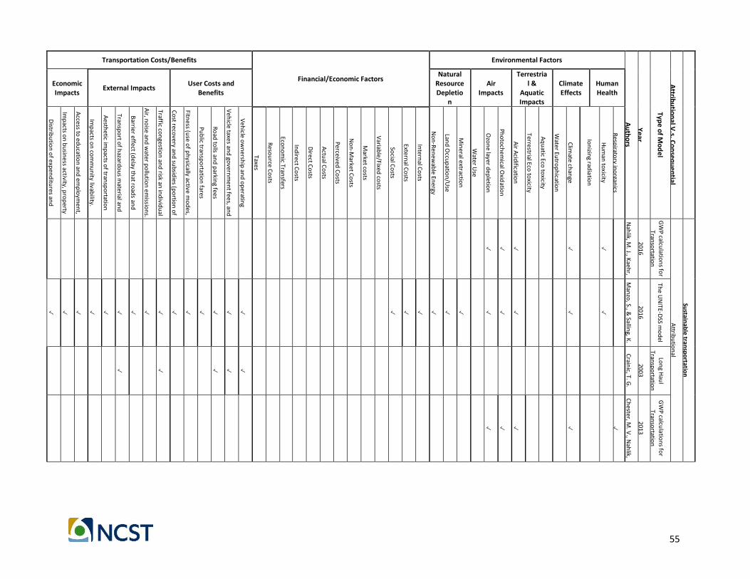
55

Attrib

utio

nal V

.s. Co

nseq

uen

tial

Type o

f Mo

del

Year

Au

tho

rs

Environmental Factors

Financial/Economic Factors

Transportation Costs/Benefits

Human Health

Climate Effects

Terrestrial &

Aquatic Impacts

Air Impacts

Natural Resource Depletio

n

User Costs and Benefits

External Impacts Economic Impacts

Resp

iratory in

organ

ics

Hu

man

toxicity

Ion

izing rad

iation

Clim

ate chan

ge

Water Eu

trop

hicatio

n

Aq

uatic Eco

toxicity

Terrestrial Eco to

xicity

Air A

cidificatio

n

Pho

toch

emical O

xidatio

n

Ozo

ne layer d

epletio

n

Water U

se

Min

eral extraction

Land

Occu

patio

n/U

se

No

n-R

enew

able En

ergy

Intern

al Co

sts

External C

osts

Social C

osts

Variab

le/Fixed co

sts

Market co

sts

No

n-M

arket Co

sts

Perceived C

osts

Actu

al Co

sts

Direct C

osts

Ind

irect Co

sts

Econ

om

ic Transfers

Reso

urce C

osts

Taxes

Veh

icle ow

nersh

ip an

d o

peratin

g exp

ense

s. V

ehicle taxes an

d go

vernm

ent fee

s, and

fu

el taxes. R

oad

tolls an

d p

arking fee

s

Pub

lic transp

ortatio

n fares

Fitness (u

se o

f ph

ysically active mo

des,

such

as walkin

g and

cycling).

Co

st recovery an

d su

bsidies (p

ortio

n o

f co

sts bo

rne b

y a particu

lar activity or

grou

p).

Traffic con

gestion

and

risk an in

divid

ual

or veh

icle class imp

ose

s on

oth

er road

u

sers.

Air, n

oise

and

water p

ollu

tion

emissio

ns.

Barrier effect (d

elay that ro

ads an

d

railroad

s cause

to n

on

mo

torized

travel). Tran

spo

rt of h

azardo

us m

aterial and

disp

osal o

f hazard

ou

s waste.

Aesth

etic imp

acts of tran

spo

rtation

facilities an

d traffic activity.

Imp

acts on

com

mu

nity livab

ility.

Access to

edu

cation

and

emp

loym

ent,

and

therefo

re econo

mic o

pp

ortu

nities.

Imp

acts on

bu

siness activity, p

rop

erty

values, an

d eco

no

mic d

evelop

men

t in an

area.

Distrib

utio

n o

f expen

ditu

res and

em

plo

ymen

t

Sustain

able

tran

spo

rtation

Attrib

utio

nal

GW

P calcu

lation

s for

Transo

rtation

2016

Nah

lik, M. J., K

aehr,

A. T., C

hester, M

. V.,

Ho

rvath, A

., &

Taptich

, M. N

.

✓ ✓ ✓

✓

✓

The U

NITE

-DSS m

od

el

2016

Man

zo, S., &

Salling, K

. B

.

✓ ✓ ✓

✓

✓ ✓

✓

✓

✓

✓

✓ ✓

✓

✓

✓

✓

✓

✓

✓

✓

✓

✓

✓

✓

✓

✓

Lon

g Hau

l Tran

spo

rtation

2003

Crain

ic, T. G.

✓

✓

✓ ✓ ✓

GW

P calcu

lation

s for

Transo

rtation

2013

Ch

ester, M. V

., Nah

lik, M

. J., Fraser, A

. M.,

Kim

ball, M

. A., &

G

arikapati, V

. M.

✓ ✓ ✓

✓

✓

56

Attrib

utio

nal V

.s. Co

nseq

uen

tial

Type o

f Mo

del

Year

Au

tho

rs

Environmental Factors

Financial/Economic Factors

Transportation Costs/Benefits

Human Health

Climate Effects

Terrestrial &

Aquatic Impacts

Air Impacts

Natural Resource Depletio

n

User Costs and Benefits

External Impacts Economic Impacts

Resp

iratory in

organ

ics

Hu

man

toxicity

Ion

izing rad

iation

Clim

ate chan

ge

Water Eu

trop

hicatio

n

Aq

uatic Eco

toxicity

Terrestrial Eco to

xicity

Air A

cidificatio

n

Pho

toch

emical O

xidatio

n

Ozo

ne layer d

epletio

n

Water U

se

Min

eral extraction

Land

Occu

patio

n/U

se

No

n-R

enew

able En

ergy

Intern

al Co

sts

External C

osts

Social C

osts

Variab

le/Fixed co

sts

Market co

sts

No

n-M

arket Co

sts

Perceived C

osts

Actu

al Co

sts

Direct C

osts

Ind

irect Co

sts

Econ

om

ic Transfers

Reso

urce C

osts

Taxes

Veh

icle ow

nersh

ip an

d o

peratin

g exp

ense

s. V

ehicle taxes an

d go

vernm

ent fee

s, and

fu

el taxes. R

oad

tolls an

d p

arking fee

s

Pub

lic transp

ortatio

n fares

Fitness (u

se o

f ph

ysically active mo

des,

such

as walkin

g and

cycling).

Co

st recovery an

d su

bsidies (p

ortio

n o

f co

sts bo

rne b

y a particu

lar activity or

grou

p).

Traffic con

gestion

and

risk an in

divid

ual

or veh

icle class imp

ose

s on

oth

er road

u

sers.

Air, n

oise

and

water p

ollu

tion

emissio

ns.

Barrier effect (d

elay that ro

ads an

d

railroad

s cause

to n

on

mo

torized

travel). Tran

spo

rt of h

azardo

us m

aterial and

disp

osal o

f hazard

ou

s waste.

Aesth

etic imp

acts of tran

spo

rtation

facilities an

d traffic activity.

Imp

acts on

com

mu

nity livab

ility.

Access to

edu

cation

and

emp

loym

ent,

and

therefo

re econo

mic o

pp

ortu

nities.

Imp

acts on

bu

siness activity, p

rop

erty

values, an

d eco

no

mic d

evelop

men

t in an

area.

Distrib

utio

n o

f expen

ditu

res and

em

plo

ymen

t

Energy U

se (Private v.s.

Pub

lic Transit)

2010

Ch

ester, M. V

., Ho

rvath,

A., &

Mad

anat, S.

✓ ✓

✓ ✓ ✓

✓

✓

✓ ✓

✓

Energy C

on

sum

ptio

n-G

WP

2010

Ch

ester, M., &

Ho

rvath, A

. ✓ ✓

✓

✓ ✓ ✓

✓

Energy C

on

sum

ptio

n-G

WP

2012

Ch

ester, M., &

Ho

rvath, A

. ✓ ✓

✓

✓ ✓ ✓

✓

✓

✓

✓

✓

✓

✓

✓

Co

st An

alysis

LCC

###

Langd

on

, D.

✓ ✓

✓

✓

✓

✓

✓

✓

✓

✓

✓

✓

✓

✓

✓ ✓

✓

57

Attrib

utio

nal V

.s. Co

nseq

uen

tial

Type o

f Mo

del

Year

Au

tho

rs

Environmental Factors

Financial/Economic Factors

Transportation Costs/Benefits

Human Health

Climate Effects

Terrestrial &

Aquatic Impacts

Air Impacts

Natural Resource Depletio

n

User Costs and Benefits

External Impacts Economic Impacts

Resp

iratory in

organ

ics

Hu

man

toxicity

Ion

izing rad

iation

Clim

ate chan

ge

Water Eu

trop

hicatio

n

Aq

uatic Eco

toxicity

Terrestrial Eco to

xicity

Air A

cidificatio

n

Pho

toch

emical O

xidatio

n

Ozo

ne layer d

epletio

n

Water U

se

Min

eral extraction

Land

Occu

patio

n/U

se

No

n-R

enew

able En

ergy

Intern

al Co

sts

External C

osts

Social C

osts

Variab

le/Fixed co

sts

Market co

sts

No

n-M

arket Co

sts

Perceived C

osts

Actu

al Co

sts

Direct C

osts

Ind

irect Co

sts

Econ

om

ic Transfers

Reso

urce C

osts

Taxes

Veh

icle ow

nersh

ip an

d o

peratin

g exp

ense

s. V

ehicle taxes an

d go

vernm

ent fee

s, and

fu

el taxes. R

oad

tolls an

d p

arking fee

s

Pub

lic transp

ortatio

n fares

Fitness (u

se o

f ph

ysically active mo

des,

such

as walkin

g and

cycling).

Co

st recovery an

d su

bsidies (p

ortio

n o

f co

sts bo

rne b

y a particu

lar activity or

grou

p).

Traffic con

gestion

and

risk an in

divid

ual

or veh

icle class imp

ose

s on

oth

er road

u

sers.

Air, n

oise

and

water p

ollu

tion

emissio

ns.

Barrier effect (d

elay that ro

ads an

d

railroad

s cause

to n

on

mo

torized

travel). Tran

spo

rt of h

azardo

us m

aterial and

disp

osal o

f hazard

ou

s waste.

Aesth

etic imp

acts of tran

spo

rtation

facilities an

d traffic activity.

Imp

acts on

com

mu

nity livab

ility.

Access to

edu

cation

and

emp

loym

ent,

and

therefo

re econo

mic o

pp

ortu

nities.

Imp

acts on

bu

siness activity, p

rop

erty

values, an

d eco

no

mic d

evelop

men

t in an

area.

Distrib

utio

n o

f expen

ditu

res and

em

plo

ymen

t

UN

ITE-D

SS m

od

el

###

Salling, K

. B.,

& Leleu

r, S. ✓

✓ ✓

✓

GW

P (q

uan

tifying en

viron

men

tal m

etrics)

2007

Ku

osm

anen

, T., & K

ortelain

en, M

. ✓

✓

✓ ✓ ✓

✓

✓

✓

Econ

om

ic Inp

ut/O

utp

ut

An

alysis

1995

Co

bas, E., H

end

rickson

, C.,

Lave, L., & M

cMich

ael, F. ✓

✓

✓

✓

✓

✓

✓ ✓

WT

P & C

OI eco

no

mic

Mo

del

###

Alb

erini, A

., & K

rup

nick, A

.

✓ ✓

✓

✓ ✓

✓ ✓ ✓

✓

✓ ✓ ✓ ✓ ✓

58

Attrib

utio

nal V

.s. Co

nseq

uen

tial

Type o

f Mo

del

Year

Au

tho

rs

Environmental Factors

Financial/Economic Factors

Transportation Costs/Benefits

Human Health

Climate Effects

Terrestrial &

Aquatic Impacts

Air Impacts

Natural Resource Depletio

n

User Costs and Benefits

External Impacts Economic Impacts

Resp

iratory in

organ

ics

Hu

man

toxicity

Ion

izing rad

iation

Clim

ate chan

ge

Water Eu

trop

hicatio

n

Aq

uatic Eco

toxicity

Terrestrial Eco to

xicity

Air A

cidificatio

n

Pho

toch

emical O

xidatio

n

Ozo

ne layer d

epletio

n

Water U

se

Min

eral extraction

Land

Occu

patio

n/U

se

No

n-R

enew

able En

ergy

Intern

al Co

sts

External C

osts

Social C

osts

Variab

le/Fixed co

sts

Market co

sts

No

n-M

arket Co

sts

Perceived C

osts

Actu

al Co

sts

Direct C

osts

Ind

irect Co

sts

Econ

om

ic Transfers

Reso

urce C

osts

Taxes

Veh

icle ow

nersh

ip an

d o

peratin

g exp

ense

s. V

ehicle taxes an

d go

vernm

ent fee

s, and

fu

el taxes. R

oad

tolls an

d p

arking fee

s

Pub

lic transp

ortatio

n fares

Fitness (u

se o

f ph

ysically active mo

des,

such

as walkin

g and

cycling).

Co

st recovery an

d su

bsidies (p

ortio

n o

f co

sts bo

rne b

y a particu

lar activity or

grou

p).

Traffic con

gestion

and

risk an in

divid

ual

or veh

icle class imp

ose

s on

oth

er road

u

sers.

Air, n

oise

and

water p

ollu

tion

emissio

ns.

Barrier effect (d

elay that ro

ads an

d

railroad

s cause

to n

on

mo

torized

travel). Tran

spo

rt of h

azardo

us m

aterial and

disp

osal o

f hazard

ou

s waste.

Aesth

etic imp

acts of tran

spo

rtation

facilities an

d traffic activity.

Imp

acts on

com

mu

nity livab

ility.

Access to

edu

cation

and

emp

loym

ent,

and

therefo

re econo

mic o

pp

ortu

nities.

Imp

acts on

bu

siness activity, p

rop

erty

values, an

d eco

no

mic d

evelop

men

t in an

area.

Distrib

utio

n o

f expen

ditu

res and

em

plo

ymen

t

cost-B

enfit M

od

els (HER

S, StratB

ENC

OST, STEA

M)

1999

Bailly, H

., & B

rinckerh

off, P.

✓

✓ ✓

✓

✓ ✓

✓ ✓

✓ ✓ ✓

✓ ✓

✓

✓ ✓ ✓

✓

✓

✓ ✓

Econ

om

ic Inp

ut/O

utp

ut

An

alysis

2001

No

rris, G. A

. ✓

✓ ✓

✓

ME

MA

and

PEMA

2002

Bu

rritt, R. L., H

ahn

, T., & Sch

altegger, S.

✓ ✓

59

Attrib

utio

nal V

.s. Co

nseq

uen

tial

Type o

f Mo

del

Year

Au

tho

rs

Environmental Factors

Financial/Economic Factors

Transportation Costs/Benefits

Human Health

Climate Effects

Terrestrial &

Aquatic Impacts

Air Impacts

Natural Resource Depletio

n

User Costs and Benefits

External Impacts Economic Impacts

Resp

iratory in

organ

ics

Hu

man

toxicity

Ion

izing rad

iation

Clim

ate chan

ge

Water Eu

trop

hicatio

n

Aq

uatic Eco

toxicity

Terrestrial Eco to

xicity

Air A

cidificatio

n

Pho

toch

emical O

xidatio

n

Ozo

ne layer d

epletio

n

Water U

se

Min

eral extraction

Land

Occu

patio

n/U

se

No

n-R

enew

able En

ergy

Intern

al Co

sts

External C

osts

Social C

osts

Variab

le/Fixed co

sts

Market co

sts

No

n-M

arket Co

sts

Perceived C

osts

Actu

al Co

sts

Direct C

osts

Ind

irect Co

sts

Econ

om

ic Transfers

Reso

urce C

osts

Taxes

Veh

icle ow

nersh

ip an

d o

peratin

g exp

ense

s. V

ehicle taxes an

d go

vernm

ent fee

s, and

fu

el taxes. R

oad

tolls an

d p

arking fee

s

Pub

lic transp

ortatio

n fares

Fitness (u

se o

f ph

ysically active mo

des,

such

as walkin

g and

cycling).

Co

st recovery an

d su

bsidies (p

ortio

n o

f co

sts bo

rne b

y a particu

lar activity or

grou

p).

Traffic con

gestion

and

risk an in

divid

ual

or veh

icle class imp

ose

s on

oth

er road

u

sers.

Air, n

oise

and

water p

ollu

tion

emissio

ns.

Barrier effect (d

elay that ro

ads an

d

railroad

s cause

to n

on

mo

torized

travel). Tran

spo

rt of h

azardo

us m

aterial and

disp

osal o

f hazard

ou

s waste.

Aesth

etic imp

acts of tran

spo

rtation

facilities an

d traffic activity.

Imp

acts on

com

mu

nity livab

ility.

Access to

edu

cation

and

emp

loym

ent,

and

therefo

re econo

mic o

pp

ortu

nities.

Imp

acts on

bu

siness activity, p

rop

erty

values, an

d eco

no

mic d

evelop

men

t in an

area.

Distrib

utio

n o

f expen

ditu

res and

em

plo

ymen

t

Energy System

s

Attrib

utio

nal

Energy In

put/O

utp

ut

Mo

delin

g

2017

ww

w.Led

vance.co

m

✓

✓ ✓

✓

Energy In

put/O

utp

ut

Mo

delin

g

2006

Berglu

nd

, M., &

Bö

rjesson

, P. ✓ ✓ ✓ ✓ ✓

Energy In

put/O

utp

ut

Mo

delin

g

2008

Allen

, S., Ham

mo

nd

, G.,

& M

cMan

us, M

. ✓ ✓

✓

✓

✓ ✓

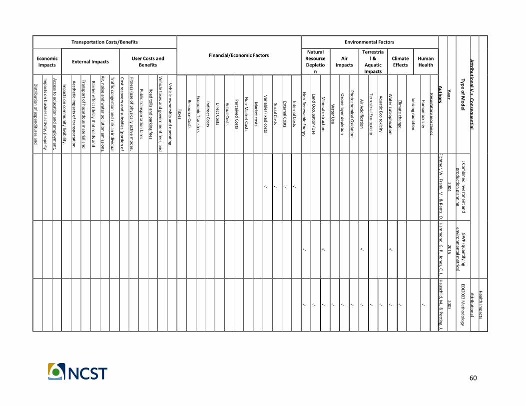
60

Attrib

utio

nal V

.s. Co

nseq

uen

tial

Type o

f Mo

del

Year

Au

tho

rs

Environmental Factors

Financial/Economic Factors

Transportation Costs/Benefits

Human Health

Climate Effects

Terrestrial &

Aquatic Impacts

Air Impacts

Natural Resource Depletio

n

User Costs and Benefits

External Impacts Economic Impacts

Resp

iratory in

organ

ics

Hu

man

toxicity

Ion

izing rad

iation

Clim

ate chan

ge

Water Eu

trop

hicatio

n

Aq

uatic Eco

toxicity

Terrestrial Eco to

xicity

Air A

cidificatio

n

Pho

toch

emical O

xidatio

n

Ozo

ne layer d

epletio

n

Water U

se

Min

eral extraction

Land

Occu

patio

n/U

se

No

n-R

enew

able En

ergy

Intern

al Co

sts

External C

osts

Social C

osts

Variab

le/Fixed co

sts

Market co

sts

No

n-M

arket Co

sts

Perceived C

osts

Actu

al Co

sts

Direct C

osts

Ind

irect Co

sts

Econ

om

ic Transfers

Reso

urce C

osts

Taxes

Veh

icle ow

nersh

ip an

d o

peratin

g exp

ense

s. V

ehicle taxes an

d go

vernm

ent fee

s, and

fu

el taxes. R

oad

tolls an

d p

arking fee

s

Pub

lic transp

ortatio

n fares

Fitness (u

se o

f ph

ysically active mo

des,

such

as walkin

g and

cycling).

Co

st recovery an

d su

bsidies (p

ortio

n o

f co

sts bo

rne b

y a particu

lar activity or

grou

p).

Traffic con

gestion

and

risk an in

divid

ual

or veh

icle class imp

ose

s on

oth

er road

u

sers.

Air, n

oise

and

water p

ollu

tion

emissio

ns.

Barrier effect (d

elay that ro

ads an

d

railroad

s cause

to n

on

mo

torized

travel). Tran

spo

rt of h

azardo

us m

aterial and

disp

osal o

f hazard

ou

s waste.

Aesth

etic imp

acts of tran

spo

rtation

facilities an

d traffic activity.

Imp

acts on

com

mu

nity livab

ility.

Access to

edu

cation

and

emp

loym

ent,

and

therefo

re econo

mic o

pp

ortu

nities.

Imp

acts on

bu

siness activity, p

rop

erty

values, an

d eco

no

mic d

evelop

men

t in an

area.

Distrib

utio

n o

f expen

ditu

res and

em

plo

ymen

t

: Co

mb

ined

investm

ent an

d

pro

du

ction

plan

nin

g

2004

Fichtn

er, W., Fran

k, M., &

Ren

tz, O.

✓

✓

✓

✓

GW

P (q

uan

tifying

enviro

nm

ental m

etrics)

2015

Ham

mo

nd

, G. P., Jo

nes, C

. I., &

O'G

rady, Á

. ✓ ✓ ✓ ✓

Health

Imp

acts

Attrib

utio

nal

EDI2003 M

eth

od

olo

gy

2005

Hau

schild

, M., &

Pottin

g, J. ✓ ✓

✓

✓

✓

✓

✓

✓

✓

✓

✓

✓

61

Attrib

utio

nal V

.s. Co

nseq

uen

tial

Type o

f Mo

del

Year

Au

tho

rs

Environmental Factors

Financial/Economic Factors

Transportation Costs/Benefits

Human Health

Climate Effects

Terrestrial &

Aquatic Impacts

Air Impacts

Natural Resource Depletio

n

User Costs and Benefits

External Impacts Economic Impacts

Resp

iratory in

organ

ics

Hu

man

toxicity

Ion

izing rad

iation

Clim

ate chan

ge

Water Eu

trop

hicatio

n

Aq

uatic Eco

toxicity

Terrestrial Eco to

xicity

Air A

cidificatio

n

Pho

toch

emical O

xidatio

n

Ozo

ne layer d

epletio

n

Water U

se

Min

eral extraction

Land

Occu

patio

n/U

se

No

n-R

enew

able En

ergy

Intern

al Co

sts

External C

osts

Social C

osts

Variab

le/Fixed co

sts

Market co

sts

No

n-M

arket Co

sts

Perceived C

osts

Actu

al Co

sts

Direct C

osts

Ind

irect Co

sts

Econ

om

ic Transfers

Reso

urce C

osts

Taxes

Veh

icle ow

nersh

ip an

d o

peratin

g exp

ense

s. V

ehicle taxes an

d go

vernm

ent fee

s, and

fu

el taxes. R

oad

tolls an

d p

arking fee

s

Pub

lic transp

ortatio

n fares

Fitness (u

se o

f ph

ysically active mo

des,

such

as walkin

g and

cycling).

Co

st recovery an

d su

bsidies (p

ortio

n o

f co

sts bo

rne b

y a particu

lar activity or

grou

p).

Traffic con

gestion

and

risk an in

divid

ual

or veh

icle class imp

ose

s on

oth

er road

u

sers.

Air, n

oise

and

water p

ollu

tion

emissio

ns.

Barrier effect (d

elay that ro

ads an

d

railroad

s cause

to n

on

mo

torized

travel). Tran

spo

rt of h

azardo

us m

aterial and

disp

osal o

f hazard

ou

s waste.

Aesth

etic imp

acts of tran

spo

rtation

facilities an

d traffic activity.

Imp

acts on

com

mu

nity livab

ility.

Access to

edu

cation

and

emp

loym

ent,

and

therefo

re econo

mic o

pp

ortu

nities.

Imp

acts on

bu

siness activity, p

rop

erty

values, an

d eco

no

mic d

evelop

men

t in an

area.

Distrib

utio

n o

f expen

ditu

res and

em

plo

ymen

t

Health

Imp

act assessm

ent

2011

Bo

ard, T. R

., Natio

nal

Acad

emies o

f Scien

ces, E., &

Me

dicin

e

✓

✓

✓ ✓

Health

Imp

act assessm

ent

2015

Jolliet, O

., & Fan

tke, P. ( ✓

✓

✓

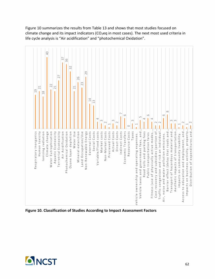
62

Figure 10 summarizes the results from Table 13 and shows that most studies focused on climate change and its impact indicators (CO2eq in most cases). The next most used criteria in life cycle analysis is “Air acidification” and “photochemical Oxidation”.

Figure 10. Classification of Studies According to Impact Assessment Factors

1921

1840

2221

2737

363

221

2623

2914

134

32

13

27

60

31

54

64

2 26

83 3

12

12

Re

sp

ira

tory

in

org

an

ics

Hu

ma

n t

ox

icit

yIo

niz

ing

ra

dia

tio

nC

lim

ate

ch

an

ge

Wa

ter

Eu

tro

ph

ica

tio

nA

qu

ati

c E

co

tox

icit

yT

err

etr

ial

Ec

oto

xic

ity

Air

Ac

idif

ica

tio

nP

ho

toc

he

mic

al

Ox

ida

tio

nO

zo

ne

la

ye

r d

ep

leti

on

Wa

ter

Us

eM

ine

ral

ex

tarc

tio

nL

an

d O

cc

up

ati

on

/U

se

No

n-R

en

ew

ab

le E

ne

rgy

Ex

tern

al

Co

sts

So

cia

l C

os

tsV

ari

ab

le/

Fix

ed

co

sts

Ma

rke

t c

os

tsN

on

-Ma

rke

t C

os

tsP

rec

iev

ed

Co

sts

Ac

tua

l C

os

tsD

ire

ct

Co

sts

Ind

ire

ct

Co

sts

Ec

on

om

ic T

ran

sfe

rsR

es

ou

rce

Co

sts

Ta

xe

sV

eh

icle

ow

ne

rsh

ip a

nd

op

era

tin

g e

xp

en

se

s.

Ve

hic

le t

ax

es

an

d g

ov

ern

me

nt

fee

s,

an

d …

Ro

ad

to

lls

an

d p

ark

ing

fe

es

Pu

bli

c t

ran

sp

ort

ati

on

fa

res

F

itn

es

s (

us

e o

f p

hy

sic

all

y a

cti

ve

mo

de

s, …

Co

st

rec

ov

ery

an

d s

ub

sid

ies

(p

ort

ion

of …

Tra

ffic

co

ng

es

tio

n a

nd

ris

k a

n i

nd

ivid

ua

l …A

ir,

no

ise

an

d w

ate

r p

oll

uti

on

em

iss

ion

s.

Ba

rrie

r e

ffe

ct

(de

lay

th

at

roa

ds

an

d …

Tra

ns

po

rt o

f h

az

ard

ou

s m

ate

ria

l a

nd

…A

es

the

tic

im

pa

cts

of

tra

ns

po

rta

tio

n …

Imp

ac

ts o

n c

om

mu

nit

y l

iva

bil

ity

. A

cc

es

s t

o e

du

ca

tio

n a

nd

em

plo

ym

en

t, a

nd

…Im

pa

cts

on

bu

sin

es

s a

cti

vit

y,

pro

pe

rty

…D

istr

ibu

tio

n o

f e

xp

en

dit

ure

s a

nd

…

63

VI. Freight System Conceptualization and Impact Asses Framework

The objective of the work is to develop a Freight System Conceptualization and Impact Assessment Framework of the freight movements in the State to identify the industry sectors and/or commodity types that have the largest impacts. The framework could assist in the decision-making process and the development of strategies to improve the system. The strategies could be in the form of regulatory actions, plans, or the implementation of specific infrastructure, operational, or technological projects. This is important considering that the California Sustainable Freight Action Plan (CSFAP) seeks to “… Improve freight system efficiency 25 percent by increasing the value of goods and services produced from the freight sector, relative to the amount of carbon that it produces by 2030...” (California Governor's Office, 2016). The metric considers the freight transportation sector as the establishments in the North American Industry Classification System (NAICS) codes 48 and 49 (minus transit and passenger transport). These industry sectors include establishments in the air, rail, water, truck, pipeline, and other transportation and support activities, as well as warehousing and storage. While these are the main transportation related establishments, there are a number of establishments not categorized in NAICS 48 and 49, which also transport cargo usually using their own fleets. These segments are not included in the defined CSFAP metric. Moreover, it is important to recognize that the transportation system, in many cases, does not add value to the products or services transported and is just the conduit between other components of supply chains and industries. The efficiency of the freight transportation system may not always result from the optimal selection of routes, vehicles and technologies, which directly relate to the transportation system, but from complex logistics activities (e.g., frequency of distribution, shipment size, and delivery options). Consequently, the proposed framework must be consistent with the types of decisions and the scope of the analysis (e.g., system wide, corridor, specific project, policy), and the objective (e.g., cost minimization, return on investment, social and health impacts, emission reductions, comparison between alternatives, impact assessment, cost assessment). With this in mind, the research team proposes a conceptual framework based on a LCA methodology. Although, LCA has incorporated costing in the LCC, social impacts in the S-LCA, and a combination of models in the LCSA frameworks, it is not fundamentally a cost-benefit framework. During the review process, the research team identified that Caltrans developed and uses the California Life-Cycle Benefit/Cost Analysis Model (CAL-B/C). At the project level (e.g., infrastructure investment, technology change), the tool is comprehensive (See Annex C for examples of model considerations). However, the life-cycle component of the tool may not incorporate the details of a complete LCIA framework. Moreover, the team found that California agencies have tested and used other benefit-cost tools such as TREDIS3. Therefore, the research team concentrated on developing the framework that expanded the LCA capabilities, and could serve as an input to the CAL-B/C. In doing so, the team built upon the

3 https://www.tredis.com/. TREDIS is a Benefit-Cost Analysis, Economic Impact Analysis, and Financial Impact Analysis tool for transportation planning.

64

framework developed by Nahlik et al. (2015) for the California Air Resources Board and earlier work by Facanha and Horvath (2006); Facanha and Horvath (2007). These works also focused on the freight originated from or destined to California at the aggregate level. The proposed framework in this project, explicitly considers the flows for different industries and commodity groups. Nevertheless, the team adapted some sections from Nahlik et al. (2015) framework. The proposed framework, as a stand-alone tool, seeks to produce impact assessments for the freight flows in the base case, and can estimate the impacts for a set of scenarios to do comparative analyses. Agencies could use other benefit-cost models to assess such scenarios. Considering the scope and complexity of such a framework, this section illustrates the main components using a high-level logical framework (see Figure 11). This high-level logical framework includes three main components that resemble the LCA phases: problem definition, goals, and system boundaries; measurement indicators and data collection; and impact categories, and analysis of results. One particular characteristic of the framework is that is it envisioned to cover end-to-end supply chains (which could span over multiple geographic boundaries, various industry sectors, and commodity types). The team suggests the use of the supply chain characterization in Table 2 as a guide to understand the type of freight activities carried out by key supply chains in the study area. This would help understand the limitations of the framework implementation, and aid in the data gathering and collection process.

Figure 11. Logical Framework Figure 12 illustrates the main considerations when defining the problem, and setting the goal and scope of the analyses. For instance, when analyzing supply chains, will the estimates include all components, or just the transportation related activities? The functional unit is another important decision, as it will determine its usability in other models such as the benefit-cost models. Previous research studies have used moving a metric ton of cargo over a mile distance as the functional unit. The boundary and scope would also affect the implementation of the framework.

Problem definition, goals, system boundaries

Defining measurement indicators, data collection

(inputs)

Defining impact categories, clasification systems, normalization

and result interpretation

65

Figure 12. Goal and Scope Recalling Section II in this document, several modes of transportation or services move freight such as trucking, air, rail, and water (inland waterways, ocean shipping). Therefore, the LCA must include life cycles over these modes, as well as the infrastructure used. Chester (2015) defines a number of life cycle groupings for freight (see Table 14). For each of the groupings, the vehicle and infrastructure could include manufacturing or construction, operation, maintenance and end-of-life (not included in Table 14) phases. The research team found that there is a general lack of information and methods to consider all these phases, especially in terms of infrastructure. While there are databases (see Annex A) that provide some information for the use phases for the vehicle, and energy production, there is a lack of data and allocation methods for infrastructure, especially maintenance and pavement. Figure 13 shows some examples of the freight transportation services, and the potential types of vehicles considered when conducting the analyses. Depending on the type of services and the type of analyses, the implementation of the framework requires further considerations in terms of measurement indicators for the transportation system (e.g., flows, costs, service reliability).

66

Figure 14 illustrates the type of data necessary as input to conduct the analyses, and potential data sources for process inventories for the various life cycle groupings. Data collection and assembly are very time consuming. In some cases, flow inventories exist for the various vehicles, or infrastructures; in other cases, the inventories have to be constructed based on individual flows. In California, the Air Resources Board have developed tools for emissions inventories (see https://www.arb.ca.gov/msei/categories.htm). For instance, CARB uses EMFAC model to assess emissions from on-road vehicles. Other commonly used models include the Argonne National Laboratory’s Greenhouse gases, Regulated Emissions, and Energy use in Transportation (GREET®) Model. Table 14. Freight Life Cycles

Note: APU = Auxiliary Power Unit Source: (Chester, 2015)

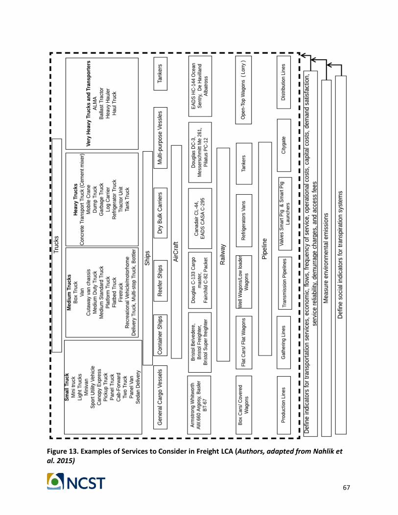
67

Figure 13. Examples of Services to Consider in Freight LCA (Authors, adapted from Nahlik et al. 2015)

68

The inventories and inputs generate a number of results such as atmospheric and waterborne emissions, solid waste, and if included, costs for the functional unit. The framework implementation also requires defining the impact categories; there are different models representing impact assessment methodologies and each of them may consider different factors (see Annex B for examples). The following are examples of frequently used impact categories. Human Toxicity Potential (HTP)

The main goal of this category is to indicate the chemical and environmental consequences of a processor product to human health. Examples of this category are sodium dichromate, and hydrogen fluoride, mostly generated from electricity production from fossil fuels. Such chemicals can harm human race through inhalation, touch, and ingestion (Hertwich et al., 2001). Global Warming Potential (GWP)

One of the most popular categories in order to represent impact categories is through Global Warming Potential (GWP). This factor indicates the amount of greenhouse gas emissions (e.g. CO2, CH4) released in to the environment from a product or process. This factor is calculated for a 100-year time horizon and its represented in a CO2 equivalent (www.Ledvance.com, 2017). Acidification Potential (AP)

This category of impact assessment refers to the lack of certain chemical nutrient in an ecosystem including calcium, magnesium, and potassium. Due to this loss, the acid elements are replaced and result in atmospheric pollution. Acid rain and its consequent effects on environment is an example of this category. The acidification Potential mostly happen due to the replacement of NO2 and SO2 and represents as SO2 equivalent (www.Ledvance.com, 2017). Eutrophication Potential (EP)

Due to the concentration of chemicals into an ecosystem eutrophication happens. These chemicals are mainly nitrogen and phosphorus, which mostly comes from sewage outlets and fertilizers. Eutrophication can be measured in terms of phosphate (PO43-) equivalents (www.Ledvance.com, 2017). Photochemical Ozone Creation Potential (POCP)

Although Ozone is protective in the stratosphere, it is toxic at ground level. Especially in the presence of carbon monoxide (CO), sulfur dioxide (SO2), nitrogen oxide (NO), ammonium and NMVOC (no methane volatile organic compounds). POCP, also known as summer smog, is measured in ethane and NOx equivalents (www.Ledvance.com, 2017).

69

Abiotic Depletion Potential (ADP)

This impact category represents the level of extraction and scarcity of a substance. It is indicated through natural gas, crude oil, and hard coal and measured by antimony equivalent (www.Ledvance.com, 2017).

Particulate Matter (PM)

Particulate Matter are among the popular impact categories. It is usually represented as the PM10 equivalent. Particulate matters are a combination of small particles and in the presence of acid components, organic chemicals, metal, and soil particles are considered to be pollution for the environment (www.Ledvance.com, 2017). Terrestrial and Aquatic Eutrophication

This impact category represents types of pollution, which considers both water and air (Finnveden and Potting, 1999; www.Ledvance.com, 2017). The impact assessment step involves characterization of the impacts, which considers an impact score for the selected categories, and can be for example CO2 equivalent per functional unit. These are the main results of the LCIA, because they indicate the environmental, economic, or social impacts of the different processes or activities. An important step is to normalize the results, which define the impact for a common reference/unit. In some cases, weighting is necessary when evaluating scenarios. Finally, and most important, is the process of analyzing and interpreting the results to derive robust conclusions and recommendations. The following section will concentrate on the implementation of the framework for a number of case studies. The process evidenced limitations, knowledge gaps, and other constraints when applying the conceptual characterization framework put forward in this study.

70

Figure 14. Defining Measurement Indicators, Data Collection, Impact Assessment Categories, and Analysis of Results

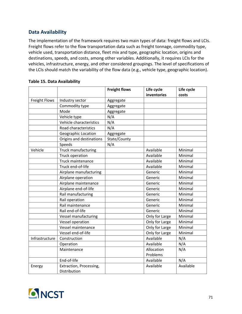
71

Data Availability

The implementation of the framework requires two main types of data: freight flows and LCIs. Freight flows refer to the flow transportation data such as freight tonnage, commodity type, vehicle used, transportation distance, fleet mix and type, geographic location, origins and destinations, speeds, and costs, among other variables. Additionally, it requires LCIs for the vehicles, infrastructure, energy, and other considered groupings. The level of specifications of the LCIs should match the variability of the flow data (e.g., vehicle type, geographic location). Table 15. Data Availability

Freight flows Life cycle inventories

Life cycle costs

Freight Flows Industry sector Aggregate

Commodity type Aggregate

Mode Aggregate Vehicle type N/A

Vehicle characteristics N/A

Road characteristics N/A

Geographic Location Aggregate Origins and destinations State/County

Speeds N/A

Vehicle Truck manufacturing Available Minimal Truck operation Available Minimal

Truck maintenance Available Minimal

Truck end-of-life Available Minimal Airplane manufacturing Generic Minimal

Airplane operation Generic Minimal

Airplane maintenance Generic Minimal

Airplane end-of-life Generic Minimal Rail manufacturing Generic Minimal

Rail operation Generic Minimal

Rail maintenance Generic Minimal Rail end-of-life Generic Minimal

Vessel manufacturing Only for Large Minimal

Vessel operation Only for Large Minimal

Vessel maintenance Only for Large Minimal Vessel end-of-life Only for Large Minimal

Infrastructure Construction Available N/A

Operation Available N/A Maintenance Allocation

Problems N/A

End-of-life Available N/A

Energy Extraction, Processing, Distribution

Available Available

72

Models Availability

Similar to the data limitations, the team identified a general lack of freight models that could generate the required data. In California, Caltrans hosts the California Statewide Travel Demand Model4. The model analyzes freight flows through the short and long distance commercial vehicle models. However, the embedded models estimate the productions, attractions, and tours based on industry sectors and other variables (e.g., commodity growth factors), and the outputs are zonal level aggregates. Other similar models at the Regional and MPO level may produce even more aggregate results. Consequently, there are no models capable of considering supply chains as the unit of analysis. Another limitation refers to the infrastructure assessment. In many cases, the agencies will not build new infrastructure, and most of the impacts result in the rehabilitation and maintenance of existing infrastructure. Currently, for instance, there are no models to allocate pavement impacts and costs resulting from different types of freight vehicles and flows. The literature also revealed the need to develop models to assess the impacts of different vehicles and fuel technologies. Considering the different modes, the data and models to estimate short haul and last-mile delivery traffic lack in comparison to the availability for long-haul movements.

4 http://www.dot.ca.gov/hq/tpp/offices/omsp/statewide_modeling/cstdm.html

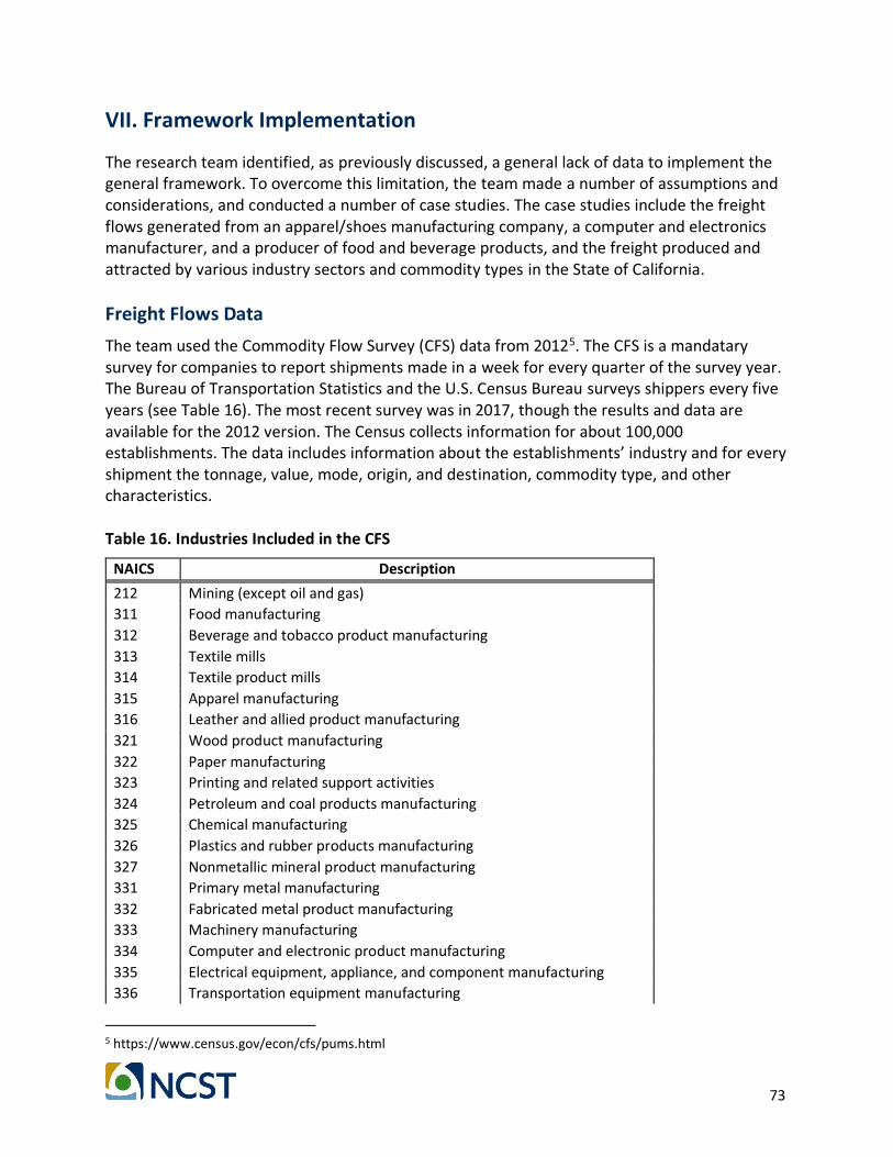
73

VII. Framework Implementation

The research team identified, as previously discussed, a general lack of data to implement the general framework. To overcome this limitation, the team made a number of assumptions and considerations, and conducted a number of case studies. The case studies include the freight flows generated from an apparel/shoes manufacturing company, a computer and electronics manufacturer, and a producer of food and beverage products, and the freight produced and attracted by various industry sectors and commodity types in the State of California.

Freight Flows Data

The team used the Commodity Flow Survey (CFS) data from 20125. The CFS is a mandatary survey for companies to report shipments made in a week for every quarter of the survey year. The Bureau of Transportation Statistics and the U.S. Census Bureau surveys shippers every five years (see Table 16). The most recent survey was in 2017, though the results and data are available for the 2012 version. The Census collects information for about 100,000 establishments. The data includes information about the establishments’ industry and for every shipment the tonnage, value, mode, origin, and destination, commodity type, and other characteristics. Table 16. Industries Included in the CFS

NAICS Description

212 Mining (except oil and gas)

311 Food manufacturing

312 Beverage and tobacco product manufacturing

313 Textile mills

314 Textile product mills

315 Apparel manufacturing

316 Leather and allied product manufacturing

321 Wood product manufacturing

322 Paper manufacturing

323 Printing and related support activities

324 Petroleum and coal products manufacturing

325 Chemical manufacturing

326 Plastics and rubber products manufacturing

327 Nonmetallic mineral product manufacturing

331 Primary metal manufacturing

332 Fabricated metal product manufacturing

333 Machinery manufacturing

334 Computer and electronic product manufacturing

335 Electrical equipment, appliance, and component manufacturing

336 Transportation equipment manufacturing

5 https://www.census.gov/econ/cfs/pums.html

74

NAICS Description

337 Furniture and related product manufacturing

339 Miscellaneous manufacturing

4231 Motor vehicle and parts merchant wholesalers

4232 Furniture and home furnishing merchant wholesalers

4233 Lumber and other construction materials merchant wholesalers

4234 Commercial equip. merchant wholesalers

4235 Metal and mineral (except petroleum) merchant wholesalers

4236 Electrical and electronic goods merchant wholesalers

4237 Hardware and plumbing merchant wholesalers

4238 Machinery, equipment, and supplies merchant wholesalers

4239 Miscellaneous durable goods merchant wholesalers

4241 Paper and paper product merchant wholesalers

4242 Drugs and druggists' sundries merchant wholesalers

4243 Apparel, piece goods, and notions merchant wholesalers

4244 Grocery and related product merchant wholesalers

4245 Farm product raw material merchant wholesalers

4246 Chemical and allied products merchant wholesalers

4247 Petroleum and petroleum products merchant wholesalers

4248 Beer, wine, and distilled alcoholic beverage merchant wholesalers

4249 Miscellaneous nondurable goods merchant wholesalers

4541 Electronic shopping and mail-order houses

45431 Direct selling establishments

4931 Warehousing and storage (includes 484)

5111 Newspaper, periodical, book, and directory publishers

551114 Corporate, subsidiary, and regional managing offices

Table 17 shows the Standard Classification of Transported Goods (SCTG) codes included in the CFS. Establishments in one specific industry may generate shipments of different types of commodities. Therefore, commodity-based analyses span multiple industries. Similarly, industry-based analyses span over multiple commodity types. Table 17. Commodities Transported

SCTG Description SCTG

Group

01 Animals and Fish (live) 01-05

02 Cereal Grains (includes seed)

03 Agricultural Products (excludes Animal Feed, Cereal Grains, and Forage Products)

04 Animal Feed, Eggs, Honey, and Other Products of Animal Origin

05 Meat, Poultry, Fish, Seafood, and Their Preparations

06 Milled Grain Products and Preparations, and Bakery Products 06-09

07 Other Prepared Foodstuffs, and Fats and Oils

75

SCTG Description SCTG

Group 08 Alcoholic Beverages and Denatured Alcohol

09 Tobacco Products

10 Monumental or Building Stone 10-14

11 Natural Sands

12 Gravel and Crushed Stone (excludes Dolomite and Slate)

13 Other Non-Metallic Minerals not elsewhere classified

14 Metallic Ores and Concentrates

15 Coal 15-19

16 Crude Petroleum

17 Gasoline, Aviation Turbine Fuel, and Ethanol (includes Kerosene, and Fuel Alcohols)

18 Fuel Oils (includes Diesel, Bunker C, and Biodiesel)

19 Other Coal and Petroleum Products, not elsewhere classified

20 Basic Chemicals 20-24

21 Pharmaceutical Products

22 Fertilizers

23 Other Chemical Products and Preparations

24 Plastics and Rubber

25 Logs and Other Wood in the Rough 25-30

26 Wood Products

27 Pulp, Newsprint, Paper, and Paperboard

28 Paper or Paperboard Articles

29 Printed Products

30 Textiles, Leather, and Articles of Textiles or Leather

31 Non-Metallic Mineral Products 31-34

32 Base Metal in Primary or Semi-Finished Forms and in Finished Basic Shapes

33 Articles of Base Metal

34 Machinery

35 Electronic and Other Electrical Equipment and Components, and Office Equipment

35-38

36 Motorized and Other Vehicles (includes parts)

37 Transportation Equipment, not elsewhere classified

38 Precision Instruments and Apparatus

39 Furniture, Mattresses and Mattress Supports, Lamps, Lighting Fittings 39-99

40 Miscellaneous Manufactured Products

41 Waste and Scrap (excludes of agriculture or food, see 041xx)

43 Mixed Freight

99 Missing Code

76

Table 18 shows the different transportation modes used to move freight. The distinction between for-hire trucks and private trucks is very important for the analyses and the goal of this project. This is because, without loss of generality, a carrier company (NAICS 484: Truck Transportation) provides the for-hire trucks, while the individual establishment operates the private trucks. Similarly, in the U.S. Class I railroad carriers transport the vast majority of the rail movements, and belong to the NAICS 482: Rail Transportation; carrier airlines (freight and passenger) are in the NAICS 481: Air Transportation; and NAICS 483 is Water Transportation. This distinction between the carrier and the shipper is an important consideration when designing transportation policies. As mentioned before, the carrier companies are the conduit between other economic agents, which are ultimately responsible for the cargo movements and the logistics decisions. However, most of the regulations only consider the vehicles and carriers’ operations. For many decades, the CFS only published aggregated results at the County, State, or MSA levels of the data (tabulations). In 2012, the Census Bureau published the first generation of the 2012 CFS Public Use Microdata (PUM). This experimental data contains information for approximately 4.5 million shipments from the 2012 CFS. The Bureau used a number of statistical tools and methods to create the synthetic shipment data to protect the confidentiality of individual business information. The research team developed a spreadsheet-based tool to manipulate the data. The tool can produce tabulations of shipment tonnage, ton-miles, value per industry sector, commodity type, mode or any other of the variables contained in the CFS-PUM. For the analyses, the team uses the CFS-PUM as the freight flow data. Table 18. Transportation Modes in the CFS

04 For-hire truck 03 Truck 02

05 Private truck

06 Rail

08 Inland Water 07 Water

09 Great Lakes

10 Deep Sea

101 Multiple Waterways

11 Air (incl truck & air)

12 Pipeline

19 Other mode

14 Parcel, USPS, or courier 13

15 Truck and rail 20

16 Truck and water

17 Rail and water

18 Other multiple mode

Most Detailed Mode Codes

Single mode

Multiple

mode

1st Collapsing 2nd Collapsing

Non-

parcel

multiple

mode

77

CFS-PUM Freight Flows in California

The team estimated the ton-miles for different industries and commodities originating from or destined to California in 2012 using the different modes. Figure 15 shows the magnitude for the various industries. There is no symmetry in the freight flows, and it is evident that for the high-volume industries, the majority of the cargo shipped out uses rail, while most of the cargo destined to California (from U.S. establishments) arrives by truck. Looking at the 3-digit level NAICS codes, the State generates and attracts a large percentage of NAICS 311: food-manufacturing products. In terms of attraction, other significant industries include NAICS 4231: Motor vehicle and parts merchant wholesalers, NAICS 312: Beverage and tobacco product manufacturing; NAICS 4244 Grocery and related product merchant wholesalers; and NAICS 551114: Corporate, subsidiary, and regional managing offices. For outbound shipments, NAICS 311, NAICS 325: Chemical manufacturing and NAICS 4245: Farm product raw material merchant wholesalers represent the largest shares. Figure 16 compares the mode shares for the different industries. It is clear that for-hire trucks dominate the freight movements, with rail being significant for outbound cargo. For some of the industries, private trucking is important, though the industries tend to generate low ton-miles. For example, NAICS 45431: Direct selling establishments transport most of the cargo using private trucks. Some of these industries tend to have destinations at shorter distances. This is important aggregate information; however, no additional information translates the general modes to specific vehicles types or classes. California is an important consumption destination; Figure 17 shows the inbound and outbound ton-miles for different commodity groups. SCTG 7: Other prepared foodstuffs, and fats and oil represent the largest percentage of the inbound cargo. This is also an important commodity group for outbound shipments, as well as SCTG 2: Cereal grains (including seeds). Consistent with the industry-based picture from Figure 15, there is a higher share of rail outbound shipments. Figure 18 shows the mode shares per commodity. Almost all SCTG 2 shipments use rail, and all coal transport is by rail. In addition, about half of agricultural products (SCTG 3 and SCTG 4) shipments use rail. However, the majority of inbound and outbound shipments use truck (with for-hire trucks dominating). There are a number of commodity groups that use private fleets, and these tend to be commodities requiring specialized vehicles such as SCTG 10: Monumental or building stone, SCTG 11: Natural sands, SCTG 12: Gravel and crushed stone, SCTG 18: Fuel oils, and SCTG 25: Logs and other wood in the rough. These flows evidence different types of freight patterns resulting from the type of commodity. This is not clearly identified at the industry group level.

78

Figure 15. Ton-miles Originated from (Out) and Destined to (In) California in 2012 per Industry Sector per Mode of Transport

-

5,000

10,000

15,000

20,000

25,000

30,000

212

311

312

313

314

315

316

321

322

323

324

325

326

327

331

332

333

334

335

336

337

339

423

1

423

2

423

3

423

4

423

5

423

6

423

7

423

8

423

9

424

1

424

2

424

3

424

4

424

5

424

6

424

7

424

8

424

9

454

1

45

43

1

493

1

511

1

551

114

Mill

ion

sInbound

Air Rail Parcel, USPS, or courier Private truck For-hire truck Truck multimodal Water (Deep Sea, Inland waterways)

-

5,000

10,000

15,000

20,000

25,000

30,000

35,000

40,000

212

311

312

313

314

315

316

321

322

323

324

325

326

327

331

332

333

334

335

336

337

339

423

1

423

2

423

3

423

4

423

5

423

6

423

7

423

8

423

9

424

1

424

2

424

3

424

4

424

5

424

6

424

7

424

8

424

9

454

1

454

31

493

1

511

1

55

1,11

4

Mill

ion

s

Outbound

Air Rail Parcel, USPS, or courier Private truck For-hire truck Truck multimodal Water (Deep Sea, Inland waterways)

79

Figure 16. Comparative Mode Share for Ton-miles Originated from (Out) and Destined to (In) California in 2012 per Industry Sector

0%

20%

40%

60%

80%

100%21

2

311

312

313

314

315

316

321

322

323

324

325

326

327

331

332

333

334

335

336

337

339

423

1

423

2

423

3

423

4

423

5

423

6

423

7

423

8

423

9

424

1

424

2

424

3

424

4

424

5

424

6

424

7

424

8

424

9

454

1

454

31

493

1

511

1

55

1,11

4

Inbound

Air Rail Parcel, USPS, or courier Private truck For-hire truck Truck multimodal Water (Deep Sea, Inland waterways)

0%

20%

40%

60%

80%

100%

212

311

312

313

314

315

316

321

322

323

324

325

326

327

331

332

333

334

335

336

337

339

423

1

423

2

423

3

423

4

423

5

423

6

423

7

423

8

423

9

424

1

424

2

424

3

424

4

424

5

424

6

424

7

424

8

424

9

454

1

454

31

493

1

511

1

55

1,11

4

Outbound

Air Rail Parcel, USPS, or courier Private truck For-hire truck Truck multimodal Water (Deep Sea, Inland waterways)

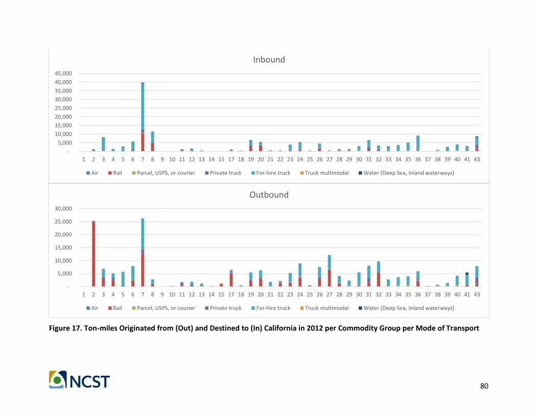
80

Figure 17. Ton-miles Originated from (Out) and Destined to (In) California in 2012 per Commodity Group per Mode of Transport

-

5,000

10,000

15,000

20,000

25,000

30,000

35,000

40,000

45,000

1 2 3 4 5 6 7 8 9 10 11 12 13 14 15 17 18 19 20 21 22 23 24 25 26 27 28 29 30 31 32 33 34 35 36 37 38 39 40 41 43

Inbound

Air Rail Parcel, USPS, or courier Private truck For-hire truck Truck multimodal Water (Deep Sea, Inland waterways)

-

5,000

10,000

15,000

20,000

25,000

30,000

1 2 3 4 5 6 7 8 9 10 11 12 13 14 15 17 18 19 20 21 22 23 24 25 26 27 28 29 30 31 32 33 34 35 36 37 38 39 40 41 43

Outbound

Air Rail Parcel, USPS, or courier Private truck For-hire truck Truck multimodal Water (Deep Sea, Inland waterways)

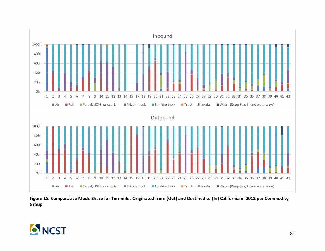
81

Figure 18. Comparative Mode Share for Ton-miles Originated from (Out) and Destined to (In) California in 2012 per Commodity Group

0%

20%

40%

60%

80%

100%

1 2 3 4 5 6 7 8 9 10 11 12 13 14 15 17 18 19 20 21 22 23 24 25 26 27 28 29 30 31 32 33 34 35 36 37 38 39 40 41 43

Inbound

Air Rail Parcel, USPS, or courier Private truck For-hire truck Truck multimodal Water (Deep Sea, Inland waterways)

0%

20%

40%

60%

80%

100%

1 2 3 4 5 6 7 8 9 10 11 12 13 14 15 17 18 19 20 21 22 23 24 25 26 27 28 29 30 31 32 33 34 35 36 37 38 39 40 41 43

Outbound

Air Rail Parcel, USPS, or courier Private truck For-hire truck Truck multimodal Water (Deep Sea, Inland waterways)

82

Life Cycle Inventory Data

For the LCI data, the team found various sources. For example, EMFAC provides life cycle data for various vehicle and technology types, and GREET assess the life cycle of energy sources. However, the available disaggregate data did not include all processes (e.g., production/construction, operation, maintenance) for the vehicles, and the infrastructure in particular. Considering the other databases (see Annex A), the team used Gabi to identify inventories for the implementation. Most of the available inventories in Gabi are from Ecoinvent 3.0 and may include global, regional or country data for specific or aggregate processes. The team selected U.S. or global inventories and sought inventories for the transport of goods related to the various modes under consideration. Table 19 shows examples of aggregate transport processes. From the available inventories, the team selected: Rail:

▪ Market for transport, freight train

Water:

▪ Transport, freight, sea, transoceanic ship

Air:

▪ Market for transport, freight, aircraft

Truck:

▪ Transport, freight, lorry with refrigeration machine, 3.5-7.5 ton, EURO3, carbon dioxide,

liquid refrigeration

▪ Market for transport, freight, lorry 3.5-7.5 metric ton, EURO3

▪ Transport, freight, lorry with refrigeration machine, 3.5-7.5 ton, EURO4, carbon dioxide,

liquid refrigeration

▪ Market for transport, freight, lorry 3.5-7.5 metric ton, EURO4

▪ Transport, freight, lorry with refrigeration machine, 3.5-7.5 ton, EURO5, carbon dioxide,

liquid refrigeration

▪ Market for transport, freight, lorry 3.5-7.5 metric ton, EURO5

▪ Transport, freight, lorry with refrigeration machine, 7.5-16 ton, EURO3, carbon dioxide,

liquid refrigeration

▪ Market for transport, freight, lorry 7.5-16 metric ton, EURO3

▪ Transport, freight, lorry with refrigeration machine, 7.5-16 ton, EURO4, carbon dioxide,

liquid refrigeration

▪ Market for transport, freight, lorry 7.5-16 metric ton, EURO4

▪ Transport, freight, lorry with refrigeration machine, 7.5-16 ton, EURO5, carbon dioxide,

liquid refrigeration

▪ Market for transport, freight, lorry 7.5-16 metric ton, EURO5

83

▪ Market for transport, freight, lorry 16-32 metric ton, EURO3

▪ Market for transport, freight, lorry 16-32 metric ton, EURO4

▪ Market for transport, freight, lorry 16-32 metric ton, EURO5

The team found that the transoceanic ship inventory does not completely reflect the flows for this process. As previously discussed, the existing flow data (ton-miles) does not identify the type of vehicle (fleet mix) used. Therefore, using these inventories, team developed generic LCIs assuming the fleet composition in the 2012 EMFAC vehicle population data as the mix transporting the flows in the CFS-PUM.

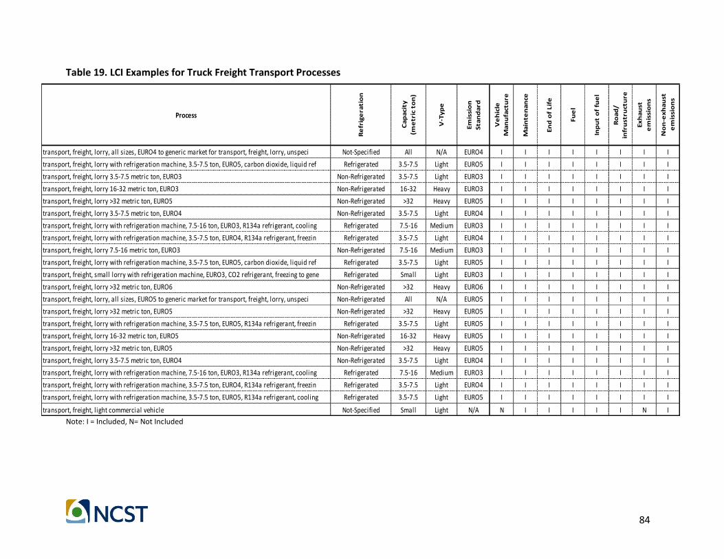
84

Table 19. LCI Examples for Truck Freight Transport Processes

Process

Re

frig

era

tio

n

Ca

pa

city

(me

tric

to

n)

V-T

yp

e

Em

issi

on

Sta

nd

ard

Ve

hic

le

Ma

nu

fact

ure

Ma

inte

na

nce

En

d o

f L

ife

Fu

el

Inp

ut

of

fue

l

Ro

ad

/

infr

ust

ruct

ure

Ex

ha

ust

em

issi

on

s

No

n-e

xh

au

st

em

issi

on

s

transport, freight, lorry, all sizes, EURO4 to generic market for transport, freight, lorry, unspeci Not-Specified All N/A EURO4 I I I I I I I I

transport, freight, lorry with refrigeration machine, 3.5-7.5 ton, EURO5, carbon dioxide, l iquid ref Refrigerated 3.5-7.5 Light EURO5 I I I I I I I I

transport, freight, lorry 3.5-7.5 metric ton, EURO3 Non-Refrigerated 3.5-7.5 Light EURO3 I I I I I I I I

transport, freight, lorry 16-32 metric ton, EURO3 Non-Refrigerated 16-32 Heavy EURO3 I I I I I I I I

transport, freight, lorry >32 metric ton, EURO5 Non-Refrigerated >32 Heavy EURO5 I I I I I I I I

transport, freight, lorry 3.5-7.5 metric ton, EURO4 Non-Refrigerated 3.5-7.5 Light EURO4 I I I I I I I I

transport, freight, lorry with refrigeration machine, 7.5-16 ton, EURO3, R134a refrigerant, cooling Refrigerated 7.5-16 Medium EURO3 I I I I I I I I

transport, freight, lorry with refrigeration machine, 3.5-7.5 ton, EURO4, R134a refrigerant, freezin Refrigerated 3.5-7.5 Light EURO4 I I I I I I I I

transport, freight, lorry 7.5-16 metric ton, EURO3 Non-Refrigerated 7.5-16 Medium EURO3 I I I I I I I I

transport, freight, lorry with refrigeration machine, 3.5-7.5 ton, EURO5, carbon dioxide, l iquid ref Refrigerated 3.5-7.5 Light EURO5 I I I I I I I I

transport, freight, small lorry with refrigeration machine, EURO3, CO2 refrigerant, freezing to gene Refrigerated Small Light EURO3 I I I I I I I I

transport, freight, lorry >32 metric ton, EURO6 Non-Refrigerated >32 Heavy EURO6 I I I I I I I I

transport, freight, lorry, all sizes, EURO5 to generic market for transport, freight, lorry, unspeci Non-Refrigerated All N/A EURO5 I I I I I I I I

transport, freight, lorry >32 metric ton, EURO5 Non-Refrigerated >32 Heavy EURO5 I I I I I I I I

transport, freight, lorry with refrigeration machine, 3.5-7.5 ton, EURO5, R134a refrigerant, freezin Refrigerated 3.5-7.5 Light EURO5 I I I I I I I I

transport, freight, lorry 16-32 metric ton, EURO5 Non-Refrigerated 16-32 Heavy EURO5 I I I I I I I I

transport, freight, lorry >32 metric ton, EURO5 Non-Refrigerated >32 Heavy EURO5 I I I I I I I I

transport, freight, lorry 3.5-7.5 metric ton, EURO4 Non-Refrigerated 3.5-7.5 Light EURO4 I I I I I I I I

transport, freight, lorry with refrigeration machine, 7.5-16 ton, EURO3, R134a refrigerant, cooling Refrigerated 7.5-16 Medium EURO3 I I I I I I I I

transport, freight, lorry with refrigeration machine, 3.5-7.5 ton, EURO4, R134a refrigerant, freezin Refrigerated 3.5-7.5 Light EURO4 I I I I I I I I

transport, freight, lorry with refrigeration machine, 3.5-7.5 ton, EURO5, R134a refrigerant, cooling Refrigerated 3.5-7.5 Light EURO5 I I I I I I I I

transport, freight, l ight commercial vehicle Not-Specified Small Light N/A N I I I I I N I Note: I = Included, N= Not Included

85

EMFAC Vehicle Population

Considering Gabi presents the LCIs for the European context, the team created a crosswalk for the vehicle categories and considered light heavy duty, medium-heavy-duty, and heavy-heavy-duty vehicles from EMFAC. These are a combination of Class 3 – Class 8 FHWA classes. Moreover, the team used the vehicle model and class to assume EURO standard classifications for the EMFAC vehicle population. Table 20 summarizes the vehicle population in California from the EMFAC 2012, and Figure 19 shows the shares of EURO standards for these vehicles. Table 20. EMFAC 2012 Vehicle Population

Before Euro

Euro 0 Euro I Euro II Euro III Euro IV Euro V Grand Total

Light 36,524

12,550 23,151 142,653 88,952 57,461 361,290

Medium 49,086

15,422 31,201 115,905 96,740 77,737 386,091

Heavy 23,487 12,816 11,891 20,460 51,916 39,590 49,671 209,831 Grand Total

109,097 12,816 39,862 74,813 310,473 225,282 184,869 957,212

Figure 19. EURO Shares for Different Vehicles Types

Considering the availability of process inventories for truck transport for EUROs III to V, the team estimated the adjusted shares for the vehicle population using these vehicles as the entire population. Table 21 shows the adjusted factors.

0% 20% 40% 60% 80% 100%

Light

Medium

Heavy

Before_Euro Euro 0 Euro I Euro II Euro III Euro IV Euro V

86

Table 21. Adjusted EURO Standard Fleet Composition

Euro III Euro IV Euro V

Light 49.35% 30.77% 19.88%

Medium 39.91% 33.31% 26.77%

Heavy 36.77% 28.04% 35.18%

Grand Total 43.08% 31.26% 25.65%

With these adjusted factors, the team generated the following generic vehicle type LCIs to use in the analyses:

▪ Transport, freight, lorry, all

▪ Transport, freight, lorry, non_refrigerated

▪ Transport, freight, lorry, refrigerated

▪ Transport, freight, small lorry, all

▪ Transport, freight, small lorry, refrigerated

▪ Transport, freight, small lorry, non_refrigerated

▪ Transport, freight, medium lorry, all

▪ Transport, freight, medium lorry, non_refrigerated

▪ Transport, freight, medium lorry, refrigerated

▪ Transport, freight, large lorry, all

▪ Transport, freight, large lorry, non_refrigerated

Impact Categories

The next step required defining the impact categories. The team selected the widely used US. EPA Tool for the Reduction and Assessment of Chemical and Other Environmental Impacts (TRACI). Table 22 describes the various TRACI impacts.

87

Table 22. TRACI Impact Categories

Impact Description

Global warming potential (GWP)

Mass of carbon dioxide (CO2) equivalent emissions to air with the potential to contribute to global warming, combining emissions of CO2, N2O, CH4, and other potent GHG emissions based on their relative contribution to radiative forcing on a 100-year time horizon

Acidification potential Mass of emissions that contribute to acidic pollution expressed as equivalent hydrogen ions (H+) from nitrogen and sulfur emissions to soil and water

Ozone depletion potential Mass of substances released to air that could deplete stratospheric ozone reported in chlorofluorocarbon-11 equivalents

Eutrophication potential Mass of emissions to air and water that can enrich freshwater and coastal water bodies with nitrates or phosphates represented in nitrogen equivalents. These pollutants can accelerate biological productivity (growth of algae and weeds) and deplete oxygen in aquatic ecosystems

Photochemical smog formation potential

Mass of air emissions of NOx, VOCs, and other ground level ozone forming chemicals reported in units of ozone equivalence. TRACI uses the maximum incremental reactivity method to estimate the likely tropospheric ozone smog formation potential from VOCs, which have several chemical fate pathways

Resource depletion Mass of fossil fuel, volume of water, or area land use; context is critical to this indicator as different places and resources have different availabilities

Human health - particulate Mass of air pollution emissions including particulate matter consisting of inhalable coarse particles between 2.5 and 10 microns (PM10) & fine particles less than or equal to 2.5 microns (PM2.5) and their precursors

Human health - cancer comparative toxicity unit (CTUcancer), human health non-cancer comparative toxicity unit (CTUnon-cancer), and Ecotoxicity comparative toxicity unit (CTUeco)

Metrics that represent the emissions of known carcinogens and toxics to urban air, nonurban air, freshwater, seawater, natural soil, and agricultural soil based on a chemical fate model. Human health cancer aims to provide information about emissions known to cause human cancer. Human health non-cancer represents contributions to other kinds of toxicity. Ecotoxicity estimates freshwater or marine toxicity or damage.

Source: Adapted from (Bare, 2011)

The team used TRACI and the LCIs to estimate the various impacts for the different modes (see Table 23). These impacts are per ton-kilometer.

88

Table 23. TRACI Impacts for the Different Modes

Rail Air Transoceanic Ship

Ecotoxicity CTUeco/tkm 1.6508E-01 3.4619E-01 6.7480E-11

HumantoxCAN CTUcancer/tkm 5.1802E-09 5.6156E-09 0.0000E+00

HumantoxNC CTUnoncancer/tkm 8.4591E-09 2.7572E-08 0.0000E+00

GWP kg CO2 eq/tkm 5.8033E-02 1.1179E+00 2.6279E-10

Resources 0.0000E+00 0.0000E+00 0.0000E+00

Humanpartic PM2.5eq/tkm 8.1106E-05 2.8981E-04 0.0000E+00

ODP kg CFC-11 eq/tkm 1.1368E-08 2.7340E-07 2.1599E-13

Smog kg O3 eq/tkm 1.6514E-02 1.1934E-01 3.7908E-13

Accidification kg SO2 eq/tkm 5.7409E-04 4.8835E-03 0.0000E+00

Eutrophication kg N eq/tkm 1.1649E-04 7.7583E-04 0.0000E+00

All Small Medium Large

Ecotoxicity CTUeco/tkm 1.1471E+00 1.9317E+00 6.7691E-01 4.5925E-01

HumantoxCAN CTUcancer/tkm 1.3866E-08 2.4175E-08 8.0006E-09 4.3660E-09

HumantoxNC CTUnoncancer/tkm 1.4494E-07 2.1448E-07 1.0192E-07 8.2363E-08

GWP kg CO2 eq/tkm 3.5490E-01 5.6604E-01 2.3634E-01 1.5053E-01

Resources 0.0000E+00 0.0000E+00 0.0000E+00 0.0000E+00

Humanpartic PM2.5eq/tkm 3.6035E-04 5.5823E-04 2.4377E-04 1.7725E-04

ODP kg CFC-11 eq/tkm 8.2394E-08 1.2940E-07 5.5819E-08 3.6934E-08

Smog kg O3 eq/tkm 4.1342E-02 6.5559E-02 2.7562E-02 1.8871E-02

Accidification kg SO2 eq/tkm 1.7352E-03 2.7815E-03 1.1419E-03 7.5506E-04

Eutrophication kg N eq/tkm 4.6276E-04 7.7116E-04 2.8889E-04 1.7213E-04

All Small Medium Large

Ecotoxicity CTUeco/tkm 1.3172E+00 2.1890E+00 7.5155E-01 4.5925E-01

HumantoxCAN CTUcancer/tkm 1.3404E-08 2.2574E-08 7.4787E-09 4.3660E-09

HumantoxNC CTUnoncancer/tkm 1.5093E-07 2.2097E-07 1.0366E-07 8.2363E-08

GWP kg CO2 eq/tkm 3.3354E-01 5.1596E-01 2.1551E-01 1.5053E-01

Resources 0.0000E+00 0.0000E+00 0.0000E+00 0.0000E+00

Humanpartic PM2.5eq/tkm 3.4991E-04 5.2893E-04 2.3255E-04 1.7725E-04

ODP kg CFC-11 eq/tkm 7.7976E-08 1.1895E-07 5.1336E-08 3.6934E-08

Smog kg O3 eq/tkm 3.8446E-02 5.9933E-02 2.5220E-02 1.8871E-02

Accidification kg SO2 eq/tkm 1.6187E-03 2.5374E-03 1.0427E-03 7.5506E-04

Eutrophication kg N eq/tkm 4.2933E-04 6.9207E-04 2.6032E-04 1.7213E-04

All Small Medium Large

Ecotoxicity CTUeco/tkm 9.4148E-01 1.6743E+00 6.0226E-01

HumantoxCAN CTUcancer/tkm 1.4219E-08 2.5775E-08 8.5224E-09

HumantoxNC CTUnoncancer/tkm 1.2623E-07 2.0800E-07 1.0018E-07

GWP kg CO2 eq/tkm 3.5930E-01 6.1612E-01 2.5718E-01

Resources 0.0000E+00 0.0000E+00 0.0000E+00

Humanpartic PM2.5eq/tkm 3.4493E-04 5.8753E-04 2.5499E-04

ODP kg CFC-11 eq/tkm 8.2253E-08 1.3984E-07 6.0302E-08

Smog kg O3 eq/tkm 4.0961E-02 7.1185E-02 2.9904E-02

Accidification kg SO2 eq/tkm 1.7392E-03 3.0255E-03 1.2410E-03

Eutrophication kg N eq/tkm 4.8117E-04 8.5025E-04 3.1747E-04

TRACI Category

transport, freight, lorry, all

transport, freight, lorry, non_refrigerated

transport, freight, lorry, refrigerated

market for transport, freight/ transport, freight

TRACI Category

TRACI Category

TRACI Category

89

Figure 20, Figure 21, and Figure 22 provide a visual comparison of the various modes/vehicles. The results show great variability, with refrigeration becoming an important contributing factor to, in general, larger impacts. However, it is important to recognize that these estimates are for generic vehicles using averages of the vehicle population and other assumptions. As discussed in this document, uncertainty and data quality are important aspects of LCA analyses. The variability in these inventories is an example.

Figure 20. Ecotoxicity and Human Toxicity per Ton-Km

0

0.5

1

1.5

2

2.5

Ecotoxicity CTUeco/tkm

0

5E-09

1E-08

1.5E-08

2E-08

2.5E-08

3E-08

HumantoxCAN CTUcancer/tkm

0

5E-08

0.0000001

1.5E-07

0.0000002

2.5E-07

HumantoxNC CTUnoncancer/tkm

90

Figure 21. GWP, Human Particles, and Ozone Depletion Potential per Ton-Km

0

0.5

1

1.5

GWP kg CO2eq/tkm

0

0.0002

0.0004

0.0006

0.0008

Humanpartic PM2.5eq/tkm

0

5E-08

0.0000001

1.5E-07

0.0000002

2.5E-07

0.0000003

Ozone Depletion Potential kg CFC-11eq/tkm

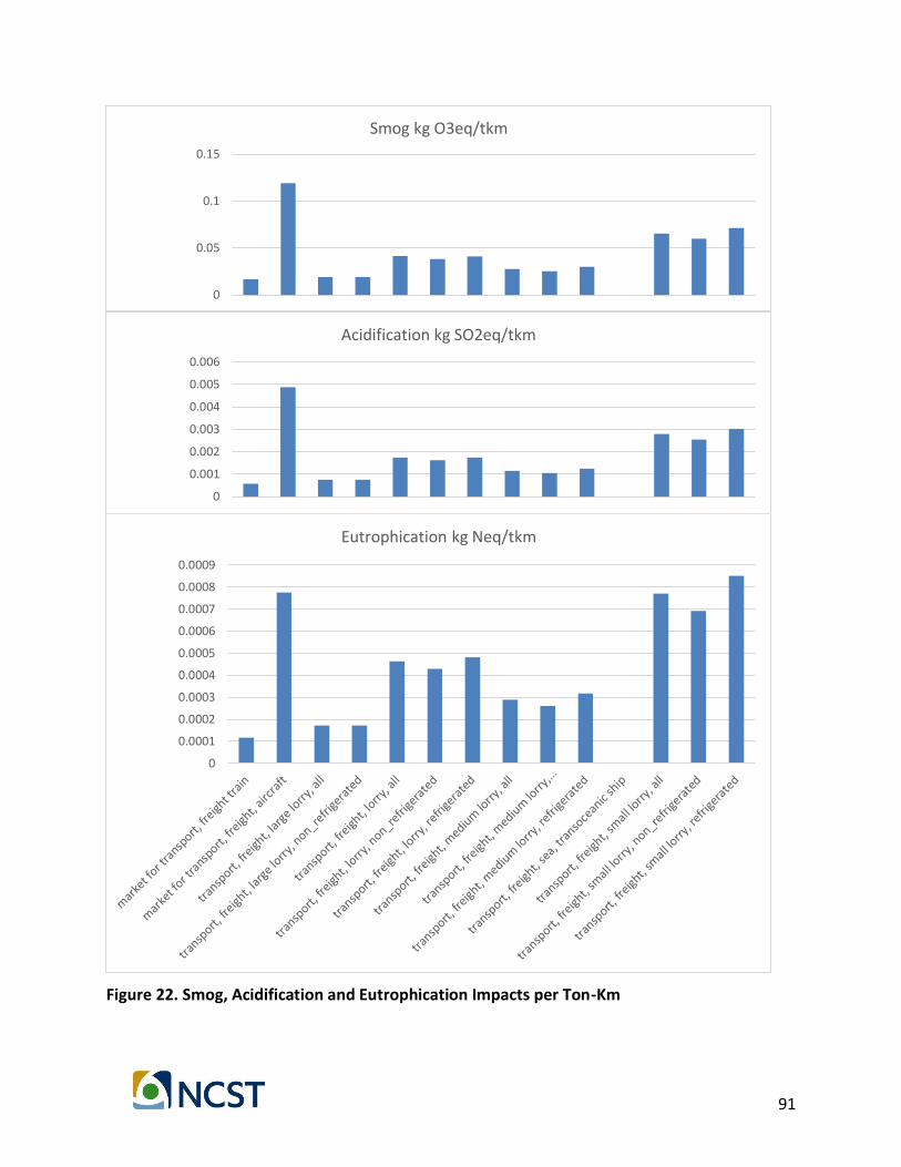
91

Figure 22. Smog, Acidification and Eutrophication Impacts per Ton-Km

0

0.05

0.1

0.15

Smog kg O3eq/tkm

0

0.001

0.002

0.003

0.004

0.005

0.006

Acidification kg SO2eq/tkm

0

0.0001

0.0002

0.0003

0.0004

0.0005

0.0006

0.0007

0.0008

0.0009

Eutrophication kg Neq/tkm

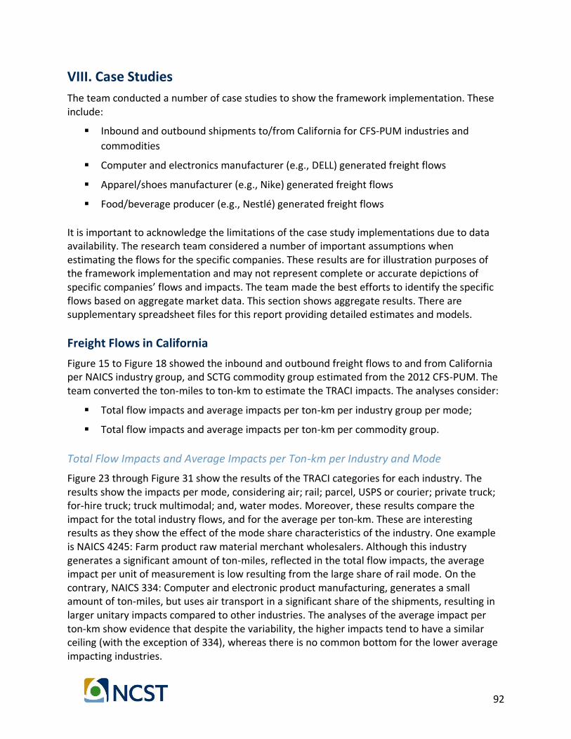
92

VIII. Case Studies

The team conducted a number of case studies to show the framework implementation. These include:

▪ Inbound and outbound shipments to/from California for CFS-PUM industries and

commodities

▪ Computer and electronics manufacturer (e.g., DELL) generated freight flows

▪ Apparel/shoes manufacturer (e.g., Nike) generated freight flows

▪ Food/beverage producer (e.g., Nestlé) generated freight flows

It is important to acknowledge the limitations of the case study implementations due to data availability. The research team considered a number of important assumptions when estimating the flows for the specific companies. These results are for illustration purposes of the framework implementation and may not represent complete or accurate depictions of specific companies’ flows and impacts. The team made the best efforts to identify the specific flows based on aggregate market data. This section shows aggregate results. There are supplementary spreadsheet files for this report providing detailed estimates and models.

Freight Flows in California

Figure 15 to Figure 18 showed the inbound and outbound freight flows to and from California per NAICS industry group, and SCTG commodity group estimated from the 2012 CFS-PUM. The team converted the ton-miles to ton-km to estimate the TRACI impacts. The analyses consider:

▪ Total flow impacts and average impacts per ton-km per industry group per mode;

▪ Total flow impacts and average impacts per ton-km per commodity group.

Total Flow Impacts and Average Impacts per Ton-km per Industry and Mode

Figure 23 through Figure 31 show the results of the TRACI categories for each industry. The results show the impacts per mode, considering air; rail; parcel, USPS or courier; private truck; for-hire truck; truck multimodal; and, water modes. Moreover, these results compare the impact for the total industry flows, and for the average per ton-km. These are interesting results as they show the effect of the mode share characteristics of the industry. One example is NAICS 4245: Farm product raw material merchant wholesalers. Although this industry generates a significant amount of ton-miles, reflected in the total flow impacts, the average impact per unit of measurement is low resulting from the large share of rail mode. On the contrary, NAICS 334: Computer and electronic product manufacturing, generates a small amount of ton-miles, but uses air transport in a significant share of the shipments, resulting in larger unitary impacts compared to other industries. The analyses of the average impact per ton-km show evidence that despite the variability, the higher impacts tend to have a similar ceiling (with the exception of 334), whereas there is no common bottom for the lower average impacting industries.

93

Figure 32 shows the TRACI impacts for all (only including the CFS-PUM industries) freight flows in California. As expected, the majority of the impacts come from the ton-km using for-hire trucks because this mode transports most of the cargo. Rail is the second popular mode, and the impacts reflect this relationship and the lower per ton-km TRACI impacts. The results show that, for instance, the GWP impacts are about 150 million ton CO2eq for the yearly flows, with almost 120 million of those generated by trucks.

94

Figure 23. Ecotoxicity Impacts from All California Flows (top) and Average per Ton-km (bottom) for each Industry Category

0

0.2

0.4

0.6

0.8

1

1.2

1.4

All

212

311

312

313

314

315

316

321

322

323

324

325

326

327

331

332

333

334

335

336

337

339

423

1

423

2

423

3

423

4

423

5

423

6

423

7

423

8

423

9

424

1

424

2

424

3

424

4

424

5

424

6

424

7

424

8

424

9

454

1

454

31

493

1

511

1

551

114

Ecotoxicity CTUeco/tkm

0

10000

20000

30000

40000

50000

60000

70000

80000

90000

212

311

312

313

314

315

316

321

322

323

324

325

326

327

331

332

333

334

335

336

337

339

423

1

423

2

423

3

423

4

423

5

423

6

423

7

423

8

423

9

424

1

424

2

424

3

424

4

424

5

424

6

424

7

424

8

424

9

454

1

454

31

493

1

511

1

551

114

Mill

ion

sEcotoxicity - All Flows

Air Rail Parcel, USPS, or courier Private truck For-hire truck Truck multimodal Water (Deep Sea, Inland waterways)

95

Figure 24. Human Health Cancer Impacts from All California Flows (top) and Average per Ton-km (bottom) for each Industry Category

0

2E-09

4E-09

6E-09

8E-09

1E-08

1.2E-08

1.4E-08

1.6E-08

All

212

311

312

313

314

315

316

321

322

323

324

325

326

327

331

332

333

334

335

336

337

339

423

1

423

2

423

3

423

4

423

5

423

6

423

7

423

8

423

9

424

1

424

2

424

3

424

4

424

5

424

6

424

7

424

8

424

9

454

1

454

31

493

1

511

1

551

114

HumantoxCAN - CTUcancer/tkm

0

200

400

600

800

1,000

1,20021

2

311

312

313

314

315

316

321

322

323

324

325

326

327

331

332

333

334

335

336

337

339

423

1

423

2

423

3

423

4

423

5

423

6

423

7

423

8

423

9

424

1

424

2

424

3

424

4

424

5

424

6

424

7

424

8

424

9

454

1

454

31

493

1

511

1

551

114

HumantoxCAN - All Flows

Air Rail Parcel, USPS, or courier Private truck For-hire truck Truck multimodal Water (Deep Sea, Inland waterways)

96

Figure 25. Human Health Non-Cancer Impacts from All California Flows (top) and Average per Ton-km (bottom) for each Industry Category

0

2,000

4,000

6,000

8,000

10,000

12,000

21

2

31

1

31

2

31

3

31

4

31

5

31

6

32

1

32

2

32

3

32

4

32

5

32

6

32

7

33

1

33

2

33

3

33

4

33

5

33

6

33

7

33

9

42

31

42

32

42

33

42

34

42

35

42

36

42

37

42

38

42

39

42

41

42

42

42

43

42

44

42

45

42

46

42

47

42

48

42

49

45

41

45

43

1

49

31

51

11

55

11

14

HumantoxNC - All Flows

Air Rail Parcel, USPS, or courier Private truck For-hire truck Truck multimodal Water (Deep Sea, Inland waterways)

0

2E-08

4E-08

6E-08

8E-08

0.0000001

1.2E-07

1.4E-07

1.6E-07

All

212

311

312

313

314

315

316

321

322

323

324

325

326

327

331

332

333

334

335

336

337

339

423

1

423

2

423

3

423

4

423

5

423

6

423

7

423

8

423

9

424

1

424

2

424

3

424

4

424

5

424

6

424

7

424

8

424

9

454

1

454

31

493

1

511

1

551

114

HumantoxNC - CTUnoncanter/tkm

0

2E-08

4E-08

6E-08

8E-08

0.0000001

1.2E-07

1.4E-07

1.6E-07

All

212

311

312

313

314

315

316

321

322

323

324

325

326

327

331

332

333

334

335

336

337

339

423

1

423

2

423

3

423

4

423

5

423

6

423

7

423

8

423

9

424

1

424

2

424

3

424

4

424

5

424

6

424

7

424

8

424

9

454

1

454

31

493

1

511

1

551

114

HumantoxNC - CTUnoncanter/tkm

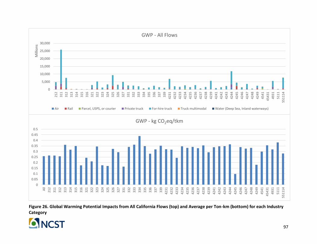
97

Figure 26. Global Warming Potential Impacts from All California Flows (top) and Average per Ton-km (bottom) for each Industry Category

0

5,000

10,000

15,000

20,000

25,000

30,000

212

311

312

313

314

315

316

321

322

323

324

325

326

327

331

332

333

334

335

336

337

339

423

1

423

2

423

3

423

4

423

5

423

6

423

7

423

8

423

9

424

1

424

2

424

3

424

4

424

5

424

6

424

7

424

8

424

9

454

1

454

31

493

1

511

1

551

114

Mill

ion

sGWP - All Flows

Air Rail Parcel, USPS, or courier Private truck For-hire truck Truck multimodal Water (Deep Sea, Inland waterways)

0

0.05

0.1

0.15

0.2

0.25

0.3

0.35

0.4

0.45

0.5

All

212

311

312

313

314

315

316

321

322

323

324

325

326

327

331

332

333

334

335

336

337

339

423

1

423

2

423

3

423

4

423

5

423

6

423

7

423

8

423

9

424

1

424

2

424

3

424

4

424

5

424

6

424

7

424

8

424

9

454

1

454

31

493

1

511

1

551

114

GWP - kg CO2eq/tkm

98

Figure 27. Human Health Particulate Impacts from All California Flows (top) and Average per Ton-km (bottom) for each Industry Category

0

0.00005

0.0001

0.00015

0.0002

0.00025

0.0003

0.00035

0.0004

All

212

311

312

313

314

315

316

321

322

323

324

325

326

327

331

332

333

334

335

336

337

339

423

1

423

2

423

3

423

4

423

5

423

6

423

7

423

8

423

9

424

1

424

2

424

3

424

4

424

5

424

6

424

7

424

8

424

9

454

1

454

31

493

1

511

1

551

114

Humanpartic - PM2.5eq/tkm

0

5

10

15

20

25

30

212

311

312

313

314

315

316

321

322

323

324

325

326

327

331

332

333

334

335

336

337

339

423

1

423

2

423

3

423

4

423

5

423

6

423

7

423

8

423

9

424

1

424

2

424

3

424

4

424

5

424

6

424

7

424

8

424

9

454

1

454

31

493

1

511

1

551

114

Mill

ion

sHumanpartic - All Flows

Air Rail Parcel, USPS, or courier Private truck For-hire truck Truck multimodal Water (Deep Sea, Inland waterways)

99

Figure 28. Ozone Depletion Potential Impacts from All California Flows (top) and Average per Ton-km (bottom) for each Industry Category

0

1,000

2,000

3,000

4,000

5,000

6,000

7,00021

2

311

312

313

314

315

316

321

322

323

324

325

326

327

331

332

333

334

335

336

337

339

423

1

423

2

423

3

423

4

423

5

423

6

423

7

423

8

423

9

424

1

424

2

424

3

424

4

424

5

424

6

424

7

424

8

424

9

454

1

454

31

493

1

511

1

551

114

ODP - All Flows

Air Rail Parcel, USPS, or courier Private truck For-hire truck Truck multimodal Water (Deep Sea, Inland waterways)

0

2E-08

4E-08

6E-08

8E-08

0.0000001

1.2E-07

All

212

311

312

313

314

315

316

321

322

323

324

325

326

327

331

332

333

334

335

336

337

339

423

1

423

2

423

3

423

4

423

5

423

6

423

7

423

8

423

9

424

1

424

2

424

3

424

4

424

5

424

6

424

7

424

8

424

9

454

1

45

43

1

493

1

511

1

551

114

ODP - kg CFC-11eq/tkm

100

Figure 29. Photochemical Smog Formation Potential Impacts from All California Flows (top) and Average per Ton-km (bottom) for each Industry Category

0

500

1,000

1,500

2,000

2,500

3,000

3,500

212

311

312

313

314

315

316

321

322

323

324

325

326

327

331

332

333

334

335

336

337

339

423

1

423

2

423

3

423

4

423

5

423

6

423

7

423

8

423

9

424

1

424

2

424

3

424

4

424

5

424

6

424

7

424

8

424

9

454

1

454

31

493

1

511

1

551

114

Mill

ion

sSmog - All Flows

Air Rail Parcel, USPS, or courier Private truck For-hire truck Truck multimodal Water (Deep Sea, Inland waterways)

0

0.01

0.02

0.03

0.04

0.05

0.06

All

212

311

312

313

314

315

316

321

322

323

324

325

326

327

331

332

333

334

335

336

337

339

423

1

423

2

423

3

423

4

423

5

423

6

423

7

423

8

423

9

424

1

424

2

424

3

424

4

424

5

424

6

424

7

424

8

424

9

454

1

454

31

493

1

511

1

551

114

Smog - kg O3eq/tkm

101

Figure 30. Acidification Potential Impacts from All California Flows (top) and Average per Ton-km (bottom) for each Industry Category

0

20

40

60

80

100

120

140

160

212

311

312

313

314

315

316

321

322

323

324

325

326

327

331

332

333

334

335

336

337

339

423

1

423

2

423

3

423

4

423

5

423

6

423

7

423

8

423

9

424

1

424

2

424

3

424

4

424

5

424

6

424

7

424

8

424

9

454

1

454

31

493

1

511

1

551

114

Mill

ion

sAcidification - All Flows

Air Rail Parcel, USPS, or courier Private truck For-hire truck Truck multimodal Water (Deep Sea, Inland waterways)

0

0.0005

0.001

0.0015

0.002

0.0025

All

21

2

31

1

31

2

31

3

31

4

31

5

31

6

32

1

32

2

32

3

32

4

32

5

32

6

32

7

33

1

33

2

33

3

33

4

33

5

33

6

33

7

33

9

423

1

423

2

423

3

423

4

423

5

423

6

423

7

423

8

423

9

424

1

424

2

424

3

424

4

424

5

424

6

424

7

424

8

424

9

454

1

454

31

493

1

511

1

551

114

Acidification - kg SO2eq/tkm

102

Figure 31. Eutrophication Potential Impacts from All California Flows (top) and Average per Ton-km (bottom) for each Industry Category

0

5

10

15

20

25

30

35

40

212

311

312

313

314

315

316

321

322

323

324

325

326

327

331

332

333

334

335

336

337

339

423

1

423

2

423

3

423

4

423

5

423

6

423

7

423

8

423

9

424

1

424

2

424

3

424

4

424

5

424

6

424

7

424

8

424

9

454

1

454

31

493

1

511

1

551

114

Mill

ion

sEutrophication - All Flows

Air Rail Parcel, USPS, or courier Private truck For-hire truck Truck multimodal Water (Deep Sea, Inland waterways)

0

0.00005

0.0001

0.00015

0.0002

0.00025

0.0003

0.00035

0.0004

0.00045

0.0005

All

212

311

312

313

314

315

316

321

322

323

324

325

326

327

331

332

333

334

335

336

337

339

423

1

423

2

423

3

423

4

423

5

423

6

423

7

423

8

423

9

424

1

424

2

424

3

424

4

424

5

424

6

424

7

424

8

424

9

454

1

45

43

1

493

1

511

1

551

114

Eutrophication - kg Neq/tkm

103

050,000

100,000150,000200,000250,000300,000350,000400,000450,000

Mill

ion

sEcotoxicity CTUeco

0500

1,0001,5002,0002,5003,0003,5004,0004,5005,000

HumantoxCAN CTUcancer

0

10,000

20,000

30,000

40,000

50,000

60,000

HumantoxNC CTUnoncancer

0

20,000

40,000

60,000

80,000

100,000

120,000

140,000

Mill

ion

s

GWP kg CO2eq

020406080

100120140

Mill

ion

s

Humanpartic PM2.5eq

0

5,000

10,000

15,000

20,000

25,000

30,000

ODP kg CFC-11eq

104

Figure 32. California Flow Total TRACI Impacts

Total Flow Impacts and Average Impacts per Ton-km per Commodity Group

Similar to the previous results, the team estimated the TRACI impacts for the freight flows categorized by SCTG commodity code. Figure 33 thru Figure 41 show the results for all ton-miles per commodity, and the average per ton-km. As expected, the SCTG 07: Other prepared foodstuffs, and fats and oils are the largest because this commodity has the largest share of distribution. Interestingly, the per ton-km impacts are, in many cases, lower than the estimated average. Another important consideration are the cases of SCTG 15: Coal and SCTG 02: Cereal grains. These are mainly transported by rail, thus the per ton-km tends to be the lowest. When analyzing commodity flows, the impacts per unitary measure tend to have more variability than when resulting from industry categories. The selection of preferred modes per commodity could explain these results; on the other hand, the industries tend to transport multiple commodities.

02,0004,0006,0008,000

10,00012,00014,00016,000

Mill

ion

sSmog kg O3eq

0100200300400500600700

Mill

ion

s

Acidification kg SO2eq

020406080

100120140160180

Mill

ion

s

Eutrophication kg Neq

105

Figure 33. Ecotoxicity Impacts from All California Flows (top) and Average per Ton-km (bottom) for each Commodity Group

0

10,000

20,000

30,000

40,000

50,000

60,000

70,000

80,000

90,000

1 2 3 4 5 6 7 8 9 10 11 12 13 14 15 17 18 19 20 21 22 23 24 25 26 27 28 29 30 31 32 33 34 35 36 37 38 39 40 41 43

Mill

ion

sEcotoxicity - All Flows

0

0.2

0.4

0.6

0.8

1

1.2

1.4

All 1 2 3 4 5 6 7 8 9 10 11 12 13 14 15 17 18 19 20 21 22 23 24 25 26 27 28 29 30 31 32 33 34 35 36 37 38 39 40 41 43

Ecotoxicity CTUeco/tkm

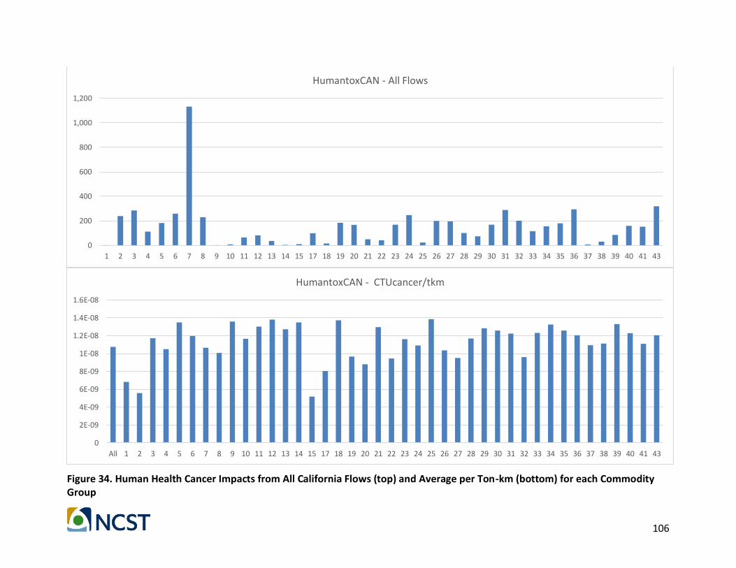
106

Figure 34. Human Health Cancer Impacts from All California Flows (top) and Average per Ton-km (bottom) for each Commodity Group

0

200

400

600

800

1,000

1,200

1 2 3 4 5 6 7 8 9 10 11 12 13 14 15 17 18 19 20 21 22 23 24 25 26 27 28 29 30 31 32 33 34 35 36 37 38 39 40 41 43

HumantoxCAN - All Flows

0

2E-09

4E-09

6E-09

8E-09

1E-08

1.2E-08

1.4E-08

1.6E-08

All 1 2 3 4 5 6 7 8 9 10 11 12 13 14 15 17 18 19 20 21 22 23 24 25 26 27 28 29 30 31 32 33 34 35 36 37 38 39 40 41 43

HumantoxCAN - CTUcancer/tkm

107

Figure 35. Human Health Non-Cancer Impacts from All California Flows (top) and Average per Ton-km (bottom) for each Commodity Group

0

2,000

4,000

6,000

8,000

10,000

12,000

1 2 3 4 5 6 7 8 9 10 11 12 13 14 15 17 18 19 20 21 22 23 24 25 26 27 28 29 30 31 32 33 34 35 36 37 38 39 40 41 43

HumantoxNC - All Flows

0

2E-08

4E-08

6E-08

8E-08

0.0000001

1.2E-07

1.4E-07

1.6E-07

All 1 2 3 4 5 6 7 8 9 10 11 12 13 14 15 17 18 19 20 21 22 23 24 25 26 27 28 29 30 31 32 33 34 35 36 37 38 39 40 41 43

HumantoxNC - CTUnoncanter/tkm

108

Figure 36. Global Warming Potential Impacts from All California Flows (top) and Average per Ton-km (bottom) for each Commodity Group

0

5,000

10,000

15,000

20,000

25,000

30,000

1 2 3 4 5 6 7 8 9 10 11 12 13 14 15 17 18 19 20 21 22 23 24 25 26 27 28 29 30 31 32 33 34 35 36 37 38 39 40 41 43

Mill

ion

sGWP - All Flows

0

0.2

0.4

0.6

0.8

1

1.2

All 1 2 3 4 5 6 7 8 9 10 11 12 13 14 15 17 18 19 20 21 22 23 24 25 26 27 28 29 30 31 32 33 34 35 36 37 38 39 40 41 43

GWP - kg CO2eq/tkm

109

Figure 37. Human Health Particulate Impacts from All California Flows (top) and Average per Ton-km (bottom) for each Commodity Group

0

5

10

15

20

25

30

1 2 3 4 5 6 7 8 9 10 11 12 13 14 15 17 18 19 20 21 22 23 24 25 26 27 28 29 30 31 32 33 34 35 36 37 38 39 40 41 43

Mill

ion

sHumanpartic - All Flows

0

0.00005

0.0001

0.00015

0.0002

0.00025

0.0003

0.00035

0.0004

All 1 2 3 4 5 6 7 8 9 10 11 12 13 14 15 17 18 19 20 21 22 23 24 25 26 27 28 29 30 31 32 33 34 35 36 37 38 39 40 41 43

Humanpartic - PM2.5eq/tkm

110

Figure 38. Ozone Depletion Potential Impacts from All California Flows (top) and Average per Ton-km (bottom) for each Commodity Group

0

1,000

2,000

3,000

4,000

5,000

6,000

7,000

1 2 3 4 5 6 7 8 9 10 11 12 13 14 15 17 18 19 20 21 22 23 24 25 26 27 28 29 30 31 32 33 34 35 36 37 38 39 40 41 43

ODP - All Flows

0

5E-08

0.0000001

1.5E-07

0.0000002

2.5E-07

0.0000003

All 1 2 3 4 5 6 7 8 9 10 11 12 13 14 15 17 18 19 20 21 22 23 24 25 26 27 28 29 30 31 32 33 34 35 36 37 38 39 40 41 43

ODP - kg CFC-11eq/tkm

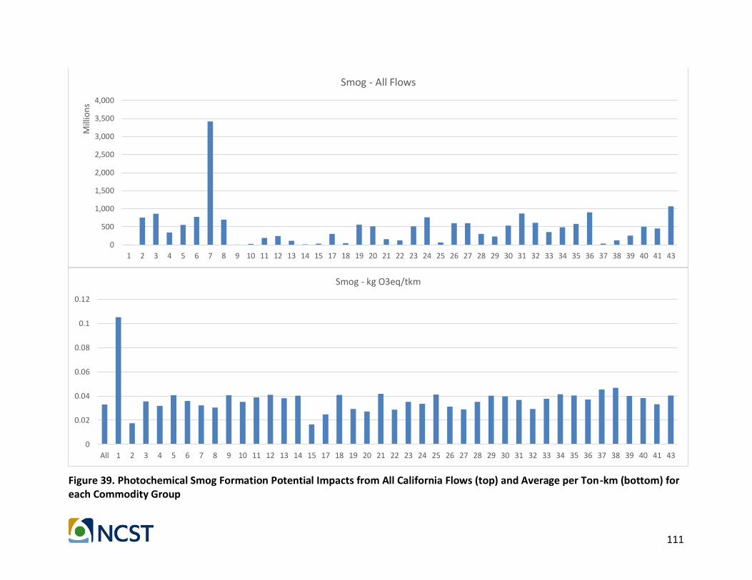
111

Figure 39. Photochemical Smog Formation Potential Impacts from All California Flows (top) and Average per Ton-km (bottom) for each Commodity Group

0

500

1,000

1,500

2,000

2,500

3,000

3,500

4,000

1 2 3 4 5 6 7 8 9 10 11 12 13 14 15 17 18 19 20 21 22 23 24 25 26 27 28 29 30 31 32 33 34 35 36 37 38 39 40 41 43

Mill

ion

sSmog - All Flows

0

0.02

0.04

0.06

0.08

0.1

0.12

All 1 2 3 4 5 6 7 8 9 10 11 12 13 14 15 17 18 19 20 21 22 23 24 25 26 27 28 29 30 31 32 33 34 35 36 37 38 39 40 41 43

Smog - kg O3eq/tkm

112

Figure 40. Acidification Potential Impacts from All California Flows (top) and Average per Ton-km (bottom) for each Commodity Group

0

20

40

60

80

100

120

140

160

1 2 3 4 5 6 7 8 9 10 11 12 13 14 15 17 18 19 20 21 22 23 24 25 26 27 28 29 30 31 32 33 34 35 36 37 38 39 40 41 43

Mill

ion

sAcidification - All Flows

0

0.0005

0.001

0.0015

0.002

0.0025

0.003

0.0035

0.004

0.0045

0.005

All 1 2 3 4 5 6 7 8 9 10 11 12 13 14 15 17 18 19 20 21 22 23 24 25 26 27 28 29 30 31 32 33 34 35 36 37 38 39 40 41 43

Acidification - kg SO2eq/tkm

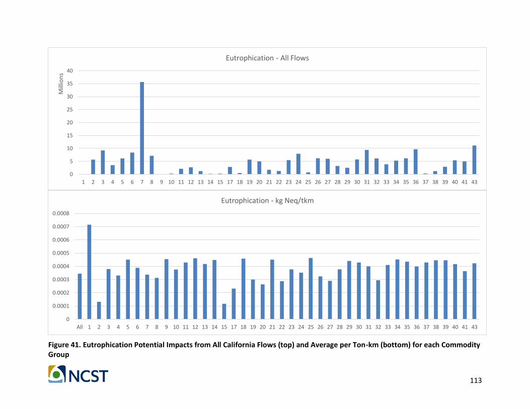
113

Figure 41. Eutrophication Potential Impacts from All California Flows (top) and Average per Ton-km (bottom) for each Commodity Group

0

5

10

15

20

25

30

35

40

1 2 3 4 5 6 7 8 9 10 11 12 13 14 15 17 18 19 20 21 22 23 24 25 26 27 28 29 30 31 32 33 34 35 36 37 38 39 40 41 43

Mill

ion

sEutrophication - All Flows

0

0.0001

0.0002

0.0003

0.0004

0.0005

0.0006

0.0007

0.0008

All 1 2 3 4 5 6 7 8 9 10 11 12 13 14 15 17 18 19 20 21 22 23 24 25 26 27 28 29 30 31 32 33 34 35 36 37 38 39 40 41 43

Eutrophication - kg Neq/tkm

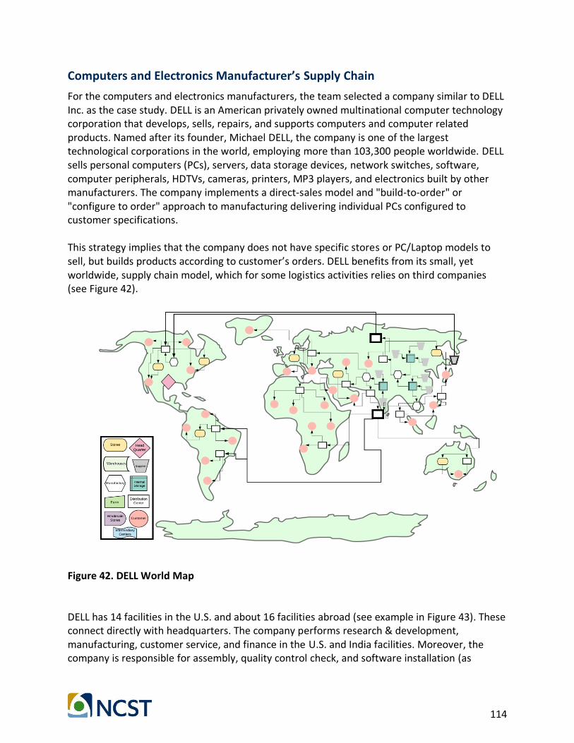
114

Computers and Electronics Manufacturer’s Supply Chain

For the computers and electronics manufacturers, the team selected a company similar to DELL Inc. as the case study. DELL is an American privately owned multinational computer technology corporation that develops, sells, repairs, and supports computers and computer related products. Named after its founder, Michael DELL, the company is one of the largest technological corporations in the world, employing more than 103,300 people worldwide. DELL sells personal computers (PCs), servers, data storage devices, network switches, software, computer peripherals, HDTVs, cameras, printers, MP3 players, and electronics built by other manufacturers. The company implements a direct-sales model and "build-to-order" or "configure to order" approach to manufacturing delivering individual PCs configured to customer specifications. This strategy implies that the company does not have specific stores or PC/Laptop models to sell, but builds products according to customer’s orders. DELL benefits from its small, yet worldwide, supply chain model, which for some logistics activities relies on third companies (see Figure 42).

Figure 42. DELL World Map DELL has 14 facilities in the U.S. and about 16 facilities abroad (see example in Figure 43). These connect directly with headquarters. The company performs research & development, manufacturing, customer service, and finance in the U.S. and India facilities. Moreover, the company is responsible for assembly, quality control check, and software installation (as

115

mentioned, other activities in the supply chain are outsourced). Figure 44 shows an example of DELL operations along a schematic of electronic products’ supply chain. DELL has realized that supply chain is becoming more and more important for the success of today’s business and they work accordingly to keep a competitive advantage in the market. The company has implemented supply chain management practices to develop an effective service from suppliers to consumers. Following the attributes discussed in Table 2, Table 24 shows the key aspects of DELL’s supply chain.

Figure 43. U.S. Map for DELL

Figure 44. DELL's Supply Chain

116

Table 24. DELL's Supply Chain Attributes

Procurement Type Number and type of products procured

Many (Sales over 62 billion $ in the first quarter of 2017)

Sourcing type Multiple (over 100 suppliers) Suppliers’ flexibility (Amounts to be supplied)

Low

Supplier lead time and reliability Low (Very Reliable)

Material’s life cycle Long

Production Type Organization of the production process

Job Shop

Repetition of operations Batch Production Changeover characteristics Sequence Dependent

Bottlenecks in production Could be both or none

Working time flexibility Multiple Shifts (Even 10h a day labor work)

Distribution Type Distribution structure One stage

Pattern of delivery Dynamic

Deployment of transportation means

Routes: Both (Variable & Standards) Capacity: Limited

Loading requirements: Applied for air and land transportation

Availability of future demands Forecasted

Demand curve Sporadic

Product’s life cycle nearly 20 years (LCA Study File) Number of product types 21 Product Type

Degree of customization Specific

Bill of materials (BOM) Convergent

Portion of service operations Tangible Products Typography of a supply chain

Network Structure Mixture

Degree of globalization Worldwide

Location of decoupling points Manufacture-to-order (Build in -to-order)

Major constraints Supplier, JIT production procedure

Integration and coordination

Legal position Inter-organizational

Balance of power Dominant Partner (Texas Headquarter) Direction of coordination Vertical

Major constraints All

To estimate the impacts of DELL’s freight flows, the research team conducted a comprehensive search for the specific company flows, but they were not publicly available. The team decided to conduct a market level analysis to allocate state flows (from the estimated CFS-PUM) to the company. In doing so, the team gathered information about market shares for PC makers around the world and in the U.S. Table 25 shows the global share of PC for six pioneering technological companies. These market shares only include desktop computers, laptops, and notebooks. The data shows that DELL has around 15% of total sales, and ranks third worldwide.

117

Table 25. Global PC Market Shares

Rank 2011 2012 2013 2014 2015 2016

1 HP 16.6 HP 16.1 Lenovo 16.9 Lenovo 18.8 Lenovo 19.8 Lenovo 20.7

2 Lenovo 12.5 Lenovo 14.9 HP 16.2 HP 17.5 HP 18.2 HP 19.4

3 DELL 11.7 DELL 10.7 DELL 11.6 DELL 12.8 DELL 13.6 DELL 14.7

4 Acer - Acer 10.2 Acer 8 Acer 7.9 Asus 7.3 Asus 7.6

5 Asus 5.7 Asus 6.9 Asus 6.6 Asus 7.2 Apple 7.2 Apple 6.9

Others 42.8 41.2 40.7 35.7 33.9 30.7

Source:(https://www.gartner.com/newsroom/id/3568420)

Moreover, Table 26 shows DELL’s worldwide quarterly market shares between 2011 and 2017. During the last year, the company increased the market in about half point. Table 26. DELL'S Worldwide Market Share (2011-2017)

Market share (in %)

Q1 '11 11.4

Q2 '11 12.1

Q3 '11 11.2

Q4 '11 12.2

Q1 '12 11 Q2 '12 11.3

Q3 '12 10.5

Q4 '12 10.4

Q1 '13 11.2

Q2 '13 11.9

Q3 '13 11.6

Q4 '13 11.8

Q1 '14 12.6

Q2 '14 13.3

Q3 '14 12.7 Q4 '14 13.1

Q1 '15 12.8

Q2 '15 14

Q3 '15 13.5

Q4 '15 13.5

Q1 '16 14.2

Q2 '16 14.7

Q3 '16 14.7

Q4 '16 14.8

Q1 '17 15 Q2 '17 15.6

Q3 '17 15.2

Q4 '17 15.2

Source: (https://www.statista.com/statistics/298976/pc-shipments-worldwide-dell-market-share/)

Although DELL’s share worldwide is around 15%, in the U.S., the company has had a share ranging between 20% and 26.2% between 2010 and 2016. Considering the CFS data available, the team estimated an average market share for the company of 21.33% (see Table 27 for U.S. quarterly shares). Detailed data at the State level was not available.

118

Table 27. PC Unit Shipments in the U.S. - DELL's Quarterly Market Share 2010-2016

Market share (in %)

Q1 '10 23.4

Q2 '10 23.7 Q3 '10 23.6

Q4 '10 22

Q1 '11 22.7

Q2 '11 22.2

Q3 '11 21.6

Q4 '11 22.4

Q1 '12 22.1

Q2 '12 22.5

Q3 '12 20.7

Q4 '12 20 Q1 '13 21.7

Q2 '13 24.3

Q3 '13 20.9

Q4 '13 21.9

Q1 '14 24.2

Q2 '14 25.4

Q3 '14 23.9

Q4 '14 23.1

Q1 '15 23.1

Q2 '15 24.1 Q3 '15 24.1

Q4 '15 23.9

Q1 '16 25.6

Q2 '16 25.8

Q3 '16 26.2

Source: (https://www.statista.com/statistics/311417/us-pc-unit-shipments-dell-market-share/)

Considering that the CFS-PUM data contained information about both the industry category and the transported commodities, the team identified DELL’s NAICS and the type of products it sells and distributes. DELL’s NAICS codes are 423430 and 33411 (DELL Inc. is also found in NAICS 443142: Electronic stores); however, the company distributes a range of commodities that may not be all commodities transported by establishments in this NAICS code. There was an additional limitation to the existing data. The NAICS code was restricted to 3- or 4-digits in the data, and the commodities only at the 2-digit SCTG. Overall, the company belongs to the following subsectors:

Sector 42: Wholesale Trade ✓ Subsector 423: Merchant Wholesalers, Durable Goods

o Industry Group 4234: Professional and Commercial Equipment and Supplies Merchant Wholesalers ▪ Industry 42343: Computer and Computer Peripheral Equipment and

Software Merchant Wholesalers

• 6 Digit Code(s) NAICS 423430: Computer and Computer Peripheral Equipment and Software Merchant Wholesalers

Sector 31-33: Manufacturing ✓ Subsector 334: Computer and Electronic Product Manufacturing

o Industry Group 3341: Computer and Peripheral Equipment Manufacturing o Industry 33411: Computer and Peripheral Equipment Manufacturing

▪ 6 Digit Code(s) NAICS 334111: Electronic Computer Manufacturing ▪ 6 Digit Code(s) NAICS 334112: Computer Storage Device Manufacturing ▪ 6 Digit Code(s) NAICS 334118: Computer Terminal and Other Computer

Peripheral Equipment Manufacturing ▪ 6 Digit Code(s) NAICS 33411A: Computer terminals and other computer

peripheral equipment manufacturing

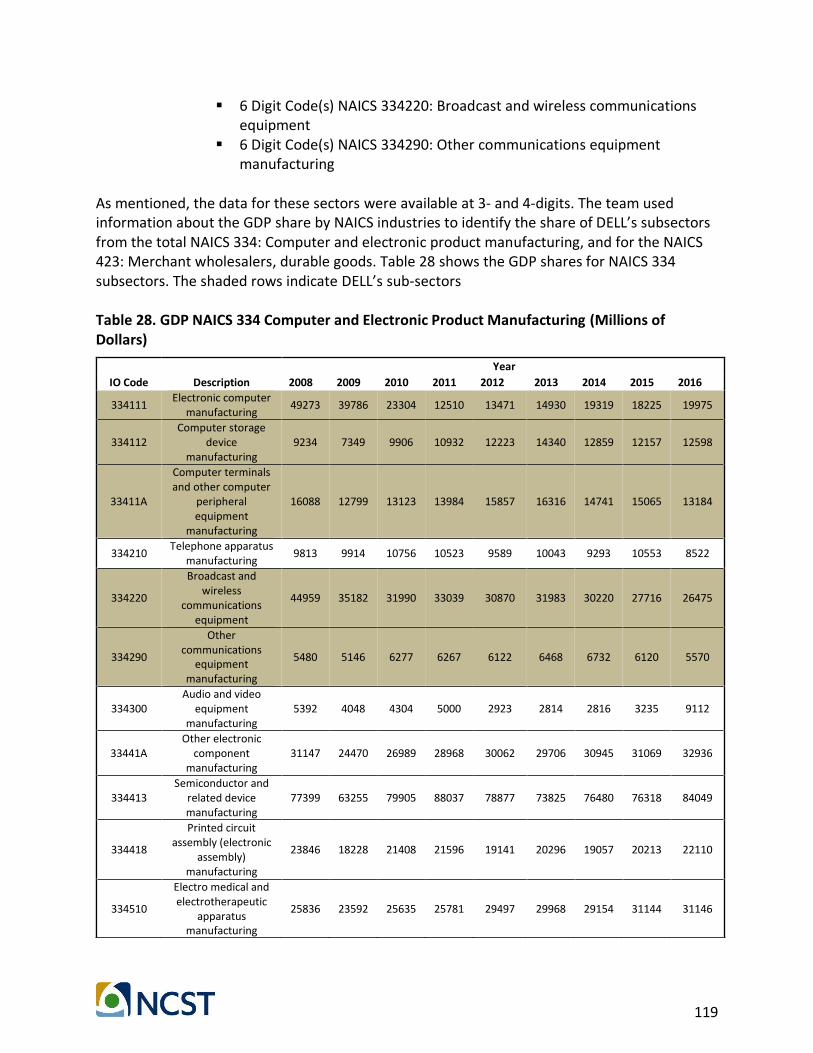
119

▪ 6 Digit Code(s) NAICS 334220: Broadcast and wireless communications equipment

▪ 6 Digit Code(s) NAICS 334290: Other communications equipment manufacturing

As mentioned, the data for these sectors were available at 3- and 4-digits. The team used information about the GDP share by NAICS industries to identify the share of DELL’s subsectors from the total NAICS 334: Computer and electronic product manufacturing, and for the NAICS 423: Merchant wholesalers, durable goods. Table 28 shows the GDP shares for NAICS 334 subsectors. The shaded rows indicate DELL’s sub-sectors Table 28. GDP NAICS 334 Computer and Electronic Product Manufacturing (Millions of Dollars)

Year

IO Code Description 2008 2009 2010 2011 2012 2013 2014 2015 2016

334111 Electronic computer

manufacturing 49273 39786 23304 12510 13471 14930 19319 18225 19975

334112 Computer storage

device manufacturing

9234 7349 9906 10932 12223 14340 12859 12157 12598

33411A

Computer terminals and other computer

peripheral equipment

manufacturing

16088 12799 13123 13984 15857 16316 14741 15065 13184

334210 Telephone apparatus

manufacturing 9813 9914 10756 10523 9589 10043 9293 10553 8522

334220

Broadcast and wireless

communications equipment

44959 35182 31990 33039 30870 31983 30220 27716 26475

334290

Other communications

equipment manufacturing

5480 5146 6277 6267 6122 6468 6732 6120 5570

334300 Audio and video

equipment manufacturing

5392 4048 4304 5000 2923 2814 2816 3235 9112

33441A Other electronic

component manufacturing

31147 24470 26989 28968 30062 29706 30945 31069 32936

334413 Semiconductor and

related device manufacturing

77399 63255 79905 88037 78877 73825 76480 76318 84049

334418

Printed circuit assembly (electronic

assembly) manufacturing

23846 18228 21408 21596 19141 20296 19057 20213 22110

334510

Electro medical and electrotherapeutic

apparatus manufacturing

25836 23592 25635 25781 29497 29968 29154 31144 31146

120

Year

IO Code Description 2008 2009 2010 2011 2012 2013 2014 2015 2016

334511

Search, detection, and navigation

instruments manufacturing

52422 52303 53358 54461 52796 50452 48873 50401 51619

334512

Automatic environmental

control manufacturing

3451 2931 3249 3164 3196 3214 3315 3076 3259

334513 Industrial process

variable instruments manufacturing

11008 9132 9662 10974 12858 12965 13481 12866 13641

334514 Totalizing fluid meter and counting device

manufacturing 5942 5180 6050 6756 6964 5982 5565 5482 5774

334515 Electricity and signal testing instruments

manufacturing 11989 9060 10111 10828 12892 12092 12050 11700 12176

334516 Analytical laboratory

instrument manufacturing

14345 12877 14197 14666 15009 14939 17670 17938 19108

334517 Irradiation apparatus

manufacturing 4499 4217 4307 4102 10548 12220 11814 13452 12986

33451A

Watch, clock, and other measuring and

controlling device manufacturing

10588 8887 9480 10968 12821 13182 13109 12214 12890

334610

Manufacturing and reproducing

magnetic and optical media

6945 5073 4691 3790 3611 3231 3391 3505 3027

Total 19656 53429 68702 76346 79327 78966 80884 82449 400157

Share of Computer and electronics

0.177 0.169 0.125 0.099 0.207 0.120 0.123 0.119 0.114

Source: (Bureau of Economic Analysis, 2017)

According to the estimates, the share of computers and electronic in NAICS code 334 is about 20% of the GDP. Obviously, the share of DELL is much lower than this since the company is just one of many companies in the industry. Similarly, according to the total value of shipments, Figure 45 shows the 2012 share for different industries in GDP. The industries in the figure include all the NAICS sub-category codes, which means that for the computer and electronic products, the 7% also includes all 334 NAICS code, or even more.

121

Figure 45. Industries by their Value of Shipments (Bureau of Economic Analysis, 2017)

Considering that the team could not identify NAICS 423 disaggregate data, and the primary NAICS code is 334111, the latter’s market shared served as the representative for the analyses.

Food Producer’s Supply Chain

For a food producer, the team used Nestlé as a reference. Nestlé is Switzerland's largest company and the world's largest consumer food company, founded by Henri Nestlé in 1867. Today, it is valued at over $76 billion, and employs 253,000 people from more than 70 countries. Nestlé produces more than 15,000 different products. Nestle merged with the Anglo-Swiss Condensed Milk Company in 1905. Nestlé follows the principle of decentralization, which means each country is responsible for the efficient running of its business. Currently, the company operates in over 77 countries with 480 factories. Figure 46 and Figure 47 show simplified flow charts of the company’s supply chain worldwide and in the U.S., respectively.

Chemical14%

Food13%

Transportation

Equipment13%

Petroleum and Coal Products

13%

Computer and electronics Products

7%

Machinery7%

Fabricated metal Products

6%

Primary Metal5%

Plastics and Rubber products

4%

Paper3%

Others15%

122

Figure 46. Nestlé World Map

Figure 47. U.S. Map for Nestlé

Moreover, Figure 48 shows a process flow for Nestlé operations along the supply chain. Table

29 provide additional details about the company’s supply chain attributes.

123

Figure 48. Nestlé Supply Chain

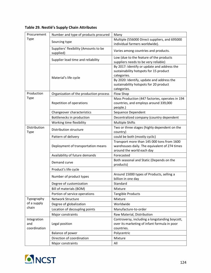
124

Table 29. Nestlé’s Supply Chain Attributes

Procurement Type

Number and type of products procured Many

Sourcing type Multiple (556000 Direct suppliers, and 695000 individual farmers worldwide).

Suppliers’ flexibility (Amounts to be supplied)

Varies among countries and products.

Supplier lead time and reliability Low (due to the feature of the products suppliers needs to be very reliable)

Material’s life cycle

By 2017: Identify or update and address the sustainability hotspots for 15 product categories.

By 2020: Identify, update and address the sustainability hotspots for 20 product categories.

Production Type

Organization of the production process Flow Shop

Repetition of operations Mass Production (447 factories, operates in 194 countries, and employs around 339,000 people.)

Changeover characteristics Sequence Dependent

Bottlenecks in production Decentralized company (country dependent

Working time flexibility Multiple Shifts

Distribution Type

Distribution structure Two or three stages (highly dependent on the country)

Pattern of delivery could be both (mostly cyclic)

Deployment of transportation means Transport more than 145 000 tons from 1600 warehouses daily. The equivalent of 274 times around the world each day

Availability of future demands Forecasted

Demand curve Both seasonal and Static (Depends on the products)

Product’s life cycle

Number of product types Around 15000 types of Products, selling a billion in one day

Degree of customization Standard

Bill of materials (BOM) Mixture

Portion of service operations Tangible Products

Typography of a supply chain

Network Structure Mixture

Degree of globalization Worldwide

Location of decoupling points Manufacture-to-order

Major constraints Raw Material, Distribution

Integration and coordination

Legal position Controversy, including a longstanding boycott, over its marketing of infant formula in poor countries.

Balance of power Polycentric

Direction of coordination Mixture

Major constraints All

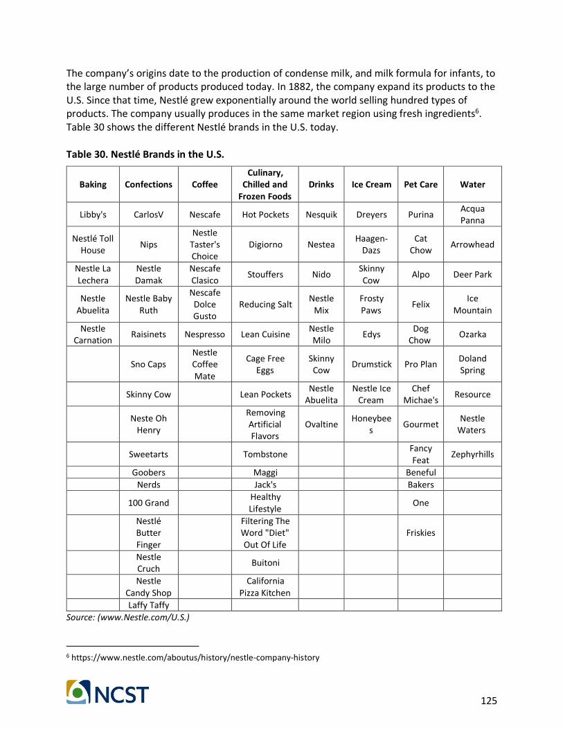
125

The company’s origins date to the production of condense milk, and milk formula for infants, to the large number of products produced today. In 1882, the company expand its products to the U.S. Since that time, Nestlé grew exponentially around the world selling hundred types of products. The company usually produces in the same market region using fresh ingredients6. Table 30 shows the different Nestlé brands in the U.S. today. Table 30. Nestlé Brands in the U.S.

Baking Confections Coffee Culinary,

Chilled and Frozen Foods

Drinks Ice Cream Pet Care Water

Libby's CarlosV Nescafe Hot Pockets Nesquik Dreyers Purina Acqua Panna

Nestlé Toll House

Nips Nestle

Taster's Choice

Digiorno Nestea Haagen-

Dazs Cat

Chow Arrowhead

Nestle La Lechera

Nestle Damak

Nescafe Clasico

Stouffers Nido Skinny Cow

Alpo Deer Park

Nestle Abuelita

Nestle Baby Ruth

Nescafe Dolce Gusto

Reducing Salt Nestle

Mix Frosty Paws

Felix Ice

Mountain

Nestle Carnation

Raisinets Nespresso Lean Cuisine Nestle Milo

Edys Dog

Chow Ozarka

Sno Caps Nestle Coffee Mate

Cage Free Eggs

Skinny Cow

Drumstick Pro Plan Doland Spring

Skinny Cow Lean Pockets Nestle

Abuelita Nestle Ice

Cream Chef

Michae's Resource

Neste Oh

Henry

Removing Artificial Flavors

Ovaltine Honeybee

s Gourmet

Nestle Waters

Sweetarts Tombstone Fancy Feat

Zephyrhills

Goobers Maggi Beneful

Nerds Jack's Bakers

100 Grand Healthy Lifestyle

One

Nestlé Butter Finger

Filtering The Word "Diet" Out Of Life

Friskies

Nestle Cruch

Buitoni

Nestle

Candy Shop

California Pizza Kitchen

Laffy Taffy

Source: (www.Nestle.com/U.S.)

6 https://www.nestle.com/aboutus/history/nestle-company-history

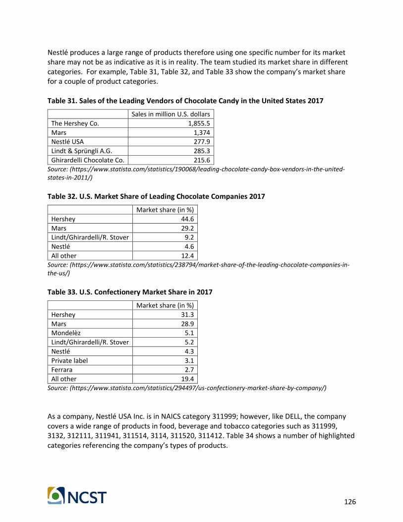
126

Nestlé produces a large range of products therefore using one specific number for its market share may not be as indicative as it is in reality. The team studied its market share in different categories. For example, Table 31, Table 32, and Table 33 show the company’s market share for a couple of product categories. Table 31. Sales of the Leading Vendors of Chocolate Candy in the United States 2017

Sales in million U.S. dollars

The Hershey Co. 1,855.5

Mars 1,374 Nestlé USA 277.9

Lindt & Sprüngli A.G. 285.3

Ghirardelli Chocolate Co. 215.6 Source: (https://www.statista.com/statistics/190068/leading-chocolate-candy-box-vendors-in-the-united-states-in-2011/)

Table 32. U.S. Market Share of Leading Chocolate Companies 2017

Market share (in %)

Hershey 44.6

Mars 29.2

Lindt/Ghirardelli/R. Stover 9.2

Nestlé 4.6

All other 12.4 Source: (https://www.statista.com/statistics/238794/market-share-of-the-leading-chocolate-companies-in-the-us/)

Table 33. U.S. Confectionery Market Share in 2017

Market share (in %)

Hershey 31.3

Mars 28.9 Mondelèz 5.1

Lindt/Ghirardelli/R. Stover 5.2

Nestlé 4.3

Private label 3.1 Ferrara 2.7

All other 19.4 Source: (https://www.statista.com/statistics/294497/us-confectionery-market-share-by-company/)

As a company, Nestlé USA Inc. is in NAICS category 311999; however, like DELL, the company covers a wide range of products in food, beverage and tobacco categories such as 311999, 3132, 312111, 311941, 311514, 3114, 311520, 311412. Table 34 shows a number of highlighted categories referencing the company’s types of products.

127

Table 34. Nestlé NIACS Subcategories

NAICS Description

311 Food and beverage and tobacco products 311111 Dog and cat food manufacturing

311119 Other animal food manufacturing

311210 Flour milling and malt manufacturing

311221 Wet corn milling 31122A Soybean and other oilseed processing

311225 Fats and oils refining and blending

311230 Breakfast cereal manufacturing

311300 Sugar and confectionery product manufacturing

311410 Frozen food manufacturing

311420 Fruit and vegetable canning, pickling, and drying

31151A Fluid milk and butter manufacturing

311513 Cheese manufacturing

311514 Dry, condensed, and evaporated dairy product manufacturing

311520 Ice cream and frozen dessert manufacturing 31161A Animal (except poultry) slaughtering, rendering, and processing

311615 Poultry processing

311700 Seafood product preparation and packaging 311810 Bread and bakery product manufacturing

3118A0 Cookie, cracker, pasta, and tortilla manufacturing

311910 Snack food manufacturing

311920 Coffee and tea manufacturing 311930 Flavoring syrup and concentrate manufacturing

311940 Seasoning and dressing manufacturing

311990 All other food manufacturing

312110 Soft drink and ice manufacturing 312120 Breweries

312130 Wineries

312140 Distilleries

312200 Tobacco product manufacturing 313TT Textile mills and textile product mills

313100 Fiber, yarn, and thread mills

313200 Fabric mills

313300 Textile and fabric finishing and fabric coating mills

314110 Carpet and rug mills

314120 Curtain and linen mills

314900 Other textile product mills

42 Wholesale trade

423000 Merchant wholesalers, durable goods

424000 Merchant wholesalers, nondurable goods

425000 Wholesale electronic markets and agents and brokers

42XXXX Wholesale trade adjustments

423000 Merchant wholesalers, durable goods

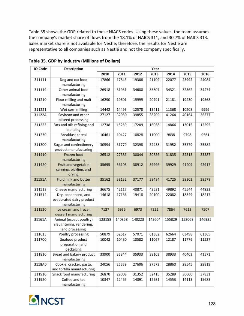
128

Table 35 shows the GDP related to these NIACS codes. Using these values, the team assumes the company’s market share of flows from the 18.1% of NAICS 311, and 30.7% of NAICS 313. Sales market share is not available for Nestlé; therefore, the results for Nestlé are representative to all companies such as Nestlé and not the company specifically. Table 35. GDP by Industry (Millions of Dollars)

IO Code Description Year

2010 2011 2012 2013 2014 2015 2016

311111 Dog and cat food manufacturing

17866 17845 19388 21109 22077 23992 24084

311119 Other animal food manufacturing

26918 31951 34680 35807 34321 32362 34474

311210 Flour milling and malt manufacturing

16290 19601 19999 20791 21181 19230 19568

311221 Wet corn milling 14442 14493 12578 13411 11368 10208 9999

31122A Soybean and other oilseed processing

27127 32950 39855 38209 41264 40164 36377

311225 Fats and oils refining and blending

12738 15259 17289 16058 14866 13015 12595

311230 Breakfast cereal manufacturing

10461 10427 10828 11000 9838 9798 9561

311300 Sugar and confectionery product manufacturing

30594 31779 32398 32458 31952 35379 35382

311410 Frozen food manufacturing

26512 27386 30044 30856 31835 32313 33387

311420 Fruit and vegetable canning, pickling, and

drying

35695 36103 38912 39996 39929 41409 42917

31151A Fluid milk and butter manufacturing

35162 38132 37177 38484 41725 38302 38578

311513 Cheese manufacturing 36675 42117 40871 43531 49892 45544 44933

311514 Dry, condensed, and evaporated dairy product

manufacturing

14618 17166 19418 20100 22082 18349 18217

311520 Ice cream and frozen dessert manufacturing

7137 6935 6973 7322 7864 7613 7507

31161A Animal (except poultry) slaughtering, rendering,

and processing

123158 140858 140223 142604 155829 152069 146935

311615 Poultry processing 50879 52617 57071 61382 62664 63498 61365

311700 Seafood product preparation and

packaging

10042 10480 10582 11067 12187 11776 11537

311810 Bread and bakery product manufacturing

33900 35344 35933 38103 38933 40402 41571

3118A0 Cookie, cracker, pasta, and tortilla manufacturing

24056 25339 27606 27572 28860 28545 29819

311910 Snack food manufacturing 26870 29008 31352 32415 35289 36600 37831

311920 Coffee and tea manufacturing

10347 12465 14091 12931 14553 14113 15683

129

IO Code Description Year

2010 2011 2012 2013 2014 2015 2016

311930 Flavoring syrup and concentrate

manufacturing

9059 9739 8950 8997 10485 8386 10496

311940 Seasoning and dressing manufacturing

16599 17281 18975 19662 19303 19955 20255

311990 All other food manufacturing

20289 20744 21987 23622 24824 27244 27488

Share of Nestle in 311 Code 0.189 0.180 0.181 0.182 0.179 0.181 0.185

313TT Textile mills and textile product mills

313100 Fiber, yarn, and thread mills

6935 7594 7803 8104 8208 7955 7885

313200 Fabric mills 14719 15212 14710 15110 14973 14570 14200

313300 Textile and fabric finishing and fabric coating mills

7661 7914 7474 8148 8194 8530 8243

314110 Carpet and rug mills 7745 8870 9036 9373 9848 9539 10149

314120 Curtain and linen mills 3651 3708 3580 3549 4375 4190 4704

314900 Other textile product mills 9161 9140 9145 9665 10603 10766 12336

313100 Fiber, yarn, and thread mills

6935 7594 7803 8104 8208 7955 7885

Share of Nestle in 313 Code 0.323 0.315 0.307 0.301 0.300 0.295 0.289

*Source: (Bureau of Economic Analysis, 2017)

Apparel/Shoes Manufacturer’s Supply Chain

In this case study, the team selected Nike Inc. as an example of an apparel and shoes manufacturer for the illustrative company. Nike Inc. is a worldwide producer of athletic apparel and shoes, and is a recognized multinational corporation. In 2012, Nike had almost 44,000 employees worldwide and its revenue in 2017 was $34.4 billion. Nike has more than 20 brands including shoes, apparel and equipment around the world (https://www.kicksonfire.com/history-of-nike/). Figure 49 and Figure 50 show simplified flow charts for the worldwide and U.S. supply chains. The company has been outsourcing and getting materials from suppliers all around the world.

130

Figure 49. Nike World Map

Figure 50. U.S. Map for Nike Figure 51 and Table 36 show the company’s operations along the supply chain, and details about the supply chain structures, respectively. Nike’s types of products are different from the previous two case studies. The supply chain is also diverse, as it has production facilities scattered all around the world due to high demand. Suppliers are outsourced and they all agree to terms of service of Nike that mostly emphasize on Green production. After a number of media backlashes, the company has invested efforts to preserve the environment. Distribution

131

and sales mostly happen through third parties; however, there are many Nike stores, which are under direct supervision of the company7.

Figure 51. Nike Supply Chain

7 https://www.kicksonfire.com/history-of-nike/)

132

Table 36. Nike's Supply Chain Structure

Procurement Type Number and type of products procured

120,000,000 Nike shoes each year (Annual sale of 32.46 billion$ in 2016)

Sourcing type Multiple (Rubber, Fabric, etc.) Suppliers’ Multiple (Rubber, Fabric, etc.)

Supplier lead time and reliability Long (Less reliable)

Material’s life cycle Long

Production Type Organization of the production process

Flow shop (it mostly depends due to the different factories and products)

Repetition of operations Mass Production

Changeover characteristics Sequence Dependent Bottlenecks in production Raw Materials (Inventory control…)

Working time flexibility Multiple Shifts

Distribution Type Distribution structure Three stage (out-sourced)

Pattern of delivery Cyclic

Deployment of transportation means

Routes: Standards

Capacity: Limited Loading Requirements: Applied for Truck and air Transportation

Availability of future demands Forecasted

Demand curve Static (Due to the historical data and huge network of distributers)

Product’s life cycle - Number of product types 500000 types of products

Degree of customization Highly specific

Bill of materials (BOM) Mixture

Portion of service operations Tangible Product Typography of a supply chain

Network Structure Mixture

Degree of globalization Worldwide

Location of decoupling points Engineer-to-order Major constraints Inventory Control

Integration and coordination

Legal position Inter-organizational

Balance of power Dominant Partner (Oregon Headquarter)

Direction of coordination Vertical integration Major constraints All

Table 37 and Table 38 show the historic and forecasted company’s market share in the footwear and apparel industry segments. The data for footwear is worldwide, whereas the apparel share data is for the U.S.

133

Table 37. Forecast of Nike's Global Market Share in Athletic Footwear from 2011 to 2024

Global market share

2011 16.77

2012 18.39

2013 19.66

2014 22.49

2015 23.95

2016 25.01

2017 26.01

2018 27.51

2019 29.01

2020 30.51

2021 32.01

2022 33.01

2023 34.01

2024 35.01 Source:(https://www.statista.com/statistics/216821/forecast-for-nikes-global-market-share-in-athletic-footwear-until-2017/)

Table 38. Market Share of the Leading Brand Apparel Companies in the United States in 2016

Apparel Company Market share (in %)

Gap 4

Wal-Mart 3.5

Nike 2.7

Hanesbrands 2.5

L Brands 2.3

VF 2.1

PVH 2.1

Under Armour 1.7

Target 1.7

Forever 21 1.6 Source: (https://www.statista.com/statistics/734460/leading-brand-apparel-companies-market-share-us/)

As a company, Nike is in the NAICS 316210 industry category; however, like the other case studies, the wide range of products come under different NAICS codes. Unlike to NAICS code 311, apparel-manufacturing code related to Nike “339” only has eleven subsections (see Table 39).

134

Table 39. NICS 339 Subcategories

NAICS Description 339 Miscellaneous manufacturing

339112 Surgical and medical instrument manufacturing 339113 Surgical appliance and supplies manufacturing 339114 Dental equipment and supplies manufacturing 339115 Ophthalmic goods manufacturing 339116 Dental laboratories 339910 Jewelry and silverware manufacturing 339920 Sporting and athletic goods manufacturing 339930 Doll, toy, and game manufacturing 339940 Office supplies (except paper) manufacturing 339950 Sign manufacturing 339990 All other miscellaneous manufacturing

Table 40 shows the GDP shares for NAICS 339. Table 40. GDP by Industry (Millions of Dollars)

IO Code Description Year

2010 2011 2012 2013 2014 2015 2016

339112 Surgical and medical

instrument manufacturing

36321 37206 37498 40479 38429 39371 36402

339113 Surgical appliance

and supplies manufacturing

38042 37475 36926 40287 37563 37810 35608

339114 Dental equipment

and supplies manufacturing

4924 5200 4923 5237 4337 5015 4296

339115 Ophthalmic goods

manufacturing 4742 5730 6772 7167 6887 6810 6344

339116 Dental laboratories 4885 4827 5410 5899 5694 5432 5340

339910 Jewelry and silverware

manufacturing 8677 8123 7830 8185 9088 8359 8289

339920 Sporting and

athletic goods manufacturing

9995 10126 10036 10281 10266 10898 10391

339930 Doll, toy, and game

manufacturing 2720 2561 1700 1518 1763 1902 1699

339940 Office supplies (except paper) manufacturing

4186 4229 2674 2599 2903 3122 3034

339950 Sign manufacturing 11730 11926 11965 12758 13765 15053 13746

339990 All other

miscellaneous manufacturing

28094 29491 28468 28643 29730 32797 29128

135

IO Code Description Year

2010 2011 2012 2013 2014 2015 2016

Share of Nike related code in NAICS 339

0.064 0.064 0.065 0.063 0.063 0.065 0.067

Source: (Bureau of Economic Analysis, 2017)

The table shows that the share of Sport and athletic goods manufacturing in NIACS 339 is 6.5%, which relates to Nike’s products; however, 6.5% is reflecting all the sports goods companies and industries (in terms of Value) and the share of NIKE is not yet determined. Because Nike is a very large enterprise and covers varieties of products, there is a specific NAICS code for its Footwear manufacturing, which is 316210 (https://www.manta.com/c/mmn5xvn/nike-usa-inc, n.d.). However, there is no share information for this specific code. The team considered the general NAICS industry 316 (see Table 41). Table 42 shows the GDP for NAICS 339. In general, all companies like Nike have a share in terms of value of the goods of 6.5% for NAICS 339 and 2.34% for NAICS 315AL. These shares are for all the companies that are producing sportswear and goods and not NIKE itself. In order to have a better sense of NIKE’s real share, the team considered its market share among other sportswear companies, which in the U.S. was 48% in 2014. Table 41. NICS 315AL Subcategories

315AL Apparel and leather and allied products 315000 Apparel manufacturing 316000 Leather and allied product manufacturing

Table 42. GDP by Industry (Millions of Dollars)

IO Code Description Year

2010 2011 2012 2013 2014 2015 2016

339112 Surgical and medical

instrument manufacturing 36321 37206 37498 40479 38429 39371 36402

339113 Surgical appliance and

supplies manufacturing 38042 37475 36926 40287 37563 37810 35608

Share of Nike related code in NAICS 315AL

0.313 0.312 0.234 0.235 0.215 0.235 0.175

Source: (Bureau of Economic Analysis, 2017)

Company’s Summary and LCA Analyses

The previous sections showed important information to help determine the market share for these companies. As discussed, for some of these, the research team could not identify the specific market share, thus the results may correspond to industry level representative companies in the electronics, footwear and apparel, and consumer goods. Table 43 summarizes the various shares, at the company, and at the industry level considering the types of sub-sectors. For example, the 48% Nike market share corresponds to the available information about sneakers sales in the U.S. Moreover, Table 43 shows the commodity types associated to

136

the shipments of the representative companies. These values help filter the shipments from the industry level shipments provided by the CFS-PUM. The team used the data to estimate the ton-kms per mode and allocated them to the different companies. Table 43. Summary Market Shares and Commodities Associated to the Companies

DELL Nestlé Nike

Market Share

21.30% 20% 48%

Industry Shares

NAICS Code

334 311 313 339 316

% share 20.70% 18.10% 30.70% 6.50% 23.40%

SCTG Commodities

35 29 1 6

38 30 2 7

3 8

4 9

5

Source: (https://www.statista.com/)

Figure 52 shows the total inbound and outbound estimated shipments for these companies or representative businesses. The majority of the flows use for-hire trucks and parcel. Nestlé transports around 30% of the shipments using rail, while DELL uses air for 15 to 25% of the shipments.

137

Figure 52. Inbound and Outbound Total Shipments per Mode (top), and Mode Share (bottom)

Figure 53 shows the average per ton-kms TRACI impacts for the various companies. These results are consistent with the mode shares. As expected, the higher share of rail shipments translates in reduced per unit (ton-km) for Nestlé. Moreover, the use of air shipments by DELL

-

100

200

300

400

500

600

700

800

900

1,000

Dell Nestle Nike

Mill

ion

sInbound

-

200

400

600

800

1,000

1,200

1,400

Dell Nestle Nike

Mill

ion

s

Outbound

0%

10%

20%

30%

40%

50%

60%

70%

80%

90%

100%

Dell Nestle Nike

Inbound

Water (Deep Sea, Inland waterways)

Truck multimodal

For-hire truck

Private truck

Parcel, USPS, or courier

Rail

Air

0%

10%

20%

30%

40%

50%

60%

70%

80%

90%

100%

Dell Nestle Nike

Outbound

Water (Deep Sea, Inland waterways)

Truck multimodal

For-hire truck

Private truck

Parcel, USPS, or courier

Rail

Air

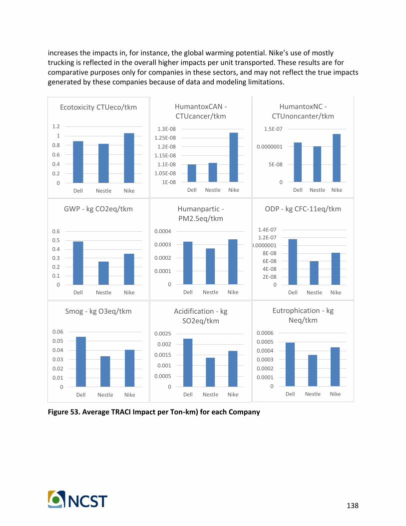
138

increases the impacts in, for instance, the global warming potential. Nike’s use of mostly trucking is reflected in the overall higher impacts per unit transported. These results are for comparative purposes only for companies in these sectors, and may not reflect the true impacts generated by these companies because of data and modeling limitations.

Figure 53. Average TRACI Impact per Ton-km) for each Company

0

0.2

0.4

0.6

0.8

1

1.2

Dell Nestle Nike

Ecotoxicity CTUeco/tkm

1E-08

1.05E-08

1.1E-08

1.15E-08

1.2E-08

1.25E-08

1.3E-08

Dell Nestle Nike

HumantoxCAN -CTUcancer/tkm

0

5E-08

0.0000001

1.5E-07

Dell Nestle Nike

HumantoxNC -CTUnoncanter/tkm

0

0.1

0.2

0.3

0.4

0.5

0.6

Dell Nestle Nike

GWP - kg CO2eq/tkm

0

0.0001

0.0002

0.0003

0.0004

Dell Nestle Nike

Humanpartic -PM2.5eq/tkm

0

2E-08

4E-08

6E-08

8E-08

0.0000001

1.2E-07

1.4E-07

Dell Nestle Nike

ODP - kg CFC-11eq/tkm

0

0.01

0.02

0.03

0.04

0.05

0.06

Dell Nestle Nike

Smog - kg O3eq/tkm

0

0.0005

0.001

0.0015

0.002

0.0025

Dell Nestle Nike

Acidification - kg SO2eq/tkm

0

0.0001

0.0002

0.0003

0.0004

0.0005

0.0006

Dell Nestle Nike

Eutrophication - kg Neq/tkm

139

IX. Conclusions

During the last few years, the freight transportation system has received increased attention from researchers, practitioners, and public agencies. Last year, the Governor’s Office released the CSFAP that seeks to improve freight efficiency in the State. The CSFAP will assess freight efficiency by changes in the CO2eq emissions per contribution to the economy from the transportation sector defined as NAICS 48 and 49 (transportation and warehousing services minus passenger transport). The research reported in this document developed a framework to conceptualize the freight system and assess the impacts (Freight System Conceptualization and Impact Assessment Framework). Specifically, the framework is a commodity-based framework that assesses the environmental impacts of freight flows. The framework can aid decision-making and provides a base description of the impacts resulting from inbound and outbound freight flows for a number of industry sectors (not only NAICS 48-49), commodity groups, and modes of transport. The authors developed the framework using LCA as the basis. During the process, the team identified a number of existing data and modeling limitations to implement such a framework at a larger scale. In addition to the limitations discussed in the document, the team identified a shortcoming of efficiency measures focusing on specific industry sectors and stakeholders. Discussing the relationship between the different stakeholders in the freight sector, Jaller et al. (2016a) argue that in many sectors, carrier companies and other supporting facilities (NAICS 48 and 49), do not have the necessary market power to affect freight and logistics decisions. These decisions are ultimately the ones that determine the shipment sizes, distances, frequency of distribution, and mode of transport, among others. Essentially, these ones affect the efficiency of the freight transportation system. In general, carrier companies are just a conduit between the economic agents responsible for those decisions. Therefore, measuring freight efficiency on the carriers (and warehouses) operations does not necessarily translate into overall freight system improvements. Given the market forces and other system constraints, these agents may only have a limited number of options to improve their operations (movement of the cargo). These are, in many cases, only related to technological improvements (changes in drivetrain, powertrain, fuel pathway), and some logistics changes to optimize routes, and ecological driving type of strategies. However, these might only optimize parts of the freight supply chain (i.e., transportation component) and do not necessarily achieve a system optimum. Moreover, there may be unintended consequences to specific stakeholders resulting from the selection of strategies by a sub-set of the economic agents. These impacts are not fully understood. For instance, the research evidenced a lack of tools to assess the impacts of freight vehicles on the infrastructure, and adequate allocation criteria for the different segments of the freight industry and the types of infrastructure. The analyses also show the need for additional research to understand and assess responsibility for the impacts generated by freight movements. Two different perspectives could result in different analyses for the State flows LCA estimates. For example, the results per industry show the impact of the flows generated by the establishments form these industries; however, the vehicles and carrier companies in NAICS 48 (with the exception of private trucks, which are

140

mostly operated by the company) generate these impacts. The emerging questions is about how to allocate the impacts, should they be allocated to the generating company or the hired carrier? Moreover, the results show that only concentrating in NAICS 48-49 may not include the ~10% impacts from the flows transported by the establishments, which are not included in the NAICS 48 flows (see Table 44). Table 44. Comparative Impacts per Mode for All California Flows

Eco

toxi

city

Hu

man

toxC

AN

Hu

man

toxN

C

GW

P

Hu

man

par

tic

OD

P

Smo

g

Aci

dif

icat

ion

Eutr

op

hic

atio

n

Air 0.3% 0.3% 0.2% 2.5% 0.6% 2.7% 2.1% 2.1% 1.3%

Rail 6.6% 15.6% 2.8% 7.3% 10.0% 6.2% 16.2% 13.8% 10.9%

Parcel, USPS, or courier 1.8% 1.6% 2.3% 2.0% 2.0% 2.1% 1.8% 1.8% 1.8%

Private truck 10.6% 9.6% 11.1% 10.3% 10.2% 10.4% 9.3% 9.6% 10.0%

For-hire truck 80.4% 72.7% 83.5% 77.7% 77.0% 78.5% 70.4% 72.5% 75.7%

Truck multimodal 0.2% 0.2% 0.2% 0.2% 0.2% 0.2% 0.2% 0.2% 0.2%

Water (Deep Sea, Inland waterways)

0.0% 0.0% 0.0% 0.0% 0.0% 0.0% 0.0% 0.0% 0.0%

Data availability also limits the applicability of the framework to strategies related to mode choice, and if LCIs are developed, to vehicle technology applications. For example, Table 45 compares the LCIs for the different vehicles and modes with the generic truck vehicle used in the analyses. Transporting all cargo using smaller vehicles requires a larger number of vehicles, thus increasing the overall impacts. The table also shows the impact of mode shift between truck and rail. Changing from large vehicles to rail could reduce impacts significantly, while using aircraft would negatively influence some of the categories.

141

Table 45. Comparative Assessment of Impacts Across Vehicle Types and Modes

Lorry Rail Aircraft

TRACI Category Unit

Small (3.5-7

tonnes)

Medium (7.5-16 tonnes)

Large (16-32

tonnes)

Ecotoxicity CTUeco/tkm 68 -41 -60 -86 -70 HumantoxCAN CTUcancer/tkm 74 -42 -69 -63 -60 HumantoxNC CTUnoncancer/tkm 48 -30 -43 -94 -81 GWP kg CO2 eq/tkm 59 -33 -58 -84 215 Humanpartic PM2.5eq/tkm 55 -32 -51 -77 -20 ODP kg CFC-11 eq/tkm 57 -32 -55 -86 232 Smog kg O3 eq/tkm 59 -33 -54 -60 189 Accidification kg SO2 eq/tkm 60 -34 -56 -67 181 Eutrophication kg N eq/tkm 67 -38 -63 -75 68

Note: The values are the percentage changes (percentage increase or decrease) with respect to the base vehicle used for the analyses. This is a generic vehicle resulting from the weighted average of the impacts across vehicle sizes, and emission standards using EMFAC vehicle population mix.

142

X. References

Alberini, A. and A. Krupnick (2000). "Cost-of-illness and willingness-to-pay estimates of the benefits of improved air quality: evidence from Taiwan." Land Economics: 37-53.

Ayers, J. B. (2006) "Handbook of supply chain management." from https://www.taylorfrancis.com/books/9781420013009.

Bailly, H. and P. Brinckerhoff (1999). "California life-cycle benefit/cost analysis model (Cal-B/C)." California Department of Transportation.

Baker, J. W. and M. D. Lepech (2009). Treatment of uncertainties in life cycle assessment. Intl. Congress on Structral Safety and Reliability.

Barber, D. and L. Grobar (2001) "Implementing a Statewide Goods Movement Strategy and Performance Measurement of Goods Movement in California." from http://www.metrans.org/research/final/99-10_Final.pdf.

Bare, J. (2011). "TRACI 2.0: the tool for the reduction and assessment of chemical and other environmental impacts 2.0." Clean Technologies and Environmental Policy 13(5): 687-696.

Beamon, B. M. (1998). "Supply Chain Design and Analysis: Models and Methods." International Journal of Production Economics 55(3): 281-294.

Bell, M. G. and Y. Iida (1997). "Transportation network analysis."

Berglund, M. and P. Börjesson (2006). "Assessment of energy performance in the life-cycle of biogas production." Biomass and Bioenergy 30(3): 254-266.

Bouman, M., R. Heijungs, E. Van der Voet, J. C. van den Bergh and G. Huppes (2000). "Material flows and economic models: an analytical comparison of SFA, LCA and partial equilibrium models." Ecological economics 32(2): 195-216.

Bureau of Economic Analysis, U. S. D. o. C. (2017) "Gross-Domestic-Product-(GDP)-by-Industry Data." from https://www.bea.gov/industry/gdpbyind_data.htm.

Burritt, R. L., T. Hahn and S. Schaltegger (2002). "Towards a comprehensive framework for environmental management accounting—Links between business actors and environmental management accounting tools." Australian Accounting Review 12(27): 39-50.

California Air Resources Board (2015) "Sustainable Freight: Pathways to Zero and Near-Zero Emissions." from http://www.arb.ca.gov/gmp/sfti/Sustainable_Freight_Draft_4-3-2015.pdf.

California Department of Transportation (2014) "California Freight Mobility Plan 2014." from http://www.dot.ca.gov/hq/tpp/offices/ogm/.

California Governor's Office (2016) "California Sustainable Freight Action Plan (CSFAP)." from http://www.casustainablefreight.org/.

Cherubini, F. and A. H. Strømman (2011). "Life cycle assessment of bioenergy systems: state of the art and future challenges." Bioresource technology 102(2): 437-451.

143

Chester, M. (2015). "Environmental Life-cycle Assessment of Freight Transportation Services: An overview of the contribution of infrastructure, vehicles, and fuels to life-cycle emissions " FHWA "Talking Freight" Webinar, , from https://www.fhwa.dot.gov/Planning/freight_planning/talking_freight/april_2015/talkingfreight4_15_15mc.pdf.

Chester, M. and A. Horvath (2010). "Life-cycle assessment of high-speed rail: the case of California." Environmental Research Letters 5(1): 014003.

Chester, M. and A. Horvath (2012). "High-speed rail with emerging automobiles and aircraft can reduce environmental impacts in California’s future." Environmental research letters 7(3): 034012.

Chester, M. V., A. Horvath and S. Madanat (2010). "Comparison of life-cycle energy and emissions footprints of passenger transportation in metropolitan regions." Atmospheric Environment 44(8): 1071-1079.

Consoli, F., D. Allen, I. Boustead, J. Fava, W. Franklin, A. Jensen, N. Oude, R. Parrish, R. Perriman and D. Postlethwaite (1993). "SETAC-Society of Environmental Toxicology and Chemistry,(1993)." Guidelines for Life-Cycle Assessment: A “Code of Practice.

Crainic, T. G. (2003). Long-haul freight transportation. Handbook of transportation science, Springer: 451-516.

Curran, M. A. (1993). "Broad-based environmental life cycle assessment." Environmental science & technology 27(3): 430-436.

Curran, M. A. (2013). "Life cycle assessment: a review of the methodology and its application to sustainability." Current Opinion in Chemical Engineering 2(3): 273-277.

Curran, M. A. (2014). Strengths and limitations of life cycle assessment. Background and Future Prospects in Life Cycle Assessment, Springer: 189-206.

de Haes, H. A. U., O. Jolliet, G. Finnveden, M. Hauschild, W. Krewitt and R. Müller-Wenk (1999). "Best available practice regarding impact categories and category indicators in life cycle impact assessment." The International Journal of Life Cycle Assessment 4(2): 66-74.

Dicks, A. and A. Hent (2014). Green chemistry metrics: a guide to determining and evaluating process greenness, Springer.

Earles, J. M. and A. Halog (2011). "Consequential life cycle assessment: a review." The International Journal of Life Cycle Assessment 16(5): 445-453.

Ekvall, T. and A. Andrae (2006). "Attributional and consequential environmental assessment of the shift to lead-free solders (10 pp)." The International Journal of Life Cycle Assessment 11(5): 344-353.

Ekvall, T., A.-M. Tillman and S. Molander (2005). "Normative ethics and methodology for life cycle assessment." Journal of Cleaner Production 13(13): 1225-1234.

Facanha, C. and A. Horvath (2006). "Environmental Assessment of Freight Transportation in the US." The International Journal of Life Cycle Assessment 11(4): 229-239.

144

Facanha, C. and A. Horvath (2007). "Evaluation of life-cycle air emission factors of freight transportation." Environmental Science & Technology 41(20): 7138-7144.

Favara, P. J., T. M. Krieger, B. Boughton, A. S. Fisher and M. Bhargava (2011). "Guidance for

performing footprint analyses and life‐cycle assessments for the remediation industry." Remediation Journal 21(3): 39-79.

Fichtner, W., M. Frank and O. Rentz (2004). "Inter-firm energy supply concepts: an option for cleaner energy production." Journal of Cleaner Production 12(8): 891-899.

Finkbeiner, M., A. Inaba, R. Tan, K. Christiansen and H.-J. Klüppel (2006). "The New International Standards for Life Cycle Assessment: ISO 14040 and ISO 14044." The International Journal of Life Cycle Assessment 11(2): 80-85.

Finnveden, G., M. Hauschild and T. Ekvall (2009a). "Guiné e." J., Heijungs, R., Hellweg, S., Koehler, A., Pennington, D., Suh, S.

Finnveden, G., M. Z. Hauschild, T. Ekvall, J. Guinée, R. Heijungs, S. Hellweg, A. Koehler, D. Pennington and S. Suh (2009b). "Recent developments in life cycle assessment." Journal of environmental management 91(1): 1-21.

Finnveden, G. and J. Potting (1999). "Eutrophication as an impact category." The International Journal of Life Cycle Assessment 4(6): 311. 10.1007/bf02978518

Fitzpatrick, D., G. Cordahi, L. O'Rourke, C. Ross, A. Kumar and D. Bevly (2016) "Challenges to CV and AV Applications in Truck Freight Operations."

Ganeshan, R. and T. P. Harrison (1995). "An introduction to supply chain management." Department of Management Science and Information Systems, Penn State University: 2-7.

Goedkoop, M., R. Heijungs, M. Huijbregts, A. De Schryver, J. Struijs and R. Van Zelm (2009). "ReCiPe 2008." A life cycle impact assessment method which comprises harmonised category indicators at the midpoint and the endpoint level 1.

Goedkoop, M., P. Hofstetter, R. Müller-Wenk and R. Spriemsma (1998). "The Eco-indicator 98 explained." The International Journal of Life Cycle Assessment 3(6): 352-360.

Goedkoop, M. and R. Spriensma (2000). "The Eco-indicator 99: a damage oriented method for life cycle assessment, methodology report." PreConsultans BV, The Netherlands.

Guinée, J. B. (2002). "Handbook on life cycle assessment operational guide to the ISO standards." The international journal of life cycle assessment 7(5): 311.

Guinee, J. B., R. Heijungs, G. Huppes, A. Zamagni, P. Masoni, R. Buonamici, T. Ekvall and T. Rydberg (2010). Life cycle assessment: past, present, and future, ACS Publications.

Guinée, J. B., G. Huppes and R. Heijungs (2001). "Developing an LCA guide for decision support." Environmental Management and Health 12(3): 301-311.

Halog, A. and Y. Manik (2016). "Life Cycle Sustainability Assessments." Encyclopedia of Inorganic and Bioinorganic Chemistry.

Hammond, G. P., C. I. Jones and Á. O'Grady (2015). "Environmental life cycle assessment (LCA) of energy systems." Handbook of clean energy systems.

145

Hartmut, S. and K. Christoph (2016). Supply chain management and advanced planning, Springer.

Hauschild, M. and J. Potting (2005). "Spatial differentiation in Life Cycle impact assessment-The EDIP2003 methodology." Environmental news 80.

Hausman, W. H. and N. K. Erkip (1994). "Multi-echelon vs. single-echelon inventory control policies for low-demand items." Management Science 40(5): 597-602.

Hellström, D., U. Jeppsson and E. Kärrman (2000). "A framework for systems analysis of sustainable urban water management." Environmental Impact Assessment Review 20(3): 311-321.

Hertwich, E. G., O. Jolliet, D. W. Pennington, M. Hauschild, C. Schulze, W. Krewitt and M. Huijbregts (2002). "Fate and exposure assessment in the life-cycle impact assessment of toxic chemicals." Life-cycle impact assessment: striving towards best practice: 101-122.

Hertwich, E. G., S. F. Mateles, W. S. Pease and T. E. McKone (2001). "Human toxicity potentials

for life‐cycle assessment and toxics release inventory risk screening." Environmental Toxicology and Chemistry 20(4): 928-939.

Holguín-Veras, J., J. Amaya-Leal, J. Wojtowicz, M. Jaller, C. González-Calderón, I. Sánchez-Díaz, X. Wang, D. Haake, S. Rhodes, S. D. Hodge, R. J. Frazier, M. K. Nick, J. Dack, L. Casinelli and M. Browne (2015) "Improving Freight System Performance in Metropolitan Areas." National Cooperative Freight Research Program Retrieved NCFRP 33, from http://onlinepubs.trb.org/onlinepubs/ncfrp/ncfrp_rpt_033.pdf.

Holguín-Veras, J. and M. Jaller (2014). Comprehensive Freight Demand Data Collection Framework for Large Urban Areas. Sustainable Urban Logistics: Concepts, Methods and Information Systems. J. González-Feliu, F. Semet and J. L. Routhier. Berlin, Springer-Verlag.

Holguín-Veras, J., M. Jaller, I. Sanchez-Díaz, J. M. Wojtowicz, S. Campbell, H. S. Levinson, C. T. Lawson, E. Powers and L. Tavasszy (2012) "Freight Trip Generation and Land Use." National Cooperative Highway Research Program / National Cooperative Freight Research Program Retrieved NCHRP Report 739 / NCFRP Report 19, from http://onlinepubs.trb.org/onlinepubs/nchrp/nchrp_rpt_739.pdf.

Hollerud, B., J. Bowyer, J. Howe, E. Pepke and K. Fernholz (2017) "A Review of Life Cycle Assessment Tools." from http://www.dovetailinc.org/dovetaillcatools0217.pdf.

https://www.gartner.com/newsroom/id/3568420.

https://www.kicksonfire.com/history-of-nike/.

https://www.manta.com/c/mmn5xvn/nike-usa-inc (n.d.).

https://www.statista.com/statistics/190068/leading-chocolate-candy-box-vendors-in-the-united-states-in-2011/.

https://www.statista.com/statistics/216821/forecast-for-nikes-global-market-share-in-athletic-footwear-until-2017/.

https://www.statista.com/statistics/238794/market-share-of-the-leading-chocolate-companies-in-the-us/.

146

https://www.statista.com/statistics/294497/us-confectionery-market-share-by-company/.

https://www.statista.com/statistics/298976/pc-shipments-worldwide-dell-market-share/.

https://www.statista.com/statistics/311417/us-pc-unit-shipments-dell-market-share/ and

https://www.statista.com/statistics/734460/leading-brand-apparel-companies-market-share-us/.

Huan, S. H., S. K. Sheoran and G. Wang (2004). "A review and analysis of supply chain operations reference (SCOR) model." Supply Chain Management: An International Journal 9(1): 23-29.

Hunt, R. G., W. E. Franklin and R. Hunt (1996a). "LCA—How it came about." The international journal of life cycle assessment 1(1): 4-7.

Hunt, R. G., W. E. Franklin and R. G. Hunt (1996b). "LCA — How it came about." The International Journal of Life Cycle Assessment 1(1): 4-7. 10.1007/bf02978624

ICF International, Delcan Corporation and Cheval Research (2011) "NCFRP Report 6: Impacts of Public Policy on the Freight Transportation System." National Cooperative Freight Research Program, from http://onlinepubs.trb.org/onlinepubs/ncfrp/ncfrp_rpt_006.pdf.

Itsubo, N., M. Sakagami, K. Kuriyama and A. Inaba (2012). "Statistical analysis for the development of national average weighting factors—visualization of the variability between each individual’s environmental thoughts." The International Journal of Life Cycle Assessment 17(4): 488-498.

Jaller, M., L. Cackette and L. Pinedo (2016a) "Maximizing Asset Utilization: Part I - Background and General Recommendations." California Sustainable Freight Action Plan: Freight Efficiency Strategies White Paper Series, from http://www.casustainablefreight.org/app_pages/view/154.

Jaller, M., S. Sánchez, J. Green and M. Fandiño (2016b). "Quantifying the Impacts of Sustainable City Logistics Measures in the Mexico City Metropolitan Area." Transportation Research Procedia 12: 613-626.

Jolliet, O. and P. Fantke (2015). Human toxicity. Life Cycle Impact Assessment, Springer: 75-96.

Kemna, R., M. Van Elburg, W. Li and R. Van Holsteijn (2005). "MEEuP methodology report, final. 28 Nov 2005." VHK for European Commission, Brussels.

Kimball, M., M. Chester, C. Gino and J. Reyna (2013). "Assessing the potential for reducing life-cycle environmental impacts through transit-oriented development infill along existing light rail in Phoenix." Journal of Planning Education and Research 33(4): 395-410.

Kløverpris, J., H. Wenzel and P. H. Nielsen (2008). "Life cycle inventory modelling of land use induced by crop consumption." The International Journal of Life Cycle Assessment 13(1): 13.

Kuosmanen, T. and M. Kortelainen (2007). "Valuing environmental factors in cost–benefit analysis using data envelopment analysis." Ecological economics 62(1): 56-65.

147

Lamm, C., K. Kirk, B. Stewart, J. Fregonese and A. Joyce (2017) "Guide for Integrating Goods and Services Movement by Commercial Vehicles in Smart Growth Environments."

Langdon, D. (2006). "Literature review of life cycle costing (LCC) and life cycle assessment (LCA)." Resource document. Davis Langdon Management Consulting. http://www. tmb. org. tr/arastirma_yayinlar/LCC_Literature_Review_Report. pdf.

Latheef, S. (2011). "Supply Chain Modeling-the real possibilities." Retrieved January 2, 2011, 2011, from http://www.infosysblogs.com/supply-chain/2011/01/supply_chain_modeling-_the_rea.html.

Life Cycle Initiative (2003) "Life Cycle Impact Assessment Methods." from http://www.lifecycleinitiative.org/wp-content/uploads/2012/12/2003%20-%20LCA%20methods%20-%20explanation.pdf.

Lifset, R. and T. E. Graedel (2002). "Industrial ecology: goals and definitions." A handbook of industrial ecology: 3-15.

Lippiatt, B. C. (2017). "Toward an Integrated Concrete Performance Prediction Tool." Environmental Council of Concrete Organizations.

Litman, T. (2009). "Transportation cost and benefit analysis." Victoria Transport Policy Institute 31.

Litman, T. (2016) "Evaluating Transportation Equity Guidance for Incorporating Distributional Impacts in Transportation Planning." from http://www.vtpi.org/equity.pdf.

Lohani, B. N., J. W. Evans, R. R. Everitt, H. Ludwig, R. A. Carpenter and S.-L. Tu (1997). Environmental impact assessment for developing countries in Asia. 1. Overview. 2. Selected case studies, Asian Development Bank.

Lundie, S., A. Ciroth and G. Huppes (2007). "Inventory methods in LCA: towards consistency and improvement (UNEP-SETAC Life Cylce InitiativeLife cycle inventory LCI programmetask force 3: Methodological consistency)."

Manzo, S. and K. B. Salling (2016). "Integrating life-cycle assessment into transport cost-benefit analysis." Transportation Research Procedia 14: 273-282.

Marco Montorio (2007) "Formulation of the MoP fer service Supply Chain."

Matos, S. and J. Hall (2007). "Integrating sustainable development in the supply chain: The case of life cycle assessment in oil and gas and agricultural biotechnology." Journal of Operations Management 25(6): 1083-1102.

Matthews, H. S., L. Lave and H. MacLean (2002). "Life cycle impact assessment: a challenge for risk analysts." Risk Analysis 22(5): 853-860.

McManus, M. C. and C. M. Taylor (2015). "The changing nature of life cycle assessment." Biomass and bioenergy 82: 13-26.

Nahlik, M. J., A. T. Kaehr, M. V. Chester, A. Horvath and M. N. Taptich (2015). "Goods movement life cycle assessment for greenhouse gas reduction goals." Journal of Industrial Ecology.

148

National Research Council (2012). Review of the 21st Century Truck Partnership, second report, National Academies Press.

Nitschelm, L., J. Aubin, M. S. Corson, V. Viaud and C. Walter (2016). "Spatial differentiation in Life Cycle Assessment LCA applied to an agricultural territory: current practices and method development." Journal of Cleaner Production 112: 2472-2484.

Normalización, O. I. d. (2006). ISO 14044: Environmental Management, Life Cycle Assessment, Requirements and Guidelines, ISO.

Norris, G. A. (2001). "Integrating life cycle cost analysis and LCA." The international journal of life cycle assessment 6(2): 118-120.

Pesonen, H.-L., T. Ekvall, G. Fleischer, G. Huppes, C. Jahn, Z. S. Klos, G. Rebitzer, G. W. Sonnemann, A. Tintinelli and B. P. Weidema (2000). "Framework for scenario development in LCA." The International Journal of Life Cycle Assessment 5(1): 21-30.

Prest, A. R. and R. Turvey (1965). "Cost-benefit analysis: a survey." The Economic Journal 75(300): 683-735.

PROTECTION, B. (2003). "REGULATORY IMPACT ANALYSIS ADVANCED ELECTRONIC FILING RULE."

Rebitzer, G., T. Ekvall, R. Frischknecht, D. Hunkeler, G. Norris, T. Rydberg, W.-P. Schmidt, S. Suh, B. P. Weidema and D. W. Pennington (2004). "Life cycle assessment: Part 1: Framework, goal and scope definition, inventory analysis, and applications." Environment international 30(5): 701-720.

Regan, A. C. and T. F. Golob (1999). "Freight Operators' Perceptions of Congestion Problems and the Application of Advanced Technologies: Results from a 1998 Survey of 1200 Companies Operating in California." Transportation Journal 38(3): 57-67.

Rodrigue, J.-P. (2013) "The Geography of Transport Systems." from http://people.hofstra.edu/geotrans.

Rondinelli, D. and M. Berry (2000). "Multimodal transportation, logistics, and the environment: managing interactions in a global economy." European Management Journal 18(4): 398-410. https://doi.org/10.1016/S0263-2373(00)00029-3

Salling, K. B. and S. Leleur (2015). "Accounting for the inaccuracies in demand forecasts and construction cost estimations in transport project evaluation." Transport Policy 38: 8-18.

Sanyai, S. (January 28, 2014). "Multi-Echelon Inventory Optimization." from http://cmuscm.blogspot.com/2014/01/multi-echelon-inventory-optimization.html.

SCAG (2016) "Transportation System: Goods Movement - 2016/2040 Regional Transportation Plan: Sustainable Community Strategy." from http://scagrtpscs.net/Pages/FINAL2016RTPSCS.aspx.

Searchinger, T., R. Heimlich, R. A. Houghton, F. Dong, A. Elobeid, J. Fabiosa, S. Tokgoz, D. Hayes and T.-H. Yu (2008). "Use of US croplands for biofuels increases greenhouse gases through emissions from land-use change." Science 319(5867): 1238-1240.

149

Siddhartha and A. Sachan (2016). "Review of agile supply chain implementation frameworks." International Journal of Business Performance and Supply Chain Modelling 8(1): 27-45.

Stadtler, H. (2005). "Supply chain management and advanced planning––basics, overview and challenges." European journal of operational research 163(3): 575-588.

Steen, B. (1999). A systematic approach to environmental priority strategies in product development (EPS): version 2000-general system characteristics, Centre for Environmental Assessment of Products and Material Systems Gothenburg.

Swart, P., R. A. Alvarenga and J. Dewulf (2015). Abiotic resource use. Life Cycle Impact Assessment, Springer: 247-269.

Talley, W. K. (2014). "Maritime transport chains: carrier, port and shipper choice effects." International Journal of Production Economics 151: 174-179.

Thoft-Christensen, P. (2012). "Infrastructures and life-cycle cost-benefit analysis." Structure and Infrastructure Engineering 8(5): 507-516.

Tillman, A.-M. (2000). "Significance of decision-making for LCA methodology." Environmental Impact Assessment Review 20(1): 113-123.

Toffoletto, L., C. Bulle, J. Godin, C. Reid and L. Deschênes (2007). "LUCAS-A new LCIA method used for a Canadian-specific context." The International Journal of Life Cycle Assessment 12(2): 93-102.

Tukker, A., G. Huppes, J. Guinée, R. Heijungs, A. de Koning, L. van Oers, S. Suh, T. Geerken, M. Van Holderbeke and B. Jansen (2006). "Environmental impact of products (EIPRO)." Analysis 22284: 1-13.

Viljoen, N., Q. Van Heerden, L. Mashoko, V. D. E. and W. Bean (2014) "Logistics Augmentation to the Freight-Truck-Pavement Interaction Pilot Study: Final Report ".

Weidema, B. P. (1993). "Market aspects in product life cycle inventory methodology." Journal of Cleaner Production 1(3): 161-166.

Whatis. (2014). "Just-In-Time Manufacturing (JIT manufacturing)." Retrieved 12/17/2014, from http://whatis.techtarget.com/definition/just-in-time-manufacturing-JIT-manufacturing.

Whitelaw, K. (2004). ISO 14001 environmental systems handbook, Routledge.

Wolf, M.-A., R. Pant, K. Chomkhamsri, S. Sala and D. Pennington (2012). "The International Reference Life Cycle Data System (ILCD) Handbook-JRC Reference Reports."

www.Ledvance.com. (2017). "Environmental Impact Categories." Retrieved n.d, 2017, from https://www.ledvance.com/company/sustainability/environmental/product-lifecycle-management/method-and-definitions/environmental-impact-categories/index.jsp.

www.Nestle.com/U.S.

150

ANNEX

Annex A: LCA Databases and Tools

Life Cycle Assessment is a data driven methodology and lack of sufficient data have been a major limitation in the implementing process. Although various software and databases exist, some of them are proprietary and offer different levels of aggregation and geographic scope (Burritt et al., 2002; Hollerud et al., 2017). Some of these databases and tools provide LCA mapping, metrics and carbon footprint estimates often used in the first stages of LCA projects which are boundary and goal definition (Favara et al., 2011; Hollerud et al., 2017). Table 46 summarizes the most commonly used databases and tools. Table 46. Summary of Databases and Tools

Name Description

Dat

abas

es

U.S. Life Cycle Inventory (USLCI)

The National Renewable Energy Laboratory (NREL) and the Athena Institute, under the direction of the U.S. Department of Energy released the first version of the USLCI database in 2003 This database went through different stages of development by using surveys from stakeholders, their use of database, the nature of their organization and their need. Instead of spreadsheets for datasets, USLCI provides different modeling and process entries to represent data, which is more holistic in terms of the origin of the data and their modeling process. Elementary flows and unit processes are the entries in the database. The USLCI is applicable only for LCA studies inside the U.S. due to the U.S government support and sponsorship.

CPM LCA Developed in 1996 by the Swedish Life Cycle Assessment Center, and maintained by Chalmers University of Technology until 2006. Only provides data for LCIA and specific projects despite the LCA name. Data quality categories are sufficient, acceptable, and unsatisfying. Moreover, the data are provided with an expiration data (window of data validity), and for: Sustainable Production Information Network for the Environment (SPINE), ILCD compatible with ISO 14040/44, and formatted as an ISO/TS 14048 report. There are 745 entries in the CPM LCA Database, 612 process entries and 133 transportation entries

EUROpean Life Cycle (ELCD)

The EUROpean Platform on LCA released the first ELCD in 2006 to provide LCA data for the EUROpean market. The data complies with entry-level requirements of the Life Cycle Data Network (LCDN) to ensure data quality, documentation level, and methodological consistency.

Mo

del

ing

Too

ls

Ecoinvent 3.0

The ETH Domain and Swiss Federal Offices released this comprehensive methodology in 2003 (Ecoinvent 1.0). Version 3.0, released in 2013, includes a LCI and LCIA database.

GaBi Full service-LCA based software program (performs LCA and provides data).

SimaPro Similar to GaBi, developed by PRé Sustainability is both an LCA modeling tool and a database. SimaPro is a comprehensive tool, which incorporates different inputs and outputs. Outputs are mostly in forms of three categories: air emission, water emission, and finally soil emissions. SimaPro is based on ISO 14000 standards. Furthermore, it incorporates databases like Ecoinvent, USLCI, ELCD, and Agri-impression for inventory analysis and impact assessment methodologies

Source: Adapted from Hollerud et al. (2017)

151

Annex B: LCIA Methods

There are a number of tools specifically developed to conduct LCIA studies. This annex provides examples of LCIA methods building on the summary conducted by the Life Cycle Initiative (www.lifecycleinitiative.org) through its review (Life Cycle Initiative, 2003). Ecological Scarcity Method (Eco points 2006)

This methodology uses eco-factor to incorporate a comparative weighting system called as ecological scarcity, or Swiss Eco scarcity or Swiss Eco points. The method applies different weighting factors to air, water, and ground emissions as well as for energy usage. The eco-factors are location sensitive and developed for the Switzerland area, considering two types of annual flows: actual annual flow which is practically current flows and the critical flows in that area (Swart et al., 2015). The method uses a reference framework to optimize flows regarding each individual product or process. There are similarities between this methodology and the ecological scarcity method in terms of classification and characterization approaches (Swart et al., 2015). The Tool for the Reduction and Assessment of Chemical and Other Environmental Impacts (TRACI)

The U.S. Environmental Protection Agency developed this impact assessment methodology to indicate the environmental assessment as a midpoint evaluation for the US as a whole or per state. Developing this methodology was important in terms of its consistency with previous impact categories introduced by EPA. Human health factors regarding both cancer and non-caner categories are based on previous risk assessment conducted by EPA. (Bare, 2011). See http://epa.gov/ORD/NRMRL/std/sab/iam_traci.htm. MEEuP

This methodology developed on behalf of the EUROpean Commission (DG Enterprise) determines which energy-using products are qualified for certain energy screening, while adopting a life cycle approach. This methodology incorporates inventory analysis as well as a specific impact assessment in order to support Eco-design of the products (Kemna et al., 2005). EPS 2000

Conceived as an end-point impact assessment method, developed in the 1990s and updated through 2000, the EPS 2000 is a midpoint-endpoint model like LIME. The model was a progressive approach for its time to calculate all the impacts in monetary order using willingness to pay (WTP). The model considers the uncertainties regarding the environmental assessment using Monte Carlo analysis(Steen, 1999). See http://eps.esa.chalmers.se/. IMPACT 2002+

This methodology accounts for both midpoints and endpoints. In this methodology, all types of flows categories link 14 midpoints to 4 final damage categories. This method was consistent

152

with LCIA scopes at the time. However, there were many changes in terms of the final damages regarding the contaminants released to the food supplies and the exposure of agricultural and livestock, as well as the aquatic toxicity (Jolliet and Fantke, 2015) (Figure 54). See http://www.epfl.ch/impact.

Figure 54. IMPACT 2002+ Methodology Impact Category (Jolliet and Fantke, 2015) CML 2002

This method indicates a midpoint indicator to evaluate environmental impacts. The method operationalizes the ISO14040 series of Standards with regard to its normalization methods. However, the method does not fully incorporate weighting (Guinée et al., 2001) (Figure 55).

153

Figure 55. CML Methodology Impact Categories (de Haes et al., 1999)

154

Eco-indicator 99

Following the CML 2002, the Eco-indicator model was developed with a hope to simplify the interpretation and adding a weighting method to the assessment. This method had the ability to calculate the single point scores. The Eco-indicator 99 was the starting point for the development of the LIME and the Impact 2002 methods (Goedkoop and Spriensma, 2000) (Figure 56). See http://www.pre.nl/eco-indicator99/.

Figure 56. Eco-indicator 99 Methodology Impact Categories (Goedkoop et al., 1998)

155

LIME

The Lime method, developed and widely used in Japan, builds on various inputs from experts from around the world (Itsubo et al., 2012) (Figure 57). See http://www.jemai.or.jp/lcaforum/index.cfm.

Figure 57. LIME Methodology Impact Category (Itsubo et al., 2012)

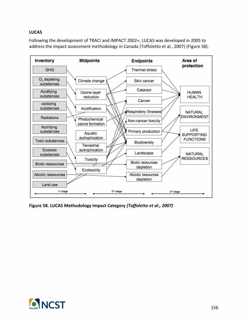
156

LUCAS

Following the development of TRACI and IMPACT 2002+, LUCAS was developed in 2005 to address the impact assessment methodology in Canada (Toffoletto et al., 2007) (Figure 58).

Figure 58. LUCAS Methodology Impact Category (Toffoletto et al., 2007)

157

ReCiPe

This method is a well-developed mythology encompassing both Eco-Indictor 99 and CML 2002 in terms of aggregation of both of the midpoint and endpoint assessment. The method is not published as a single document, but most impact categories have been described in peer reviewed publications (Goedkoop et al., 2009) (Figure 59).

Figure 59. ReCiPe Methodology Impact Category (Goedkoop et al., 2009)

158

EDIP97 and EDIP2003

EDIP2003 model, developed following the EDIP97, incorporates midpoint environmental impact assessment and normalization factors for regional information. This method includes exposure factors to different emissions regarding human toxicity, eco toxicity, photochemical ozone formation, and acidification (Hauschild and Potting, 2005). (Figure 60). See http://ipt.dtu.dk/~mic/EDIP97 and http://ipt.dtu.dk/~mic/EDIP2003.

Figure 60. EDIP Methodology Impact Category (Hauschild and Potting, 2005)

159

Annex C: CAL-B/C

Figure 61. CAL-B/C Components

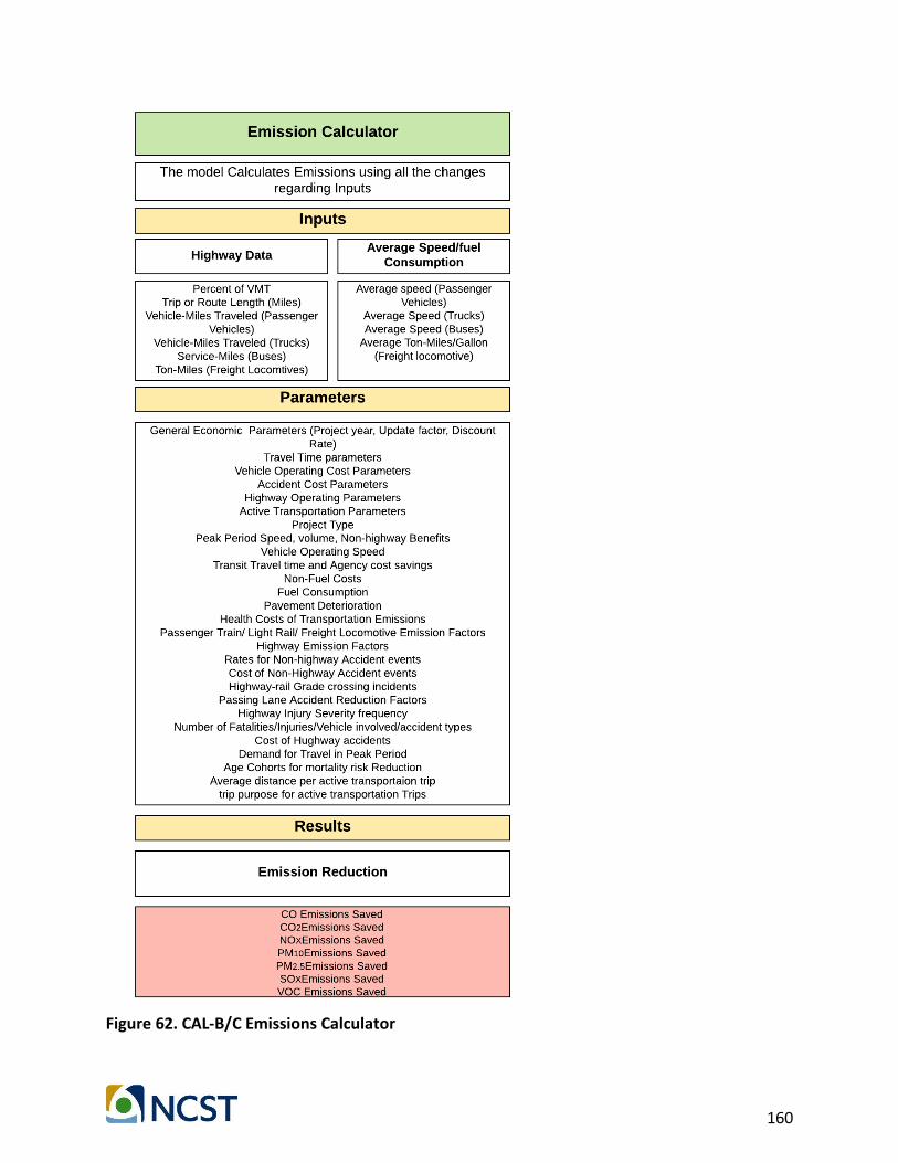
160

Figure 62. CAL-B/C Emissions Calculator