A

(lasdh©

K

1

ignplffcocmitit

l

0d

J. Non-Newtonian Fluid Mech. xxx (2006) xxx–xxx

Development and implementation of VOF-PROST for 3Dviscoelastic liquid–liquid simulations

D. Khismatullin b, Y. Renardy a,∗, M. Renardy a

a Department of Mathematics and ICAM, 460 McBryde Hall, Virginia Tech, Blacksburg, VA 24061-0123, USAb Department of Biomedical Engineering, 136 Hudson Hall, Box 90281, Duke University, Durham, NC 27708, USA

Received 15 February 2005; received in revised form 13 January 2006; accepted 21 February 2006

bstract

We implement a volume-of-fluid algorithm with a parabolic re-construction of the interface for the calculation of the surface tension forceVOF-PROST). This achieves higher accuracy for drop deformation simulations in comparison with existing VOF methods based on a piecewiseinear interface re-construction. The algorithm is formulated for the Giesekus constitutive law. The evolution of a drop suspended in a second liquidnd undergoing simple shear is simulated. Numerical results are first checked against two cases in the literature: the small deformation theory forecond-order liquids, and an Oldroyd-B extensional flow simulation. We then address the experimental data of Guido et al. (2003) for a Newtonianrop in a viscoelastic matrix liquid. The data deviate from existing theories as the capillary number increases, and reasons for this are explored

ere with the Oldroyd-B and Giesekus models.

2006 Elsevier B.V. All rights reserved.

ciftpiges[dweraia

eywords: Drop breakup; Oldroyd-B model; Volume-of-fluid method

. Introduction

Experimental photographs of a drop of viscous liquid shearedn another in Stokes flow are given in [1–7]. The study of a sin-le drop applies to dilute shear-mixing for which coalescence isegligible [8–13]. The volumes of daughter droplets depend onhysical properties and conditions of shear, and affect the rheo-ogical properties of the mixture [14–18]. In particular, the grosseatures of drop size distributions for the case of equal viscosityor Stokes flow have been simulated numerically with a VOFontinuous-surface-force (CSF) algorithm [19]. In the contextf drop breakup simulations, however, CSF leads to spuriousurrents and errors, which do not disappear with mesh refine-ent. Smoothing on a scale large relative to the mesh helps, but

s unrealistic in 3D simulations. Smoothing is not needed forhe more accurate calculation of interface curvature describedn Section 3, the ‘parabolic reconstruction of the interface for

he calculation of the surface tension force’ (PROST) [20].

In this paper, we focus on the development of a viscoelasticiquid–liquid PROST code. A number of experiments have been

∗ Corresponding author. Tel.: +1 540 320 1573; fax: +1 540 231 5960.E-mail address: renardyy@math.vt.edu(Y. Renardy).

i

shtat

377-0257/$ – see front matter © 2006 Elsevier B.V. All rights reserved.oi:10.1016/j.jnnfm.2006.02.013

onducted on the effect of elasticity on the deformation of a dropn a matrix fluid [6,21–23]. They have shown that elasticity af-ects the amount of drop deformation as well as the angle, whichhe drop makes with the flow direction. Results reported on ex-eriments in the literature vary in their conclusions. In [21,24],t is reported that viscoelasticity has a major effect on drop elon-ation, with drop elasticity suppressing deformation and matrixlasticity enhancing it. Numerical computations in [25] showimilar trends. On the other hand, recent work by Guido’s group6,26,27] shows that, at low capillary and Weissenberg numbers,rop extension is virtually unchanged by elasticity, in agreementith second order fluid theory, and the main effect of matrix

lasticity is to rotate the drop into the flow direction. Outside theange where second order theory is valid, the experiments actu-lly show a decrease in drop deformation when the matrix fluids elastic. Recent simulations by Yue et al. [28] also show suchdecrease at moderate Weissenberg number, while an increase

s found at higher Weissenberg number.We mention in passing that some experiments have also

hown new modes of breakup driven by normal stresses, which

ave no analog in the Newtonian case [29–32]. In these cases,he drop is elastic, and it stretches in the spanwise direction, likesausage being rolled. This process evolves much more slowly

han “ordinary” breakup and seems to be beyond the reach of

JNNFM-2601; No. of Pages 12

2 tonian

nct

eq

2

fllvη

η

w

T

F

wtc

Tt

C

j∇f

2

lTs

γ

iyf

0iidaeut

2

tL

ps

lfltacict

2

oa

ciaβ

3

aaavp

Taa

co

3

D. Khismatullin et al. / J. Non-New

umerical simulations at this point. This effect should not beonfused with the minor drop widening in the spanwise direc-ion that is observed in some Newtonian flows [33].

Our computations will focus on the range of parameters cov-red in the Guido experiments [26]. The results show trendsualitatively consistent with the experiments.

. Governing equations

We consider shearing flow of a drop surrounded by a matrixuid. Both liquids are modeled by the Giesekus model. The two

iquids may differ in density ρ, solvent viscosity ηs, polymericiscosity ηp, and relaxation time λ. The total viscosity is denoted= ηs + ηp, and the elastic modulus at time 0 is denoted G(0) =

p/λ.The governing equations for the VOF approach are:

∇ · u = 0,

ρ

(∂u∂t

+ u · ∇u)

= ∇ · T − ∇p

+∇ · (ηs(∇u + (∇u)T )) + F, (1)

here T is the extra stress tensor.The total stress tensor is τ = −pI + T + ηs[∇u + (∇u)T ].

he body force is equal to the interfacial tension force:

= σκ̃nδs, (2)

here σ denotes the surface tension coefficient, n the normalo the interface, δs the δ-function at the interface, and κ̃ theurvature −∇ · n. [34].

The constitutive equation for the Giesekus model is:

λ

(∂T∂t

+ (u · ∇)T − (∇u)T − T(∇u)T)

+ T + λκT2

= λG(0)(∇u + (∇u)T ). (3)

he interface is represented as the surface where a color func-ion:

(x, t) ={

0 in the matrix liquid

1 in the drop(4)

umps in value. C is advected by the flowfield. In F, n =C/|∇C|, δs = |∇C|. The numerical implementation of the sur-

ace tension force will be described later.

.1. Boundary conditions

The drop is initially spherical with radius a. The walls areocated at z = 0, Lz, and move horizontally with speeds ±U0.he boundary conditions at the upper and lower walls impose ahear rate of:

˙ = U ′(z) = 2U0 (5)

Lz

n the matrix liquid. Spatial periodicity is imposed in the x anddirections. Additional boundary conditions are not needed

or the extra stress components. The computational domain

tit

Fluid Mech. xxx (2006) xxx–xxx

≤ x ≤ Lx, 0 ≤ y ≤ Ly, 0 ≤ z ≤ Lz is chosen so that we min-mize the effect neighboring drops and that of the walls. Typ-cally, the distance between the walls is eight times the dropiameter, the spanwise period is four times the drop diameter,nd the period in the flow direction is chosen dependent on dropxtension. We have found, in these and prior (Newtonian) sim-lations, that the influence of the boundaries is negligible underhese circumstances.

.2. Initial conditions

The initial flow field is simple shear for both the drop andhe matrix fluids. This is (U(z), 0), satisfying U(z) = U0(2z −z)/Lz. The stresses are set equal to the values which wouldrevail in the corresponding steady shear flow with the givenhear rate.

This initial condition, used in most of the computations be-ow, corresponds to a drop being placed into a pre-existing shearow. Alternatively, we can consider a shear flow started up with

he drop in place; the difference is that the viscoelastic stressesre initially zero. We shall see some differences between the twoases, as discussed in Section 4.1 below. Even in these compar-sons, we took the initial velocity field to be linear and did notonsider any transient propagation of shear waves starting fromhe walls.

.3. Parameters

The dimensionless parameters are the viscosity ratio (basedn total viscosities) m = ηdrop/ηmatrix, a capillary number Ca =γ̇ηmatrix/σ which measures the competition between the vis-ous force causing deformation versus capillary force keep-ng the drop together, a Reynolds number Re = ργ̇a2/ηmatrix,

Weissenberg number We = γ̇λ and retardation parameter= ηs/η.

. Viscoelastic PROST algorithm

A rectangular Cartesian staggered mesh is used. Fig. 1 showstypical staggered grid cell on which the unknowns are evalu-

ted at different locations as indicated. The u-velocity is centeredt the back face, the v-velocity at the left side face, and the w-elocity is centered at the bottom face of the cell. The pressurei,j,k and the color function C(i, j, k) are located at the center.he diagonal components of the extra stress tensor take valuest the center of the cell, while each off-diagonal component ist the mid-point of an edge.

There are two primary features to the solution method: the cal-ulation of the interfacial tension force and the time-integrationf the governing equations.

.1. Calculation of the interfacial tension force

The body force for a grid cell cut by the interface includeshe interfacial tension force. When such an interface cell shownn Fig. 2 is encountered in PROST (parabolic reconstruction ofhe surface tension force), a quadratic surface is fitted through

D. Khismatullin et al. / J. Non-Newtonian Fluid Mech. xxx (2006) xxx–xxx 3

riable

ir

k

wnTtaciatgTtasF

3

mi[bgm

tlftfi

Tf

Fig. 1. Location of va

t plus neighboring cells, totalling 27 cells in 3D. The surface isepresented by

+ n · (x − x0) + (x − x0) · A(x − x0) = 0, (6)

here k is a constant, x0 the center of the interface cell, n the unitormal, and A the 3 × 3 real symmetric matrix such that An = 0.he equation of the interface involves six parameters, one in k,

wo in n and three in A (in view of the constraint An = 0), whichre determined by a weighted least square fit to the values of theolor function in the interface cell and its 26 neighbors. After thenterface has been found, the curvature is calculated as κ̃ = 2tr A,nd the surface tension force is calculated as F = −σκ̃∇C. Herehe discretization for ∇C is the same as that of the pressureradient, so that exact cancellation is possible if κ̃ is constant.his allows a sphere to be an exact equilibrium shape even for

he discretized problem and avoids the parasitic currents whichppear with more traditional discretizations such as continuousurface force (CSF) or continuous surface stress (CSS) [34–37].or further details we refer to [20].

.2. Semi-implicit time-integration of governing equations

A semi-implicit time-integration scheme with a projectionethod was devised in [19,38] to treat the momentum equation

n the Newtonian case. This was further modified for PROST

20] where we note that the body force F = (F1, F2, F3) is giveny the singular surface tension force and the p includes the sin-ular pressure which is needed to balance it. We choose p1 toake (F − ∇p1) divergence free; this then appears in place of

=vig

Fig. 2. PROST fits a quadratic surface through the inte

s in a MAC mesh cell

he body force in the projected equation for the intermediate ve-ocity field u∗ = (u∗, v∗, w∗). Next, a Poisson equation is solvedor the remainder of p, denoted p2. To exemplify this procedure,ake for instance the x-component of the intermediate velocityeld after the nth timestep:

u∗ − un

�t= −(un · ∇)un + 1

ρ

(Fn

1 − ∂p1

∂x

)

+ 1

ρ

(∂T n

11

∂x+ ∂T n

12

∂y+ ∂T n

13

∂z

)+ 1

ρ

∂

∂x

(2ηs

∂u∗

∂x

)

+ 1

ρ

∂

∂y

(ηs

∂u∗

∂y+ ηs

∂vn

∂x

)

+ 1

ρ

∂

∂z

(ηs

∂u∗

∂z+ ηs

∂wn

∂x

). (7)

he Stokes operator terms for u∗ are treated implicitly and theyactorize:

(I − �t

ρ

∂

∂x

(2ηs

∂

∂x

)) (I − �t

ρ

∂

∂y

(ηs

∂

∂y

))

×(

I − �t

ρ

∂

∂z

(ηs

∂

∂z

))u∗ (8)

explicit terms. The solution of this step is accomplished by in-erting tridiagonal matrices. The v∗ and w∗ components of thentermediate velocity field are computed analogously. The diver-ence free condition for the velocity yields a Poisson equation

rface cell with center x0 plus neighboring cells.

4 tonian

f

∇

T

Tcn

t

w

sc

Twti

tMvsiettt

TtbWai

tps

cG

imasc

w

λ

F

λ

PlsOTie

nfsltNocitmlTm

λ

W

φ

I ( )

D. Khismatullin et al. / J. Non-New

or pressure:

·(∇p2

ρ

)= −∇ · u∗

�t. (9)

he velocity field for the (n + 1)th timestep is found from:

un+1 − u∗

�t= −∇p2

ρ.

his equation also provides a homogeneous Neumann boundaryondition for the determination of p2, since the normal compo-ent of un+1 is required to vanish on the boundary.

The constitutive equations are discretized by treating the spa-ial derivative terms for the extra stress tensor implicitly. Thus:

λ

(Tn+1 − Tn

�t+

(un ∂

∂x+ vn ∂

∂y+ wn ∂

∂z

)Tn+1

)

+ Tn+1 + λκ(Tn)2

= λ((∇un)Tn + Tn(∇u)nT + G(0)(∇un + (∇u)nT )),

(10)

here (∇u)ij = ∂ui

∂xj. The solution of each component of the extra

tress tensor is decoupled. Next, the operator on Tn+1 factorizesonveniently with an error of O((�t)2):

(λ + �t)

(1 + λ

λ + �tun�t

∂

∂x

) (1 + λ

λ + �tvn�t

∂

∂y

)

×(

1 + λ

λ + �twn�t

∂

∂z

)Tn+1 = explicit terms. (11)

his leads to inversions of tridiagonal matrices, and speeds uphat would have been a large matrix inversion. This approach to

he discretization of the constitutive equations parallels the semi-mplicit time integration for the momentum equation [38,19,37].

We preserve the positive definite property of the extra stressensor in our algorithm. The time-dependent upper-convected

axwell constitutive equations have an instability if an eigen-alue of the extra stress tensor T is less than −G(0) [39]. It washown later that this would not happen if the initial conditions physically realistic. However, this could happen numerically;.g., in a grid cell traversed by an interface separating a New-onian liquid and a viscoelastic one. Note that the properties ofhe fluid in the cell are interpolated from the properties of thewo liquids:

λ = Cλ1 + (1 − C)λ2, ρ = Cρ1 + (1 − C)ρ2,

ηs = Cηs1 + (1 − C)ηs2, ηp = Cηp1 + (1 − C)ηp2, (12)

his results in a ‘partly elastic liquid’ which changes proper-ies as the interface moves, and may end up violating the sta-ility constraint. Indeed, we observe this at moderate to higheissenberg numbers. We correct this numerical instability by

dding a multiple of the identity matrix to T over interface cellsf an eigenvalue is less than −G(0).

Specifically, we interpolate the off-diagonal components ofhe stress linearly to the cell centers, so we have all stress com-onents defined there. We then compute the eigenvalues of thetress, and correct them if positive definiteness is violated. If the

φ

wa

Fluid Mech. xxx (2006) xxx–xxx

ell is an interface cell, the fluid properties required to compute(0) are interpolated according to Eq. (12).We note that this method of enforcing positive definiteness

s rather ad hoc, and questions about its impact on accuracyight arise. To assess this issue, we developed a more systematic

pproach. Numerical tests revealed no significant difference. Forimplicity, we shall give the following discussion for the specialase of the Oldroyd B model.

In the constitutive equation:

λ

(∂T∂t

+ (u · ∇)T − (∇u)T − T(∇u)T)

+ T

= λG(0)(∇u + (∇u)T ), (13)

e set S = T + G(0)I. We then find:(∂S∂t

+ (u · ∇)S − (∇u)S − S(∇u)T)

+ T = 0. (14)

rom the latter equation, we derive that:[∂

∂t+ (u · ∇)

]ln detS + tr(S−1T) = 0. (15)

ositive definiteness can now be enforced by keeping track ofn detS as a separate variable in the code. It is updated by theame algorithm described for the viscoelastic stresses above.nce we have a value of φ = ln detS and hence detS, we adjustby a multiple of the identity in such a fashion that T + G(0)I

s positive definite and its determinant has the prescribed valuexp(φ).

Some care needs to be taken to make this approach work. Weote that, in the interest of keeping all computations on a uni-orm grid, our algorithm assigns a “viscoelastic stress” (whichhould be zero) even to the Newtonian phase. We have a prob-em defining S−1 if one of the fluids is Newtonian. To get aroundhis, we actually put a small viscoelastic modulus even into theewtonian phase (in practice we chose a ratio of 10−4). An-ther issue is that a moderate change in ln detS causes a largehange in detS. Moreover, our use of a staggered grid requiresnterpolation of stress components between nodes. Near the in-erface, where the viscoelastic modulus can jump by orders of

agnitude, this can cause T + G(0)I to become almost singu-ar, resulting in certain components of S−1T becoming large.his will cause the code to blow up. To deal with this issue, weodify the discretization of (15):[φn+1 − φn

�t+ (u · ∇)φn+1

]+ tr((Sn)−1Tn) = 0. (16)

e can put this in the form:

n+1 + �t(u · ∇)φn+1 = φn − �t

λtr((Sn)−1Tn). (17)

n this last equation, we now replace the right hand side by

n + ln 1 − �t

λtr((Sn)−1Tn) , (18)

hich is formally equivalent up to an error of order (�t)2, butvoids the blowup at the interface.

tonian

4

4

N

wftN

Narop

D

wtl

D

wdcseit

s

Fdff

D. Khismatullin et al. / J. Non-New

. Numerical results

.1. Small deformation

The ratio of elastic stress to interfacial stress is:

= �1γ̇2a

2σ, (19)

here �1 is the first normal stress coefficient. In the small de-ormation limit, non-Newtonian effects appear during deforma-ion when N is comparable to Ca2 [40]. The higher the ratio/Ca2, the more different the drop evolution would be from theewtonian counterpart. Ref. [40] used the second-order fluid

pproximation with small Ca and N, and N/Ca2 = O(1), to de-ive asymptotic expansions for the angle φmax of the major axis

f the approximate ellipsoid with the x-axis. The deformationarameter is:

= (Rmax − Rmin)

(Rmax + Rmin), (20)

lTTa

ig. 3. C1–D2 fluid pair at Ca = 0.05, Re = 0.07, m = 0.1, Wematrix = 0.23, β = 0enote small deformation theory (21) for Newtonian and viscoelastic matrix liquidsrom the simulation. The ellipse of best fit is drawn through them. One line goes throuarthest away from the center of the drop. (c) Error of the elliptical fit as a function of

Fluid Mech. xxx (2006) xxx–xxx 5

here Rmax and Rmin denote the maximum and minimum dis-ances of the interface from the drop center, respectively. Ateading order:

= Ca T

2, φmax = π

4+ Ca

T

(s4 + N

Ca2 g4

), (21)

here T = (16 + 19m)/[8(1 + m)]. The terms s4 and g4 alsoepend on m, but not on N. Thus, the effect of elasticity is tohange φmax from the Newtonian case, while D remains theame. The constancy of D reflects the cancellation of two effects:lastic stresses pulling on the drop and the rotation of the dropnto the flow direction, which decreases the total shear to whichhe drop is subjected.

The experimental study of [26] correlates well with (21) atmall capillary numbers. We perform direct numerical simu-

ations for one of their fluid pairs, named C1–D2, at 20 ◦C.he drop liquid D2 is a silicone oil with viscosity 1.12 Pa s.he viscoelastic matrix liquid C1 has total viscosity 10.3 Pa s,first normal stress difference coefficient �1 = 7.5 Pa s2, and

.127. (a) Evolution of D and φmax; t is in units of γ̇−1. The states ‘+’ and ‘o’, respectively. (b) x–z cross-section of stationary state. Dots denotes raw datagh its major axis, and another joins the drop center to the node on the interfaceangle with the horizontal. A positive error indicates points outside the ellipse.

6 D. Khismatullin et al. / J. Non-Newtonian Fluid Mech. xxx (2006) xxx–xxx

F0zV

N

T

λ

Is0

wc

F(sNi

Fso

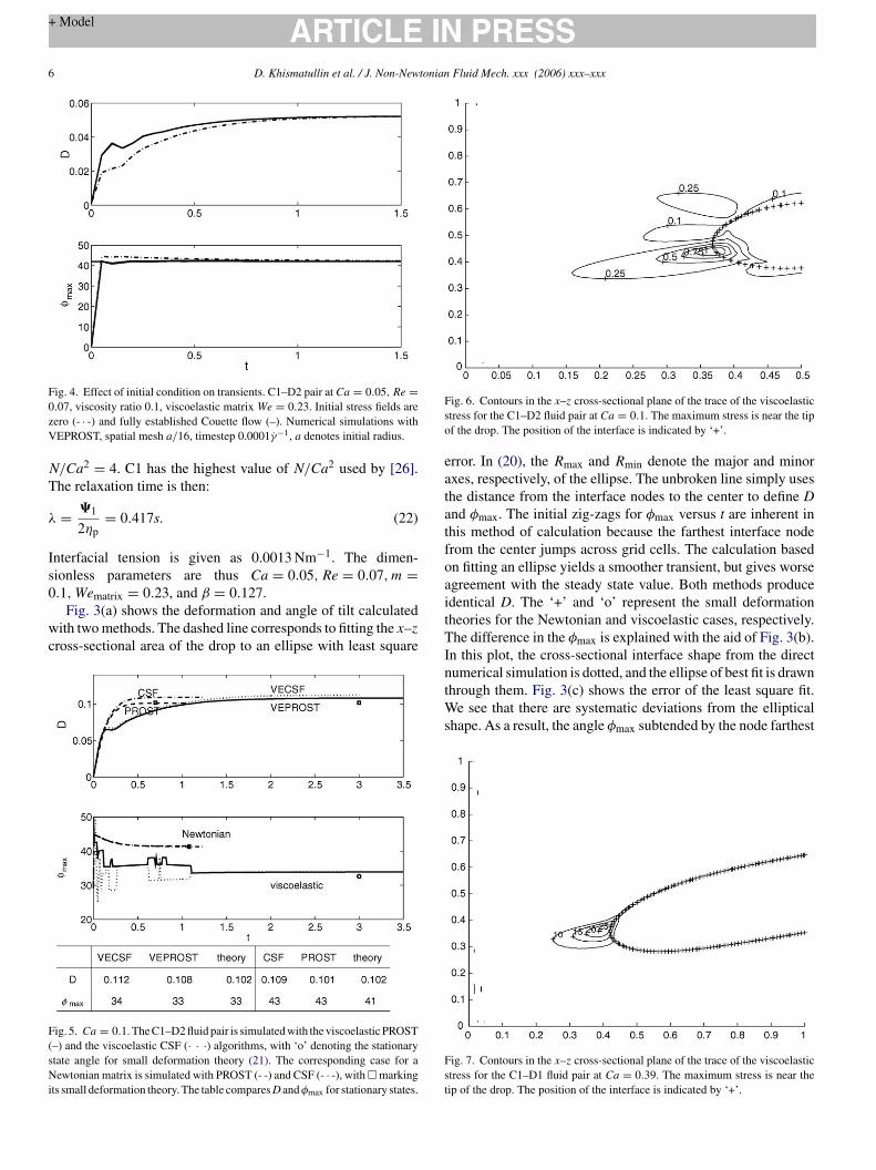
eatatfoa

ig. 4. Effect of initial condition on transients. C1–D2 pair at Ca = 0.05, Re =.07, viscosity ratio 0.1, viscoelastic matrix We = 0.23. Initial stress fields areero (- · -) and fully established Couette flow (–). Numerical simulations withEPROST, spatial mesh a/16, timestep 0.0001γ̇−1, a denotes initial radius.

/Ca2 = 4. C1 has the highest value of N/Ca2 used by [26].he relaxation time is then:

= �1

2ηp= 0.417s. (22)

nterfacial tension is given as 0.0013 Nm−1. The dimen-ionless parameters are thus Ca = 0.05, Re = 0.07, m =

.1, Wematrix = 0.23, and β = 0.127.

Fig. 3(a) shows the deformation and angle of tilt calculatedith two methods. The dashed line corresponds to fitting the x–z

ross-sectional area of the drop to an ellipse with least square

ig. 5. Ca = 0.1. The C1–D2 fluid pair is simulated with the viscoelastic PROST–) and the viscoelastic CSF (· · ·) algorithms, with ‘o’ denoting the stationarytate angle for small deformation theory (21). The corresponding case for aewtonian matrix is simulated with PROST (- -) and CSF (- · -), with � marking

ts small deformation theory. The table compares D andφmax for stationary states.

itTIntWs

Fst

ig. 6. Contours in the x–z cross-sectional plane of the trace of the viscoelastictress for the C1–D2 fluid pair at Ca = 0.1. The maximum stress is near the tipf the drop. The position of the interface is indicated by ‘+’.

rror. In (20), the Rmax and Rmin denote the major and minorxes, respectively, of the ellipse. The unbroken line simply useshe distance from the interface nodes to the center to define Dnd φmax. The initial zig-zags for φmax versus t are inherent inhis method of calculation because the farthest interface noderom the center jumps across grid cells. The calculation basedn fitting an ellipse yields a smoother transient, but gives worsegreement with the steady state value. Both methods producedentical D. The ‘+’ and ‘o’ represent the small deformationheories for the Newtonian and viscoelastic cases, respectively.he difference in the φmax is explained with the aid of Fig. 3(b).

n this plot, the cross-sectional interface shape from the direct

umerical simulation is dotted, and the ellipse of best fit is drawnhrough them. Fig. 3(c) shows the error of the least square fit.

e see that there are systematic deviations from the ellipticalhape. As a result, the angle φmax subtended by the node farthest

ig. 7. Contours in the x–z cross-sectional plane of the trace of the viscoelastictress for the C1–D1 fluid pair at Ca = 0.39. The maximum stress is near theip of the drop. The position of the interface is indicated by ‘+’.

D. Khismatullin et al. / J. Non-Newtonian Fluid Mech. xxx (2006) xxx–xxx 7

Fsκ

i

fabao[

tstoz

tt(s

F(

F(w

Pwfista

sstC

5In Fig. 6, we show a plot of the viscoelastic stresses for the

C1–D2 pair at Ca = 0.1. The graph shows a contour plot of

ig. 8. Contours in the x–z cross-sectional plane of the trace of the viscoelastictress for the C1–D1 fluid pair at Ca = 0.39 and with a Giesekus parameter of= 0.1. The maximum stress is near the tip of the drop. The position of the

nterface is indicated by ‘+’.

rom the drop center differs from the ellipsoidal theory by 2◦,s reflected in Fig. 3(a). The stationary states in Fig. 3 haveeen checked to be independent of mesh size and timestep sizet �x = �y = �z = a/16, �t = 0.0005γ̇−1, and the influencef the boundaries is negligible with a computational domain0, 16a] × [0, 8a] × [0, 8a].

The evolution of the initial transient is sensitive to the ini-ial stress distribution. Fig. 4 compares two different initialtress fields. The line represents starting the simulation fromhe stresses of a fully established Couette flow. This leads to anvershoot that is not present when the simulation begins withero stresses.

Fig. 5 shows Ca = 0.1 with VEPROST (–) and the viscoelas-

ic CSF code described in [41] (· · ·). The analogous New-onian fluid system is simulated with PROST (- -) and CSF- ·).We see that the Newtonian system reaches the stationarytate (�), much earlier than the viscoelastic system (©). VE-

ig. 9. C1–D1 fluid pair at Ca = 0.16. The experimental data of Guido et al.- · -) is compared with numerical results with VEPROST (—) with β = 0.5.

t

FsBs0

ig. 10. C1–D1 fluid pair at Ca = 0.33. The experimental data of Guido et al.- · -) is compared with numerical results with VEPROST with β = 0.5 (- -) andith the additional Giesekus parameter κ2 = 0.1 (—).

ROST performs slightly better than VECSF in comparisonith the small deformation theory. Spatial and temporal re-nements were performed until D and φmax are converged toeveral digits: for this figure, this is achieved for a computa-ional domain [0, 16a] × [0, 8a] × [0, 8a], �x = �y = �z =/16, and �t = 0.0002γ̇−1.

Table 1 shows that the small deformation theory is a rea-onable approximation for this range of capillary number. Formall deformation, the final state is independent of the split ofhe total viscosity into solvent and polymer viscosities; e.g., ata = 0.14, numerical simulations for the cases ηs = 1.3 and.15 for total viscosity 10.3 evolve to the same D.

he trace of the viscoelastic stress tensor. We see a strong stress

ig. 11. C1–D1 fluid pair at Ca = 0.39. Evolution of deformation during tran-ient motion: experimental data of [26] (©), numerical results using Oldroyd-

model with β = 0.5 (�), Newtonian counterpart (�), Newtonian with 10%hear-thinning in the matrix liquid (- -), Giesekus model with κ = 0.1 (�) and.2 (- · -).

8 D. Khismatullin et al. / J. Non-Newtonian Fluid Mech. xxx (2006) xxx–xxx

Fig. 12. C1–D1 at Ca = 0.39. Evolution to stationary state: experimental data of[26] (©), Newtonian with 10% shear-thinning in the matrix liquid (- -), Giesekusmodel with κ = 0.1 (�) and 0.2 (-.-).

Table 1Viscoelastic PROST code is used to calculate stationary states

Ca D Dsdt %�D φ0max φmax,sdt %�φmax

0.05 0.052 0.051 2% 39.9 38.8 3%0.1 0.108 0.102 6% 33.9 32.6 4%

R%

msiotNi

pm

Fig. 13. C1–D1 fluid pair at Ca = 0.39. (a) β = 0.005 (- · -); β = 0.5 (· · ·); β = 0�t = 0.0005γ̇−1. (b) Velocity vector field in vertical cross-section of the drop in statifor C1–D1 pair, β = 0.5, D = 0.5, φmax = 16◦.

0.14 0.160 0.142 12.6% 28.7 27.7 4%

esults are compared with small deformation theory (sdt) for C1–D2 pair;�D = |D − Dsdt|100/Dsdt, %�φmax = |φmax − φmax,sdt|100/φmax,sdt.

aximum near the tip of the drop and a secondary maximum,eparated by a low stress region. Similar trends were observedn the 2D simulations of [41]. The largest elastic stress devel-ps right at the interface. It is inherent in the method used herehat there is some spreading of “viscoelastic” stresses into theewtonian phase, and the mesh used (1/12 of the drop radius)

s relatively coarse.Figs. 7 and 8 show analogous stress plots for the C1–D1 fluid

air at Ca = 0.39 with the Oldroyd B model and with a Giesekusodel using κ = 0.1. In both cases we see a pronounced stress

.91 (- -); Newtonian system (–). Mesh size �x = �y = �z = a/8, time steponary state for the Newtonian counterpart problem, D = 0.58, φmax = 14◦; (c)

tonian Fluid Mech. xxx (2006) xxx–xxx 9

mnm

4

Biφ

fφ

tiusTs[stm0s

nfidO(etd

fBNGa�

timiκ

sti

faoT1

pi

Fig. 14. Newtonian drop in a viscoelastic liquid with We = 0.4, Ca = 0.24.Re = 0.03, ηs/ηp = 1, equal viscosity. The plots show Ca = 0.24 and 0.6. Thedashed line is for a Newtonian matrix at Ca = 0.6. Computational mesh a/16,timestep 0.0005γ̇−1, a is the drop radius.

D. Khismatullin et al. / J. Non-New

aximum near the tip of the drop; due to the shear-thinningature of the model, the stresses for the Giesekus model areuch smaller.

.2. Large deformation

The shear rate is increased to achieve larger deformations.oth Ca and We increase linearly with shear rate. The exper-

mentally observed stationary states in [26] then have largermax and smaller D than the values predicted by the small de-ormation theory (21). Data on the time-dependence of D andmax for large deformation were provided to the authors for

he C1–D1 fluid pair at 25 ◦C. The drop liquid D1 is a sil-cone oil with viscosity 6.6 Pa s. The viscoelastic matrix liq-id C1 at 25 ◦C has total viscosity 6.6 Pa s, a first normaltress difference coefficient �1 = 3.5 Pa s2, and N/Ca2 = 0.6.he interfacial tension is 0.0013 N/m. The experimentally mea-ured φmax for the stationary states are plotted in Fig. 5 of26]. Our first data set concerns Ca = 0.16 which is just out-ide of the range of small deformation theory. Fig. 9 showshat the experimental data (- · -) compare well with our nu-

erical results (—) obtained at �x = �y = �z = a/8, �t =.0001, Lx = 16a, Ly = Lz = 8a, ηs = ηp = 3.3. The dimen-ionless relaxation time or Weissenberg number is We = 0.24.

When shear rate is increased, it is clear that the matrix liquid isot as well-described by the Oldroyd-B model as in the previousgure. For example, Fig. 10 is a comparison of the experimentalata (- · -) at Ca = 0.33 with our numerical results obtained theldroyd-B model (- -) and the Giesekus model with κ2 = 0.1

—). The Oldroyd-B model predicts more extension than thexperimental data, while a small amount of shear-thinning inhe matrix liquid, modeled with κ2 = 0.1, provides a good pre-iction.

Fig. 11 compares the evolution of deformation at Ca = 0.39or the experimental data (©) with simulations for the Oldroyd-

model with β = 0.5 (�), the Newtonian counterpart (�),ewtonian with 10% shear-thinning in the matrix liquid (- -),iesekus model with κ = 0.1 (�), and 0.2 (- · -). Tests with mesh

nd timestep refinements were also conducted around mesh sizex = �y = �z = a/12, �t = 0.0001γ̇−1. We conclude that

he discrepancy between the numerical and experimental datan the transient zone is associated with shear-thinning of the

atrix liquid. A closer view of the evolution to stationary states shown in Fig. 12. The Newtonian 10% shear-thinned case and= 0.1 case are close and in good approximation over the tran-

ient evolution. On the other hand, there is a slight retraction ofhe experimentally observed drop over a much longer time thats not captured by these models.

Fig. 13 shows that the numerical results on a rough meshor D and φmax are not sensitive to changes in β, and in factre close to the Newtonian system. This implies that the valuef N/Ca2 = 0.6 corresponds to a small influence of elasticity.here are minor differences in the flow field as shown in Fig.

3(b) and (c).

We mention that a level-set method is used in [25] to com-ute the deformation of a circular interface in 2D and spher-cal in 3D with the Oldroyd B model. Their 2D results at

Fig. 15. Newtonian drop in a viscoelastic liquid. Velocity field in a cross-sectionin the x–z plane for the stationary state. Re = 0.03, ηs/ηs = 1, equal viscos-ity, We = 0.4, Ca = 0.24. Computational box 16a cube, mesh a/16, timestep0.0005γ̇−1.

1 tonian

R

wD

1c(tts

C

et

sFRsti

nd

Fmd

0 D. Khismatullin et al. / J. Non-New

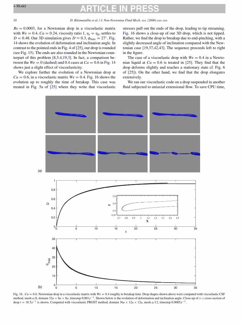
e = 0.0003, for a Newtonian drop in a viscoelastic matrixith We = 0.4, Ca = 0.24, viscosity ratio 1, ηs = ηp, settles to= 0.48. Our 3D simulation gives D ≈ 0.3, φmax = 27◦. Fig.

4 shows the evolution of deformation and inclination angle. Inontrast to the pointed ends in Fig. 4 of [25], our drop is roundedsee Fig. 15). The ends are also rounded in the Newtonian coun-erpart of this problem [8,5,4,19,3]. In fact, a comparison be-ween the We = 0 (dashed) and 0.4 cases at Ca = 0.6 in Fig. 14hows just a slight effect of viscoelasticity.

We explore further the evolution of a Newtonian drop ata = 0.6, in a viscoelastic matrix We = 0.4. Fig. 16 shows the

volution up to roughly the time of breakup. This case wasreated in Fig. 5a of [25] where they write that viscoelastic

oe

fl

ig. 16. Ca = 0.6. Newtonian drop in a viscoelastic matrix with We = 0.4 roughly toethod, mesh a/8, domain 32a × 8a × 8a, timestep 0.001γ̇−1. Shown below is the e

rop t = 18.5γ̇−1 is shown. Computed with viscoelastic PROST method, domain 36

Fluid Mech. xxx (2006) xxx–xxx

tresses pull out the ends of the drop, leading to tip streaming.ig. 16 shows a close-up of our 3D drop, which is not tipped.ather, we find the drop to breakup due to end-pinching, with a

lightly decreased angle of inclination compared with the New-onian case [19,37,42,43]. The sequence proceeds left to rightn the figure.

The case of a viscoelastic drop with We = 0.4 in a Newto-ian liquid at Ca = 0.6 is treated in [25]. They find that therop deforms slightly and reaches a stationary state cf. Fig. 6

f [25]). On the other hand, we find that the drop elongatesxtensively.

We ran our viscoelastic code on a drop suspended in anotheruid subjected to uniaxial extensional flow. To save CPU time,

breakup time. Drop shapes shown above were computed with viscoelastic CSFvolution of deformation and inclination angle. Close-up of x–z cross-section ofa × 12a × 12a, mesh a/12, timestep 0.0005γ̇−1.

D. Khismatullin et al. / J. Non-Newtonian Fluid Mech. xxx (2006) xxx–xxx 11

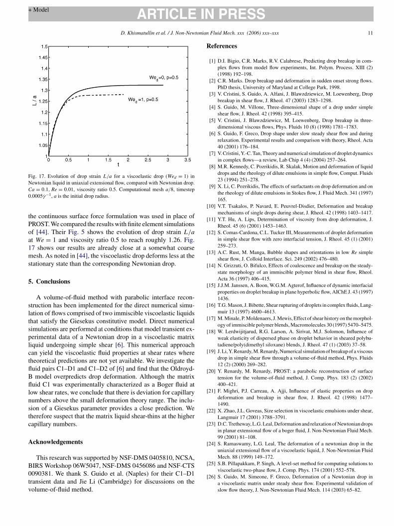
Fig. 17. Evolution of drop strain L/a for a viscoelastic drop (Wed = 1) inNC

0

tPoa1ms

5

sltsplctflBfllnstc

A

B0tv

References

[1] D.I. Bigio, C.R. Marks, R.V. Calabrese, Predicting drop breakup in com-plex flows from model flow experiments, Int. Polym. Process. XIII (2)(1998) 192–198.

[2] C.R. Marks. Drop breakup and deformation in sudden onset strong flows.PhD thesis, University of Maryland at College Park, 1998.

[3] V. Cristini, S. Guido, A. Alfani, J. Blawzdziewicz, M. Loewenberg, Dropbreakup in shear flow, J. Rheol. 47 (2003) 1283–1298.

[4] S. Guido, M. Villone, Three-dimensional shape of a drop under simpleshear flow, J. Rheol. 42 (1998) 395–415.

[5] V. Cristini, J. Blawzdziewicz, M. Loewenberg, Drop breakup in three-dimensional viscous flows, Phys. Fluids 10 (8) (1998) 1781–1783.

[6] S. Guido, F. Greco, Drop shape under slow steady shear flow and duringrelaxation. Experimental results and comparison with theory, Rheol. Acta40 (2001) 176–184.

[7] V. Cristini, Y.-C. Tan, Theory and numerical simulation of droplet dynamicsin complex flows—a review, Lab Chip 4 (4) (2004) 257–264.

[8] M.R. Kennedy, C. Pozrikidis, R. Skalak, Motion and deformation of liquiddrops and the rheology of dilute emulsions in simple flow, Comput. Fluids23 (1994) 251–278.

[9] X. Li, C. Pozrikidis, The effects of surfactants on drop deformation and onthe rheology of dilute emulsions in Stokes flow, J. Fluid Mech. 341 (1997)165.

[10] V.T. Tsakalos, P. Navard, E. Peuvrel-Disdier, Deformation and breakupmechanisms of single drops during shear, J. Rheol. 42 (1998) 1403–1417.

[11] Y.T. Hu, A. Lips, Determination of viscosity from drop deformation, J.Rheol. 45 (6) (2001) 1453–1463.

[12] S. Comas-Cardona, C.L. Tucker III, Measurements of droplet deformationin simple shear flow with zero interfacial tension, J. Rheol. 45 (1) (2001)259–273.

[13] A.C. Rust, M. Manga, Bubble shapes and orientations in low Re simpleshear flow, J. Colloid Interface. Sci. 249 (2002) 476–480.

[14] N. Grizzuti, O. Bifulco, Effects of coalescence and breakup on the steady-state morphology of an immiscible polymer blend in shear flow, Rheol.Acta 36 (1997) 406–415.

[15] J.J.M. Janssen, A. Boon, W.G.M. Agterof, Influence of dynamic interfacialproperties on droplet breakup in plane hyperbolic flow, AIChE J. 43 (1997)1436.

[16] T.G. Mason, J. Bibette, Shear rupturing of droplets in complex fluids, Lang-muir 13 (1997) 4600–4613.

[17] M. Minale, P. Moldenaers, J. Mewis, Effect of shear history on the morphol-ogy of immiscible polymer blends, Macromolecules 30 (1997) 5470–5475.

[18] W. Lerdwijitjarud, R.G. Larson, A. Sirivat, M.J. Solomon, Influence ofweak elasticity of dispersed phase on droplet behavior in sheared polybu-tadiene/poly(dimethyl siloxane) blends, J. Rheol. 47 (1) (2003) 37–58.

[19] J. Li, Y. Renardy, M. Renardy, Numerical simulation of breakup of a viscousdrop in simple shear flow through a volume-of-fluid method, Phys. Fluids12 (2) (2000) 269–282.

[20] Y. Renardy, M. Renardy, PROST: a parabolic reconstruction of surfacetension for the volume-of-fluid method, J. Comp. Phys. 183 (2) (2002)400–421.

[21] F. Mighri, P.J. Carreau, A. Ajji, Influence of elastic properties on dropdeformation and breakup in shear flow, J. Rheol. 42 (1998) 1477–1490.

[22] X. Zhao, J.L. Goveas, Size selection in viscoelastic emulsions under shear,Langmuir 17 (2001) 3788–3791.

[23] D.C. Tretheway, L.G. Leal, Deformation and relaxation of Newtonian dropsin planar extensional flow of a boger fluid, J. Non-Newtonian Fluid Mech.99 (2001) 81–108.

[24] S. Ramaswamy, L.G. Leal, The deformation of a newtonian drop in theuniaxial extensional flow of a viscoelastic liquid, J. Non-Newtonian FluidMech. 88 (1999) 149–172.

[25] S.B. Pillapakkam, P. Singh, A level-set method for computing solutions to

ewtonian liquid in uniaxial extensional flow, compared with Newtonian drop.a = 0.1, Re = 0.01, viscosity ratio 0.5. Computational mesh a/8, timestep.0005γ̇−1, a is the initial drop radius.

he continuous surface force formulation was used in place ofROST. We compared the results with finite element simulationsf [44]. Their Fig. 5 shows the evolution of drop strain L/a

t We = 1 and viscosity ratio 0.5 to reach roughly 1.26. Fig.7 shows our results are already close at a somewhat coarseesh. As noted in [44], the viscoelastic drop deforms less at the

tationary state than the corresponding Newtonian drop.

. Conclusions

A volume-of-fluid method with parabolic interface recon-truction has been implemented for the direct numerical simu-ation of flows comprised of two immiscible viscoelastic liquidshat satisfy the Giesekus constitutive model. Direct numericalimulations are performed at conditions that model transient ex-erimental data of a Newtonian drop in a viscoelastic matrixiquid undergoing simple shear [6]. This numerical approachan yield the viscoelastic fluid properties at shear rates whereheoretical predictions are not yet available. We investigate theuid pairs C1–D1 and C1–D2 of [6] and find that the Oldroyd-model overpredicts drop deformation. Although the matrix

uid C1 was experimentally characterized as a Boger fluid atow shear rates, we conclude that there is deviation for capillaryumbers above the small deformation theory range. The inclu-ion of a Giesekus parameter provides a close prediction. Weherefore suspect that the matrix liquid shear-thins at the higherapillary numbers.

cknowledgements

This research was supported by NSF-DMS 0405810, NCSA,IRS Workshop 06W5047, NSF-DMS 0456086 and NSF-CTS

090381. We thank S. Guido et al. (Naples) for their C1–D1ransient data and Jie Li (Cambridge) for discussions on theolume-of-fluid method.

viscoelastic two-phase flow, J. Comp. Phys. 174 (2001) 552–578.[26] S. Guido, M. Simeone, F. Greco, Deformation of a Newtonian drop in

a viscoelastic matrix under steady shear flow. Experimental validation ofslow flow theory, J. Non-Newtonian Fluid Mech. 114 (2003) 65–82.

1 tonian

2 D. Khismatullin et al. / J. Non-New

[27] M. Simeone, V. Sibillo, S. Guido, Break-up of a newtonian drop in a vis-coelastic matrix under simple shear flow, Rheol. Acta 43 (2004) 449–456.

[28] P. Yue, J.J. Feng, C. Liu, J. Shen, Viscoelastic effects on drop deformationin steady shear, J. Fluid Mech. 540 (2005) 427–437.

[29] L. Levitt, C.W. Macosko, S.D. Pearson, Influence of normal stress differ-ence on polymer drop deformation, Polym. Eng. Sci. 36 (1996) 1647–1655.

[30] S. Wannaborworn. The deformation and breakup of viscous droplets inimmiscible liquid systems for steady and oscillatory shear. PhD thesis,Cambridge, Chem. Eng., 2001.

[31] K.B. Migler, Drop vorticity alignment in model polymer blends, J. Rheol.44 (2000) 277–290.

[32] F. Mighri, M.A. Huneault, Dispersion visualization of model fluids in atransparent couette flow cell, J. Rheol. 45 (3) (2001) 783–797.

[33] E.D. Wetzel, C.L. Tucker, Droplet deformation in dispersions with un-equal viscosities and zero interfacial tension, J. Fluid Mech. 426 (2001)199–228.

[34] J.U. Brackbill, D.B. Kothe, C. Zemach, A continuum method for modelingsurface tension, J. Comp. Phys. 100 (1992) 335–354.

[35] D. Gueyffier, J. Li, A. Nadim, R. Scardovelli, S. Zaleski, Volume-of-fluid interface tracking and smoothed surface stress methods for three-dimensional flows, J. Comp. Phys. 152 (1999) 423–456.

Fluid Mech. xxx (2006) xxx–xxx

[36] R. Scardovelli, S. Zaleski, Direct numerical simulation of free surface andinterfacial flow, Ann. Rev. Fluid Mech. 31 (1999) 567–604.

[37] J. Li, Y. Renardy, Numerical study of flows of two immiscible liquids atlow Reynolds number, SIAM Rev. 42 (2000) 417–439.

[38] J. Li, Y. Renardy, M. Renardy, A numerical study of periodic disturbanceson two-layer Couette flow, Phys. Fluids 10 (1998) 3056–3071.

[39] I.M. Rutkevich, The propagation of small perturbations in a viscoelasticfluid, J. Appl. Math. Mech. (PMM) 34 (1970) 35–50.

[40] F. Greco, Drop deformation for non-Newtonian fluids in slow flows, J.Non-Newtonian Fluid Mech. 107 (2002) 111–131.

[41] T. Chinyoka, Y. Renardy, M. Renardy, D.B. Khismatullin, Two-dimensional study of drop deformation under simple shear for oldroyd-bliquids, J. Non-Newtonian Fluid Mech. 130 (2005) 45–56.

[42] Y. Renardy, V. Cristini, J. Li, Drop fragment distributions under shear withinertia, Int. J. Mult. Flow 28 (2002) 1125–1147.

[43] Y. Renardy, Direct simulation of drop fragmentation under simple shear, in:R. Narayanan, D. Schwabe (Eds.), Interfacial Fluid Dynamics and Trans-port Processes, Lecture Notes in Physics, Springer Verlag, Berlin, 2003,

pp. 305–325 ISBN3–540-40583–6.

[44] R.W. Hooper, V.F. de Almeida, C.W. Macosko, J.J. Derby, Transient poly-meric drop extension and retraction in uniaxial extensional flows, J. Non-Newtonian Fluid Mech. 98 (2001) 141–168.