developing and benchmarking mh4d, a tetrahedral mesh …developing and benchmarking mh4d, a...
TRANSCRIPT
Developing and Benchmarking MH4D, a Tetrahedral Mesh MHD Code
Eric Meier
A thesis submitted in partial fulfillment of the requirements for the degree of
Master of Science in Aeronautics and Astronautics
University of Washington
2008
Program Authorized to Offer Degree:
Department of Aeronautics and Astronautics

University of Washington Graduate School
This is to certify that I have examined this copy of a master’s thesis by
Eric Meier
and have found that it is complete and satisfactory in all respects, and that any and all revisions required by the final examining committee have been
made.
Committee Members:
_________________________________________________
Uri Shumlak
_________________________________________________
Thomas Jarboe
Date: ________________________________________


In presenting this thesis in partial fulfillment of the requirements for a master’s degree at the University of Washington, I agree that the Library shall make its copies freely available for inspection. I further agree that extensive copying of this thesis is only allowable for scholarly purposes, consistent with “fair use” as prescribed in the U.S. Copyright Law. Any other reproduction for any purposes or by any means shall not be allowed without my written permission.
Signature ______________________________ Date _________________________________

University of Washington
Abstract
Developing and Benchmarking MH4D, a Tetrahedral Mesh MHD Code
Eric Meier
Chair of the Supervisory Committee: Professor Uri Shumlak
Aeronautics and Astronautics
The Plasma Science and Innovation Center (PSI-Center) is dedicated to
developing predictive computational models for Emerging Concept plasma
confinement experiments. The Center adopted MH4D, a finite volume
tetrahedral mesh MHD code, largely for its facility in meshing and parallelizing
geometrically complicated domains. New capabilities have been added to the
code including periodic and electrically insulating boundary conditions, and
atomic physics effects. Several benchmark calculations were done. The implicit
and semi-implicit capabilities of the code were explored and developed.
Preliminary simulations of the ZaP Flow Z-Pinch experiment were performed
and compared to other reliable MHD simulation results. MH4D is limited in its
ability to resolve fine detail, and time step limitations seem sure to prevent
addition of important two-fluid physics. However, development has shown it to
be a flexible test bed code – a useful tool for the PSI-Center’s continuing mission.

i
TABLE OF CONTENTS
Page List of Figures ..................................................................................................................... iii List of Tables........................................................................................................................ v Introduction ......................................................................................................................... 1
Chapter 1: Magnetohydrodynamics (MHD) in general ............................................... 5
1.1 From N-body models to MHD.......................................................................... 5 1.2 Validity Limits of Ideal and Resistive MHD.................................................... 7 1.3 Discussion of MHD validity limits...................................................................12 1.4Applicability of Ideal/Resistive MHD to EC devices ...................................13
Chapter 2: MH4D Overview ..........................................................................................17 2.1 MHD in original MH4D....................................................................................17 2.2 Tetrahedral mesh and finite volume formulation..........................................18 2.3 Time-stepping algorithm....................................................................................22 2.4 Implicit resistive advance ...................................................................................24 2.5 Semi-implicit momentum advance...................................................................27 2.6 Boundary conditions...........................................................................................29 2.7 Practical issues in MH4D simulations .............................................................31
Chapter 3: Code development ........................................................................................33
3.1 Periodic boundary condition.............................................................................33 3.2 Insulating boundary condition ..........................................................................35 3.3 Density floor.........................................................................................................40 3.4 Resistivity models and ohmic heating..............................................................40 3.5 Atomic physics.....................................................................................................42
Chapter 4: Screw-pinch and spheromak benchmarks................................................44 4.1 Screw pinch...........................................................................................................44 4.1.1 Theoretical background...............................................................................44 4.1.2 MH4D modeling of the screw pinch ........................................................45 4.1.2 Results and discussion..................................................................................46 4.2 Spheromak ............................................................................................................48 4.2.1 Theoretical background...............................................................................49 4.2.2 MH4D modeling of the spheromak..........................................................51 4.2.3 Results and discussion..................................................................................53
ii
Chapter 5: Atomic physics tests......................................................................................55 5.1 Simulation of stationary, constant temperature plasma................................55 5.2 Spheromak tilt with neutral gas.........................................................................58
Chapter 6: Development by Application to the ZaP Flow Z-Pinch Experiment 61
6.1 Introduction to the ZaP Experiment and terminology................................61 6.2 Basic ZaP simulation approach.........................................................................64 6.3 Assessment of implicit induction advance via ZaP simulation...................65 6.4 MACH2 benchmark ...........................................................................................67 6.5 ZaP simulation with 3D neutral gas injection ................................................79 6.6 ZaP simulation with atomic physics.................................................................82
Chapter 7: Conclusion......................................................................................................85
7.1 Concluding remarks ............................................................................................85 7.2 Future study ..........................................................................................................86
Bibliography .......................................................................................................................88 Appendix A: MH4D Background..................................................................................91 Appendix B: T3D Grid Generation ............................................................................101
iii
LIST OF FIGURES
Figure Number Page
1. Cutaway view of the non-axisymmetric HIT-SI device. ............................... 3
2. Asymptotic Approximation validity limits for EC devices .........................14
3. Ideal MHD validity limits for EC devices......................................................15
4. Staggered mesh used in MH4D. ......................................................................19
5. Variable storage locations in tetrahedral mesh..............................................20
6. Control surfaces for advection .........................................................................21
7. MH4D time step diagram .................................................................................23
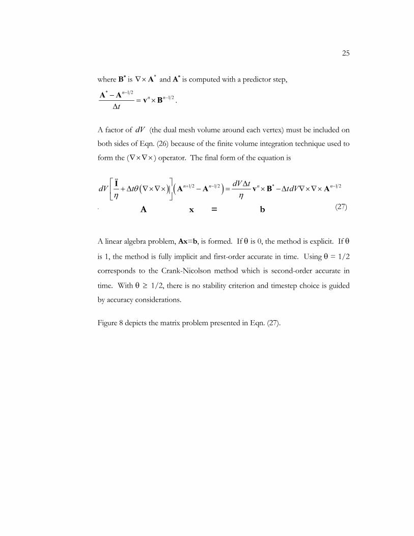
8. Basic matrix problem structure in MH4D .....................................................26
9. Operator matrix with conducting boundary conditions imposed .............31
10. Shear Alfvén wave simulation ..........................................................................34
11. Insulating boundary condition schematic ......................................................36
12. Operator matrix with insulating boundary condition ..................................39
13. Comparison of Spitzer and Chodura resistivity models ..............................41
14. MH4D kinetic energy growth rate predictions vs. resolution ....................47
15. MH4D screw pinch kinetic energy vs. time...................................................47
16. MH4D screw pinch simulation snapshot.......................................................48
17. Illustrations of tilt-stable and tilt-unstable spheromaks configurations....50
18. Spheromak m=1 tilt growth rates vs. L/R .....................................................50
19. Incorrect surface normal at corner of cylindrical spheromak domain......52
20. MH4D spheromak kinetic energy growth rates vs. resolution...................53
21. MH4D spheromak tilt simulation snapshot ..................................................53
22. Atomic physics simulation ionization fraction vs. time at 1.5 eV..............58
23. Spheromak kinetic energy vs. time with and without atomic physics.......59
24. Plasma mass vs. simulation time for spheromak with neutral gas.............60
iv
25. ZaP simulation diagram and MH4D 1/8-slice domain...............................62
26. Conceptual diagrams of ZaP Z-pinch formation .........................................63
27. Computational effort with implicit induction advance................................66
28. Current profiles for MH4D and MACH2 ZaP simulations .......................69
29. MACH2 ZaP simulation acceleration region behavior................................70
30. MACH2 ZaP simulation assembly region behavior.....................................71
31. “Coarse” MH4D ZaP simulation acceleration region behavior ................73
32. “Coarse” MH4D ZaP simulation assembly region behavior .....................74
33. “Fine” MH4D ZaP simulation acceleration region behavior.....................75
34. “Fine” MH4D ZaP simulation acceleration region behavior.....................76
35. 3D gas “puff” ZaP initial condition ................................................................79
36. Density evolution with 3D gas puff initial condition...................................81
37. Imacon images of plasma symmetrization in ZaP acceleration .................82
38. Snapshots of ZaP acceleration region simulation with neutral gas ...........83
39. Plasma mass and neutral mass vs. time for acceleration region
simulation with neutral gas................................................................................ 84
v
LIST OF TABLES
Table Number Page
1. Characteristic parameters for HIT-SI, ZaP and TCS ..................................13
2. MH4D screw pinch kinetic energy growth rates vs. linear stability
code predictions ..................................................................................................46
3. MH4D coronal equilibrium predictions compared to literature................57
4. Implicit advance accuracy with various timestep sizes ................................65
5. Comparison of ZaP simulation conditions for MACH2 and MH4D......68
vi
ACKNOWLEDGMENTS
Of the Aeronautics and Astronautics faculty, the author would like to give special
thanks to Professors Uri Shumlak, Tom Jarboe, Brian Nelson, and Research
Scientist George Marklin for the patience and expertise that they have offered in
support of this research. In addition, my thanks go to the PSI-Center Research
Consultants for their devotion, to my fellow Research Assistants and
Postdoctoral Research Associates, interaction with whom has been invaluable, to
Roberto Lionello, Dalton Schnack, the initial developers of MH4D, to the DOE
for supporting this work, and to my parents, family and friends who have always
had confidence in me to pursue and reach my dreams.
1
Introduction
The first significant plasma science research was conducted in the 1920’s by
Irving Langmuir. Since then, many plasma applications have been
commercialized – fluorescent lighting, plasma spray coating, and semi-conductor
manufacturing to name a few. However, magnetic fusion energy (MFE), a
plasma technology that would bring the power of stars to the earth, remains
elusive. The United States has committed a large part of its MFE research budget
to a single concept, the tokamak [1]. Because the commercial potential of the
tokamak is uncertain, Emerging Concept (EC) devices, intended to be simpler
and cheaper alternatives to the tokamak, are also being developed. The
computational modeling research described in this thesis has been performed as
part of the United States EC program.
Theorists have long relied on computation to improve comprehension of the
intertwined electromagnetic and gas dynamic interactions in plasmas. Because of
steadily increasing computer capability, it is now conceivable to simulate the
overall behavior of plasma in an MFE device. Significant progress toward this
goal has made, but integrated simulations that capture the small-scale and large-
scale phenomena that determine confinement quality are still under development.
The research for this thesis is part of the Plasma Science and Innovation (PSI)
Center collaboration, which develops predictive computational models of
emerging concept EC experiments [2].
The computational tool, MH4D (MagnetoHydrodynamics on a Tetrahedral
Domain), is the basis for the research described in this thesis. MH4D solves the
Resistive Magnetohydrodyamic (MHD) equations on a 3D tetrahedral mesh using
a finite volume scheme. MH4D’s irregular tetrahedral mesh facilitates grid
generation for complicated asymmetric 3D geometries. When acquired by the
2
PSI-Center, the code was capable of simulations with resistivity and viscosity in
domains with conducting boundaries. The following features have been added to
the code:
• Periodic and electrically insulating boundary conditions
• Variable resistivity in the form of Spitzer and Chodura models
• Ohmic heating
• A simple atomic physics model, including ionization and recombination of a
static neutral gas
Though the set of physics features in MH4D is smaller than for some similar
established codes (e.g. NIMROD), if a user would like to capture first order
Resistive MHD physics, the code’s relative simplicity is attractive. Periodic and
insulating boundary conditions can now be easily applied, and the capability of
the code has been explored and expanded. MH4D is a useful code, especially as
a test bed for new physics such as the atomic physics described in this thesis.
Several aspects of this research distinguish it from previous work:
1) This research involves full 3D MHD code development.
Full 3D codes (e.g. MACH3 [3] and WARP3 [4]) have previously been
developed. However, fusion plasma simulation research has focused primarily on
“spectral 3D” codes like NIMROD and M3D, which use 2D grids and resolve
the 3rd dimension spectrally. (As discussed later in this section, MH4D is further
distinguished from other full 3D code research by working with an irregular
tetrahedral mesh.) As compared to full 3D codes, spectral 3D codes are more
3
computationally efficient if low mode representation is adequate. Another
advantage of the spectral approach is that only 2D grid generation is required. A
limitation of spectral codes is that they require axisymmetry. Many MFE devices
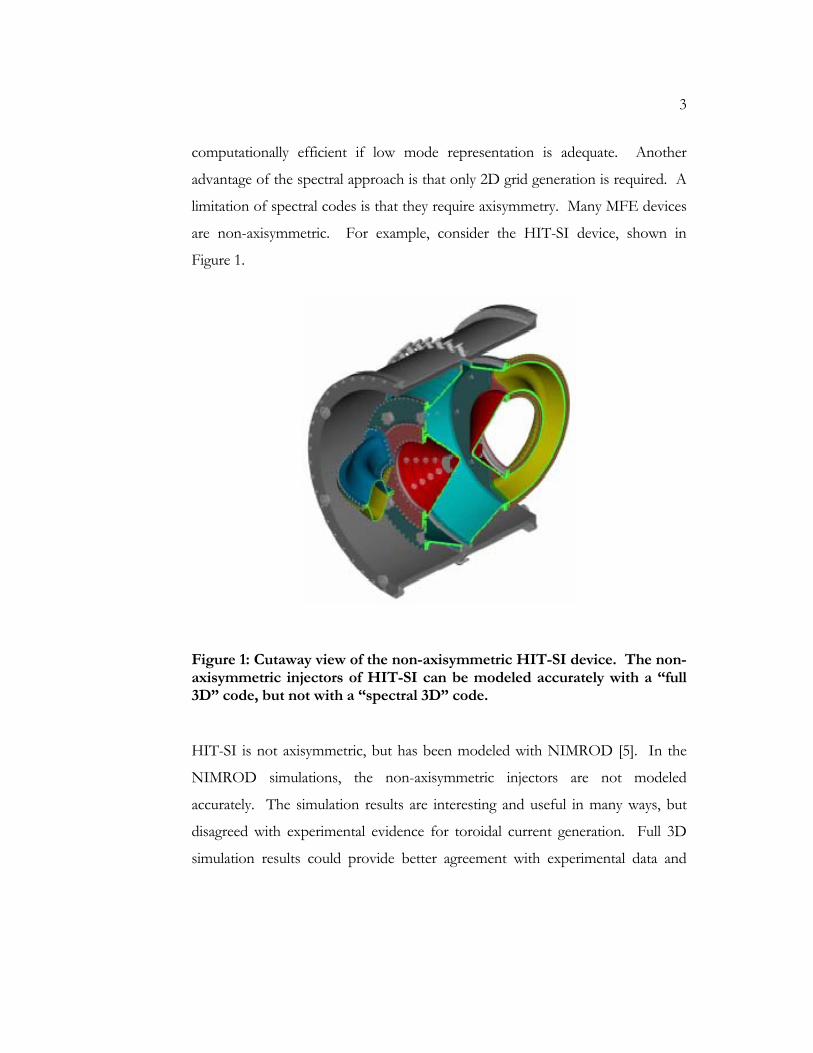
are non-axisymmetric. For example, consider the HIT-SI device, shown in
Figure 1.
Figure 1: Cutaway view of the non-axisymmetric HIT-SI device. The non-axisymmetric injectors of HIT-SI can be modeled accurately with a “full 3D” code, but not with a “spectral 3D” code.
HIT-SI is not axisymmetric, but has been modeled with NIMROD [5]. In the
NIMROD simulations, the non-axisymmetric injectors are not modeled
accurately. The simulation results are interesting and useful in many ways, but
disagreed with experimental evidence for toroidal current generation. Full 3D
simulation results could provide better agreement with experimental data and
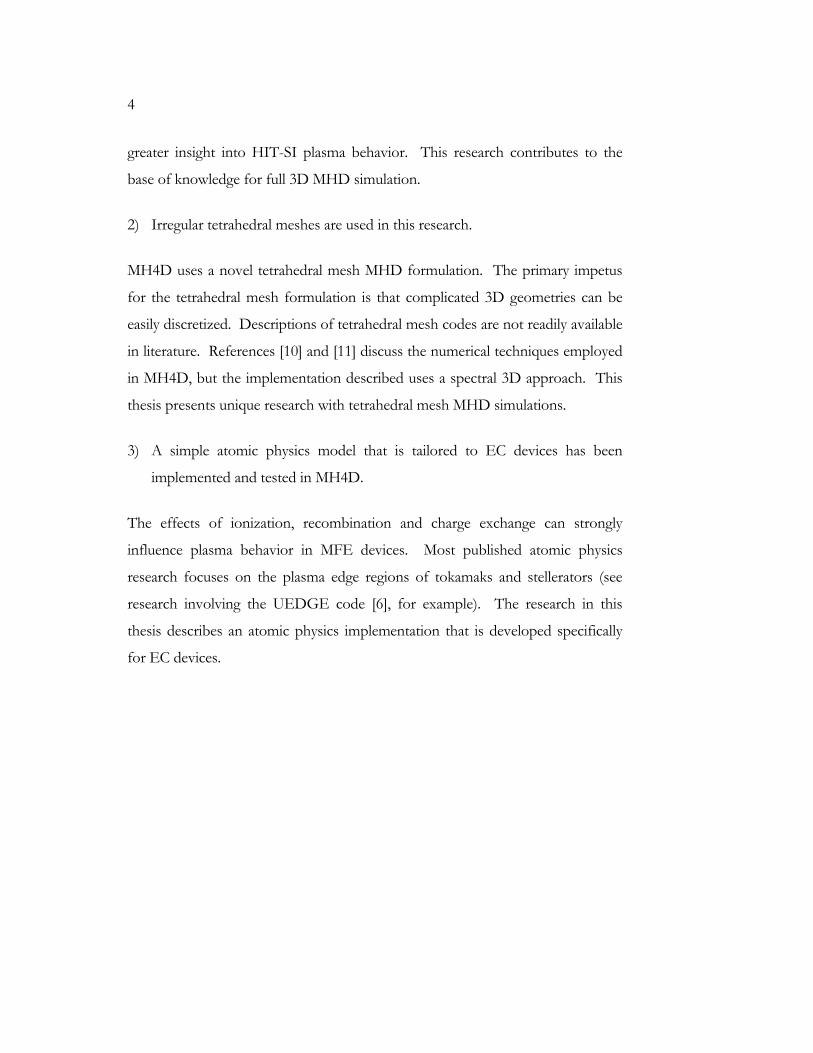
4
greater insight into HIT-SI plasma behavior. This research contributes to the
base of knowledge for full 3D MHD simulation.
2) Irregular tetrahedral meshes are used in this research.
MH4D uses a novel tetrahedral mesh MHD formulation. The primary impetus
for the tetrahedral mesh formulation is that complicated 3D geometries can be
easily discretized. Descriptions of tetrahedral mesh codes are not readily available
in literature. References [10] and [11] discuss the numerical techniques employed
in MH4D, but the implementation described uses a spectral 3D approach. This
thesis presents unique research with tetrahedral mesh MHD simulations.
3) A simple atomic physics model that is tailored to EC devices has been
implemented and tested in MH4D.
The effects of ionization, recombination and charge exchange can strongly
influence plasma behavior in MFE devices. Most published atomic physics
research focuses on the plasma edge regions of tokamaks and stellerators (see
research involving the UEDGE code [6], for example). The research in this
thesis describes an atomic physics implementation that is developed specifically
for EC devices.
5
Chapter 1
MAGNETOHYDRODYNAMICS (MHD) IN GENERAL
Section 1.1 introduces the reader to magnetohydrodynamics (MHD), briefly
describing its derivation from the particle picture. A more comprehensive
derivation can be found Krall and Trivelpiece [7]. Section 1.2 presents validity
limits for Resistive and Ideal MHD, largely following derivations by Freidberg [8].
Section 1.3 discusses these validity limits. In Section 1.4, the MHD validity limits
are applied to three EC experiments, HIT-SI, ZaP, and TCS.
1.1 From N-body models to MHD
N-body models, which track individual particle motion, and kinetic models,
which treat the plasma using probability distribution functions, are
computationally demanding and generally can not be used to simulate magnetic
fusion energy (MFE) devices. Fluid models are a common simplification of N-
body models. The quantities that are commonly thought of as “fluid properties”
– density, velocity, and temperature – are formally defined by taking moments of
the probability distribution function of a plasma. Moments of the Boltzmann
Equation, which is derived from a statistical plasma picture, produce the
equations of the fluid models. The first three moments yield the density,
momentum, and energy equations. Higher moments are possible, but these three
are commonly used for a reasonably complete model that is computationally
tractable. The equation set is closed with an equation of state – e.g. the adiabatic
equation of state, p γρ∝ . If the density, momentum and energy equations are
tracked for ions and electrons, the equation set is called the Two-Fluid Model.
6
To reach the Full (Single-Fluid) Magnetohydrodynamic Model, or Full MHD,
two “asymptotic approximations” are made:
1) Assume that the permittivity of free space is approximately zero. This
enforces “quasineutrality” and eliminates displacement current in Ampere’s Law.
2) Assume that electron mass is approximately zero.
Implications of these approximations are discussed in Section 1.2. The first
asymptotic approximation results in the low-frequency Maxwell’s equations,
0 , , 0t
µ ∂∇× = ∇× = − ∇ • =
∂BB J E B . (1)
In addition to these Maxwell’s equations, Full MHD has a density equation,
vρρ•−∇=
∂∂t
, (2)
a momentum equation,
( )i ept
ρ ∂ + •∇ + ∇ − × = −∇ • + ∂ v v v J B π π (3)
an Ohm’s law (derivation of which involves neglecting electron momentum per
the second asymptotic approximation),
( )1e ep
Zenη+ × = + × − ∇ − ∇ •E v B J J B π (4)
and a pressure equation,
( )1 : :
ei ie i e i i e e
e
e
d p Q Qdt
pZen
γ γ
γ
γρ ρ
ρ
− = + − ∇ • + − ∇ − ∇
+ •∇
h h π v π v
J, (5)
7
where eπ and iπ are anisotropic pressure tensors for the electrons and ions, η is
electrical resistivity, Z is effective ion charge, e is electron charge, n is electron
number density, eh and ih are heat fluxes for electrons and ions, and eiQ and
ieQ represent electron-ion and ion-electron collisional heating. To reach the
Ideal MHD model, all terms on right-hand sides of Eqns. (3), (4), and (5) are
neglected. Of the terms neglected to reach the Ideal MHD, the Resistive MHD
model retains the term involving electrical resistivity (η j) in Eqn. (4) and an
Ohmic heating term ( 2~ η j ) associated with eiQ . Along with the modified
Maxwell’s equations as given in Eqn. (1), the Resistive MHD model uses Eqns.
(2)-(5) in reduced form,
E η= − ×J v B
( ) ( ) 21 ( 1)p p pt
γ γ η∂+ ∇ • = − ∇ • + −
∂v v j
vρρ•−∇=
∂∂t
pt
ρ ∂ + •∇ = −∇ + × ∂ v v v J B . (6)
Resistive MHD provides the basis for MH4D. The particular form of the model
used in MH4D is presented in Section 2.1.
1.2 Validity Limits of Ideal and Resistive MHD
Several assumptions were made in deriving Ideal MHD. Implications of these
assumptions are discussed below, and key validity limits are presented. The basis
for the limits is shown in some of the most important cases. Details supporting
each validity limit can be found in reference [8].
Ohm’s Law
Pressure
Continuity
Momentum
8
To develop validity limits, it is necessary to define and specify several
characteristic quantities for the plasma of interest. Characteristic time and length
scales, τ and L, are set. Characteristic magnetic field, density, temperature, speed,
and resistivity (B0, ρ0, T0, and V0) are also defined. Although these scales and
parameters are subjective choices1, validity limits still provide valuable insight into
MHD limitations.
Maxwellian distributions
In the process of deriving Ideal and Resistive MHD, Maxwellian distributions are
assumed for ions and electrons. For these assumptions to be valid, electron and
ion collisionality must be high: 1 and 1ii eeτ ττ τ
, where iiτ is the ion-ion
collision time, eeτ is the electron-electron collision time, and τ is the
characteristic timescale of phenomena of interest. The ion collisionality
requirement,
1iiττ
, (7)
is more restrictive than the electron collisionality requirement.
First asymptotic approximation
Under the first approximation, Maxwell’s equations are transformed to the low-
frequency Maxwell’s equations2. This is implemented by allowing the permittivity
of free space to equal zero. Gauss’s Law and Ampère’s Law are modified. In
1 For instance, the characteristic magnetic field, B0,, chosen for a Z-pinch might be the maximum field value.
However, B=0 at the center of a Z-pinch, so the choice for B0 is clearly not valid throughout the plasma. Similar general estimates are made for density, resistivity, and temperature for all experiments evaluated.
2 As discussed, this approximation packages two simplifications: the assumption of quasineutrality and elimination of displacement current. These two simplifications can be considered independently as in reference [7].
9
Gauss’s Law, which can be written 0 q nα αα
ε ∇ • = ∑E , 0 0ε ≈ means that
0q nα αα
≈∑ . This implements local quasineutrality, but does not require that
0∇ • =E or that E be restricted in any way. Next, consider Ampère’s Law with
the electric field split into dynamic and steady components,
( )00
1s d
t tε
µ∂ ∂ + = ∇× − ∂ ∂
E E B j . 0 0ε ≈ does not pertain to Es because
0s
t∂
=∂E without the assumption. The dynamic electric field in Ampère’s Law is
eliminated, implying that electrons respond quickly to prevent local charge
separation. Note that electric fields can still exist and evolve (slowly) under this
first approximation.
The first approximation implies that 2
0 0
1cµ ε
= → ∞ and 2
2
0pe
e
nem
ωε
= → ∞ .
Therefore, only phenomena with characteristic speeds 0V c and characteristic
times 1
pe
τω
are captured under this assumption. It should be noted that
high-frequency phenomena can affect low-frequency phenomena occurring on
the timescale of interest. (High-frequency effects can sometimes be captured
with transport coefficients such as resistivity as described in Section 3.4.)
Second asymptotic approximation
Under the second approximation, electron mass is set to zero. This
approximation is natural since the ratio of proton mass to electron mass is 1836.
However, electron mass causes finite response times which are significant,
especially over long distances. Low-frequency, long-wavelength modes caused by
10
electron lag, called drift waves, are missed in the MHD model because of this
second approximation.
If 0em → , clearly 2
2
0pe
e
nem
ωε
= → ∞ and cee
eBm
ω = → ∞ . It follows that
electron skin depth, 0epe
clω
= → , electron Larmor radius, , 0th eLe
ce
vr
ω= → , and
Debye length, , 0th eD
pe
vλ
ω= → . Therefore, only phenomena with
1 1,pe ce
τω ω
and characteristic length ( ), ,e Le DL l r λ are captured under
this assumption. As mentioned above in the discussion of the first
approximation, high-frequency phenomena can affect low-frequency phenomena.
Hall and diamagnetic terms
In Ohm’s Law, Zen×J B (the Hall term) and ep Zen∇ (the diamagnetic term)
are neglected. Validity can be assessed by comparing these terms to a retained
term in Ohm’s Law, ×v B . These assumptions are valid if
2
2~ 1x
ce elZenL
τω×J Bv B
, (8)
~ 1xe Lip Zen r
L∇
v B. (9)
Infinite conductivity
In Ohm’s Law, it is assumed that η=0. This assumption is valid if
0 0 .
1~ 1x RemagLVη η
µ=
jv B
. (10)
11
Collisional heating
The collision heating terms, eiQ and ieQ , include the effects of Ohmic heating
and from thermodynamic equilibration of the electron and ion species. If Eqn.
(10) is violated, Ohmic heating should be included. Ions and electrons are in
thermodynamic equilibrium if
1iii em m τ
τ. (11)
This thermodynamic equilibrium limit is more restrictive by i em m than the
collisionality limit given by Eqn. (7).
Heat fluxes
e∇ •h dominates the total heat flux ( )e i∇ • +h h . The validity of neglecting
e∇ •h is assessed by comparing e∇ •h to p t∂ ∂ . For validity, 1iii em m τ
τ.
This limit is identical to the thermodynamic equilibrium limit, Eqn. (11).
Electron convection
The term e
e
pZen γρ
•∇
J can be neglected if 1LirL
. This is the same validity
limit found for the diamagnetic term.
Anisotropic terms in energy equation
:i i∇π v can be neglected if the ion collisionality limit, Eqn. (7), is satisfied. The
requirement for neglecting :e e∇π v is less restrictive.
12
1.3 Discussion of MHD validity limits
The high collisionality requirement is usually not met for fusion grade plasmas.
However, empirical evidence indicates that Ideal/Resistive MHD are useful
beyond the high collisionality validity limit. This circumstance arises because
cyclotron motion plays the role of collisions in most fusion plasmas, and
enhances the effective collisionality perpendicular to magnetic fields. In general,
if parallel gradients are not expected, the collisionality assumption can be relaxed.
An important shortcoming of Ideal/Resistive MHD is an inability to capture
local charge separation and the associated “two-fluid” effects such as the Lower
Hybrid Drift instability.
To summarize, Ideal/Resistive MHD captures low-frequency, large-scale
phenomena, and its simplicity makes it a valuable tool for understanding
macroscopic plasma behavior.
13
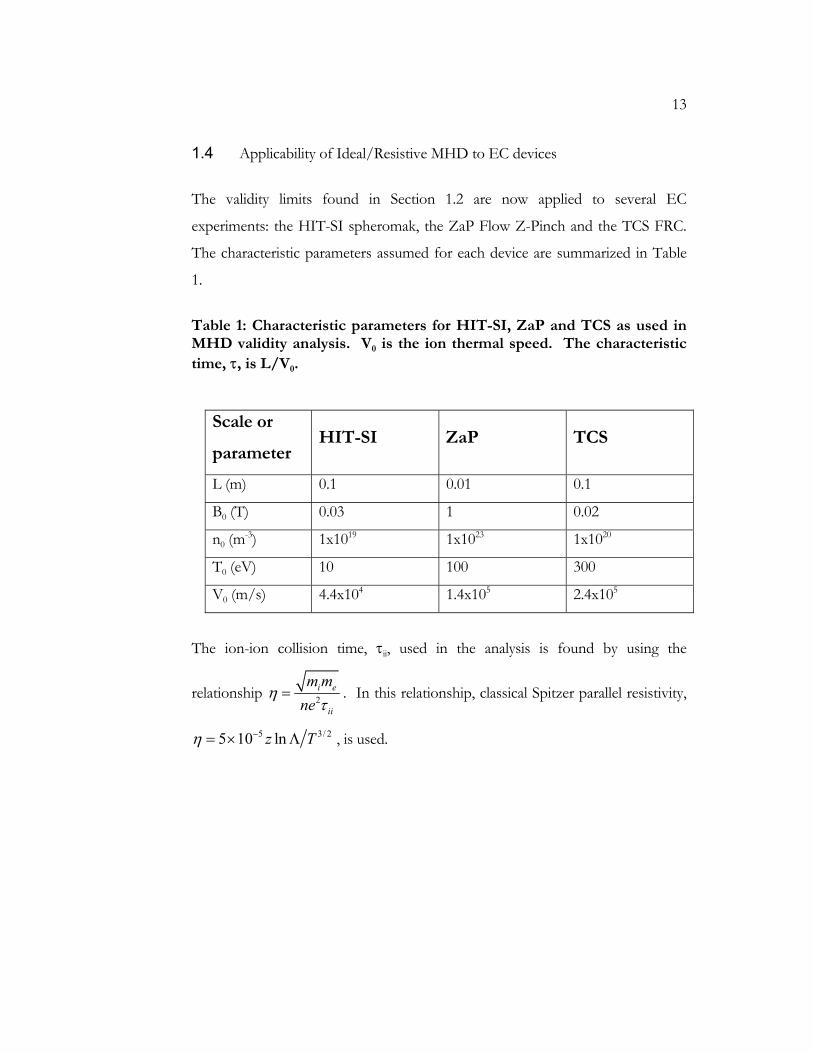
1.4 Applicability of Ideal/Resistive MHD to EC devices
The validity limits found in Section 1.2 are now applied to several EC
experiments: the HIT-SI spheromak, the ZaP Flow Z-Pinch and the TCS FRC.
The characteristic parameters assumed for each device are summarized in Table
1.
Table 1: Characteristic parameters for HIT-SI, ZaP and TCS as used in MHD validity analysis. V0 is the ion thermal speed. The characteristic time, τ, is L/V0.
Scale or
parameter HIT-SI ZaP TCS
L (m) 0.1 0.01 0.1
B0 (T) 0.03 1 0.02
n0 (m-3) 1x10¹⁹ 1x10²³ 1x10²⁰
T0 (eV) 10 100 300
V0 (m/s) 4.4x10⁴ 1.4x10⁵ 2.4x10⁵
The ion-ion collision time, τii, used in the analysis is found by using the
relationship 2i e
ii
m mne
ητ
= . In this relationship, classical Spitzer parallel resistivity,
5 3/ 25 10 lnz Tη −= × Λ , is used.
14
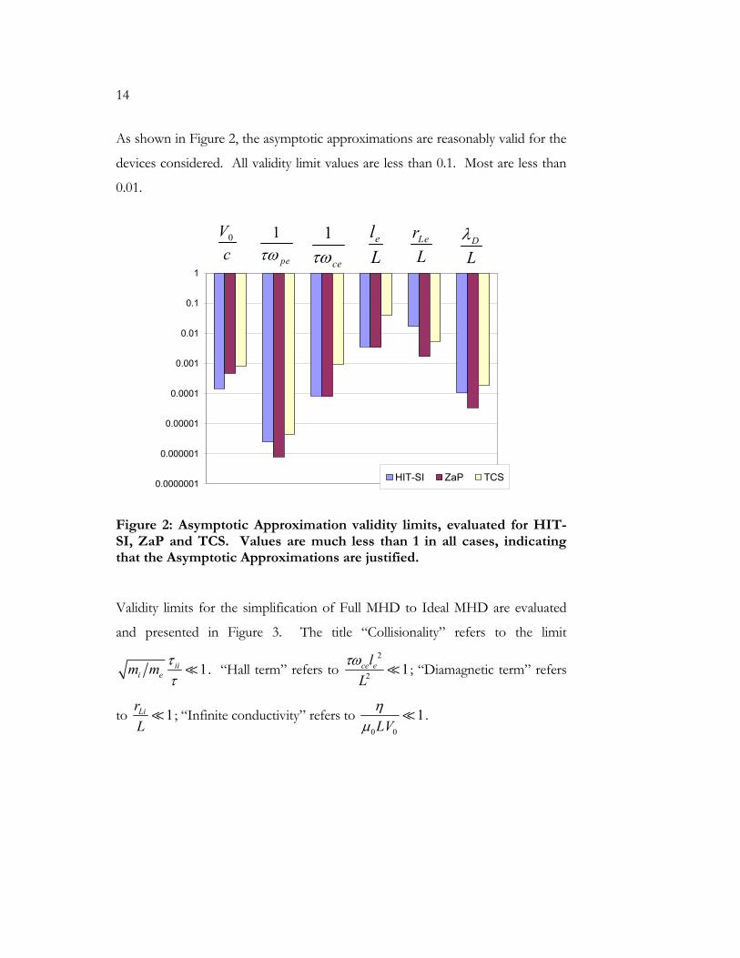
As shown in Figure 2, the asymptotic approximations are reasonably valid for the
devices considered. All validity limit values are less than 0.1. Most are less than
0.01.
0.0000001
0.000001
0.00001
0.0001
0.001
0.01
0.1
1
HIT-SI ZaP TCS
Figure 2: Asymptotic Approximation validity limits, evaluated for HIT-SI, ZaP and TCS. Values are much less than 1 in all cases, indicating that the Asymptotic Approximations are justified.
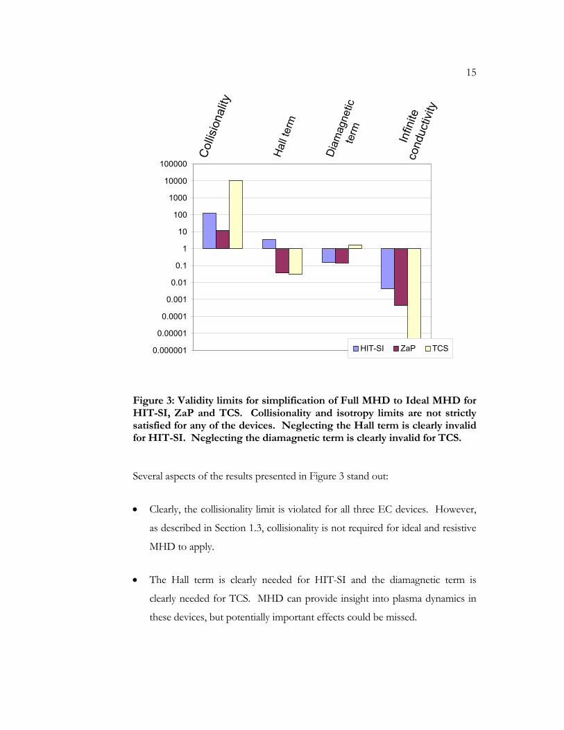
Validity limits for the simplification of Full MHD to Ideal MHD are evaluated
and presented in Figure 3. The title “Collisionality” refers to the limit
1iii em m τ
τ. “Hall term” refers to
2
2 1ce elL
τω ; “Diamagnetic term” refers
to 1LirL
; “Infinite conductivity” refers to 0 0
1LVη
µ.
0Vc
1
peτω1
ceτωelL
LerL
D
Lλ
15
0.000001
0.00001
0.0001
0.001
0.01
0.1
1
10
100
1000
10000
100000
HIT-SI ZaP TCS
Figure 3: Validity limits for simplification of Full MHD to Ideal MHD for HIT-SI, ZaP and TCS. Collisionality and isotropy limits are not strictly satisfied for any of the devices. Neglecting the Hall term is clearly invalid for HIT-SI. Neglecting the diamagnetic term is clearly invalid for TCS.
Several aspects of the results presented in Figure 3 stand out:
• Clearly, the collisionality limit is violated for all three EC devices. However,
as described in Section 1.3, collisionality is not required for ideal and resistive
MHD to apply.
• The Hall term is clearly needed for HIT-SI and the diamagnetic term is
clearly needed for TCS. MHD can provide insight into plasma dynamics in
these devices, but potentially important effects could be missed.
Col
lisio
nalit
y
Hal
l ter
m
Dia
mag
netic
term Infin
iteco
nduc
tivity

16
• Figure 3 indicates that resistivity can be neglected in the three EC devices.
Core plasma characteristics are assumed in Figure 3. However, plasma
characteristics are dramatically different at the plasma edge and in near-
vacuum regions, and the infinite conductivity validity limit is not applicable.
For instance, in ZaP, high resistivity is appropriate in vacuum regions and in
cool plasma.
17
Chapter 2
MH4D OVERVIEW
MH4D is a plasma simulation code that solves the resistive MHD equations with
a finite volume method [23] on a tetrahedral mesh. The code is parallelized.
T3D [24] is used to generate the mesh. ParMETIS [18] is used for partitioning.
PETSc [26] is used for parallel matrix computations. Key algorithms include
leapfrog time discretization, predictor-corrector advance to provide dissipation in
the induction equation, and implicit treatment of dissipative terms. In this
chapter, the features of MH4D that existed before adoption by the PSI-Center
are presented, and some practical code application issues are discussed. Features
that have been developed by the PSI-Center are described in Chapter 3.
2.1 MHD in original MH4D
MH4D originally used the following Resistive MHD model:
t∂
− =∂A E , AB ×∇= , = ∇×j B (12)
tη∂
= × −∂A v B j
p p pt
γ∂+ •∇ = − ∇ •
∂v v
vρρ•−∇=
∂∂t
2pt
ρ ν∂ + •∇ = −∇ + × + ∇ ∂ v v v j B v ,
where A is the magnetic vector potential, B is the magnetic field, E is the electric
field, v is velocity, j is current density, p is pressure, is ρ density, η is electrical
Induction
Pressure
Continuity
Momentum
18
resistivity, and ν is viscosity. A is the primitive variable for the electromagnetic
components of the code. MH4D normalizes j and B by 0µ so that µ0 is left
out of the computations. This results in conversions from “MH4D” units to S.I.
units as shown in Appendix A.1.
MH4D uses a Cartesian coordinate system.
2.2 Tetrahedral mesh and finite volume formulation
MH4D uses an irregular tetrahedral mesh, a particularly useful mesh type when
the computational domain involves complex geometric features. To generate a
useful 3D mesh often requires separately discretizing different regions of the
domain and then ensuring appropriate interfaces between the regions. With
tetrahedra, the domain can be discretized as a single region and special interfacing
is not required. Ease of grid generation comes at a price:
• Computational overhead is increased.
o Reference arrays (see Appendix A.2) are required to describe the
irregular grid. Logically mapped grids require no such arrays.
• Solution accuracy at a given resolution can be compromised.
o Although first-order accuracy is maintained in a tetrahedral mesh
with distorted tetrahedra, a uniform mesh may produce smoother
solutions in general.
Eqns. (12) are solved in the order shown. Integral relations are used to define the
operators. For example, the gradient is
∫∫ =∇SV
dSfdVf )()( n (13)
19
In original MH4D algorithm development (i.e. before the research for this thesis
began), special care was taken to preserve analytical properties of MHD in the
discretized equations. In particular, the discretized spatial operators are self-
adjoint [10]. Self-adjoint operators allow application of the efficient conjugate
gradient method in iterative implicit solves.
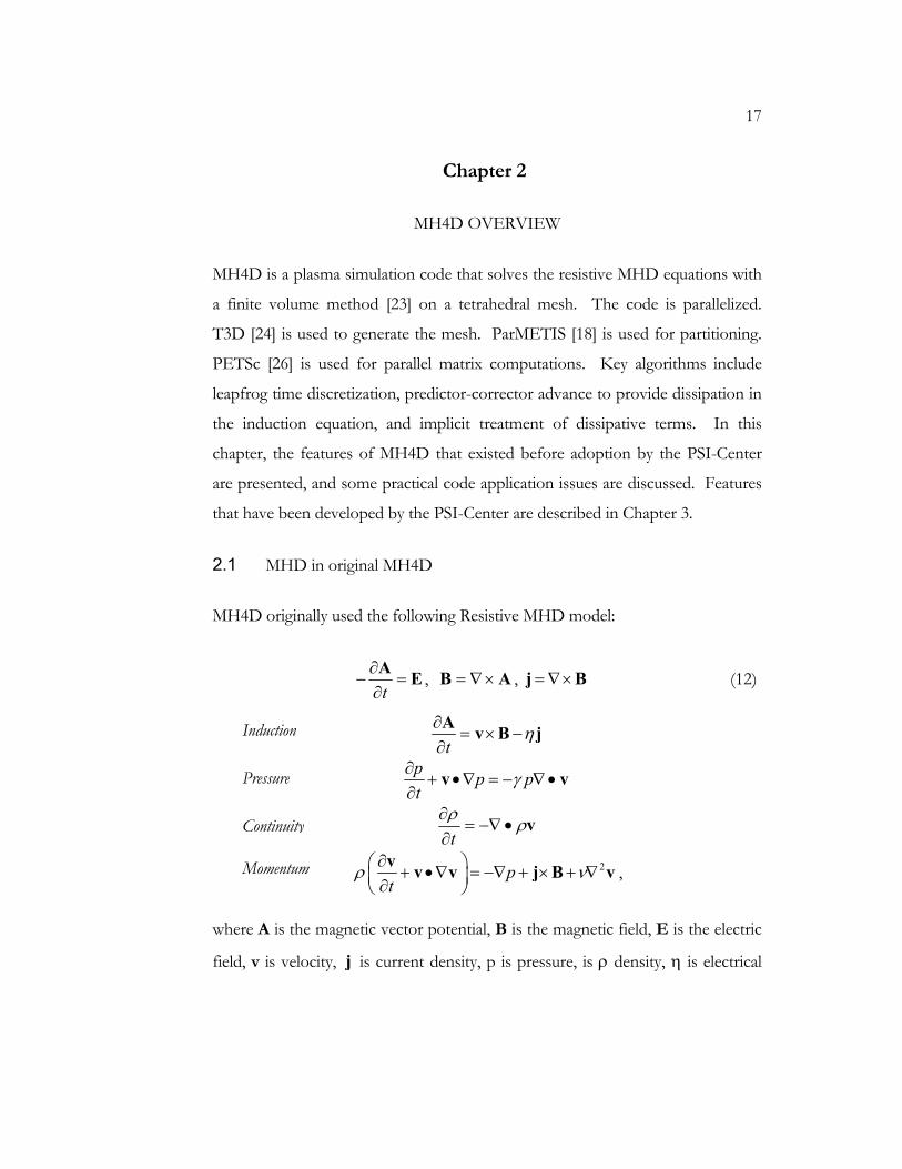
Figure 4 shows a tetrahedron as used by MH4D. A staggered mesh or “dual
mesh” is defined by the dashed lines between edge midpoints, side centroids and
the cell centroid. Sides are labeled by the index of their opposite vertex. C is the
centroid of the tetrahedron. mij is the midpoint of edge lij. Ci is the centroid of
side i. Si is the vector area of side i. si is the vector area of the dual mesh surface.
Appendix A.3 provides additional geometric details which are used in the MH4D
finite volume formulation.
Figure 4: Staggered mesh used in MH4D. Vertices, edge lengths, tetrahedron surface areas, a dual mesh surface area, edge midpoints, face centroids, and the tetrahedron centroid are labeled.
20
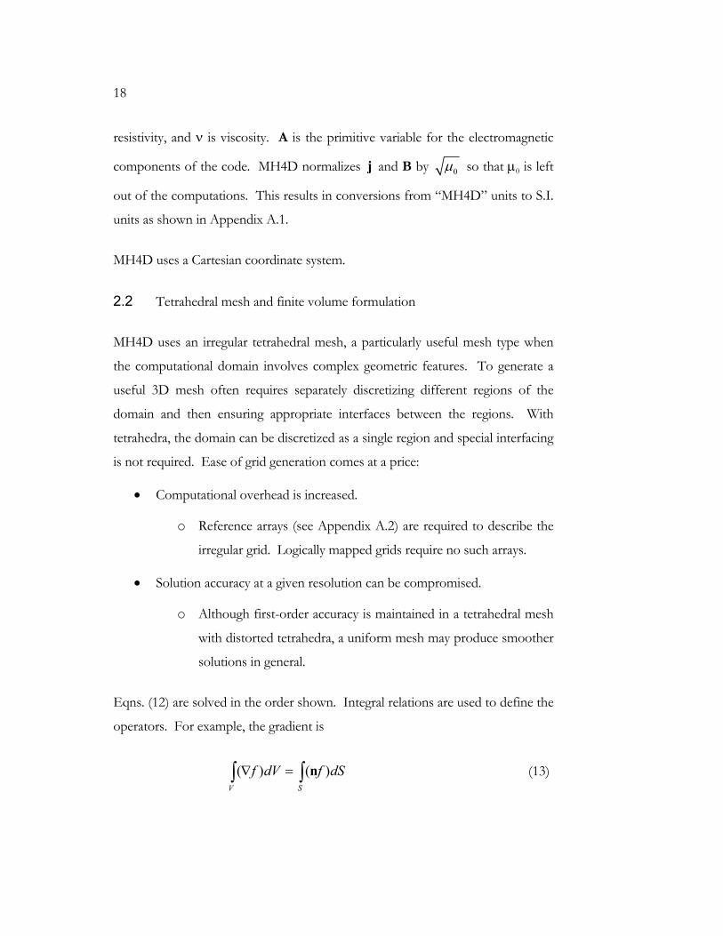
As shown Figure 5, density, pressure and magnetic field are stored at cell
centroids. Vector potential, momentum and current density are stored at vertices.
Averaging is used to determine velocity at edge midpoints and at face centers as
required for advection as described below.
Figure 5: Variable storage locations. All variables are stored at either centroids or vertices. Velocity is averaged to centroids and faces for advection calculations.
Applying the finite volume method with B stored at tetrahedron centroids and A
stored at vertices results in 0∇ • =B inside the domain. (No such guarantee
exists for ∇ • B on boundaries.) See Appendix A.3 for details.
21
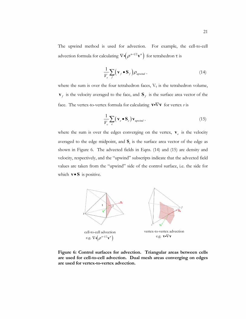
The upwind method is used for advection. For example, the cell-to-cell
advection formula for calculating ( )1 2n nρ −∇ vi for tetrahedron τ is
( )1f f upwind
fVτ
ρ•∑ v S , (14)
where the sum is over the four tetrahedron faces, Vτ is the tetrahedron volume,
fv is the velocity averaged to the face, and fS is the surface area vector of the
face. The vertex-to-vertex formula for calculating ∇v vi for vertex v is
( )1e e upwind
evV•∑ v S v , (15)
where the sum is over the edges converging on the vertex, ev is the velocity
averaged to the edge midpoint, and Se is the surface area vector of the edge as
shown in Figure 6. The advected fields in Eqns. (14) and (15) are density and
velocity, respectively, and the “upwind” subscripts indicate that the advected field
values are taken from the “upwind” side of the control surface, i.e. the side for
which •v S is positive.
Figure 6: Control surfaces for advection. Triangular areas between cells are used for cell-to-cell advection. Dual mesh areas converging on edges are used for vertex-to-vertex advection.
vertex-to-vertex advection e.g. ∇v vi
cell-to-cell advectione.g. ( )1 2n nρ −∇ vi
22
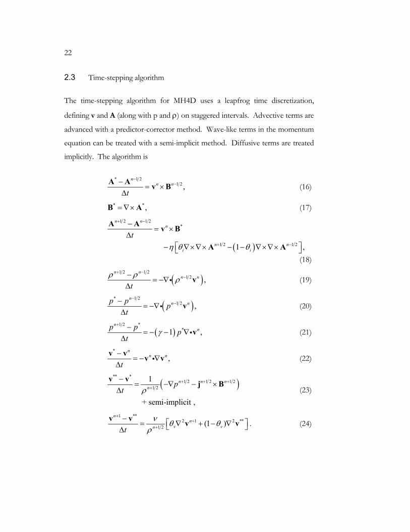
2.3 Time-stepping algorithm
The time-stepping algorithm for MH4D uses a leapfrog time discretization,
defining v and A (along with p and ρ) on staggered intervals. Advective terms are
advanced with a predictor-corrector method. Wave-like terms in the momentum
equation can be treated with a semi-implicit method. Diffusive terms are treated
implicitly. The algorithm is
* 1 21 2 ,
nn n
t
−−−
= ×∆
A A v B (16)
* *,= ∇×B A (17)
( )
1 2 1 2*
1 2 1 2 1 ,
n nn
n ni i
tη θ θ
+ −
+ −
−= ×
∆ − ∇×∇× − − ∇×∇×
A A v B
A A (18)
( )1 2 1 2
1 2 ,n n
n n
tρ ρ ρ
+ −−−
= −∇∆
vi (19)
( )* 1 2
1 2 ,n
n np p pt
−−−
= −∇∆
vi (20)
( )1 2 *
*1 ,n
np p pt
γ+ −
= − − ∇∆
vi (21)
*
,n
n n
t−
= − ∇∆
v v v vi (22)
( )** *
1 2 1 2 1 21 2
1
+ semi-implicit ,
n n nn p
t ρ+ + +
+
−= −∇ − ×
∆v v j B
(23)
1 **2 1 2 **
1 2 (1 )n
nv vnt
ν θ θρ
++
+
− = ∇ + − ∇ ∆v v v v . (24)
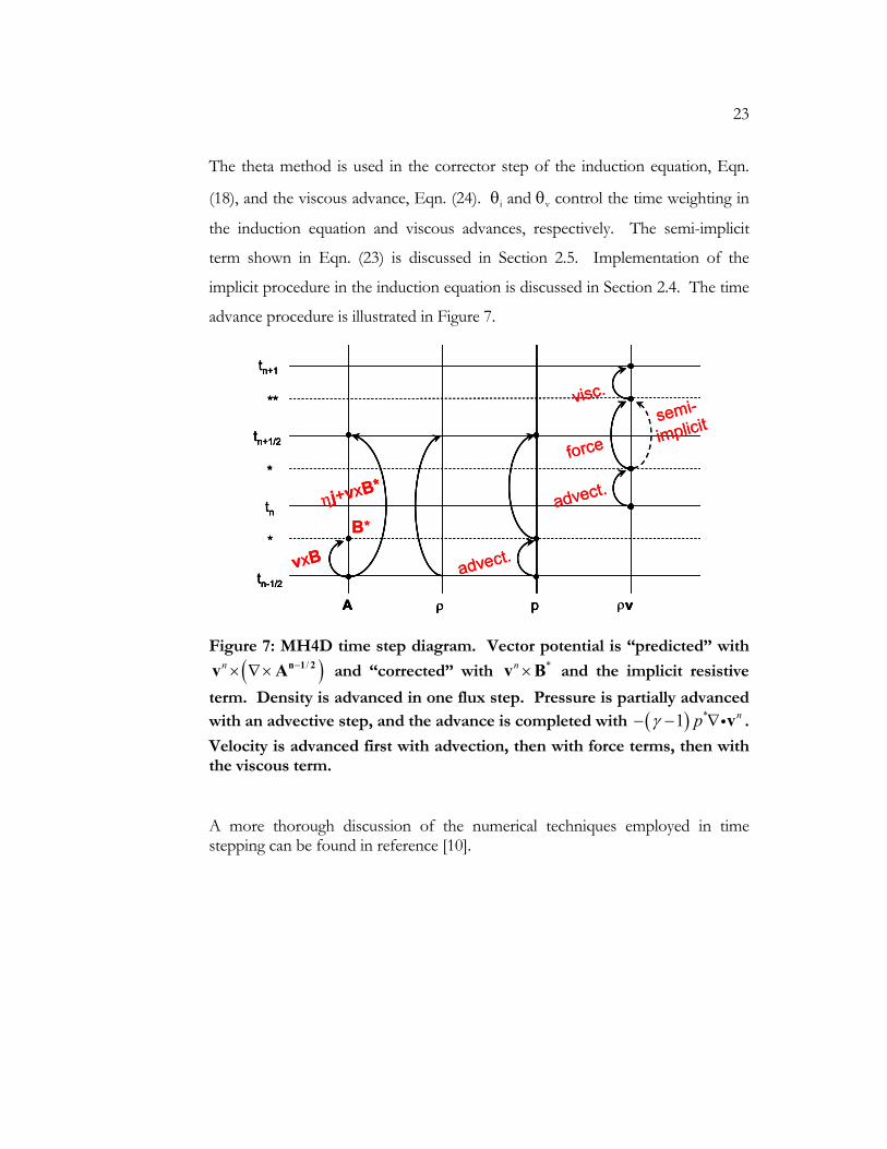
23
The theta method is used in the corrector step of the induction equation, Eqn.
(18), and the viscous advance, Eqn. (24). θi and θv control the time weighting in
the induction equation and viscous advances, respectively. The semi-implicit
term shown in Eqn. (23) is discussed in Section 2.5. Implementation of the
implicit procedure in the induction equation is discussed in Section 2.4. The time
advance procedure is illustrated in Figure 7.
tn-1/2
tn
tn+1/2
tn+1
*
*
**
A ρ p v
tn-1/2
tn
tn+1/2
tn+1
*
*
**
A ρ p v
vxB
B*ηj+vxB*
advect.
force
visc.
advect.
semi-
implicit
ρ
tn-1/2
tn
tn+1/2
tn+1
*
*
**
A ρ p v
tn-1/2
tn
tn+1/2
tn+1
*
*
**
A ρ p v
vxB
B*ηj+vxB*
advect.
force
visc.
advect.
semi-
implicit
ρ
Figure 7: MH4D time step diagram. Vector potential is “predicted” with
( )/n −× ∇× n 1 2v A and “corrected” with *n ×v B and the implicit resistive
term. Density is advanced in one flux step. Pressure is partially advanced with an advective step, and the advance is completed with ( ) *1 npγ− − ∇ vi .
Velocity is advanced first with advection, then with force terms, then with the viscous term.
A more thorough discussion of the numerical techniques employed in time stepping can be found in reference [10].
24
2.4 Implicit resistive diffusion advance
An implicit advance of the resistive diffusion term of induction equation is
appropriate when, because of numerical stiffness, excessive computational effort
is required to advance the equation explicitly. Numerical stiffness in the
induction equation is introduced by high resistivity. The ( )η ∇×∇× A term in
the induction equation is diffusive as seen if a vector identity is used to rewrite
the term as
( ) ( ) 2η η η∇×∇× = ∇ ∇ • − ∇A A A . The 2∇ operator is the 3D equivalent of
the spatial second derivative in the 1D diffusion equation, 2
2
u uDt x
∂ ∂=
∂ ∂, where u
is a generic variable quantity and D is a diffusion coefficient. As shown in [25],
the timestep limit
2
2xtD
∆∆ ≤ (25)
must be observed if the 1D diffusion equation is solved explicitly. In three
dimensions, the ∆x is replaced with the grid spacing, i.e. the distance between the
vertices on which A is stored. For fine meshes, this diffusive timestep limit is
often much more prohibitive than other timestep limits such as the Courant
limits discussed in Section 2.5.
MH4D uses a θ-method for advancing A. In time-discretized form, the equation
is
( )1 2 1 2
* 1 2 1 21n n
n n n
tη θ θ
+ −+ −− = × − ∇×∇× + − ∇×∇× ∆
A A v B A A , (26)
25
where B* is *∇× A and A* is computed with a predictor step, * 1 2
1 2n
n n
t
−−−
= ×∆
A A v B .
A factor of dV (the dual mesh volume around each vertex) must be included on
both sides of Eqn. (26) because of the finite volume integration technique used to
form the (∇×∇× ) operator. The final form of the equation is
( ) ( )1 2 1 2 * 1 2n n n ndV tdV t tdVθη η
+ − − ∆+ ∆ ∇×∇× − = × −∆ ∇×∇×
I A A v B A
. (27)
A linear algebra problem, Ax=b, is formed. If θ is 0, the method is explicit. If θ
is 1, the method is fully implicit and first-order accurate in time. Using θ = 1/2
corresponds to the Crank-Nicolson method which is second-order accurate in
time. With θ ≥ 1/2, there is no stability criterion and timestep choice is guided
by accuracy considerations.
Figure 8 depicts the matrix problem presented in Eqn. (27).
A x b=
26
=
C1111 C1112 C1113
C1121 C1122 C1123
C1131 C1132 C1133
C12 C1n
Cnn
C21
Cn1
x1,1x1,2x1,3
xn,1xn,2xn,3
b1,1b1,2b1,3
bn,1bn,2bn,3
=
C1111 C1112 C1113
C1121 C1122 C1123
C1131 C1132 C1133
C12 C1n
Cnn
C21
Cn1
x1,1x1,2x1,3
xn,1xn,2xn,3
b1,1b1,2b1,3
bn,1bn,2bn,3
Figure 8: Basic matrix problem structure in MH4D. The matrix, A, is an n x n matrix of 3 x 3 coupling matrices, Cij, coupling each vertex i to itself and all other vertices j. The components of vector quantities in x and b are labeled 1, 2 and 3.
For interior points, the vector components 1, 2 and 3 shown in Figure 8 are just
the x, y, and z Cartesian components. For boundary points, vector quantities are
stored in a rotated frame such that the z axis is normal to the boundary surface –
in this rotated frame, vector components 1 and 2 are tangential to the boundary
surface and component 3 is normal to the surface. This facilitates boundary
condition application as discussed in Section 2.6.
The matrix A is symmetric positive definite: Cii=CiiT and Cij=Cji
T. Thus,
convergence of the Conjugate Gradient method is guaranteed. MH4D uses
PETSc to invert symmetric positive definite matrices using a preconditioned
Conjugate Gradient method.
A x = b
27
To understand the matrix shown in Figure 8, it is important to know the nature
of the self-adjoint ( )dV ∇×∇× operator. It is shown below operating on A to
give dVj at vertex i:
( ) ( )1 19i i i i v i i v v
v
dV dVV
τ τ τ τ τ
τ τ
= ∇×∇× = − − • • ∑ ∑j A S S S S I A (28)
where subscripts v and τ represent vertices and tetrahedra, S represents surface
area vectors, and V is volume. The inner sum is over the vertices, v, of a
tetrahedron, τ, and the outer sum is over the tetrahedra that share vertex i. The
3x3 coupling matrices Cij shown in Figure 8 account for each contribution in
Eqn. (28). Geometric details supporting Eqn. (28) and other MH4D finite
volume relations are available in Appendix A.3.
2.5 Semi-implicit momentum advance
This section is an introduction to the semi-implicit advance used in MH4D.
Details are provided in references [27], [28], and [29]. Validation of the semi-
implicit method in MH4D for sound wave and Alfvén wave test problems is
described in [30].
If the resistive term of the induction equation is treated implicitly and momentum
is advanced explicitly, the algorithm shown in Section 2.3 is numerically stable if
the simulation timestep satisfies the Courant conditions for waves and flows,
maxv t x∆ < ∆ (29)
28
where maxv depends on the flow speed, flowv , and on the magnetosonic wave
speed, 2 2MS A Sv v v= + , where the subscripts A and S refer to the Alfvén and
sound speeds. maxv is defined by the geometric mean, 2 2max MS flowv v v= + . The
magnetosonic wave speed is often much faster than the flow speed. However,
using a semi-implicit method, the magnetosonic wave speed dependence in Eqn.
(29) can be eliminated, leaving max flowv v= .
The full MHD operator can separated into fast and slow components:
u u u ut
∂= = +
∂M F S . (30)
Alfvén waves and sound waves are contained in F , the fast part of the operator,
while S contains the slower physics of interest. By treating F implicitly, the
prohibitive wave Courant condition can be avoided. This procedure – treating
fast waves implicitly and slow/interesting dynamics explicitly – is called semi-
implicit3. Discretizing in time, treating the fast part implicitly (i.e. letting it
operate on the velocity at time n+1), and treating the slow part explicitly,
( )
11 1
1
n nn n n n
n n n
u u u u u ut
u u u
++ +
+
−= + = +
∆= + −
F S F M -F
M F, (31)
This equation can be rewritten as a matrix problem for 1n nu u+ − ,
3 The semi-implicit method was developed for weather modeling, as described in [31], to eliminate the
timestep restriction due to fast gravity waves.
full MHD operator Alfvén waves, soundwaves
interesting physics
29
( )( ) 1n n nt u u t u+− ∆ − = ∆I F M . (32)
nuM is explicitly calculated, and the equation is solved implicitly for 1n nu u+ −
by inverting ( )t− ∆I F . F is chosen such that the matrix ( )t− ∆I F is self-
adjoint and can be solved with PETSc using a preconditioned Conjugate
Gradient algorithm. Using the semi-implicit method, the computational effort
can be significantly less than the effort required for an explicit advance.
The semi-implicit algorithm in MH4D was not used in this research. As
mentioned above, the algorithm was used successfully in wave simulations, but
additional research will be required to develop the algorithm for general
applications like the benchmark simulations described in this research.
2.6 Boundary conditions
MH4D sets boundary conditions in two ways. Explicit boundary conditions are
applied after explicit calculations, e.g. by zeroing normal components at
boundaries. Implicit boundary couplings are modified in coupling matrices used in
implicit advances that involve boundary points.
Nodes and sides are flagged in MH4D to facilitate boundary condition
implementation. The code as originally adopted by the PSI-Center had only
(perfectly) electrically conducting boundaries. All boundary nodes and sides are
flagged. At all boundaries, vector quantities are stored in a rotated coordinate
system with the z component normal to the surface4.
4 Domain corners present a challenge because the surface normal is undefined. Special treatment is often
required at corners.
30
At perfectly conducting boundaries, tangential E must be zero. Thus, tangential
components of t
∂∂A are set to zero5.
The boundary condition for pressure is that the normal gradient is zero. Parallel
velocity can be allowed on all boundaries (a slip boundary condition), or set to
zero on all boundaries (a no-slip boundary condition). Normal velocity is set to
zero on all conducting boundaries. Pressure and density flux are not allowed at
any boundary.
Perfectly conducting wall boundary conditions are imposed in MH4D by default.
For instance, before vxB is used to advance A, the subroutine zero_bndr_vv is
called to zero the tangential components of vxB on boundaries. Also,
zero_normal_vv is used to zero normal velocity at conducting boundaries. Non-
default explicit boundary conditions are set using routines in setbc.f. For
instance, special boundary conditions required at domain corners are imposed in
setbc.f.
Conducting boundary conditions require tangential 0=E . Therefore, implicit
boundary conditions are applied to the matrix ( )dV tθη
+ ∆ ∇×∇×
I in Eqn.
(27). Figure 9 illustrates the modifications made to impose conducting boundary
conditions. Tangential components of conducting boundary vertices are
decoupled from the equation system. Notice that the modified matrix remains
symmetric positive definite.
5 The condition Etangential=0 corresponds to a fixed Atangential as shown in Eqn. 12.
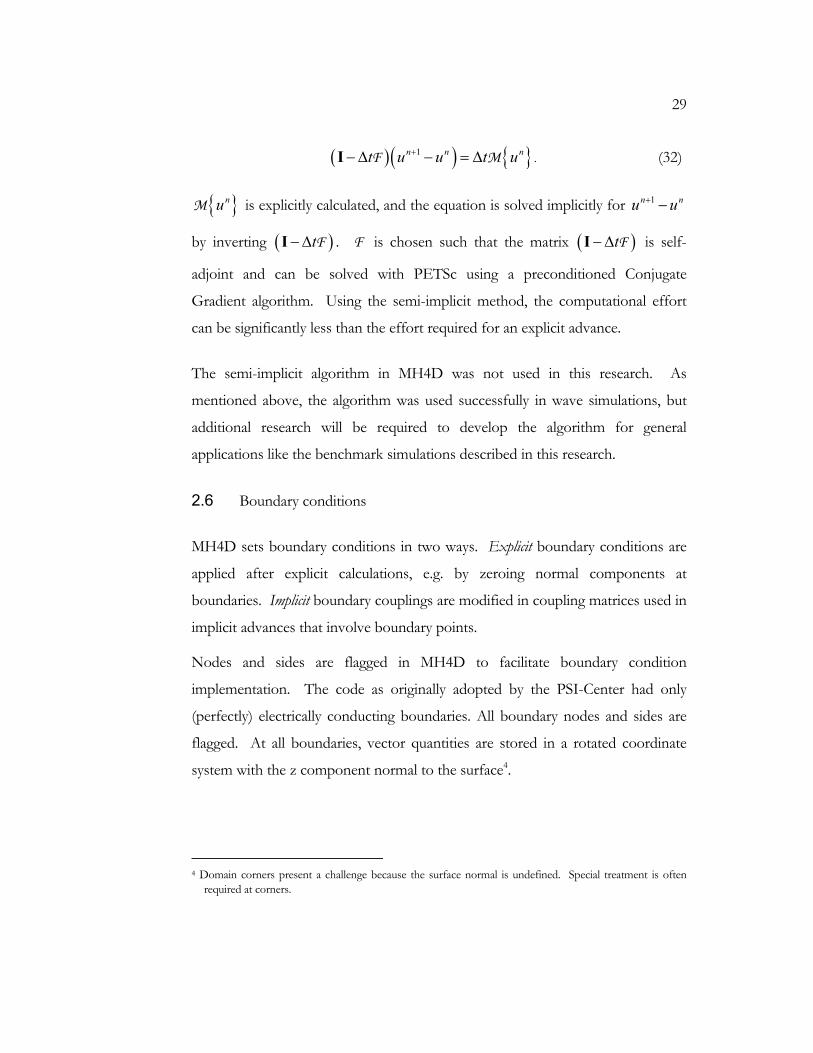
31
=
1 0 00 1 00 0 n
C1n
CnnCn1
x1,1x1,2x1,3
xn,1xn,2xn,3
00
b1,3
bn,1bn,2bn,3
C22
0 0 n0 0 n0 0 n
0 0 00 0 0n n n
=
1 0 00 1 00 0 n
C1n
CnnCn1
x1,1x1,2x1,3
xn,1xn,2xn,3
00
b1,3
bn,1bn,2bn,3
C22
0 0 n0 0 n0 0 n
0 0 00 0 0n n n
Figure 9: Operator matrix with conducting boundary condition imposed. Vertex 1 is on a conducting boundary. Vertex 2 is an interior vertex. Tangential components of conducting boundary vertices are decoupled.
2.7 Practical issues in MH4D simulations
Input deck
Through the input deck, all key variables can be set without recompiling the code.
Timestep
Typically, a small timestep (~10x less than the timestep required to satisfy stability
limits) is used initially. The setdt routine allows the code to increase the timestep
incrementally (the fractional increase never exceeding 10%) to the user-defined
fraction of the timestep stability limit set with the input deck values, cflfac,
cflfac_imp, or cflfac_si. The more restrictive of the wave/flow timestep limits
and the resistive timestep limit is imposed by the setdt routine.
32
Grids and restart files
The grid generation program T3D [24] is used to create T3D files as described in
Appendix B. A T3D file contains information about vertex/tetrahedron
association and location. The “load” reads the T3D file and produces a “restart”
file with grid information and MH4D primitive variable information in General
Mesh Viewer (GMV) format [21] or in Tecplot [22] format. Data postprocessing
involves reading restart files with GMV or Tecplot.
Different input parameters can be used with the load program to initialize a
variety of problems. Reflect, shift, and rotate routines are available to manipulate
the grid.
Memory considerations
MH4D is parallelized, and the memory requirements during the time stepping
loop depend directly on the degree of parallelization. However, in the setup
process, each processor temporarily creates and stores reference arrays and
geometric factors describing the entire grid. Presently, setup is performed in
parallel. For grids with many million tetrahedra, it may be important to modify
MH4D so that setup processing occurs in serial so that memory limits are not
exceeded.
33
Chapter 3
CODE DEVELOPMENT
3.1 Periodic boundary condition
Periodic boundary conditions are an important feature for a plasma simulation
code. For example, computational expense can be reduced, mode selection is
possible, and wave simulation is facilitated. The periodic boundary condition
implemented in MH4D allows multi-direction periodicity which is needed for
Alfvén wave simulation. The implementation also allows non-parallel-plane
periodicity. Azimuthal sections of axisymmetric domains can be modeled,
enabling mode selection and domain size reduction. For example if a 1/4-slice of
a cylindrical domain is simulated, only m=0, 4, 8, etc. modes are captured.
In MH4D, periodicity has been implemented for pairs of periodic surfaces. One
of the surfaces is designated “redundant” and the other, “retained”. On the
retained surfaces, grid entities (vertices, triangular tetrahedral sides, and
tetrahedral edges) are kept. On the redundant surfaces, redundant entity
information is eliminated and replaced by pointers to the appropriate retained
entities.
Two test problems were used to verify functionality of the parallel-plane periodic
boundary condition: a sound wave and a shear Alfvén wave. For example, the
Alfvén wave perturbation is
1 2cos( ) sin( )t tkε
ω ε ω∧ ∧
= • − ⊥ ⇒ = • − ⊥1 1A k x B k x
2sin( )tε ω∧
= • − ⊥1v k x (33)
34
where 2
∧
⊥ and 1
∧
⊥ are in the transverse direction, ε is the perturbation size, k is
a wavevector in the longitudinal direction. ( 2 nLπ
=k where n is the mode
number and L is the periodic length.)
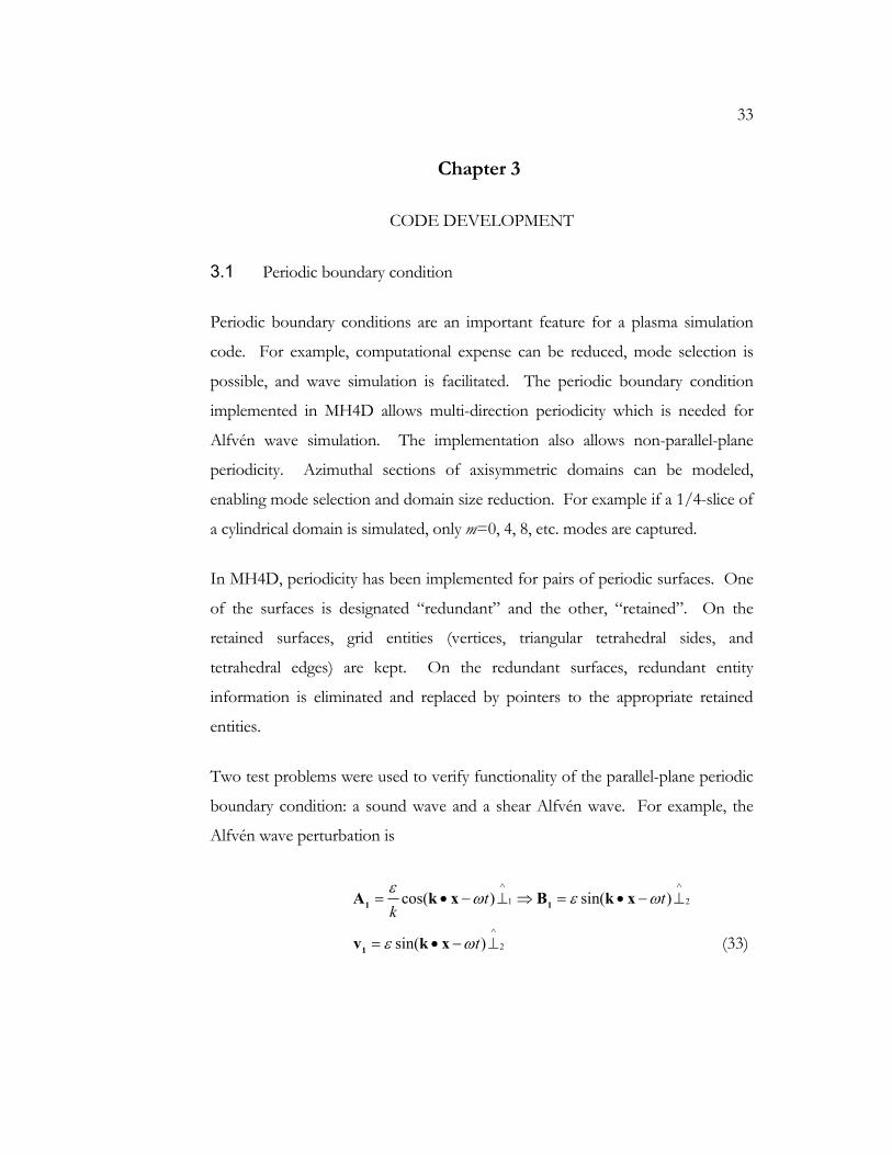
An obliquely propagating shear Alfvén wave in a triply periodic box domain was
simulated successfully as depicted in Figure 10.
Figure 10: Perpendicular magnetic field strength contours for a shear Alfvén wave.
Non-parallel-plane periodicity is implemented by rotating vector quantities across
the periodic boundary as appropriate, and by zeroing perpendicular components
of vector quantities on the periodic axis. Rotations are simple in explicit
calculations – the rotated (or inverse-rotated) quantity is multiplied by a rotation
matrix. Rotations for matrix couplings across boundaries are more complicated.
Consider the calculation
ij j i=C x b , (34)
35
where Cij is a 3x3 matrix which multiplies vector xj to give vector bi. If the vector
at vertex j is in a rotated frame defined by the rotation matrix Rj, and the vector at
vertex i is in a rotated frame defined by the rotation matrix Ri, the calculation is
( ) ( )T Tij j j i i=C R x R b , (35)
where RT is the transposed rotation matrix. This can be rewritten
( )T Ti ij j j i=R C R x b . (36)
The coupling matrix is pre-multiplied by TiR and post-multiplied by T
jR , and
now vectors xj and bi are in their rotated frames. Additional care must be taken if
the vectors x or b are on boundary points (recall that the boundary vectors are
rotated such that their third vector component is normal to the surface). In this
case, the inverse boundary rotation must take place before rotation across the
periodic boundary.
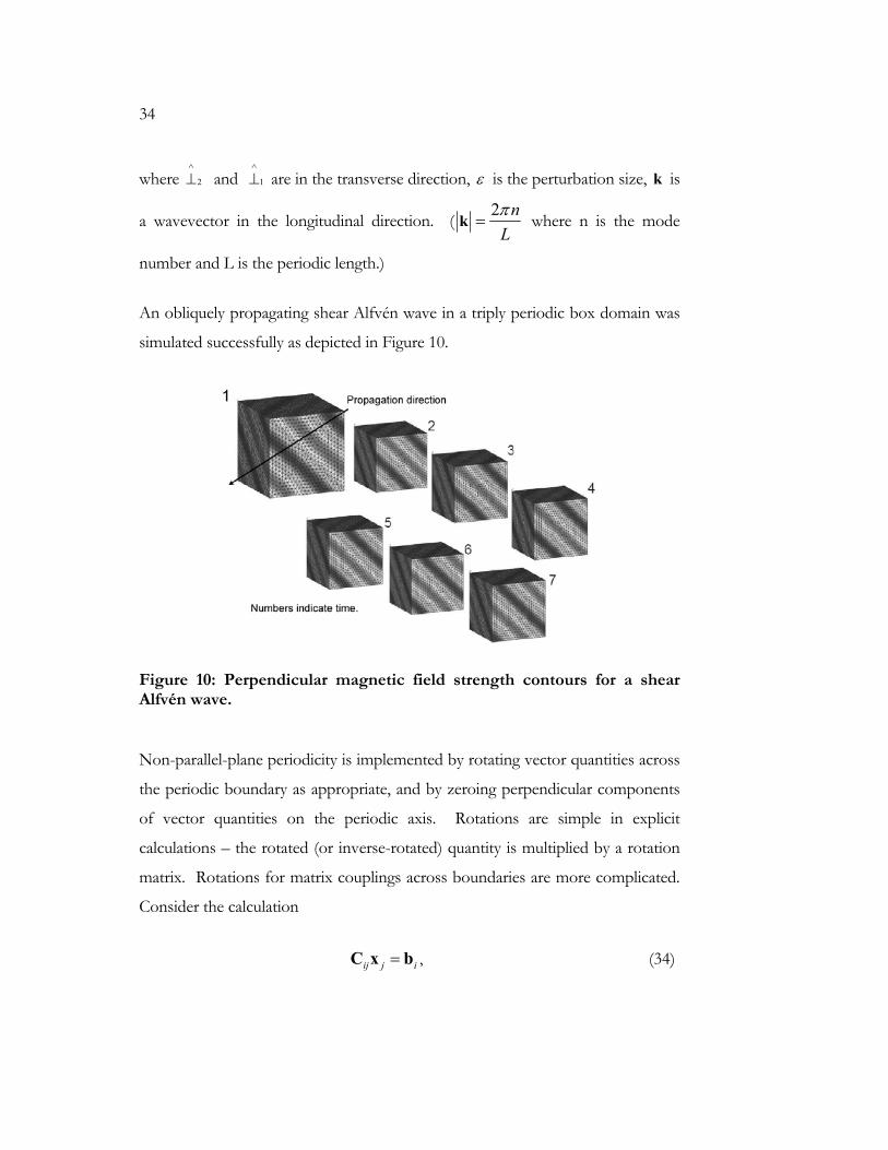
3.2 Insulating boundary condition
An insulating-wall boundary condition has been added such that plasma
interaction with electrically isolated electrodes can be modeled. To initially
develop the boundary condition, a plasma-armature railgun was modeled as
shown in Figure 11. The method was then extended to coaxial cylindrical shell
electrodes and to ZaP simulations (see Chapter 6).
36
Bx (applied)
jy (induced)
Bx (applied)
jy (induced)
Figure 11: Plasma armature railgun problem with insulating boundary. Applied magnetic field, Bx, corresponds to a current source as shown. Top and bottom boundaries are electrically conducting. Gray-shaded boundaries are electrically insulating. The jxB force drags the applied Bx into the domain ( “flux injection”).
In general, either an electric or a magnetic field can be specified on the insulating
boundary. If an electric field is specified, a fixed voltage across the electrodes is
implied. If the magnetic field is specified, constant current is dictated between
the electrodes. For instance, in coaxial geometry, 02 enclosedrB Iθπ µ= . In many
plasma experiments, the power-supply has much higher impedance than the
plasma, and the total current applied is a smoother function than the applied
voltage. For this reason, the specified magnetic field boundary condition has
been developed in MH4D.
Inside the domain, the current density at vertex i is calculated with the following
formula:
13i i
vVτ
τ
= ×∑J S B , (37)
37
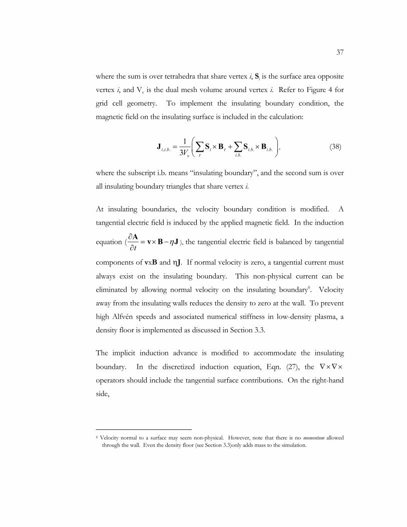
where the sum is over tetrahedra that share vertex i, Si is the surface area opposite
vertex i, and Vv is the dual mesh volume around vertex i. Refer to Figure 4 for
grid cell geometry. To implement the insulating boundary condition, the
magnetic field on the insulating surface is included in the calculation:
, . . . . . .. .
13i i b i i b i b
i bvVτ
τ
= × + × ∑ ∑J S B S B , (38)
where the subscript i.b. means “insulating boundary”, and the second sum is over
all insulating boundary triangles that share vertex i.
At insulating boundaries, the velocity boundary condition is modified. A
tangential electric field is induced by the applied magnetic field. In the induction
equation (t
η∂= × −
∂A v B J ), the tangential electric field is balanced by tangential
components of vxB and ηJ. If normal velocity is zero, a tangential current must
always exist on the insulating boundary. This non-physical current can be
eliminated by allowing normal velocity on the insulating boundary6. Velocity
away from the insulating walls reduces the density to zero at the wall. To prevent
high Alfvén speeds and associated numerical stiffness in low-density plasma, a
density floor is implemented as discussed in Section 3.3.
The implicit induction advance is modified to accommodate the insulating
boundary. In the discretized induction equation, Eqn. (27), the ∇×∇×
operators should include the tangential surface contributions. On the right-hand
side,
6 Velocity normal to a surface may seem non-physical. However, note that there is no momentum allowed
through the wall. Even the density floor (see Section 3.3)only adds mass to the simulation.
38
( ) ( )internal boundary∇×∇× = ∇×∇× + ∇×∇×A A A , (39)
where the insulating boundary term, ( )boundary∇×∇× A is . . . .
. .
13 i b i b
i bvV×∑B S as
found in Eqn. (38). On the left-hand side of Eqn. (27), (∇×∇× ) acts on
( )1 2 1 2n n+ −−A A , so the surface part is ( )1 2 1 2. . . . . .
. .
13
n ni b i b i b
i bvV+ −− ×∑ B B S . Assuming
that Bi.b. is slowly varying on the boundary, Eqn. (27) is unchanged except for
explicitly including the surface contribution for 1 2n−∇×∇× A per Eqn. (38). The
implicit boundary conditions imposed on the (∇×∇× ) operator must be
modified to allow for tangential components on the boundary. Recall that, as
shown in Figure 9, tangential boundary components are decoupled for
conducting boundary vertices. For insulating boundary vertices, tangential
components remain coupled and normal components are decoupled as shown in
Figure 12.
39
=
t t 0t t 00 0 1
C1n
CnnCn1
x1,1x1,2x1,3
xn,1xn,2xn,3
bn,1bn,2bn,3
C22
t t 0t t 0t t 0
t t tt t t0 0 0
b1,1b1,20
=
t t 0t t 00 0 1
C1n
CnnCn1
x1,1x1,2x1,3
xn,1xn,2xn,3
bn,1bn,2bn,3
C22
t t 0t t 0t t 0
t t tt t t0 0 0
b1,1b1,20
Figure 12: Operator matrix with insulating boundary condition imposed. Vertex 1 is on an insulating boundary. Vertex 2 is an interior vertex. Normal components of insulating boundary vertices are decoupled.
By decoupling normal components on the insulating boundary, a zero normal
electric field boundary condition is imposed. This implies that surface charge is
not allowed. Neglecting surface charge seems to be acceptable in the sense that
flux is injected and the calculation is numerically stable. However, allowing
surface charge (i.e. allowing normal components on the insulating boundary to
couple) was not studied and could also give reasonable results.
If 1 2. .ni b
+B is known, the assumption of slow variation of . .i bB is unnecessary. The
contribution of the surface term, ( )1 2 1 2. . . . . .
. .
13
n ni b i b i b
i bvV+ −− ×∑ B B S , is then added to
the right-hand side.
40
3.3 Density floor
As density approaches zero, Alfvén speed ( 0Av µ ρ= B ) approaches infinity.
After density is advanced, if density in any cell has dropped below some “density
floor”, mass is added at that cell to maintain the floor density. If the total mass
contribution is small, this violation of continuity is acceptable.
3.4 Resistivity models and ohmic heating
Only uniform resistivity was available when the PSI-Center began developing
MH4D. Options for Spitzer resistivity, Chodura resistivity, and a combination of
the two have been added. Spitzer resistivity is defined by the well-known formula
( )5
. 32
5 10 ln-mSp
eVTη
−× Λ= Ω (40)
The empirical Chodura resistivity model is designed to capture the anomalous
resistivity that occurs at low densities. This anomalous resistivity is attributable to
an instability when the electron drift speed exceeds the ion sound speed by a
factor of ~3. This was shown by Shumlak et al. in simulations using a Two-Fluid
plasma physics model [19] [20]. Chodura resistivity is implemented as
2neme
CC νη = ; , 1 exp ep iC C
s
vCfv
ν ω
= − −
(41)
where the electron drift speed and sound speed are e neν =
j and
ργν p
s = . The
Chodura constant, Cc, and the parameter f, are typically Cc ≈ 0.1 and f ≈ 3.
41
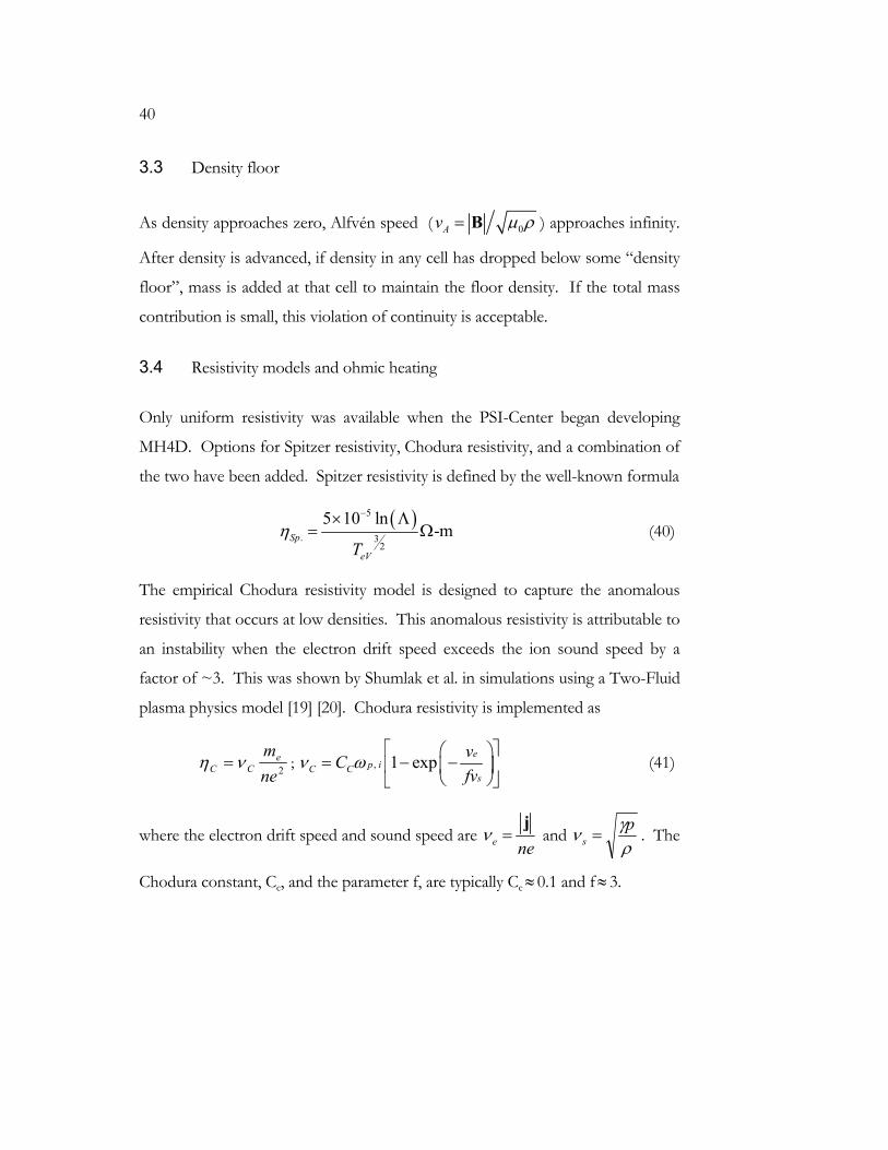
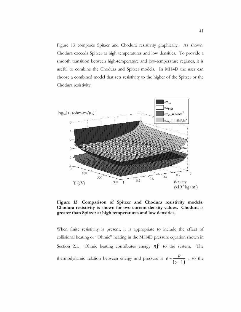
Figure 13 compares Spitzer and Chodura resistivity graphically. As shown,
Chodura exceeds Spitzer at high temperatures and low densities. To provide a
smooth transition between high-temperature and low-temperature regimes, it is
useful to combine the Chodura and Spitzer models. In MH4D the user can
choose a combined model that sets resistivity to the higher of the Spitzer or the
Chodura resistivity.
Figure 13: Comparison of Spitzer and Chodura resistivity models. Chodura resistivity is shown for two current density values. Chodura is greater than Spitzer at high temperatures and low densities.
When finite resistivity is present, it is appropriate to include the effect of
collisional heating or “Ohmic” heating in the MH4D pressure equation shown in
Section 2.1. Ohmic heating contributes energy 2η j to the system. The
thermodynamic relation between energy and pressure is ( )
~ peγ −1
, so the
T (eV) density (x10-3 kg/m3)
log10[ η (ohm-m/µ0) ]
42
contribution of Ohmic heating to pressure is ( ) 21γ η− j . The modified pressure
equation is
( ) 21p p pt
γ γ η∂+ •∇ = − ∇ • + −
∂v v j . (42)
3.5 Atomic physics
Neutral gas atoms can have a significant effect on plasma behavior in magnetic
confinement devices. Ionization cools the plasma. Ionized neutrals add mass
with low momentum, slowing plasma motion. Recombination and charge
exchange likewise play significant roles in plasma energy and momentum loss. By
adding atomic physics effects in order of importance, the PSI-Center intends to
develop an atomic physics model that allows predictive computational modeling
of EC devices. An initial step has been to implement in MH4D a simple model
involving a plasma fluid and a neutral fluid. The neutral fluid is assumed to be
stationary and cold. The induction equation is unchanged for this atomic physics
model. The new and modified equations are
( )ii i ion rect
ρ ρ∂= −∇ +Γ − Γ
∂vi (43)
nion rect
ρ∂= −Γ + Γ
∂ (44)
( )ii e i rec i ip p mt
ρ ∂+ ∇ + = × −Γ
∂v j B v (45)
( ) ( )21 1 ion n ion rec ip p p m m pt
γ γ η γ∂+ ∇ = − ∇ + − − − Γ Φ − Γ
∂v v ji i . (46)
43
Eqns. (43)-(46) are ion continuity, neutral continuity, ion momentum, and ion
pressure. Modifications to the usual MH4D MHD model are shown in boxes.
ionΓ and recΓ are the source rates for ionization and recombination in
( )3/kg m s . For example, i ion e i nnσ ρΓ = ⟨ ⟩v , where ionσ is the ionization cross
section and ion eσ⟨ ⟩v is the ionization rate parameter. The angle brackets indicate
that the quantity has been averaged over a Maxwellian distribution. Charge
exchange is assumed to be zero in this implementation, but could easily be added.
Ionization and recombination rates are temperature dependent per the following
relations for coronal equilibrium given by Goldston and Rutherford [9]:
1/ 213, 3 -1
, ,
2 10 13.6exp m s6.0 /13.6 13.6
e eVion e
e eV e eV
TT T
σ− ×
⟨ ⟩ = − + v (47)
1/ 2
19 3 -1
,
13.60.7 10 m srec ee eVT
σ − ⟨ ⟩ = ×
v (48)
Simple ion and neutral accounting rules are observed in MH4D. If iondtΓ is
greater than nρ , i i nρ ρ ρ= + and 0nρ = . Likewise, if recdtΓ is greater than iρ ,
n n iρ ρ ρ= + and n floorρ ρ= .
Timestep restrictions associated with atomic physics timescales are discussed in
Section 5.1.
A limitation of this atomic physics model is that Paschen physics (i.e. the cascade
of secondary electrons emitted by collisions in an interelectrode gap) is not
captured. However, as shown in the applications of this model (see Chapter 5
and Section 6.6), important atomic physics effects are still captured.
44
Chapter 4
SCREW PINCH AND SPHEROMAK BENCHMARKS
4.1 Screw Pinch
As a code benchmark test, the linear phase of the m=1 screw pinch kink
instability was simulated with MH4D. The instability growth rates found with
MH4D are compared to growth rates found with a linear stability analyzer which
uses the linearized MHD equations and captures only m=1 modes.
4.1.1 Theoretical Background
Equilibrium in a screw pinch is governed by the equation
p× = ∇j B (49)
There are three variables: p, the plasma pressure, Bθ, the azimuthal magnetic field,
and Bz, the axial magnetic field. (Radial magnetic field is zero.) If any two of
these are specified, the third is determined by the equilibrium equation.
Beginning with an equilibrium, we expect an external current-driven kink
instability in a screw pinch if the axial magnetic field is too weak [13] [14]. The
requirement for kink stability is quantified as follows:
( )/1
/(2 )zB L
qB aθ π
= > (50)
If a kink perturbation is present, magnetic energy is converted to kinetic energy
when q<1, but if q>1, magnetic energy is increased at the expense of
45
perturbation energy. Detailed explanations of the screw pinch kink can be found
in [15] and [16].
A parabolic pressure profile was chosen for the screw pinch benchmark: 2
0 1 rp pa
= −
. Constant temperature is assumed, and density is determined
by the ideal gas law. Given a parabolic pressure profile, Eqn. (49) can be solved
to find the equilibrium magnetic field profile,
0 0
0 0
r a
r a
r paBa pr
θ
µ
µ
≤= >
. (51)
4.1.2 MH4D modeling of the screw pinch
For this screw pinch problem, T3D was used to generate a discretized cylindrical
domain. The load program was then used to load initial data, make the cylinder
ends periodic, and generate a restart file in GMV format. The following
parameters were chosen: cylinder length = 0.1 m; cylinder diameter = 0.1 m;
pinch radius, a=0.03 m; p0=1x10⁶ Pa; T=50 eV (ρmax = 1.05x10⁻⁴ or
nmax=6.29x10²²).
To assign initial vector potential, A0, in the restart file, it is necessary to determine
an A0 that satisfies 0 0= ∇×B A . Knowing the form of the curl in cylindrical
coordinates, a suitable A0 can be found. In this case, only Bθ exists, so
r zB A Az rθ
∂ ∂= −
∂ ∂. Choosing Ar=0, one can solve for Az, and use the value in
the restart file. In the first timestep of the simulation, MH4D computes B.
46
A helical velocity perturbation was used, 0.01 Av v= . The Alfvén speed used for
the perturbation (and for the growth rate normalization, below) is based on the
azimuthal magnetic field strength and density at r=a/2. Ideal MHD was used in
these simulations. The cylinder ends were periodic. The default conducting
boundary condition is applied at the cylinder outer wall.
4.1.3 Results and Discussion
Table 2 shows the normalized kinetic energy growth rates found with MH4D and
the normalized kink instability growth rates found with a linear stability analyzer
(developed by the author).
Table 2: MH4D screw pinch kinetic energy growth rates compared to kink instability growth rates predicted with linear stability code “linstab”. Agreement is within 5%.
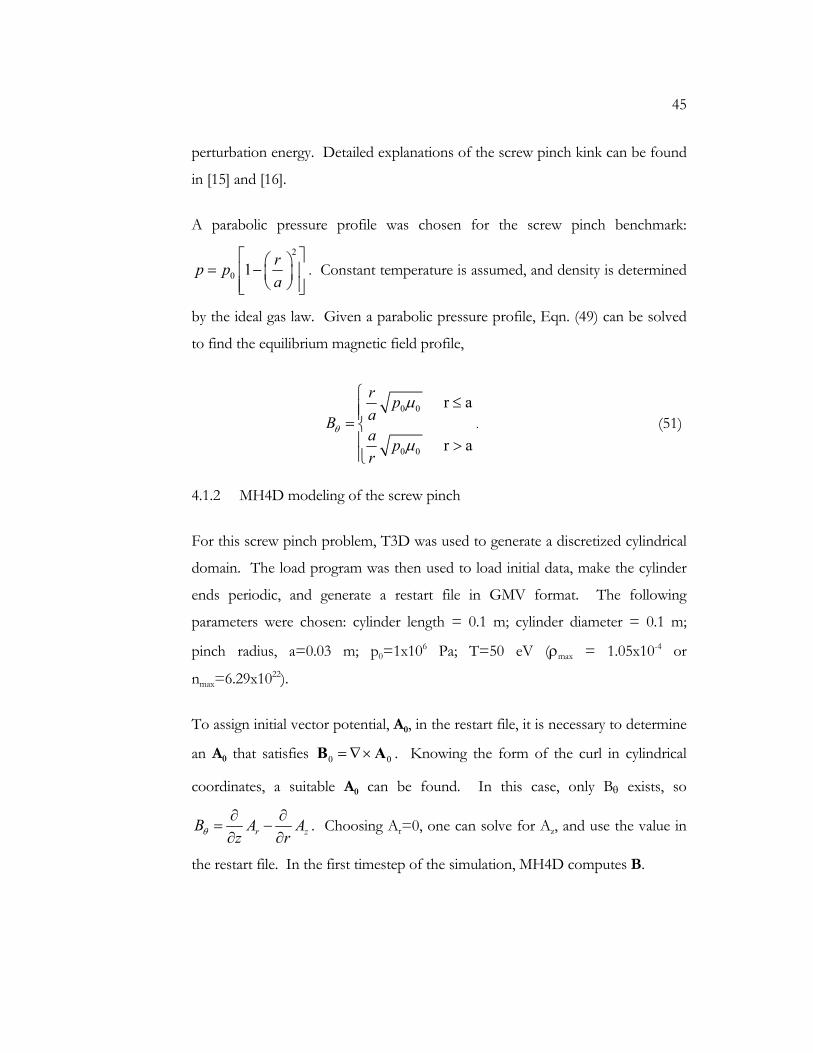
As shown in Figure 14, convergence is approximately linear with resolution as
expected for MH4D.
q Linstab
γτA
MH4D
γτA
% difference
0.5 2.514 2.464 -2.0
0.7 2.575 2.493 -3.2
0.9 2.520 2.410 -4.4
47
Figure 14: MH4D normalized kinetic energy growth rate predictions vs. resolution. Peak resolution is 2 mm (a/dx=15) which required a total of 350,000 tetrahedra.
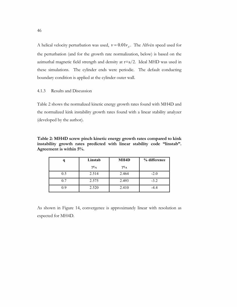
Figure 15 shows the kinetic energy evolution of an MH4D simulation. Notice
the clear linear behavior beginning at about 0.5 µsec.
Figure 15: MH4D screw pinch kinetic energy vs. time (dx=5 mm).
y = -75.717x + 2.464
y = -100.88x + 2.4932
y = -128.38x + 2.4102
1.61.71.81.92.02.12.22.32.42.52.6
0.000 0.001 0.002 0.003 0.004 0.005 0.006
dx, meters
γτA
MH4D, q=0.5MH4D, q=0.7MH4D, q=0.9
48
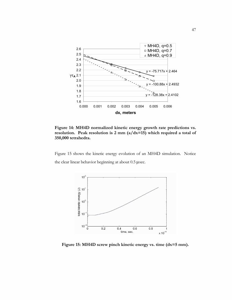
Figure 16: MH4D screw pinch simulation snapshot showing pressure contours. t=0.9 µs (dx=5 mm). For reference, 0.5 sAτ µ≈ .
A snapshot of a kinking screw pinch is shown in Figure 16.
As seen in Figure 14, the highest resolution used is 2 mm. With this resolution,
there are 15 grid cells across the pinch radius. Higher resolutions are possible,
but would not likely alter the conclusions that can be drawn. MH4D simulations
agree with linear stability analysis within 5%, and build confidence that MH4D
properly captures magnetohydrodynamic plasma behavior. The cause of the 5%
discrepancy is not known with certainty. A possible explanation is that non-linear
effects are present by the time clear linear growth is present in the simulations.
4.2 Spheromak
In a second linear stability test, the m=1 tilt mode of a spheromak in a “tuna can”
cylindrical domain was simulated and compared to published growth rate
calculations. This test was performed for two main reasons. First, due to the
49
discrepancy between MH4D screw pinch kink mode growth rate predictions and
linear stability analyzer predictions, a second benchmark was desirable. Second,
the PSI-Center had previously used spheromak tilt mode simulations to test
atomic physics models. Developing spheromak tilt simulations in MH4D
provided continuity between MH4D atomic physics development and previous
atomic physics work.
4.2.1 Theoretical Background
Details about spheromak equilibria can be found in Bellan [12]. The three
components of magnetic field for an m=0 cylindrical equilibrium are as follows:
( ) ( )
( ) ( )
( ) ( )
0 1
2
0 12
0 0
cos
1 sin
sin
zr r z
r
zr z
r
z r z
kB B J k r k zk
kB B J k r k zk
B B J k r k z
φ
= −
= +
=
(52)
where kz=π/L, kr=3.8317/R, and L and R are the length and radius of the
cylindrical domain.
Two spheromaks are shown in Figure 17. On the left is a stable spheromak in an
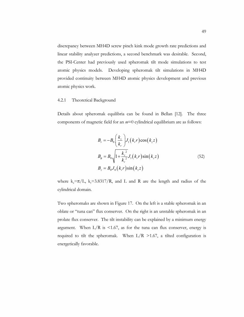
oblate or “tuna can” flux conserver. On the right is an unstable spheromak in an
prolate flux conserver. The tilt instability can be explained by a minimum energy
argument. When L/R is <1.67, as for the tuna can flux conserver, energy is
required to tilt the spheromak. When L/R >1.67, a tilted configuration is
energetically favorable.
50
⇒L
R
⇒⇒⇒L
R
Figure 17: Illustrations of tilt-stable (left) and tilt-unstable (right) spheromak configurations.
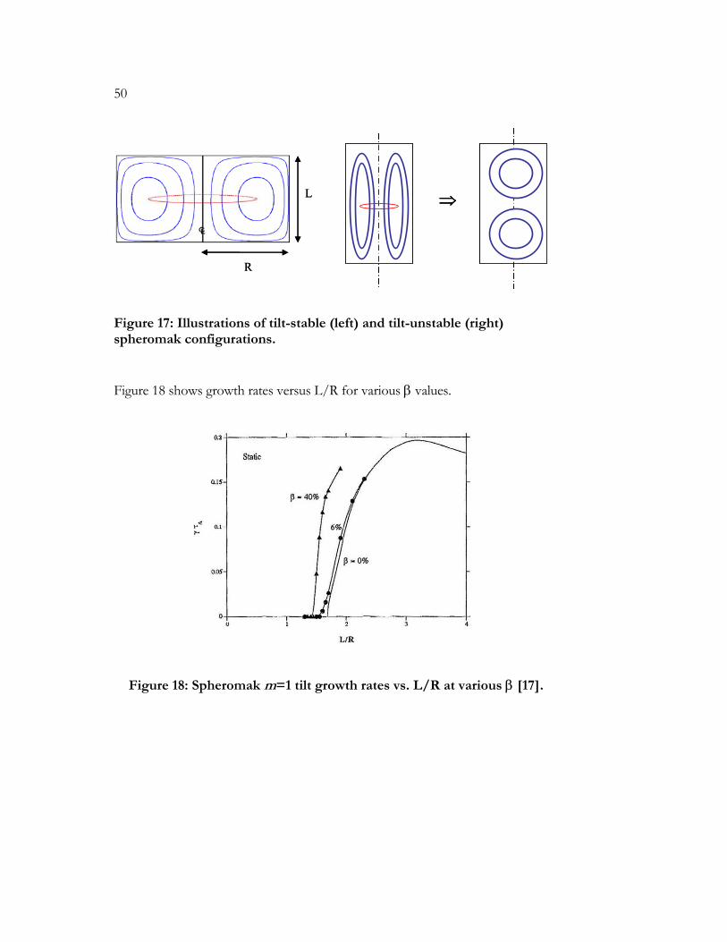
Figure 18 shows growth rates versus L/R for various β values.
Figure 18: Spheromak m=1 tilt growth rates vs. L/R at various β [17].
51
4.2.2 MH4D modeling of the spheromak
Initially, the plasma has uniform pressure=100 Pa and temperature=10 eV. The
initial magnetic field peaks at 1 T, and corresponds to the zero-β equilibrium field
per Eqn. (52). Thus, the initial plasma β is 0.025%7. L/R=2.5 was chosen for
these simulations, where L=2.5 m and R=1 m.
In MH4D, the initial condition must be provided in terms of A (MH4D’s
primitive variable) rather than B. For this axisymmetric configuration, we know
that
( )
( )
( ) ( )1
rr
r z
zz
Az
A Az r
rAr r
φ
φφ
φ
∂∇× = = −
∂∂ ∂
∇× = = −∂ ∂
∂∇× = =
∂
A B
A B
A B
(53)
Solving the upper equation of Eqns. (53), rz
A B dzφ = −∫ . One of the two
remaining components, Ar and Az, can be assumed equal to zero. Taking Az=0,
straightforward integration yields a form for A whose curl is the desired B.
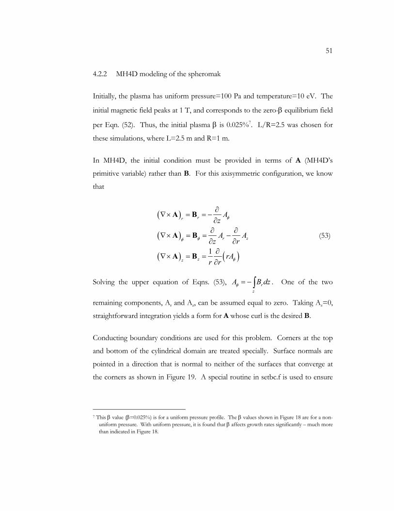
Conducting boundary conditions are used for this problem. Corners at the top
and bottom of the cylindrical domain are treated specially. Surface normals are
pointed in a direction that is normal to neither of the surfaces that converge at
the corners as shown in Figure 19. A special routine in setbc.f is used to ensure
7 This β value (β=0.025%) is for a uniform pressure profile. The β values shown in Figure 18 are for a non-
uniform pressure. With uniform pressure, it is found that β affects growth rates significantly – much more than indicated in Figure 18.
52
that appropriate normal or tangential components are zeroed on both converging
surfaces.
n
Figure 19: Incorrect surface normal at corner of cylindrical spheromak domain.
Tangential boundary components of A, determined from Eqns. (53), are non-
zero. With some slight code modifications, MH4D handles this naturally by
requiring tang. 0t
∂=
∂
A instead of tang. 0=A on conducting boundaries.
The perturbation for the problem is a rigid rotor velocity perturbation modulated
by parabolic functions of radius and height to prevent perturbed velocity at radial
and axial boundaries. The rotation is around an axis perpendicular to the cylinder
centerline through the geometric center of the cylinder. The perturbation value is
0.001 Av v= . The Alfvén speed used for this perturbation (and for growth rate
normalization, below) is based on the peak magnetic field strength and the
uniform initial plasma density.
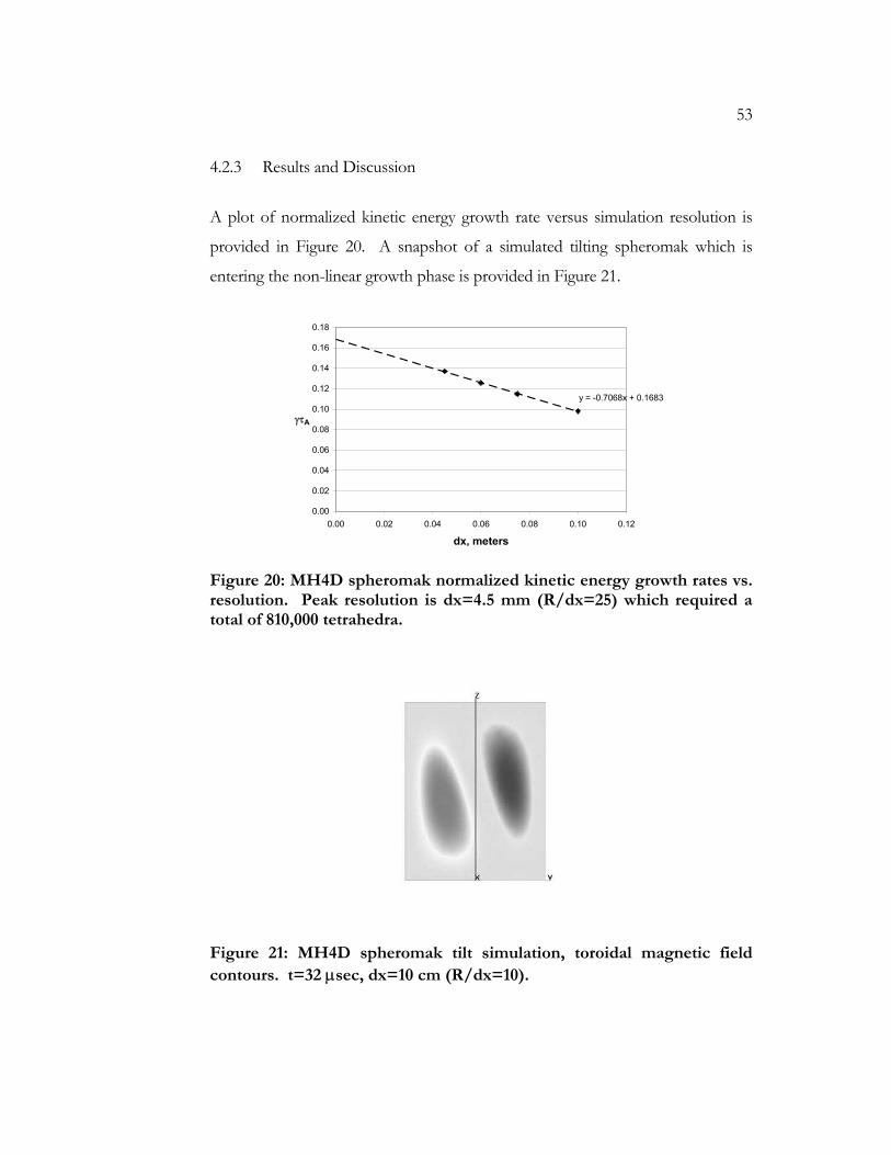
53
4.2.3 Results and Discussion
A plot of normalized kinetic energy growth rate versus simulation resolution is
provided in Figure 20. A snapshot of a simulated tilting spheromak which is
entering the non-linear growth phase is provided in Figure 21.
y = -0.7068x + 0.1683
0.00
0.02
0.04
0.06
0.08
0.10
0.12
0.14
0.16
0.18
0.00 0.02 0.04 0.06 0.08 0.10 0.12
dx, meters
γτA
Figure 20: MH4D spheromak normalized kinetic energy growth rates vs. resolution. Peak resolution is dx=4.5 mm (R/dx=25) which required a total of 810,000 tetrahedra.
Figure 21: MH4D spheromak tilt simulation, toroidal magnetic field contours. t=32 µsec, dx=10 cm (R/dx=10).
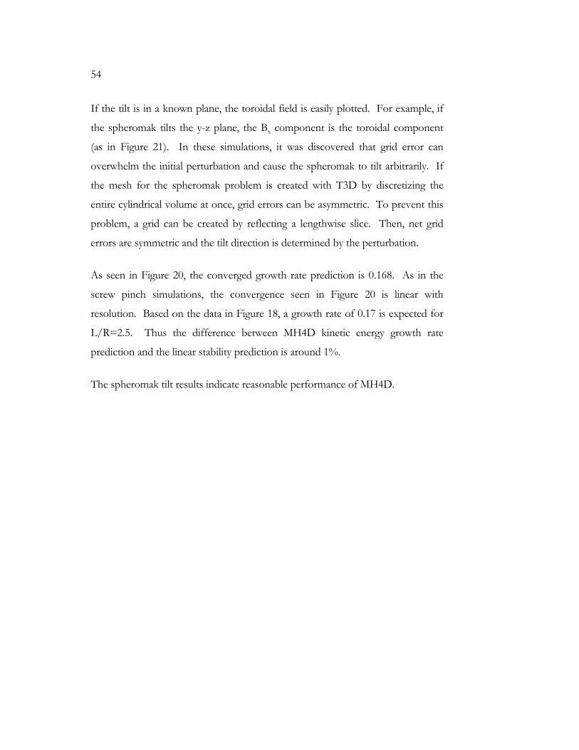
54
If the tilt is in a known plane, the toroidal field is easily plotted. For example, if
the spheromak tilts the y-z plane, the Bx component is the toroidal component
(as in Figure 21). In these simulations, it was discovered that grid error can
overwhelm the initial perturbation and cause the spheromak to tilt arbitrarily. If
the mesh for the spheromak problem is created with T3D by discretizing the
entire cylindrical volume at once, grid errors can be asymmetric. To prevent this
problem, a grid can be created by reflecting a lengthwise slice. Then, net grid
errors are symmetric and the tilt direction is determined by the perturbation.
As seen in Figure 20, the converged growth rate prediction is 0.168. As in the
screw pinch simulations, the convergence seen in Figure 20 is linear with
resolution. Based on the data in Figure 18, a growth rate of 0.17 is expected for
L/R=2.5. Thus the difference between MH4D kinetic energy growth rate
prediction and the linear stability prediction is around 1%.
The spheromak tilt results indicate reasonable performance of MH4D.
55
Chapter 5
ATOMIC PHYSICS TESTS
5.1 Simulation of stationary, constant temperature plasma
Three test problems involving stationary, constant temperature plasma have been
solved. Two of the problems have analytical solutions. The third problem is a
coronal equilibrium test for which empirical results are available in literature. The
test problems and results are presented, and then implementation details are
discussed.
5.1.1 Background for analytical test problems
With the ionization and recombination models described in Section 3.5, two
simple problems with analytical solutions have been solved with MH4D. In these
problems, the plasma has zero velocity, and temperature is constant. A spatially
and temporally constant neutral density is assumed. A box domain with coarse
discretization (roughly 100 tetrahedra) is used. Conducting hardwall boundary
conditions are used.
The equation describing ionization is
iion e i nnt
ρ σ ρ∂= ⟨ ⟩
∂v ,
which has the analytical solution,
( ) [ ]0 expi ion et tρ ρ σ= ⟨ ⟩v ,
where ρ0 is the initial plasma density. For recombination,
56
2irec e i i rec e in C
tρ σ ρ σ ρ∂
= −⟨ ⟩ = −⟨ ⟩∂
v v ,
where C is the conversion from kg/m3 to #/m3. This has the solution,
1
0
1i ion et Cρ σ
ρ
−
= ⟨ ⟩ +
v .
These two analytical problems are called the “isolated ionization” and “isolated
recombination” problems.
5.1.2 Background for coronal equilibrium test problem
At a given temperature, the ionization fraction of a plasma in coronal equilibrium
is predictable. A variable neutral density is implemented in MH4D to allow this
test.
5.1.3 Results and discussion
MH4D successfully produces the analytical solutions for various initial data and
ionization and recombination rates for the isolated ionization and isolated
recombination problems. Some difficulty was encountered with timestep choice
in the isolated ionization problem. Consider the number density change for
plasma, iion e i n
n n nt
σ∂= ⟨ ⟩
∂v . MH4D is set up so that the number of new ions
cannot exceed the number of available neutrals. Thus, if in tt
∂∆
∂ exceeds nn , the
solution found by MH4D does not match the analytical solution (this is obvious
in retrospect).
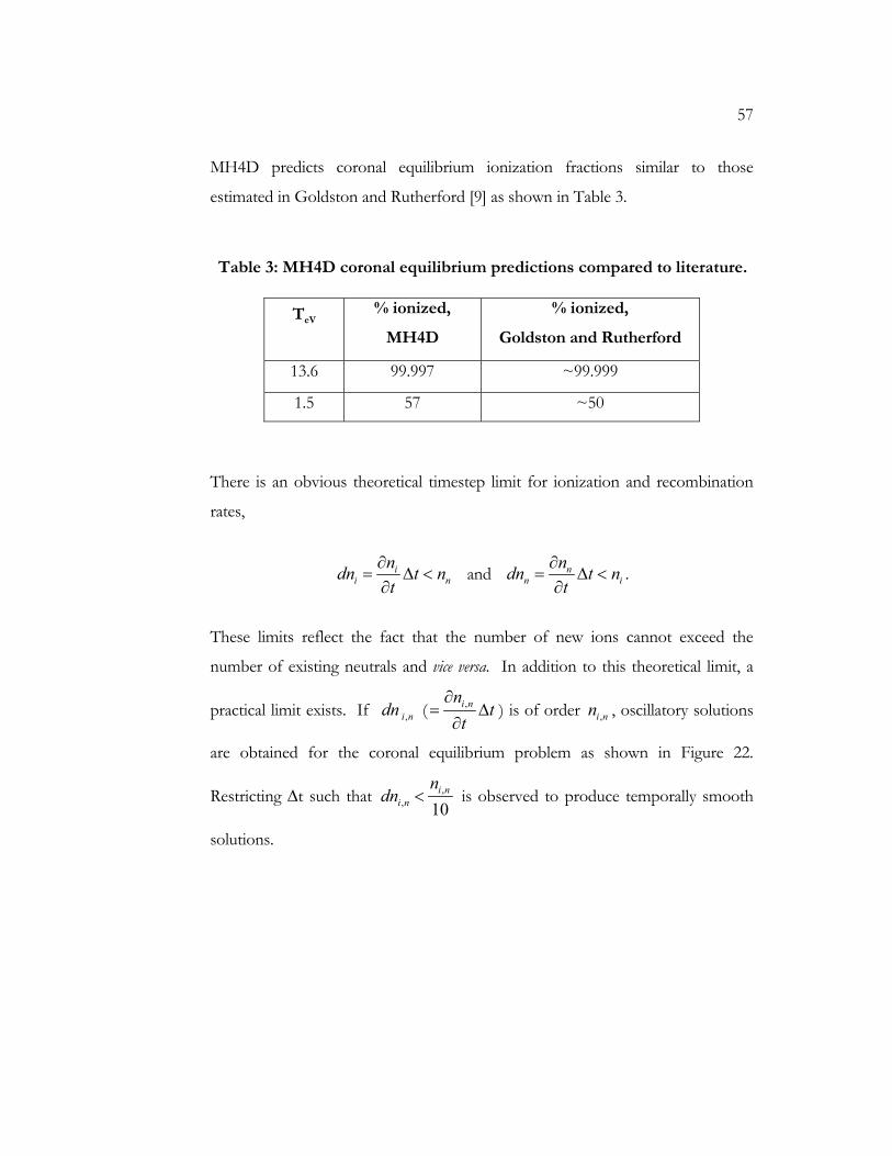
57
MH4D predicts coronal equilibrium ionization fractions similar to those
estimated in Goldston and Rutherford [9] as shown in Table 3.
Table 3: MH4D coronal equilibrium predictions compared to literature.
TeV % ionized,
MH4D
% ionized,
Goldston and Rutherford
13.6 99.997 ~99.999
1.5 57 ~50
There is an obvious theoretical timestep limit for ionization and recombination
rates,
ii n
ndn t nt
∂= ∆ <
∂ and n
n indn t nt
∂= ∆ <
∂.
These limits reflect the fact that the number of new ions cannot exceed the
number of existing neutrals and vice versa. In addition to this theoretical limit, a
practical limit exists. If ,i ndn ( ,i nn tt
∂= ∆
∂) is of order ,i nn , oscillatory solutions
are obtained for the coronal equilibrium problem as shown in Figure 22.
Restricting ∆t such that ,, 10
i ni n
ndn < is observed to produce temporally smooth
solutions.
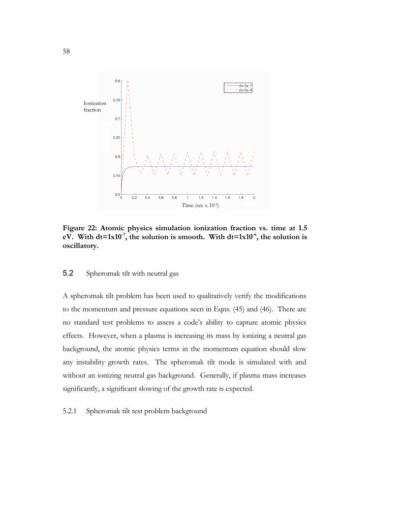
58
Figure 22: Atomic physics simulation ionization fraction vs. time at 1.5 eV. With dt=1x10⁻⁷, the solution is smooth. With dt=1x10⁻⁶, the solution is oscillatory.
5.2 Spheromak tilt with neutral gas
A spheromak tilt problem has been used to qualitatively verify the modifications
to the momentum and pressure equations seen in Eqns. (45) and (46). There are
no standard test problems to assess a code’s ability to capture atomic physics
effects. However, when a plasma is increasing its mass by ionizing a neutral gas
background, the atomic physics terms in the momentum equation should slow
any instability growth rates. The spheromak tilt mode is simulated with and
without an ionizing neutral gas background. Generally, if plasma mass increases
significantly, a significant slowing of the growth rate is expected.
5.2.1 Spheromak tilt test problem background
Time (sec x 10-5)
Ionization fraction
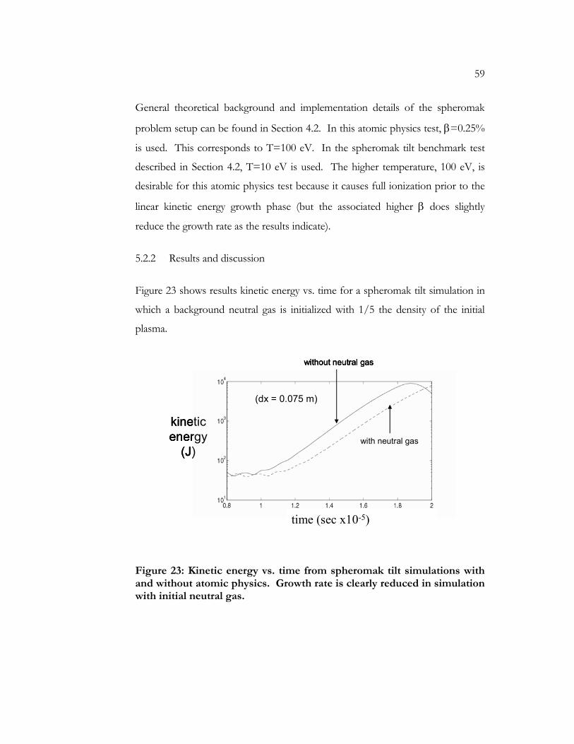
59
General theoretical background and implementation details of the spheromak
problem setup can be found in Section 4.2. In this atomic physics test, β=0.25%
is used. This corresponds to T=100 eV. In the spheromak tilt benchmark test
described in Section 4.2, T=10 eV is used. The higher temperature, 100 eV, is
desirable for this atomic physics test because it causes full ionization prior to the
linear kinetic energy growth phase (but the associated higher β does slightly
reduce the growth rate as the results indicate).
5.2.2 Results and discussion
Figure 23 shows results kinetic energy vs. time for a spheromak tilt simulation in
which a background neutral gas is initialized with 1/5 the density of the initial
plasma.
kineticenergy
(J)with neutral gas
without neutral gas
time (sec x10-5)
(dx = 0.075 m)
kineticenergy
(J)with neutral gas
without neutral gas
time (sec x10-5)
kineticenergy
(J)with neutral gas
without neutral gas
time (sec x10-5)
(dx = 0.075 m)
Figure 23: Kinetic energy vs. time from spheromak tilt simulations with and without atomic physics. Growth rate is clearly reduced in simulation with initial neutral gas.
60
Figure 24 shows how the total plasma mass varies with time. As seen, the neutral
gas is quickly and nearly completely ionized. The increased mass slows the
spheromak tilt as seen in Figure 23. The converged tilt growth rate without
neutral gas is found to be 0.161. With an initial neutral gas background, the
growth rate is 0.146 – reduced by 9%. This result qualitatively verifies the atomic
physics implementation.
( )( 0)
plasma
plasma
m tm t =
( )time s
Figure 24: Total plasma mass as a fraction of initial mass vs. simulation time for spheromak with initial neutral gas. The plasma is fully ionized by 10 µs.
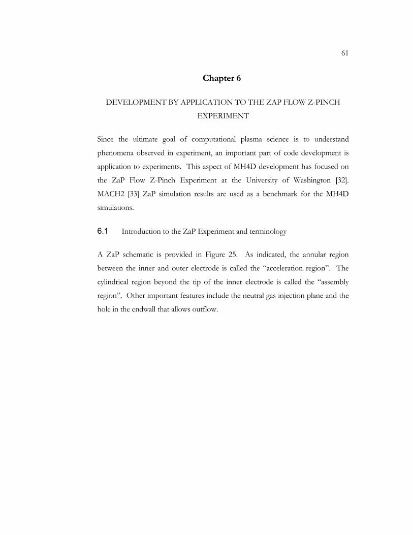
61
Chapter 6
DEVELOPMENT BY APPLICATION TO THE ZAP FLOW Z-PINCH
EXPERIMENT
Since the ultimate goal of computational plasma science is to understand
phenomena observed in experiment, an important part of code development is
application to experiments. This aspect of MH4D development has focused on
the ZaP Flow Z-Pinch Experiment at the University of Washington [32].
MACH2 [33] ZaP simulation results are used as a benchmark for the MH4D
simulations.
6.1 Introduction to the ZaP Experiment and terminology
A ZaP schematic is provided in Figure 25. As indicated, the annular region
between the inner and outer electrode is called the “acceleration region”. The
cylindrical region beyond the tip of the inner electrode is called the “assembly
region”. Other important features include the neutral gas injection plane and the
hole in the endwall that allows outflow.
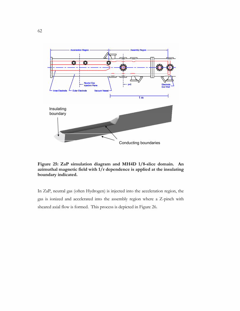
62
Insulatingboundary
Conducting boundaries
Figure 25: ZaP simulation diagram and MH4D 1/8-slice domain. An azimuthal magnetic field with 1/r dependence is applied at the insulating boundary indicated.
In ZaP, neutral gas (often Hydrogen) is injected into the acceleration region, the
gas is ionized and accelerated into the assembly region where a Z-pinch with
sheared axial flow is formed. This process is depicted in Figure 26.
63
Figure 26: Conceptual diagrams of ZaP Z-pinch formation [34]. In the upper frame, an annular current sheet has developed and a “snowplow” effect is seen. In the lower frame, the Z-pinch formation has started and residual neutral gas and plasma is present in the acceleration region.
While the neutral gas is still concentrated near the ports, voltage is applied and
some of the gas is ionized. This ionized gas forms an annular current sheet which
is accelerated axially into the assembly region by Lorentz forces. Near the inner
electrode, higher current density and higher magnetic fields cause a “snowplow”
effect in which plasma close to the inner electrode moves faster than outer
plasma. The sheet is stretched as it forms the Z-pinch, embedding axially sheared
flow in the pinch. Some residual plasma is left behind in the acceleration region.
New plasma is formed from the neutral gas that was not initially ionized. Sheared
64
flow is probably maintained to some extent by plasma that emerges from the
acceleration region well after initial pinch formation. Sheared flow stabilizes the
Z-pinch for over 2000 times the growth time of a static Z-pinch [32]. Resolved
MHD simulations of ZaP should capture the essential behavior described above.
6.2 Basic ZaP simulation approach
1-eV plasma is initialized in an annular volume with 20 cm axial length, centered
on the neutral gas injection plane in the acceleration region. The initial plasma
density is 6.0x10⁻⁵ kg/m3, corresponding to a total mass of 2.8x10⁻⁷ kg. Total
mass injected in the experiment is typically 1-3x10⁻⁷ kg.
Flux is injected at the insulating boundary shown in Figure 258. To accomplish
the flux injection, a time-varying magnetic field boundary condition is applied to
the insulating back wall. The applied field is in the azimuthal direction. The
current generated due to the applied field can be calculated using Ampère’s Law:
( )0 / 2encB I rθ µ π= . (Refer to Figure 28 for current profiles used in simulations.)
Except for the insulator, boundaries are modeled as conducting walls. To make
high-resolution simulations feasible, periodic boundary conditions are used to
model only a 1/8-slice of the domain. Various combinations of Chodura and
Spitzer resistivity are used. Sometimes, a resistivity floor is used to maintain
dissipation in the simulations. A resistivity cap is always used to prevent extreme
numerical stiffness. A density floor is used with a value 10 to 100 times smaller
than the initial density in the gas puff.
8 Treating the entire back wall of the experiment as an insulating boundary is a simplification, but modeling
the more complicated insulator geometry should not significantly change the simulation results.
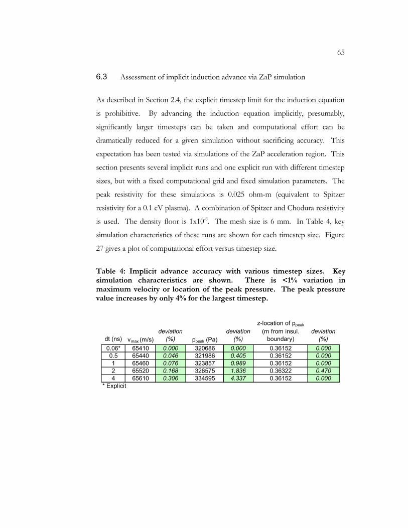
65
6.3 Assessment of implicit induction advance via ZaP simulation
As described in Section 2.4, the explicit timestep limit for the induction equation
is prohibitive. By advancing the induction equation implicitly, presumably,
significantly larger timesteps can be taken and computational effort can be
dramatically reduced for a given simulation without sacrificing accuracy. This
expectation has been tested via simulations of the ZaP acceleration region. This
section presents several implicit runs and one explicit run with different timestep
sizes, but with a fixed computational grid and fixed simulation parameters. The
peak resistivity for these simulations is 0.025 ohm-m (equivalent to Spitzer
resistivity for a 0.1 eV plasma). A combination of Spitzer and Chodura resistivity
is used. The density floor is 1x10⁻⁶. The mesh size is 6 mm. In Table 4, key
simulation characteristics of these runs are shown for each timestep size. Figure
27 gives a plot of computational effort versus timestep size.
Table 4: Implicit advance accuracy with various timestep sizes. Key simulation characteristics are shown. There is <1% variation in maximum velocity or location of the peak pressure. The peak pressure value increases by only 4% for the largest timestep.
dt (ns) vmax (m/s)deviation
(%) ppeak (Pa)deviation
(%)
z-location of ppeak
(m from insul. boundary)
deviation (%)
0.06* 65410 0.000 320686 0.000 0.36152 0.0000.5 65440 0.046 321986 0.405 0.36152 0.0001 65460 0.076 323857 0.989 0.36152 0.0002 65520 0.168 326575 1.836 0.36322 0.4704 65610 0.306 334595 4.337 0.36152 0.000
* Explicit
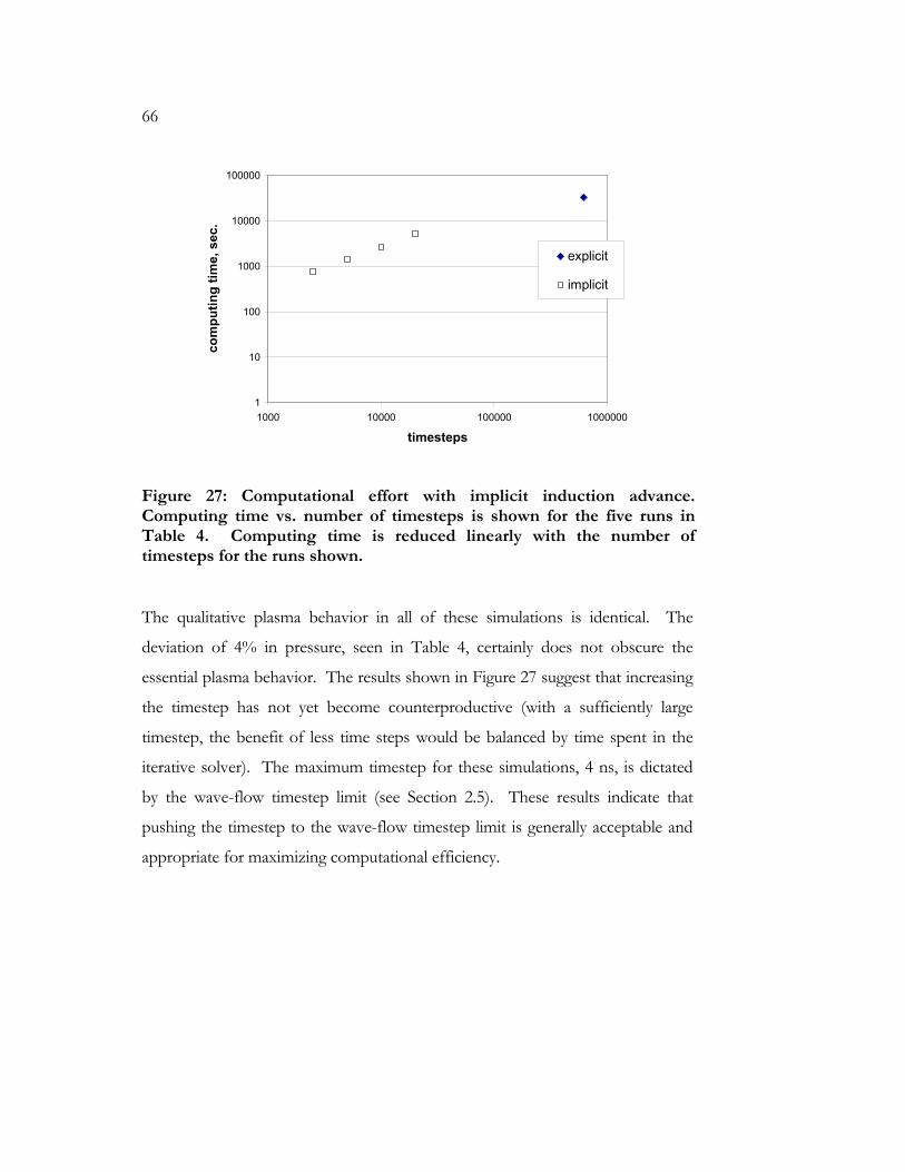
66
1
10
100
1000
10000
100000
1000 10000 100000 1000000
timesteps
com
putin
g tim
e, s
ec.
explicit
implicit
Figure 27: Computational effort with implicit induction advance. Computing time vs. number of timesteps is shown for the five runs in Table 4. Computing time is reduced linearly with the number of timesteps for the runs shown.
The qualitative plasma behavior in all of these simulations is identical. The
deviation of 4% in pressure, seen in Table 4, certainly does not obscure the
essential plasma behavior. The results shown in Figure 27 suggest that increasing
the timestep has not yet become counterproductive (with a sufficiently large
timestep, the benefit of less time steps would be balanced by time spent in the
iterative solver). The maximum timestep for these simulations, 4 ns, is dictated
by the wave-flow timestep limit (see Section 2.5). These results indicate that
pushing the timestep to the wave-flow timestep limit is generally acceptable and
appropriate for maximizing computational efficiency.

67
6.4 MACH2 benchmark
MH4D ZaP simulations have been performed. The results are benchmarked
against ZaP simulation results from MACH2 [33], a 2½D MHD code. The
MACH2 simulations were not conducted as part of this research.
In Section 6.4.1, MACH2 and MH4D simulation conditions are compared.
Sections 6.4.2 and 6.4.3 present MACH2 and MH4D results. In Section 6.4.4,
results are compared and discussed.
6.4.1 Simulation conditions
Simulation conditions for MACH2 and MH4D are shown in Table 5. In ZaP, a
hole in the endwall allows outflow. This outflow boundary is modeled in
MACH2 but not in MH4D. The resolutions used in the MH4D runs are
significantly lower than the corresponding resolutions in MACH2 runs.
Differences in density floor and radiation modeling are probably of secondary
importance as compared to the outflow boundary condition and the resolution
difference.
The current profiles for MH4D and MACH2 are similar as shown in Figure 28.
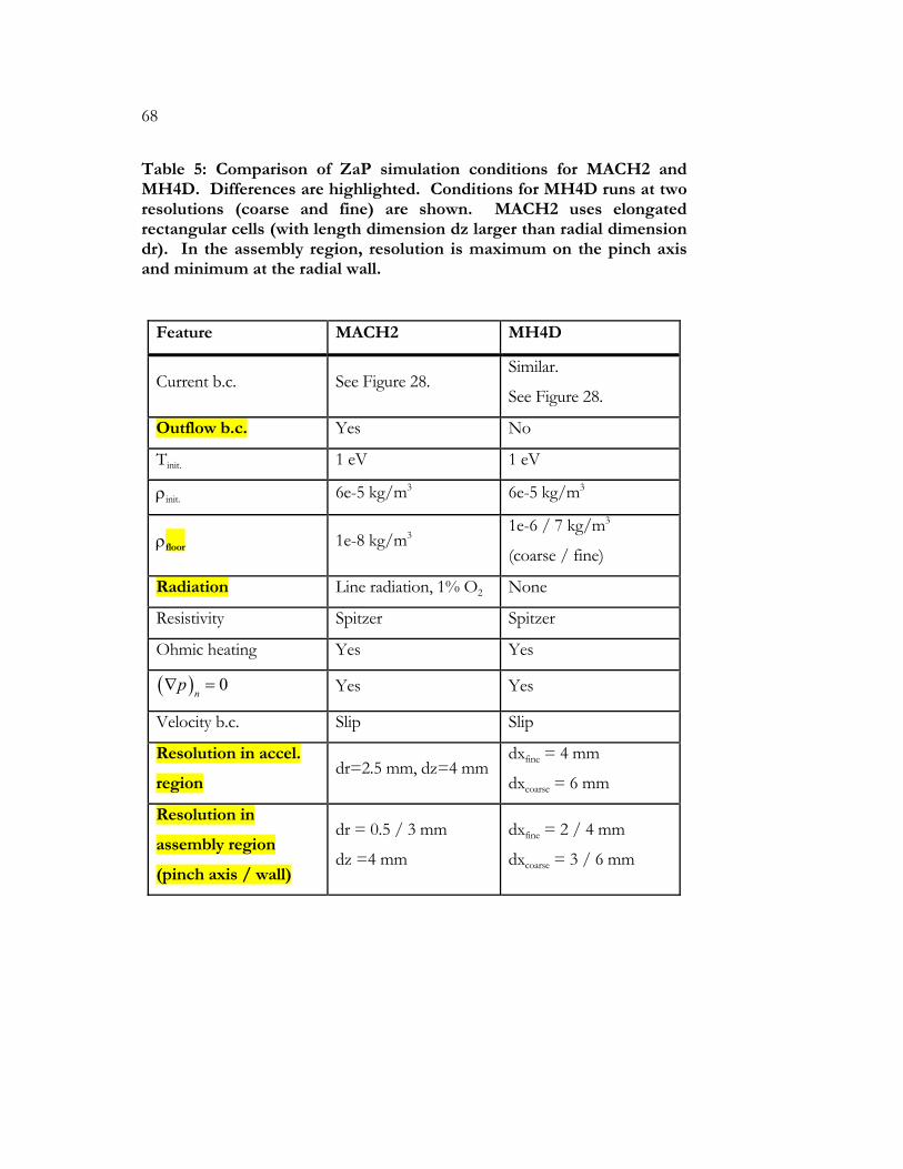
68
Table 5: Comparison of ZaP simulation conditions for MACH2 and MH4D. Differences are highlighted. Conditions for MH4D runs at two resolutions (coarse and fine) are shown. MACH2 uses elongated rectangular cells (with length dimension dz larger than radial dimension dr). In the assembly region, resolution is maximum on the pinch axis and minimum at the radial wall.
Feature MACH2 MH4D
Current b.c. See Figure 28. Similar.
See Figure 28.
Outflow b.c. Yes No
Tinit. 1 eV 1 eV
ρinit. 6e-5 kg/m3 6e-5 kg/m3
ρfloor 1e-8 kg/m3 1e-6 / 7 kg/m3
(coarse / fine)
Radiation Line radiation, 1% O2 None
Resistivity Spitzer Spitzer
Ohmic heating Yes Yes
( ) 0n
p∇ = Yes Yes
Velocity b.c. Slip Slip
Resolution in accel.
region dr=2.5 mm, dz=4 mm
dxfine = 4 mm
dxcoarse = 6 mm
Resolution in
assembly region
(pinch axis / wall)
dr = 0.5 / 3 mm
dz =4 mm
dxfine = 2 / 4 mm
dxcoarse = 3 / 6 mm
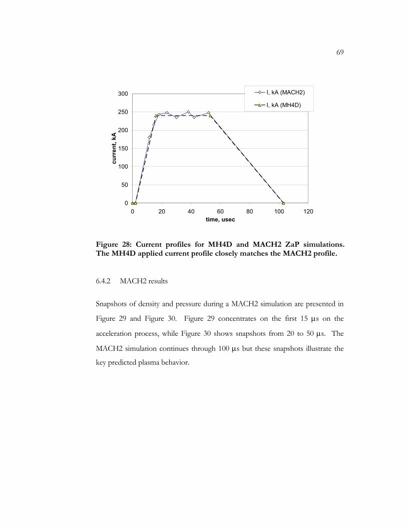
69
0
50
100
150
200
250
300
0 20 40 60 80 100 120time, usec
curr
ent,
kA
I, kA (MACH2)
I, kA (MH4D)
Figure 28: Current profiles for MH4D and MACH2 ZaP simulations. The MH4D applied current profile closely matches the MACH2 profile.
6.4.2 MACH2 results
Snapshots of density and pressure during a MACH2 simulation are presented in
Figure 29 and Figure 30. Figure 29 concentrates on the first 15 µs on the
acceleration process, while Figure 30 shows snapshots from 20 to 50 µs. The
MACH2 simulation continues through 100 µs but these snapshots illustrate the
key predicted plasma behavior.
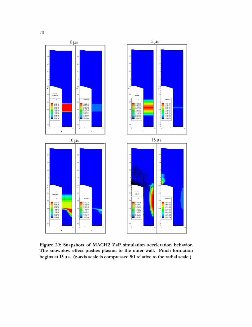
70
Figure 29: Snapshots of MACH2 ZaP simulation acceleration behavior. The snowplow effect pushes plasma to the outer wall. Pinch formation begins at 15 µs. (z-axis scale is compressed 5:1 relative to the radial scale.)
0 µs 5 µs
10 µs 15 µs
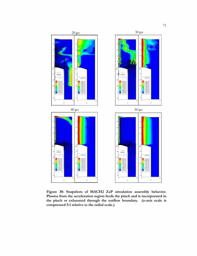
71
Figure 30: Snapshots of MACH2 ZaP simulation assembly behavior. Plasma from the acceleration region feeds the pinch and is incorporated in the pinch or exhausted through the outflow boundary. (z-axis scale is compressed 5:1 relative to the radial scale.)
20 µs 30 µs
40 µs 50 µs

72
6.4.3 MH4D results
Two MH4D simulations are presented. Parameters for the simulations are
shown in Table 5. One is called the “coarse” simulation and the other, “fine”.
The coarse simulation has 420,000 tetrahedra and the fine simulation has
1,300,000 tetrahedra. The differences in the simulations are in resolution and
density floor: in the “fine” run, mesh size 50% smaller, and the density floor is
lower by a factor of 10. Snapshots corresponding to the snapshots presented for
MACH2 are presented in Figure 31 and Figure 32 for the coarse run and Figure
33 and Figure 34 for the fine run.
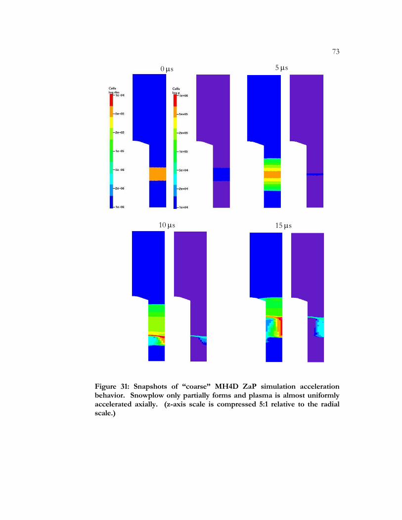
73
Figure 31: Snapshots of “coarse” MH4D ZaP simulation acceleration behavior. Snowplow only partially forms and plasma is almost uniformly accelerated axially. (z-axis scale is compressed 5:1 relative to the radial scale.)
0 µs 5 µs
10 µs 15 µs
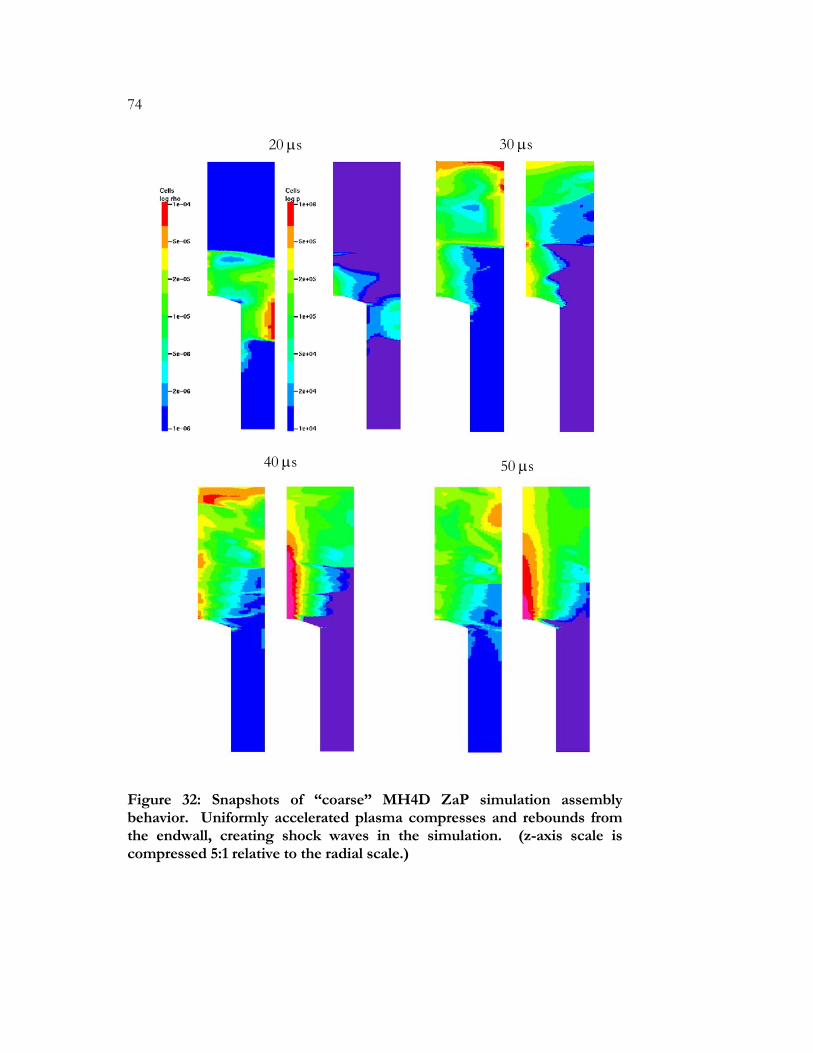
74
Figure 32: Snapshots of “coarse” MH4D ZaP simulation assembly behavior. Uniformly accelerated plasma compresses and rebounds from the endwall, creating shock waves in the simulation. (z-axis scale is compressed 5:1 relative to the radial scale.)
20 µs 30 µs
40 µs 50 µs
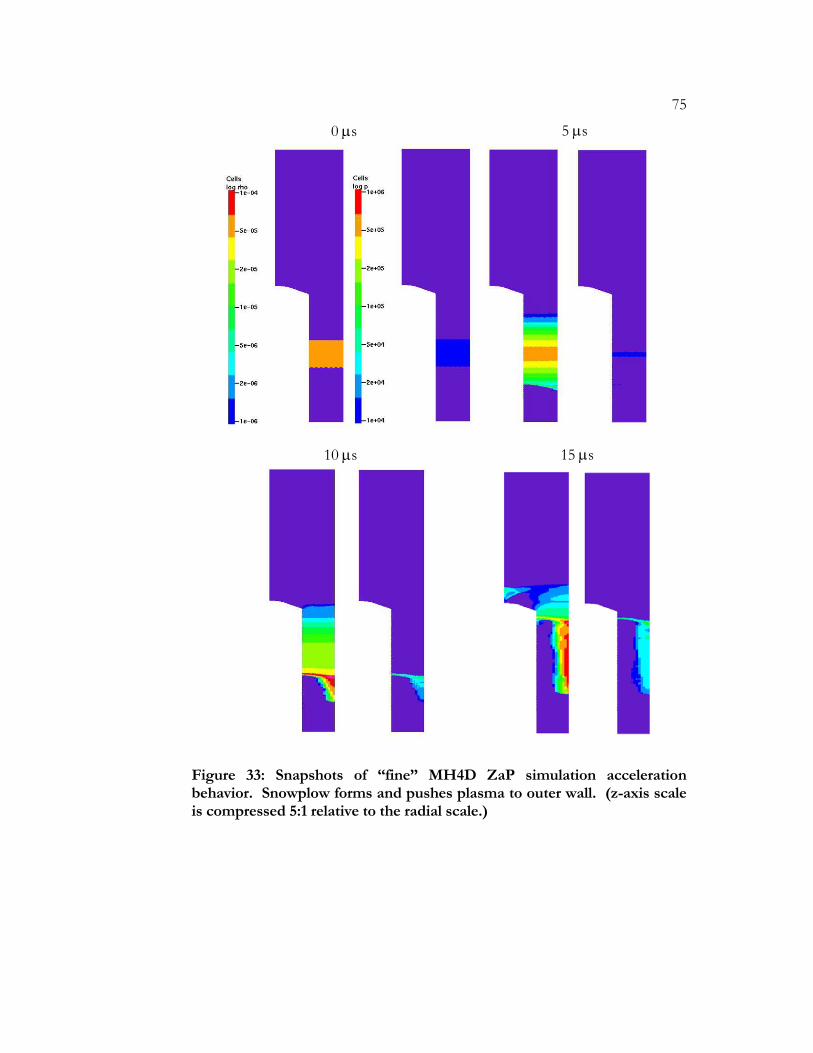
75
Figure 33: Snapshots of “fine” MH4D ZaP simulation acceleration behavior. Snowplow forms and pushes plasma to outer wall. (z-axis scale is compressed 5:1 relative to the radial scale.)
0 µs 5 µs
10 µs 15 µs
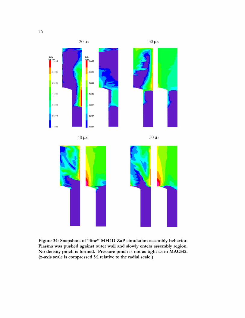
76
Figure 34: Snapshots of “fine” MH4D ZaP simulation assembly behavior. Plasma was pushed against outer wall and slowly enters assembly region. No density pinch is formed. Pressure pinch is not as tight as in MACH2. (z-axis scale is compressed 5:1 relative to the radial scale.)
20 µs 30 µs
40 µs 50 µs
77
6.4.4 Comparison and discussion
The acceleration region behavior in the fine MH4D simulation is much different
than in the coarse simulation. In the coarse simulation, the plasma is accelerated
almost uniformly toward the assembly region. Inertia carries the bulk of the
plasma to the endwall where it rebounds, causing shockwaves that are not seen in
the MACH2 results or in the fine simulation results. In the fine simulation, as in
MACH2, the snowplow forces the bulk of the plasma to the outer wall where it
moves slowly toward the assembly region. Density distributions at 20 and 30 µs
in the fine simulation are comparable to those seen in the corresponding MACH2
plots.
ZaP diagnostics reveal a discrete Z-pinch with 1-cm radius. In the 30, 40 and 50
µs snapshots, MACH2 density contours show this 1-cm-radius pinch on the axis.
MH4D does not capture this peaked density in either the coarse or the fine
simulations. This difference is probably due primarily to insufficient resolution in
the pinch region. High radial gradients in pressure and density are not resolved,
and a tight pinch cannot form in the simulations. Outflow, which is modeled in
the MACH2 simulation, but not in the MH4D simulations, could also play a role.
High magnetic fields are present in the simulations at the cathode nosecone.
Increasing resolution at the nosecone reduces the maximum magnetic field
magnitudes, indicating that the high fields are at least partly due to numerical
error (see discussion of ∇ • B in Appendix A.3). A “shadowing” effect could
also contribute to these high magnetic fields, as the predominantly axially-directed
plasma passes the cathode nosecone.
The semi-implicit algorithm is not used in these simulations. Some difficulties
have been encountered in applying the algorithm. However, even with the semi-
78
implicit momentum advance functioning to eliminate the magnetosonic wave
speed timestep restriction, high flow speeds in ZaP will force small timesteps. In
MACH2, this issue is alleviated by using elongated grid cells in the direction of
high flow speeds (i.e. the axial direction), easing the timestep restriction. MH4D
cannot use this grid alignment technique because distorted tetrahedra cause
numerical inaccuracy.
Computational effort for the fine MH4D run was 10 hours on 64 NERSC Bassi
processors (1.9 GHz per processor). Using the semi-implicit algorithm, the effort
could be reduced by roughly a factor of 5, despite the high flow speeds. Based on
this information, a simulation with MACH2-like resolution seems within reach.
In summary, MH4D simulation results are seen to converge to the MACH2
results in the acceleration region. However, predictions by MH4D and MACH2
of Z-pinch behavior in the assembly region differ significantly. As discussed,
further research to develop and improve MH4D ZaP simulations is possible.
Such research would at least explore and probably extend the known capabilities
of the code.
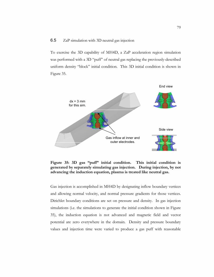
79
6.5 ZaP simulation with 3D neutral gas injection
To exercise the 3D capability of MH4D, a ZaP acceleration region simulation
was performed with a 3D “puff” of neutral gas replacing the previously-described
uniform density “block” initial condition. This 3D initial condition is shown in
Figure 35.
End view
Side view
Gas inflow at inner and outer electrodes.
dx = 3 mmfor this sim.
Figure 35: 3D gas “puff” initial condition. This initial condition is generated by separately simulating gas injection. During injection, by not advancing the induction equation, plasma is treated like neutral gas.
Gas injection is accomplished in MH4D by designating inflow boundary vertices
and allowing normal velocity, and normal pressure gradients for those vertices.
Dirichlet boundary conditions are set on pressure and density. In gas injection
simulations (i.e. the simulations to generate the initial condition shown in Figure
35), the induction equation is not advanced and magnetic field and vector
potential are zero everywhere in the domain. Density and pressure boundary
values and injection time were varied to produce a gas puff with reasonable
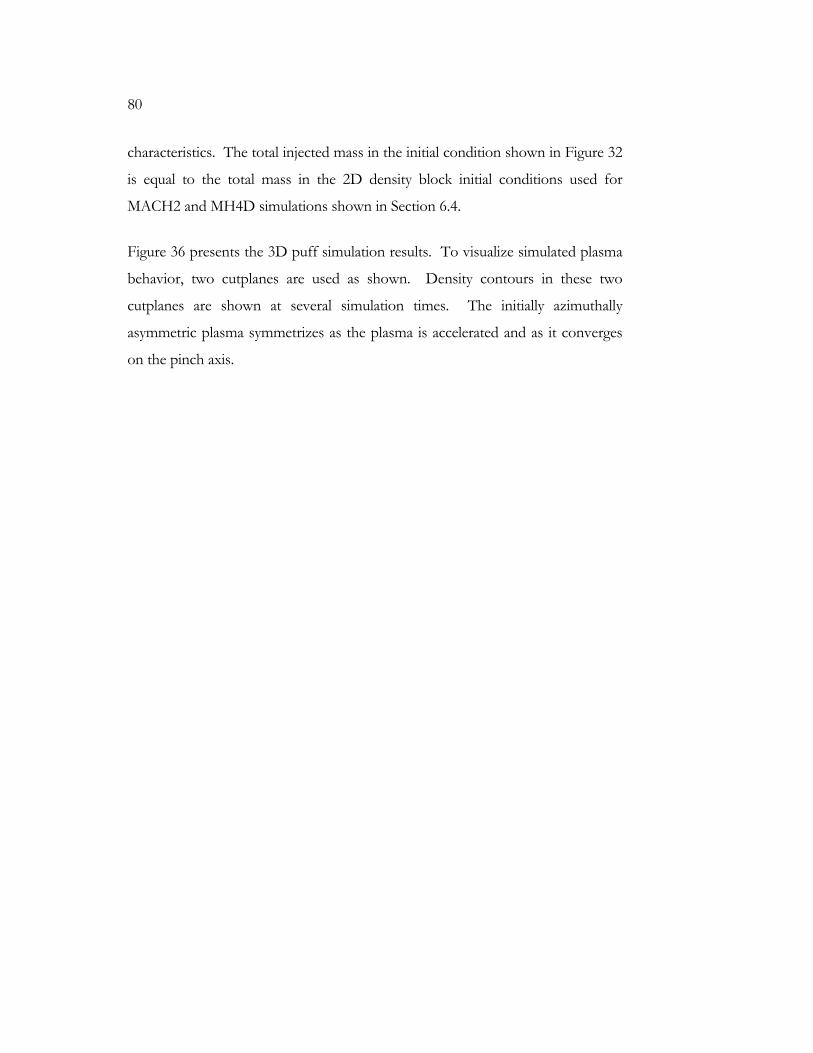
80
characteristics. The total injected mass in the initial condition shown in Figure 32
is equal to the total mass in the 2D density block initial conditions used for
MACH2 and MH4D simulations shown in Section 6.4.
Figure 36 presents the 3D puff simulation results. To visualize simulated plasma
behavior, two cutplanes are used as shown. Density contours in these two
cutplanes are shown at several simulation times. The initially azimuthally
asymmetric plasma symmetrizes as the plasma is accelerated and as it converges
on the pinch axis.
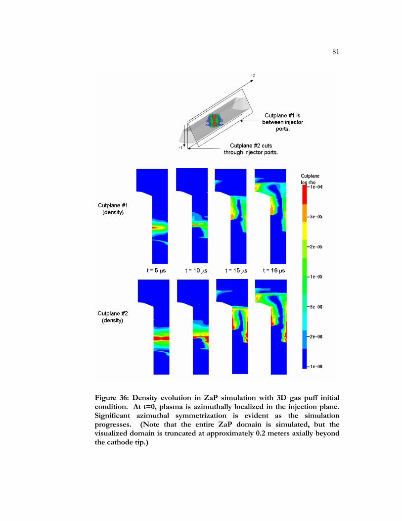
81
Figure 36: Density evolution in ZaP simulation with 3D gas puff initial condition. At t=0, plasma is azimuthally localized in the injection plane. Significant azimuthal symmetrization is evident as the simulation progresses. (Note that the entire ZaP domain is simulated, but the visualized domain is truncated at approximately 0.2 meters axially beyond the cathode tip.)
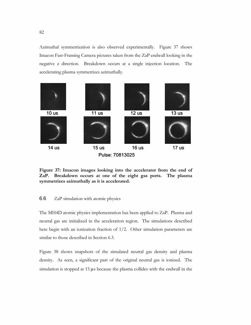
82
Azimuthal symmetrization is also observed experimentally. Figure 37 shows
Imacon Fast-Framing Camera pictures taken from the ZaP endwall looking in the
negative z direction. Breakdown occurs at a single injection location. The
accelerating plasma symmetrizes azimuthally.
10 us 11 us 12 us 13 us
14 us 15 us 16 us 17 usPulse: 70813025
10 us 11 us 12 us 13 us
14 us 15 us 16 us 17 usPulse: 70813025
Figure 37: Imacon images looking into the accelerator from the end of ZaP. Breakdown occurs at one of the eight gas ports. The plasma symmetrizes azimuthally as it is accelerated.
6.6 ZaP simulation with atomic physics
The MH4D atomic physics implementation has been applied to ZaP. Plasma and
neutral gas are initialized in the acceleration region. The simulations described
here begin with an ionization fraction of 1/2. Other simulation parameters are
similar to those described in Section 6.3.
Figure 38 shows snapshots of the simulated neutral gas density and plasma
density. As seen, a significant part of the original neutral gas is ionized. The
simulation is stopped at 15 µs because the plasma collides with the endwall in the
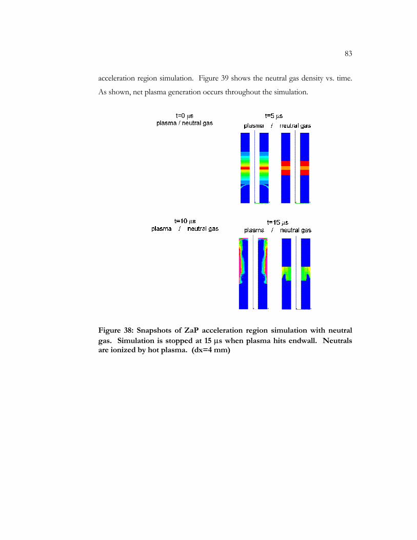
83
acceleration region simulation. Figure 39 shows the neutral gas density vs. time.
As shown, net plasma generation occurs throughout the simulation.
Figure 38: Snapshots of ZaP acceleration region simulation with neutral gas. Simulation is stopped at 15 µs when plasma hits endwall. Neutrals are ionized by hot plasma. (dx=4 mm)
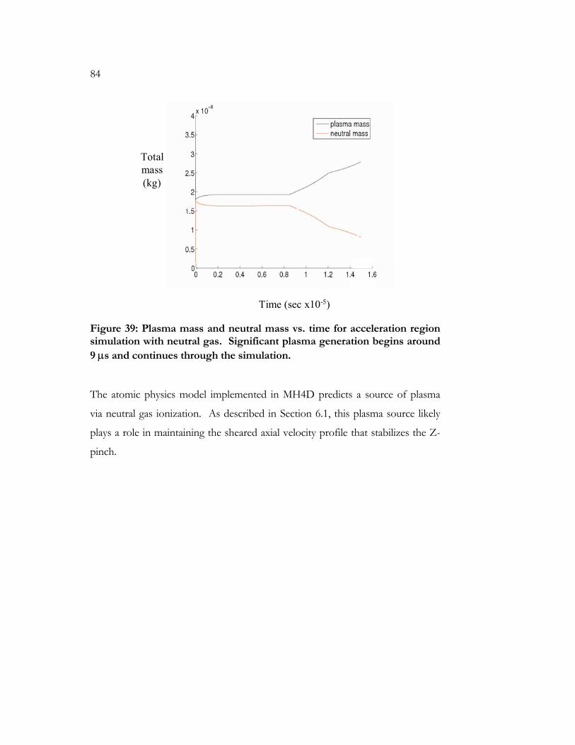
84
Totalmass(kg)
Time (sec x10-5)
Figure 39: Plasma mass and neutral mass vs. time for acceleration region simulation with neutral gas. Significant plasma generation begins around 9 µs and continues through the simulation.
The atomic physics model implemented in MH4D predicts a source of plasma
via neutral gas ionization. As described in Section 6.1, this plasma source likely
plays a role in maintaining the sheared axial velocity profile that stabilizes the Z-
pinch.
85
Chapter 7
CONCLUSION
7.1 Concluding remarks
MH4D has been improved as a computational tool by implementing useful
boundary conditions for plasma simulation, and by adding important physics
features to the code. A periodic boundary condition, useful for domain
reduction, mode selection, and wave modeling, is now available. An insulating
boundary condition has been implemented and allows flux injection. Spitzer and
Chodura resistivity models have been added, and Ohmic heating is now an
option. Atomic physics has been implemented. Simulations that have been
conducted with atomic physics provide insight into requirements for numerical
stability and accuracy, and form a basis for future development in MH4D or
other codes.
The quasi-linear regimes of the non-linear screw pinch kink and spheromak tilt
instabilities have been simulated with MH4D. The results are benchmarked
against linear stability code results, and agreement is reasonable.
MH4D is now adaptable to a variety of problems as shown in this research. In
addition to the instability simulations, the code has been applied to the ZaP Flow
Z-Pinch experiment. When resolution is sufficient and simulation conditions
match, the results compare favorably to results from MACH2, a 2½D MHD
code.
This research demonstrates that MH4D is a useful tool for physics development.
Also, MH4D is shown to be useful for qualitative analysis of plasma behavior.
High resolution is often needed to capture important details, and in three
86
dimensional simulations is inherently challenging because the degrees of freedom
(e.g. the number of tetrahedra) in the computational domain grow with (1/dx)3.
The first-order accuracy and the irregular computational grid of MH4D do not
maximize computational efficiency. However, the tetrahedral mesh formulation
is convenient and flexible. Steadily increasing availability of computational
resources might allow useful high-resolution simulations with MH4D. This code
development research has only begun to explore the practical utility of MH4D
for resistive MHD simulation.
As shown in Section 1.4, resistive MHD does not contain all of the required
physics for accurately modeling EC experiments. MH4D is not a practical
platform for including the missing physics, in particular the Hall effect and the
diamagnetic effect. With these two-fluid effects, the MHD equation system
includes high-speed waves that increase in speed with (1/dx)2. A code with first-
order spatial accuracy pays a much higher penalty (in the form of small timesteps)
for high resolution than a code with higher-order accuracy. Furthermore, the
temporal stiffness of the system is such that a fully implicit approach is highly
desirable. (A discussion of practical considerations for modeling with two-fluid
physics can be found in [36].)
7.2 Future study
Some additional development of MH4D could be pursued. As described in
Section 6.4, an important improvement to MH4D would be to develop the semi-
implicit method for general use. Furthermore, there is some interest in applying
the code to experiments that require full 3D treatment such as the HIT-SI
experiment at the University of Washington and the CTIX experiment at the
University of California at Davis.
87
MH4D will likely be used as a platform for additional atomic physics
development.
While the “best” formulation for modeling EC experiments, in terms of spatial
discretization method and time advance approach, is not obvious, high-order
accuracy and implicit time advancement have clear advantages, particularly when
two-fluid effects are included. Future study is expected to center on developing a
full 3D code based on the SEL code [35]. The code is to be called HI-FI (for
High-order Finite elements). HI-FI features will include a fully implicit time
advance, and high-order finite elements on a semi-structured hexahedral domain.
Like MH4D, HI-FI will have the flexibility to model complex geometries.
88
BIBLIOGRAPHY
[1] International Thermonuclear Experimental Reactor – www.iter.org
[2] A. J. Redd et al., Overview of the Helicity Injected Torus (HIT) program, J. of Fusion Energy, Vol. 26, Nos. 1-2, June 2007
[3] U. Shumlak, T. W. Hussey, R. E. Peterkin Jr., Three-dimensional magnetic field enhancement in a liner implosion system, IEEE Trans. on Plasma Sci., Vol. 23, No. 1, Feb. 1995
[4] U. Shumlak, B. Udrea, An Approximate Riemann solver for MHD computations on parallel architectures, AIAA 2001-2591
[5] V. A. Izzo, Three-dimensional magnetohydrodynamic simulations of the Helicity Injected Torus with Steady Inductive drive, Phys. Plasmas, Vol. 12, No. 5. May 2005
[6] T. D. Rognlien, 2-D fluid transport simulations of gaseous/radiative divertors, Contr. Plasma Phys., Vol. 43, No. 2-3, 1994
[7] N. Krall, A. Trivelpiece, Principles of Plasma Physics, McGraw-Hill, 1973
[8] J. P. Freidberg, Ideal magnetohydrodynamic theory of magnetic fusion systems, Reviews of Modern Phys., Vol. 54, No. 3, July 1982
[9] R. J. Goldston, P. H. Rutherford, Introduction to Plasma Physics, IOP Publishing Ltd., 1995
[10] R. Lionello, Z. Mikic , D. D. Schnack, Magnetohydrodynamics of solar coronal plasmas in cylindrical geometry, J. Comp. Phys., Vol. 140, 1998
[11] R. Lionello, Z. Mikic , J.A. Linker, Stability of algorithms for waves with large flows, J. Comp. Phys., Vol. 152, 1999
[12] P. M. Bellan, Spheromaks, Imperial College Press, 2000
[13] M. D. Kruskal, M. Schwarzschild, Some instabilities of a completely ionized plasma, Proc. R. Soc. London A, Vol. 223, 1954
89
[14] V. D. Shafranov, The Kruskal-Shafranov current limit, At. Energy, Vol. 5, 1956
[15] G. Bateman, MHD Instabilities, MIT Press, 1978
[16] B. B. Kadomtsev, Hydromagnetic stability of a plasma, Reviews of Plasma Physics, Vol. 2, Consultants Bureau, 1966
[17] U. Shumlak, T.K. Fowler, E.C. Morse, Rotational effects on the m=1 magnetohydrodynamic instability in spheromaks, Phys. Plasmas, Vol. 1, No. 3, March 1994
[18] ParMETIS Parallel Graph Partitioning software, http://glaros.dtc.umn.edu/gkhome/metis/parmetis/overview
[19] J. Loverich, U. Shumlak, Nonlinear full two-fluid study of m=0 sausage instabilities in an axisymmetric Z pinch, Phys. Plasmas, Vol. 13, No. 8, Aug. 2006
[20] A. Hakim, U. Shumlak, Two-Fluid Physics and Field-Reversed Configurations, Vol. 14, Phys. Plasmas, 055911, 2007
[21] General Mesh Viewer (GMV) visualization software, http://www-xdiv.lanl.gov/XCM/gmv/GMVHome.html
[22] Tecplot data visualization software, http://www.tecplot.com
[23] R. LeVeque, Finite Volume Methods for Hyperbolic Problems, Cambridge University Press, 2002
[24] D. Rypl, T3D Mesh Generator, http://ksm.fsv.cvut.cz/~dr/t3d.html
[25] W. H. Press, S. A. Teukolsky, W. T. Vetterling, B. P. Flannery, Numerical Recipes, 2nd Ed., Cambridge University Press, 1992
[26] Portable, Extensible Toolkit for Scientific Computation (PETSc) http://www-unix.mcs.anl.gov/petsc/petsc-as/index.html
[27] E. J. Caramana, Derivation of implicit difference schemes by the method of differential approximation, J. Comp. Phys., Vol. 96, 1991
[28] D. D. Schnack, D. C. Barnes, Z. Mikic´, D. S. Harned, Semi-implicit MHD calculations, J. Comp. Phys., Vol. 70, 1987
90
[29] D. S. Harned, D. D. Schnack, Semi-implicit method for long time scale MHD computations in 3D, J. Comp. Phys., Vol. 65, 1986
[30] S. Vadlamani, Validation of the semi-implicit algorithm time stepping for MH4D, J. Fusion Energy, Vol. 26, Nos. 1-2, June 2007
[31] P. Lynch, The origins of computer weather prediction and climate modeling, J. Comp. Phys., 2007 (In Press)
[32] R. Golingo et al., Formation of a Sheared Flow Z-Pinch, Phys. of Plasmas, Vol. 12, No. 6, June 2005
[33] J. E. Sturtevant, R. E. Peterkin Jr., A. J. Giancola, Mach2: A reference manual–fifth edition, Technical Report MRC/ABQ-R-1490, Mission Research Corporation, July 1992
[34] ZaP website, http://www.aa.washington.edu/AERP/ZaP/
[35] A. H. Glasser, X. Z. Tang, The SEL macroscopic modeling code, Comp. Phys. Comm., Vol. 164, Issues 1-3, December 2004
[36] D. D. Schnack et. al., Computational modeling of fully ionized magnetized plasmas using the fluid approximation, Phys. of Plasmas Vol. 13, 058103, 2006
91
Appendix A
MH4D Background
A.1 – MH4D Units
MH4D is based on the S.I. units. Ampère’s Law (without displacement current)
is usually 0µ∇× =B J . In MH4D, B and J are redefined such that the factor of
µ0:is distributed. BM = 0µB and JM = 0µJ . Ampère’s Law becomes
M M∇× =B J where the “M” subscript is for “MH4D units”. Given that B is
the curl of A, clearly AM= 0µA .
The induction equation is t
η∂= × −
∂A v B J or in MH4D units,
MM M Mt
η∂= × −
∂A v B J . From this equation, it is clear that ηM= 0η µ . The
other variables (velocity, density, pressure and time) retain their original S.I. units.
In summary:
Variable Conversion
t n/a
p n/a
ρ n/a
V n/a
A AMH4D= 0µA . B BMH4D= 0µB . J JMH4D= 0µJ .
η ηMH4D= 0η µ .
92
A.2 – MH4D Grid Information Data Structure
A spreadsheet showing the MH4D grid information data structure after
parallelization is shown in Figure A1 (in the code, the “geometry” subroutine
contains comments describing the global reference arrays). The variables shown
in Figure A1 are declared in the header of the MH4D module tetrahedralgrid.f.
As shown, derived type objects are created for vertices, tetrahedra, sides, and
edges. Within those objects is information like location, neighbors, surface area
vectors, boundary flags, etc.
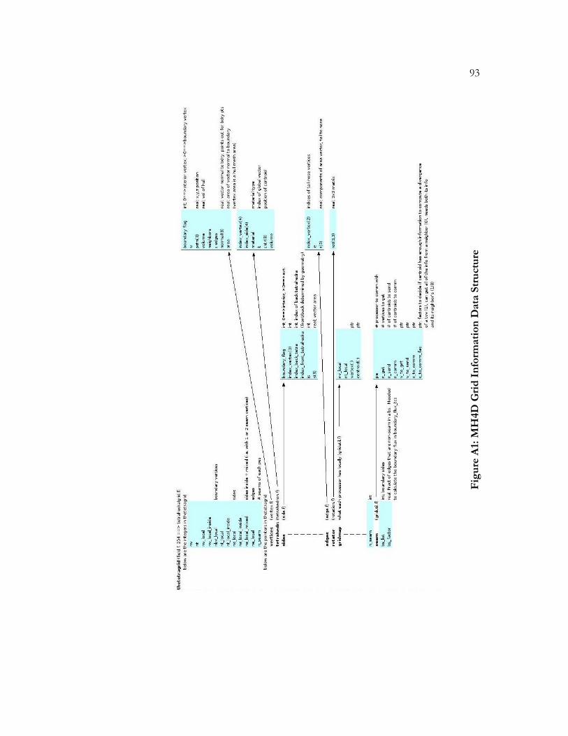
93
Fig
ure
A1:
MH
4D G
rid
In
form
atio
n D
ata
Stru
ctu
re
94
A.3 – MH4D Geometry Information and Proof that 0∇ • =B Inside the
Domain
This appendix section provides a proof that the divergence of magnetic field is
zero and briefly discusses some important computational characteristics of
MH4D. The appropriate geometric preliminaries are provided. This appendix
section is based on unpublished work by D. Schnack and R. Lionello.
In the MHD model, the vector potential, A, the magnetic field, B, and the current
density, j, are related by the curl operator,
= ∇×B A , (A1)
= ∇×j B , (A2)
and so
= ∇×∇×j A . (A3)
As required by Eqns. (A1) and (A2), 0∇ • =B and 0∇ • =j . The second order
differential operator in Eqn. (A3) is self-adjoint. Ideally, a computational MHD
code should preserve these solenoidal and self-adjoint properties.
Some geometric preliminaries are now given to provide a basis for the discussion
that follows. A tetrahedral cell of the primary mesh is shown in Figure A2.
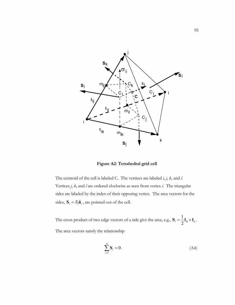
95
Figure A2: Tetrahedral grid cell
The centroid of the cell is labeled C. The vertices are labeled i, j, k, and l.
Vertices j, k, and l are ordered clockwise as seen from vertex i. The triangular
sides are labeled by the index of their opposing vertex. The area vectors for the
sides, ˆi i iS=S n , are pointed out of the cell.
The cross product of two edge vectors of a side give the area, e.g., 12i ik ij= ×S l l .
The area vectors satisfy the relationship
4
10i
i==∑S . (A4)
S j
l ij
l ik
l il
i
j
k
l C
C i
C j
Ck
C l
S i
Sk
S l mij
mik
mil
si
σij
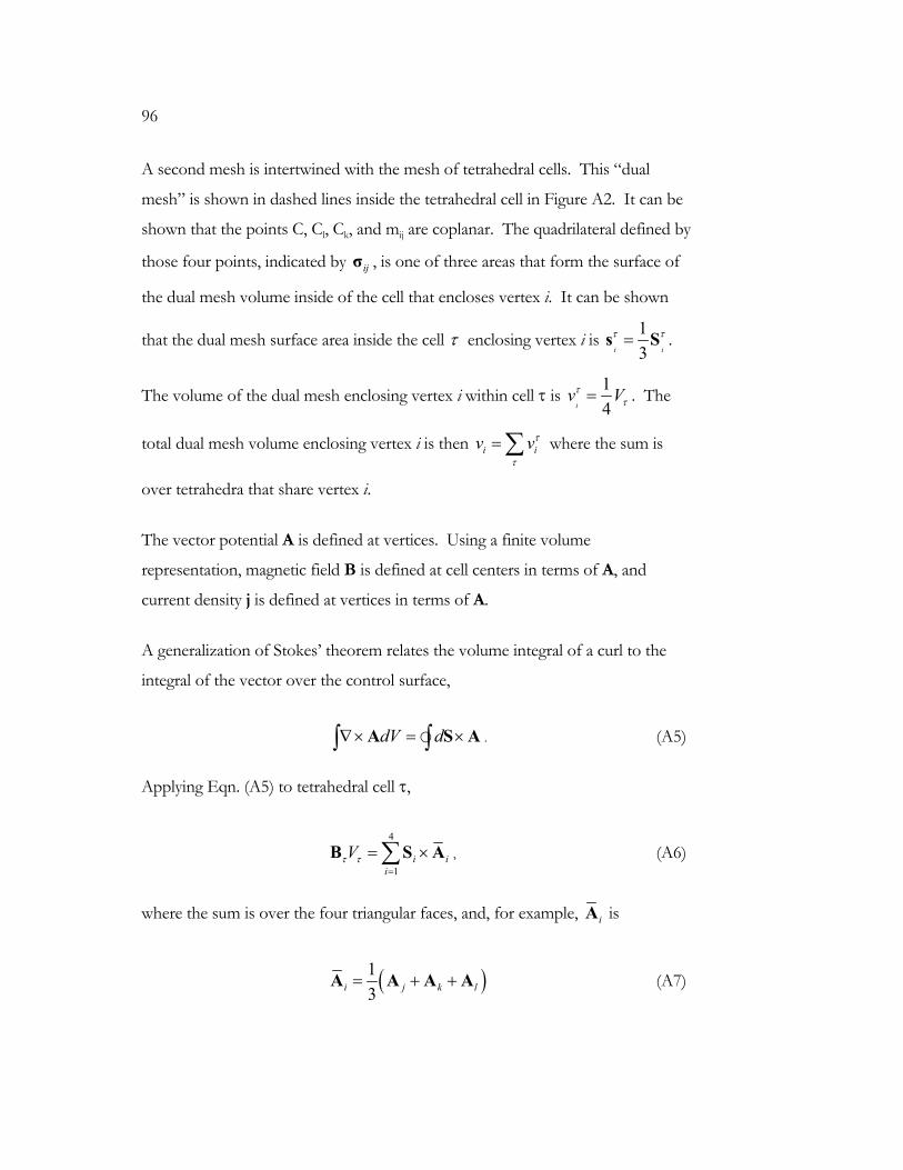
96
A second mesh is intertwined with the mesh of tetrahedral cells. This “dual
mesh” is shown in dashed lines inside the tetrahedral cell in Figure A2. It can be
shown that the points C, Cl, Ck, and mij are coplanar. The quadrilateral defined by
those four points, indicated by ijσ , is one of three areas that form the surface of
the dual mesh volume inside of the cell that encloses vertex i. It can be shown
that the dual mesh surface area inside the cell τ enclosing vertex i is 13i i
τ τ=s S .
The volume of the dual mesh enclosing vertex i within cell τ is 14i
v Vττ= . The
total dual mesh volume enclosing vertex i is then i iv vτ
τ
= ∑ where the sum is
over tetrahedra that share vertex i.
The vector potential A is defined at vertices. Using a finite volume
representation, magnetic field B is defined at cell centers in terms of A, and
current density j is defined at vertices in terms of A.
A generalization of Stokes’ theorem relates the volume integral of a curl to the
integral of the vector over the control surface,
dV d∇× = ×∫ ∫A S A . (A5)
Applying Eqn. (A5) to tetrahedral cell τ,
4
1i i
iVτ τ
=
= ×∑B S A , (A6)
where the sum is over the four triangular faces, and, for example, iA is
( )13i j k l= + +A A A A (A7)
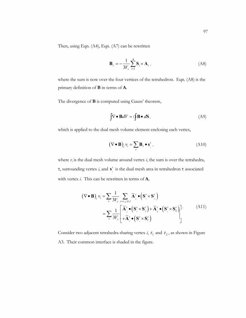
97
Then, using Eqn. (A4), Eqn. (A7) can be rewritten
4
1
13 i i
iVττ =
= − ×∑B S A , (A8)
where the sum is now over the four vertices of the tetrahedron. Eqn. (A8) is the
primary definition of B in terms of A.
The divergence of B is computed using Gauss’ theorem,
dV d∇ • = •∫ ∫B B S , (A9)
which is applied to the dual mesh volume element enclosing each vertex,
( )iii
v ττ
τ
∇ • = •∑B B s , (A10)
where vi is the dual mesh volume around vertex i, the sum is over the tetrahedra,
τ, surrounding vertex i, and i
τs is the dual mesh area in tetrahedron τ associated
with vertex i. This can be rewritten in terms of A,
( ) ( )( ) ( )
( )
, , ,
13
1 3
i
j i k i
l i
iii j k l
j k
l
vV
V
γ γ
τ τ τ
τ γτ
τ τ τ τ τ τ
τ τ ττ τ
=
∇ • = • ×
• × + • × = + • ×
∑ ∑
∑
B A S S
A S S A S S
A S S
. (A11)
Consider two adjacent tetrahedra sharing vertex i, 1τ and 2τ , as shown in Figure
A3. Their common interface is shaded in the figure.
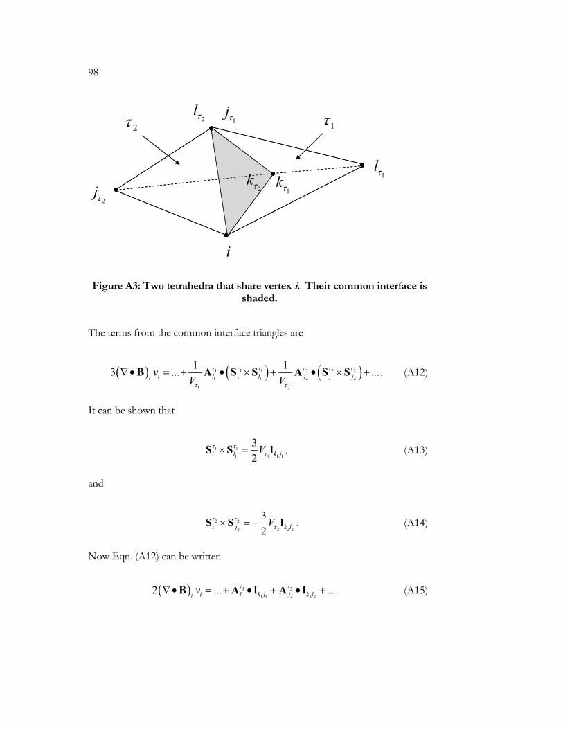
98
2jτ
2lτ
1lτ
1kτ
1jτ
i
2τ 1τ
2kτ
Figure A3: Two tetrahedra that share vertex i. Their common interface is shaded.
The terms from the common interface triangles are
( ) ( ) ( )1 1 1 2 2 2
1 1 2 2
1 2
1 13 ... ...i ii l l j ji
vV V
τ τ τ τ τ τ
τ τ
∇ • = + • × + • × +B A S S A S S , (A12)
It can be shown that
1 1
1 1 1 1
32i l k jVτ τ
τ× =S S l , (A13)
and
2 2
2 2 2 2
32i j k lVτ τ
τ× = −S S l . (A14)
Now Eqn. (A12) can be written
( ) 1 2
1 1 1 2 2 22 ... ...i l k j j k li
v τ τ∇ • = + • + • +B A l A l . (A15)
99
By construction, 1 2
1 2l jτ τ=A A and
1 1 2 2k j k l=l l , so the contributions from the
common faces cancel and ( ) 0i
∇ • =B . That is, the divergence of B vanishes at
interior vertices. In simulations, it has been found that 0∇ • =B is not enforced
at boundary vertices in the current implementation.
Using the same Stokes’ theorem approach, but now applied to the dual mesh
volume around a vertex, the current density j is defined
13i iv τ τ
τ
= ×∑j S B . (A16)
By inserting the expression for B given in Eqn. (A8), it can be shown that Eqn.
(A16) becomes
( )4
1
1 19i i j i i j j
j
vV
τ τ τ τ τ
τ τ =
= − − • • ∑ ∑j S S S S I A (A17)
This can be written as
( )( ) ( )
, ' jv τ τν ν
τ ν ν τ
ν ν= •∑∑j AM , (A18)
where ν indicates a vertex, ( )τ ν indicates a tetrahedron that shares vertex ν ,
and ( )ν τ is a vertex of tetrahedron ( )τ ν . This operator, τM is symmetric and
self-adjoint.
The more complicated geometry involved in Eqn. (A17) has prevented
theoretical analysis of ∇ • j (a quantity stored at cell centers). However
simulations show that 0∇ • =j is not enforced in the current implementation.

100
In summary, the MH4D formulation ensures 0∇ • =B for interior vertices.
Furthermore, the double curl operator is self-adjoint. However, 0∇ • =B is not
enforced at boundaries, and 0∇ • =j is not enforced.
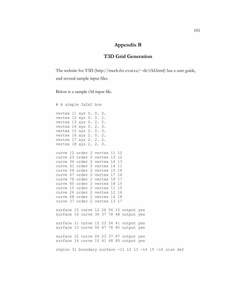
101
Appendix B
T3D Grid Generation
The website for T3D (http://mech.fsv.cvut.cz/~dr/t3d.html) has a user guide,
and several sample input files.
Below is a sample t3d input file.
# A simple 2x2x2 box vertex 11 xyz 0. 0. 0. vertex 12 xyz 0. 0. 2. vertex 13 xyz 0. 2. 2. vertex 14 xyz 0. 2. 0. vertex 15 xyz 2. 0. 0. vertex 16 xyz 2. 0. 2. vertex 17 xyz 2. 2. 2. vertex 18 xyz 2. 2. 0. curve 12 order 2 vertex 11 12 curve 23 order 2 vertex 13 12 curve 34 order 2 vertex 14 13 curve 41 order 2 vertex 14 11 curve 56 order 2 vertex 15 16 curve 67 order 2 vertex 17 16 curve 78 order 2 vertex 18 17 curve 85 order 2 vertex 18 15 curve 15 order 2 vertex 11 15 curve 26 order 2 vertex 12 16 curve 48 order 2 vertex 14 18 curve 37 order 2 vertex 13 17 surface 15 curve 12 26 56 15 output yes surface 16 curve 34 37 78 48 output yes surface 11 curve 12 23 34 41 output yes surface 13 curve 56 67 78 85 output yes surface 12 curve 26 23 37 67 output yes surface 14 curve 15 41 48 85 output yes region 31 boundary surface -11 12 13 -14 15 -16 size def
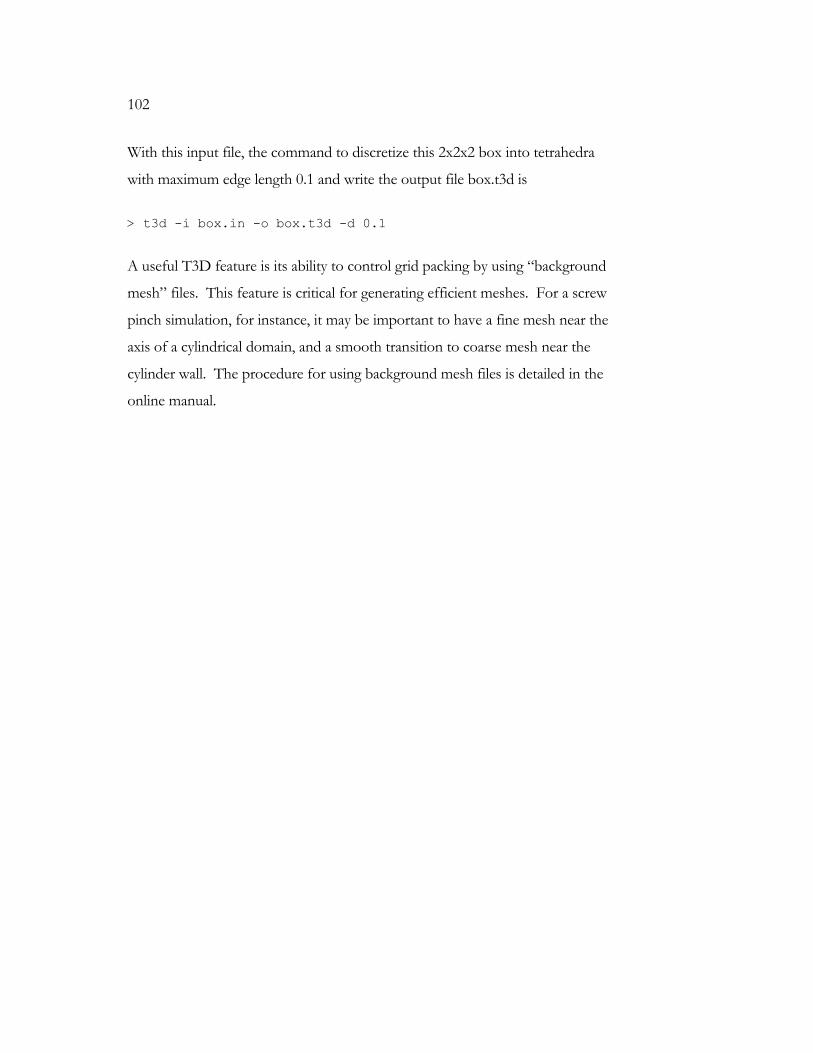
102
With this input file, the command to discretize this 2x2x2 box into tetrahedra
with maximum edge length 0.1 and write the output file box.t3d is
> t3d -i box.in -o box.t3d -d 0.1
A useful T3D feature is its ability to control grid packing by using “background
mesh” files. This feature is critical for generating efficient meshes. For a screw
pinch simulation, for instance, it may be important to have a fine mesh near the
axis of a cylindrical domain, and a smooth transition to coarse mesh near the
cylinder wall. The procedure for using background mesh files is detailed in the
online manual.