Fracture Mechanics of Concrete Structures, Proceedings FRAMCOS-2, edited by Folker H. Wittmann, AEDIFICA TIO Publishers, D-79104 Frei burg (1995)

DETERMINATION OF TENSION SOFTENING DIAGRAMS VARIOUS KINDS OF CONCRETE BY MEANS OF NUMERICAL ANALYSIS

Uchida, N. Kurihara, K. Rokugo and W. Koyanagi, Department of Civil Engineering, Gifu University, Gifu, Japan

Abstract Poly-linear approximation method combined with FE-analysis usmg fictitious crack model is introduced. accuracy and validity of the method are examined by the numerical analysis. The poly-linear approximation method is applied to various kinds of concrete including porous concrete and fiber reinforced high strength concrete to determine the tension softening diagrams and also to certify the validity of the method.

1 Introduction

It was about twenty years ago that Hillerborg et al. (197 6) proposed the Fictitious Crack Model (FCM). It is felt that the FCM is categorized into the old-fashioned model of concrete crack nowadays. However, the FCM has a sufficient ability to simulate the load-displacement response of concrete members with the development of mode-I crack in spite of its simplicity. The most essential material property for the analysis using the FCM is the tension softening diagram, which is the relation between decreasing transfer stress and the increasing crack opening in the fracture

17

process zone.

2

is approximated by of softening

fictitious crack determination of i +

or be

knee have been already ..... .., .. ""J'"'.Jlll ........... .....

softening a( w) from i Next, the load, the displacement

'-'0.J"''Jl"" ............ '""''"'I-'"""'""""" ...... ,.,_ ..... (COD) are calculated when i + node in the analytical model 1 (b) ),

''"'L._ ...... ,., ..... to agree the analytical load-displacement curve 1 ( c)). Then, the crack width at i + knee

analytical CODi+I when a(w) is determined l(d)),

18

0 p 0

2

0i+1

'--~~~~~_._~-F.:O~w

0 w i + 1 <E:---------

(a) Assumption of softening diagram (b) Model for analysis

p COD

i + 1

0 Oi+1 Oi +1

(c) Fitting of P - 6 ( d) Determination of crack

Fig. 1. Poly-linear approximation method

and finally, the stress at i +Ith knee point is as al CODi+iJ (Fig. l(a)).

The calculation program of the poly-linear approximation method is very simple, because it is only necessary to add the iteration routine to the crack extension analysis program using the FCM. Since variable for fitting is only the slope of a{ w), the iteration routine is also very simple. Furthermore, only stable load-displacement curves are needed to measured in the experiment, and it does not matter what type of specimen is used. However, it is still problem to determine the tensile strength (start

19

~~A .. -AAAAA,..., diagram). The determination of the tensile strength is in the following section.

tensile strength determination of tensile strength is also difficult in I-integral-based

tensile strength is used as the tensile strength in the .......... u· ........ A. ... ...., ..... I-integral-based method. The tensile strength is determined from

load the original poly-linear approximation method by ~~u_, ............... i~ ...... It is certain that the maximum load of the specimen depends on

.,....,_ .... _,_,_ ..... ..., strength of the concrete, but in the case of the other kind of concrete as fiber reinforced concrete the maximum load depends on the

A A~-AA,,_ property of the fiber rather than the tensile strength of the matrix concrete.

this reason, we assume the initial part of the softening diagram to be ...,...,_uc·•·"·"' ... plastic as shown in Fig. I (a). The tensile strength is determined to

perfect plastic stress when the fictitious crack length becomes the a given allowable difference between the experimental load-

, .... ,.,,_,. ....... _,....,.,T relation and the analytical one. The allowable difference (A.D.)

(1)

6 a is the displacement obtained through the analysis. PA l 6 a) and ) are the analytical and experimental loads corresponding to 6 a.

Young's modulus used in the this analysis is determined from the slope of load-displacement curve. The crack width of the end point

perfect plasticity part is determined to be the crack opening ...,.. ... ....,..., ............. ..., ......... ....,i ....... when the fictitious crack length becomes the longest. The

points beyond the perfect plasticity part are determined by the method ...... ...., ...... ..., .. , ... .., .......... in previous section.

method for the determination of tensile strength was examined numerical simulation. Fig.2 shows the fmite element mesh of side of the beam specimen, which is l 0 x l 0 x 40 cm and loaded

at third (loading span 30 cm). The 1/4 bilinear model (Rokugo et 989b)) shown Fig.3 was used for the FE-analysis of the load-load

displacement curve of the specimen and then the tensile strength and softening diagram were detennined. Fig.4 shows the relation between the perfect plastic tensile stress (tensile strength) and the fictitious crack length.

tensile stress when the fictitious crack length becomes the longest depends on allowable difference between the load-displacement curves,

20

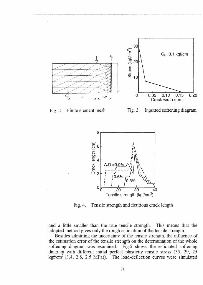
Fig. 2. Finite element mesh

30 C\J

E g ~20 CJ) CJ)

~ U5 10

1 kgf/cm

0 0.05 0.10 0.15 0.20 Crack width (mm)

Fig. 3. Inputted softening diagram

Fig. 4. Tensile strength and fictitious crack length

and a little smaller than the true tensile strength. This means the adopted method gives only the rough estimation of the tensile strength.

Besides admitting the uncertainty of the tensile strength, the influence of the estimation error of the tensile strength on the determination of the whole softening diagram was examined. Fig.5 shows the estimated softening diagram with different initial perfect plasticity tensile stress (35, 29, 25 kgf/cm2 (3.4, 2.8, 2.5 MPa)). The load-deflection curves were simulated

21

-Inputted o ft=35 kgf /cm2

0 29 6 25

0 0.05 0.10 0.15 0.20 Crack width (mm)

Fig. 5. Determined softening diagrams with different tensile strength

~ _g

1.5..------------.

0.5

-Inputted o ft=35 kgf/cm2

0 29 6 25

0.0 0.05 0.10 0.15 0.20 Displacement (mm)

Fig. 6. Simulated P - tJ

through the FE-analysis using the detennined softening diagrams and were shown in Fig.6. It is seen from Fig.5 that the estimated softening diagrams agree well with the true softening diagram, though the very initial part of the diagram depends on the tensile strength. All of the simulated load­deflection curves also agree well with the inputted load-deflection curve as shown in Fig.6. Consequently, it is not so important to determine the precise tensile strength for the determination of softening diagram by the poly-linear approximation method.

22

4...-~~~~~~~~--

- Inputted

0

o Determined

0.25 0.50 0. 75 1.00 Displacement (mm)

(a) P - o

10

0

............... Inputted

o Determined

0.25 0.50 0. 75 1.00 Crack width (mm)

(b) Softenig diagram

7. Detennined softening diagram of model FRC

Fig.7 shows the detennined softening diagram assuming the fiber reinforced concrete. The poly-linear approximation method is effective for the another kind of concrete like the fiber reinforced concrete of which softening diagram has a quite different shape.

It is noted that we could not obtain the softening diagram if we had used the tensile strength which was extremely different from the true tensile strength. In this case the solution would diverge or oscillate. In our experience, the smoother softening diagram would be obtained we used l wi + wi+I) /2 instead of wi for the crack with of i +1th knee point described in section 2.1.

3 Tension softening diagram of various kinds of concrete

3.1 Plain concrete The tension softening diagrams were detennined through the modified J­integral based method and the poly-linear approximation method for the nonnal stren!:,Tth concrete, high strength concrete and light weight concrete. The loading tests were perfonned according to the RILEM testing method. The water cement ratio of the nonnal strength concrete, the high strength concrete and the light weight concrete were 0.53, 0.27 and 0.46, respectively. The maximum aggregate size was 15 mm. The weight of unit volume was 1.63 t/m3 for the light weight concrete. The compressive strength of the normal strength concrete, the high strength concrete and the light weight

23

concrete were 407, 848 and 344 kgf/cm2 (39.9, 83.1 and 33.7 MPa), respectively. The size of beam specimen was 10 x 10 x 84 cm and loading span was 80 cm.

shows the load-deflection (loading point displacement) curves measured experiment. Fig.9 shows the softening diagrams determined

the modified I-integral-based method and the poly-linear approximation method. The softening diagrams detennined through two methods are similar to each other. The load-deflection curves were simulated through the FE-analysis using the determined softening diagrams and are shown in Fig. 8. The simulated load-deflection curves using determined softening diagrams through the poly-linear approximation method completely agree with the measured ones, whereas the load­deflection curves obtained from the modified I-integral-based slightly differ from the measured ones.

shapes of the tension softening diagrams of these concrete are ui;c.u, ..... ..,. ...

to each other and might be modeled by bilinear function. Consequently, data fitting technique assuming the bilinear function might be applied to these concrete.

3.2 No-fines porous concrete Since the crack opening displacement does not have to be measured applying the poly-linear approximation method, the notch does not have to be made. The poly-linear approximation method was applied to the no­fines porous concrete beam specimen without a notch. The mix proportions were W:C:G = 47:289:I624 and the average compressive strength was 188 kgf/cm2 (18.4 MPa). Three sizes of beam specimens were used. All the specimens had rectangular cross section with same width (10 cm). The heights of the cross sections were 10, 20 and 30 cm. These specimens are denoted as Pl 0, P20 and P30, hereafter. The lengths of the specimen were

the height. loading span lengths flexural test were height. The third point loading test was carried out. Only

load-deflection (loading point displacement) curve was measured. Fig. I 0 shows the load-deflection curves measured in experiment

Fig. I I shows the softening diagrams detennined through the poly-linear approximation method. The clear difference of the softening diagram among the three sizes of specimens was not observed, whereas the longer tail of softening curve was determined from the larger specimens. load-deflection curves were simulated through the FE-analysis using determined softening diagrams and are shown Fig. I 0. The simulated load-deflection curves using the softening diagrams of the different specimens are also shown in Fig. I 0. The simulated load-deflection curves using the softening diagram of the same specimen completely agree with the measured ones. In case of P20 and P30, there is a little difference of the

24

120---~~~~~-=~~--. - Exp.

30

0

o Poly-app.

------ J-int.

0.25 0.50 0. 75 1.00 Displacement (mm)

(a) N annal strength concrete

150 ............ Exp.

120 o Poly-app.

0

------ J-int.

0.25 0.50 0. 75 Displacement (mm)

(b) High strength concrete

1.00

ao....-~~~~~-==--~___, -Exp.

o Poly-app.

------ J-int.

0 0.1 0.2 0.3 0.4 0.5 Displacement (mm)

(c) Light weight concrete 8. P - bof plain concrete

25

-- Poly-app. -----·- J-int.

10

0 0.05 0.10 0.15 0.20 0.25 Crack width (mm)

(a) N annal strength concrete so.--~~~~~--~~--,

-- Poly-app. ------- J-int.

0 0.05 0.10 0.15 0.20 0.25 Crack width (mm)

(b) High strength concrete 25r----~~~~~~~~--,

--- Poly-app. ------- J-int

5

0 0.05 0.10 0.15 Crack width (mm)

(c) Light weight concrete Fig. 9. Softening diagram

concrete

c c 0 ~

Fig.

1.5--------E-x-p.--...........,

o Ana. use P1 O

0.05 0 5 0.20 Displacement (mm)

(a) 5.0---------E-x-p-. -

4.0

0.0

10.0

7.5

0 0 P20

6 P30

0.05 0.10 0.15 0.20 Displacement (mm)

(b) P20

-Exp. 0 P10

P20 P30

0.05 0.10 0.15 0.20 Displacement (mm)

(c) P30 P - bof no-fines porous concrete

26

0 0.2 0.4 0.6 0.8 Crack width (mm)

(a) PlO

0 0.2 0.4 0.6 0.8 Crack width (mm)

(b) P20 20

0 0.2 0.4 0.6 0.8 Crack width (mm)

(c) P30 Fig. 11 Softening diagram of no­

fines porous concrete

Table 1. Mix proportions and strengths of FRC

Unit weight {kg/m3} Strength {kgf/ cm2

}

Concrete w c s G F com. flex.

AF 189 674 1348 - 28 859 134

VF 203 726 1276 - 28 827 109

SF 140 500 889 774 156 945 137

maximum load between the load-deflection curve usmg the softening diagram of PIO and the measured one.

3.3 Fiber reinforced high strength concrete The tension softening diagrams were determined through the poly-linear approximation method for three kinds of fiber reinforced high strength concrete. Aramid fiber ( tj>0.4 x 30 mm, strength: 3.0x104 kfg/cm2 (2.9 GPa)) , vinylon fiber ( cp0.38 x 30 mm, strength: 1.1x104 kfg/cm2 .1 GPa)) and indented steel fiber ( cpO. 6 x 30 mm, strength: 1. 2 x 104 kfg/cm2 (1.2 GPa)) were used. These fiber reinforced concrete are denoted as AF, VF and SF, hereafter. Volume content of the fiber was 2.0 %. mix proportion and strength properties are shown in Table 1. The size of beam specimen without a notch was 10 x 20 x 70 (widthxheightxlength) cm and the loading span was 60 cm. The third point loading test was carried out, and the load-deflection (loading point displacement) curve was measured.

Fig.12 shows the load-deflection curves and Fig.13 shows the softening diagrams determined through the poly-linear approximation method. It is seen from these figures that the poly-linear approximation method is also effective for the fiber reinforced concrete. It is noted that the fracture energy of the aramid fiber reinforced concrete was about twice as large as that of the steel fiber concrete.

The shape of these fiber reinforced concrete might be modeled by trilinear function, that is, the initial softening part, the plastic part and softening part, as shown in Fig.14. These three parts would depend on the characteristics of the matrix concrete, bridging of fiber and pull-out or cut-off of the fiber, respectively.

4 Conclusions

Although it is difficult to determine the tensile strength precisely, poly­linear approximation method is very effective for the determination of

27

15

10

5

0

15

0

............... Exp.

0 Poly-app.

2.0 4.0 6.0 8.0 Displacement

0

0.5 1.0 1 .5 2.0 Displacement

(b) VF

0

0 1.0 Displacement

(c) SF

12 P-bofFRC

28

60

~ 45 u ~ O'>

:s:. ;- 30

Cl') CD :a... ......

U)

15

0

60

~ 45 J2. -O> :s:. '-'30

0

3

2.0 4.0 6.0 8.0 Crack width (mm)

(a) AF

1.0 2.0 3.0 4.0 width (mm) VF

0 Crack

analysis is necessary method, but it is very easy to make

extension analysis experiment .,,,.,,,,..,..,,.,..,,,..., for

5

authors ~~·T•~r-YYH Foundation's Research

6

Hillerborg, A., Modeer, M. formation crack and finite elements. ,.__,..., ... ,..,. ...... X.Z. and hardened cement paste mortar. (eds S.P. Shar, S.E. Swartz London, 307-316.

Kitsutaka, Kamimura, analysis

29

453, 15-25 .(in

Ward, R.J. (1989) A novel testing technique for post-peak · cementitious materials. Toughness and

Mishasi, Wittmann),

of concrete

981) growth and development of fracture zone in concrete and

Jl.J'->.L•~-.._.__._h Mat., Lund materials. TVBM-1006, Div. of

Recommendation (1983) the fracture and concrete means of tests on notched

Materials Structures, 18, 285-290. P.E. and P.H. (1986) to strain

softening failure concrete, in Fracture Toughness Fracture

Rokugo, K.,

Concrete ( ed F .H. Wittmann), Elsevier Science Publishers, 163-175.

Seko, S. and Koyanagi, W. 989a) Tension fiber reinforced concrete, in Fracture of

S.P. Shar, S.E. Swartz and B. Barr), Elsevier 513-522.

T. and Koyanagi, W. (1989b) Testing _.__.__,_...,,a_,_v,..1-0 to determine strain · curves and fracture energy

in Fracture Toughness Fracture Energy (eds Tkahashi Wittmann), Rotterdam, 153-

Koyanagi, W. 1) A./"'"""' ...... _ ... .__.L.__._,...,..__,_'U,_._ ...

by means of bending tests. 426, 203-212.(in Japanese) I Concrete

84.

30