1

XXXV CONFERENZA ITALIANA DI SCIENZE REGIONALI

DETERMINANTS OF INTERNATIONAL TOURIST CHOICES IN ITALIAN PROVINCES: A JOINT DEMAND-SUPPLY APPROACH WITH SPATIAL EFFECTS

Eleonora LORENZINI1, Maurizio PISATI2, Tomaso POMPILI3

ABSTRACT

This paper uses a unilateral gravity model augmented by including spatial effects to investigate

the determinants of international tourist choices (arrivals, overnight stays, length of stay,

expenditures), in Italian provinces (NUTS 3). The elements of originality are that both demand

and supply variables are considered in the model and possible spillover effects originating from

contiguous provinces are analysed using a spatial Durbin model. Moreover, the distance between

origin and destination is included to take into account travel costs. Results indicate the

importance of both demand and supply factors and demonstrate the existence of a competition

effect generated by the tourism capacity of contiguous provinces.

Keywords: tourism, spatial spillover, gravity model, regional economic activity

JEL: C31, L83, R12

1 Dipartimento di Scienze Economiche e Aziendali, Università di Pavia. 2 Dipartimento di Sociologia e Ricerca Sociale, Università di Milano-Bicocca. 3 Dipartimento di Sociologia e Ricerca Sociale, Università di Milano-Bicocca. Corresponding author: tomaso.pompili@unimib.it

2

1. INTRODUCTION

According to a recent UNWTO World Tourism Barometer, receipts in destinations worldwide

from expenditure by international visitors on accommodation, food and drink, entertainment,

shopping and other services and goods, reached an estimated US$ 1159 billion in 2013. Growth

exceeded the long-term trend, reaching 5% in real terms. The growth rate in receipts matched the

increase in international tourist arrivals, also up by 5%, reaching 1087 million in 2013.

International tourism (travel and passenger transport) accounts for 29% of the world’s exports of

services and 6% of overall exports of goods and services. As a worldwide export category,

tourism ranks fifth after fuels, chemicals, food and automotive products, while ranking first in

many developing countries. These figures demonstrate the importance of the tourism sector in

the world economy.

Since the tourism market increasingly operates as a competitive one, where destinations at

different territorial levels are horizontally differentiated (Marrocu and Paci, 2013), understanding

the determinants of competitiveness is crucial to address tourism planning and destination

management. Research trying to explain tourism flows and expenditures for different

destinations has so far adopted either a tourism-demand or a tourism-supply approach. Whereas

on the one hand the former ignores the product specificities (Papatheodorou, 2001), the latter,

on the other, fails to take into account the characteristics of the tourist origin markets. In recent

years attempts to merge the two views have come from scholars using origin-destination models

(O-D), which have been able to consider both effects simultaneously. The majority of these

studies investigates the determinants of tourist flows at the local level, i.e. at the regional or

provincial level. Indeed, while tourism competitiveness is prevalently studied at the country level,

the local level - the territory - more than the macro and the micro level, determines the capacity

of a country to be competitive (Courlet, 2008) also in tourism (Lorenzini et al., 2011). When

using a territorial perspective, recent research highlights also the importance of considering

spatial dependence and hence local spillovers in estimating the impact of different variables in

tourism attractiveness.

This paper contributes to this literature by investigating the determinants of tourist flows to 103

Italian provinces (NUTS 3) from the top 20 origin countries. The elements of originality with

respect to previous literature are the following. First, we estimate a (unilateral) gravity model

considering demand- and supply-side factors jointly. The observations of our cross-section

database reflect the foreign tourist arrivals, expenditures, length of stay and overnight stays in

103 Italian province from the 20 highest spending countries of origin. We will disentangle the

effects of both demand and supply variables on a province’s tourism flows and exports. Among

the former ones, per capita GDP levels, population and a measure of relative price will be

considered. Among the latter ones: per capita GDP levels at destination and supply variables such

as capacity constraints of tourist accommodations; tourism and transport infrastructures; crime,

cultural and environmental capital. Moreover, the role of the distance between origin and

destination is taken into account as a proxy for travel costs.

Second, our model includes spatial effects to examine the possible spillovers originating from

supply variables in contiguous provinces. Besides the Spatial Autoregressive model usually

3

employed in tourism studies, following the suggestion of Halleck Vega and Elhorst (2013), spatial

effects will be analysed using the spatial lag of independent variables as well. Finally, we consider

as dependent variables foreign tourist arrivals, tourist expenditures, length of stay and overnight

stays. The variable tourist expenditures, recently made available by the Bank of Italy, is very

informative because it captures not only the number of tourist arrivals and stays, but also their

contribution to a destination’s GDP. However, given that sample selection bias due to the

survey origin of the data may affect the goodness of the results, we compare the results of this

model with those for overnight stays.

Italy has been selected as a case study for various reasons. First, it is one of the world top

countries for tourism arrivals and overnight stays. In 2012 it was fifth for number of

international arrivals (46 million according to World Bank Database) after France, USA, China

and Spain. Second, in Italy tourism accounts for 10.3% of GDP and 11.6% of employment.4

Moreover, the high diversification of its provinces in terms of natural, cultural, environmental

and business endowments makes of Italy a good case to study the different impact of supply

variables. We believe that the province can be a proper unit of analysis since its size is enough

large to capture agglomeration economies while at the same time enough small to highlight the

differences between territories.

Italian provinces have been the focus also of the analyses carried out by Massidda and Etzo (2012)

and Marrocu and Paci (2013). While they examined the determinants of domestic tourism flows,

we are interested in foreign flows. Indeed, these latter are a relevant and increasing share of the

total, accounting for 47.4% in 2012 compared to 43.3% in 2008. Moreover they increase at a

higher rate with respect to domestic tourism. In the period 2008-2012 inbound tourist arrivals

and nights have grown by 3.1% and 2.2% respectively, compared to 0.5% and -1.1% of domestic

ones. This because foreign flows, like exports, are exogenously determined and independent

from domestic economic conditions and business cycle. For this reason they can foster tourism

demand also in periods of internal stagnation.

The paper proceeds as follows. Section 2 provides an examination of the relevant literature about

how to model tourist flows’ determinants. Section 3 describes the data and the variables

employed in the analysis. Section 4 illustrates the methodology adopted. Section 5 shows the

main results and section 6 concludes with policy suggestions.

2. LITERATURE REVIEW: MODELLING TOURISM FLOWS

Research trying to explain tourism flows to destinations has prevalently adopted either a

tourism-demand or a tourism-supply approach.

Tourism demand studies assess the importance of country-of-origin factors in determining the

incoming of inbound tourist flows. The majority of the econometric studies examine the

demand of tourism for one or more destination countries originating from a set of top partner

countries using time series or panel data analysis. Income is the most important explanatory

4 WTTC - Travel & Tourism Economic Impact 2014 Italy, as reported by Enit.

4

variable: Crouch (1994) reveals that the income elasticity generally exceeds unity but is below

two, which implies that international travel is still regarded as luxury consumption. Economic

theory also indicates that the price of tourism products and services is related negatively to

tourism demand. Additional variables sometimes incorporated in the models are marketing

expenditure, consumer tastes, consumer expectations, habit persistence, population of the

country of origin and one-off events (Song and Witt, 2000). One of the advantages of demand

models is that they are employable as a short-run forecasting tool to estimate the demand for a

destination country from its main markets.

Tourism-supply studies, instead, aim at estimating the importance of destination supply factors

in influencing the arrival, stay and expenditure of international or domestic tourists. The

explanatory variables generally used are: population, income per capita, hotel capacity, price,

infrastructures, agglomeration economies, cultural and natural capital, crime, climate,

institutional capacity.

Both demand and supply models suffer from at least one drawback. On the one hand, the former

ignores the product specificities (Papatheodorou, 2001); on the other, the latter fails to take into

account the characteristics of the tourist origin markets.

In recent years few scholars have succeeded in merging the two views by using spatial interaction

models, i.e. gravity or origin-destination (O-D) models, to consider both effects simultaneously.

Marrocu and Paci (2013), Massidda and Etzo (2012), de la Mata and Llano-Verduras (2012), Keum

(2010), Deng and Athanasopoulos (2011), Patuelli et al. (2013), all employ spatial interaction

models considering bilateral tourism flows between regions of a same country to take into

account both demand and supply determinants. These models reveal to policy makers and

tourism stakeholders what elements of the supply help in attracting tourism flows and what are

the determinants of the arrivals on the demand side. Massidda and Etzo (2012), for instance, find

that the main determinants of domestic tourism demand in Italian provinces are relative prices

and per capita tourist income, jointly with environmental quality.

Although robust empirical evidence supports the use of gravity models not only for trade in

goods but also in services,5 until recently their application to trade in services and tourism was

threatened by the lack of a theoretical background. Morley et al. (2014) contribute to fill in this

gap in the literature by providing a theoretical foundation, derived from the consumer’s utility

theory, for the current version of the gravity equation applied to tourism.

Following the above mentioned empirical and theoretical literature, in this paper spatial

interaction models are used to examine the demand and supply determinants of tourism flows to

Italian provinces. A point of departure from the previous literature is that our interest is focused

on international tourism, while most of the previously cited empirical studies are interested in

modeling domestic tourism flows. In doing so they consider bilateral tourism flows between

regions of a same country, while we consider unilateral tourism flows from the top 20 origin

countries of provenance of tourism flows to Italian provinces.

5 Kimura and Lee (2006) show that trade in services is better predicted by gravity equations than trade in goods.

5

Even though spatial interaction models provide a good starting point for our analysis, recent

tourism literature has highlighted also the importance of considering the likely impact of spatial

spillover effects when dealing with the study of regional tourism determinants. Marrocu and Paci

(2013), for example, find significant impact of both demand and supply factors, but they warn

that if spatial spillover effects are not considered the usual omitted variable estimation problem

may arise making the gravity estimates upward biased.

Moreover, the authors highlight a further advantage of incorporating spatial dependence. Indeed,

understanding the distinction between the relative effect of internal and external determinants of

tourism flows may have important implications for policy makers and tourist operators.

Following this suggestion, our gravity model has been augmented by including variables able to

capture spatial spillover effects. Yang and Wong (2012) provide a framework for the

interpretation of spillovers, identifying the following typology:

• productivity spillovers: they may result, first, from labor movements across regions. Once

staff members move, knowledge and skills move as well, contributing to the tourism

growth of the host region. Second, from demonstration effects associated with knowledge

diffusion processes, whereby firms tend to learn from their counterparts in regions with

higher productivity, consciously or unconsciously. Third, from competition effects;

• market access spillovers: when one city or region possesses a high share of a certain market,

its neighboring cities are highly likely to receive the market access spillover and gain easy

access to this market;

• joint promotion: collaboration in marketing amplifies the overall and the single destination

attractiveness.

Since these effects are difficult to be captured by spatially lagged proxies, it is common practice

in the literature to use Spatial Autoregressive (SAR) Models. They consist in augmenting the

basic model with an additional spatial autoregressive term, based on a connectivity matrix for

destination dependence. Yang and Wong (2012), indeed use this method in their study on 341

cities in mainland China and confirm the presence of spatial autocorrelation. Similarly, Marrocu

and Paci (2013) find highly significant evidence of neighboring provinces spillovers, which

amplify the impact of internal determinants of tourism flows.

Despite its prevalent use in tourism studies, the SAR model is not able to disentangle the causes

of spatial spillovers, e.g. if and how differences in the carrying capacity or resource endowment

of one destination affect the differences in tourism flows’ attraction. In order to overcome this

limit, Halleck Vega and Elhorst (2013) suggest that spatial effects should be analysed using the

spatial lag of some independent variables as well. Only a few empirical works make use of this

estimation strategy in tourism studies. Among them, Yang and Fik (2014) use a Spatial Durbin

Model (SDM) including spatially lagged autoregressive and explanatory variables. In this way

they are able to provide insights on the cross-city competition/agglomeration effects. 6 In

particular, they note that a positive association between spatially lagged explanatory variables

and dependent variable indicates an agglomeration effect, while a negative association points at a

competition effect. Their analysis on tourism growth in Chinese prefectures indicates that more

6 Other scholars use the terms substitution and complementarity in order to define these effects.

6

tourism resource endowments in the neighbouring regions hinder local inbound tourism growth

because of the competition effect across nearby cities. Likewise, Patuelli et al. (2013), studying

the impact of World Heritage Sites endowment on 20 Italian regions’ flows using a spatial

interaction panel data model, find that WHS generate a phenomenon of spatial substitution.

Capone and Boix (2008), instead, study the Italian case but they use a supply-model and their

reference unit is the Local Labour System. At this scale, they do not find statistically significant

coefficients for spatial spillovers either using the lag of the independent variables, the

Autoregressive or the Spatial Error models.

In what follows the determinants of inbound tourism flows to Italian provinces are examined

using a spatial interaction model augmented to account for spatial dependence. Further details on

the methodology are provided in the next section.

3. DATA AND VARIABLES

Data used in the analysis refer to the Italian provinces of destination of tourism flows (n=103)

and the top 20 countries of origin (P=20).7 The number of observation is then equal to n x P =

2060. Figure 1 and 2 show the distribution of tourist flows in the 103 considered provinces.

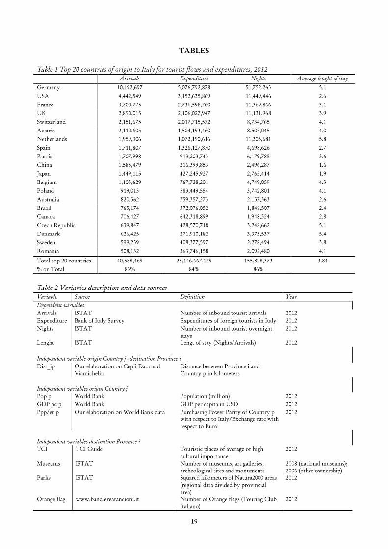
Table 1 shows the list of the top 20 origin countries and the arrivals, expenditures, nights and

average length of stay for each of them.

Table 2 shows the complete list of variables, the source of the data, the definition and the year of

reference. Most of the variables are collected for the year 2012, with the exception of some

independent variables for which a different year has been chosen. Table 3 shows the main

descriptive statistics and Table 4 the correlation matrix.

3.1 Dependent variables

Tourist arrivals and tourist expenditure (receipts) are the most commonly used tourism demand

measures in empirical studies (Song et al., 2010). Tourist arrivals are important for tourism

product/service suppliers in planning their supply capacity. For example, the decisions of

investing in new hotels and new aircrafts rely largely on accurate forecasts of tourist arrivals

(Sheldon, 1993). However, the tourist volume measure does not take account of the economic

impact of tourism on the related sectors/activities. Hence, tourist expenditure (that is, the

receipts of the destination) is the main concern of governments and central banks. Moreover,

when foreign tourist expenditures are used, they are a direct measure of tourism exports.

Although expenditures would be our main variable of interest, this variable suffers from biases

due to problems in the data collection process by means of surveys. Hence, following the

relevant literature we investigate the determinants of both arrivals and expenditures. Moreover,

7 In the last decades the number of Italian provinces has changed from 103 in 1992 to 107 in 2001 to 110 in 2004. We have chosen the former classification since some variables were not available for the latter ones. As for the number of origin countries included in the analysis, we have selected the top 20 which account for 83% of arrivals, 86% of nights and 84% of foreign tourists’ expenditure.

7

as a robustness check, our model will be also checked using overnight stays as independent

variable. Finally the model is tested also on the dependent variable average length of stay.

As anticipated, data on arrivals and nights are retrieved from the Italian Statistical Office

(ISTAT), while data on expenditures are retrieved by the Bank of Italy and collected by means of

a survey at the borders and at the main points of arrival of international tourists (airports,

railway stations).

3.2 Explanatory variables

Moving on to examine independent variables, for the sake of clarity we describe, first, the one

referring both to origin and destination, then those related only to the origin countries and,

finally, those related only to the destination provinces.

3.2.1 Origin-Destination variable (demand side)

The distance between origin and destination measured in kilometers is included in the model in

order to account for (both monetary and time) travel costs. This is a standard practice in tourism

studies as well as in gravity equations. Given the high number of origin-destination pairs, the

distance has been measured as follows. The distance between extra-European countries and

Italian provinces is obtained by adding up the distance between the capital of the country and

Rome (where the tourist is assumed to land) plus the distance between Rome and each capital of

province. The distance between European countries and Italian provinces is given by the distance

between the capital of the country and the capital of the region. When the distance between

capital of the region and capital of the province exceeds 100 km, a specific distance has been

measured. Distance is expected to have negative impact on tourist flows.

3.2.2 Origin variables (demand side)

Population of the country of origin measures the size of each specific market. It is expected to be

positively correlated with tourist flows.

As explained in Section 2, income in the origin country is one of the main determinants of

tourism flows in demand models. In our specification we use gross domestic product (GDP) per

capita in order to distinguish the effect of market size (population) from that of income.

The necessity to include variables that represent tourism prices imposes a big challenge to

empirical tourism research due to the difficulty of finding proxies for tourism prices. For our

purpose a price level index has been calculated in order to account for the differences in the

purchasing power parity (PPP) between origin countries. The index is obtained using the PPP

conversion factor for GDP but rescaled in order to consider Italy as the reference country. The

result has then been divided by the exchange rate of the country with respect to the Euro (the

Italian currency). The obtained price index varies for country of origin while it is constant for

destination units since a relative index of tourism prices is not available for the Italian provinces.

As shown in Table 4, the variable is highly correlated with GDP per capita (0.79). Consequently,

it has been excluded from the regression analysis.

3.2.3 Destination variables (supply side)

8

3.2.3.1 Leisure tourism attractions

Natural and cultural amenities are a relevant pull factor of the Italian touristic supply. Given the

diffusion of the cultural endowment on the national territory and the difficulty of finding a

single proxy for it, we have chosen more than one variable to disentangle the diversity of

possible effects.

The variable TCI measures the touristic places of average or high cultural importance, as

indicated by the Guide of the Touring Club Italiano (TCI), the top Italian association

operating in the fields of tourism, culture and the environment from over a century.

TCI also sponsors the program Orange Flags, established in 1998 in order to identify and

promote the smaller cities of the Italian inland that are enriched by a historic, cultural and

environmental heritage, and quality in the visitors’ welcoming. The number of Orange Flags of

the Province (Orange Flag) is included as a proxy of the quality of inland extra-urban tourism.

The number of museums (Museum) is an additional proxy for cultural endowment. It includes all

museums, art galleries, archeological sites and monuments of the province.

Coast is a proxy for the coastal surface of the province, intended to measure the importance of

sea-sun-sand attractions. The variable Blue Flag, instead, indicates the number of beaches awarded

of the quality label by Legambiente.

Park indicates the surface area of the province belonging to Natura 2000, a network including all

protected natural areas. Since this variable is only available at the regional level, the squared

kilometers of protected areas of a region have been divided according to the weight of the

province on the regional surface area.

Given the high collinearity of Parks with Mountain, indicating the number of squared kilometers

of mountain surface per province, the former variable has been used also as a proxy of the latter.

The variable Restaurant, indicating the number of restaurants awarded with at least one Michelin

star, was selected to assess the role played by gastronomy and culinary reputation in attracting

tourism flows. This variable has never resulted significant and its inclusion worsened the

goodness of fit of the models, hence it has been excluded from the analysis.

All variables referring to cultural and natural resources are expected to have positive coefficients.

Finally, following other studies (Eilat and Einav, 2004; Massidda and Etzo, 2012), we have

collected data for the diffusion of crime. The data collected from ISTAT refer to the number of

reported crimes but, in our opinion, do not adequately reflect the actual level of criminality in

the Italian provinces. This may be due to the level of legalistic culture and the confidence in the

judicial system which are not homogenously distributed in the national territory. Not

surprisingly, Crime has never resulted statistically significant in any model and hence has been

excluded from the analysis.

3.2.3.2 Business tourism attractions and quality of the services

GDP per capita (GDP pc i) is an indicator of the level of economic development at the

destination and can be interpreted in two ways (Marrocu and Paci, 2013). First, as an indicator of

business trips importance, since a high income area is more likely to attract business tourism.

Second, as an indicator of quality of the services, since a high income region provides better

quality public and territorial services (public transport, health care, law enforcement and so on).

9

In both cases it is expected to have positive influence on arrivals, while its expected sign is

ambiguous for overnight stays and length of stay since business trips are usually shorter than

leisure ones.

3.2.3.3 Tourism services capacity

The number of beds (Beds) is an indicator of the capacity of the tourism sector in a given

province. It can also be considered as a proxy of investment in tourism infrastructure.

Furthermore, a certain volume of accommodation is necessary for a destination to reach the so-

called ‘critical mass’ (Naudé and Saayman, 2005) needed to attract investments (i.e., convince

airlines to establish routes or justify investment in complementary infrastructures). Data for this

variable refer to the year 2009 because some time is needed in order for the effects to have place.

Besides, the number of employees in commerce and tourism-related services and its ratio with

respect to total employees have been considered as indicators of specialization in tourism.

However, given the high correlation with Beds, the two variables have been used as alternatives.

Beds has finally been selected because when the model has been estimated with both explanatory

variables only Beds resulted significant. Moreover, when considered as alternatives, the goodness

of fit of the model was higher when using Beds.

3.2.3.4 Accessibility

Many studies have investigated the tourist behavior towards the degree of congestion in the

destination (Massidda and Etzo, 2012; Saarinen, 2006; Marrocu and Paci, 2013). Population

density (Popden) is the variable usually used to verify the preference of tourists for more or less

crowded areas. In our model we have preferred to use as alternative variable the total surface area

of the province (Area size), which in our database is highly (negatively) correlated with Popden,

in order to verify this effect. Moreover, we have included a dummy variable for provinces with

population greater than one million inhabitants (Popbig) in order to verify the effect of

urbanization economies. This variable has been preferred to the number of residents in the

province in order to avoid collinearity problems with other variables.

It is also worth noting that total surface can be thought as a measure of accessibility as well, since

a larger area can imply a higher dispersion of attractions and a higher effort to reach them.

Additionally, to account for the level of accessibility, the number of airports with more than

10,000 passengers was considered (Airport). As an alternative variable, an index of accessibility

(Infrastructure) was tested. Results coincided and hence the number of airports has been preferred

because of the higher reliability of the variable.

In order to apply the gravity model as specified by Morley et al. (2014), all variables have been

transformed in natural logarithm with the exception of the dummy variable Popbig. As a

common practice in the literature, in order to avoid negative values, the natural logarithm

transformation has been applied to the value of the variable plus one, so as to obtain a value of

zero in the transformed variable in correspondence with a value of zero in the original one.

Since both dependent and independent variables are expressed in logarithms, estimated

coefficients can be interpreted as elasticities.

10

4. ECONOMETRIC STRATEGY

We use a regression model whose general specification is (Elhorst 2014):

0

1 1 1 1

n K L n

ip ij jp k ipk l ij jpl i ip

j k l j

y w y x w zβ ρ β ϑ γ ε= = = =

= + + + + +∑ ∑ ∑ ∑ (1)

where ipy denotes the value taken by response variable y on province i and origin country p; 0

β

denotes an overall constant; ijw denotes the spatial weight connecting province i with province j;

ρ denotes the endogenous interaction coefficient; ipkx denotes the value taken by regressor kX

on province i and origin country i; kβ denotes the regression coefficient associated with regressor

kX ; jplx denotes the value taken by regressor lZ on province i and origin country p;8 lϑ denotes

the exogenous interaction coefficient associated with regressor lZ ; iγ denotes the random effect

for province i; and ipε denotes the error term.

All model unknowns are estimated by maximum likelihood using the Stata user-written

command xsmle (Belotti et al. 2013).

Following Florax et al (2003) we estimate first a simple a-spatial model and introduce the

complexity successively. Hence, in the first specification we estimate a basic gravity model setting 0ρ = and 0lϑ = . Next the gravity model is augmented to take into account spatial

spillovers. The Spatial Durbin Model of Equation 1 is estimated including the spatial lag of the

dependent variable and of the regressors referring to the province of destination.

The spatial distance between provinces is represented by the symmetric n by n matrix W whose

entries are the geographical distances in kilometres between each province’s centroid with a cut-

off point of 100 kilometres. This threshold has been chosen because it is unlikely that tourists

travel daily a greater distance. In order to check the robustness of the results a different

specification of W with a cut-off point of 80 kilometres has been tested but results remained

unchanged. On the contrary, a lower cut-off point has not been used because some provinces

would have remained isolated.

5. RESULTS

Our estimation strategy involved testing international tourist expenditures as the main

dependent variables. However, since the variable suffers from biases due to problems in the data

collection process by means of a survey, we paired it with a more traditional dependent variable,

i.e. international tourist arrivals. First, for each of them we estimated a model with both demand

and supply determinants but without spatial effects; at a second stage we re-estimated a model

8 In our specification we are interested only on the spatial lag of destination variables in province i while we omit the spatial lags of variables related to origin country p since we believe that spillover effects among different origin countries are not relevant.

11

including also spatial spillover effects. Finally, as an extension and robustness check, the baseline

and the spatial models were estimated also for two other dependent variables, namely

international tourist overnight stays and international tourist average length of stay, both of

which are proxies of the tourist propensity to spend at destination.

5.1 The basic model

First of all we estimated the a-spatial specification of our model for expenditures and nights. The

estimated models are shown in Table 5 columns 1 and 3.

As for tourist expenditures, the a-spatial model explains 36% of total variation of international

tourist expenditures. Estimated coefficients are significant for nine out of fifteen independent

variables (of which seven at 1%). Actual signs correspond to expected signs for all nine significant

variables. All demand-side regressors are statistically significant with coefficients equal to 1.90 for

country-of-origin per capita GDP and 0.81 for population. Origin-destination distance has a

high coefficient equal to -1.85 while significant supply-side variables are, in descending order:

provincial per capita GDP (2.72), museums (1.42), Touring Club landmark cities (1.24), the

dummy for big city provinces (1.16), beds (1.07), top quality beds (0.63). This result implies that

provincial per capita GDP, which is a proxy of both business tourism attractiveness and quality

of territorial services, is the only supply-side element with greater impact than demand-side

elements. Cultural tourism attractiveness, carrying capacity and quality of the accommodation

have a sizeable impact as well, although relatively less important. International tourist

expenditures seem therefore to be mostly influenced by high spenders such as business and

cultural tourists, as well as by the country of origin of the flows.

As for international tourist arrivals the a-spatial model explains 71% of total variation. Estimated

coefficients are significant for ten out of fifteen independent variables (of which six at 1%). They

are the same as for expenditures, with blue flags as the additional significant variable. Actual

signs correspond to expected signs for nine of the ten significant variables (the exception being

blue flags). The largest coefficients were associated with the following variables, in descenting

order for size of the coefficients: provincial per capita GDP (1.07), beds (0.94), origin-destination

distance (-0.85), country-of-origin per capita GDP (0.60), Touring Club landmark cities (0.54),

country-of-origin population (0.51), top quality beds (0.45). Coefficients are smaller with respect

to column (3) because of magnitude differences in the characteristic values of the two dependent

variables. Beds is the only variable with the same impact on arrivals as on expenditures. This

result implies that demand side variables are highly statistically significant in determining arrivals

but their impact is lower with respect to that on expenditures. Instead, business tourism and

territorial services and carrying capacity are main determinants of arrivals, followed by distance.

Our empirical results support the hypothesis that both demand and supply factors play an

important role in determining tourist flows and expenditures. As a check, we ran separate tests

with demand or supply variables and both groups explained a sizable share of total variation,

with little overlapping.

5.2 The model with spatial effects

12

Then, based on the discussion on the relevance of externalities generated by neighbouring

provinces presented above, we selected a model specification accounting for spatial dependence.

First, we introduced in the model the spatial lag of all supply-side independent variables, in order

to ascertain their potential spillover impact. Since various tests proved Beds to be the only highly

statistically significant variable, we retained only this variable in the final specification, together

with the auto-regressive term.

The estimated model for expenditures is shown in Table 5, column 4. Coefficients are

statistically significant and have the expected sign for the same independent variables as in the

base model. As in the base model, most variables show large coefficients, in descending order as

follows: provincial per capita GDP (2.32), museums (1.54), international per capita GDP (1.43),

international distance (-1.32), Touring Club landmark cities (1.21), the dummy for big city

provinces (1.13), beds (1.07), top quality beds (0.68), international population (0.57). Compared

to the a-spatial model, the size of the coefficient slightly increases for Museums while decreases

for business tourism attractiveness. As for the spatially lagged variables, both the autoregressive

term and the spatial lag of Beds are highly statistically significant and have coefficients equal to

2.26 and -2.44, respectively.

This result indicates, on the one hand, the existence of remarkable spillover effects and, on the

other, a strong competitive pressure whereby the higher carrying capacity of neighbouring

provinces may go at the detriment of expenditures in a destination. The model explains 34% of

total variation of international tourist expenditures, a loss of two percentage points. However,

both Log-Likelihood and the Akaike Information Criterion improve by almost a percentage

point.

As for arrivals, the model explains 66% of total variation, with a loss of five percentage points

with respect to the a-spatial one, compensated by gains of six percentage points in both Log-

Likelihood and Akaike Information Criterion. Estimated coefficients are significant for ten

independent variables as in the base model; however, total surface area replaces the dummy for

big city provinces. Actual signs correspond to expected signs for all eleven significant variables.

The largest coefficients were associated with the following variables: beds (0.93), total surface

area (-0.76), provincial per capita GDP (0.74), origin-destination distance (-0.50), Touring Club

landmark cities (0.49), top quality beds (0.45), museums (0.44), country-of-origin per capita GDP

(0.38), country-of-origin population (0.29). The negative coefficient for total surface area can be

interpreted as a sign of the preference of tourists for more crowded areas or of the tourist

aversion for local mobility. Again, coefficients are smaller than for expenditures, because of scale

differences between the two dependent variables, but for a majority of variables they are

noticeably smaller also compared to the base model. This because of the high and significant

coefficients for both the autoregressive term (3.45) and the spatial lag of beds (-2.59). This result

implies that the competitive effect of the carrying capacity of neighbouring provinces is even

stronger for arrival, i.e. in determining the choice of destination, than for expenditures.

Generally-speaking, the supply side plays a more important role than the demand side in the

choice of destination, whereas expenditure decisions depend on both almost equally.

We now pass to examine the variables which are not statistically significant. Indeed, while

business and cultural tourism attractions play an important role for both arrivals and

13

expenditures, variables referring to infrastructures, environment and sea-sun-sand supply are not

statistically significant in any model. The first result indicates that arrivals and expenditures are

independent of the presence of an airport both on the province and on nearby ones. The same

finding was achieved when using an alternative index of infrastructure endowment. This has

important policy implications since it indicates that the choice of the destination and the

expenditures at destination are driven by factors other than infrastructures. The statistical

insignificance of Parks and Coast can be due to a low price-competitiveness of Italian mountain

and sea-sun-sand destinations for foreign tourists with respect to other more affordable ones.

Since distance plays a significant role, international tourists seem to be willing to pay for it when

cultural and business trips are concerned, but the same does not seem to hold for mountain and

seaside vacations. This would explain also the negative coefficient for Blue Flag in explaining

Arrivals. Finally, the insignificance of the coefficient for Orange Flag (and Blue Flag for

expenditures) points at a poor international knowledge of quality labels for Italian small

destinations by foreign tourists.

In sum, our empirical results support the expectation that spatial spillovers play an important

role in determining tourist flows. On the one hand, the significance of the autoregressive term

points at an important role of productivity, market access and joint promotion spillovers

between neighbouring provinces. On the other hand, the relevance of the spatial lag of the

carrying capacity is a sign of a strong competitive pressure based on supply side issues. Moreover,

when considering spatial effects, supply variables play the primary role in destination choice,

whereas demand variables are more important in the decision to spend. We believe this is

interesting and novel evidence.

As a final remark it is worth noting that the opportunity of using the spatial specifications is

confirmed not only by the values of the AIC and Log-Likelihood which diminish passing from

the a-spatial to the spatial model, but also by the same behaviour of the indicator sigma_e which

measure the residuals’ variance. Indeed, the lower the indicator, the higher the predictive power

of the model.

5.3 Robustness checks: alternative specifications of the dependent variable

Generally speaking, robustness tests may be conducted on alternative aggregations of the spatial

unit of analysis; alternative indicators of independent variables, or dummies for omitted factors

(e.g. regional ones); alternative specification of the dependent variable.

The first check is beyond the scope of this analysis and is left for future research efforts.

Extensions of this analysis may include testing the model using sub-samples of destination

provinces homogeneous for tourist supply or sub-samples of origin countries homogenous for

distance (13 European countries compared to 7 non-European countries) or business/vacation

prominence (11 long-stays countries compared to 9 short-stays countries).

As for the second test, we checked for alternative specification of some independent variables.

Details are provided in Section Data and variables but results are not reported since they did not

improve or change our findings.

We focused instead on the third test by using two additional dependent variables: foreign tourist

overnight stays and average length of stay.

14

The estimated models the baseline a-spatial specifications are shown in Table 6, columns 1 and 3.

The a-spatial model for international overnight stays explains 70% of total variation, just below

arrivals but well above expenditures. Estimated coefficients are significant for ten out of fifteen

independent variables (of which six at 1%), the same as in the spatial model for arrivals. Actual

signs correspond to expected signs for nine of the ten significant variables (the exception being

blue flags, again). The largest coefficients were associated with the following variables: beds (1.10),

international distance (-0.93), provincial per capita GDP (0.85), international per capita GDP

(0.54), total surface area (-0.52), Touring Club landmark cities (0.47), international population

(0.45), top quality beds (0.36). The size of the coefficients is comparable to those for arrivals.

Business tourism attractiveness has a noticeably smaller impact on overnight stays than on

arrivals, as should be expected, given that business trips tend to need shorter stays. On the

contrary, the availability of tourist services (beds) has a larger impact. The role played for arrivals

by the dummy for big city provinces is taken on by total surface area, which already did so in

the spatially-lagged model for arrivals. Apart from these details, both demand-side and supply-

side variables have significant and comparable impacts on overnight stays, just as they did on

arrivals. These findings confirm the validity of the results obtained for the main dependent

variable expenditures, since variations in significant independent variables and in coefficient sizes

are fairly small and easily explained by the specificities of the different dependent variables.

With regard to average length of stay, the a-spatial model in column (3) explains 31% of total

variation, the poorest performance of all four dependent variables. Moreover, estimated

coefficients are significant for just six out of fifteen independent variables (of which four at 1%).

Actual signs correspond to expected signs for just four of the six significant variables (the

exceptions being international population and international per capita GDP). Due to the small

magnitude of the dependent variable, independent variables show very small but still highly

significant coefficients, the largest being for beds (0.15), followed by top quality beds (-0.09),

origin-destination distance (-0.08), country-of-origin population (-0.07), and country-of-origin per

capita GDP (-0.06). Apart from tourist service issues, demand-side influences prevail, as with

expenditures. Their negative signs are likely due to the fact that tourists from richer and more

populous countries prefer itinerant to sedentary tourism and/or frequent short-stays to a few

long-stay vacations. The negative sign of top quality beds can be explained by the trade-off with

length of stay inherent in budget-constrained choices.

Again, we repeated the estimation after introducing spatial spillovers. The estimated models are

shown in Table 6, columns 2 and 4.

Starting from column (2), the model explains 63% of total variation of overnight stays, a loss of

seven percentage points, which is largely compensated by gains of 5.5 percentage points in both

Log-Likelihood and the Akaike Information Criterion. Estimated coefficients are significant for

only eight variables in addition to the spatially lagged variables, the downgraded ones being blue

flags and provincial per capita GDP. Actual signs correspond to expected signs for all significant

variables, though. The largest coefficients were associated with the following variables: spatially

lagged overnight stays (3.57), spatially lagged beds (-3.09), beds (1.07), total surface area (-0.79),

international distance (-0.55), Touring Club landmark cities (0.44), top quality beds (0.36),

museums (0.35), international per capita GDP (0.33), international population (0.24). Demand-

15

side coefficients (distance, population, per capita GDP) were smaller than in the a-spatial model,

whereas supply-side coefficients were stable or even larger.

With regard to average length of stay, the spatial model in column (4) explains 28% of total

variation, with a loss of three percentage points. However, the improvement in both Log-

Likelihood and the Akaike Information Criterion is much greater, at over 14 percentage points.

Estimated coefficients are significant for just five variables in addition to the spatially lagged ones.

However, the lost variable was almost non-significant and had a small impact (coast length).

Actual signs correspond to expected signs for just three variables and the spatially lagged

variables (the exceptions being the same as in the a-spatial model). As in the a-spatial model, most

variables show small coefficients, in descending order as follows: spatially lagged length of stay

(3.21), spatially lagged beds (-0.36), beds (0.14), top quality beds (-0.09), international distance (-

0.06), international population (-0.04), and international per capita GDP (-0.04). Despite being a

supply-side variable, the spatially lagged variable further reduces the impact of demand-side

variables.

We interpret these findings as meaning that our empirical results support the importance of

spatial spillovers as an additional explanatory element of international tourist behaviour,

highlighting the role of both positive effects deriving from competition, market access and joint

promotion spillovers and spatial competition among destinations.

6. CONCLUSIONS

This paper investigates the determinants of tourist flows to 103 Italian provinces (NUTS 3) from

the top 20 origin countries. Dependent variables are foreign tourist arrivals and expenditures.

Length of stay and overnight stays are also considered as an extension and robustness check. The

effects of both demand and supply variables on a province’s tourist flows and exports are

considered together with distance between origin and destination, as a proxy of travel costs.

Moreover, spatial effects are included in the model to examine the possible spillovers originating

from supply variables in contiguous provinces. Besides the Spatial Autoregressive model usually

employed in tourism studies, following the suggestion of Halleck Vega and Elhorst (2013), spatial

effects have been analysed also by means of a Spatial Durbin Model, using the spatial lag of some

destination variables. Results are quite homogeneous for arrivals, expenditures and nights and

indicate the high statistical significance of all country-of-origin’s variables and distance for all

models except that for length of stay. This indicates the opportunity of directing promotional

efforts towards high-income, highly populated markets, although distance plays a negative role.

From the supply side, the most important variables are museums and TCI localities, income per

capita as a proxy of business tourism attractiveness and quality of territorial services, carrying

capacity and the presence of high-quality accommodation structures (four stars or more). This

shows the importance of the cultural offer and of quality tourism and territorial services in

attracting tourism flows and expenditures. On the contrary, coastal and environmental tourism

variables are not significant (or even negatively associated as in the case of Blue flags). Although a

measure of relative price with respect to competitors was not available for Italian provinces, we

16

can assume as a possible explanation of this result the low price-competitiveness of Italian sea-

sun-sand and mountain destinations with respect to those of other countries. It is also worth

noting that the presence of airports is not a significant determinant of flows and expenditures.

If the objective of a destination is to increase the average length of stay, results suggest that

promotional efforts should better focus on closer although less populated and rich countries.

Moreover, coastal endowment is in this case a positive element and the presence of high-quality

beds a negative one. This is consistent with the expectation that leisure holidays are usually

longer than business trips.

A final result worth of notice is the high significance of spatial variables. In particular, the

positive sign of the autoregressive term indicates that a province acquires benefit from being

close to tourist-attractive provinces and suggests the opportunity of engaging in joint

promotional efforts in order to expand the demand towards contiguous provinces. However, the

negative estimated coefficient for the spatial lag of Beds indicates the existence of a competition

effect between neighbouring provinces. Verifying the adequacy of the carrying capacity should

therefore be the first concern for destinations wishing to improve their tourism attractiveness.

ACKNOWLEDGEMENTS

We are grateful to Federico Belotti for his help with the use of the Stata command xsmle. The

usual disclaimers apply.

REFERENCES

Belotti F, Hughes G, Piano Mortari A (2013) XSMLE: Stata module for spatial panel data models estimation, Statistical Software Components S457610, Boston College Department of Economics, revised 15 Mar 2014.

Capone F, Boix R (2008) Sources of growth and competitiveness of local tourist production systems: An application to Italy (1991–2001). Annals of Regional Science 42(1): 209–224

Courlet C (2008) L’économie territoriale. PUG, Grenoble

Crouch GI (1994) The study of international tourism demand: A survey of practice. Journal of Travel Research 32(4): 41–55

Deng M, Athanasopoulos G (2011) Modelling Australian domestic and international inbound travel: a spatial-temporal approach. Tourism Management 32: 1075-1084

De la Mata T, Llano-Verduras C (2012) Spatial pattern and domestic tourism: an econometric analysis using inter-regional monetary flows by type of journey. Papers in Regional Science 91: 437-470

Eilat Y, Einav L (2004) The determinants of international tourism: A three dimensional panel data analysis. Applied Economics 36: 1315–1328

17

Elhorst JP (2014) Spatial Econometrics: From Cross-Sectional Data to Spatial Panels. Springer, New York

Florax RJGM, Folmer H, Rey SJ (2003) Specification searches in spatial econometrics: The relevance of Hendry’s methodology. Regional Science and Urban Economic 33(5): 557–579

Halleck Vega S, Elhorst JP (2013) On spatial econometric models, spillover effects, and W. ERSA Conference 2013, Palermo Italy, August 27-31.

Keum K (2010) Tourism flows and trade theory: A panel data analysis with the gravity model. The Annals of Regional Science 44: 541–557

Kimura F, Lee HH (2006) The gravity equation in international trade in services. Review of World Economics 142: 92–121

LeSage JP, Pace RK (2009) Introduction to spatial econometrics. CRC Press, Boca Raton, FL

Lorenzini E, Calzati V, Giudici P (2011) Territorial brands for tourism development. A statistical analysis on the Marche Region. Annals of Tourism Research 38(2): 540-560

Marrocu E, Paci R (2013) Different tourists to different destinations: Evidence from spatial interaction models. Tourism Management 39: 71–83

Massidda C, Etzo I (2012) The determinants of Italian domestic tourism: A panel data analysis. Tourism Management 33: 603–610

Morley C, RossellQ J, Santana-Gallego M (2014) Gravity models for tourism demand: theory and use. Annals of Tourism Research 48: 1-10

Naudé WA, Saayman A (2005) Determinants of tourist arrivals in Africa: A panel data regression analysis. Tourism Economics 11(3): 365–391

Papatheodorou A (2001) Why people travel to different places. Annals of Tourism Research 28: 164-179

Patuelli R, Mussoni M, Candela G (2013) The Effects of World Heritage Sites on domestic tourism: a spatial interaction model for Italy. Journal of Geographical Systems 15: 369-402

Saarinen J (2006) Traditions of sustainability in tourism studies. Annals of Tourism Research 33: 1121-1140

Sheldon PJ (1993) Forecasting tourism: expenditure versus arrivals. Journal of Travel Research 32: 13–20

Song H, Li G, Witt SF, Fei B (2010) Tourism demand modelling and forecasting: how should demand be measured? Tourism Economics 16(1): 63–81

Song H, Witt SF (2000) Tourism Demand Modelling and Forecasting: Modern Econometric Approaches. Pergamon, Oxford

Yang Y, Fik T (2014) Spatial effects in regional tourism growth. Annals of Tourism Research 46: 144-162

Yang Y, Wong KKF (2012) A Spatial Econometric Approach to Model Spillover Effects in Tourism Flows. Journal of Travel Research 51(6): 768-778

18

FIGURES

Figure 1 – Distribution of tourist arrivals per province, 2012

Figure 2 – Distribution of tourist nights per province, 2012

19

TABLES Table 1 Top 20 countries of origin to Italy for tourist flows and expenditures, 2012

Arrivals Expenditure Nights Average lenght of stay

Germany 10,192,697 5,076,792,878 51,752,263 5.1

USA 4,442,549 3,152,635,869 11,449,446 2.6

France 3,700,775 2,736,598,760 11,369,866 3.1

UK 2,890,015 2,106,027,947 11,131,968 3.9

Switzerland 2,151,675 2,017,715,572 8,734,765 4.1

Austria 2,110,605 1,504,193,460 8,505,045 4.0

Netherlands 1,959,306 1,072,190,616 11,303,681 5.8

Spain 1,711,807 1,326,127,870 4,698,626 2.7

Russia 1,707,998 913,203,743 6,179,785 3.6

China 1,583,479 216,399,853 2,496,287 1.6

Japan 1,449,115 427,245,927 2,765,414 1.9

Belgium 1,103,629 767,728,201 4,749,059 4.3

Poland 919,013 583,449,554 3,742,801 4.1

Australia 820,562 759,357,273 2,157,363 2.6

Brazil 765,174 372,076,052 1,848,507 2.4

Canada 706,427 642,318,899 1,948,324 2.8

Czech Republic 639,847 428,570,718 3,248,662 5.1

Denmark 626,425 271,910,182 3,375,537 5.4

Sweden 599,239 408,377,597 2,278,494 3.8

Romania 508,132 363,746,158 2,092,480 4.1

Total top 20 countries 40,588,469 25,146,667,129 155,828,373 3.84

% on Total 83% 84% 86%

Table 2 Variables description and data sources Variable Source Definition Year

Dependent variables

Arrivals ISTAT Number of inbound tourist arrivals 2012

Expenditure Bank of Italy Survey Expenditures of foreign tourists in Italy 2012

Nights ISTAT Number of inbound tourist overnight stays

2012

Lenght ISTAT Lengt of stay (Nights/Arrivals) 2012

Independent variable origin Country j - destination Province i

Dist_ip Our elaboration on Cepii Data and Viamichelin

Distance between Province i and Country p in kilometers

Independent variables origin Country j

Pop p World Bank Population (million) 2012

GDP pc p World Bank GDP per capita in USD 2012

Ppp/er p Our elaboration on World Bank data Purchasing Power Parity of Country p with respect to Italy/Exchange rate with respect to Euro

2012

Independent variables destination Province i

TCI TCI Guide Touristic places of average or high cultural importance

2012

Museums ISTAT Number of museums, art galleries, archeological sites and monuments

2008 (national museums); 2006 (other ownership)

Parks ISTAT Squared kilometers of Natura2000 areas (regional data divided by provincial area)

2012

Orange flag www.bandierearancioni.it Number of Orange flags (Touring Club Italiano)

2012

20

Blue flag www.bandierablu.org Number of Blue flags 2012

Coast ISTAT Kilometers of costal surface 2011

Mountain ISTAT Squared kilometers of Mountain surface 2011

Restaurant Michelin Guide Number of restaurants with at least one Michelin star

2012

Crime ISTAT Number of minor crimes (x 1,000 inhabitants)

2012

GDP pc i ISTAT GDP per capita in Euros (latest figure available)

2010

Popbig ISTAT (Census) Dummy variable: population > 1 million inhabitants

2011

Beds ISTAT Number of beds 2009

Top beds ISTAT Number of beds in 4 and 5 stars hotels 2009

Tertiary ISTAT Number of employees in the tertiary sector

Specialization

ISTAT Share of tertiary employees on total employees

2012

Airport ENAC Number of Airports with more than 10.000 passengers

2012

Infrastructure

Italian Government (http://dati.italiaitalie.it/opendata.aspx)

Index of accessibility 2012

Area size ISTAT Total surface area (km2) 2011

Popden ISTAT Number of inhabitant per km2 2011

Table 3 Descriptive Statistics Variable Mean Std. Dev. Coeff. of variation Median Min Max

Arrivals 75,645 422,081 5.58 10,611 10 14,200,000 Expenditure 12,207,119 45,274,220 3.71 1,881,448 0 1,140,000,000 Nights 19,703 89,779 4.56 3,127 8 2,675,189 Length 3.6 2.0 0.56 3.1 1.1 30.0 Dist_ip 4,157.3 4,232.9 1.02 1,999.0 205.0 16,926.9 Pop p 129.0 291.0 2.26 36.6 5.6 1,350.0 GDP pc p 29,970.8 1,5700.3 0.52 36,751.3 3,348.0 54,995.9 Ppp/er p 1.1 0.3 0.27 1.1 0.5 1.6 TCI 1.8 1.7 0.94 2.0 0 7 Museums 46.2 31.9 0.69 40.0 8 219 Parks 619.3 421.5 0.68 520.6 40.5 1,829.5 Orange flag 1.9 2.4 1.26 1.0 0 15 Blue flag 1.3 2.2 1.69 0.0 0 11 Coast 72.5 127.6 1.76 20.5 0.0 877.3 Mountain 1,586.4 1,615.0 1.02 1,193.9 0.0 7,398.4 Restaurant 2.8 3.6 1.29 2.0 0 17 Crime 4,264.6 1,470.6 0.34 3,946.9 598 12,210 GDP pc i 24,064.3 5,980.2 0.25 24,600.0 13,200.0 42,164.2 Popbig 0.1 0.3 3.00 0.0 0 1 Beds 44,663.7 54,172.9 1.21 28,139.0 2,133 398,299 Top beds (%) 17.8 10.9 0.61 15.7 1.7 54.9 Tertiary 45,155.5 48,080.9 1.06 30,601.0 6,341 316,648 Specialization (%) 21.0 2.9 0.14 20.8 15.8 30.9 Airport 0.4 0.5 1.25 0.0 0 2 Infrastructure 100.8 76.7 0.76 82.0 21.0 555.0 Area size 2,932.7 1,735.9 0.59 2,567.8 212.5 7,692.1 Popden 248.6 330.1 1.33 174.1 37.4 2,591.3

21

Table 4 Matrix of correlations

Arrivals

Nights

Expenditure

Length

Dist_ip

Pop p

(million)

GDP pc p

Ppp/er p

TCI

Museums

Parks

Orange flag

Blue flag

Coast

Mountain

Restaurant

GDP pc i

Popbig

Beds

Top beds (%)

Tertiary

Specialization

(%)

Airport

Infrastructure

Area size

Popden

Crime

Arrivals 1.00 0.97 0.63 0.32 -0.35 -0.05 0.17 -0.02 0.47 0.50 0.08 0.16 0.15 0.08 -0.01 0.41 0.37 0.27 0.65 -0.03 0.54 0.18 0.24 0.32 0.13 0.31 0.32 Nights 0.97 1.00 0.64 0.09 -0.31 0.00 0.17 0.01 0.49 0.52 0.06 0.15 0.08 0.00 -0.03 0.45 0.42 0.30 0.60 0.03 0.59 0.12 0.26 0.35 0.12 0.36 0.33 Expenditure 0.63 0.64 1.00 0.09 -0.29 -0.12 0.26 0.07 0.32 0.37 0.02 0.11 0.06 -0.02 -0.01 0.29 0.30 0.21 0.35 0.01 0.41 0.01 0.14 0.27 0.08 0.26 0.27 Length 0.32 0.09 0.09 1.00 -0.23 -0.24 0.03 -0.11 0.02 0.03 0.10 0.04 0.28 0.35 0.07 -0.07 -0.13 -0.05 0.32 -0.24 -0.07 0.27 -0.01 -0.02 0.05 -0.13 0.02 Dist_ip -0.35 -0.31 -0.29 -0.23 1.00 0.57 -0.24 0.16 -0.01 -0.04 0.06 -0.04 0.01 0.10 0.02 -0.06 -0.14 0.01 -0.02 0.06 -0.03 0.04 0.00 -0.03 0.03 -0.03 -0.05 Pop p (million) -0.05 0.00 -0.12 -0.24 0.57 1.00 -0.52 -0.35 0.00 0.00 0.00 0.00 0.00 0.00 0.00 0.00 0.00 0.00 0.00 0.00 0.00 0.00 0.00 0.00 0.00 0.00 0.00 GDP pc p 0.17 0.17 0.26 0.03 -0.24 -0.52 1.00 0.79 0.00 0.00 0.00 0.00 0.00 0.00 0.00 0.00 0.00 0.00 0.00 0.00 0.00 0.00 0.00 0.00 0.00 0.00 0.00 Ppp/er p -0.02 0.01 0.07 -0.11 0.16 -0.35 0.79 1.00 0.00 0.00 0.00 0.00 0.00 0.00 0.00 0.00 0.00 0.00 0.00 0.00 0.00 0.00 0.00 0.00 0.00 0.00 0.00 TCI 0.47 0.49 0.32 0.02 -0.01 0.00 0.00 0.00 1.00 0.50 0.35 0.25 0.07 0.07 0.10 0.37 0.13 0.39 0.49 0.13 0.54 0.22 0.24 0.13 0.34 0.17 0.18 Museums 0.50 0.52 0.37 0.03 -0.04 0.00 0.00 0.00 0.50 1.00 0.41 0.37 0.09 -0.02 0.27 0.45 0.42 0.37 0.60 0.02 0.68 -0.08 0.25 0.16 0.52 0.14 0.36 Parks 0.08 0.06 0.02 0.10 0.06 0.00 0.00 0.00 0.35 0.41 1.00 0.18 -0.01 0.20 0.43 0.12 -0.31 0.22 0.34 0.08 0.28 0.12 0.15 -0.44 0.92 -0.47 -0.24 Orange flag 0.16 0.15 0.11 0.04 -0.04 0.00 0.00 0.00 0.25 0.37 0.18 1.00 0.09 -0.17 0.27 0.22 0.23 -0.05 0.22 -0.26 0.08 0.11 -0.07 -0.15 0.27 -0.24 0.06 Blue flag 0.15 0.08 0.06 0.28 0.01 0.00 0.00 0.00 0.07 0.09 -0.01 0.09 1.00 0.48 -0.03 0.00 -0.03 0.01 0.35 -0.30 0.06 0.34 0.03 0.30 -0.09 0.07 0.21 Coast 0.08 0.00 -0.02 0.35 0.10 0.00 0.00 0.00 0.07 -0.02 0.20 -0.17 0.48 1.00 -0.02 -0.30 -0.53 0.09 0.34 -0.03 0.03 0.41 0.11 0.25 0.06 0.04 0.00 Mountain -0.01 -0.03 -0.01 0.07 0.02 0.00 0.00 0.00 0.10 0.27 0.43 0.27 -0.03 -0.02 1.00 -0.01 -0.09 0.05 0.13 -0.06 -0.06 0.04 -0.08 -0.29 0.43 -0.41 -0.19 Restaurant 0.41 0.45 0.29 -0.07 -0.06 0.00 0.00 0.00 0.37 0.45 0.12 0.22 0.00 -0.30 -0.01 1.00 0.48 0.42 0.40 0.04 0.54 -0.04 0.22 0.11 0.21 0.25 0.31 GDP pc i 0.37 0.42 0.30 -0.13 -0.14 0.00 0.00 0.00 0.13 0.42 -0.31 0.23 -0.03 -0.53 -0.09 0.48 1.00 0.01 0.25 -0.23 0.31 -0.28 0.17 0.29 -0.13 0.24 0.45 Popbig 0.27 0.30 0.21 -0.05 0.01 0.00 0.00 0.00 0.39 0.37 0.22 -0.05 0.01 0.09 0.05 0.42 0.01 1.00 0.24 0.28 0.60 -0.09 0.33 0.16 0.22 0.43 0.34 Beds 0.65 0.60 0.35 0.32 -0.02 0.00 0.00 0.00 0.49 0.60 0.34 0.22 0.35 0.34 0.13 0.40 0.25 0.24 1.00 -0.25 0.57 0.39 0.25 0.27 0.37 0.11 0.28 Top beds (%) -0.03 0.03 0.01 -0.24 0.06 0.00 0.00 0.00 0.13 0.02 0.08 -0.26 -0.30 -0.03 -0.06 0.04 -0.23 0.28 -0.25 1.00 0.28 -0.14 0.24 -0.01 0.04 0.32 -0.01 Tertiary 0.54 0.59 0.41 -0.07 -0.03 0.00 0.00 0.00 0.54 0.68 0.28 0.08 0.06 0.03 -0.06 0.54 0.31 0.60 0.57 0.28 1.00 -0.01 0.39 0.38 0.34 0.61 0.46 Specialization (%) 0.18 0.12 0.01 0.27 0.04 0.00 0.00 0.00 0.22 -0.08 0.12 0.11 0.34 0.41 0.04 -0.04 -0.28 -0.09 0.39 -0.14 -0.01 1.00 -0.01 0.05 0.00 -0.12 -0.03 Airport 0.24 0.26 0.14 -0.01 0.00 0.00 0.00 0.00 0.24 0.25 0.15 -0.07 0.03 0.11 -0.08 0.22 0.17 0.33 0.25 0.24 0.39 -0.01 1.00 0.12 0.15 0.22 0.27 Infrastructure 0.32 0.35 0.27 -0.02 -0.03 0.00 0.00 0.00 0.13 0.16 -0.44 -0.15 0.30 0.25 -0.29 0.11 0.29 0.16 0.27 -0.01 0.38 0.05 0.12 1.00 -0.46 0.70 0.51 Area size 0.13 0.12 0.08 0.05 0.03 0.00 0.00 0.00 0.34 0.52 0.92 0.27 -0.09 0.06 0.43 0.21 -0.13 0.22 0.37 0.04 0.34 0.00 0.15 -0.46 1.00 -0.50 -0.15 Popden 0.31 0.36 0.26 -0.13 -0.03 0.00 0.00 0.00 0.17 0.14 -0.47 -0.24 0.07 0.04 -0.41 0.25 0.24 0.43 0.11 0.32 0.61 -0.12 0.22 0.70 -0.50 1.00 0.48 Crime 0.32 0.33 0.27 0.02 -0.05 0.00 0.00 0.00 0.18 0.36 -0.24 0.06 0.21 0.00 -0.19 0.31 0.45 0.34 0.28 -0.01 0.46 -0.03 0.27 0.51 -0.15 0.48 1.00

22

Table 5 - Demand and supply determinants of tourism flows: baseline model specification and spatial effects Arrivals Expenditures

(1) (2) (3) (4) Nonspatial Spatial Nonspatial Spatial Dist_ij -0.85*** -0.50*** -1.85*** -1.32***

(-34.35) (-17.93) (-14.57) (-9.76)

Pop_j 0.51*** 0.29*** 0.81*** 0.57***

(27.96) (14.63) (8.62) (5.95)

GDP_pc_j 0.60*** 0.38*** 1.90*** 1.44***

(23.28) (14.70) (14.32) (10.47)

TCI 0.54*** 0.49*** 1.24*** 1.21***

(4.34) (4.45) (4.27) (4.13)

Museums 0.31* 0.44*** 1.42*** 1.54***

(1.94) (3.08) (3.76) (4.03)

Parks -0.08 0.32 -0.63 -0.03

(-0.35) (1.41) (-1.13) (-0.04)

Orange flag -0.02 0.00 -0.11 -0.08

(-0.21) (0.00) (-0.47) (-0.32)

Blue flag -0.23** -0.18* -0.19 -0.20

(-2.00) (-1.78) (-0.73) (-0.73)

Coast -0.02 0.01 0.07 0.14

(-0.40) (0.33) (0.73) (1.25)

GDP_pc_i 1.07** 0.74* 2.72*** 2.32**

(2.47) (1.91) (2.67) (2.25)

Popbig 0.39* 0.31 1.16** 1.13**

(1.71) (1.55) (2.18) (2.10)

Beds 0.94*** 0.93*** 1.07*** 1.07***

(10.52) (11.45) (5.07) (5.01)

Top beds 0.45*** 0.45*** 0.63** 0.68***

(4.11) (4.57) (2.46) (2.59)

Airport -0.07 -0.03 -1.43 -1.55

(-0.12) (-0.06) (-1.07) (-1.15)

Area_tot -0.43 -0.76*** -0.31 -0.77

(-1.60) (-3.08) (-0.48) (-1.18)

Constant -19.17*** -13.11*** -45.68*** -38.30***

(-4.26) (-3.25) (-4.23) (-3.52)

Spatial

rho 3.45*** 2.26***

(20.52) (9.45)

Beds -2.59*** -2.44***

(-12.49) (-4.82)

Variance

lgt_theta -0.71*** -0.69*** 0.95*** 0.83***

(-6.68) (-6.38) (3.71) (3.52)

sigma_e 0.70*** 0.58*** 18.56*** 17.54***

(31.28) (30.98) (31.28) (31.08)

R2 0.71 0.66 0.36 0.34

Log-Likelihood -2667.84 -2506.81 -5965.24 -5924.55

AIC 5371.68 5053.63 11966.48 11889.09

Notes: *(**)[***] indicates significance at 10(5)[1] per cent level.

23

Table 6 - Demand and supply determinants of tourism flows: robustness and extensions Nights Length of stay (1) (2) (3) (4) Nonspatial Spatial Nonspatial Spatial Dist_ij -0.93*** -0.55*** -0.08*** -0.06***

(-33.02) (-17.59) (-8.60) (-6.78)

Pop_j 0.45*** 0.24*** -0.07*** -0.04***

(21.26) (11.48) (-9.43) (-6.11)

GDP_pc_j 0.54*** 0.33*** -0.06*** -0.04***

(18.25) (11.77) (-6.20) (-4.19)

TCI 0.47*** 0.44*** -0.07 -0.05

(4.21) (4.36) (-1.57) (-1.21)

Museums 0.27* 0.35*** -0.04 -0.09

(1.87) (2.66) (-0.73) (-1.64)

Parks -0.02 0.34 0.06 0.02

(-0.08) (1.64) (0.75) (0.19)

Orange flag 0.00 0.01 0.02 0.01

(0.02) (0.17) (0.65) (0.43)

Blue flag -0.19* -0.15 0.04 0.03

(-1.88) (-1.61) (0.86) (0.74)

Coast 0.01 0.04 0.03* 0.03

(0.30) (1.02) (1.86) (1.60)

GDP_pc_i 0.82** 0.58 -0.25 -0.16

(2.10) (1.63) (-1.61) (-1.09)

Popbig 0.32 0.30 -0.07 -0.02

(1.57) (1.63) (-0.82) (-0.21)

Beds 1.10*** 1.07*** 0.15*** 0.14***

(13.61) (14.42) (4.70) (4.65)

Top beds 0.36*** 0.36*** -0.09** -0.09**

(3.70) (3.98) (-2.19) (-2.38)

Airport -0.10 -0.03 -0.03 -0.01

(-0.20) (-0.07) (-0.15) (-0.05)

Area_tot -0.52** -0.79*** -0.09 -0.03

(-2.15) (-3.50) (-0.90) (-0.31)

Constant -13.91*** -9.46** 5.26*** 3.62**

(-3.43) (-2.56) (3.24) (2.34)

Spatial

rho 3.57*** 3.21***

(21.03) (16.33)

Beds -3.09*** -0.36***

(-14.51) (-5.90)

Variance

lgt_theta -0.33*** -0.34*** -0.59*** -0.62***

(-2.65) (-2.75) (-5.32) (-5.60)

sigma_e 0.91*** 0.75*** 0.11*** 0.09***

(31.28) (30.92) (31.28) (30.96)

R2 0.70 0.63 0.31 0.28

Log-Likelihood -2917.98 -2755.41 -723.55 -619.93

AIC 5871.97 5550.83 1483.09 1279.87

Notes: *(**)[***] indicates significance at 10(5)[1] per cent level.