determinants and forecasting of house prices - simple …131529/fulltext01.pdf · 2007-06-18 ·...
TRANSCRIPT
DEPARTMENT OF ECONOMICS Uppsala University Thesis, Advanced Course D Author: Jonas Berglund Supervisor: Rune Wigren Semester 1, 2007
Determinants and Forecasting of House Prices

ii
ABSTRACT This is an empirical study which goal is to determine what causes changes in housing
prices. It is done by using data for Stockholm and Sydney to create a model to forecast
the change of house prices in the two cities. The findings suggest that the main
determinants are nominal interest, household income, and the supply of new dwellings.
This is in line with previous studies. It is also investigated whether the use of financial
indicators such as the development of the stock market has an impact on the house prices.
The findings regarding the implication of the financial indicators are dubious. Lastly, an
investigation is made to see whether the so-called “ripple effect” can be applied to an
international level. The inclusion of the ripple effect seems to be positive to the
forecasting models used in this paper.
Keywords: Housing, House price, Forecasting, Ripple effect

iii
TABLE OF CONTENTS 1. Introduction…………………………………………………………………….. 1 2. The Data………………………………………………………………………... 3 3. Theory………………………………………………...………………………… 4
3.1 Positive Demand Shock…………………………………………………… 7 3.2 Change in Interest Rate……………………………..…………………….. 8 3.3 Change in Supply…………………………………………………………. 8
4. Variables………………….…………………………………………………….. 9
4.1 A Simple Model of Forecasting…………………………………………… 9 4.2 Life Cycle Approach………………………………………………………. 12
5. Implementation of an ARMA-model..……………………………………... 17 6. The Spatial Aspect of House Prices…………………………………………… 19 7. Financial Indicators……….…………………………………………………... 22 8. Concluding Remarks…………………………………………………………... 25 9. References……………………………………………………………………... 27

1
1. INTRODUCTION The housing market is an important indicator of how the economy of a country is
performing. So, what causes changes in the aggregated price level of housing?
The aim of this thesis is to gain a deeper knowledge of what causes price changes on the
housing market. To do this, I will firstly present a theoretical model that describes how
price formation of housing occurs in a market economy. With help from the theory I will
construct a model which can, to a reasonable degree, predict the fluctuations of prices on
the housing markets in two cities; Stockholm, capital of Sweden and Sydney, capital of
New South Wales, Australia. The two cities will be treated independently and sometimes
differently. The choice of using the two cities is mainly because they share a number of
characteristics such as they are both the economic centre of a relatively small nation but
still different enough for an interesting comparison.
Two forecasting models will be used, one simple and one more advanced. The optimal
procedure to test the forecasting models would be to wait a few years after the calculation
is made and then see how well the forecasts worked. Unfortunately this was not possible
for this thesis. I have used three different techniques to determine whether the forecasts
are accurate. The first is simply to apply the model to the data used to construct the
forecast, from now on called technique 1 or just (1). The second way of forecasting is to
leave the last two years out of the estimation, and later make a forecast for these two
years (technique 2 or (2)). The third technique is to collect data for a second city in
respective county1 and apply the forecasting model to the data from that city to test the
accuracy of the forecasting. To avoid the biasness of different size of the second city, I
will for this last technique of testing converted all variables to the percentage change of
the original parameter (technique 3 or (3)).
1 I have chosen Gothenburg and Melbourne since they are second largest city in each county and therefore should share the most characteristics with the primary cities of all cities in respective country.

2
Estimations of the forecasting parameters will at first be made through OLS regression.
To counter the problem of one-off deviations in the parameters the same estimations will
later be made with an ARMA (Auto Regressive Moving Average) model to gain more
consistent results. The models will be evaluated by their forecasting abilities; better
forecasting ability should indicate that the model specifies the correct parameters that
determine house prices. The forecasting ability is evaluated by calculating the Mean
Absolute Error (MAE) of the predicted change in comparison to the actual price change.
Finally, I will test whether the forecasting models can be improved by applying two new
parameters to the estimations. The first of these parameters is to apply the “ripple effect”
to an international level, and the second is to use financial indicators such as the
development on the stock market as an indicator of house price changes. The significance
level used are generally the 5 % level if not stated otherwise.
Many earlier studies have been done on this topic. On the Swedish market Hort (1998)
comes to the conclusion that income, user cost, and construction cost have significant
impact on house prices. Barot and Yang (2002), on the other hand put emphasis on
interest rate (both nominal and real), net financial wealth (instead of income), and
household debt to explain fluctuations in house prices in Sweden and the UK. In a study
of data from the US, Jud and Winkler (2002) find that population growth, income,
construction costs and interest rates strongly influence house prices. The ripple effect in
the UK has been confirmed by Meen (1999) and (MacDonald & Taylor, 1993). The
outcome of this survey is in line with earlier findings, though a bit simplified with fewer
explanatory variables than most of the previous literature. This paper indicates that the
main determinants of house prices are nominal interest, household income and the supply
of new dwellings2. The findings also suggest that the accuracy of the forecasting model
can be improved by applying the ripple effect on an international level.
2 Several earlier studies conclude that construction costs are influential to housing prices. I use the number of new dwellings instead which should be highly correlated to construction costs.

3
2. THE DATA The data used in this survey is mainly collected from the respective national statistics
agencies, Statistics Sweden (SCB) and the Australian Bureau of Statistics (ABS). Most of
the data is collected on a yearly basis from the mid 1980s to 2006. The starting point of
the data is in some instances as late as 1990. Even though this is a problem, the minimum
estimation has a range of 15 years. The range covers more than a price cycle3, which
makes it usable for estimation of future house prices. In addition the main focus of the
paper is to determine the determinants of housing prices. This will still be possible even
though the forecasts are not as accurate as they would be if the estimations were made
over a longer period of time, or for example used quarterly data. The house prices are
taken from SCB’s statistics of purchase price for detached houses in Stockholm County
(län) (SCB, 2007a) and in the case of Australia the ABS’s House Price Index for Capital
Cities (ABS, 2007a). Both are in nominal terms since the aim of the survey is to examine
which factors influence the nominal house prices rather than in real values.
The variables with which this paper tries to explain the fluctuation of house prices are as
follows: income, interest rate, the stock of houses in respective city, new construction of
housing and wealth. The variable “income” is taken from the disposable income in
nominal terms for Stockholm County (SCB, 2007b). Since data are not available for
Sydney I have used data for Australia (ABS, 2007b) as a proxy for the income of Sydney
residents. This might not be entirely accurate but when estimating forecasting the change
of the explaining variables are more important than the actual level of the variable and
the change in income of Sydney residents should be highly correlated with the change in
income for residents of Australia. Both nominal and real interest is used in the survey
since different models specify either. The variable for interest rate used for Stockholm is
3 The housing market tends to be cyclical with a period of high increases in property prices to be followed by lower increase and even falling prices for a couple of years. Such a cycle tends to be about 10 years from start to finish (Leung, 2004).

4
the Swedish Central Banks Mortgage bond4; the corresponding variable for the Sydney
survey is the Australian banks standard interest rate for housing loans (RBA, 2007a).
The real interest has been calculated by subtracting consumer price index (SCB, 2007c &
ABS, 2007c) from the nominal interest rate. Wealth is also used as a regressor when
forecasting house prices. The concept is a bit indistinct but for both Sydney and
Stockholm, the stock of assets (SCB, 2007d & ABS, 2007d) for households has been
used in the respective country and divided by the country’s population (SCB, 2007e &
ABS, 2007e). The stock of housing in Stockholm is taken from SCB’s calculated number
of detached houses in Stockholm County (SCB, 2007f) and in Sydney from the Census of
Population and Housing (ABS, 2007f & ABS, 2007g) with additions from “New South
Wales in Focus” (2006) and “Yearbook Australia” (2006). Also used is the number of
new dwellings in the respective city, in Stockholm the SCB’s new constructed detached
houses for Stockholm County (SCB, 2007h) has been used. For Sydney no such statistics
are available, instead the number of building approvals has been used to measure the
increase (or decrease) of the number of houses in NSW (ABS, 2007g). Data for
Gothenburg comes from the same sources as respective data for Stockholm. The same
applies to the Melbourne data.
3. THEORY The price of housing is determined on a capital market that Wheaton & DiPasquale
(1996) describes with a model shown in figure 1 where the “stock” is the current stock
(of square meters5) of housing in a particular city or area. The “cost of owning” (CO) is
the total annual cost associated with owning your own housing, such as interest
payments. If the tenant does not own his house but is renting from a landlord the rent is
the same as the cost of owning for self-owned occupants. The “price” is the actual price a
4 A Mortgage Bond is a promissory note issued by a mortgage institution to finance its long-term home mortgage lending (Riksbanken, 2007). 5 Note that I will use the number of houses instead of m2 in the later empirical study; the same goes for the construction of new housing.
5
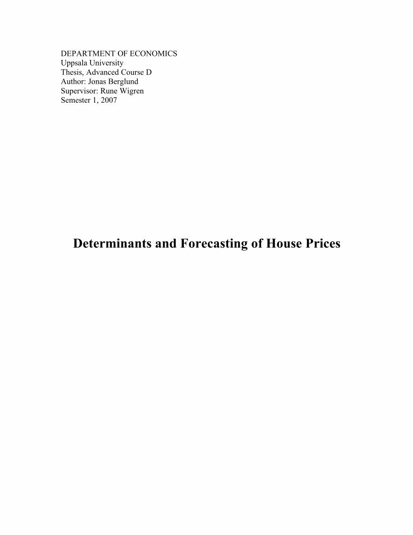
household pays to purchase a house (or apartment). Lastly “construction” is the annual
new construction of housing (in square meters) in the city or area.
Cost of owning (SEK)
(Rent [SEK]) P D Price (SEK) Stock (sq. m.) S Pc Construction (sq. m.) Figure 1: Asset and property markets for real estate The upper right hand quadrant shows the demand for housing depending on the existing
stock of and the annual cost of owning the house6. The demand curve can shift upwards
(downwards) when the number of households that demand housing at the current annual
cost of owning increases (decreases). Since the stock of housing can be assumed to be
fixed in the short run (Anderson, von Essen & Turner, 2004), this quadrant shows how
the annual cost of owning your house is determined from the stock of housing through
the demand-curve.
To acquire the price level of housing in the economy, move to the upper left-hand
quadrant of figure 1. The curve “P” in this section of the model translates the annual cost
of owning a house or an apartment to the price of the house using a capitalization rate (i):
P=CO/i. The capitalization rate is mainly made up by the real-interest rate and an
increase of the interest rate makes the P-curve rotate clockwise around the origin. Higher
6 In the case of a tenant renting his apartment or house from a landlord the cost of owning axis is replaced by the rent specified in the lease.

6
interest will lower the price of a house if the annual cost of owning remains unchanged7.
The capitalization rate is comprised not only by the interest rate but also, for example
influenced by the government tax-code for housing.
In the bottom left-hand quadrant of the model the amount of new housing constructed is
determined. The curve PC represents the cost of replacing real estate and it points down
and left because the cost of new construction is assumed to increase with higher building
activity8 (C). The curve doesn’t go through origin but crosses the price-axis to the left of
the construction-axis because there needs to be some value (the distance origin to where
PC crosses Price-axis) to the new property that is to be constructed. The curve is more
vertical if new real estate construction can be supplied at the same cost, if however there
are impediments in the development of new real estate like for example shortage of land
that make new construction more expensive (inelastic supply of housing) the curve is
more horizontal. The amount of new housing is generated by taking the price-level from
the upper left-hand quadrant down to the cost-of-replacement-curve and then over to the
construction-axis to the right of the quadrant. Lower construction would result in excess
profits due to shortage of supply of housing and higher construction would lead to excess
supply thus being unprofitable to the construction companies. Hence the level of new
construction (C) is determined to be at the level where the price of housing (P) is equal to
cost of replacement (PC).
The remaining quadrant (the bottom right-hand one) is converting the flow of new
construction to the long-run stock of housing. The curve, S, represents the depreciation of
the current stock of housing, i.e. the amount of new housing needed to keep the stock
constant (ΔHousing=0). The more vertical the curve is, the higher is the depreciation rate
and more new construction is needed to keep the stock of housing unchanged. This part
7 In the case of a tenant renting his apartment from a landlord, the capitalization rate is the yield that investors (the landlord) demand to hold real estate assets. It is dependent on the same variables as the case of owner-occupied housing but also for example expected future rents and risk involved in renting. 8 This is amongst other causes because land gets more expensive and higher demand for construction workers makes building more expensive (Wheaton & DiPasquale, 1996).

7
of the model only shows how much new housing is needed to replace the depreciation in
the economy and assumes that the stock of housing is constant over time.
The market is in equilibrium when you complete a full rotation, from the level of stock,
in a counter-clockwise motion back to the level of stock and end up at the same level of
stock as when you started. If you don’t end up at the same level of stock as you started
from, the market is not in equilibrium and cost of owning, price and construction will
have to adjust.
3.1 Positive demand shock
If the demand for housing increases (for example from economic growth or changes in
demographics), the demand-curve shifts up/right, since the stock of housing is fixed the
CO must increase9 which makes the price level increase. Increased price level mean that
more construction projects can be made profitable and therefore the level of construction
increases, which in turn increases the stock of housing in the city concluding the
adjustment to a new market equilibrium (see figure 2).
Cost of owning (SEK)
(Rent [SEK]) P D Price (SEK) Stock (sq. m.) S Pc Construction (sq. m.) Figure 2: The market with increased demand
9 Actually the price increases which means that the CO increases. The reason for this backward impact in the model is that the model’s original form of has rent instead of CO and an increase in demand mean that the landlords can increase the rent from it’s tenants and because of this the price of real estate will increase.

8
3.2 Change in interest rate
If the long-term real interest rate increases, or for example new tax-regulations make it
more expensive to own a house , the P-curve rotates clockwise (see figure 3). The
increased interest rate lowers the price of housing since a household now can spend less
on housing at the same level of CO. The lowered price makes construction of new real
estate less profitable, thus lower construction reduces the stock of housing. This means
that the cost of living has to increase since the same number of people has to share less
housing.
Cost of owning (SEK) (Rent [SEK]) P D Price (SEK) Stock (sq. m.) S Pc
Construction (sq. m.) Figure 3: Increase in long-term interest rates
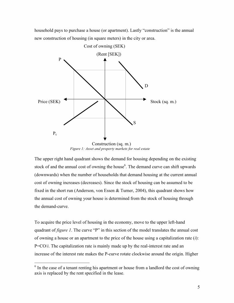
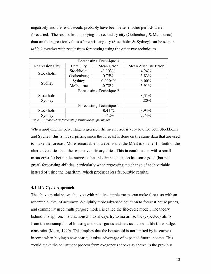
3.3 Change in supply
The supply of new housing can be affected by changes in short-term interest rates or
government regulations (Wheaton & DiPasquale, 1996). If, for example, the short-term
real interest rate falls there will be a positive supply change (see figure 4) increasing
production of new housing which in turn results in an increased stock of hosing.
Increased supply of course leads to lower cost of owning and lower prices on the housing
market. When the housing prices are the same when starting and finishing the lap around
the four squares of the model, equilibrium is reached.
9
Cost of owning (SEK)
(Rent [SEK]) P D Price (SEK) Stock (sq. m.) S Pc
Construction (sq. m.) Figure 4: Positive supply shock 4. VARIABLES The price formation on the housing market seems quite simple when considering the
above theory but what external factors hide behind these neat abbreviations in the theory?
To start with, I assume the depreciation of the housing stock to be fixed; through this the
bottom right quadrant will have no impact on house prices. In the upper left-hand
quadrant, where the interest makes its impact, you can either use real interest or the
nominal. Do households only consider the nominal interest while assessing their financial
situation when buying a house? In an efficient market it is the real interest that should be
used as explanatory variable but since the market is not efficient (Meen, 1999) and
information about the rate of inflation is not as easily accessible as the interest rate, I still
consider it dubious whether to use nominal or real interest. Therefore I will use both at
different times in my analysis.
4.1 A simple model of forecasting
Drake (1993) uses a very simple model where he only includes disposable income,
mortgage interest rate and the number of houses that started construction to set up a
model to forecast UK house prices in the early 1990s. I believe that it would be more

10
accurate to use the number of completed houses instead of number of houses that started
construction. Equation 1 shows my version of Drake’s (1993) forecasting model, from
now on called the “simple model”.
ln P( ) = !
1+ !
2ln Y( ) + !
3R + !
4ln B( ) (1)
Where P= price (or indexed price), Y=disposable income, R=mortgage interest rate and
B= number of new dwellings. One flaw in this estimation is due to the availability (or
lack of it) of data regarding newly constructed dwellings. In the case of Stockholm I use
data for completed housing, however in the case of Sydney no such data is available, I
have used the statistics for building approvals in New South Wales (NSW). This is a
drawback but considering Sydney make up more than half of NSW’s population I assume
it can be used as a good enough proxy. Since an increase in income should increase
demand for housing, the expected sign for the variable “income” is positive. The interest
is according to theory expected to have a negative sign since higher interest increases the
cost of owning which decreases the house prices. Also “new dwellings” are expected to
be negative since increased supply should reduce house prices. The result of the
estimation of the simple model is presented table 1.
Logarithm Percentage change 1989-2006 1989-2004 1989-2006
Variable Sydney Stockholm Sydney Stockholm Sydney Stockholm
Income 2.817 (0.00)
2.190 (0.000)
2.789 (0.000)
2.157 (0.000)
0.924 (0.399)
3.476 (0.000)
Interest 0.002 (0.885)
0.026 (0.146)
0.002 (0.881)
0.028 (0.094)
0.254 (0.717)
-1.688 (0.066)
New dwellings
0.174 (0.512)
0.278 (0.001)
0.212 (0.56)
0.277 (0.000)
0.170 (0.367)
-0.006 (0.971)
Constant -25.516 (0.001)
-14.575 (0.001)
-25.570 (0.002)
-14.182 (0.001)
2.889 (0.705)
4.344 (0.544)
R2 0.935 0.979 0.909 0.981 0.073 0.667 Table 1: Results from regressions using simple forecasting model (p-value in parenthesis)
As seen in table 1, “income” has the expected sign since an increase in income would
increase the house prices according to the theory above. Strangely enough the two other
variables does not have the expected sign in all but one case (the percentage regression

11
for Stockholm). If this model reflects the true conditions, a one percent increase in
disposable income will increase the house prices by 2.8 percent in Sydney and 2.2
percent in Stockholm. This seems to be quite a lot but since the number of regressors in
the model is limited, it is close at hand to think that the variable for income reflects
effects from other variables that have not been included in the model.
The remaining two variables show that if the interest rate increases by one percent, house
prices are virtually unaffected in Sydney and increase by 0.26 percent in Stockholm and
that a similar increase in new housing would increase the average house price by 0.17
percent in Sydney and 0.28 percent in Stockholm. These findings contradict the theory,
however only the only statistically significant variable is the “New dwellings” in
Stockholm. One explanation for the positive sign on “interest” could be that high house
prices are usually a sign of high activity in the economy and interest is increased to cool
down the economy, which could result in high house prices at a high interest rate and
vice versa. In a similar manner the positive sign for “new dwellings” might come from
the high prices on new dwellings. The above theory is for a long run steady state and the
short-run adjustments can differ this state. For example, if lots of new houses are built,
they might increase the price in the short run since new houses are more expensive than
older ones. Another explanation might be that increased prices makes new construction
more profitable and therefore increase construction. In the longer run however the
increased supply might lower the price on the old dwellings – lowering the aggregated
price level. The percentage change regression for Sydney shows a very bad fit (R2 of only
7.3%), however the corresponding regression for Stockholm is the only showing
expected sign for all three explanatory variables and a good fit.
When testing forecasting using the technique of only regressing variables until 2004 and
then forecast the last two years in the dataset (technique 2), the outcome was not very
good for Sydney with a mean error of just less than 5 percent and 8 percent for
Stockholm. In spite of the bad forecasting abilities one must say that it is the latter years
of the time series that show the largest differences between the calculated result and the
real outcome. It is likely that this affects the second techniques forecasting abilities
12
negatively and the result would probably have been better if other periods were
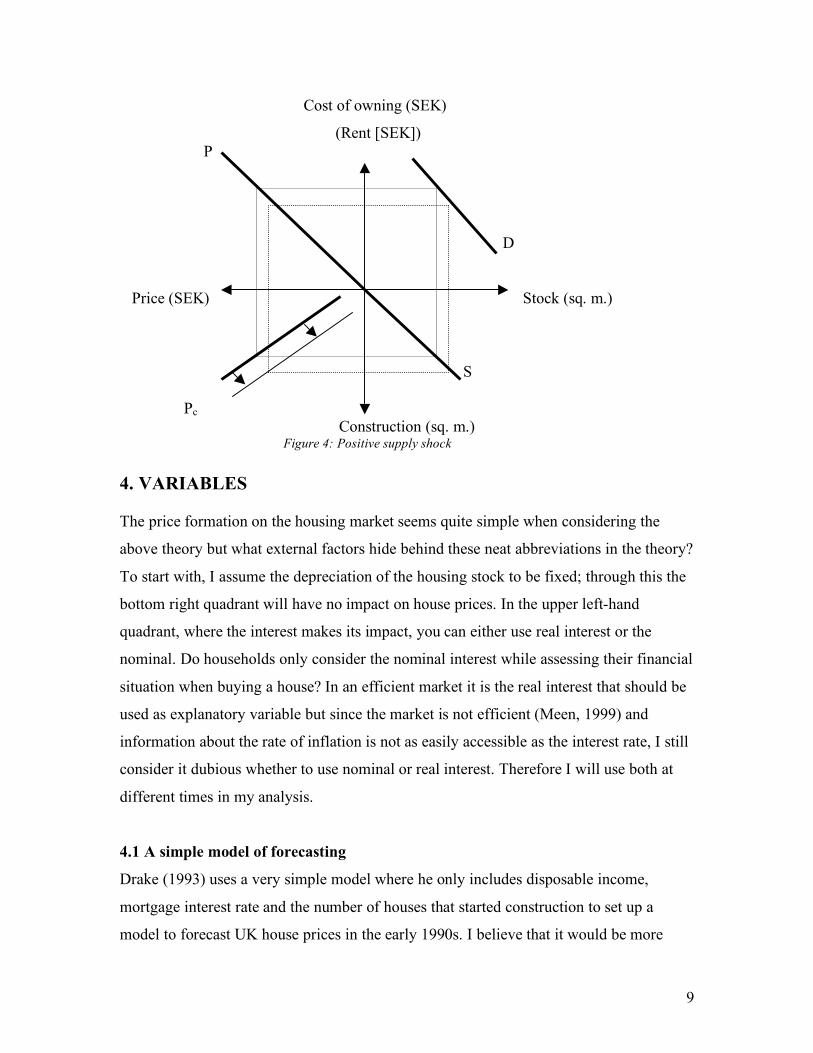
forecasted. The results from applying the secondary city (Gothenburg & Melbourne)
data on the regression values of the primary city (Stockholm & Sydney) can be seen in
table 2 together with result from forecasting using the other two techniques.
Forecasting Technique 3
Regression City Data City Mean Error Mean Absolute Error Stockholm -0.003% 4.24% Stockholm Gothenburg 0.75% 3.83%
Sydney -0.0004% 6.00% Sydney Melbourne 0.70% 5.91% Forecasting Technique 2
Stockholm 8,51% Sydney 4.80%
Forecasting Technique 1 Stockholm -0,41 % 3.94%
Sydney -0.42% 7.74% Table 2: Errors when forecasting using the simple model When applying the percentage regression the mean error is very low for both Stockholm
and Sydney, this is not surprising since the forecast is done on the same data that are used
to make the forecast. More remarkable however is that the MAE is smaller for both of the
alternative cities than the respective primary cities. This in combination with a small
mean error for both cities suggests that this simple equation has some good (but not
great) forecasting abilities, particularly when regressing the change of each variable
instead of using the logarithm (which produces less favourable results).
4.2 Life Cycle Approach
The above model shows that you with relative simple means can make forecasts with an
acceptable level of accuracy. A slightly more advanced equation to forecast house prices,
and commonly used multi purpose model, is called the life-cycle model. The theory
behind this approach is that households always try to maximize the (expected) utility
from the consumption of housing and other goods and services under a life time budget
constraint (Meen, 1999). This implies that the household is not limited by its current
income when buying a new house; it takes advantage of expected future income. This
would make the adjustment process from exogenous shocks as shown in the previous
13
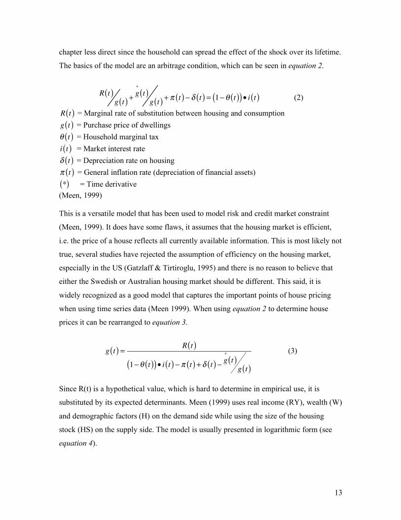
chapter less direct since the household can spread the effect of the shock over its lifetime.
The basics of the model are an arbitrage condition, which can be seen in equation 2.
R t( )g t( )
+g*
t( )g t( )
+ ! t( ) " # t( ) = 1"$ t( )( ) • i t( ) (2)
R t( ) = Marginal rate of substitution between housing and consumption g t( ) = Purchase price of dwellings ! t( ) = Household marginal tax i t( ) = Market interest rate ! t( ) = Depreciation rate on housing ! t( ) = General inflation rate (depreciation of financial assets) *( ) = Time derivative
(Meen, 1999) This is a versatile model that has been used to model risk and credit market constraint
(Meen, 1999). It does have some flaws, it assumes that the housing market is efficient,
i.e. the price of a house reflects all currently available information. This is most likely not
true, several studies have rejected the assumption of efficiency on the housing market,
especially in the US (Gatzlaff & Tirtiroglu, 1995) and there is no reason to believe that
either the Swedish or Australian housing market should be different. This said, it is
widely recognized as a good model that captures the important points of house pricing
when using time series data (Meen 1999). When using equation 2 to determine house
prices it can be rearranged to equation 3.
g t( ) =R t( )
1!" t( )( ) • i t( ) ! # t( ) + $ t( ) !g*
t( )g t( )
(3)
Since R(t) is a hypothetical value, which is hard to determine in empirical use, it is
substituted by its expected determinants. Meen (1999) uses real income (RY), wealth (W)
and demographic factors (H) on the demand side while using the size of the housing
stock (HS) on the supply side. The model is usually presented in logarithmic form (see
equation 4).

14
ln(g) = f (ln RY( ), ln W( ), ln H( ), ln HS( ), ln 1!"( )i + # ! $ ! g*
g
%
&''
(
)**
(4)
A problem with this equation is the last term, which represents real interest. It can under
some circumstances be a negative number, which cannot be logarithmic. Usually the
method to deal with this is to express a semi logarithmic relationship between real house
prices and interest rate. In the data for this survey the real interest is not negative for any
of the countries that makes it possible to use it in the survey. The regression with which I
will test this method of forecasting is given by equation 5, from now on called the “life
cycle model”.
ln(P) = !1 + !2 ln(RY ) + !3H + !4 ln W( ) + !´5 ln(HS) + !6RI (5)
As the demographic factor (H) I use, in accordance with Brown, Song & McGillivray
(1997), the percentage of population under 26 years of age. This is because this age group
is less likely to move than the other which in the above theory will shift the demand
curve down/left and ultimately lead to a decrease in house prices if the part of under 26”s
increases. The factor (RY) will affect the demand curve in an opposite fashion if the
income of the population increases. An increase in the factor HS (Stock of housing) will
cause the house prices to fall by shifting the PC-curve down/left. As shown, equation 5
gets input from all quadrants of the theoretical model and should therefore be more
accurate in explaining house prices than the simple model. The results from estimating
the life cycle model are shown in table 3.

15
Kind of
regression Logarithm regression Percentage change
1989-2006 1989-2004 1989-2006 Variable Sydney Stockholm Sydney Stockholm Sydney Stockholm
Income 0.899 (0.604)
8.874 (0.014)
1.367 (0.385)
8.357 (0.022)
-0.506 (0.413)
3.586 (0.036)
Part of Under 26”s
0.479 (0.087)
0.676 (0.116)
0.736 (0.019)
0.465 (0.314)
-1.134 (0.459)
-1.405 (0.922)
Wealth 1.075 (0.094)
-0.451 (0.257)
2.352 (0.019)
-0.562 (0.182)
-1.528 (0.005)
-0.007 (0.981)
Stock of Housing
9.220 (0.035)
-22.264 (0.082)
8.183 (0.038)
-21.063 (0.101)
-1.508 (0.371)
4.051 (0.704)
Interest -0.018 (0.655)
-0.006 (0.882)
-0.024 (0.500)
-0.004 (0.923)
-2.362 (0.072)
-1.269 (0.557)
Constant -161.285 (0.023)
166.777 (0.122)
-174.736 (0.009)
165.95 (0.126)
81.94 (0.110)
41.719 (0.921)
R2 0.962 0.960 0.966 0.957 0.763 0.631 Table 3: Results from regression using the life cycle model (p-value in parenthesis) In table 3 the variables for “income” and “interest” show expected sign for most of the
regressions even though only the “income”-variable in Stockholm are statistically
significant. The demographic variable only showing expected sign in the percentage
regressions and yet again generally not significant results. The sign of the other two
regressors vary between the cities. The interpretation of the logarithmic equations is that
if the average income in Sydney increases by one percent, the average house price will
increase by 0.899 percent. This sounds reasonable in contrast to the corresponding value
for Stockholm that predicts house prices to increase by 8.874 percent from a one percent
increase in disposable income. This number seems a bit too high but it is hard to
determine why the model shows these results. The Demographics variable is consistent
and fairly similar in both the logarithmic regressions where it should be interpreted as a
one percent increase of the ratio of under 26’s to the population as a whole, the house
prices increase by 0.47 and 0.73 percent.
As with “income”, the variable “wealth” looks good for Sydney but not for Stockholm, it
is hard to believe that an increase in wealth would cause a decrease in housing prices. If
the general wealth of the population would increase it should cause an increase in
16
demand, which according to the above theory increase the house prices. The supply-
variable also shows some strange characteristics in this model. According to the theory a
bigger stock of housing should decrease the price of housing, this is the case in the
Stockholm regression but the value seems a bit high, I find it hard to believe that a one
percent increase in the stock of housing would lower the average house price by more
than a fifth. In opposite fashion the value of the average Sydney house would increase in
value by almost 10 percent when the stock of housing increases by one percent. Lastly
the variable for interest is consistent with the theory since the model predicts a price fall,
although very marginal, when the interest increases. In short the model seems to have
some inconsistencies when you compare it to the theory.
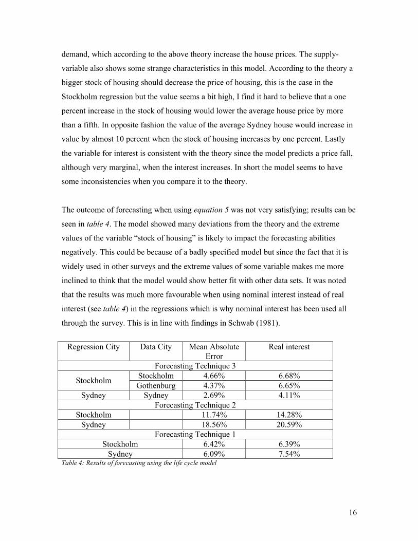
The outcome of forecasting when using equation 5 was not very satisfying; results can be
seen in table 4. The model showed many deviations from the theory and the extreme
values of the variable “stock of housing” is likely to impact the forecasting abilities
negatively. This could be because of a badly specified model but since the fact that it is
widely used in other surveys and the extreme values of some variable makes me more
inclined to think that the model would show better fit with other data sets. It was noted
that the results was much more favourable when using nominal interest instead of real
interest (see table 4) in the regressions which is why nominal interest has been used all
through the survey. This is in line with findings in Schwab (1981).
Regression City Data City Mean Absolute
Error Real interest
Forecasting Technique 3 Stockholm 4.66% 6.68% Stockholm Gothenburg 4.37% 6.65%
Sydney Sydney 2.69% 4.11% Forecasting Technique 2
Stockholm 11.74% 14.28% Sydney 18.56% 20.59%
Forecasting Technique 1 Stockholm 6.42% 6.39%
Sydney 6.09% 7.54% Table 4: Results of forecasting using the life cycle model
17
Since data for the stock of housing in Melbourne does not exist, the city has not been
used in this section. The errors in the logarithmic forecasts are at the same level as for the
previous equation. As in forecasting using the simple model, the MAE is smaller for the
alternative city; this is an indication that the model has good forecasting abilities, at least
for Stockholm. The main problem is still that the predictions are not accurate enough. An
Absolute Error of more than four percent is not very good. Reasons for this might be bad
dataset or a poorly specified model.
5. IMPLEMENTATION OF AN ARMA-MODEL One problem of the above models is that the housing markets do not react instantly to the
change in the explaining variables. Big changes in exogenous variables will get too much
of an impact when using simple OLS regression. To counter the problem of inaccurate
predictions one way is to use an autoregressive moving average (ARMA) model. This
introduces two new elements to the modelling. The first being an autoregressive element,
this means that it not only uses the explanatory variable as input but also past values of
the dependent variable. In short the present change in price is being determined by the
explanatory variables and house price changes in the past. The second new element is the
usage of moving average of the variables; hence a one-off deviation in one of the
variables will not affect the outcome as much as before. These improvements should have
a positive impact since the earlier estimations show low mean average but a rather high
absolute mean average.
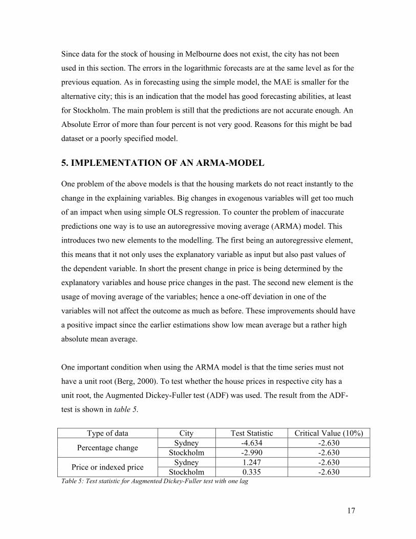
One important condition when using the ARMA model is that the time series must not
have a unit root (Berg, 2000). To test whether the house prices in respective city has a
unit root, the Augmented Dickey-Fuller test (ADF) was used. The result from the ADF-
test is shown in table 5.
Type of data City Test Statistic Critical Value (10%)
Sydney -4.634 -2.630 Percentage change Stockholm -2.990 -2.630 Sydney 1.247 -2.630 Price or indexed price Stockholm 0.335 -2.630
Table 5: Test statistic for Augmented Dickey-Fuller test with one lag
18
As seen in table 5, the hypothesis of unit root could be rejected on the 10 percent level
for both cities when using the percentage change, which makes it possible to use ARMA.
The result also indicates that I cannot use the logarithmic estimations since the null
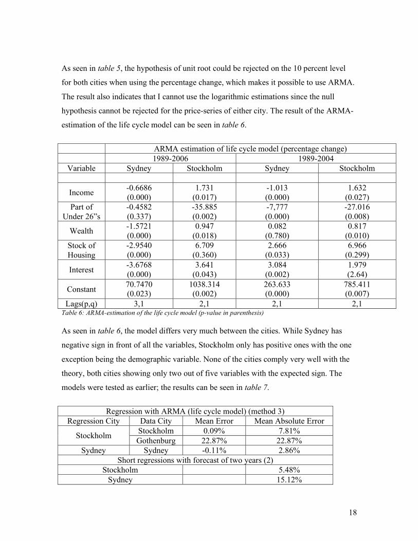
hypothesis cannot be rejected for the price-series of either city. The result of the ARMA-
estimation of the life cycle model can be seen in table 6.
ARMA estimation of life cycle model (percentage change) 1989-2006 1989-2004
Variable Sydney Stockholm Sydney Stockholm
Income -0.6686 (0.000)
1.731 (0.017)
-1.013 (0.000)
1.632 (0.027)
Part of Under 26”s
-0.4582 (0.337)
-35.885 (0.002)
-7,777 (0.000)
-27.016 (0.008)
Wealth -1.5721 (0.000)
0.947 (0.018)
0.082 (0.780)
0.817 (0.010)
Stock of Housing
-2.9540 (0.000)
6.709 (0.360)
2.666 (0.033)
6.966 (0.299)
Interest -3.6768 (0.000)
3.641 (0.043)
3.084 (0.002)
1.979 (2.64)
Constant 70.7470 (0.023)
1038.314 (0.002)
263.633 (0.000)
785.411 (0.007)
Lags(p,q) 3,1 2,1 2,1 2,1 Table 6: ARMA-estimation of the life cycle model (p-value in parenthesis) As seen in table 6, the model differs very much between the cities. While Sydney has
negative sign in front of all the variables, Stockholm only has positive ones with the one
exception being the demographic variable. None of the cities comply very well with the
theory, both cities showing only two out of five variables with the expected sign. The
models were tested as earlier; the results can be seen in table 7.
Regression with ARMA (life cycle model) (method 3)
Regression City Data City Mean Error Mean Absolute Error Stockholm 0.09% 7.81% Stockholm Gothenburg 22.87% 22.87%
Sydney Sydney -0.11% 2.86% Short regressions with forecast of two years (2)
Stockholm 5.48% Sydney 15.12%
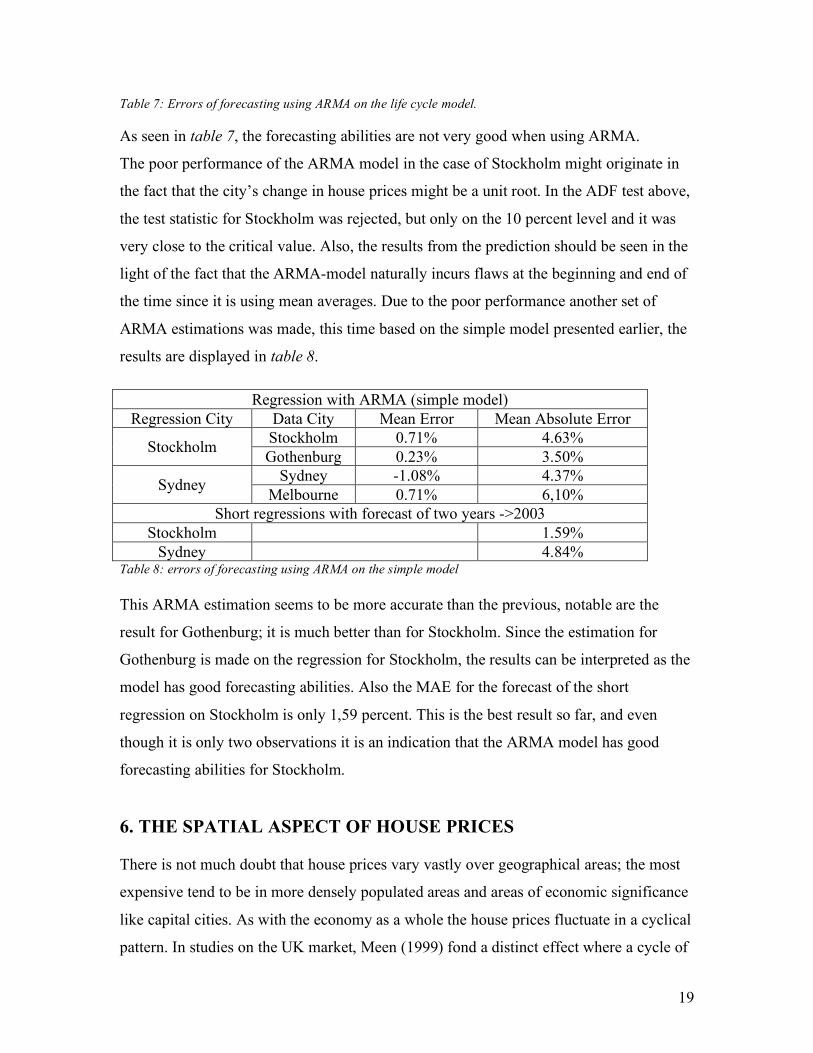
19
Table 7: Errors of forecasting using ARMA on the life cycle model. As seen in table 7, the forecasting abilities are not very good when using ARMA.
The poor performance of the ARMA model in the case of Stockholm might originate in
the fact that the city’s change in house prices might be a unit root. In the ADF test above,
the test statistic for Stockholm was rejected, but only on the 10 percent level and it was
very close to the critical value. Also, the results from the prediction should be seen in the
light of the fact that the ARMA-model naturally incurs flaws at the beginning and end of
the time since it is using mean averages. Due to the poor performance another set of
ARMA estimations was made, this time based on the simple model presented earlier, the
results are displayed in table 8.
Regression with ARMA (simple model) Regression City Data City Mean Error Mean Absolute Error
Stockholm 0.71% 4.63% Stockholm Gothenburg 0.23% 3.50% Sydney -1.08% 4.37% Sydney Melbourne 0.71% 6,10%
Short regressions with forecast of two years ->2003 Stockholm 1.59%
Sydney 4.84% Table 8: errors of forecasting using ARMA on the simple model This ARMA estimation seems to be more accurate than the previous, notable are the
result for Gothenburg; it is much better than for Stockholm. Since the estimation for
Gothenburg is made on the regression for Stockholm, the results can be interpreted as the
model has good forecasting abilities. Also the MAE for the forecast of the short
regression on Stockholm is only 1,59 percent. This is the best result so far, and even
though it is only two observations it is an indication that the ARMA model has good
forecasting abilities for Stockholm.
6. THE SPATIAL ASPECT OF HOUSE PRICES There is not much doubt that house prices vary vastly over geographical areas; the most
expensive tend to be in more densely populated areas and areas of economic significance
like capital cities. As with the economy as a whole the house prices fluctuate in a cyclical
pattern. In studies on the UK market, Meen (1999) fond a distinct effect where a cycle of

20
house prices originated in the South-East of England, more specifically London, to then
spread through the rest of the country over time. This is called the “ripple effect” and it
has been used by for example Giussani & Hadjimateou (1991) and Munro & Tu (1996) to
use house price changes in London as an exogenous variable when explaining the
movements of house prices in other parts of Britain. You could interpret this in the way
that the house price cycle starts in England’s Economic centre, London, and then spreads
like a wave in the ocean over Britain. It seems plausible that the ripple effect occurs in
any market. In the very complicated set of relationships that make up a country’s
economy it seems likely that the house prices are firstly affected where the most
economic activity occurs and then ripple out over the country. But is this effect limited to
single economic markets or could you apply the ripple effect to an international level?
Translating the ripple effect of the UK to a national level would mean that the house
prices of Stockholm or Sydney could be influenced by global economic centres such as
the EU, US or economically more powerful countries like England. To quickly examine
this, the percentage change of house prices in Stockholm and Sydney as well as other
economically strong countries (UK (Nationwide, 2007) and USA (OPHEO, 2007)) are
plotted in a graph in figure 5.
Figure 5: Percentage change of house prices in different regions

21
From figure 5 one can see that there seems to be low correlation between the
development of Stockholm’s house prices and the development of aggregated house
prices in the UK and the US. Even so, there seems to be correlation between Stockholm
and the house prices in London. The coefficient of correlation between the two is 0.77.
During almost the entire eighties the change in house prices in London and Stockholm
are almost identical. When studying the few entries from 2000 onwards the price changes
differs slightly but it still seems reasonable to use the change in London house prices as a
regressor for house price change in Stockholm. The problem here is the causality, is it
London that leads and Stockholm that follows or vice versa or is it just a coincidence?
You cannot say from this simple graph but I find it more believable that Stockholm
follows London since the literature on the ripple effect specifies economic centres as the
origin (MacDonald & Taylor, 1993) and smaller cities as followers and there should be
no doubt that London is a bigger player on the stage of world economics than Stockholm.
From the graph one could suspect that the house prices for the UK could be used as an
explanatory variable for the Sydney house prices (Coefficient of correlation = 0.75). The
geographical distance however makes it a bit far fetched to use this causality in a
forecasting model. Due to difficulty in obtaining reliable data from Asia-pacific nations,
the Sydney house prices will not be covered in this part of the survey.
To test whether there is any use to utilize the London house prices as an indicator on
what will happened in Stockholm, a series of regressions was estimated. The difference
to the new estimations being that the house prices in London were added as an
explanatory variable. The result from the forecast using these new estimations can be
seen in tables 9 and 10. Notable here is that the estimations yield a lower MAE when
using London prices as an exogenous variable in all but one case. Also note that the
simple model with fewer explanatory variables outperforms the life cycle model on
several occasions, both with and without the extra variable of London house prices. This
might be because the life cycle method catches the same effect in two of the explanatory
variables giving the effect too much of an impact. For example, both “wealth” and
“income” cover an increase in demand when households increases (or decreases) its
economic strength.

22
Life Cycle model (Stockholm) Regression Mean Absolute Error
Excluding London Including London Logarithm Full (1) OLS 6.42% 1.46% Logarithm short (2) OLS 11.74% 3.98%
ARMA 7.81% 2.83% Percentage (3) OLS 4.66% 2.90% ARMA 5.63% 10.56% Gothenburg
(On Stockholm estimation) OLS 4.37% 9.45%
Table 9: MAE for forecasting Stockholm house prices using the life cycle model
Simple model (Stockholm) Regression Mean Absolute Error
Excluding London Including London Logarithm Full (1) OLS 3.94% 1.70% Logarithm short (2) OLS 1.49% 2.77%
ARMA 4.63% 2.79% Percentage (3) OLS 4.24% 2.78% ARMA 3.47% 4,34% Gothenburg
(On Stockholm estimation) OLS 3.83% 4.28%
Table 10: MAE for forecasting Stockholm house prices using the simple model
The inclusion of the London house prices to the models seems to be beneficial to the
forecasting abilities. The MAE is lower for most of the forecasts, the only exceptions
being when the Stockholm estimation is applied to data for Gothenburg and when using
estimation technique 2 for the simple model but the latter is only increased slightly from
an exceptionally good result. The bad forecasting for the alternate city (Gothenburg)
could be because Gothenburg is to small to be affected by the house price change in
London or that it takes longer for the effect of London housing prices to ripple to
Gothenburg that it is not covered by these models. If the latter were the case the
estimations would probably be better if you a one-year lag was used for the London
house prices when estimating the forecasting model for Gothenburg.
7. FINANCIAL INDICATORS To many households, the house they live in is their biggest financial asset (Tsatsaronis &
Zhu, 2004). This makes housing an interesting mix of investment and consumption; the
household consumes housing services while at the same time making an investment in

23
the house. Looking at house prices from an investment point of view one might suspect
that you could be able to use other alternatives of investment as an indicator of house
price movements. The stock market is an easy option for an investigation of the financial
markets implication on house prices. Earlier literature is indecisive on its implications on
house prices. Chen and Patel (1998) finds that the stock market has a positive effect on
house prices in Taipei and Sutton (2002) show similar results for 6 industrialized
countries whilst for example Wilson, Okunev and Ta (1996) find it inconclusive to
whether the Real Estate and securities, such as the stock market, affect each other. If in
fact the two markets are integrated the question remains wether the markets are
substitutes or complements. The correlation test between the change in Sydney house
prices and the change in the ASX/200 (RBA, 2007b) of the Australian Stock Exchange
show a correlation of -0.503. In figure 6 the change in stock index has been inverted for
viewing purposes. Also included in figure 6 are two other financial indicators that were
chosen from a number of financial indicators due to high correlation with the change in
house prices10.
Figure 6: Percentage change in Sydney house prices and a number of financial indicators
10 These indicators are the household debt-to-asset (D-t-A) and debt-to-disposable income (D-t-I) ratios (RBA, 2007c)

24
Despite a relatively low correlation, the house price and stock index show a very similar
pattern during the latter ten years of the time period. The reason for the difference in the
early 1990’s is unknown. The sign of negative correlation between the stock market and
house prices are likely to come from the fact the that Real Estate is considered a safer
investment than stocks. When the stock market is crumbling and uncertainty about the
future rises, investors might turn to real estate to protect their assets thus increasing the
demand for housing which according to the theory will increase house prices. Another
financial indicator that seems to help pointing out in which direction house prices are
going is the debt-to-income (D-t-I) ratio, with a coefficient of correlation of 0.68, and as
seen in figure 6, this should be a good explanatory variable of house price changes. The
causality should be fairly straightforward: if the ratio is high the households has greater
difficulty in raising money to buy new houses, thus decreasing the demand which
according to the theory affects the house prices negatively. Unfortunately data covering
the debt-to-income ratio is not available for the Swedish market, which is why only
Sydney will be examined in this part of the survey.
Simple model (Sydney) Debt-to-Income Ratio
Regression Mean Absolute Error Original model Including D-t-I Ratio Including
Stock Market Logarithm Full (1) OLS 7.74% 5.29% 7.89%
Logarithm Short (2) OLS 4,58% 5.77% 5,52% ARMA 6.48% 4.58% 4.55% Percentage (3) OLS 4.24% 4.44% 3.79% ARMA 6.54% 5.52% 4.53% Melbourne
(On Sydney estimation) OLS 5.91% 5.48% 3.56%
Table 11: Errors when forecasting using financial indicators in the simple model
Life-Cycle Model (Sydney) Stock Market Regression Mean Absolute Error
Original model Including D-t-I Ratio Including Stock Market
Logarithm Full (1) OLS 6.09% 4.56% 3.04% Logarithm Short (2) OLS 12.86% 7.54% 7.43%
ARMA 2.86% 2.36% 2.37% Percentage (3) OLS 4.37% 2.29% 2.30% Table 12: Errors when forecasting using financial indicators in the life cycle model

25
There is no doubt both the debt-to-income ratio and the performance of the stock market
has a positive effect on the forecasting abilities of both the models. In the life cycle
model it almost makes no difference which of the two new explaining variables to use,
they only differ significantly on one of the methods of estimation. In the simple model it
seems like the change in stock market has more of a positive effect than using the debt-
to-income ratio, performing better on all but one of the estimations. An explanation to the
better performance when using the stock market as exogenous variable is that it has a
more direct and visible effect on households than the D-t-I ratio. When the stock market
is performing badly some investors might go straight to the real estate market while the
D-t-I ratio mainly affects households which might be slower in it’s adjustments to a
higher D-t-I. Another reason might be that banks lend money easier in times of good
economic outlook; increasing the D-t-I ratio to higher levels than it would when house
price increases are moderate or falling. This would result in a situation with both
increasing house prices and increasing D-t-I ratio, which is opposite to the initial idea of
the effect on house prices.
8. CONCLUDING REMARKS The main determinants of house prices seem to be nominal interest, household income
and the supply of new dwellings. These are explanatory variables in one of the models
presented in this paper. Also presented was a more complicated model with more
exogenous variables, however this “life cycle” model failed to create a better overall
forecast despite including more explanatory variables. The simple model outperformed
its more advanced counterpart on all forecasting of the Stockholm house prices. On the
Sydney market the outcome was more favourable for the life cycle model but the simple
model was close behind with acceptable AME’s. The addition of financial indicators to
the regressions has some positive effects in this survey. Which indicator to use however
cannot be determined, the two investigated indicators seem booth to have pros and cons.
The choice of proffered indicator also seems to depend on which model is being used.
The most interesting finding is however that the so called “ripple effect” seems to be
applicable to an international level since the errors of forecasting was consistently lower

26
by a considerable margin when including the London house prices as an explanatory
variable for the Stockholm house prices. To determine the existence of this effect further
research is needed to establish the causality of this international ripple effect.

27
9. REFERENCES ABS, (2007a), ”House Price Indexes: Eight Capital Cities, Table 10. Established Hose Price Index”, Available [Online]: http://www.abs.gov.au/ausstats/[email protected]/log?openagent&641603.xls&6416.0&Time%20Series%20Spreadsheet&017D4699E10A5CB7CA2572D50028C580&0&Mar%202007&09.05.2007&Latest. [2007-05-10]. ABS, (2007b), “Household Income and Income Distribution, Australia”, Available [Online]: http://www.abs.gov.au/ausstats/subscriber.nsf/log?openagent&6523055001_2003_04.xls&6523.0.55.001&Data%20Cubes&CA2568A90021A807CA256F41007C8505&0&2003-04&04.08.2005&Latest [2007-05-10]. ABS, (2007c), “CPI: All Groups, Index Numbers and Percentage Changes, Tables 1 & 2, Available: [Online]: http://www.abs.gov.au/AUSSTATS/[email protected]/log?openagent&640101.zip&6401.0&Time%20Series%20Spreadsheet&CB6BE7EA5027821CCA2572C6001D698A&0&Mar%202007&24.04.2007&Latest. [2007-05-10]. ABS, (2007d), “Australian National Accounts: Financial Accounts, Table 15”, Available [Online]: http://www.abs.gov.au/AUSSTATS/[email protected]/log?openagent&5232015.xls&5232.0&Time%20Series%20Spreadsheet&47D18B10B6E7123ACA2572AD0021E044&0&Dec%202006&30.03.2007&Latest. [2007-05-10]. ABS, (2007e), “Population Change – Australia. Table 1”, Available: [Online]: http://www.abs.gov.au/ausstats/[email protected]/log?openagent&310101.xls&3101.0&Time%20Series%20Spreadsheet&39B992B00C6C0992CA2572A500188FD7&0&Sep%202006&22.03.2007&Latest. [2007-05-10]. ABS, (2007f), “Housing Choices, NSW” Available: [Online]: http://www.abs.gov.au/ausstats/subscriber.nsf/log?openagent&32401_oct%202004.pdf&3240.1&Publication&CB5881C52C8A0FDECA256FD500772A61&0&Oct%202004&01.04.2005&Latest [2007-05-10]. ABS, (2007g), “Census of Population and Housing: Selected Characteristics for Urban Centres and Localities, New South Wales and Australian Capital Territory, 2001” Available: [Online]: http://www.abs.gov.au/ausstats/subscriber.nsf/log?openagent&20161_2001.pdf&2016.1&Publication&886D29420372B32CCA256CF40001EA95&0&2001&25.03.2003&Latest. [2007-05-10].

28
ABS, (2007h), “Building Approvals, Australia. Table 22”, Available: [Online]: http://www.abs.gov.au/ausstats/[email protected]/log?openagent&87310022.xls&8731.0&Time%20Series%20Spreadsheet&88AE15C50A6598DDCA2572D4001C1A59&0&Mar%202007&08.05.2007&Latest. [2007-05-10]. Barot, B. & Yang, Z., (2002), “House Prices and Housing Investment in Sweden and the United Kingdom. Econometric Analysis for the Period 1970-1998” Review of Urban Development Studies, Vol. 14, No. 2. Berg, L., (2000), “Småhuspriser på Andrahandsmarknaden – Samvariation, Påverkan och Bestämningsfaktorer” I Lindh, T., “Prisbildning och Värdering av Fastigheter”, Gävle Brown, J. P., Song, H. & McGillivray, A., (1997), “Forecasting UK House Prices: A Time Varying Coefficient Approach”, Economic Modelling, Vol. 14, pp. 529-548. Chen, M-C. & Patel, K., (1998), “House Price Dynamics and Granger Causality: An Analysis of Taipei New Dwelling Market”, Journal of Asian Real Estate Society, Vol. 1, No. 1, pp. 101-126. DiPasquale, D. & Wheaton, W. C. (1996), Urban Economics and Real Estate Markets. New Jersey. Drake, L., (1993), “Modelling UK House Prices Using Cointegration: An Application of the Johansen Technique”, Applied Economics, Vol. 25, pp 1225-1228. Gatzlaff, D. & Tirtiroglu, D. (1995) ”Real Estate Market Efficiency: Issues and Evidence” Journal of Real Estate Literature, Vol. 3, No. 2, pp 157-192 Giussani & Hadjimateou (199) “Modelling regional House Prices In the United Kingdom.” Papers in Regional Science, Vol. 70, No. 2. Hort, K., (1998), “The Determinants of Urban House Price Fluctuations in Sweden” 1968-1994”, Journal of Housing Economics, Vol. 7, No. 2, pp. 93-120. Jud, G. D. & Winkler, D. T., (2002), “The Dynamics of Metropolitan housing Prices”, Journal of Real Estate Research, Vol. 23, No. 1. MacDonald, R. & Taylor, M., P., (1993), “Regional House Prices In Britain: Long-Run Relationships and Short Run Dynamics”, Scottish Journal of Political Economy, Vol. 40, No. 1, pp. 43-55. Meen, G., (1999), “Regional house Prices and the Ripple Effect: A New Interpretation”, Housing Studies, Vol. 14, No. 6, p.p. 733-753. Munro, M. & Tu, Y. (1996) “UK House Price Dynamics: Past and Future Trends – a Technical Paper”. CML Discussion Papers. London
29
Nationwide, (2007) “UK House Prices Since 1952” Available [Online]: http://www.nationwide.co.uk/hpi/historical.htm [2007-05-10]. “New South Wales In Focus” (2006), Available [Online]: http://www.abs.gov.au/ausstats/subscriber.nsf/log?openagent&13381_2006.pdf&1338.1&Publication&56136D2A6373AE90CA25719B000756C3&0&2006&28.06.2006&Latest. [2007-05-10]. OPHEO (2007), “U.S. House Price Appreciation Rate Steadies”, Available [Online]: http://www.ofheo.gov/media/pdf/4q06hpi.pdf [2007-05-10]. RBA, (2007a), “Indicator Lending Rates – F5”, Available [Online]: http://www.rba.gov.au/Statistics/Bulletin/F05hist.xls. [2007-05-10]. RBA, (2007b), “F07 Share Market” Available: [Online]: http://www.rba.gov.au/Statistics/Bulletin/F07hist.xls. [2007-05-10]. RBA (2007c), “B21 Household Finances – Selected Ratios” Available: [Online]: http://www.rba.gov.au/Statistics/Bulletin/B21hist.xls [2007-05-10]. Riksbanken, (2007), ”Mortgage Bonds”, Available [Online]: http://www.riksbank.com/templates/stat.aspx?id=17191. [2007-05-10]. SCB, (2007a), ”Försålda småhus efter län. År”, Available: [Online]: http://www.ssd.scb.se/databaser/makro/visavar.asp?yp=duwird&xu=c5587001&lang=1&langdb=1&Fromwhere=S&omradekod=BO&huvudtabell=FastprisSHRegionAr&innehall=Antal&prodid=BO0501&deltabell=L1&fromSok=&preskat=O. [2007-05-10]. SCB, (2007b), “Sammanräknad förvärvsinkomst för boende I Sverige den 31/12 respektive år efter län, kön, ålder och inkomstklass. År”, Available: [Online]: http://www.ssd.scb.se/databaser/makro/visavar.asp?yp=duwird&xu=c5587001&lang=1&langdb=1&Fromwhere=S&omradekod=HE&huvudtabell=SamForvInk2&innehall=SamForvInkMedel&prodid=HE0108&deltabell=L1&fromSok=&preskat=O. [2007-05-10]. SCB, (2007c), “CPI, Fixed Numbers”, Available: [Online]: http://www.scb.se/templates/tableOrChart____33848.asp. [2007-05-10]. SCB, (2007d), “Hushållens Ställning och Transaktion” Available [Online]: http://www.scb.se/statistik/FM/FM0105/2007K01/Sparbarometern%202007k1.xls [2007-05-10]. SCB, (2007e), “Befolkningen Efter Län, Civilstånd, Ålder och Kön. År” Available: [Online]: http://www.ssd.scb.se/databaser/makro/visavar.asp?yp=duwird&xu=c5587001&lang=1&langdb=1&Fromwhere=S&omradekod=BE&huvudtabell=Befolkning&innehall=Folkmangd&prodid=BE0101&deltabell=L&fromSok=&preskat=O. [2007-05-10].

30
SCB, (2007f), “Kalkylerat Bostadsbestånd Efter Län och Hustyp. År” Available: [Online]: http://www.ssd.scb.se/databaser/makro/visavar.asp?yp=duwird&xu=c5587001&lang=1&langdb=1&Fromwhere=S&omradekod=BO&huvudtabell=BostadsbestandK&innehall=Bostadsbestand&prodid=BO0104&deltabell=L1&fromSok=&preskat=O. [2007-05-10]. SCB, (2007g), “Färdigställda Lägenheter och Rumsenheter i Nybyggda Hus Efter Län och Hustyp. År”, Available: [Online]: http://www.ssd.scb.se/databaser/makro/visavar.asp?yp=duwird&xu=c5587001&lang=1&langdb=1&Fromwhere=S&omradekod=BO&huvudtabell=LghReHustypAr&innehall=AntLgh&prodid=BO0101&deltabell=L1&fromSok=&preskat=O. [2007-05-10]. Schwab, R. M., (1983), “Real and Nominal Interest Rates and the Demand for Housing”, Journal of Urban Economics, Vol. 13, pp. 181-195. Sutton, G., (2002), “Explaining Changes in Housing Prices”, BIS Quarterly Review, September, pp. 46-55 Tsatsaronis, K. & Zhu, H.,, (2004), “What Drives House Price Dynamics: Cross-Country Evidence” BIS Quarterly Review, March 2004 Wilson, P., Okunev, J. & Ta, G., (1996), “Are Real Estate and Securities Markets Integrated? Some Australian Evidence”, Journal of Property Valuation & Investment, Vol. 14, No. 5, pp. 7-24. “Yearbook Australia 2006” (2006), Available [Online]: http://www.abs.gov.au/ausstats/subscriber.nsf/log?openagent&13010_2006.pdf&1301.0&Publication&67E47661AA446A24CA2570FC00119006&0&2006&20.01.2006&Previous. [2007-05-10].